.1

Transportation and Assignment Problems

.2

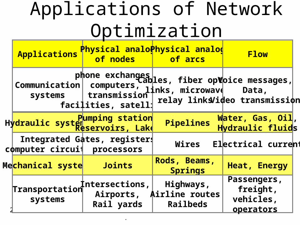
ApplicationsPhysical analog

of nodes Physical analog

of arcsFlow

Communicationsystems

phone exchanges, computers, transmission

facilities, satellites

Cables, fiber optic links, microwave

relay links

Voice messages, Data,

Video transmissions

Hydraulic systemsPumping stationsReservoirs, Lakes

PipelinesWater, Gas, Oil,Hydraulic fluids

Integrated computer circuits

Gates, registers,processors

Wires Electrical current

Mechanical systems JointsRods, Beams,

SpringsHeat, Energy

Transportationsystems

Intersections, Airports,

Rail yards

Highways,Airline routes

Railbeds

Passengers, freight,

vehicles, operators

Applications of Network Optimization

.3

Description

A transportation problem basically deals with the problem, which aims to find the best way to fulfill the demand of n demand points using the capacities of m supply points. While trying to find the best way, generally a variable cost of shipping the product from one supply point to a demand point or a similar constraint should be taken into consideration.

.4

Formulating Transportation Problems

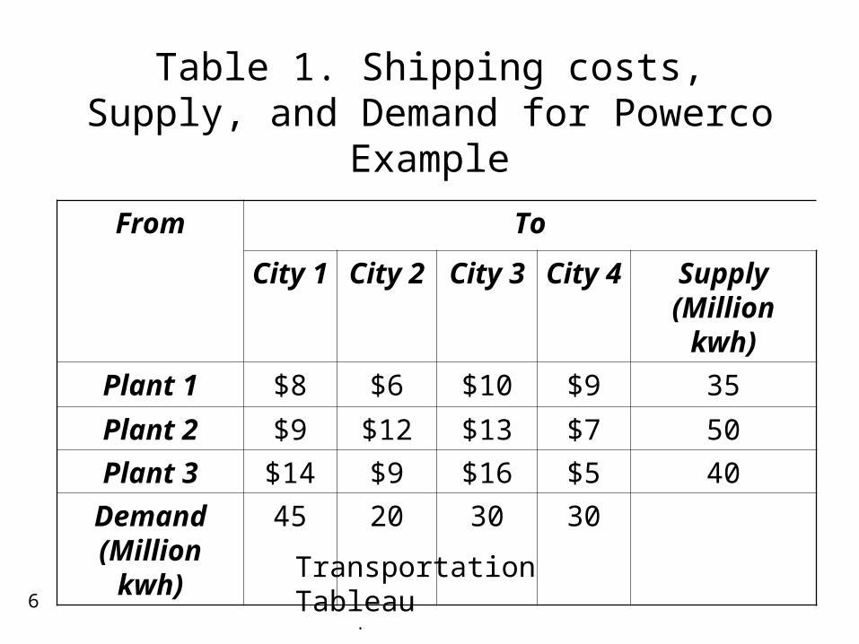
Example 1: Powerco has three electric power plants that supply the electric needs of four cities.•The associated supply of each plant and demand of each city is given in the table 1.•The cost of sending 1 million kwh of electricity from a plant to a city depends on the distance the electricity must travel.

.5

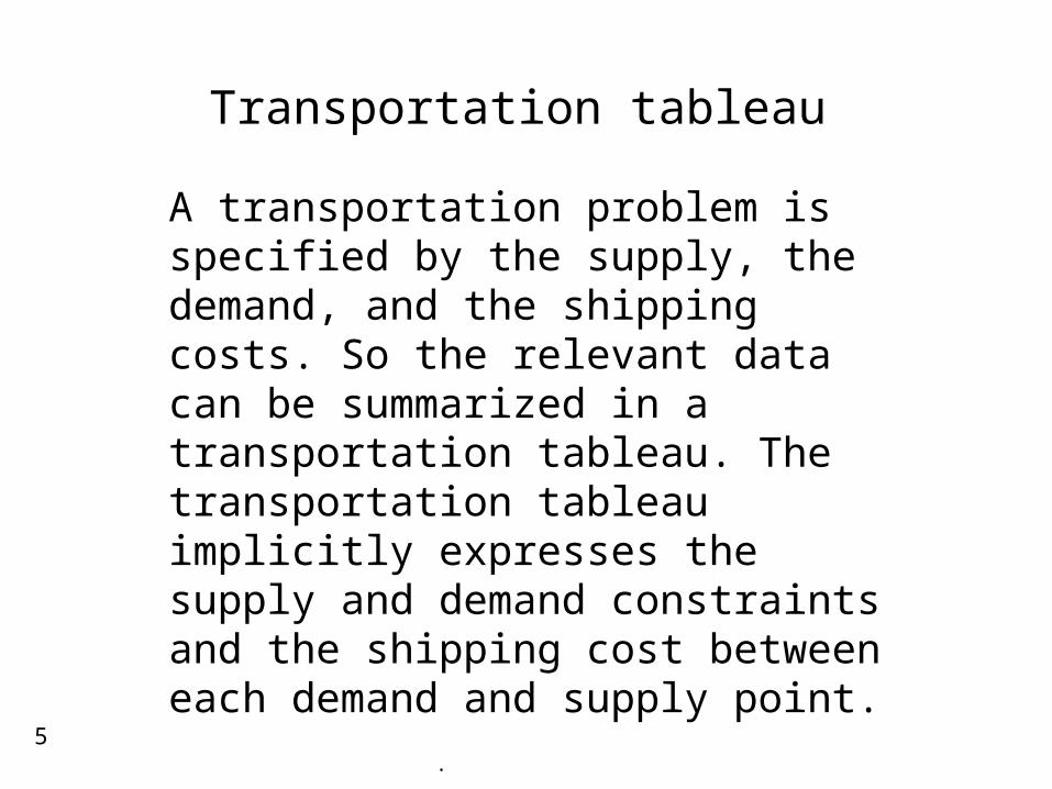
Transportation tableau

A transportation problem is specified by the supply, the demand, and the shipping costs. So the relevant data can be summarized in a transportation tableau. The transportation tableau implicitly expresses the supply and demand constraints and the shipping cost between each demand and supply point.

.6

Table 1. Shipping costs, Supply, and Demand for Powerco Example

From To

City 1 City 2 City 3 City 4 Supply (Million kwh)

Plant 1 $8 $6 $10 $9 35

Plant 2 $9 $12 $13 $7 50

Plant 3 $14 $9 $16 $5 40

Demand (Million kwh)

45 20 30 30

Transportation Tableau

.7

Solution

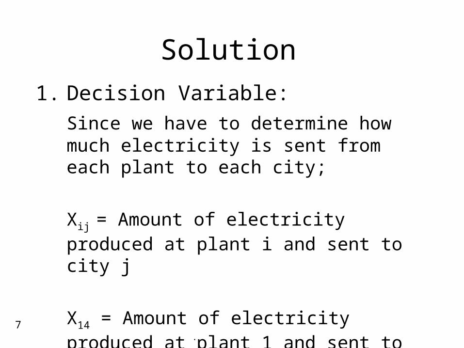
1. Decision Variable:

Since we have to determine how much electricity is sent from each plant to each city;

Xij = Amount of electricity produced at plant i and sent to city j

X14 = Amount of electricity produced at plant 1 and sent to city 4

.8

2. Objective function

Since we want to minimize the total cost of shipping from plants to cities;

Minimize Z = 8X11+6X12+10X13+9X14

+9X21+12X22+13X23+7X24

+14X31+9X32+16X33+5X34

.9

3. Supply Constraints

Since each supply point has a limited production capacity;

X11+X12+X13+X14 <= 35

X21+X22+X23+X24 <= 50

X31+X32+X33+X34 <= 40

.10

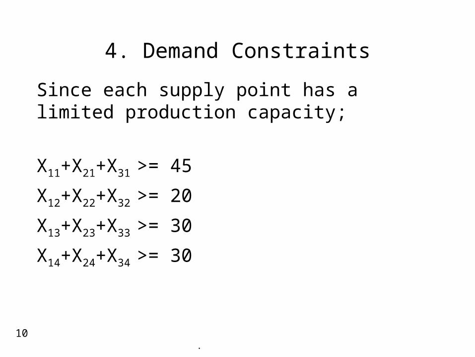
4. Demand Constraints

Since each supply point has a limited production capacity;

X11+X21+X31 >= 45

X12+X22+X32 >= 20

X13+X23+X33 >= 30

X14+X24+X34 >= 30

.11

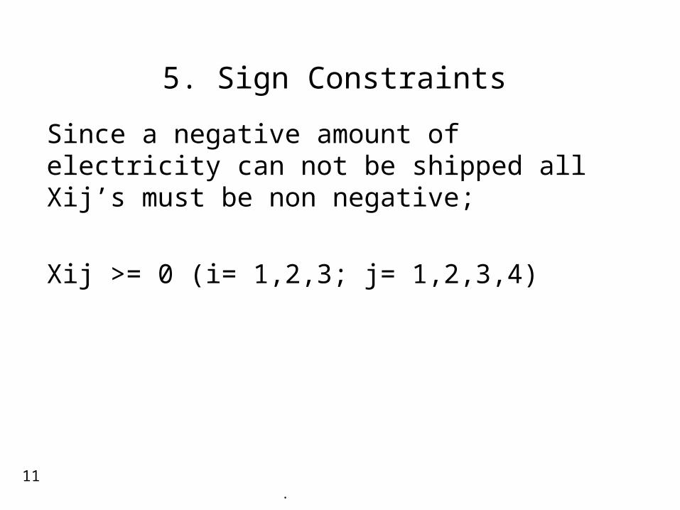
5. Sign Constraints

Since a negative amount of electricity can not be shipped all Xij’s must be non negative;

Xij >= 0 (i= 1,2,3; j= 1,2,3,4)

.12

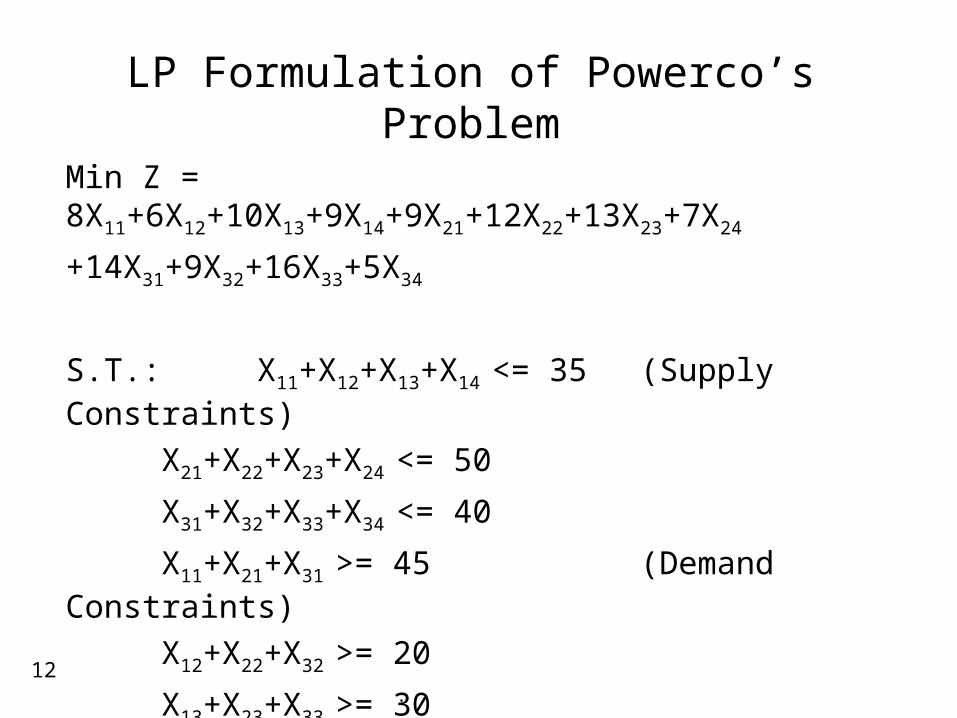
LP Formulation of Powerco’s Problem

Min Z = 8X11+6X12+10X13+9X14+9X21+12X22+13X23+7X24

+14X31+9X32+16X33+5X34

S.T.: X11+X12+X13+X14 <= 35 (Supply Constraints)

X21+X22+X23+X24 <= 50

X31+X32+X33+X34 <= 40

X11+X21+X31 >= 45 (Demand Constraints)

X12+X22+X32 >= 20

X13+X23+X33 >= 30

X14+X24+X34 >= 30

Xij >= 0 (i= 1,2,3; j= 1,2,3,4)

.13

General Description of a Transportation Problem

1. A set of m supply points from which a good is shipped. Supply point i can supply at most si units.

2. A set of n demand points to which the good is shipped. Demand point j must receive at least di units of the shipped good.

3. Each unit produced at supply point i and shipped to demand point j incurs a variable cost of cij.

.14

Xij = number of units shipped from supply point i to demand point j

),...,2,1;,...,2,1(0

),...,2,1(

),...,2,1(..

min

1

1

1 1

njmiX

njdX

misXts

Xc

ij

mi

i

jij

nj

j

iij

mi

i

nj

j

ijij

.15

Balanced Transportation Problem

If Total supply equals to total demand, the problem is said to be a balanced transportation problem:

nj

j

j

mi

i

i ds11

.16

Methods to find the bfs for a balanced TP

There are two basic methods:

1. Northwest Corner Method

2. Vogel’s Method

.17

1. Northwest Corner Method

To find the bfs by the NWC method:

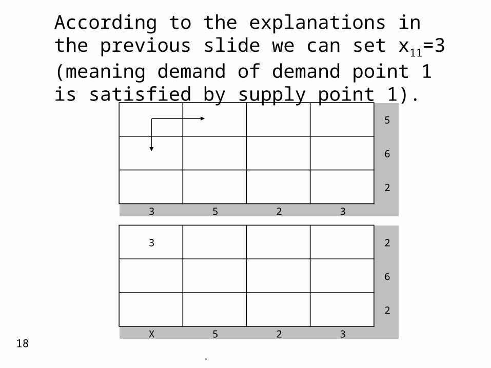
Begin in the upper left (northwest) corner of the transportation tableau and set x11 as large as possible (here the limitations for setting x11 to a larger number, will be the demand of demand point 1 and the supply of supply point 1. Your x11 value can not be greater than minimum of this 2 values).

.18

According to the explanations in the previous slide we can set x11=3 (meaning demand of demand point 1 is satisfied by supply point 1).

5

6

2

3 5 2 3

3 2

6

2

X 5 2 3

.19

After we check the east and south cells, we saw that we can go east (meaning supply point 1 still has capacity to fulfill some demand).

3 2 X

6

2

X 3 2 3

3 2 X

3 3

2

X X 2 3

.20

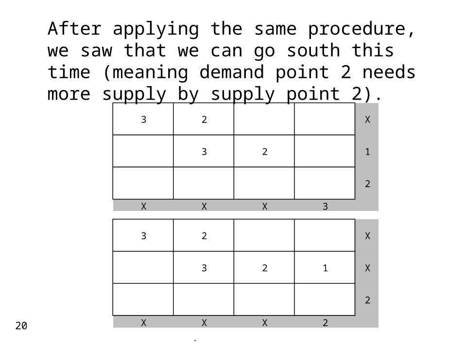
After applying the same procedure, we saw that we can go south this time (meaning demand point 2 needs more supply by supply point 2).

3 2 X

3 2 1

2

X X X 3

3 2 X

3 2 1 X

2

X X X 2

.21

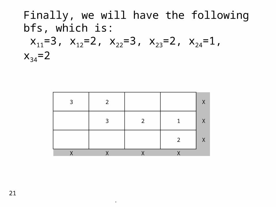
Finally, we will have the following bfs, which is: x11=3, x12=2, x22=3, x23=2, x24=1, x34=2

3 2 X

3 2 1 X

2 X

X X X X

.22

3. Vogel’s Method

Begin with computing each row and column a penalty. The penalty will be equal to the difference between the two smallest shipping costs in the row or column. Identify the row or column with the largest penalty. Find the first basic variable which has the smallest shipping cost in that row or column. Then assign the highest possible value to that variable, and cross-out the row or column as in the previous methods. Compute new penalties and use the same procedure.

.23

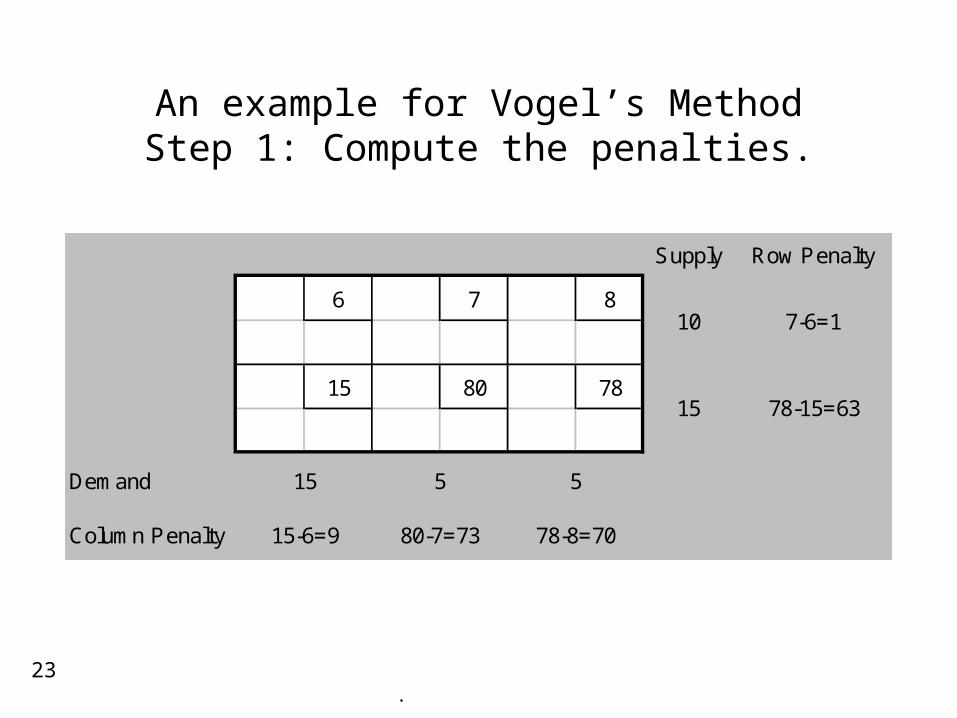
An example for Vogel’s MethodStep 1: Compute the penalties.

Supply Row Penalty

6 7 8

15 80 78

Demand

Column Penalty 15-6=9 80-7=73 78-8=70

7-6=1

78-15=63

15 5 5

10

15

.24

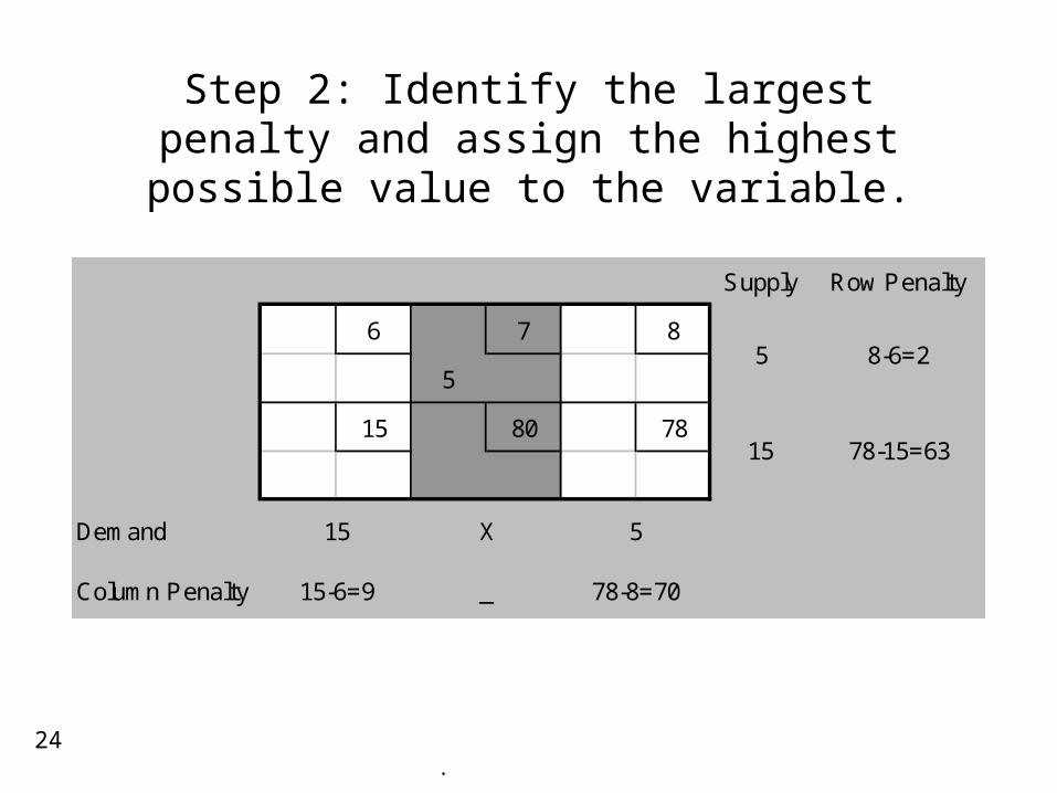
Step 2: Identify the largest penalty and assign the highest possible value to the variable.

Supply Row Penalty

6 7 8

5

15 80 78

Demand

Column Penalty 15-6=9 _ 78-8=70

8-6=2

78-15=63

15 X 5

5

15

.25

Step 3: Identify the largest penalty and assign the highest possible value to the variable.

Supply Row Penalty

6 7 8

5 5

15 80 78

Demand

Column Penalty 15-6=9 _ _

_

_

15 X X

0

15

.26

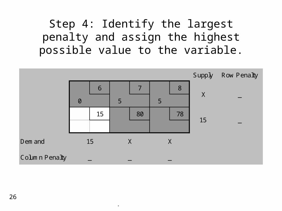
Step 4: Identify the largest penalty and assign the highest possible value to the variable.

Supply Row Penalty

6 7 8

0 5 5

15 80 78

Demand

Column Penalty _ _ _

_

_

15 X X

X

15

.27

Step 5: Finally the bfs is found as X11=0, X12=5, X13=5, and X21=15

Supply Row Penalty

6 7 8

0 5 5

15 80 78

15

Demand

Column Penalty _ _ _

_

_

X X X

X

X

.28

The Transportation Simplex Method

In this section we will explain how the simplex algorithm is used to solve a transportation problem.

.29

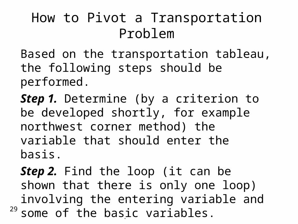
How to Pivot a Transportation Problem

Based on the transportation tableau, the following steps should be performed.

Step 1. Determine (by a criterion to be developed shortly, for example northwest corner method) the variable that should enter the basis.

Step 2. Find the loop (it can be shown that there is only one loop) involving the entering variable and some of the basic variables.

Step 3. Counting the cells in the loop, label them as even cells or odd cells.

.30

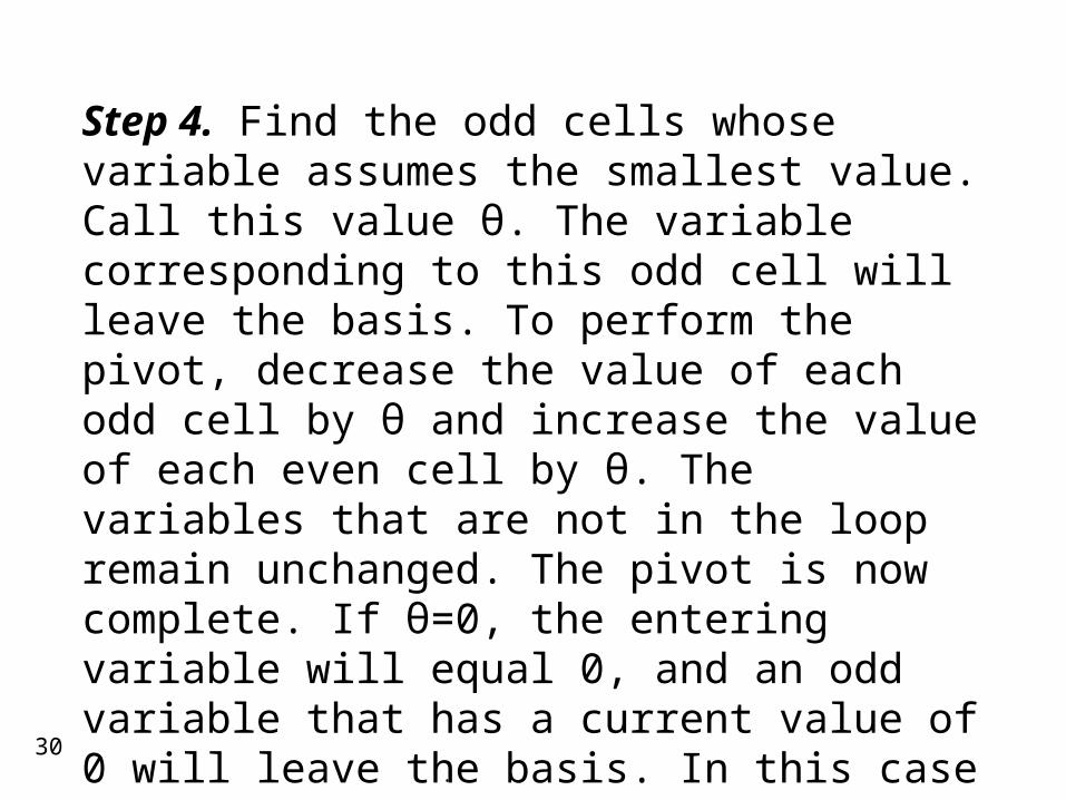
Step 4. Find the odd cells whose variable assumes the smallest value. Call this value θ. The variable corresponding to this odd cell will leave the basis. To perform the pivot, decrease the value of each odd cell by θ and increase the value of each even cell by θ. The variables that are not in the loop remain unchanged. The pivot is now complete. If θ=0, the entering variable will equal 0, and an odd variable that has a current value of 0 will leave the basis. In this case a degenerate bfs existed before and will result after the pivot. If more than one odd cell in the loop equals θ, you may arbitrarily choose one of these odd cells to leave the basis; again a degenerate bfs will result

.31

Assignment ProblemsExample: Machineco has four jobs to be completed. Each machine must be assigned to complete one job. The time required to setup each machine for completing each job is shown in the table below. Machinco wants to minimize the total setup time needed to complete the four jobs.

.32

Setup times

(Also called the cost matrix)

Time (Hours)

Job1 Job2 Job3 Job4

Machine 1 14 5 8 7

Machine 2 2 12 6 5

Machine 3 7 8 3 9

Machine 4 2 4 6 10

.33

The ModelAccording to the setup table Machinco’s problem can be formulated as follows (for i,j=1,2,3,4):

10

1

1

1

1

1

1

1

1..

10629387

5612278514min

44342414

43332313

42322212

41312111

44434241

34333231

24232221

14131211

4443424134333231

2423222114131211

ijij orXX

XXXX

XXXX

XXXX

XXXX

XXXX

XXXX

XXXX

XXXXts

XXXXXXXX

XXXXXXXXZ

.34

For the model on the previous page note that:

Xij=1 if machine i is assigned to meet the demands of job j

Xij=0 if machine i is not assigned to meet the demands of job j

In general an assignment problem is balanced transportation problem in which all supplies and demands are equal to 1.

.35

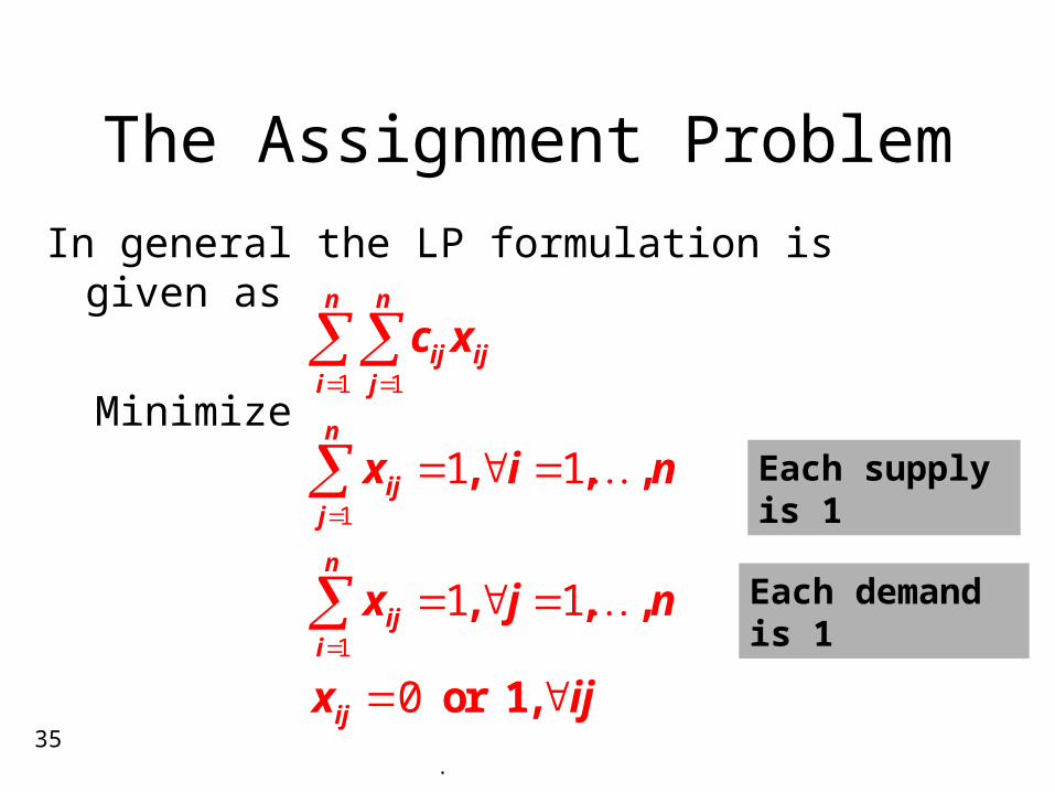
The Assignment Problem

In general the LP formulation is given as

Minimize 1 1

1

1

1 1

1 1

0

, , ,

, , ,

or 1,

n n

ij iji j

n

ijj

n

iji

ij

c x

x i n

x j n

x ij

Each supply is 1

Each demand is 1