© 2000 william w. armstrong breaking hyperplanes to fit data william w. armstrong university of...

© 2000 William W. Armstrong

Breaking Hyperplanes to Fit DataWilliam W. Armstrong

University of Alberta, Dendronic Decisions Limited

Slides of a talk presented at the workshop onSelecting and Combining Models with Machine Learning Algorithms

of the Centre de Recherches MathématiquesMontréal, April 12 – 14, 2000

Thanks to NSERC and DRES for financial support.


Outline of the presentation• Background, definition of ALN• Universal approximation property of ALNs• Growing ALN trees - why depth must be unbounded• Learning -- credit assignment (booleans vs. reals)• Alpha-beta pruning and decision trees for speed • Fillets • Bagging ALNs for improved generalization• Reinforcement learning• Applications• Conclusions


Background• Binary trees that learn boolean functions (1974)• ATREE 2 software distributed (1991)• ALNs compute continuous functions (1993)• Real-time control of a mechanical system (1994)• First commercial ALN product, Atree 3.0 (1995)• Real-time control of a walking prosthesis (1995)• Oxford Univ. Press, IOP : Handbook of Neural

Computation – three articles (1996)• Electrical power load forecasting (1997)• Reinforcement learning (1997)• 3D world modeling for robot navigation (1998)


ALNs• ALNs are piecewise

linear, continuous approximants formed by linear functions and maximum and minimum operators (refinement: fillets smooth the result).

• Main properties:– Universal approximation– Lazy evaluation of f(x)

using few linear pieces for speed

– Ease of interpretation

w xi i

x1 x2 x3 xn...

y Output

Inputs

MAX

MIN

MAX

w xi i w xi i w xi i


y

x

a

b

c

y

x

a

b c

d

y

x

c

b

a

d

e

f

g


ALN approximation of a function without noise.

z = 1000 sin(0.125 x) cos(4 /(0.2 y +1))

x y

z

Error tolerance 0.01, 7 ALNs, ~300 linear pieces per ALN


Universal approximation of a continuous function on a compact set

1. Say function is positive on the compact set (w.l.o.g).

2. For any input x the function value is within ε of f(x)

everywhere in a box at x in input space.

4. Fit function with MAX of the finite set of MINs giving ALN.

3. Form MINs with tops half the size of

the boxes; take finite subcover of

all open half-boxes.

x


Efficient approximation uses curvature of the function graph

MIN =A

MAX=C

MIN=B

Red curve = MIN(MAX(A,B),C)

Many MIN bumps would be needed in place of C


Why deep trees are necessary for fitting with few linear pieces

A B BA

C C

D

MIN(A,MAX(B,MIN(C,D))) whereA is a MIN, B is a MAX, C is a MIN, D is a MAXof linear pieces


ALN smoothing by fillets

Parts of quadratic curves (green) are used to make the function (twice) continuously differentiable. Linear or quartic fillets could also be used.

Input axis

Output axis


Training and tree growth• The weights of the linear functions are changed by

training – like iterative linear regression.• Simple credit assignment for training:

At a MAX (or resp. MIN) node, for a given input, the greater (or resp. lesser) of the two inputs makes its subtree responsible (fillets: both change)

• Alpha-beta pruning speeds up training.• A linear piece splits if, after training, its RMS

error is above an allowed error tolerance. The criterion tends to keep pieces “round” rather than “long” (see Delaunay triangulation comparison).


ALN Learning

Data point pulls (blue arrow)the line from dotted to solid position. Green points no longer influence line.

Input axis

Output axis


Lazy evaluation of an ALN

• A leaf node is evaluated in time T diminput * (multiply-add time) on a serial machine, where diminput is the number of variables in the input.

• Alpha-beta pruning allows an n layer balanced tree to be evaluated in time less than 2T * 1.83(n-2). Complete evaluation is 2n-

1 T. So for n = 10, less than 50% is done.


Lazy training of an ALN• With fillets that are active only ¼ of the

time, an n-layer ALN trains for one sample in time (5/4)(n-1) T1 where T1 is the training time of a linear piece.

• Full training time is 2(n-1) T1 . So for a 10-layer tree, less than 1.5% of the leaves need to be trained for that sample!

• Evaluation is accelerated by having an approximate value of the output.


Logical and real-valued views• Boolean outputs of

simple perceptrons xn wi xi

indicate sets of points under the function graph of a linear piece.

• AND and ORcombine perceptron outputs and represent a real-valued function by the set of points under the function graph.

• Linear functions xn = wi xi

compute real values directly given inputs x1 to xn-1.

• Minimum and maximum combine linear functions and produce real-valued functions


Question:

Was it just the use of boolean values in the early multilayer perceptrons,

instead of real values with their easy credit assignment algorithm, that was responsible for early disappointment

with neural nets in the 1960’s?


ALN Learning (adding linear pieces)

If adapting the linear pieces doesn’t reduce the error of a piece below a given tolerance, then the piece splits into two, each of them starting off equal to the parent.

Input axis

Output axis


ALN Learning(limiting over-fitting)

Does splitting reduce the error on a validation set? Set an error tolerance on the output so that a piece doesn’t split to fit noise.

Input axis

Output axis


Change of ALN output variable if output is monotonic in some input variable (inversion)

MIN becomes MAX in inverse ALN

MAX becomes MIN in inverse

ALN

Output weight is always set to –1by renormalizing.

Increasing case: MAX and MIN interchange.Decreasing case: they don’t.


Fast evaluation after training using an ALN decision tree

1

23

45 6

Input axis x

Min(5,6)Min(4,5)Min(2,3,4)Min(1,2)

For x in this intervalonly pieces 4 and 5 play a role.

x


Method for bagging ALNs• Separate available data into test set and a

combined training-validation set (TV set).• Randomly select n subsets of ~70% the TV set and

train an ALN on each using a fixed error tolerance to control splitting. Note average RMS error on samples not used in training.

• In several trials, seek the error tolerance with the lowest error on samples not used in training.

• Use tolerance found above to train n new ALNs.• Take the average of the n ALNs as approximant.• Test that approximant against the test set.


Error tolerance 100, one ALN, 24 active pieces, very small fillets.


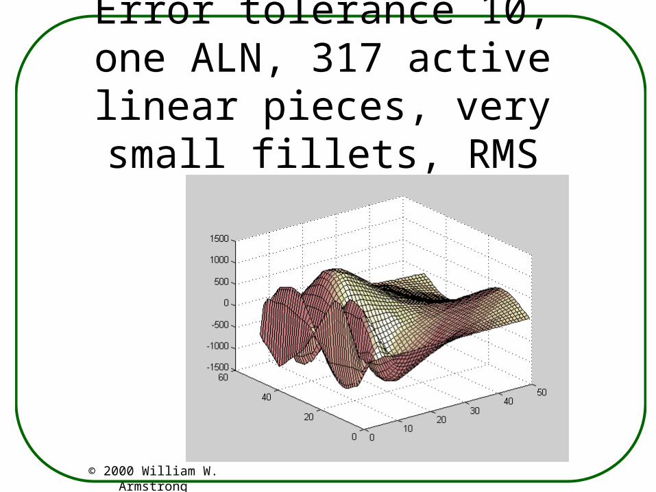
Error tolerance 10, one ALN, 317 active linear pieces, very small fillets, RMS error 23.


Error tolerance 10, seven ALNs, ~ 300 active linear pieces each , very small fillets,

RMS error of average = 12.


Error tolerance 5, twenty-five ALNs, ~ 500 active linear pieces each , very small fillets,

RMS error of average = 8.


Error tolerance 5, twenty-five ALNs, ~ 410 active linear pieces each , maximum fillet ~1,

RMS error of average = 8. Fillets have reduced the number of pieces used by ~18%.


Examples with noise obtained by adding 200*rand()-100 to the original function. The standard deviation of noise which is uniform on [-100,100] is 57.7.


Error tolerance = 100 (the noise amplitude), one ALN, 38 linear pieces, max. fillet 25,

RMS error on test set ~100


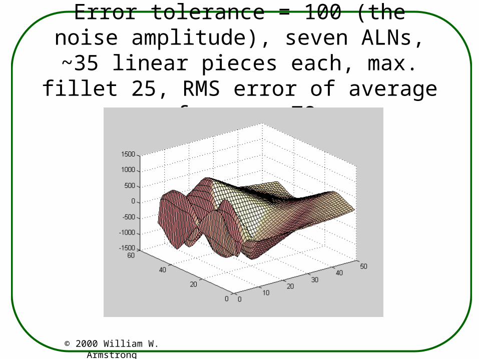
Error tolerance = 100 (the noise amplitude), seven ALNs, ~35 linear pieces each, max.

fillet 25, RMS error of average of seven ~78


Error tolerance = 57.7 (the noise RMS), one ALN, 167 active linear pieces, max. fillet 14.4, RMS error on test ~ 66


Error tolerance = 57.7 (the noise RMS), seven ALNs, ~170 linear pieces each, max. fillet 14.4, RMS error of average of seven ~61(best result on noisy data -- expected best possible: 57.7)


Overtraining: error tolerance = 10 (10% of the noise amplitude), one ALN, 1688 linear

pieces, max. fillet ~3, RMS error 79 on test.


Overtraining: error tolerance = 10, seven ALNs, ~1700 linear pieces each, max. fillet ~3, RMS error 69 on test (using noisy data).


A comparison of the ALN trained on noiseless data (left) to the average of seven ALNs on noisy data f(x) n, n[-100,100] using the noise standard deviation as the error tolerance for ALN splitting (right).


Question: Can we estimate generalization error of a good ALN

using an overtrained ALN?

Delaunay triangulation of training point inputs and approximation of validation set value (red)

Overtrained filleted (blue) ALN fitting six points and approximating validation set value (red).


Some results• Single ALNs slightly worse than weighted

KNN regression on many benchmarks. Good on ship icing problem. (Bullas).

• Pima Indians diabetes database: average of 7 ALNs gave 22.5% error with tolerance 0.4

• Pima Indians again: 25 ALNs, tolerance 0.38, 22% classification error. Final training of 25 ALNs took 65 seconds.


Reinforcement Learning• Some requirements were formulated for a machine

learning system to support Q-learning by Juan Carlos Santamaría, Richard S. Sutton and Ashwin Ram: Experiments with Reinforcement Learning in Problems with Continuous State and Action Spaces, COINS Technical Report 96-088, 1996.

• We have to solve Bellman’s equation Q* (s,a) = r(s,a) + maxa’ Q* (s’,a’) by learning Q* (s,a), the optimal discounted reinforcement of taking action a in state s.


Requirement 1

• The function approximator has to accurately generalize the values of the Q-function for unexplored state-action pairs.

• ALN solution: with ALNs, constraints on weights can be imposed to prevent rapid changes of function values (giving rise to Lipschitz conditions on functions).


Requirement 2• The function approximator has to be able to reflect

fine detail in some parts of the state-action space, while economizing on storage in parts that don’t require detailed description.

• ALN solution: ALN tree growth can accommodate the function in parts of the space requiring more linear pieces, without excessive proliferation in the rest.


Requirement 3• The storage needed to achieve finer resolution should not

cause the approximator to become less usable. In high-dimensional spaces, the method should not suffer from the “curse of dimensionality” by requiring a large number of

approximation units.

• ALN solution: In the case of ALNs, the storage required by a single linear function is proportional to the dimension of the space. The number of linear pieces required to fit the action-value function depends only on the complexity of that function.


Requirement 4• There is a need for computational efficiency.• ALN solution: In the case of ALNs, algorithms

can omit large parts of a computation using alpha-beta pruning. After an ALN has been trained, a decision tree can be used to divide the input space into blocks in each of which only a few linear pieces are active. The number of linear pieces involved on any block can be limited to the number of inputs to the Q-function plus one.


Question: Why does ALN reinforcement learning succeed?

State-action space

Current state-action s,a

Polyhedron of one linear piece: change of its weights need not change Q* (s’,a’)

Values Q* (s’,a’) are used to train Q* (s,a) by Bellman’s equation

Q* (s,a) = r(s,a) + maxa’ Q* (s’,a’)


ALN Applications

• Short term forecasting of electrical power demand in Alberta (for EPCOR)

• Walking prosthesis (with Aleks Kostov†)

• Analysis of oil sand extraction (for ARC)

• Modeling 3D space for robot navigation (for DRES, with Dmitry Gorodnichy)


WEATHERDATA

ACQUISITIONSYSTEM

WEATHERDATAPRE-

PROCESSINGUNIT

WEATHERDATABASE

(HISTORICAL&

FORECAST)

OUTPUT

• Temperature• R.H.• Wind Speed• Cloud Opacity for seven locations in Alberta

• Modem Dialup• Interface

• Data Correction• Data Formatting• C++ Code

• Day of Year• Day of Week• Long Weekends• Holidays• Daylight Saving Time• Twilight Duration

CALENDARDATA

GENERATOR

Short-Term Load Forecast System

ALNDATA

PROCESSINGUNIT

ALNENGINE

• 1 hour• 1 day• 1 week


Alberta SystemThanks to EPCOR

Total Installed Generating Capacity: 7,524 MW (“Peak Continuous Rating”);Number of Generating Units: 64;External Interchange Capacity: 400 MW (1,000 MW export) with BC;

150 MW (DC tie) with SK;Min. Load (1996): 4,300 MW;Peak Load (1996): 7,000 MW;Average Load (1996): 5,500 MW;

BC SK


Day 1 Day 2 Day 34500

5000

5500

6000

6500

7000

Alb

erta

Loa

d [M

W]

Unit A

Unit B

Unit C

Unit D

Unit E

Unit F

Unit G

Marginal Unit Commitment to MeetSystem Peak Demand (Thanks to EPCOR)


Factors Influencing Load

=

Electric Load Population Time Season Weather

+ ++

ConclusionThe load function is non-linear, and difficult to model accurately using traditional mathematical tools.


Sample Results

4200

4600

5000

5400

5800

6200

1 3 5 7 9 11 13 15 17 19 21 23HOUR

MW

ACTUAL

FORECAST

WINTER

SUMMER


Accuracy of ALN for Alberta• Predictions one hour ahead: 0.80 % MAPE*• Predictions 24 hours ahead: 1.17 % MAPE*• Predictions 48 hours ahead: 1.40 % MAPE*

•*MAPE = Mean Absolute Percentage Error

Absolute Percentage Error on the i-th estimate of the load = 100 * | estimated i - actual i | / actual i


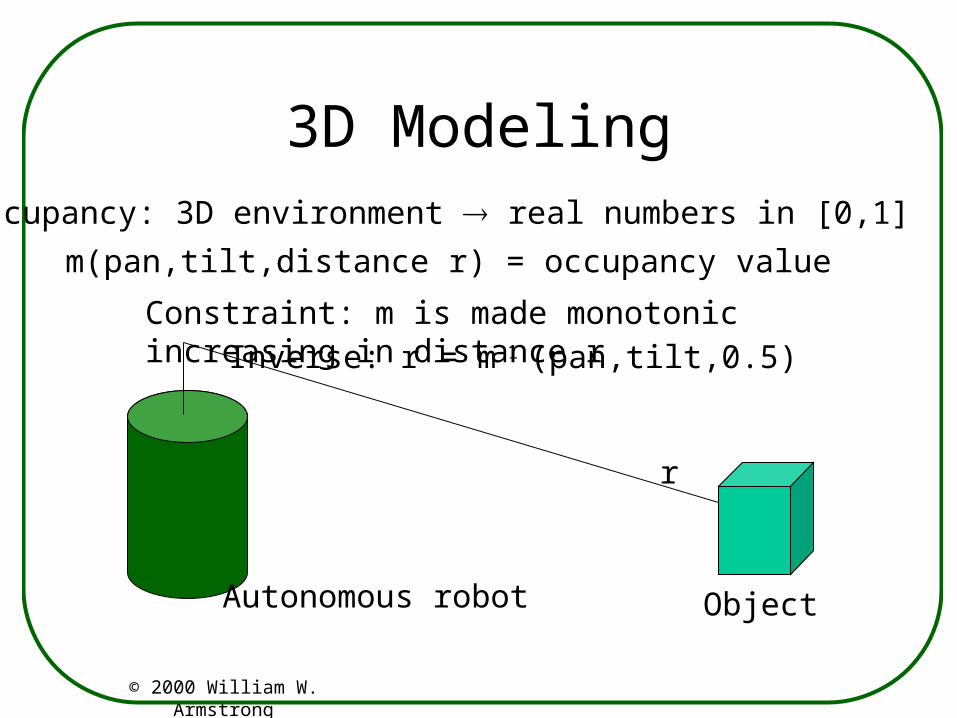
3D ModelingOccupancy: 3D environment real numbers in [0,1]

m(pan,tilt,distance r) = occupancy value

Constraint: m is made monotonic increasing in distance r

r

Inverse: r = m-1 (pan,tilt,0.5)

Autonomous robot Object


Conclusions• Bagging significantly improves ALN generalization.• A single value of error tolerance controlling hyperplane

splitting achieves good generalization. This avoids choosing kernel sizes and shapes for smoothing inputs.

• Overtrained bagged ALNs provide an upper bound of generalization error that can lead to an estimate of noise variance. (Open: noise of varying amplitude.)

• Yet to be implemented on SDK: variable fillet size, inversion with fillets, linear fillet option.

• There are open geometric problems (ALNs vs. curvature).


Free Software• ALNBench spreadsheet program from

http://www.dendronic.com• Interactive parameter setting• Charting learning progress• Statistical evaluation of over-determined

linear pieces• Dendronic Learning Engine SDK for research

purposes from http://www.dendronic.com with C and C++ APIs.

© 2000 william w. armstrong breaking hyperplanes to fit data william w. armstrong university of...

Documents