© 2007

Rambod Hadidi

ALL RIGHTS RESERVED

GENERIC PROBABILISTIC INVERSION TECHNIQUE FOR

GEOTECHNICAL AND TRANSPORTATION ENGINEERING APPLICATIONS

by

RAMBOD HADIDI

A Dissertation submitted to the

Graduate School-New Brunswick

Rutgers, The State University of New Jersey

in partial fulfillment of the requirements

for the degree of

Doctor of Philosophy

Graduate Program in Civil and Environmental Engineering

written under the direction of

Dr. Nenad Gucunski

and approved by

________________________

________________________

________________________

________________________

New Brunswick, New Jersey

May, 2007

ii

ABSTRACT OF THE DISSERTATION

GENERIC PROBABILISTIC INVERSION TECHNIQUE FOR

GEOTECHNICAL AND TRANPORTATION ENGINEERING APPLICATIONS

BY RAMBOD HADIDI

Dissertation Director:

Dr. Nenad Gucunski

A wide range of important problems in civil engineering can be classified as

inverse problems. In such problems, the observational data related to the performance of

a system is known, and the characteristics of the system or the input are sought. There are

two general approaches to the solution of inverse problems: deterministic and

probabilistic. Traditionally, inverse problems in civil engineering have been solved using

a deterministic approach. In this approach, the objective is to find a model of the system

that its theoretical response best fits the observed data. In deterministic approach to the

solution of inverse problems, it is implicitly assumed that the uncertainties in data and

theoretical models are negligible. However, this assumption is not valid in many

applications, and therefore, effects of data and modeling uncertainties on the obtained

iii

solution should be evaluated. In this dissertation, a general probabilistic approach to the

solution of the inverse problems is introduced, which offers the framework required to

obtain uncertainty measures for the solution. Techniques for direct analytical evaluation

and numerical approximation of the probabilistic solution using Monte Carlo Markov

Chains (MCMC), with and without Neighborhood Algorithm (NA) approximation, are

introduced and explained. The application of the presented concepts and techniques are

then illustrated for three important classes of inverse problems in geotechnical and

transportation engineering as application examples. These applications are: Falling

Weight Deflectometer (FWD) backcalculation, model calibration based on geotechnical

instrument measurements, and seismic waveform inversion for shallow subsurface

characterization. For each application, the probabilistic formulation is presented; the

solution is obtained; and the advantages of the probabilistic approach are illustrated and

discussed.

iv

Dedication

To my parents,

For all their unconditional love and support

v

Acknowledgement

This dissertation is the result of many years of work and study. During these

years, I have been guided, accompanied, and supported by many people. These few lines

are my opportunity to acknowledge their contributions.

First, I would like to express my sincere gratitude to Dr. Nenad Gucunski, my

advisor, for his guidance and support. I thank him as well for providing me an

opportunity to grow as a student and an engineer in the unique research environment he

creates. I would also like to thank Dr. Ali Maher, whose steadfast support was greatly

needed and deeply appreciated.

There are no words to express my gratitude to my parents. Although they have

been living thousands of miles away, that has not stopped the wealth of love, support, and

advice they have given me. They will always have a special place in my heart.

The writing of a dissertation may seem as a lonely and isolating experience, yet it

is obviously not possible without the support of numerous people. Thus, my gratitude

goes to many people who directly or indirectly helped me in this journey. Among them

are faculty and staff at department of civil and environmental engineering of Rutgers

University and my colleagues at Paulus, Sokolowski, and Sartor, LLC.

Support and encouragement from my friends have been essential in completion of

this work. Particularly, I’d like to thank Azam and Bahman Kalantari for their kindness,

encouragement, and support. Finally, my thanks go to Parisa Shokouhi as well for the

happy moments we shared at Rutgers.

Rambod Hadidi, January, 2007

vi

Table of Contents

ABSTRACT OF THE DISSERTATION........................................................................ ii Dedication ......................................................................................................................... iv Acknowledgement ............................................................................................................. v Table of Contents ............................................................................................................. vi List of Tables ..................................................................................................................... x List of Illustrations........................................................................................................... xi 1 Introduction.................................................................................................................... 1

Statement of the Problem ................................................................................................ 1 Objectives ........................................................................................................................ 2 Organization .................................................................................................................... 3 References ....................................................................................................................... 5

2 Uncertainties in Measurements .................................................................................... 6 Introduction ..................................................................................................................... 6 Measurement Specification ............................................................................................. 7 Evaluation and Expression of Uncertainties in Measurement......................................... 8

Evaluation of Uncertainty ............................................................................................ 9 Standard Uncertainty ................................................................................................. 10 Combined Standard Uncertainty................................................................................ 11 Expanded Uncertainty................................................................................................ 11 Uncertainty Interval ................................................................................................... 12

Generalized Measurement ............................................................................................. 12 Summary........................................................................................................................ 14 References ..................................................................................................................... 14

3 Probabilistic Approach to Inverse Problems ............................................................ 15 Introduction ................................................................................................................... 15 Elements of Probability Theory..................................................................................... 16

Kolmogorov’s Concept of Probability ....................................................................... 16 Probability Density .................................................................................................... 17 Homogeneous Probability Density............................................................................. 18 Conjunction of Probabilities ...................................................................................... 18 Marginal Probability.................................................................................................. 20 Independent Probabilities .......................................................................................... 20

Probabilistic Formulation of Inverse Problems ............................................................. 20 Model Space and Data Space..................................................................................... 21 State of Information.................................................................................................... 21 A Priori Information................................................................................................... 22 Forward Model .......................................................................................................... 24 General Probabilistic Solution of the Inverse Problem............................................. 25 Probabilistic Solution in the Case of Data and Forward Model with Gaussian Uncertainties .............................................................................................................. 26

Appraisal of the Probabilistic Solution.......................................................................... 28 Central Estimators and Estimators of Dispersion ..................................................... 28 One and Two Dimensional Marginal Probability Densities...................................... 29

Summary........................................................................................................................ 29

vii

References ..................................................................................................................... 30 4 Monte Carlo Evaluation of the Probabilistic Solution ............................................. 31

Introduction ................................................................................................................... 31 Illustrative Example....................................................................................................... 32 Deterministic Solution................................................................................................... 33 Analytical Evaluation of the Probabilistic Solution ...................................................... 34 Direct Sampling Evaluation of the Probabilistic Solution............................................. 36

Monte Carlo Sampling of Probability Distributions.................................................. 37 Markov Chains ........................................................................................................... 39 Metropolis Sampler .................................................................................................... 40 Cascade Metropolis Sampler ..................................................................................... 41 Monte Carlo Markov Chain (MCMC) Sampling of the Solution of Inverse Problems.................................................................................................................................... 42 Appraisal of Results ................................................................................................... 44 Convergence............................................................................................................... 48 Computational Limitations......................................................................................... 50

Direct Sampling Solution Using Approximation of the Likelihood Function .............. 51 Neighborhood Algorithm (NA)................................................................................... 52 Implementation of NA................................................................................................. 54 Voronoi Diagram ....................................................................................................... 55 Stop Criteria............................................................................................................... 56 Monte Carlo Solution Using Neighborhood Approximation ..................................... 57

Matlab® Application Program ...................................................................................... 60 Summary........................................................................................................................ 61 References ..................................................................................................................... 63

5 Application One: Falling Weight Deflectometer Backcalculation .......................... 65 Introduction ................................................................................................................... 65 Background.................................................................................................................... 66

Review of FWD Test Procedure ................................................................................. 66 Review of Current FWD Backcalculation Procedures .............................................. 69

Probabilistic Formulation of FWD Backcalculation ..................................................... 74 Model a Priori Information........................................................................................ 75 Data a Priori Information .......................................................................................... 76 Forward Model .......................................................................................................... 79 Probabilistic Solution................................................................................................. 85 Computational Time................................................................................................... 85

Backcalculation of Synthetic Test Data......................................................................... 86 Synthetic FWD Test Data........................................................................................... 86 Backcalculation of Layer Modulus based on Deflection Bowl Using Linear Static Forward Model .......................................................................................................... 88 Backcalculation of Layer Moduli Based on Deflection Bowl Using Linear Dynamic Forward Model .......................................................................................................... 94 Backcalculation of Layer Moduli Based on Deflection Time History Using Linear Dynamic Time Domain Forward Model .................................................................... 98 Backcalculation of Layer Moduli and Depth to Bedrock Based on Deflection Time History Using Linear Dynamic Forward Model...................................................... 101

viii

Backcalculation of Layer Moduli and Thickness Based on Deflection Time History Using Linear Dynamic Forward Model................................................................... 103 Backcalculation Based on Velocity Time History .................................................... 103

Backcalculation of FWD Test Data............................................................................. 106 FWD Test Results ..................................................................................................... 106 Backcalculation Results ........................................................................................... 107 A Discussion on Data and Modeling Uncertainties................................................. 108

Effect of Considering Dynamic Material Properties of Pavement Layers on Backcalculation Results............................................................................................... 111

Dynamic Moduli and Damping of Pavement Layers ............................................... 111 Numerical Modeling of Dynamic Moduli and Damping.......................................... 115 Backcalculation of Layer Moduli Based on Deflection Time History Using Linear Dynamic Frequency Domain Forward Model ......................................................... 118 Pavement Response with Dynamic Moduli .............................................................. 121

Summary...................................................................................................................... 124 References ................................................................................................................... 125

6 Application Two: Model Calibration Based On Geotechnical Instrument Measurements ............................................................................................................... 128

Introduction ................................................................................................................. 128 Background.................................................................................................................. 130

Project Overview...................................................................................................... 130 Site Conditions ......................................................................................................... 132 Ground Improvement Program................................................................................ 133

Development of Predictive Model and Calibration Measurements............................. 134 Development of Predictive Model ............................................................................ 134 Measurement Results................................................................................................ 138 Initial Model Predictions ......................................................................................... 140 Model Parameters .................................................................................................... 140

Probabilistic Formulation ............................................................................................ 142 Model a Priori Information...................................................................................... 143 Data a Priori Information ........................................................................................ 143 Forward Model ........................................................................................................ 144 Probabilistic Formulation and Solution .................................................................. 144

Calibration Results ...................................................................................................... 145 Summary...................................................................................................................... 149 References ................................................................................................................... 149

7 Application Three: Seismic Waveform Inversion................................................... 150 Introduction ................................................................................................................. 150 Probabilistic Formulation of Waveform Inversion Problem ....................................... 151

Model a Priori Information...................................................................................... 152 Data a Priori Information ........................................................................................ 152 Forward Model ........................................................................................................ 153 Probabilistic Formulation and Solution .................................................................. 154

Synthetic Seismic Experiment..................................................................................... 154 Test Setup ................................................................................................................. 154 Synthetic Waveforms and Forward Model............................................................... 156

ix

Results of Inversion of Synthetic Seismic Test ......................................................... 158 Inversion of Seismic Pavement Analyzer Data ........................................................... 159

Test Setup ................................................................................................................. 159 Experimental Waveforms ......................................................................................... 163 Forward Model ........................................................................................................ 167 Results of Inversion of SPA Data ............................................................................. 167

Summary...................................................................................................................... 171 References ................................................................................................................... 171

8 Closure ........................................................................................................................ 173 Summary and Conclusions .......................................................................................... 173

FWD Backcalculation .............................................................................................. 174 Model calibration..................................................................................................... 175 Seismic Inversion...................................................................................................... 175

Recommendations for Future Research....................................................................... 176 Appendix A: Spectral Element Method for Analysis of Wave Propagation in Layered Media .............................................................................................................. 178

Introduction ................................................................................................................. 178 Spectral Wave Analysis............................................................................................... 181 Spectral Element Formulation ..................................................................................... 183

Two-Node Layer Element......................................................................................... 183 One-Node Half Space Element................................................................................. 186 Assemblage............................................................................................................... 187 Boundary Conditions and Solution of the System For an Impact Load................... 187

Numerical Implementation .......................................................................................... 190 Illustrative Example..................................................................................................... 191 Summary...................................................................................................................... 192 References ................................................................................................................... 193

Curriculum Vitae .......................................................................................................... 194

x

List of Tables

Table 5-1 - Geometrical and material properties used for defenition of finite element model................................................................................................................................. 83

Table 5-2 – Range of layer moduli values used for evaluation of modeling uncertainties using deflection bowls from static analysis. ..................................................................... 89

Table 5-3 - Geometrical and material properties used for development of spectral element results. ............................................................................................................................. 116

Table 5-4 – Modulus and damping values used for numerical evaluation of spectral element analysis. ............................................................................................................. 121

Table 6-1 – Initial material properties used for development of predictive model. ....... 139

Table 6-2 – Numerical values of the best fit model obtained from calibration analysis. 145

Table 7-1- Subsurface profile parameters in the generation of synthetic waveform inversion example. .......................................................................................................... 158

Figure 7-3 – Synthetic waveforms used in the inversion................................................ 158

Table A- 1 – Geometrical and material properties used in the numerical evaluation and verification of the spectral element method [Alkhoury, 2001]. ...................................... 191

xi

List of Illustrations

Figure 3-1 - Illustration of the concept of conjunction of probabilities P andQ , QP ∧ [Tarantola 2005]. ............................................................................................................. 19

Figure 3-2 - Illustration of the probability densities )(mMρ , )(dDρ , and ),( dmρ representing a priori information on model, data, and joint model and data spaces respectively [Tarantola 2005]. ......................................................................................... 23

Figure 3-3 - (left) Forward model with negligible modelization uncertainties (right) and forward model with modeling uncertainties [Tarantola 2005]. ....................................... 25

Figure 3-4 - Representation of the general probabilistic solution of inverse problem as the conjunction of the a priori information, ),( dmρ and information obtained from forward model ),( dmθ . [Tarantola 2005]. ................................................................................... 26

Figure 4-1 - Deflection based modulus determination experiment. ................................. 33

Figure 4-2 - Graphical representation of the probability densities ),( ∆Eρ , ),( ∆Eθ , and ),( ∆Eσ for the modulus determination experiment. It is assumed that Pap 1=Σ and

m001.0=Σ∆ ................................................................................................................... 35

Figure 4-3 - Graphical representation of the probability density )(EEσ for the modulus determination experiment. It is assumed that Pap 1=Σ and m001.0=Σ∆ . ............... 36

Figure 4-4 - The collection randomly generated samples (right) of a probability distribution (left) allow inference of characteristics of underlying probability distribution [Tarantola 2005]. ............................................................................................................. 38

Figure 4-5 - MCMC solution of the deflection based modulus determination experiment. Histogram (top) and kernel density estimate (bottom) of the a posteriori probability density obtained from analysis of 40000 sampled models. .............................................. 48

Figure 4-6 - Typical Voronoi Diagram in two dimensions............................................... 55

Figure 4-7 - Exact plot (top) and neighborhood approximation (bottom) of the likelihood function with 1000 models. Sampled models, as well as corresponding Voronoi diagram are also shown ( m001.0=Σ∆ ). ...................................................................................... 59

Figure 4-8 - Exact plot of ),( PEσ (top) and MCMC solution using neighborhood approximation (bottom) of the modulus determination experiment ................................. 60

Figure 4-9 Histogram of 10000 samples of the one dimensional marginal a posteriori probabilities of (a) modulus and (b) load, and their corresponding kernel density estimates (c and d) ............................................................................................................ 61

Figure 4-10 Snapshot of the input window of ProbInvert, the developed probabilistic inversion application......................................................................................................... 62

Figure 5-1 - Schematics of FWD test setup (top) and Dynatest® model 8000 FWD trailer (bottom)............................................................................................................................. 68

xii

Figure 5-2 - Typical measured loading history (top) and pavement response during FWD test at different offsets (bottom)........................................................................................ 69

Figure 5-3 - Coefficient of variation of deflection from short term repeatability experiments [Benson, Nazarian and Harrison, 1994]. D1 thru D6 indicates different deflection sensors.............................................................................................................. 78

Figure 5-4 – Axisymmetric ABAQUS® Finite Element mesh with absorbing boundary elements for theoretical modeling of FWD test. ............................................................... 79

Figure 5-5 - Time history (top) and frequency spectrum (bottom) of idealized time history wavelet. ............................................................................................................................. 81

Figure 5-6 - Predicted pavement surface deflection time histories from ABAQUS® finite element model................................................................................................................... 84

Figure 5-7 - Response of pavement surface deflection time histories [Alkhoury, 2001]. 84

Figure 5-8 - Synthetic FWD data for no bedrock (top) and shallow bedrock at 2 m below the surface (bottom). ......................................................................................................... 87

Figure 5-9 - Deflection bowls for synthetic FWD data. ................................................... 87

Figure 5-10 - (a, b and c) Kernel density estimates of marginal a posteriori probabilities for the layer moduli obtained from the probabilistic backcalculation of the deflection bowl with the static forward model without considering modeling uncertainties and (d) comparison of the backcalculated deflection bowls for the pavement section with the most probable layer moduli and the observed data........................................................... 90

Figure 5-11 – Histograms and kernel density estimate of the absolute difference between the calculated maximum deflections from dynamic and static analyses at each receiver location and . The area under each density estimate is equal to one unit. The histograms are scaled to fit in the same figure. ................................................................................... 92

Figure 5-12 - (a, b and c) Kernel density estimates of marginal a posteriori probabilities for the layer moduli obtained from the probabilistic backcalculation of the deflection bowl with the static forward model, which includes the modeling uncertainties, and (d) comparison of the backcalculated deflection bowls for the pavement section with the most probable layer moduli and the observed data........................................................... 93

Figure 5-13 - (a, b and c) Kernel density estimates of marginal a posteriori probabilities for the layer moduli obtained from the probabilistic backcalculation of the deflection bowl with the dynamic forward model and (d) comparison of the backcalculated deflection bowls for the pavement section with the most probable layer moduli and the observed data. ................................................................................................................... 95

Figure 5-14 -(a, b and c) Kernel density estimates of marginal a posteriori probabilities for the layer moduli obtained from the probabilistic backcalculation of the deflection bowl with the dynamic forward model with high model and data uncertainty and (d) comparison of the backcalculated deflection bowls for the pavement section with the most probable layer moduli and the observed data........................................................... 97

Figure 5-15 - (a, b and c) Kernel density estimates of marginal a posteriori probabilities for the layer moduli obtained from the probabilistic backcalculation of the deflection time

xiii

history with the dynamic forward model and (d) comparison of the backcalculated deflection time histories for the pavement section with the most probable layer moduli and the observed data. The two time histories are overlapping...................................... 100

Figure 5-16 - (a, b, c and d) Kernel density estimates of marginal a posteriori probabilities for the layer moduli and depth to bedrock obtained from the probabilistic backcalculation of the deflection time histories with the dynamic forward model and (e) comparison of the backcalculated deflection time histories for the pavement section with the most probable layer moduli and the observed data................................................... 102

Figure 5-17 - (a, b, and c) Kernel density estimates of marginal a posteriori probabilities for the layer moduli obtained from the probabilistic backcalculation of the velocity time histories with the dynamic forward model and (d) comparison of the backcalculated velocity time histories for the pavement section with the most probable layer moduli and the observed data............................................................................................................. 105

Figure 5-18 - Measured loading history (top) and pavement response for FWD test. ... 107

Figure 5-19 -(a, b, and c) Kernel density estimates of marginal a posteriori probabilities for the layer moduli obtained from the probabilistic backcalculation of the experimental deflection time histories with the dynamic forward model and (d) comparison of the backcalculated deflection time histories for the pavement section with the most probable layer moduli and the observed data. ............................................................................... 109

Figure 5-20 - Measured velocity time history record at receiver at zero offset.............. 110

Figure 5-21 - Variation of modulus (top) and damping (bottom) with shear strain for sands [Seed et. al. 1986]. Error! Objects cannot be created from editing field codes. indicates the ratio of the modulus at each frequency to the static modulus......................................... 112

Figure 5-22 - Typical modulus master curves for different asphalt mixtures [Clyne et. al. 2003]. .............................................................................................................................. 114

Figure 5-23 - Predicted pavement surface deflection time histories from linear spectral element analysis. ............................................................................................................. 117

Figure 5-24 - Comparison of predicted surface defections at different receiver location from time domain and frequency domain models. ......................................................... 118

Figure 5-25 - (a, b and c) Kernel density estimates of marginal a posteriori probabilities for the layer moduli obtained from the probabilistic backcalculation of the deflection time history with the spectral element forward model and (d) comparison of the backcalculated deflection time histories for the pavement section with the most probable layer moduli and the observed data...................................................................................................... 120

Figure 5-26 – Sample modulus curve and constant modulus line used for numerical evaluation of the pavement response with spectral element approach. The curve parameters are 8.2=α , 44.0−=β , 48.1−=δ , , 56.0−=γ and 0=TS (See equation 5-4). .................................................................................................................................... 122

Figure 5-27 - Predicted pavement surface deflection time histories from spectral element analysis with dynamic asphalt layer modulus................................................................. 122

xiv

Figure 5-28 - Predicted pavement surface deflection time histories from nonlinear spectral element analysis................................................................................................. 123

Figure 6-1 – Sketch of the generalized subsurface profile ............................................. 133

Figure 6-2 – Total layer settlement for waste, organic site/peat and clay strata. E1-7 and E1-2 are the installed extensometers along the modeled cross section. ......................... 135

Figure 6-3 – Geometry of developed finite element predictive. ..................................... 136

Figure 6-4 – Fill placement timeline at two points along the cross section and idealized fill placement timeline and stages used for model development. ................................... 137

Figure 6-5 – Close up view of idealized loading stages. ................................................ 137

Figure 6-6 – Total layer settlement for waste, organic silt/peat and clay strata from extensometer measurements along the modeled cross section (Extensometer E1-2 and E1-7). .................................................................................................................................... 138

Figure 6-7 – Comparison of observed vs. calculated total layer settlement based on initial layer properties for waste, organic silt/peat and clay strata. ........................................... 141

Figure 6-8 - Comparison of observed vs. calculated total layer settlement based on calibrated layer properties for waste (top), organic silt/peat (middle) and clay (bottom) strata................................................................................................................................ 147

Figure 6-9 - One-dimensional kernel density estimates of marginal probability densities of model parameters for permeability of waste (a), organic sit/peat (b), and clay (c) layer. Similar information is also presented for the compression index of waste (d), organic sit/peat (e), and clay (f) layer. ......................................................................................... 148

Figure 7-1 - Schematics of the synthetic seismic waveform inversion test setup .......... 155

Figure 7-2 - Finite element model with the test setup superimposed on the mesh......... 157

Figure 7-3 – Synthetic waveforms used in the inversion................................................ 158

Figure 7-4 - (a, b, c , d and e) Kernel density estimates of marginal a posteriori probabilities for the layer compressional wave velocities. ............................................. 161 Figure 7-5 - (a, b, c , and d) Two dimensional kernel density estimates of marginal a posteriori probabilities for the layer compressional wave velocities.............................. 162

Figure 7-6 – Schematics of SPA..................................................................................... 160

Figure 7-7 –A/D counts from accelerometers A1, A2, A3, and the high frequency hammer from a test on a flexible section. ....................................................................... 165

Figure 7-8 – Hamming window function and A/D counts from accelerometers A1, A2, A3 after the windowing operation. ................................................................................. 166

Figure 7-9 – - Kernel density estimates of marginal a posteriori probabilities for the layer thickness (a and b) and layer moduli (c, d, and e) obtained from the probabilistic inversion of the acceleration time histories. ................................................................... 169

Figure 7-10 – Comparison of the acceleration time histories for the pavement section with the most probable layer moduli and the observed data........................................... 170

xv

Figure A-1 - Two-node axi-symmetrical layer element [Alkhoury, 2001]..................... 184

Figure A-2 - One-node axi-symmetrical half space element. [Alkhoury, 2001]. ........... 187

Figure A-3 – Spatial distribution of the load [Alkhoury, 2001]. .................................... 188

Figure A-4 - Time history of the idealized time wavelet................................................ 188

Figure A-5 - Frequency spectrum of the idealized wavelet. ........................................... 189

Figure A-6 – Coefficients of Fourier-Bessel series for a circular load of a radius ma 15.0= . ...................................................................................................................... 190

Figure A-7 - Predicted pavement surface deflection time histories from the spectral element analysis. ............................................................................................................. 192

Figure A-8 - Predicted pavement surface deflection time histories from the spectral element analysis [Alkhoury et al.,2001]. ........................................................................ 192

1

1 Introduction

Statement of the Problem A wide range of tasks in civil engineering includes solution of inverse problems.

In such problems, the observational data regarding the performance of a system is known

and the information about the system is sought. Examples of inverse problems in civil

engineering are interpretation of geophysical and nondestructive test data, determination

of material constitutive parameters from laboratory or field data, earthquake location

estimation, and interpretation of geotechnical instrumentation readings.

There are two general approaches to the solution of inverse problems:

deterministic and probabilistic approaches. In deterministic approach to inverse

problems, which has been historically used for applications in civil engineering

[Santamarina, Fratta, 1998], the objective is to find the model of a system that its

theoretical response best fits the observed data. The obtained best fit model is then

generally chosen to represent the inverse problem solution. This approach provides a

single model as the solution of the problem, meaning that no uncertainty in the observed

data or in the theoretically calculated model predictions is considered. However, data and

2

modeling uncertainties are always present, and their effect on the obtained results should

be evaluated. Additionally, there are many situations, where there is information about

the expected results prior to the solution of the inverse problem. For example, this

information can be in the form of the limits of expected values or general trend of the

results. Such information is important and should be included in the solution of the

inverse problem.

The probabilistic approach to the solution inverse problems, which is a new

approach in civil engineering, provides the framework required for obtaining the solution

of the inverse problem and offers mathematical techniques to include prior information

about the solution and to evaluate uncertainty measures [Tarantola, 2005]. The

introduction and application of the probabilistic approach to problems in civil

engineering is the main focus of this research.

Objectives The objectives of this research are:

• introduction of the probabilistic approach to the solution of inverse,

• presentation of the required mathematical background,

• development of computational tools required for the implementation of the

approach, and

• illustration of its application and advantages for the solution of inverse

problems in geotechnical and transportation engineering.

3

Three inverse problems in geotechnical and transportation engineering were

selected as application examples. These problems are:

• Falling Weight Deflectometer (FWD) backcalculation,

• Model calibration based on geotechnical instrument measurements, and

• Seismic waveform inversion.

Organization Following the introduction, the concept of uncertainty in the solution of inverse

problems is formally introduced in chapter two, and its importance is highlighted.

In chapter three, the probabilistic solution of inverse problems is introduced as the

main tool in evaluation of uncertainties in the solution of inverse problems. An overview

of the major concepts used in probabilistic approach is then provided and the

mathematical formulation for the probabilistic solution is presented in general terms

using the introduced concepts.

Chapter four presents several techniques for numerical evaluation of the

probabilistic solution. In this chapter, direct application of the developed formulation for

simple problems is discussed. For complex problems that direct application of the

developed formulation is not feasible, a numerical technique for the solution of the

problem using Monte Carlo Markov Chains (MCMC) is introduced and explained. To

further reduce computational time of obtaining a solution for complex problems, the

introduced MCMC technique is integrated with the recently developed Neighborhood

4

Algorithm (NA) to obtain an approximation to the probabilistic solution. Details of

integration of NA with MCMC are presented, discussed, and explained in this chapter.

Chapters five through seven provide the application examples. In chapter five,

FWD backcalculation problem is considered. The probabilistic formulation of this

problem is introduced and the results of probabilistic backcalculation of synthetic and

experimental data are presented. Using the synthetic test data, different approaches to

backcalculation, such as backcalculation using deflection bowl or time history records,

are studied and compared. The results of these comparisons are also presented in this

chapter.

In chapter six, a brownfield redevelopment project is used as an example to

demonstrate how the probabilistic approach to the solution of inverse problems can be

used to calibrate a predictive model and complement the application of the observational

method in geotechnical engineering. In this chapter, an overview of the mentioned

brownfield redevelopment project is provided and the results of the calibration of a

settlement prediction model using the probabilistic approach are presented and discussed.

Chapter seven presents the probabilistic approach to inversion of the seismic

waveforms for evaluation of soil and pavement layer moduli and thicknesses. The

probabilistic formulation of this problem is introduced and the results of probabilistic

backcalculation of synthetic and experimental data are presented.

Finally, chapter eight provides the summary of the research and offers

recommendations for future research.

5

References Santamarina, J. C. and Fratta D. (1998), “Introduction to Discrete Signals and Inverse

Problems in Civil Engineering”, ASCE Press, Reston, VA. Tarantola, A. (2005), “Inverse Problem Theory”, SIAM, Philadelphia, PA.

6

2 Uncertainties in Measurements

“To measure is to know.”

Lord Kelvin (1824-1907)

Introduction In comparison to the traditional deterministic approach, the main advantage of the

probabilistic approach to the solution of inverse problems is its ability to quantify the

uncertainties of the obtained results. Evaluation of these uncertainties requires a

probabilistic representation of uncertainties of the input parameters of an inverse

problem. Therefore, to provide the required background, the concept of uncertainty is

formally introduced in this chapter.

The concept of uncertainty, as it relates to direct physical measurements, is a very

familiar and accepted concept in engineering. In simple terms, it is a representation of the

likely values of the measurement results. The concept of uncertainty is sometimes

confused with the concept of error. Error refers to the difference between the true value

of the quantity subject to measurement, called measurand, and the measurement result. A

measurement can unknowingly be very close to the unknown value of the measurand,

thus having a negligible error; however, it may have a large uncertainty. Since the exact

value of a measurand can never be evaluated, error is an abstract concept, which can

7

never be quantified. However, uncertainty is a measure that can be and should be

quantified for every measurement.

The probabilistic presentation of uncertainties in direct measurements is

formalized by International Organization for Standardization (ISO) and United States

National Institute of Standards and Technology (NIST) [ISO, 1993, Taylor and Kuyatt,

1994]. According to the recommendations of ISO and NIST, measurement uncertainties

should be expressed explicitly using probabilistic concepts. This presentation is the first

step towards the implementation of the probabilistic approach to the solution of inverse

problems, where the direct physical measurements are one of the inputs to the problem.

In this chapter, important ISO and NIST concepts and guidelines for presentation

of uncertainties in direct measurements are reviewed. Following this review, the notion of

measurement is generalized to include indirect measurement of physical quantities in

inverse problems. It is shown that using this generalized notion, any inverse problem can

be viewed as a measurement, which its uncertainties should be evaluated. Such

evaluation can be accomplished using a probabilistic approach to the solution of inverse

problems. Therefore, the probabilistic approach can be considered as an extension of

NIST and ISO guidelines to include generalized measurements.

Measurement Specification The first step in making a measurement is to specify the measurand. The

specification of a measurand, which specifies how the measurement should be carried

out, is directly related to the required accuracy of the measurement. For example, if the

length of a bar is to be determined with micrometer accuracy, its specification should

8

include the temperature and pressure at which the measurement is supposed to be carried

out. The uncertainty of the length measurement, if temperature and pressure are not

specified, is so high that micrometer accuracy can not be achieved, even if the accuracy

of the measurement instrument is adequate. Theoretically, it is possible to find the

minimum level of uncertainty attainable for any given measurement specification.

However, in most practical applications, the minimum level is not usually achieved. The

measurement specification and the associated minimum level of uncertainty attainable

should be always considered in interpretation of measurement results, even when no

uncertainty measure is provided.

Evaluation and Expression of Uncertainties in Measurement Once a measurement is carried out according to a given specification, the

associated measurement uncertainties arising from different source of uncertainty should

be evaluated, combined, and expressed with the measurement results. Sole presentation

of the measurement value without any uncertainty measure does not provide the complete

picture and might be misleading. ISO and NIST [ISO, 1993, Taylor and Kuyatt, 1994]

provide general recommendation for expressing uncertainties in direct physical

measurements. These recommendations form a basis for probabilistic expression of

measurement uncertainties, which can be directly used in the probabilistic approach to

the solution of inverse problems. This section presents the major concepts and

recommendation of NIST, which for the most part are adopted from ISO.

9

Evaluation of Uncertainty

In the NIST approach, any source of uncertainty in the measurement is

categorized in two classes based on the method used for its evaluation:

• Type A Uncertainties: Uncertainties that are evaluated by statistical methods

• Type B Uncertainties: Uncertainties that are evaluated by other means

Evaluation of “Type A” uncertainties is based on any valid statistical method,

such as evaluation of the mean and standard deviation of a series of measurements or by

performing analysis of variances (ANOVA). For example, uncertainties of measurement

instruments provided by manufacturer’s specifications or calibration reports are generally

evaluated as “Type A” uncertainties.

A “Type B” evaluation is based on non statistical evaluation, such as subjective

evaluation based on scientific or engineering judgment, previous measurement data,

experience with or general knowledge of the behavior of the instrument and measurand,

and information published in reference books and handbooks.

Most sources of uncertainty can be evaluated either as a Type A or a Type B

uncertainty. For example, the uncertainty in a measurement due to a change of the

observers can be evaluated statistically with analysis of a series of observations from a

group of independent observers, or it can be simply evaluated as a Type B using the

previous experience and judgment for that type of measurement.

It should be mentioned that NIST’s classification of uncertainties is different than

the traditional classification that divides uncertainties into “random” and “systematic”.

10

There is not always a simple one to one correspondence between these two

classifications. Depending on how the measured quantity is used in mathematical

equations, a random uncertainty arising from a random effect may become systematic

and vice versa. For example, the uncertainty in a correction value applied to a

measurement result to compensate for a systematic effect can produce a random or

systematic uncertainty.

In routine engineering applications, direct statistical evaluation of the

measurement uncertainties from all sources of uncertainty is not generally feasible and

some of the measurement uncertainties should be evaluated as a Type B uncertainty. For

example, in the measurement of settlement, in addition to uncertainty of measurement

instrument, uncertainties in the measurement process due to other factors, such as

uncertainty in positioning of instruments, or uncertainties due to change of the observer

should also be evaluated and included in the uncertainty measure.

Standard Uncertainty

In NIST approach, the basic quantity representing uncertainty (Type A or B) from

a single source is the standard uncertainty, denoted by symbol s , which is the standard

deviation of the measurement when only one source of uncertainty is considered. In this

representation, a Gaussian distribution for the source of uncertainty is implicitly

considered and it is quantified by the value of the standard deviation.

11

Combined Standard Uncertainty

A measurement is usually subject to uncertainties from different sources. Ideally,

the standard uncertainty should be evaluated for each source of uncertainty in the

measurement as a Type A or a Type B uncertainty and then combined together to provide

a single uncertainty measure. In other words, if all the uncertainties in the measurement

process are characterized by standard uncertainties is , these individual uncertainties

should be combined to represent combined standard uncertainty, cs , of the measurement.

Such combination can be obtained by calculating the square root of the sum of the

squares of individual standard uncertainties is . This method, which is based on the

probability theory, is sometimes referred to as law of propagation of uncertainty. The

combined standard uncertainty is the quantity reported as the uncertainty in

measurements.

Expanded Uncertainty

The combined standard uncertainty is the main quantity used in presentation of

the measurement results. However, NIST also recognizes the presentation of uncertainty

as expended uncertainty in the form of Sdobs ± , where obsd is the measured value and S

is half of the uncertainty interval. The relationship between expanded and standard

uncertainty is presented by cksS = , where cs is the combined standard uncertainty and

k is called the coverage factor. Typically k is between 2 and 3. Assuming a Gaussian

distribution, 2=k defines an interval with a confidence level of 95 percent, whereas

3=k defines a interval with a confidence level of 99 percent.

12

Uncertainty Interval

Uncertainties of measurements are also sometimes specified in the form of

uncertainty interval, where for a given measurement, the upper and lower limits of the

measurement value are identified. In such cases, given the upper and lower limits of the

measurement result, denoted by upperd and lowerd , the uncertainty can be calculated by

assuming the best estimated value as 2/)( lowerupper dd + and calculating a corresponding

combined standard uncertainty for the measurement, cs . The combined standard

uncertainty is then calculated such that there is a certain probability that the measurement

result is between upperd and lowerd . For example, for a 50 percent probability

choose 2/)(48.1 lowerupperc dds −= , for a 67 percent probability select

2/)( lowerupperc dds −= ,and for a 99 percent probability use 3/)( lowerupperc dds −= .

NIST also presents guidelines to convert uncertainties stated in other forms to

combined standard uncertainty. A detailed account of these guidelines is provided in the

cited references [Taylor and Kuyatt, 1994].

Generalized Measurement In general, a measurement is considered to be a direct evaluation of a quantity

subject to measurement. An inverse problem on the other hand is an indirect evaluation

of the parameters of interest in the problem through measurement of another set of

parameters and using the theoretical relationships between these two sets of parameters.

Since the ultimate objective of an inverse problem is also measurement of the parameters

13

of interest in the problem, an inverse problem can also be considered a complex and

indirect measurement using physical theories [Tarantola, 2005]. Such a measurement is

referred to here as a generalized measurement. In principle, there is no difference

between a direct measurement and a generalized measurement. In fact, the measurements

that are considered direct measurements are simple forms of inverse problems. For

example, measurement of the weight by a spring scale is a simple direct measurement,

which can be considered a simple inverse problem. In this problem the parameter of

interest is the weight of an object, which is evaluated indirectly by measurement of the

deflection of a spring. In this example, the physical theory linking the observed parameter

(deflection) to the parameter of interest (weight) is a very simple linear relationship. The

solution of the problem is trivial, which is often solved using a calibrated gauge.

Similar to direct measurements, there are uncertainties associated with any

generalized measurement. These uncertainties are basically due to uncertainties in

physical measurements and uncertainties inherent in physical theories that are used in

generalized measurements. These uncertainties should be evaluated and presented with

the results of generalized measurements. However, evaluation of these uncertainties can

not be performed using the NIST guidelines. Since the NIST approach deals with direct

measurements only, there is a great emphasis on the use of Gaussian probabilities for

expression of uncertainties. Although use of Gaussian probabilities is very appropriate for

representing uncertainties in direct measurements, they can not in general represent

uncertainties in generalized measurements, where the uncertainty may follow other

distributions. The probabilistic approach to the solution of inverse problems provides the

required tools to evaluate uncertainties in generalized measurements. In this sense, the

14

probabilistic approach to solution of inverse problems can be considered as an extension

of NIST and ISO guidelines to include generalized measurements.

Summary Basic and established guidelines in the presentation of uncertainties in direct

measurements were introduced and reviewed in this chapter. These guidelines are the

first step towards the probabilistic solution of the inverse problems, where the simple

physical measurements are one of the inputs to the problem. The notion of inverse

problem as a generalized measurement was also introduced in this chapter. It has been

stated that using this generalized notion, any inverse problem can be viewed as a

measurement, which its uncertainties should be evaluated and presented with the

measurement result. In this sense, the probabilistic approach to solution of inverse

problems can be considered as an extension of NIST and ISO guidelines to include

generalized measurements.

References International Organization for Standardization (1993), “Guide to the Expression of

Uncertainty in Measurement”, International Organization for Standardization, Geneva, Switzerland.

Tarantola, A. (2005), “Inverse Problem Theory”, SIAM, Philadelphia, PA. Taylor B. N. and Kuyatt C. E. (1994), “Guidelines for Evaluation and Expressing

Uncertainty of NIST Measurement Results”, Technical Note 1297, United States National Institute of Standards and Technology (NIST), United States Department of Commerce, Washington, DC.

15

3 Probabilistic Approach to Inverse Problems

“Far better an approximate answer to the right question, which is often vague, than the exact answer to the wrong question, which can always be made precise.”

John Tukey, Statistician (1915-2000)

Introduction Inverse problem is a mathematical problem where the objective is to obtain

information about a parameterized system (i.e. model) from observational data,

theoretical relationships between system parameters and data, and any available a priori

information. The most general form of the inverse problem theory is obtained using a

probabilistic point of view, where the a priori information on the problem parameters and

theoretical relationships is represented by probability distributions. In this approach, the

solution of the inverse problem is itself a probability distribution representing the

combined information about model parameters and theoretical relationships. The inverse

problem solution with probabilistic approach in simple cases will reduce to the same

solution obtained from the traditional deterministic approach. However, with this

approach, more information about the solution is obtained and more complex inverse

problems can be solved.

This chapter provides an introduction to the mathematical theory of inverse

problems from a probabilistic point of view. This introduction is mainly based on the

formulation of the theory presented by Tarantola [Tarantola 2005, Mosegaard and

Tarantola 2002, Tarantola 2004, Tarantola and Valette 1982]. Following this

16

introduction, elements of probability theory required in formulating the probabilistic

solution are initially introduced. General probabilistic approach to inverse problems is

then formulated, solution of the problem is defined, and common techniques for appraisal

of the solution are introduced. Due to introductory nature of the chapter, there has been a

conscious effort to present the main ideas and important results with less emphasis on

mathematical derivations and proofs. Interested readers can find a detailed mathematical

treatment of the subject in the cited references.

Elements of Probability Theory Probability theory is essential to the probabilistic formulation of inverse problems

presented here. Therefore, this section contains a review of the elements of probability

theory which are important for the analysis of inverse problems.

Kolmogorov’s Concept of Probability

The Kolmogorov’s [1933] definition of probability, clarifies the underlying

mathematical structure of probability and allows a formal presentation of the concepts

based on which the probabilistic solution of inverse problems are based.

Consider a point x that can be materialized anywhere inside a space of points

denoted as χ . The point x may for example be realized in the domain A of χ ( χ⊂A ).

The probability of realization of a point can be completely described, if to every domain

A of χ a positive number )(AP can be assigned having three properties:

• For any domain A of χ , 0)( >AP .

17

• If iA and jA are two disjoint domains of χ , then

)()()( jiji APAPAAP +=∪ .

• If domainEmptyA → , then 0)( >AP .

The )(AP , which satisfies the above criteria, is called the probability of A and

defines a probability distribution over χ . It should be mentioned that in this definition, it

is not assumed that the probability is necessarily normalized to unity (i.e. 1)( =χP ). If

the probability is not normalized, it is sometimes referred to as a measure. Some

probabilities are not normalizable (i.e. ∞=)(χP ). In such cases, only relative

probabilities can be computed.

Generally, any type of coordinate system can be selected to represent points in

space χ ; however, for most applications, including for the applications considered in this

work, the Cartesian coordinate system is the most convenient system. The formulation of

probabilistic approach presented here assumes that the Cartesian coordinates are the

coordinates used to define the problem. In special cases where the coordinates are not

Cartesian, the presented formulation should be slightly modified [Tarantola 2005].

Probability Density

A probability distribution, )(AP , can also be represented by its probability

density function, )(xp , which is defined as:

∫=A

xxpAP δ)()( (3-1)

18

where nxxxx δδδδ ...,21= is a volume element.

Homogeneous Probability Density

The homogeneous probability distribution is a probability distribution that assigns

to each domain of the space a probability proportional to its volume or:

)()( AkVAM = (3-2) where )(AM represents the homogenous probability distribution, k is a proportionality

constant, and )(AV is the volume of A of χ , which is defined as:

∫=A

xAV δ)( (3-3)

Combining equations (3-1), (3-2) and (3-3), it is easy to show that density

function of homogenous probability density denoted by )(xµ is:

kx =)(µ (3-4) where k is a constant. It should be remembered that in coordinate systems other than

Cartesian coordinate system, the homogeneous probability density may not be constant.

Conjunction of Probabilities

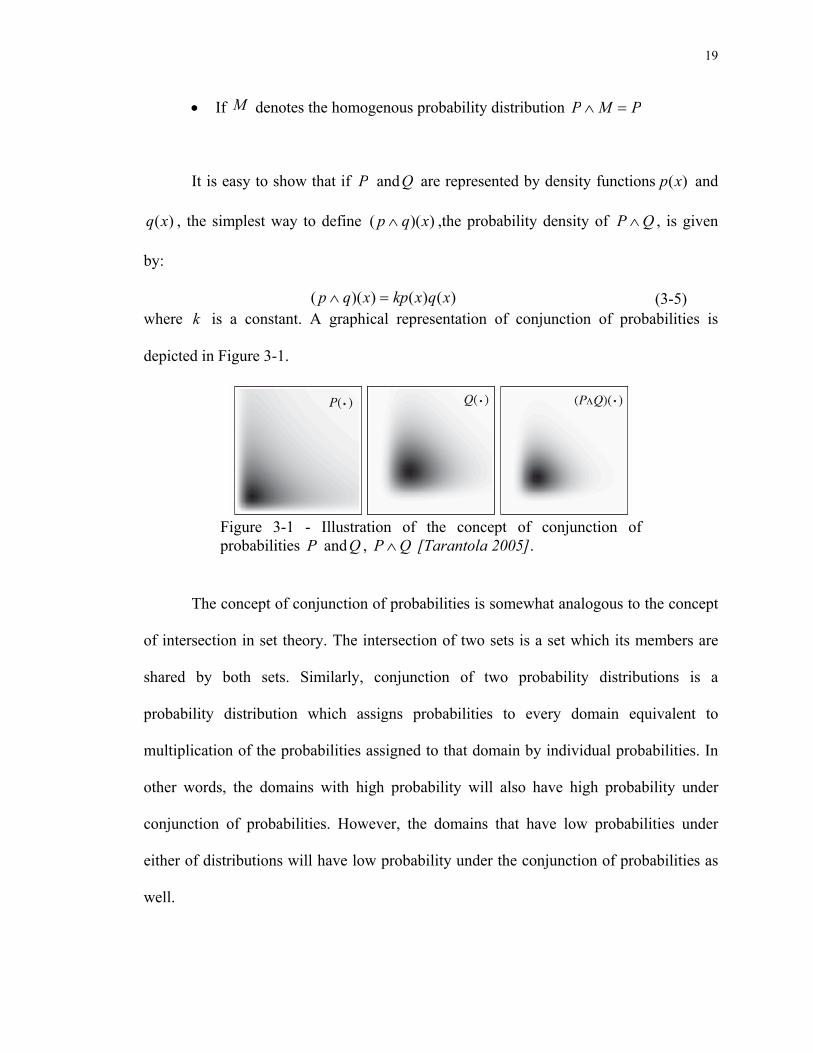
Consider two probability distributions P andQ . The conjunction of these

probabilities is a probability distribution denoted by QP ∧ which has the following

properties:

• PQQP ∧=∧ ;

• For any subset A , 0))(( =∧ AQP ; if and only if 0)( =AP and 0)( =AQ ;

19

• If M denotes the homogenous probability distribution PMP =∧

It is easy to show that if P andQ are represented by density functions )(xp and

)(xq , the simplest way to define ))(( xqp ∧ ,the probability density of QP ∧ , is given

by:

)()())(( xqxkpxqp =∧ (3-5) where k is a constant. A graphical representation of conjunction of probabilities is

depicted in Figure 3-1.

Figure 3-1 - Illustration of the concept of conjunction of probabilities P andQ , QP ∧ [Tarantola 2005].

The concept of conjunction of probabilities is somewhat analogous to the concept

of intersection in set theory. The intersection of two sets is a set which its members are

shared by both sets. Similarly, conjunction of two probability distributions is a

probability distribution which assigns probabilities to every domain equivalent to

multiplication of the probabilities assigned to that domain by individual probabilities. In

other words, the domains with high probability will also have high probability under

conjunction of probabilities. However, the domains that have low probabilities under

either of distributions will have low probability under the conjunction of probabilities as

well.

20

Marginal Probability

If the space is divided into two subspaces according to VU ×=χ , given the joint

probability density ),( vup , it is possible to derive marginal probability densities as:

∫=V

u vvupup δ),()( and ∫=U

v uvupvp δ),()( (3-6)

where u and v are points in subspace U and V respectively.

Independent Probabilities

If the u and v are independent parameters, their joint probability can be expressed as:

)()(),( vpupvup vu= (3-7)

Probabilistic Formulation of Inverse Problems Inverse problem is a mathematical problem where the objective is to obtain

information about a parameterized system (i.e. model) from observational data,

theoretical relationship between system parameters and data, and any available a priori

information. [Tarantola 2005, Parker, 1994, Menke 1984]. There are three major

components to any inverse problem:

• Parameterization of the physical system in terms of a set of model parameters

that from a given point of view completely describes the system.

• A set of physical laws called forward model that for a given set of model

parameters, makes prediction about the results of measurements.

• Use of the measurements of observable parameters to infer or invert the actual

values of the model parameters.

21

To be able to mathematically formulate the probabilistic solution of an inverse

problem, there are a few concepts that should be introduced.

Model Space and Data Space

For any given inverse problem, it is possible to select a set of model parameters

that will adequately describe the model (i.e. parameterization). The choice of these

parameters is not unique. However, once a particular parameterization of the system is

chosen, it is possible to introduce a space of values that describe possible values of model

parameters. This abstract space is termed the model space, and is denoted by M , which

represents all the conceivable models. Individual models, ,....},{ 21 mmm = are basically

points in the model space.

In an inverse problem, the values of parameters m are the main interest; however,

they are not directly measurable. The goal of inverse problem is to obtain information on

the values of m by making direct observation on another set of parameters denoted as

obsd . Similar to the concept of model space, it is possible to introduce an abstract idea of

data space D , which is the space of all conceivable observed responses. The actual

observed response is in fact a point in this space represented by ,...},{ 21 obsobsobs ddd = .

State of Information

In the probabilistic approach, any information about the problem, including the

solution of the problem, is expressed by probability distributions that are interpreted

22

using the concept of the state of information. The state of information is an intuitive

concept associated with the concept of probability. In addition to the statistical

interpretation of probability, a probability distribution can be also interpreted as a

subjective degree of knowledge of the true value of a given parameter. The subjective

interpretation of the probability theory is usually named Bayesian, in honor of British

mathematician Thomas Bayes (1763). The Bayesian interpretation of probability is a very

common concept in everyday life, which is used in many situations, such as in weather

forecast reports. For example, the forecast predicting a certain probability for having

precipitation presents the subjective knowledge of the meteorologist based on all the

available information. In civil engineering problems, the subjective knowledge about any

parameter prior to any measurement may also be represented by a probability

distribution. If there is no a priori information on the value of the parameter, this lack of

information can also be represented by a homogeneous probability distribution, where all

the possible models have the same probability. The other extreme situation is that when

the exact value of the parameter is known from a direct measurement. This precise

information can be also represented by a Dirac delta probability distribution. In general,

the spread of the probability distribution is an indication of how precise the knowledge

about the underlying parameter is; the narrower the spread of the distribution, the more

precise the prior information.

A Priori Information

In the probabilistic approach presented, the probability distribution representing

the state of information on the model parameters prior to the solution is denoted by

23

)(mMρ , and is termed the model a priori probability density function. Similarly, the a

priori information on the observed data prior to the solution can be expressed as data a

priori probability density function, which is denoted by )(dDρ . The a priori information

on model parameters (represented by )(mMρ ) is independent of a priori information on

the data (represented by )(dDρ ). This notion of independence can be used to define a

joint probability over the joint model and data space, ),( DM=χ , as a product of the two

marginal probability densities. This probability is denoted by:

)()(),( dmdm DM ρρρ = (3-8) where ),( dmρ is referred to as joint a priori probability density function and k is a

normalization constant. This probability can be graphically depicted as a “cloud of

probability” centered on the observed data and a priori model, as shown in Figure 3-2.

Figure 3-2 - Illustration of the probability densities

)(mMρ , )(dDρ , and ),( dmρ representing a priori information on model, data, and joint model and data spaces respectively [Tarantola 2005].

),( dmρ

24

Forward Model

The forward model is a set of physical laws that for a given set of model

parameters, Mm ∈ , predicts the value of observable parameters, Dd ∈ . The forward

model can be expressed as:

)(mgd = (3-9) where )(mg is the forward model operator. If the model predictions are exact and

without any uncertainty, a single response is predicted for a given model. However, the

forward model predictions are rarely exact and there are modeling approximations

involved. In the probabilistic approach, the effect of this approximation can be

represented by a probability density function, ),( dmθ . In this representation, for a given

model parameter, instead of a single value of d , a probability in the data space is

predicted representing the modeling uncertainties. This concept, as well as the probability

),( dmθ , referred to as forward model probability density function, is conceptually

depicted in Figure 2-3. It should be pointed out that evaluation of modeling uncertainties

is a complex task, and in many cases, there is only limited published research available.

For the applications presented in the chapters that follow, modeling uncertainties have

been assigned based on experience or limited analysis. Further research is required to

evaluate the modeling uncertainties for each application.

It is worthy to mention that for the formulation presented here, the forward model

is considered to be a general model and no simplifying assumptions, such as the linearity

assumption, are made. For example, if the forward model operator, (.)g , is a linear

operator (i.e. Gmd = , where G is a matrix), significant simplification of the inverse

problem theory can be obtained [Menke 1984]. However, to present a uniform approach

25

to both linear and non-linear inverse problems, for the treatment presented here a general

nonlinear operator is considered.

Figure 3-3 - (left) Forward model with negligible modelization uncertainties (right) and forward model with modeling uncertainties [Tarantola 2005].

General Probabilistic Solution of the Inverse Problem

In the probabilistic framework, the solution of an inverse problem is a probability

distribution combining the a priori information, ),( dmρ (i.e. experimental information),

with information obtained from the forward model, ),( dmθ (i.e. theoretical information).

Since the predictions of the forward model are assumed to be independent of a priori

information, the combination can be accomplished by conjunction operation [Tarantola,

2005], which can be visualized as the multiplication of two probabilities. The resulting

probability, denoted by ),( dmσ , is basically the solution of the problem, and it is termed

a posteriori probability, where its density function is represented by [Tarantola, 2005]:

),(),(),( dmdmkdm ρθσ = (3-10) where k is a normalization constant. The conjunction operation and the obtained

probability are depicted in Figure 3-4.

),( dmθ)(mgd =

26

Having defined the a posteriori probability, marginal probability densities on

model and data spaces are defined respectively as:

ddmmD

M δσσ ∫= ),()( and mdmdM

D δσσ ∫= ),()( (3-11)

where )(mMσ is model a posteriori probability density function, and )(dDσ is the data a

posteriori probability density function. The model a posteriori probability, as defined

above, is often the prime quantity of interest in the solution of an inverse problem.

Figure 3-4 - Representation of the general probabilistic solution of inverse problem as the conjunction of the a priori information, ),( dmρ and information obtained from forward model ),( dmθ . [Tarantola 2005].

Probabilistic Solution in the Case of Data and Forward Model with

Gaussian Uncertainties

Substituting Equation (3-10) into Equation (3-11), and using Equation (3-8), the

model a posteriori probability distribution (i.e. the problem solution in the model space)

can be evaluated as:

ddmdmkmD

DMM δθρρσ ∫= ),()()()( (3-12)

or

),( dmθ

),( dmρ ),( dmσ

27

)()()( mmkm MM λρσ = (3-13) where )(mλ is the likelihood function:

ddmdmD

D δθρλ ∫= ),()()( (3-14)

If it is assumed that the data uncertainties are represented by a Gaussian

probability, such as:

⎟⎠⎞

⎜⎝⎛ −−−= − )()(

21exp)( 1

obsdT

obsD ddCddkdρ (3-15)

where dC is the covariance matrix representing observational uncertainties, and that the

forward model uncertainties can be presented by:

⎟⎠⎞

⎜⎝⎛ −−−= − ))((())((

21exp),( 1 mgdCmgdkdm T

Tθ (3-16)

where TC is the covariance matrix representing forward model uncertainties. It can be

shown that the likelihood function can be represented by [Tarantola 2005]:

⎟⎠⎞

⎜⎝⎛ −+−−= −− ))(()(())((

21exp)( 11 mgdCCmgdkm obsdT

Tobsλ (3-17)

This result is important because it shows that, by the Gaussian assumption,

observational and modeling uncertainties simply combine by addition of their respective

covariances. It is worthy to mention that, by inspection of Equations (3-13) and (3-17), it

can be observed that, if there is no a priori information (i.e. )()( mmM µρ = ), the

maximum of the a posteriori probability occurs at the maximum of the likelihood

function. Additionally, the maximum of the likelihood function occurs when the observed

data fits best the model predictions in a weighted least square sense. If the covariance

matrices are multiplications of the identity matrix, it can also be shown that the maximum

of the likelihood function is the 2L norm best fit model to the observed data. This is the

28

same solution obtained in the deterministic approach. Therefore, it can be concluded that

the deterministic solution is a very special case of the probabilistic solution.

Appraisal of the Probabilistic Solution It has been stated and illustrated that the solution of the inverse problem, the a

posteriori probability distribution, is the conjunction of two probability distributions

representing experimental and theoretical information about the problem. Although the a

posteriori probability distribution contains all the information regarding the problem

solution, it is generally desirable to quantify this information. In other words, it is

desirable to appraise the obtained solution. Two important classes of quantities are

generally presented as quantifying measures of the a posteriori probability distribution:

(1) central estimators and estimators of dispersion, and (2) one and two dimensional

marginal probability densities.

Central Estimators and Estimators of Dispersion

The a posteriori mean model (or the expected value) is a central estimator, which

represents the most probable solution. It is calculated using following integral:

∫=⟩⟨M

M mmmm δσ )( (3-18)

where ⟩⟨. indicates the mean or expected value. It should be mentioned that depending on

the shape of probability distribution, the mean value may or may not coincide with the

maximum of probability density. The dispersion estimator associated with the mean is the

covariance matrix and is given by:

29

mmmmmmC MT

MM δσ )())(( ⟩⟨−⟩⟨−= ∫ (3-19)

Since the concept of mean and covariance is derived for unimodal probability

densities, for complex problems, where the posteriori probability density is complex and

may have several modes, one should be careful in interpretation of the mean and

covariance.

One and Two Dimensional Marginal Probability Densities

Another quantity of interest in presentation of probabilistic solution is the one

dimensional marginal probability density of variable im :

∫ ∫ ∏≠=

=Γ

ikk

kMi mmm1

)(...)( δσ (3-20)

where Γ indicates the marginal probability density. Joint marginal probability density of

two parameters can be defined in a similar manner:

∫ ∫ ∏≠≠=

=Γ

jkik

kkMji mmmm

1)(...),( δσ

(3-21)

Evaluation of the integrals presented in equations (3-18) thru (3-21) generally has

to be performed numerically. However, when the a priori and forward model probability

distributions are simple, it is possible to obtain closed form formulas that can be directly

used in evolution of estimator quantities and marginal probabilities [Menke 1984].

Summary The mathematical theory of inverse problems from a probabilistic view was

introduced in this chapter. The basic concepts and elements of the theory were presented

and the general solution of the inverse problem was defined as the a posteriori

30

probability, which combines the a priori information about the problem with the

information obtained by measuring some observable parameters (data) and theoretical

information gained from a forward model. The obtained general solution was then

formulated for the case where the data a priori and forward model probabilities are

Gaussian. Two important classes of quantities that are used for appraisal of the results,

namely, (1) central estimators and estimators of dispersion, and (2) one and two

dimensional marginal probability densities, were also introduced and defined.

References Kokmogorov, A.N., (1933), “Grundbegriffe der Wahrcheinlichkeitsrechnung “,

Springer, Berlin, Germany Menke, W. (1984), “Geophysical Data Analysis: Discrete Inverse Theory”, Academic

Press Inc. Orlando, FL. Mosegaard K. and Tarantola, A. (2002), “International Handbook of Earthquake and

Engineering Seismology – Chapter 16: Probabilistic Approach to Inverse Problems”, Academic Press, San Diego, CA.

Parker, R. L., (1994), “Geophysical Inverse Theory”, Princeton University Press, Princeton, NJ.

Tarantola, A. (2005), “Inverse Problem Theory”, SIAM, Philadelphia, PA. Tarantola , A, (2004), “Probability and Measurements”, Submitted to Cambridge

University Press for publication. Tarantola, A. and Valette, B. (1982), “Inverse Problem=Quest for Information”,

Journal of Geophysics, 50, p. 159-170.

31

4 Monte Carlo Evaluation of the Probabilistic Solution

Chance, too, which seems to rush along with slack reins, is bridled and governed by law.”

Boethius, Roman Philosopher, c.a. 480-525

Introduction Probabilistic formulation of inverse problems leads to the definition of the

solution as a probability distribution in the model space [Tarantola 2005]. This

probability distribution combines a priori information on the model parameters with new

information obtained by measuring some observable parameters (data) and theoretical

information gained from a forward model. For simple problems, it is possible to use the

derived mathematical equations directly and obtain an analytical solution of the inverse

problem. However, in general, due to the large number of the model parameters or the

complexity of the theory linking the data and the model parameters, it may not be

possible to describe the solution analytically. In such cases, one technique to evaluate the

solution is to randomly generate a large collection of models according to the a posteriori

probability distribution and analyze and display the models in such a way that

information about the underlying probability is conveyed. This approach can be

accomplished using a class of computational techniques referred to as Monte Carlo

methods.

32

This chapter introduces Monte Carlo techniques for evaluation of the probabilistic

inverse problem solution. To provide a context for practical applications and illustrate the

presented concepts and techniques, a simple inverse problem example, along with its

deterministic solution and analytical probabilistic solution, is initially introduced and is

used throughout the chapter. For complex problems where obtaining an analytical

solution is not feasible, a numerical technique using Monte Carlo Markov Chains

(MCMC) is introduced and its application is illustrated. To further reduce the

computational time in the solution of the complex problems, the MCMC technique is

integrated with the recently developed Neighborhood Algorithm (NA). NA and it

integration with MCMC are describes, and its application is illustrated using the

previously introduced example. It should be mentioned that there are other techniques

available for the evaluation of the probabilistic solution of inverse problems; however, a

through discussion of these techniques are beyond the scope of this research.

Illustrative Example A simple deflection based modulus determination experiment is presented below,

and it is used as the illustrative example throughout this chapter.

Deflection Based Modulus Determination Experiment: The objective of the experiment is to determine the elastic modulus of a cantilever beam from the measurement of the deflection of the beam. As depicted in Figure 4-1, the experiment is conducted by placing a known load P at a measured length L from the fixed end of the beam and measuring the deflection ∆ . In this inverse problem, modulus is the model parameter of interest and deflection is the observed data. The forward model predicting the deflection for any given modulus is simply obtained using mechanics of materials principles as:

33

EIPL3

=∆ (4-1)

where E is the modulus and I is the moment of inertia of the beam.

mL 5.0= , mb 05.0= , mh 01.0= , NP 100= , mobs 043.0=∆

Figure 4-1 - Deflection based modulus determination experiment.

Deterministic Solution In the deterministic approach, the objective is to find a set of model parameters

which minimizes the difference between the model prediction and the observed data (i.e.

obsdmg −)( ).

Deterministic Solution of the Modulus Determination Experiment: Based on the traditional deterministic solution, the modulus of the beam can be evaluated by:

obsobs I

PLEEIPL

∆=→∆−

33min (4-2)

Using the numerical values provided in Figure 4-1, GPaE 8.69= , which suggests that the material is probably an aluminum alloy. It should be mentioned that in the deterministic approach, no estimate of uncertainty is obtained.

34

Analytical Evaluation of the Probabilistic Solution If the a priori and forward model probability distributions are simple, it might be

possible to obtain a closed form analytical solution of the problem by direct application

of the presented relationships. This technique is illustrated below; however, in practice,

analytical solution can rarely be obtained, and only a numerical estimate of the solution

can be calculated.

Analytical Evaluation of the Probabilistic Solution of the Modulus Determination Experiment: To obtain a probabilistic solution, the a priori and forward model probability densities should be defined. Let’s assume a Gaussian a priori probability for observed data with the standard deviation ∆Σ ,

⎟⎟⎠

⎞⎜⎜⎝

⎛

Σ

∆−∆−

Σ⋅=∆

∆∆∆ 2

2)(21exp1

21)( obs

πρ , and an independent homogeneous a priori

probability density for modulus, E (representing no specific a priori information on the model parameter), kEE =)(ρ , where k is a constant.

As presented, in probabilistic approach, the uncertainties in forward model can also be incorporated in the solution. For many reasons, such as inherent simplifying assumptions in the derivation of the equation, uncertainties in evaluation of the model coefficients, etc, the given forward model, IEPL /3=∆ , can never be exact. Let’s assume that the leading cause of uncertainty in the forward model in this experiment is the uncertainty in the magnitude of the applied load. The forward model probability density can then be represented by the following probability density function:

⎟⎟

⎠

⎞

⎜⎜

⎝

⎛

Σ−∆

−Σ

⋅=∆ 23

23

3 )/()/(

21exp

/1

21),(

IELIEPL

IELE

ppπθ (4-3)

where pΣ is the standard deviation representing uncertainty in load P . This equation simply means that for a given modulus, E , rather than predicting a single deflection value, a Gaussian probability in the data space is predicted by the forward model, which incorporates the modeling uncertainties.

The solution of the inverse problem, the conjunction of probability densities, is then given by:

),()()(),(),(),( ∆∆=∆∆=∆ ∆ EEEEE E θρρθρσ (4-4)

or

35

⎟⎟

⎠

⎞

⎜⎜

⎝

⎛

Σ

∆−∆−

∆Σ∆−

−=∆∆

2

2

23

23 )(21

)/()/(

21exp),( obs

p ILIPLEkEσ (4-5)

where k is a constant. Probabilities )()(),( ∆=∆ ∆ρρρ EE E , ),( ∆Eθ , and ),( ∆Eσ are depicted in Figure 2-7.

Modulus (GPa)

Def

lect

ion

(m)

60 70 80 900.035

0.04

0.045

0.05

0.055

Modulus (GPa)60 70 80 90

Modulus (GPa)60 70 80 90

Figure 4-2 - Graphical representation of the probability densities ),( ∆Eρ , ),( ∆Eθ , and ),( ∆Eσ for the modulus determination experiment. It is assumed that Pap 1=Σ and

m001.0=Σ∆ . The maximum of the probability density ),( ∆Eσ , is located at GPaE 8.69= ,

which is the solution identified in deterministic approach. However, it can be observed that in addition to the reported value of the modulus, the solution depicted in Figure 4-2 conveys information about the uncertainties of the obtained results.

Appraisal of the Probabilistic Solution of the Modulus Evaluation Experiment:

The information contained in the solution probability density function can be quantified in terms of central and dispersion estimators, such as mean and variance. Often times, for complex problems, these quantities are the only results that are reported.

For this example, the a posteriori probability density on model space is simply:

∫∆ ∆

∆⎟⎟

⎠

⎞

⎜⎜

⎝

⎛

Σ

∆−∆−

∆Σ∆−

−= δσ 2

2

23

23 )(21

)/()/(

21exp)( obs

pE IL

IPLEkE (4-6)

This integral is numerically evaluated and the results are depicted in Figure 4-3.

),( ∆Eσ),( ∆Eθ),( ∆Eρ

36

60 65 70 75 80 85 90Modulus (GPa)

Pro

babi

lity

Figure 4-3 - Graphical representation of the probability density )(EEσ for the modulus determination experiment. It is assumed that Pap 1=Σ and m001.0=Σ∆ .

Using the numerically evaluated probability density, )(EEσ , mean and variance quantities can be evaluated as: GPaEE 8.69)( =σ and GPaCE 8.1= , where .

EC is the variance of )(EEσ .

Direct Sampling Evaluation of the Probabilistic Solution The ultimate objective of the direct sampling solution technique presented here is

to randomly generate a large representative collection of models according to the model a

posteriori probability distribution, )(mMσ , and analyze and display the sampled models

to derive information about the underlying a posteriori probability distribution. In

addition to the basic question of how to generate such samples, there are several other

issues, such as stability, convergence, and error estimates of the direct sampling approach

that need to be discussed and addressed. These issues are discussed and addressed in this

section.

37

Monte Carlo Sampling of Probability Distributions

It is only when the problem is very simple; the analytical techniques can be used

to characterize the solution. For more complex problems, one needs to perform an

extensive numerical exploration of the model space and characterize the probabilities for

each point in the model space. Except for the problems with a very small number of

dimensions, this exploration cannot be systematic. In such cases, well-designed random

(or pseudorandom) explorations can be used to solve the problem. These random

methods are generally referred to as Monte Carlo methods.

The term “Monte Carlo”, as it refers to computation calculations, was apparently

first used by the Enrico Fermi, Stanislaw Marcin Ulam, and John von Neumann as a code

name at Los Alamos laboratories for stochastic simulations in development of the atomic

bomb. The name Monte Carlo, an illusion to the famous casino in Monaco, refers to the

fact that these techniques use the law of random numbers in a similar way that is used in

casinos. Today, the Monte Carlo methods refer to any simulation that involves the use of

random numbers. Despite the wide spread use of these methods and numerous

descriptions of them in articles and books, it is not possible to find a complete and

comprehensive definition of Monte Carlo Methods. This is in part due to intuitive nature

of these techniques, which are used in a wide range of areas including physics, biology,

chemistry, and financial markets. In general, Monte Carlo methods provide approximate

solutions to a variety of mathematical problems by performing statistical random

sampling experiments. The methods apply to problems with no probabilistic nature as

well as to those with inherent probabilistic structure. While most applications of Monte

Carlo methods are performed on computers today, there are many applications using

38

coin-flipping, card-drawing, or needle-tossing experiments. However, advent of the

computers and their ever increasing computational capabilities, made it possible to

successfully apply Monte Carlo methods to more complex problems, including complex

inverse problems. A good review of historical development of Monte Carlo methods in

the context of inverse problems is given by Sambridge and Mosegaard [2002].

The fundamental idea behind Monte Carlo methods is that inference regarding the

characteristic of the parameters of interest can be gained by repeatedly drawing random

samples from the population of interest and observing the behavior of the parameters

over the samples. Such an approach is graphically illustrated in Figure 4-4 for a two

dimensional probability distribution.

Figure 4-4 - The collection randomly generated samples (right) of a probability distribution (left) allow inference of characteristics of underlying probability distribution [Tarantola 2005].

The fundamental question here is that given a probability distribution, defined

analytically or numerically, how random samples according to a desired probability

distribution can be generated? Markov chains provide the mathematical tools required for

generation of such samples.

39

Markov Chains

A Markov chain, named after the Russian mathematician Andrey Markov (1856-

1922), is a sequence of random numbers such that the next value or state of the sequence

depends only on the previous stage [Bhat and Miller, 2002]. This dependency is

mathematically described by transition kernel, )( 1 nn xx +ψ , which is the probability

distribution representing conditional probability of transition to 1+nx from nx . Thus a

sequence of random numbers 1x , 2x ,…, nx can be generated such that next state 1+nx is

distributed according to the transition kernel )( 1 nn xx +ψ . A realization of the sequence is

called a Markov chain. It is assumed here that transitional kernel does not change as the

sequence progresses, making the chain homogenous in time. It can be shown that given

certain conditions [Tierney, 1994] the chain will forgot its starting state and the

distribution of the random numbers will converge to a stationary or target distribution,

denoted as Ψ . In other words, as the sequence grows larger, the sample points nx will

become dependent samples of stationary distribution Ψ . The central question here is that

given )(xΨ as the desired stationary probability, how )(xψ should be constructed so that

Markov chain converges to )(xΨ . Metropolis sampler [Metropolis et al 1953] is one

technique for generating desired Markov chains with a given target distribution.

40

Metropolis Sampler

Metropolis sampler [Metropolis et al 1953] is a special case of Metropolis-

Hasting sampler [Hasting 1970]. The sampler is a set of rules that generates a Markov

chain with a given desired target probability, )(xΨ . To define the rules, consider a

Markov chain with a given state nx . To move to the next state, the Metropolis sampler

obtains a random candidate state, y (generated randomly most often from a uniform

distribution). If the value of )()( nxy Ψ>Ψ the candidate point is accepted and yxn =+1 .

If )()( nxy Ψ<Ψ , the candidate point is only accepted with a probability of

)(/)( nxy ΨΨ . Otherwise, the candidate point is rejected and nn xx =+1 . It can be shown

that the Markov chain generated in this manner will converge to )(xΨ . The Metropolis

sampler can be represented by the following generalized algorithm:

• Initialize the chain to 1x

• At n th state, randomly generate a candidate point y (usually derived from a

uniform distribution).

• If )()( nxy Ψ>Ψ accept the candidate and set yxn =+1 ;

• if )()( nxy Ψ<Ψ decide randomly to accept the transition with a probability

of )(/)( nxy ΨΨ , if the candidate is accepted set yxn =+1 ; otherwise set

nn xx =+1

• Set 1+= nn and repeat steps 2 through 5

The above rules are also referred to as the Metropolis acceptances rule.

41

Cascade Metropolis Sampler

The Markov chain in metropolis sampler only applies the Metropolis acceptance

rule once with )(xΨ target probability. Assume that the sampler is modified such that the

acceptance rule is applied in cascade each time with different target probabilities,

),(),(),( xxx Ψ ′′Ψ′Ψ … )(xnΨ It can be shown that the stationary probability of the chain

is simply obtained as multiplication of probabilities or )(...)()()( xxxx nΨ××Ψ ′′×Ψ′×Ψ .

The cascade application of Metropolis acceptance rule at each state nx can be

implemented by application of the following set of rules to generate the next state of the

chain:

• At n th state, randomly generate a candidate point y (usually derived from a

uniform distribution)

• If )()( nxy Ψ>Ψ then go to next step; if )()( nxy Ψ<Ψ decide randomly to

go to next step with a probability of )(/)( nxy ΨΨ ; If move to next step is

rejected then set nn xx =+1 , 1+= nn and go to step 1.

• If )()( nxy Ψ′>Ψ′ then go to next step; if )()( nxy Ψ′<Ψ′ decide randomly to

go to next step with a probability of )(/)( nxy Ψ′Ψ′ ; If move to next step is

rejected then set nn xx =+1 , 1+= nn and go to step 1.

• ….

• ….

42

• ….

• If )()( nnn xy Ψ>Ψ then accept the candidate and set yxn =+1 ; if

)()( nnn xy Ψ<Ψ decide randomly to accept the transition (i.e. yxn =+1 ) with

a probability of )(/)( nnn xy ΨΨ ; If the candidate is rejected then set

nn xx =+1 , 1+= nn and go to step 1.

Monte Carlo Markov Chain (MCMC) Sampling of the Solution of Inverse

Problems

As presented in the previous chapter, the probabilistic solution of the inverse

problem is the a posteriori probability, which can be presented as:

)()()( mLmm MM ρσ = (4-7)

where )(mMσ is the a posteriori probability density on the model space, )(mMρ is the a

priori probability density and )(mλ is the likelihood function. For the applications

considered in this research, it has been assumed that data and forward model uncertainties

are Gaussian. It has been shown in previous chapter that for Gaussian data and forward

model uncertainties, )(mλ can be represented by:

⎟⎠⎞

⎜⎝⎛ −+−−= −− ))(()(())((

21exp)( 11 mgdCCmgdkm dT

Tλ

(4-8)

where TC is the covariance matrix representing forward model uncertainties and dC is

the covariance matrix representing observational uncertainties. Equation 4-7 and 4-8

form the basis for the development of Monte Carlo sampling algorithm for the solution of

inverse problems.

43

The goal of the sampling algorithm is to sample the model space at a rate

proportional to model a posteriori probability ( )(mMσ ). To achieve this goal, using

Metropolis acceptance rule, the algorithm first generates samples of model space

according to the model a priori probability )(mMρ , then these samples are accepted or

rejected using cascade implementation of Metropolis acceptance rule based on their fit to

observed data defined by likelihood function )(mλ . In other words the sampling

algorithm is a cascade implementation of metropolis algorithm with probabilities )(mMρ

and )(mλ . This means that models that are consistent with a priori information as well as

observations are sampled most often whereas models that are incompatible with either a

priori information or observational data are sampled rarely. The algorithm described

above can be written as:

• Initialize the chain to model 1m

• At n th state, randomly generate a candidate model y (usually derived from a

uniform distribution).

• If )()( nMM my ρρ > then go to next step; if )()( nMM my ρρ < decide

randomly to go to next step with a probability of )(/)( nMM my ρρ ; If move to

next step is rejected then set nn mm =+1 , 1+= nn and go to step 2.

• If )()( nmy λλ > then accept the candidate and set yxn =+1 ; if )()( nmy λλ <

decide randomly to go to accept the transition (i.e. ymn =+1 ) with a

probability of )(/)( nmy λλ ; If the candidate is rejected then set nn mm =+1 ,

1+= nn and go to step 2.

44

The output of the algorithm consists of a collection of models that their statistical

properties are asymptotically proportional to a posteriori probability distribution in the

model space. More comprehensive description of this algorithm can be found in other

references [Mosengaard and Tarantola 1995].

Appraisal of Results

Central and Dispersion Estimators

Central and dispersion estimators for appraisal of inverse problem solution were

introduced in the previous chapter as integrals in the model space. In MCMC approach,

these integrals should be evaluated numerically. Since in MCMC applications the

integrand of these integrals is not explicitly defined and is only sampled at certain

random points, these evaluations are generally obtained using Monte Carlo integration

techniques over the model space. A brief description of Monte Carlo integration

techniques is presented below. Detail mathematical treatment of this subject can be found

in other references [Hammersley and Handscomb 1964].

Numerical Monte Carlo integration can be simply viewed as evaluation of

expected value of a function )(xf , denoted by )]([ xfE where x is a random variable

distributed according to )(xp .

∫= xxpxfxfE δ)()()]([ (4-9)

45

In general, x is considered to be in multidimensional space and )(xf and )(xp

are functions of x . If a sequence of random variables ix , distributed according to )(xp can

be generated, the integral in Equation (4-9) can be evaluated by:

fxfN

xfEN

ii =≈ ∑

=1)(1)]([

(4-10)

where sign indicates the average value and N is the number of random variables used

to evaluate the integral. This is simply evaluation of the expected value of )(xf . The law

of large numbers ensures that the Monte Carlo estimate converges to the true value of the

integral:

∑=

∞→=

N

iiN

xfN

xfE1

)(1lim)]([

(4-11)

The uncertainty in Monte Carlo integration is basically the standard deviation of

the estimate of )]([ xfE , which can be estimated by:

221 ffN

−=ε

(4-12)

where ∑=

=N

iixf

Nf

1

22 )(1 . It is notable that the error of Monte Carlo integration is

independent of dimension of the space and is simply dependent on the number of random

variables. This property of Monte Carlo integration makes it more efficient than

traditional quadrature techniques for evaluation of integrals in high dimensional spaces (5

or higher). This property is especially appealing for evaluation of integrals in inverse

problems, which often should be evaluated over a high dimensional space. Using this

technique, the integrals for estimation of central and dispersion estimators can be

evaluated as simple sums over sampled models.

46

Marginal Probability Densities

Evaluation of marginal probabilities is often carried out by constructing the

histogram or density estimates of the collected samples in MCMC. A histogram is the

simplest non-parametric density estimator and the one that is most frequently

encountered. To construct a histogram, the interval covered by the samples is divided into

equal sub-intervals, known as “bins”. Every time a sample value falls into a particular

bin, then a block of height one and width equal to the bin width is placed on top of

histogram at that particular bin. Once this operation is repeated for all the samples, the

obtained graph is called the histogram of the collected samples and is an estimate of the

underlying probability density. The major shortcoming of histogram is that it does not

provide a smooth evaluation of the probability density.

Histogram is a special form of general probability density estimators. In

constructing the histogram, once a sample falls in a bin, a unit box function centered at

the midpoint of the bin is added to the histogram. This is known as box kernel density

estimate. If instead of a box function, a smooth function is used, the final density estimate

would be smooth. In this research, a Gaussian density estimate with an optimal

bandwidth is used as the kernel density estimator function. The discussion of the details

of implementation of this technique and selection of an optimal bandwidth are beyond the

interest of this text and are presented in other references [Bowman and Azzalini, 1997]. In

this text only results of the probability estimates are presented.

To illustrate the ideas and methods presented, the example of deflection based

modulus evaluation experiment is considered again.

47

MCMC Evaluation of the Probabilistic Solution of the Modulus Determination Experiment: As presented previously, assuming a Gaussian distribution for modeling uncertainties, the forward model probability density for this example can be represented by:

⎟⎟

⎠

⎞

⎜⎜

⎝

⎛

Σ−∆

−Σ

⋅=∆ 23

23

3 )/()/(

21exp

/1

21),(

IELIEPL

IELE

ppπθ (4-13)

Furthermore, similar to the previous example, let’s assume a Gaussian a priori probability for observed data with the standard deviation of ∆Σ , which is represented

by ⎟⎟⎠

⎞⎜⎜⎝

⎛

Σ

∆−∆−

Σ⋅=∆

∆∆∆ 2

2)(21exp1

21)( obs

πρ . Finally, let’s consider a homogeneous a

priori probability density for model parameter, represented by kEE =)(ρ , which represents no specific a priori information on the model parameter, where k is a constant.

It has been shown in previous chapter that if data and forward model uncertainties are Gaussian, the likelihood function follows a Gaussian distribution, which its covariance is the sum of the covariances of the forward model and data a priori. Using this result, the likelihood function can be represented by:

⎟⎟⎟⎟

⎠

⎞

⎜⎜⎜⎜

⎝

⎛

Σ+Σ

−∆−=

∆232

23

)/(

)(

21exp)(

EILEI

PL

kEp

obsλ (4-14)

Using the numerical values provided previously, the MCMC solution of the problem can be obtained using the described direct sampling method. The histogram of 40000 sampled models and the corresponding probability density estimate are shown in Figure 4-5. The probability density estimate is obtained using a Gaussian kernel density estimate. Based on the results presented in Figure 4-5, it can be observed that the estimates of the a posteriori probability are very close to the one obtained by analytical techniques.

Appraisal of MCMC Solution of the Modulus Determination Experiment Using

Monte Carlo Integration: As presented in previous chapter, the mean and variance of the evaluated solution can be calculated by:

∫=⟩⟨E

E dEEEE )(σ

)())(( EEEEEdEC ET

EE σ⟩⟨−⟩⟨−= ∫

(4-15)

Using Monte Carlo integration, these integrals can be evaluated as simple sums over sampled a posteriori models:

∑=

=N

iiE

NE

1

1

2

1)(1 ∑

=

−=N

iiE EE

NC

(4-16)

Using the numerically evaluated probability density, )(EEσ , mean and variance quantities can be evaluated as: GPaEE 9.69)( =σ GPaCE 8.1= .

48

Convergence

One important issue in application of MCMC is to decide when to stop the chain

and evaluate the underlying probability based on the collected samples. This issue has

been explored both theoretically and empirically in literature. In fact, an active and

important subfield of MCMC research is focused on the investigation and development of

techniques to determine if a chain with finite number of samples have converged to

underlying probability distribution and can be used as a reliable basis for estimation of

the properties of the target distribution.

60 65 70 75 80 85 90Modulus (GPa)

Pro

babi

lity

60 65 70 75 80 85 90Modulus (GPa)

Pro

babi

lity

Figure 4-5 - MCMC solution of the deflection based modulus determination experiment. Histogram (top) and kernel density estimate (bottom) of the a posteriori probability density obtained from analysis of 40000 sampled models.

49

Theoretically, it has been shown [Tierney, 1994] that if a chain has three

conditions of irreducibility, aperiodicity, and invariance, then in limit, as the number of

the samples increases, the chain will converge to the target probability distribution. For a

Markov chain, irreducibility implies that it is possible to visit any state to from any other

given state in a finite number of steps. Aperiodicity means that the Markov chain does

not circle around in the states with a finite period and a finally, invariance refers to the

property of the chain that it will always converge to a unique distribution. It can be

shown that [Robert and Casella, 1999] the Markov chain generated by Metropolis

algorithm satisfies these conditions and therefore in the limit, as the number of samples

approaches to infinity, the chain will converge to underlying probability distribution.

Although this result proves the ultimate convergence of the chain, the primary

concern in implementation of MCMC methods is to decide if the chain has reasonably

converged in a finite number of steps. There has been very limited success in developing

theoretical techniques for determination of the convergence of a chain. In general, there is

no golden rule to determine the convergence. Available techniques aim at determination

of the convergence through empirical diagnostic methods [e.g. Gelman and Rubin, 1992,

Raftery and Lewis, 1992, Geweke, 1992, Roberts, 1992, Ritter and Tanner 1992, Zellner

and Min 1995]. Cowles and Carlin [1996] give a comprehensive review of the available

convergence diagnostics techniques. However, none of these techniques is general and it

is possible to find examples where each method fails. These techniques can be divided

into two general categories, techniques that rely on a single long chain to achieve

50

convergence and techniques that are based on comparison of several chains that are

generated simultaneously.

In the implementation used in this research, the convergence is assessed by

diagnostic technique proposed by Gelman and Rubin [1992]. In this technique, several

chains using the same probability are generated and compared. The lack of convergence

of chains is determined from comparison of the mean of each chain to other means and to

the mean obtained from mixing all chains together. If the calculated mean for each chain

is close to the mean from other chains and to the mean obtained from mixing all the

chains together, it can be assumed that chains have converged to the underlying

probability. This comparison is carried out by calculating a scale reduction factor, R , as

follows:

)11(ˆWB

mnm

nnR +

+−

=

(4-17)

where B is the variance between the means from m chains each with n numbers and W

is the average of the m within chain-chain variances. For slowly mixing chains, the value

of scale reduction factor, R , is greater than one and approaches to one as chains

converge. Gelman and Rubin suggest running chains until the scale reduction factor is

close to one and preferably below 1.2. Further details about this diagnostic technique and

other available techniques can be found in cited references.

Computational Limitations

As illustrated, MCMC technique is a general technique for solution of the inverse

problems and estimation of the a posteriori probabilities. However, to obtain the solution,

51

a large number of models should be sampled and the likelihood function for each of them

should be evaluated, which in turn requires the solution of the forward model. The

number of required samples is a function of the dimension of the model space and the

required precision in determination of the model parameters. However, as a general rule,

as the number of the model parameters or required precision increases, the required

number of samples increases as well. With the speed of modern computers, this might not

be a problem for inverse problems that have forward models with a short computational

time. However, for inverse problems where the computational time of the forward model

is substantial, the time required for generation and evaluation of a large number of

samples is prohibitive. In such cases, more sophisticated approaches should be used. The

approach presented in the next section is one of the possible approaches.

Direct Sampling Solution Using Approximation of the Likelihood Function

As illustrated, MCMC heavily relies on running the forward model and evaluating

the likelihood function. Consequently, it becomes inefficient once the required

computational time of forward model increases. One approach for the solution of the

inverse problems with computationally time consuming forward models (say more than

few seconds) is to construct an approximation of the likelihood function over the model

space with limited and targeted evaluations of forward model and use this approximation

for evaluation of MCMC solution of the inverse problems. Using this approach, the

number of forward model evolutions will be limited, which in turn reduces the required

solution time. In this approach, the solution of the inverse problem will be carried out in

two steps:

52

• Approximation stage: generation of approximate likelihood function and,

• MCMC stage: evolution of MCMC solution of the problem using generated

approximation.

The approximation stage is implemented here using the recently developed

Neighborhood Algorithm (NA) as the search and approximation tool [Sambridge, 1999].

A brief description of neighborhood algorithm is presented below. The MCMC has been

described in previous section.

Neighborhood Algorithm (NA)

Neighborhood algorithm is a recently developed search and approximation

algorithm. The objective of the algorithm is to find the optimum of an objective function

by preferentially sampling the good regions of the space, which have higher values of

function. This algorithm falls in the same class of global optimization methods such as

simulated annealing and genetic algorithm and can be directly applied for optimization

problems. However, rather than seeking a single optimal point, NA provides an

approximation of the objective function, which is preferentially sampled more at the good

regions of the space. The approximation constructed by NA (i.e. Neighborhood

approximation) is used here to approximate the likelihood function for the solution of

inverse problems using MCMC.

NA approximation of likelihood function has several important features that are

essential for obtaining MCMC solution of the inverse problem. The neighborhood

53

approximation is a global approximation to likelihood function through out the model

space. Additionally, neighborhood approximation is preferentially sampled more at the

regions of the model space with high value of the likelihood function resulting in a better

approximation in important regions of the model space. Given the right control

parameters, NA can locate the global optimum of the likelihood function and it will not

get trapped in a local optimum. This feature of the algorithm makes it especially useful in

the solution of highly nonlinear inverse problems, where the likelihood function might

have several peaks. Finally, the value of likelihood function using neighborhood

approximation can be efficiently calculated for every point in the model space.

NA is a global optimization algorithm. Consequently, an additional result of the

approximation stage is the identification of the maximum of the likelihood function (i.e.

maximum likelihood point). As shown in previous section, in certain situations, the

maximum of the likelihood function is the deterministic solution of the inverse problem.

So, in these situations, the probabilistic approach presented here also identifies the

deterministic solution as an intermediate step. In other words, for these problems, the

search stage can be thought of as deterministic solution of the problem and MCMC stage

as uncertainty evaluation stage.

Finally, it should be mentioned that the accuracy of the obtained MCMC solution

is directly related to the goodness of the approximation used for likelihood function,

which is a function of the degree to which important regions of the model space are

sampled. There is no general technique for evaluation of goodness of an approximation,

intuitively, the more exploration in model space, the better the approximation.

54

Implementation of NA

The basic premise of NA algorithm is to use previously evaluated samples to

construct an approximation to the objective function through out the model space and use

this approximation to guide generation of new models for which the forward model has to

be evaluated. In general, the objective function can be any function, however, for the

inverse problem solution presented here, the objective function is the likelihood function.

The generalized algorithm can be presented as follows:

• Construct the approximate likelihood function surface from the previous

Pn models for which the function value has been calculated (i.e. forward

model has been solves);

• Use this approximation to generate the next sn samples in the prospective

regions of the space and find the function value for them;

• Add sn to Pn and repeat all the steps again.

The two important missing detail of the above algorithm is how to construct the

approximate likelihood function surface and how to generate new samples. NA algorithm

uses a mathematical construct knows as Voronoi diagram [Voronoi, 1908] to construct

the approximate surface and generate new samples.

55

Voronoi Diagram

Voronoi diagram is a unique way of dividing the n-dimensional space into

n regions called cells. Each cell is simply the nearest neighborhood region about one of

the previous samples as measured by a particular distance measure (most often 2L norm).

A set of two-dimensional Voronoi cells about 30 random samples is presented in Figure

4-6.

Figure 4-6 - Typical Voronoi Diagram in two dimensions.

Voronoi diagram provides a basis for construction of an approximation to

objective function. In NA, the approximate value of the likelihood function within each

Voronoi cell is assumed to be constant and equal to the value of the likelihood function

evaluated for the point inside the cell. Once this approximation (i.e. neighborhood

approximation) is constructed, NA uses this surface to guide the selection of the new

samples. Using the concept of Voronoi cells, NA algorithm can be re-written as follows:

• Generate initial sn samples in model space;

56

• Solve the forward model for the most recent samples and choose rn models

with highest objective function values,

• Generate sn new models by drawing random samples in the Voronoi cells of

each rn models (i.e. sn / rn samples in each cell).

• Go to step 2.

This algorithm preferentially draws samples in the regions of the model space

with high function value. The algorithm has only two control parameter sn and rn which

can be reduced to only one by setting rs nn = . At each step during the progress of

algorithm, the maximum of the function can be easily identified among the set of

sampled points and the approximate function can be created using neighborhood

approximation.

Stop Criteria

An important issue in implementation of NA is to determine when to stop the

algorithm. Since the objective of the algorithm is to optimize the objective function by

preferentially sampling the good regions of the space, the stop criteria should be directly

related to how precise the optimum point is located. Consider the following two stop

criteria, which both should be satisfied to stop the algorithm:

• The cell corresponding to the identified optimum has not changed for last sn

sampled points

57

• The distance (in 2L sense) between identified optimum and last sn sampled

points is less that ε , the required precision.

These two criteria ensure that the region containing the optimum point is sampled

adequately and additional sampling is not likely to change the location and precision of

the identified optimum. These criteria were used as the stop criteria for the algorithm.

Monte Carlo Solution Using Neighborhood Approximation

Once the approximation to likelihood function is constructed, it can be used to

obtain MCMC solution of inverse problem. If this approximation is dented as )(mNAλ ,

the solution can be represented as:

)()()( mmm NAMM

NA λρσ = (4-18) where )(mNA

Mσ is the a posteriori probability density obtained by using neighborhood

approximation, and )(mMρ is the model a priori probability density. MCMC techniques

as described above can be directly applied to obtain the solution )(mNAMσ and determine

estimator quantities and marginal probabilities.

To illustrate the application of the direct sampling using NA approximation of the

likelihood function, the modulus determination experiment is considered again. However,

to further demonstrate the advantage of the probabilistic approach in comparison to the

deterministic approach, the experiment design is slightly modified.

Deflection Based Modulus and Load Determination Experiment: In previous examples, the beam modulus was the only model parameter that had to be determined

58

from the solution of the inverse problem. For this example, it is assumed that in addition to the modulus, the exact magnitude of the load is also unknown and only an approximate magnitude is known. Therefore, in this example, there are two model parameters load, P , and modulus, E , which should be determined using one measured data value. It should be mentioned that in this case there is an infinite number of deterministic solutions. However, there is always a unique probabilistic solution to the problem. In reality, the a priori information on the model parameters, such as judgment on the type of material or simply an estimate of the load, might be enough to limit the solution to a set of probable solutions. However, there is no structured procedure in the deterministic approach to include such information in the solution process. However, they can be easily included in the probabilistic approach.

Assume that there is no specific a priori information on modulus, i.e. it is represented by a homogenous a priori probability. However, based on the available information, a Gaussian a priori probability for load, P , can be formed, which conveys the expected value of the load. These probabilities are represented by:

⎟⎟

⎠

⎞

⎜⎜

⎝

⎛

Σ

−−

Σ⋅= 2

2)(21exp1

21)(

Ppri

pri

PpriPpri

PPP

πρ

kEEE == )()( µρ

(4-19)

where priP and PpriΣ are the mean and variance of the a priori distribution. For this example, since the uncertainty of the load is considered as an a priori information, the likelihood function can be simplified as:

⎟⎟⎟⎟

⎠

⎞

⎜⎜⎜⎜

⎝

⎛

Σ

−∆−=

∆2

23

)(

21exp),( EI

PL

kPEobs

λ

(4-20)

Having defined the elements of the problem, the MCMC solution of the problem using NA is presented below. The solution consists of two stages, approximation stage and MCMC stage.

Approximation Stage: The neighborhood approximation of the likelihood function, obtained using neighborhood algorithm, is presented in Figure 4-7. Since the likelihood function in this example is simple, for comparison purposes, exact plot of the function is also presented. It should be remembered that this exact plot is generally not available. By inspection of this figure, it can be observed that the neighborhood approximation is relatively coarse where the value of the function is low and it becomes dense near the regions of the function with high values. It should be also noted that the likelihood function in this case is a function which has infinite number of maximum points. This type of behavior is not easy to approximate. However, it can be observed that the neighborhood approximation has reasonably captured the behavior of the function.

MCMC Stage: The two dimensional a posteriori histograms of 10000 sampled models obtained using the neighborhood approximation of the likelihood function are presented in Figure 4-8. For comparison purposes, the analytical solution is also presented in this figure. Histogram and kernel density estimates of one dimensional posteriori marginal probabilities for each parameter are also presented in Figure 4-9.

59

Using the numerically evaluated probability density, mean and variance quantities for the modulus and load are presented below:

GPaEE 6.72)( =σ , GPaCE 66.10= GPapp 4.100)( =σ

, GPaCP 18.10= It can be observed that the approximate solution has captured the essential

features of the exact analytical solution.

Modulus (GPa)

Load

(Pa)

40 50 60 70 80 90 10040

60

80

100

120

140

Modulus (GPa)

Load

(N)

40 50 60 70 80 90 10040

60

80

100

120

140

Figure 4-7 - Exact plot (top) and neighborhood approximation (bottom) of the likelihood function with 1000 models. Sampled models, as well as corresponding Voronoi diagram are also shown ( m001.0=Σ∆ ).

60

Matlab® Application Program To implement the outlined probabilistic approach, a user friendly Matlab® based

application is prepared to evaluate the probabilistic solution with NA approximation. The

application, which uses Matlab® scripts as inputs, is designed as a general purpose

inversion tool for the solution of different inverse problems and is used for applications in

the following chapters. A snapshot of the input window of this application is presented in

Figure 4-10.

Modulus (GPa)

Load

(N)

40 50 60 70 80 90 10040

60

80

100

120

140

Modulus (GPa)

Load

(N)

50 60 70 80 90

60

80

100

120

140

Figure 4-8 - Exact plot of ),( PEσ (top) and MCMC solution using neighborhood approximation (bottom) of the modulus determination experiment

61

40 50 60 70 80 90 100Modulus (GPa)

Pro

babi

lity

40 60 80 100 120 140Load (N)

Pro

babi

lity

20 40 60 80 100 120Modulus (GPa)

Pro

babi

lity

40 60 80 100 120 140Load (N)

Pro

babi

lity

Figure 4-9 Histogram of 10000 samples of the one dimensional marginal a posteriori probabilities of (a) modulus and (b) load, and their corresponding kernel density estimates (c and d)

Summary In this chapter, a number of techniques for quantitative evaluation of the

probabilistic solution were presented. The techniques for direct analytical evaluation and

numerical approximation of the probabilistic solution using Monte Carlo Markov Chains

(MCMC), with and without Neighborhood Algorithm (NA) approximation, were

introduced and explained. To demonstrate the advantages of the presented approach and

to illustrate the concepts and techniques in more practical terms, a very simple modulus

62

determination experiment was presented. It has been shown that the major advantage of

the probabilistic approach to inverse problem is its capability to evaluate the uncertainty

measures for the solution. Additionally, it has been shown that the a priori information

about the model parameters can be readily incorporated in the probabilistic solution

process.

Figure 4-10 Snapshot of the input window of ProbInvert, the developed probabilistic inversion application.

63

References Bhat, U. N. and Miller, G. K. (2002), “Elements of Applies Stochastic Processes”,

John Willey & Sons Inc., Hoboken, NJ. Bowman, A.W. and Azzalini A. (1997), “Applies Smoothing Techniques for Data

Analysis: The Kernel Approach with S-PLUS Illustration”, Claredon Press, UK. Cowles, K. and Carlin P. (1996), “Markov Chain Monte Carlo Convergence

Diagnostics: A Comprehensive Review”, Journal of American Statistical Association, 91 (434), 883-904.

Gelman, A. and Rubin, D.B. (1992), “Inference from Iterative Simulation Using Multiple Sequences”, Statistical Science, 7, 457-511.

Geweke, J. (1992), “Evaluation of the Accuracy of Sampling Based Approaches to Calculation of Posterior Moments”, in Bayesian Statistics 4, eds. M. Bernardo, J. Berger, A. P. Dawid, and A. F. M. Smith, Oxford University Press, Oxford, UK.

Hammersley, J. M. and Handscomb, D. C. (1964), “Monte Carlo Methods”, Methuen and Co. Ltd, London, UK.

Hastings W. K. (1970), “Monte Carlo sampling methods using Markov chains and their applications”, Biometrika, 57:97-109.

Metropolis, N., A. W. Rosenbluth, M. N. Rosenbluth, A. H. Teller, and E. Teller. (1953), “Equation of state calculations by last computing machines”, J. Chem. Phys. 21:1087-1092.

Mosegaard K. and Tarantola, A. (1995), “Monte Carlo Sampling of Solution to Inverse Problems”, Journal of Geophysical Research, Vol.100, No. B7, p 12,431-12,447.

Raftery, A. E. and Lewis, S. (1992), “How Many Iterations in Gibbs Sample?”, in Bayesian Statistics 4, eds. M. Bernardo, J. Berger, A. P. Dawid, and A. F. M. Smith, Oxford University Press, Oxford, UK.

Robert, C. P., and Casella, G. (1999), “Monte Carlo statistical methods”, Springer-Verlag, New York, NY.

Roberts, G. O. (1992), “Convergence Diagnostics of Gibbs Sampler”, in Bayesian Statistics 4, eds. M. Bernardo, J. Berger, A. P. Dawid, and A. F. M. Smith, Oxford University Press, Oxford, UK.

Ritter, C. and Tanner, M. A. (1992), “Facilitating the Gibbs Sampler: The Gibbs Stopper and the Griddy-Gibbs Sampler”, Journal of American Statistical Association, 87, 861-868.

Sambridge, M. (1999), “Geophysical Inversion with Neighborhood Algorithm – II. Appraising the Ensemble”, Geophysical Journal International, 138, 727-746.

Sambridge, M. (1999), “Geophysical Inversion with Neighborhood Algorithm – I. Searching the Parameter Space”, Geophysical Journal International, 138, 479-494.

Sambridge, M. and Mosegaard K. (2002), “Monte Carlo Methods in Geophysical Inverse Problems”, Reviews of Geophysics, 40,3.

Tarantola, A. (2005), “Inverse Problem Theory”, SIAM, Philadelphia, PA. Tanner, M. (1996), “Tools for Statistical Inference”, Springer-Verlag, New York,

NY. Tierney, L. (1994),” Markov Chains for Exploring Posterior Distributions”, Annals of

Statistics, 22, 1701-1728.

64

Zellner, A. and Min, C. K. (1995), “Gibbs Sampler Convergence Criteria”, Journal of American Statistical Association, 90, 921-927.

65

5 Application One: Falling Weight Deflectometer Backcalculation

Introduction Falling weight deflectometer test, commonly referred to as FWD test, is the most

widely accepted, used, and studied technique for in-situ non-destructive evaluation of

pavements. The objective of the test is to excite and measure the pavement response

under the load levels equivalent to those applied on pavements by truck traffic. The

measured pavement response is then analyzed or backcalculated to infer elastic moduli of

pavement layers. FWD test is a very important tool for evaluation, design, and

maintenance of transportation infrastructure. The test is routinely used by pavement

engineers to backcalculate and estimate the in-situ pavement layer moduli, design

overlays, estimate remaining life of pavements, evaluate load transfer capability, and

perform network level monitoring.

In this chapter the probabilistic backcalculation of FWD test results is introduced

as the first example of the application of the probabilistic solution of inverse problems in

civil engineering. Introduction of limited probabilistic concepts in FWD backcalculation

has been previously suggested by others [e.g. Zaghloul et al, 2004]. However, to the

author’s knowledge, the presented approach in this chapter is the most comprehensive

and structured treatment of probabilistic backcalculation of FWD test results. Following

66

the introduction, a review of the FWD test procedure and current backcalculation

techniques are provided. The backcalculation problem is then formulated from a

probabilistic point of view and the results of the probabilistic backcalculation of synthetic

test data are presented. To compare different methods of FWD backcalculation, such as

static vs. dynamic and deflection bowl vs. time history backcalculation, the same set of

synthetic test data are backcalculated using different methods and the results are

compared. To illustrate the applicability of the developed backcalculation approach to

actual field data, a set of experimental FWD test results are backcalculated using the

probabilistic approach and the results are presented. The chapter concludes with a

discussion of the importance of considering the frequency dependence of layer moduli on

backcalculation results. This effect is evaluated using a spectral element model, which

simulates the pavement response in the frequency domain. The developed spectral

element model is used to backcalculate the same set of synthetic test results used

previously. The results of the backcalculation are presented and compared to other

results.

Background

Review of FWD Test Procedure

FWD test is conducted by dropping a weight on a guided system from a series of

predetermined heights and monitoring the ensuing pavement response. The test procedure

with FWD is documented in ASTM 4694-96 [ASTM, 1996] and ASTM D4695-03

[ASTM, 2003]. Schematics of the test setup and one of the trailers developed

commercially for its implementation are depicted in Figure 5-1.

67

During each drop, an approximately a half sine transient impulse force is applied

to the pavement. Currently available FWD trailers can apply loads ranging from 13600 to

over 227000 N (3000 to over 50000 lb). The equipment has a relatively low preload so its

influence on the pavement response is relatively negligible. The falling weight is

generally dropped on a composite loading plate with a 0.30 m (12 inch) diameter. The

composite plate generally consists of a steel plate, a PVC plate, and a rubber pad placed

on the lower surface of the plate, which rests on the pavement. The function of the

composite plate is to distribute the impact force, transferred to the plate via rubber buffers

attached to the bottom of the weight, rather uniformly over the pavement surface.

However, numerical studies have shown that for flexible pavements with a low paving

layer modulus, the interaction between the pavement and the loading plate during the test

might be significant enough to influence the stress distribution over the pavement surface

and produce a non uniform distribution [Boddapati and Nazarian 1994].

The FWD loading cycle is about 30 to 40 msec long. The transferred load to

pavement and pavement response during the test is generally monitored for 60 msec by

transducers resting at different radial offsets from the impact location. A typical loading

history and corresponding deflection time history records measured during FWD test are

depicted in Figure 5-2. The transferred load is commonly recorded by a load cell and

pavement response is monitored by geophones. It is common practice to measure the

pavement response at offset distances recommended by Federal Highway Administration

(FHWA) for Long Term Pavement Performance (LTPP) study. These offsets are 0, 0.20,

0.30, 0.45, 0.60, 0.90, 1.20 and 1.50 m (0, 8, 12, 18, 24, 36, 48 and 60 inch respectively).

During an FWD test, after dropping the weight and completion of initial loading and

68

unloading cycle, the weight loses contact with the plate for a time period after which the

contact takes place again. Previous studies have indicated that for the most conservative

lower drop heights the time interval between two contacts is about 180 msec.

Consequently, considering the duration of initial FWD impulse, the initial pavement

response during the FWD test can be considered independent of the subsequent rebounds

and impacts of the weight [Sebaaly, Davies and Mamlouk, 1985].

Figure 5-1 - Schematics of FWD test setup (top) and Dynatest® model 8000 FWD trailer (bottom).

69

0 10 20 30 40 50 60-10

0

10

20

30

40

50

60

70

Time (msec)

Forc

e (K

N)

0 10 20 30 40 50 60-0.12

-0.1

-0.08

-0.06

-0.04

-0.02

0

0.02

time (msec)

Def

lect

ion

(mm

)

r=0 mmr=203 mmr=305 mmr=457 mmr=610 mmr=914 mmr=1219 mmr=1524 mm

Figure 5-2 - Typical measured loading history (top) and pavement response during FWD test at different offsets (bottom).

Review of Current FWD Backcalculation Procedures

Over the past few decades, there has been a considerable number of publications

addressing different aspects of interpretation and backcalculation of FWD test results

with many of the important findings presented in several volumes of American Society

for Testing and Material (ASTM) special technical publications [Bush and Baladi, 1989,

Von Quintus, Bush, and Baladi 1994, Tayabji and Lukanen, 2000]. The review of

currently available backcalculation procedures indicates that the available procedures use

70

a deterministic approach to the solution of the problem. These procedures can be divided

into several categories based on the degree of complexity of the forward model used

[Uzan 1994], such as:

• Static linear elastic procedures,

• Static nonlinear elastic procedures,

• Dynamic linear procedures using either time or frequency domain fitting, and

• Dynamic nonlinear procedures.

In static linear elastic procedures, the theoretical static response of an elastic

pavement model under the maximum applied load is matched to the maximum measured

deflection of the pavement at each transducer location. The maximum deflection of the

pavement at each receiver is collectively referred to as the deflection bowl. Due to

simplicity and speed of calculation, static linear backcalculation procedures are widely

used in the current engineering practice. There are several programs available that

implement this approach, such as MODCOMP [Irwin, 1993], Modulus [Michalak and

Scullion, 1995] and ELMOD [ELMOD, 2001].

In static non-linear backcalculation schemes, a nonlinear static model is used to

generate a theoretical pavement response that matches the observed deflection bowl. The

main premise of the static non-linear backcalculation scheme is that by considering the

nonlinear effects, a more realistic theoretical model of pavement is used, which

consequently provides a better backcalculated estimates of pavement material properties.

The non-linear forward model is generally developed and analyzed using Finite Element

71

(FE) programs. There have been also attempts to include nonlinear effects in linear static

analysis by using empirically or theoretically generated relationships. Static non-linear

models in theory can provide a better representation of pavement response, however,

since the static model does not consider the dynamic nature of the FWD test, the validity

and accuracy of the static non-linear backcalculation approach are questionable.

The FWD loading cycle can not be in any sense considered as a static loading, as

is assumed in static procedures. There have been several studies against using static

pavement models in the FWD backcalculation [Mamlouk 1987, Uzan 1994, Alkhoury et

al 2001]. However, there is a general notion that in absence of a shallow bedrock (<3m)

and stiff and thick surface layer, the results of static linear backcalculation are reliable

[Uzan 1994].

In the dynamic linear analysis the theoretical dynamic pavement response is

matched to the observed deflection bowl or time histories. The calculation of forward

model can be implemented either in the time domain using either finite element or finite

difference techniques [Loizos and Scarpas 2005] or in the frequency domain using

analytical techniques, such as the transfer matrix approach suggested by Thomson [1950]

and Haskell [1953], which was further developed by Kausel and Roesset [1981], or the

spectral element technique [Doyle, 1997]. The studies by Uzan [1994] and Alkhoury et

al. [2001 a,b] are examples of successful application of dynamic linear forward model in

the FWD backcalculation. Although dynamic modeling of a pavement for generation of

the theoretical response is fundamentally a more appropriate approach to FWD

backcalculation [Zaghloul et al. 1994], due to a restrictive computational cost, its

application is currently very limited. However, with ever increasing computational power

72

available to practitioners, it is expected that dynamic modeling for backcalculation will

be used more extensively in future.

As partially outlined above, there have been a few decades of effort by engineers

and researchers to improve the FWD backcalculation procedures. Despite the extensive

research on FWD backcalculation and significant advances in this area, the current

backcalculation procedures still use a deterministic approach, which lacks uncertainty

measures. Adoption of the probabilistic approach in FWD backcalculation would

improve the current backcalculation procedures by evaluation of uncertainties in the

analysis, especially in the following areas:

• Evaluation of uncertainties in backcalculation results due to uncertainties in

the layer thickness input: Probably the most restrictive aspect of the FWD test

is that it requires knowledge of the pavement layer thickness as an input to

backcalculation routines. Such information is rarely available for every

location and should be estimated from other data. The uncertainty in the

thickness estimates used in the backcalculation translates to uncertainty in

obtained results, which is not possible to evaluate with current backcalculation

procedures. In the probabilistic approach, such estimates can be obtained.

• Evaluation of uncertainties due to selection of backcalculation variables: The

backcalculation results may vary depending on how the pavement model is

developed and the model parameters, such as the number and thickness of

pavement layers, are selected. Inappropriate selection of the model parameters

may produce poor backcalculation results. For example, it is generally

73

accepted that when a thin paving layer (<80mm) exists, its modulus can not be

reliably backcalculated. In the current backcalculation procedures, if such a

layer is selected as one of the parameters, there is no measure that determines

the uncertainty of the obtained results. In the probabilistic approach,

uncertainty measures are obtained as a part of the solution.

• Evaluation of uncertainties due to uncertainty in evaluation of the depth to

shallow bedrock: The presence of a shallow bedrock affects the results of

FWD test. Current practice relies on the analyst to detect presence of the

bedrock from the recorded data and estimate the depth to the bedrock from a

separate analysis and include it in the backcalculation analysis [Roesset et al.

1995]. The inaccuracy in determination of the depth to bedrock affects the

analysis results and increases uncertainties. In the probabilistic approach,

these uncertainties can be quantified.

Furthermore, since the probabilistic approach presented here uses a global search

algorithm, the obtained results are repeatable, which is not generally the case for some of

the available backcalculation procedures [Uzan 1994]. Using the probabilistic approach,

also allows exploration of the possibility of simultaneous backcalculation of the layer

moduli, depth to bedrock, and layer thicknesses as a part of the backcalculation analysis

along with associated uncertainty measures.

74

Probabilistic Formulation of FWD Backcalculation Using the notion of generalized measurement presented in the previous chapters,

the FWD test and the associated backcalculation can be considered as a generalized

measurement of pavement layer properties using surface deflection measurements. The

notion of a generalized measurement combined with tools developed in the previous

chapters will be used here to backcalculate the pavement layer properties and obtain

uncertainty measures.

As presented in the review section, there are different approaches to the modeling

of the pavement response in backcalculation of FWD test results, such as static or

dynamic modeling. Similar to the deterministic formulation of FWD backcalculation, the

probabilistic approach can also be formulated using different types of forward models. In

this study, two general types of forward models are considered and probabilistic

backcalculation is formulated using each of those:

• Probabilistic formulation using static linear elastic forward model: Although

the nature of the FWD test is obviously dynamic, due to their simplicity and

computational savings, historically, static forward models have been used to

model FWD test in backcalculation procedures. Since the static

backcalculation routines are still very popular with practicing engineers, this

class of backcalculation procedures is reformulated probabilistically to

investigate the uncertainties in the obtained results from this approach.

• Probabilistic formulation using dynamic linear elastic forward model:

Intuitively, the dynamic backcalculation approach should provide a more

realistic estimate of the pavement layer properties. The deterministic dynamic

75

backcalculation routines based on complete time history records of the

pavement deflection have been previously proposed for FWD backcalculation

[e.g. Alkhoury, 2001]. The probabilistic approach, in addition to more realistic

modeling of the pavement response, provides the required tools to investigate

the information carried by recorded data to backcalculate the layer moduli,

obtain uncertainty measures, and consider the possibility of directly

backcalculating other pavement properties, such as the depth to bedrock or

even pavement layer thicknesses.

The probabilistic formulation of a FWD backcalculation in terms of the a priori

information and the forward model operator is presented below and its application is

illustrated by backcalculation of synthetic and experimental FWD test data.

Model a Priori Information

In the probabilistic formulation, the model a priori information, represented by

probability density )(mMρ , presents the knowledge about the value of the model

parameters prior to the solution of the problem. For pavement layer properties, most

often, there is no information available other than possible limits of the value of the

parameters. The information about the limits of the value of the parameter of interest is

presented by a homogenous probability density. Since this type of a priori information is

the most common type encountered in practice, it is the only a priori information

considered here. Homogenous a priori probability densities considered for all pavement

layer properties in this chapter can be presented by:

76

⎪⎩

⎪⎨

⎧−=

0

1)( minmax mmmMρ

otherwise

mmm minmax <<

(5-1)

where maxm and minm are respectively the maximum and minimum limits of the value of

the parameter of interest, m . The choice of limits of m generally depends on the

problem and the experience and judgment of the analyst. However, when in doubt, a

larger interval should be selected.

Data a Priori Information

Data a priori information, represented by probability )(dDρ , expresses the

uncertainties in the measurement of the observed parameters, which for a FWD test are

simply deflections at transducer locations.

The uncertainties in deflection measurement can be divided into two categories

according to guidelines of United Stated National Institute of Standards and Technology

(NIST): uncertainties of “Type A” and “Type B” [Taylor and Kuyatt, 1994]. The

uncertainties in deflection measurement of the transducers are usually evaluated as a

“Type A” uncertainty by the transducer manufacturer. For example, for Dynatest 8081

FWD/HWD system, these uncertainties are quantified in the owner’s manual as, “The

deflections are measured with an absolute accuracy of better than 2%±2 microns, and

with typical, relative accuracy of 1%±1. The resolution of the equipment (in terms of

deflection) is one micron” [Dynatest, 1995]. However, in addition to uncertainties

associated with instrument measurements, there are generally other uncertainties in FWD

measurements that should be considered, such as the uncertainties in positioning and

appropriate contact of the transducers, uncertainties in instrument readings due to

77

vibrations sources other than the FWD impact, and uncertainties due to presence of

surface cracks. Ideally, each component of uncertainty should be evaluated statistically

and combined with other components to obtain the standard combined uncertainty.

However, in absence of such an evaluation, a reasonable estimate of uncertainty can be

obtained from repeatability studies reported in literature. The repeatability of FWD

measurements for several commercially available trailers is presented in Figure 5-3.

Based on these studies data a priori probability distribution, )(dDρ , will be considered to

be a Gaussian distribution with a mean equal to the observed value and a coefficient of

variation of two percent.

It should be mentioned that in a repeatability study each reading of the device is

compared to previous readings of the same device, not to the actual value of the

measurand. So, there is a difference between the result of repeatability studies and

uncertainties. However, in absence of any measure of uncertainty, the repeatability results

are used here as a rough estimate of the uncertainty in FWD measurements. Obviously, a

more thorough evaluation of the uncertainty of FWD measurements in the probabilistic

context would be required for more accurate estimates.

78

Figure 5-3 - Coefficient of variation of deflection from short term repeatability experiments [Benson, Nazarian and Harrison, 1994]. D1 thru D6 indicates different deflection sensors.

79

Forward Model

There are several approaches towards the modeling of the FWD test. The choice

of the model depends on many factors, such as the type of analysis, required degree of

complexity, computational requirements, and availability of resources. For this research a

finite element model was selected as the forward model. In finite element analysis, the

pavement response is generally calculated in the time domain. The main benefit of the

finite element model is its generality and the ease of modeling different geometries,

boundary conditions, and material models using commercially available and verified

codes. Finite element analysis can also be used to obtain the static response of the system

for a comparison to conventional backcalculation methods. The main disadvantage of the

finite element analysis is its computational cost.

The finite element forward model for this study was developed using ABAQUS®

program [ABAQUS, 2005]. The developed finite element mesh is presented in Figure 5-4.

The same mesh was used for both static and dynamic analyses.

Figure 5-4 – Axisymmetric ABAQUS® Finite Element mesh with absorbing boundary elements for theoretical modeling of FWD test.

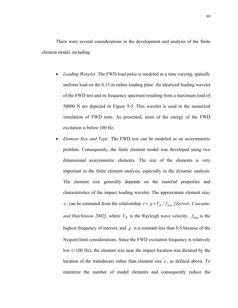
80

There were several considerations in the development and analysis of the finite

element model, including:

• Loading Wavelet: The FWD load pulse is modeled as a time varying, spatially

uniform load on the 0.15 m radius loading plate. An idealized loading wavelet

of the FWD test and its frequency spectrum resulting from a maximum load of

50000 N are depicted in Figure 5-5. This wavelet is used in the numerical

simulation of FWD tests. As presented, most of the energy of the FWD

excitation is below 100 Hz.

• Element Size and Type: The FWD test can be modeled as an axisymmetric

problem. Consequently, the finite element model was developed using two

dimensional axisymmetric elements. The size of the elements is very

important in the finite element analysis, especially in the dynamic analysis.

The element size generally depends on the material properties and

characteristics of the impact loading wavelet. The approximate element size,

e , can be estimated from the relationship max/ fVe R×< χ [Zerwer, Cascante,

and Hutchinson 2002], where RV is the Rayleigh wave velocity, maxf is the

highest frequency of interest, and χ is a constant less than 0.5 because of the

Nyquist limit considerations. Since the FWD excitation frequency is relatively

low (<100 Hz), the element size near the impact location was dictated by the

location of the transducers rather than element size e , as defined above. To

minimize the number of model elements and consequently reduce the

81

computational time of the forward model, the element size was increased

towards the boundaries of the model.

0 0.005 0.01 0.015 0.02 0.025 0.03 0.0350

1

2

3

4

5

6

7

8x 105

Time (sec)

Am

plitu

de (p

a)

0 50 100 150 200 2500

2

4

6

8

10

12x 106

Frequency (Hz)

Am

plitu

de (P

a)

Figure 5-5 - Time history (top) and frequency spectrum (bottom) of idealized time history wavelet.

• Overall Dimensions of the Model: To ensure the accuracy of the static finite

element analysis, consistent with the recommendations of previous studies,

the model boundaries were established at 10 m from the impact location.

Additionally, to ensure the accuracy of the dynamic analysis, infinite non-

reflecting boundaries were used at the perimeter of model. The relatively large

dimension of the model and non-reflecting infinite boundaries reduce the

effect of reflected waves from the boundaries and result in a more accurate

82

dynamic analysis. It should be mentioned that the infinite boundary elements

are also formulated to model far field response in a static analysis.

• Dynamic Analysis Time Step: The dynamic analysis of the FWD test was

performed using an explicit time integration method. The explicit dynamic

analysis procedure is based on the implementation of an explicit central

difference time integration rule. Unlike implicit dynamic analysis methods

that are unconditionally stable, the explicit dynamic analysis is only

conditionally stable. The time step in this type of analysis should be small

enough to prevent instability of the solution, which in simple terms means that

the time step should be small enough to prevent information to propagate over

more than one element per time step. This condition, which is sometimes

referred to as Courant, Friedrichs, and Lewy (CFL) condition, requires

selection of a time step t∆ such that: PVLt /<∆ , where PV is the

compressional wave velocity and L is the smallest distance between two

nodes in the model [Cook, Malkus, and Plesha, 1989].

Using the presented finite element model, the surface deflection time histories

from the dynamic linear elastic analysis by ABAQUS® due to the presented loading

wavelet are calculated and presented in Figure 5- 6. The material properties used in the

definition of the model are presented in Table 5-1. The presented pavement profile was

selected to be identical to the profiles considered in previous research studies, so that the

theoretical accuracy of finite element model can be further verified through a comparison

with the published deflection histories [Alkouhry et al, 2001]. The analysis was restricted

83

to 0.06 second because during the FWD test, pavement response is generally monitored

for this period of time. ABAQUS® automatically adjusts analysis time step to satisfy

CFL condition, however, the calculation results were reported at 0.001 second intervals.

As mentioned, the response of the presented pavement system under the idealized

loading wavelet, has been also previously studied by other researchers. To verify the

numerical accuracy of the developed finite element model, the model predictions were

compared to the published results. The published pavement deflection histories

[Alkhoury, 2001] for the same pavement model, as presented in Table 5-1, are presented

in Figure 5-7. These results are in close agreement with the obtained finite element

results presented in Figure 5-6. The predictions of dynamic models have been also

compared to actual filed measurements in general. In a recent study Loizos and Scarpas

[2005] have verified that the predictions of dynamic finite element models are in fact in

very good agreement with actual field measured values. Similar results were also

published by Zaghloul et al. [1994].

Table 5-1 - Geometrical and material properties used for definition of finite element model.

Material Type Thickness (m)

Elastic Modulus (MPa)

Rayleigh Damping

Ratio

Poisson’s Ratio

Mass Density (kg/m3)

Asphalt Concrete 0.15 1000 0.001 0.35 2300 Aggregate Base Course 0.25 200 0.001 0.35 2000

Subgrade infinity 100 0.001 0.35 1500

84

0 0.01 0.02 0.03 0.04 0.05 0.06-0.8

-0.7

-0.6

-0.5

-0.4

-0.3

-0.2

-0.1

0

0.1

Time (sec)

Def

lect

ion

(mm

)

r=0 mmr=200 mmr=300 mmr=450 mmr=600 mmr=900 mmr=1200 mmr=1500 mm

Figure 5-6 - Predicted pavement surface deflection time histories from ABAQUS® finite element model.

Figure 5-7 - Response of pavement surface deflection time histories [Alkhoury, 2001].

To be able to evaluate the probabilistic solution, modeling uncertainties should

also be defined. In general, evaluation of modeling uncertainties is a complex task and

further research is required to quantify such uncertainties. For examples presented in this

chapter, based on the experience, nominal modeling uncertainties were assigned for each

analysis.

85

Probabilistic Solution

It was shown in previous chapters that the probabilistic solution of the inverse

problem is the a posteriori probability, which can be presented as:

)()()( mmm MM λρσ = (5-2) where )(mλ is the likelihood function:

⎟⎠⎞

⎜⎝⎛ −+−−= −− ))(()(())((

21exp)( 11 mgdCCmgdkm obsdT

Tobsλ

(5-3)

In these equations, the model parameter(s) m is the parameter(s) of interest in the

problem, dC is the covariance of the data a priori information (assumed Gaussian) and

TC is the uncertainty in prediction of forward model )(mg (assumed Gaussian as well).

In this chapter, this problem is solved using the Monte Carlo solution scheme with

neighborhood approximation, as presented in Chapter 4. For backcalculation analysis

presented in this study the data were considered to be a single vector formed by

combining the data from individual receives.

Computational Time

The computational time for backcalculation analysis is directly proportional to the

number of forward model runs. In the probabilistic approach, the number of the forward

model runs depends on many factors, such as the number of model parameters, accuracy

required in defining the probabilities and accuracy in identifying the maximum point of

probabilities. The NA algorithm provides two variables to control the search effort and

define accuracy of the results. For FWD backcalculation using a three layer pavement

model, depending on the value of control parameters, the number of forward model runs

can vary significantly (approximately from 50 runs to 500 runs). Obviously, the higher

86

the required accuracy or the number of the model parameters, the higher the number of

forward model runs.

Backcalculation of Synthetic Test Data

Synthetic FWD Test Data

To be able to evaluate the performance of the probabilistic backcalculation

approach, the approach is initially implemented on a set of synthetic FWD test results,

where the material properties used for generation of the synthetic data are known. These

data sets were generated using the described dynamic finite element model above. The

material and geometric properties used in the generation of the synthetic data are the ones

presented in Table 5-1.

The presence of the shallow bedrock affects the FWD test results. Therefore, in

addition to the presented finite element model, where no bedrock was considered in

development of the model (i.e. deep bedrock), another set of synthetic data with the

similar finite element model was also generated, except that it was assumed that the

bedrock is at 2 m below the surface (i.e. shallow bedrock). Deflection time histories for

both these cases are depicted in Figure 5-8. Artificial, normally distributed random noise

with a maximum amplitude of one micron, which is a typical resolution of the FWD

displacement measurement [Dynatest, 1995], was added to these records to simulate

environmental noise in actual FWD test data and to avoid potential numerical problems.

The deflection bowls for the simulations with and without bedrock are also shown in

Figure 5-9. It should be emphasized that the deflection bowls are obtained from time

87

histories of dynamic model. The presented deflection bowls as well as the time histories

are used here as the synthetic FWD test results for input to the backcalculation routine.

0 0.01 0.02 0.03 0.04 0.05 0.06-0.8

-0.7

-0.6

-0.5

-0.4

-0.3

-0.2

-0.1

0

0.1

Time (sec)

Def

lect

ion

(mm

)

r=0 mmr=200 mmr=300 mmr=450 mmr=600 mmr=900 mmr=1200 mmr=1500 mm

0 0.01 0.02 0.03 0.04 0.05 0.06-0.8

-0.7

-0.6

-0.5

-0.4

-0.3

-0.2

-0.1

0

0.1

Time (sec)

Def

lect

ion

(mm

)

r=0 mmr=200 mmr=300 mmr=450 mmr=600 mmr=900 mmr=1200 mmr=1500 mm

Figure 5-8 - Synthetic FWD data for no bedrock (top) and shallow bedrock at 2 m below the surface (bottom).

Def

lect

ion

(mm

)

0 250 500 750 1000 1250 1500-0.7

-0.6

-0.5

-0.4

-0.3

-0.2

-0.1

0

Bedrock at 2 mNo Bedrock

Figure 5-9 - Deflection bowls for synthetic FWD data.

88

Backcalculation of Layer Modulus based on Deflection Bowl Using Linear

Static Forward Model

The first set of backcalculation analysis consists of backcalculation of layer

moduli based on the deflection bowl measurements for the pavement section with a deep

bedrock. The forward model in this backcalculation analyses was the static linear finite

element model presented previously. The data uncertainty was considered to follow a

Gaussian distribution with the mean equal to the observed value and a coefficient of

variation of two percent. Although present, no modeling uncertainty was considered for

this analysis.

One-dimensional kernel density estimates of marginal probability densities of the

layer moduli from the backcalculation analysis are presented in Figure 5-10. A

comparison between the observed deflection bowl and the defection bowl corresponding

to the most probable moduli values is also presented in the same figure. It can be

observed that, although there is a reasonably good match between the observed and

backcalculated deflection bowls, the backcalculated layer moduli are very different from

the values used in the generation of the synthetic data. This discrepancy is basically due

to modeling uncertainties that are not included in the backcalculation analysis. In other

words, the synthetic observed deflection bowl, as presented in Figure 5-9, was generated

using a linear dynamic finite element model. However, the backcalculation routine uses a

static model to backcalculate for layer moduli. Unless this discrepancy in modeling is

explicitly considered in the backcalculation, the final results would not be close to the

target values used in the generation of the deflection bowl. It should be mentioned that

89

this approach to backcalculation is similar to the current dominant practice of FWD

backcalculation, where the results of the FWD test (a dynamic test) are summarized in

terms of the deflection bowl and are backcalculated using a static forward model. Based

on this analysis, it can be observed that the static backcalculation, without an explicit

consideration of modeling uncertainty, results in incorrect backcalculated values.

The fact that the static backcalculation may produce incorrect results has been

previously acknowledged by other researchers. However, it is the general assumption that

the difference in the obtained results is relatively small. Obviously, for the example

presented here, this is not the case and this assumption should be further evaluated.

In the probabilistic backcalculation, the modeling uncertainties, can be explicitly

considered in the analysis. To illustrate such an approach, the modeling uncertainty for

this analysis has been evaluated by comparing the deflection bowls from static and

dynamic analyses of the same pavement model for a range of layer modulus values, as

presented in Table 5-2. The kernel density estimates of the absolute difference between

calculated deflections from dynamic and static analyses for each receiver are depicted in

Figure 5-11. The calculated histograms of the this absolute difference are also presented

in this figure.

Table 5-2 – Range of layer moduli values used for evaluation of modeling uncertainties using deflection bowls from static analysis.

Material Type Elastic Modulus Range (MPa) Asphalt Concrete 500~4000

Aggregate Base Course 50~400 Subgrade 50~400

90

0.5 1 1.5 2 2.5 3 3.5 4

x 109Asphalt Layer Modulus (Pa)

Mar

gina

l Pro

babi

lity

0.5 1 1.5 2 2.5 3 3.5 4

x 108Base Layer Modulus (Pa)

Mar

gina

l Pro

babi

lity

0.5 1 1.5 2 2.5 3 3.5 4

x 108Subgrade Modulus (Pa)

Mar

gina

l Pro

babi

lity

(a) (b) (c)

0 0.25 0.5 0.75 1 1.25 1.5-0.7

-0.6

-0.5

-0.4

-0.3

-0.2

-0.1

0

Receiver Offset (m)

Def

lect

ion

(mm

)

ObservedBackcalculated

(d)

Figure 5-10 - (a, b and c) Kernel density estimates of marginal a posteriori probabilities for the layer moduli obtained from the probabilistic backcalculation of the deflection bowl with the static forward model without considering modeling uncertainties and (d) comparison of the backcalculated deflection bowls for the pavement section with the most probable layer moduli and the observed data.

Correct Result

Correct Result

Correct Result

91

The modeling uncertainty at each receiver for input in the backcalculation

procedure can be evaluated by calculating the covariance of the difference between

calculated deflections from dynamic and static analyses for each receiver. Based on this

analysis, as a first estimate, a Gaussian distribution with a standard deviation of 0.1 mm

will be used to represent the modeling uncertainty for all receivers. It can be observed

that the evaluated modeling uncertainty is significantly higher than the data uncertainty.

The uncertainty in data was shown to be small, with a coefficient of variation of about 2

percent, where the coefficient of variation for modeling uncertainty ranges from 20 to

about 170 percent.

In the probabilistic approach with Gaussian data and model uncertainties, the

covariance representing the modeling uncertainties can be added to the data uncertainty

covariance. Using this approach, a new set of analysis was performed, which includes the

combined effect of data and modeling uncertainties. One-dimensional marginal

probability densities of the layer moduli from the backcalculation analysis are presented

in Figure 5-12. It can be observed that the obtained probabilities have significant spreads,

which indicated low reliability of the results. Based on these results, it can be concluded

that due to high modeling uncertainties, the backcalculation of modulus using a static

model is very unreliable.

92

0 0.1 0.2 0.3 0.4 0.5Absolute Difference for Receiver1 (mm)

Pro

babi

lity

0 0.1 0.2 0.3 0.4 0.5Absolute Difference for Receiver2 (mm)

Pro

babi

lity

0 0.1 0.2 0.3 0.4 0.5Absolute Difference for Receiver3 (mm)

Pro

babi

lity

0 0.1 0.2 0.3 0.4 0.5Absolute Difference for Receiver4 (mm)

Pro

babi

lity

0 0.1 0.2 0.3 0.4 0.5Absolute Difference for Receiver5 (mm)

Pro

babi

lity

0 0.1 0.2 0.3 0.4 0.5Absolute Difference for Receiver6 (mm)

Pro

babi

lity

0 0.1 0.2 0.3 0.4 0.5Absolute Difference for Receiver7 (mm)

Pro

babi

lity

0 0.1 0.2 0.3 0.4 0.5Absolute Difference for Receiver8 (mm)

Pro

babi

lity

Figure 5-11 – Histograms and kernel density estimate of the absolute difference between the calculated maximum deflections from dynamic and static analyses at each receiver location and . The area under each density estimate is equal to one unit. The histograms are scaled to fit in the same figure.

93

0.5 1 1.5 2 2.5 3 3.5 4

x 109Asphlat Layer Modulus (Pa)

Mar

gina

l Pro

babi

lity

0.5 1 1.5 2 2.5 3 3.5 4

x 108Base Layer Modulus (Pa)

Mar

gina

l Pro

babi

lity

0.5 1 1.5 2 2.5 3 3.5 4

x 108Subgrade Modulus (Pa)

Mar

gina

l Pro

babi

lity

(a) (b) (c)

0 0.25 0.5 0.75 1 1.25 1.5-0.7

-0.6

-0.5

-0.4

-0.3

-0.2

-0.1

0

Receiver Offset (m)

Def

lect

ion

(mm

)

(d)

Figure 5-12 - (a, b and c) Kernel density estimates of marginal a posteriori probabilities for the layer moduli obtained from the probabilistic backcalculation of the deflection bowl with the static forward model, which includes the modeling uncertainties, and (d) comparison of the backcalculated deflection bowls for the pavement section with the most probable layer moduli and the observed data.

Correct Result Correct

ResultCorrect Result

94

Backcalculation of Layer Moduli Based on Deflection Bowl Using Linear

Dynamic Forward Model

It was shown that due to significant modeling uncertainties, the results of FWD

deflection bowl backcalculation using static forward model are very unreliable. If instead

of a static model, a dynamic model is used, the discrepancy and uncertainty in the

modeling will be eliminated, and it is reasonable to expect that the analysis would

recover the correct layer moduli. This expectation is in fact verified by the analysis

results. Kernel density estimates of marginal probability densities for the layer moduli

obtained from the probabilistic deflection bowl backcalculation with a dynamic forward

model are presented in Figure 5-13. For this analysis, data uncertainty was considered to

follow a Gaussian distribution with the mean equal to the observed value and a

coefficient of variation of two percent. No modeling uncertainty was considered, because

the same model was used to generate both theoretical and observed deflection bowls. As

depicted, the backcalculation results have peaks at the correct modulus values. A

comparison of the observed and backcalculated deflection bowls are also presented in the

same figure.

By review of the presented results, it can be observed that, even though the data

uncertainty is very small (a coefficient of variation of two percent was used as presented

previously) and there is no modeling uncertainty (the same model was used in the

generation of theoretical and synthetic data), the backcalculated values have a relatively

large spread and display several peaks. This spread and multiple peaks can be related to

the sensitivity of the deflection bowl data to the layer modulus values.

95

0.5 1 1.5 2 2.5 3 3.5 4

x 109Asphalt Layer Modulus (Pa)

Mar

gina

l Pro

babi

lity

0.5 1 1.5 2 2.5 3 3.5 4

x 108Base Layer Modulus (Pa)

Mar

gina

l Pro

babi

lity

0.5 1 1.5 2 2.5 3 3.5 4

x 108Subgrade Modulus (Pa)

Mar

gina

l Pro

babi

lity

(a) (b) (c)

0 0.25 0.5 0.75 1 1.25 1.5-0.7

-0.6

-0.5

-0.4

-0.3

-0.2

-0.1

0

Receiver Offset (m)

Def

lect

ion

(mm

)

ObservedBackcalculated

(d)

Figure 5-13 - (a, b and c) Kernel density estimates of marginal a posteriori probabilities for the layer moduli obtained from the probabilistic backcalculation of the deflection bowl with the dynamic forward model and (d) comparison of the backcalculated deflection bowls for the pavement section with the most probable layer moduli and the observed data.

Correct Result

Correct Result

Correct Result

96

Deflection bowl backcalculation procedures rely heavily on deflection

measurements at discrete points. For the specific analysis presented here, eight discrete

deflection measurements were used to backcalculate three unknown modulus values. So,

it should be expected that any uncertainty in the deflection measurement and/or

theoretical modeling would translate into a relatively significant variation of

backcalculated moduli. This statement can be demonstrated in the probabilistic approach

by increasing the uncertainty in data. Figure 5-14 depicts the kernel density estimates of

marginal probabilities for the same problem with a combined data and modeling

uncertainty coefficient of variation of eight percent. It can be observed that the spread of

the backcalculated moduli has increased significantly. The increase in the spread

indicates that, if for any reason the uncertainty in data or model increases, the reliability

of backcalculation results based on the deflection bowl would decrease significantly.

97

0.5 1 1.5 2 2.5 3 3.5 4

x 109Asphalt Layer Modulus (Pa)

Mar

gina

l Pro

babi

lity

0.5 1 1.5 2 2.5 3 3.5 4

x 108Base Layer Modulus (Pa)

Mar

gina

l Pro

babi

lity

0.5 1 1.5 2 2.5 3 3.5 4

x 108Subgrade Modulus (Pa)

Mar

gina

l Pro

babi

lity

(a) (b) (c)

0 0.25 0.5 0.75 1 1.25 1.5-0.7

-0.6

-0.5

-0.4

-0.3

-0.2

-0.1

0

Receiver Offset (m)

Def

lect

ion

(mm

)

ObservedBackcalculated

(d)

Figure 5-14 -(a, b and c) Kernel density estimates of marginal a posteriori probabilities for the layer moduli obtained from the probabilistic backcalculation of the deflection bowl with the dynamic forward model with high model and data uncertainty and (d) comparison of the backcalculated deflection bowls for the pavement section with the most probable layer moduli and the observed data.

Correct Result

Correct Result

Correct Result

98

The heavy reliance of the deflection bowl backcalculation on a very small set of

data has resulted in difficulties in the deterministic backcalculation procedures, such as

inconsistency of the results from different programs and analysts for the identical a set of

data. As it has been shown, the a posteriori probabilities may have multiple peaks. In the

deterministic backcalculation procedures, presence of several peaks means that the

deterministic procedures can be trapped in any of the peaks and report the corresponding

value as the backcalculation result. This means that there is chance that the reported

values are not the correct values. This is a very serious problem, especially when the

uncertainty in data increases. Such an increase should be expected for actual FWD test

data, because for the experimental data, in addition to data uncertainty, there is always a

modeling uncertainty component. Therefore, it can be concluded that, although the

deflection bowl backcalculation using dynamic models can be used to correctly

backcalculate the moduli, the relatively low sensitivity of the moduli to data (or in other

words low information content of data) may produce a rather large uncertainty in the

backcalculated result.

Backcalculation of Layer Moduli Based on Deflection Time History Using

Linear Dynamic Time Domain Forward Model

Intuitively, deflection time histories of the FWD test carry significantly more

information regarding the pavement than the discrete deflection bowl measurements. So,

it is expected that the backcalculation procedures that use time histories should provide

more reliable results. This in fact can be observed from the backcalculation of the

synthetic test result on the pavement section with a deep bedrock using the dynamic

99

forward model. For this backcalculation analysis, the data uncertainty coefficient of

variation was selected to be two percent and no modeling uncertainty was considered,

because the same model was used in the generation of synthetic results, as well as

theoretical data. Kernel density estimates of marginal a posteriori probability densities for

the layer moduli obtained from the probabilistic backcalculation are presented in Figure

5-15. A comparison of the backcalculated deflection time histories for the pavement

section with the most probable layer moduli and the observed data are also presented in

the same figure. As presented, these results have much sharper peaks at the correct

moduli values. So, it can be concluded that using the complete deflection time history as

the data is a much more reliable approach in the FWD backcalculation. The main

practical problem in using this approach is its computational cost in terms of calculating

the dynamic response of the pavement. However, with a rapid increase in the available

computational power and availability of faster forward modeling approaches, the

additional computational cost should not be considered as a major obstacle.

100

0.5 1 1.5 2 2.5 3

x 109Asphalt Layer Modulus (Pa)

Mar

gina

l Pro

babi

lity

0.5 1 1.5 2 2.5 3 3.5 4

x 108Base Layer Modulus (Pa)

Mar

gina

l Pro

babi

lity

0.5 1 1.5 2 2.5 3 3.5 4

x 108Subgrade Modulus (Pa)

Mar

gina

l Pro

babi

lity

(a) (b) (c)

0 0.01 0.02 0.03 0.04 0.05 0.06-0.7

-0.6

-0.5

-0.4

-0.3

-0.2

-0.1

0

0.1

Time (sec)

Def

lect

ion

(mm

)

BackcakculatedObserved

(d)

Figure 5-15 - (a, b and c) Kernel density estimates of marginal a posteriori probabilities for the layer moduli obtained from the probabilistic backcalculation of the deflection time history with the dynamic forward model and (d) comparison of the backcalculated deflection time histories for the pavement section with the most probable layer moduli and the observed data. The two time histories are overlapping.

Correct Result

Correct Result

Correct Result

101

Backcalculation of Layer Moduli and Depth to Bedrock Based on Deflection

Time History Using Linear Dynamic Forward Model

The pavement response to FWD impact is remarkably different when a shallow

bedrock is present, compared to when it is not. Consequently, the backcalculation of

moduli should consider the effect of the bedrock. There is no direct indication of the

presence of a shallow bedrock in deflection bowl measurements. However, presence of a

shallow bedrock can be recognized by low amplitude reflections present at the later part

of a time record. Currently, available backcalculation procedures rely on the ability and

experience of the analyst to recognize presence of a shallow bedrock, estimate its depth,

and include its effect in the analysis.

Conceptually, the depth to bedrock can be considered as one of the model

parameters that should be resolved from the backcalculation analysis. Any prior estimates

of the depth to bedrock, if available, can also be included as a priori information. Using

this method, the solution of the backcalculation problem simultaneously provides the

backcalculated values of the depth to bedrock, as well as pavement layer moduli. To

evaluate such an approach, the backcalculation of time histories of the synthetic test with

a shallow bedrock was performed, where the depth to bedrock was considered to be one

of the model parameters. Marginal a posteriori probability densities for the layer moduli

and depth to bedrock obtained from the probabilistic backcalculation are presented in

Figure 5-16. A comparison of the backcalculated deflection time histories for the

pavement section with the most probable layer moduli and the observed data are also

presented in this figure.

102

0.5 1 1.5 2 2.5 3 3.5 4

x 109Asphalt Layer Modulus (Pa)

Mar

gina

l Pro

babi

lity

Den

sity

0.5 1 1.5 2 2.5 3 3.5 4Base Layer Modulus (Pa)

Mar

gina

l Pro

babi

lity

Den

sity

x1080.5 1 1.5 2 2.5 3 3.5 4

x 108Subgrade Modulus (Pa)

Mar

gina

l Pro

babi

lity

Den

sity

(a) (b) (c)

1 2 3 4 5 6 7 8 9 10Depth to Bedrock (m)

Mar

gina

l Pro

babi

lity

Den

sity

0 0.01 0.02 0.03 0.04 0.05 0.06-0.7

-0.6

-0.5

-0.4

-0.3

-0.2

-0.1

0

0.1

Time (sec)

Def

lect

ion

(mm

)

BackcalculatedObserved

(d) (e)

Figure 5-16 - (a, b, c and d) Kernel density estimates of marginal a posteriori probabilities for the layer moduli and depth to bedrock obtained from the probabilistic backcalculation of the deflection time histories with the dynamic forward model and (e) comparison of the backcalculated deflection time histories for the pavement section with the most probable layer moduli and the observed data.

Correct Result

Correct Result

Correct Result

Correct Result

103

As presented, these results have sharp peaks at the correct moduli and depth to

bedrock values, confirming the possibility of simultaneously backcalculating moduli and

depth to bedrock with low levels of uncertainty. However, the additional information (i.e.

the depth to bedrock) is obtained at the expense of additional computational cost required

to search a higher dimension model space and locate the “good” regions of the space.

This analysis demonstrates that the dynamic deflection time histories carry much more

information than deflection bowls and, thus, confirms that using time histories as the

input data is a much more reliable approach in the FWD backcalculation.

Backcalculation of Layer Moduli and Thickness Based on Deflection Time

History Using Linear Dynamic Forward Model

Theoretically, the thickness and moduli of pavement layers can be both

considered as the model parameters in a backcalculation analysis. Including the thickness

in backcalculation analysis increases the number of model parameters, which in turn

would require more computational effort in the search stage. Limited backcalculation

analyses performed as part of this research were not successful in recovering the correct

thickness and moduli and further work is required to investigate the possibility of

backcalculation of thickness and moduli from time history data.

Backcalculation Based on Velocity Time History

Most often, the transducers used in FWD testing do not directly measure the

pavement deflection. These transducers generally measure the particle velocity of the

104

pavement motion following the impact. The measured velocity history is then integrated

to evaluate the pavement deflection history. The integration introduces additional

uncertainties in the analysis. If the resolution of the transducers is low or the noise level

is high, such uncertainties can be significant. To reduce such uncertainties, the

backcalculation analysis can be performed using the velocity time histories as data.

For the backcalculation analysis presented in this research, there is no

fundamental difference between using the velocity time histories or the deflection time

histories. The deflection data has been historically used in FWD backcalculation mainly

because it is more tangible. However, if using the deflection data introduces additional

uncertainties; the backcalculation can be performed on the velocity level.

The feasibility of such analysis is illustrated here by the backcalculation of

velocity time histories of pavement during the synthetic FWD test. For this analysis,

similar to the previous analyses, the data uncertainty coefficient of variation was chosen

to be two percent. Marginal a posteriori probability densities for the layer moduli

obtained from the probabilistic backcalculation are presented in Figure 5-17. A

comparison of the backcalculated velocity time histories for the pavement section with

the most probable layer moduli and the observed data are also presented in the figure.

Based on the presented results, it can be observed that the velocity backcalculation can be

used to backcalculate the correct layer moduli with small uncertainty.

105

0.5 1 1.5 2 2.5 3 3.5 4

x 109Asphlat Layer Modulus (Pa)

Mar

gina

l Pro

babi

lity

0.5 1 1.5 2 2.5 3 3.5 4

x 108Base Layer Modulus (Pa)

Mar

gina

l Pro

babi

lity

0.5 1 1.5 2 2.5 3 3.5 4

x 108Subgrade Modulus (Pa)

Mar

gina

l Pro

babi

lity

(a) (b) (c)

0 0.01 0.02 0.03 0.04 0.05 0.06-0.08

-0.06

-0.04

-0.02

0

0.02

0.04

0.06

0.08

0.1

Time (sec)

Vel

ocity

(m/s

)

BackcalculatedObserved

(d)

Figure 5-17 - (a, b, and c) Kernel density estimates of marginal a posteriori probabilities for the layer moduli obtained from the probabilistic backcalculation of the velocity time histories with the dynamic forward model and (d) comparison of the backcalculated velocity time histories for the pavement section with the most probable layer moduli and the observed data.

Correct Result Correct

ResultCorrect Result

106

Backcalculation of FWD Test Data The objective of the analysis presented in this section is to demonstrate the

applicability of the presented probabilistic approach for backcalculation of the actual

FWD test results. To achieve this objective, time records of the actual tests are

backcalculated using a dynamic forward model to obtain the layer moduli. Details of the

analysis are presented in this section.

FWD Test Results

The test results used in this section were collected as a part of the FWD

monitoring program performed in the course of a research project on pavement material

characterization and seasonal variation of properties conducted jointly by Rutgers

University and Stantec, Inc. The details of the project and its results have been published

in a number of reports and papers [Zaghloul et al. 2006, Gucunski et al. 2004]. For the

analysis in this section, the results from the section No. 340507 of SPS-5 test site are

used. The load and deflection records for this test are shown in Figure 5-18. Inspection of

the recovered core at this section indicates that the thickness of the paving layer is about

0.36 m and it is underlain by a base layer of about 0.275 m thick. The presented data are

used as the input to the backcalculation analysis to obtain the layer moduli and

corresponding uncertainty measures based on the deflection time histories.

107

0 10 20 30 40 50 60-10

0

10

20

30

40

50

60

70

Time (msec)

Forc

e (K

N)

0 10 20 30 40 50 60-0.12

-0.1

-0.08

-0.06

-0.04

-0.02

0

0.02

time (msec)

Def

lect

ion

(mm

)

r=0 mmr=203 mmr=305 mmr=457 mmr=610 mmr=914 mmr=1219 mmr=1524 mm

Figure 5-18 - Measured loading history (top) and pavement response for FWD test.

Backcalculation Results

For this backcalculation analysis, the presented loading history was used as an

input to the analysis to model the test. The data uncertainty coefficient of variation for the

presented analysis was selected to be two percent and modeling uncertainty was

considered to be negligible. Both these assumptions will be examined in the next section.

Kernel density estimates of marginal a posteriori probability densities for the layer

moduli obtained from the probabilistic backcalculation are presented in Figure 5-19. A

108

comparison of the backcalculated deflection time histories for the pavement section with

the most probable layer moduli and the observed data are also presented in the same

figure. As presented, these results have sharp peaks at the moduli values. So, it can be

concluded that using the complete deflection time history as the data it is possible to

backcalculate the experimental FWD data for layer moduli. It should be mentioned that

the accuracy of these results should be further validated with a more extensive study.

A Discussion on Data and Modeling Uncertainties

For the presented analysis of experimental data, it was assumed that modeling

uncertainty is negligible and the data uncertainty coefficient of variation was selected to

be two percent. Due to many factors, there are modeling uncertainties in predictions of

forward models. An evaluation of such uncertainties is required before routine

application of the presented approach for backcalculation of experimental FWD

measurements. Some sources of uncertainty are discussed below.

Based on the presented time history records, the data uncertainties seem to be

much higher than assumed two percent. As presented in Figure 5-17, there are residual

deflections at the end of the record, which is not present in theoretical results. A possible

explanation for these residual displacements at the end of the record is that they are

numerical artifact produced as a result of a poor transducer resolution. As mentioned

previously, the response of the pavement during a FWD test is measured by geophones,

which measure the velocity. To obtain displacement records, the velocity records are

numerically integrated. Consequently, the poor resolution of the velocity records and/or

presence of noise, would translate to a poor quality of deflection records.

109

2 3 4 5 6 7 8 9

x 109Asphlat Layer Modulus (Pa)

Mar

gina

l Pro

babi

lity

0.2 0.4 0.6 0.8 1 1.2 1.4 1.6 1.8 2

x 109Base Layer Modulus (Pa)

Mar

gina

l Pro

babi

lity

0.5 1 1.5 2 2.5 3 3.5 4

x 108Subgrade Modulus (Pa)

Mar

gina

l Pro

babi

lity

(a) (b) (c)

0 0.01 0.02 0.03 0.04 0.05 0.06-0.12

-0.1

-0.08

-0.06

-0.04

-0.02

0

0.02

Time (sec)

Def

lect

ion

(mm

)

BackcalculatedObserved

(d)

Figure 5-19 -(a, b, and c) Kernel density estimates of marginal a posteriori probabilities for the layer moduli obtained from the probabilistic backcalculation of the experimental deflection time histories with the dynamic forward model and (d) comparison of the backcalculated deflection time histories for the pavement section with the most probable layer moduli and the observed data.

110

For the set of the data presented in Figure 5-17, the velocity time histories can be

calculated by differentiating the time history records. The velocity time history record for

the receiver at a zero offset distance is presented in Figure 5-20 as a typical result. The

poor resolution of the velocity record is evident from the jumps in the data. Such poor

quality may explain residual displacements in the deflection records, which ultimately

would affect the backcalculation results and increase the uncertainties. An alternative

explanation for the residual displacements can be the low frequency vibration of the

frame supporting the test apparatus. A thought understanding of the sources of

uncertainty requires a more detailed study. However, this brief discussion highlights the

necessity of quantifying the magnitude of the uncertainties in the data so that they can be

appropriately represented in probabilistic backcalculation.

0 10 20 30 40 50 60-0.01

-0.005

0

0.005

0.01

0.015

0.02

Time (msec)

Vel

ocity

(m/s

)

Figure 5-20 - Measured velocity time history record at receiver at zero offset.

111

Effect of Considering Dynamic Material Properties of Pavement Layers on Backcalculation Results

Dynamic Moduli and Damping of Pavement Layers

In FWD backcalculations, the pavement system is generally modeled as a layered

elastic system, where the layer thicknesses and moduli are the model parameters. In the

current practice, the layer thicknesses are often evaluated prior to the tests and are

considered as a given input for backcalculation. So, pavement layer moduli are the only

model parameters that should be evaluated in the backcalculation.

Since the FWD test is in principle a dynamic test, the evaluated pavement moduli

can not be treated as static elastic moduli of pavement layers. Furthermore, the dynamic

pavement response is affected by internal or material damping of pavement layers, which

should be included in the analysis.

Moduli of pavement layers vary considerably throughout the year based on

environmental factors and the type of pavement layers. However, for backcalculation

purposes, the moduli of the pavement layers are assumed constant during the very short

period of the test. The validity of this assumption is investigated here.

Granular Layers

Among the factors that affect the moduli of granular layers during the short period

of FWD test, strain level is the only important factor that can not be considered constant.

From the field experience, for good pavements, the strain levels during the FWD test are

generally below 0.1% for the paving layer and are in the order of 0.01% for granular

layers [Lozios, et. al. 2003]. The variation of modulus and damping of sands with strain

112

is presented in Figure 5-21 as representative of the typical behavior of granular layers.

Based on these graphs, for strain levels encountered during the FWD test, the modulus

and damping of the soil layers can essentially be considered constant and very close to

the low strain static modulus. Additionally, based on these results, a hysteretic damping

ratio of two to six percent is a good representative of the damping of granular pavement

layers.

Figure 5-21 - Variation of modulus (top) and damping (bottom) with shear strain for sands [Seed et. al. 1986]. F ′ indicates the ratio of the modulus at each frequency to the static modulus.

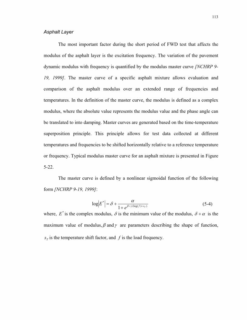
113

Asphalt Layer

The most important factor during the short period of FWD test that affects the

modulus of the asphalt layer is the excitation frequency. The variation of the pavement

dynamic modulus with frequency is quantified by the modulus master curve [NCHRP 9-

19, 1999]. The master curve of a specific asphalt mixture allows evaluation and

comparison of the asphalt modulus over an extended range of frequencies and

temperatures. In the definition of the master curve, the modulus is defined as a complex

modulus, where the absolute value represents the modulus value and the phase angle can

be translated to into damping. Master curves are generated based on the time-temperature

superposition principle. This principle allows for test data collected at different

temperatures and frequencies to be shifted horizontally relative to a reference temperature

or frequency. Typical modulus master curve for an asphalt mixture is presented in Figure

5-22.

The master curve is defined by a nonlinear sigmoidal function of the following

form [NCHRP 9-19, 1999]:

))(log(*

1log

TsfeE +++

+= γβ

αδ

(5-4)

where, *E is the complex modulus, δ is the minimum value of the modulus, αδ + is the

maximum value of modulus, β andγ are parameters describing the shape of function,

Ts is the temperature shift factor, and f is the load frequency.

114

Figure 5-22 - Typical modulus master curves for different asphalt mixtures [Clyne et. al. 2003].

The dominant portion of the excitation frequency of the FWD loading pulse is

generally below 100 Hz. As presented in the sample curves, for this range of frequencies,

the modulus can not be considered constant. Consequently, the assumption of constant

modulus during the backcalculation is not accurate, and effect of changes in modulus in

forward modeling and backcalculation should be studied and, if necessary, included in

the modeling and backcalculation.

The variation of internal damping of asphalt is much less than the variation of

modulus. Considering the small range of the damping ratios encountered, a constant

hysteresis damping ratio of two to five percent is representative of the damping of an

asphalt layer.

115

Concrete Layer

It is generally accepted that the modulus and damping of the cured concrete is

constant for the range of frequency and strain levels encountered during the FWD test.

Numerical Modeling of Dynamic Moduli and Damping

It has been shown that changes in frequency of excitation are the most important

factor affecting the pavement layer material properties during the short period of a FWD

test. So far, the moduli of pavement layers in presented backcalculation analysis were

considered to be independent of frequency and constant. This is the assumption generally

used in the current backcalculation procedures. However, as illustrated, the modulus of

asphalt is dependent on the frequency of excitation. Furthermore, the material damping in

finite element analysis was modeled as Rayleigh damping, which is a frequency

dependent damping. In other words, the damping ratio varies for different excitation

frequencies. However, as shown, the damping of pavement layers is generally constant.

The constant, frequency independent damping is modeled more appropriately using a

hysteresis damping model.

Modeling frequency dependent material properties in time domain is not straight

forward. The most convenient approach to include frequency dependent material

properties in the analysis is to use a frequency domain modeling approach. In the

frequency domain modeling, the response of the pavement system is obtained by a

synthesis of waveforms of many frequency components. In this research, a recently

developed frequency modeling technique, referred to as spectral element method, is used

to model the pavement response in the frequency domain. A general description of a

116

typical spectral element model of a pavement section and sample results are presented

below.

Frequency Domain Forward Model using Spectral Element Method

Spectral element method is a modeling approach for evaluation of the dynamic

response of horizontally layered media, such as pavements. Computationally, spectral

element method is a much more efficient method than the finite element modeling. In this

technique the solution is obtained by a synthesis of waveforms of many frequency

components, which are in part are obtained analytically. An overview of the

mathematical derivation and numerical implementation of this method is provided in

Appendix A. A more comprehensive explanation of this technique can be found in cited

references [Alkhoury, 2001, Rizzi and Doyle, 1992, Doyle, 1997].

For this study, a Matlab® code was developed to implement the spectral element

approach. The predicted surface deflection time histories evaluated by spectral element

method due to an idealized loading wavelet, presented previously, are shown in Figure 5-

23. Except for the damping ratios, the material properties used in the numerical

evaluation of the presented histories are similar to those used for the finite element

model. These properties are also listed in Table 5-3.

Table 5-3 - Geometrical and material properties used for development of spectral element results.

Material Type Thickness (m)

Elastic Modulus (MPa)

Hysteresis Damping

Ratio

Poisson’s Ratio

Mass Density (kg/m3)

Asphalt Concrete 0.15 1000 0.05 0.35 2300 Aggregate Base Course 0.25 200 0.02 0.35 2000

Subgrade infinity 100 0.02 0.35 1500

117

0 0.01 0.02 0.03 0.04 0.05 0.06-0.8

-0.7

-0.6

-0.5

-0.4

-0.3

-0.2

-0.1

0

0.1

Time (sec)

Def

lect

ion

(mm

)

r=0 mmr=200 mmr=300 mmr=450 mmr=600 mmr=900 mmr=1200 mmr=1500 mm

Figure 5-23 - Predicted pavement surface deflection time histories from linear spectral element analysis.

Comparison of Time and Frequency Domain Models

The predicted surface deflections from time domain and frequency domain

models for the pavement system in previous sections are compared in Figure 5-24. Since

tow models use different damping models, the results were not expected to match and no

attempt was made to vary the damping ratio to match them. However, the results are a

qualitative verification of the modeling approaches. As presented, the two results are in a

very good agreement. The slight difference in the predicted response is due to the

difference in the formulation of damping in time and frequency domain analyses, as

discussed previously. In the time domain, damping is modeled as Rayleigh damping,

where as in the frequency domain, damping is modeled as hysteresis damping. The

hysteresis damping is constant through out the analysis, but Rayleigh damping varies

depending on the frequency of excitation. Effects of this difference on the

backcalculation results are investigated in the next section.

118

0 0.01 0.02 0.03 0.04 0.05 0.06-0.8

-0.7

-0.6

-0.5

-0.4

-0.3

-0.2

-0.1

0

0.1

Time (sec)

Def

lect

ion

(mm

)

Finite Element

Spectral Element

Figure 5-24 - Comparison of predicted surface defections at different receiver location from time domain and frequency domain models.

Backcalculation of Layer Moduli Based on Deflection Time History Using

Linear Dynamic Frequency Domain Forward Model

It has been shown that due to the difference in the damping model, there will be

differences in the analysis results for the same pavement system using time or frequency

domain models. The general assumption in the backcalculation analysis presented so far

was that due to low sensitivity of the pavement response to damping ratios, the difference

in the damping model is not expected to be a major source of discrepancy in

backcalculation results. To evaluate this assumption, a backcalculation analysis was

performed, where the pavement deflection time histories obtained from the finite element

analysis were used as synthetic data and the backcalculation was done using a spectral

element forward model. The synthetic data was presented previously in Figure 5-8. In

this analysis, it has been assumed that the modeling uncertainty is negligible. In other

words, it has been assumed that the spectral element results are comparable to finite

element results. Marginal a posteriori probability densities for the layer moduli obtained

119

from the probabilistic backcalculation are presented in Figure 5-25. A comparison of the

backcalculated deflection time histories for the pavement section with the most probable

layer moduli and the observed data are also presented in the figure.

It can be observed that, even though there is good match between the observed

and backcalculated time histories, the backcalculated layer moduli are not correct. This

result can be explained by the difference between the spectral element and finite element

time history results. Consequently, the modeling uncertainties should be included in the

analysis. This result is important because it highlights the importance of considering the

modeling uncertainties in the analysis.

120

0.5 1 1.5 2 2.5 3 3.5 4

x 109Asphalt Layer Modulus (Pa)

Mar

gina

l Pro

babi

lity

0.5 1 1.5 2 2.5 3 3.5 4

x 108Base Layer Modulus (Pa)

Mar

gina

l Pro

babi

lity

0.5 1 1.5 2 2.5 3 3.5 4

x 108Subgrade Modulus (Pa)

Mar

gina

l Pro

babi

lity

(a) (b) (c)

0 0.01 0.02 0.03 0.04 0.05 0.06-0.7

-0.6

-0.5

-0.4

-0.3

-0.2

-0.1

0

0.1

Time (sec)

Def

lect

ion

(mm

)

ObservedBackcalculated

(d)

Figure 5-25 - (a, b and c) Kernel density estimates of marginal a posteriori probabilities for the layer moduli obtained from the probabilistic backcalculation of the deflection time history with the spectral element forward model and (d) comparison of the backcalculated deflection time histories for the pavement section with the most probable layer moduli and the observed data.

Correct Result

Correct Result Correct

Result

121

Pavement Response with Dynamic Moduli

For the FWD test, modulus and damping of granular and cement concrete layers,

and damping of on asphalt layer can be considered constant in forward modeling and

backcalculation of pavement layer moduli. However, the asphalt layer modulus is

strongly dependent on frequency of excitation for the frequency range of interest in FWD

tests. To study the effect of variable moduli on the analysis results, a dynamic analysis

using spectral element method was performed, where the frequency modulus master

curve were used to model the frequency dependent asphalt modulus. Except for damping

and modulus values, the geometry and material properties used in the analysis are

basically the same properties used in the finite element and spectral element analyses

presented. The modulus and damping values used in this analysis are presented in Table

5-4. For this analysis, the asphalt modulus was calculated at each frequency based on the

sample modulus master curve presented in Figure 5-26. The predicted surface deflection

time histories due to an idealized loading wavelet are shown in Figure 5-27.

Table 5-4 – Modulus and damping values used for numerical evaluation of spectral element analysis.

Material Type Elastic Modulus (MPa) Damping Ratio Asphalt Concrete See Master Curve in Figure

5-26 0.05

Aggregate Base Course 200 0.02 Subgrade 100 0.02

122

10.0

100.0

1000.0

10000.0

100000.0

1.E-04 1.E-02 1.E+00 1.E+02 1.E+04 1.E+06

Frequency (Hz)

Modulus (MPa)

Constant Modulus

|E*|

(MPa

)

Figure 5-26 – Sample modulus curve and constant modulus line used for numerical evaluation of the pavement response with spectral element approach. The curve parameters are 8.2=α ,

44.0−=β , 48.1−=δ , , 56.0−=γ and 0=TS (See equation 5-4).

0 0.01 0.02 0.03 0.04 0.05 0.06-0.45

-0.4

-0.35

-0.3

-0.25

-0.2

-0.15

-0.1

-0.05

0

0.05

Time (sec)

Def

lect

ion

(mm

)

r=0 mmr=200 mmr=300 mmr=450 mmr=600 mmr=900 mmr=1200 mmr=1500 mm

Figure 5-27 - Predicted pavement surface deflection time histories from spectral element analysis with dynamic asphalt layer modulus.

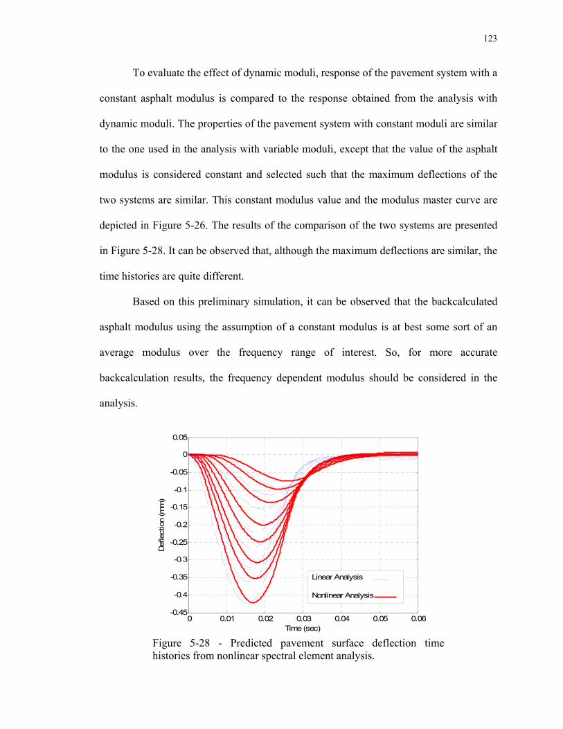
123

To evaluate the effect of dynamic moduli, response of the pavement system with a

constant asphalt modulus is compared to the response obtained from the analysis with

dynamic moduli. The properties of the pavement system with constant moduli are similar

to the one used in the analysis with variable moduli, except that the value of the asphalt

modulus is considered constant and selected such that the maximum deflections of the

two systems are similar. This constant modulus value and the modulus master curve are

depicted in Figure 5-26. The results of the comparison of the two systems are presented

in Figure 5-28. It can be observed that, although the maximum deflections are similar, the

time histories are quite different.

Based on this preliminary simulation, it can be observed that the backcalculated

asphalt modulus using the assumption of a constant modulus is at best some sort of an

average modulus over the frequency range of interest. So, for more accurate

backcalculation results, the frequency dependent modulus should be considered in the

analysis.

0 0.01 0.02 0.03 0.04 0.05 0.06-0.45

-0.4

-0.35

-0.3

-0.25

-0.2

-0.15

-0.1

-0.05

0

0.05

Time (sec)

Def

lect

ion

(mm

)

Linear Analysis

Nonlinear Analysis

Figure 5-28 - Predicted pavement surface deflection time histories from nonlinear spectral element analysis.

124

Finally, for the modeling and backcalculation of FWD test results it has been

assumed throughout this study that the material response is elastic and there is no plastic

deformation during the test. This is certainly a reasonable assumption for the level of

FWD loading. However, under the combination of heavy loads, weak pavement system

and/or high temperatures, plastic deformations of pavement layers may occur, which

invalidate this assumption. These extreme cases were not considered in this study.

Summary In this chapter, the probabilistic backcalculation of FWD test results was

introduced, formulated and the results of the probabilistic backcalculation of synthetic

test data using different backcalculation methods were presented as a better approach to

the FWD backcalculation. The probabilistic backcalculation was then applied to different

methods of backcalculation, such as static and dynamic backcalculation and the results

were compared. Based on the presented results, it was shown that, although very popular,

the static backcalculation procedures fail to capture the essential dynamic nature of the

test and consequently can not be relied upon for accurate backcalculation. Through the

comparison of two different sets of deflection bowl backcalculation using the dynamic

forward model, it was also demonstrated that there is little redundancy in dynamic

deflection bowl backcalculation procedures, which can produce large uncertainties in the

obtained backcalculation results. It was also shown that the dynamic deflection time

history backcalculation offers the best and most reliable approach in FWD

backcalculation. The application of this approach was illustrated both on synthetic and

125

experimental test data. It was also shown that, at least in the case of synthetic data, the

deflection time histories carry enough information to simultaneously backcalculate layer

moduli and the depth to bedrock. However, such additional information is obtained at a

higher computational cost required for a more thorough search of the model space.

Finally, the effect of frequency dependent layer material properties on the predicted

deflection time histories was investigated. It was shown that such effects can be

significant and produce discrepancies in the backcalculation results. A complete

understanding of these effects and techniques to include them in the backcalculation

analysis requires further research.

References ABAQUS (2005), Hibbitt, Karlsson, and Sorensen, Providence, RI. Al-khoury, R., Scarpas, A., Kasbergen, C., Blaauwendraad, J. (2001a), “Spectral

Element Technique for Efficient Parameter Identification of Layered Media: Part I: Forward Model”, International Journal of Solids and Structures, Vol. 38.

Al-khoury, R., Scarpas, A., Kasbergen, C., Blaauwendraad, J. (2001b), “Spectral Element Technique for Efficient Parameter Identification of Layered Media: Part II: Inverse Calculations”, International Journal of Solids and Structures, Vol. 38.

ASTM International, (1996), “ASTM D4694-96, Standard Test Method for Deflections with a Falling-weight-type Impulse Load Device”, American Society for Testing and Material (ASTM), Philadelphia, PA.

ASTM International, (2003), “ASTM D4695-03, Standard Guide for General Pavement Deflection Measurements”, American Society for Testing and Material (ASTM), Philadelphia, PA.

Bentson, R.A., Nazarian, S., Harrison, A. (1989), “Reliability of Seven Nondestructive Pavement Testing Devices”, Nondestructive testing of pavement and Backcalculation of moduli, American Society for Testing and Material (ASTM) Special Technical Publication 1198, ASTM, Philadelphia, PA.

Boddapati, K.M., and Nazarian, S. (1994), “Effects of Pavement-Falling Weight Deflectometer Interaction on Measured Pavement Response”, Nondestructive testing of pavement and Backcalculation of moduli – Second Volume, American Society for Testing and Material (ASTM) Special Technical Publication 1198, ASTM, Philadelphia, PA.

126

Bush, A. J. III, and Baladi, G.Y. (Editors) (1989), “Nondestructive testing of pavement and Backcalculation of moduli”, American Society for Testing and Material (ASTM) Special Technical Publication 1026, ASTM, Philadelphia, PA.

Cook R., Malkus D., Plesha M. (1989), “Concepts and Application of Finite Element Analysis” John Wiley & Sons, New York, NY.

Clyne R., Li, X., Marasteanu, M. O., Skok E. L. (2003), “ Dynamic and Resilient Modulus of MN/DOT Asphalt Mixtures” Report No. MN/RC-2003-09, Minnesota Department of Transportation, St. Paul, MN.

Doyle, J.M. (1997), “Wave Propagation in Structures”, Springer-Verlag, New York, NY.

Dynatest, (1995), “Dynatest 8081 HWD Test System – Owners Manual”, Dynatest Consulting Inc., Starke, FL.

ELMOD, (2001), “ELMOD Pavement Evaluation Manual (Version 4.5)”, Dynatest, Denmark.

Foinquinos, R., Roesset, J. M., and Stokoe, K.H. (1995), “Response of pavement systems to dynamic loads imposed by nondestructive tests” Transportation Research Record, n 1504, p 57-67.

Gucunski, N., Hadidi, R., Maher, A., and Vitillo, N. (2004), “Seismic Pavement Evaluation in Development of Seasonal Variation Models of Pavement Properties”, 5th International Conference on Case Histories in Geotechnical Engineering, New York, NY.

Haskell, N.A. (1953), “The Dispersion of Surface Waves on Multilayered Media”, Bulletin of Seismological Society of America, Vol. 43, 17-34.

Kausel, E. and Roesset, J. M. (1981), “Stiffness Matrices for Layered Soils”, Bulletin of Seismological Society of America, Vol. 71, 1743-1761.

Mamlouk, M.S. (1987), “Dynamic Analysis of Multilayered Pavement Structures – Theory, Significance and Verification”, Proceedings of 6th International Conference on Structural Design of Asphalt Pavements, Ann Arbor, Michigan.

Michalak, C.H., and Scullion, T., (1995), “MODULUS 5.0: User Manual”, Research Report 1987-1, Texas Transportation Institute, Texas A&M University, College Station, TX.

Lozios A., Boukovalas, G., and Karlaftis, A. (2003), “Dynamic Stiffness Modulus for Pavement Subgrade Evaluation” Journal of Transportation Engineering, Vol 129, No. 4.

Lozios, A., and Scarpas, T., (2005), “Verification of Falling Weight Deflectometer Backanalysis Using Dynamic Finite Elements Simulation”, The International Journal of Pavement Engineering, Vol. 6, No. 2.

National Cooperative Highway Research Program (NCHRP) (1999), ‘‘NCHRP 9-19, superpave support and performance models management, advanced AC mixture material characterization models framework and laboratory test plan.,’’ Final Report, submitted by Superpave Models Team, Dr. M. W. Witczak, Project Principal Investigator, Arizona State University, Tucson, AZ.

Rizzi, S.A. and Doyle, J.F. (1992), “Spectral Analysis of Wave Motion in Plane Solids with Boundaries”, Trans. of ASME, Journal of Vibration and Acoustics, Vol 114, No. 2, pp. 133-140.

127

Roesset, J. M., Stokoe, K. H. II, Send, C.R. (1995), “Determination of Depth to Bedrock from Falling Weight Deflectometer Test Data”, Transportation Research Record, Vol. 1504.

Seed, H. B., Wong, R. M., Idriss, I. M., and Tokimatsu, K. (1986), “Moduli and Damping Factors for Dynamic Analysis of Cohesionless Soils”, Journal of the Soil Mechanics and Foundation Division, Vol. 112, pp. 1016-1032.

Sebaaly, B. E., Davies, T. G., Mamlouk, M. S. (1985) “Dynamics of Falling Weight Deflectometer”, Journal of Transportation Engineering, ASCE, Vol. 3, No. 6.

Tayabji, S.D., and Lukanen, E.O. (Editors) (2000), “Nondestructive testing of pavement and Backcalculation of moduli – Third Volume”, American Society for Testing and Material (ASTM) Special Technical Publication 1375, ASTM, Philadelphia, PA.

Taylor B. N. and Kuyatt C. E. (1994), “Guidelines for Evaluation and Expressing Uncertainty of NIST Measurement Results”, Technical Note 1297, United States National Institute of Standards and Technology (NIST), United States Department of Commerce, Washington, DC.

Thomson, W.T., (1950), “Transmission of Elastic Waves through a Stratified Solid Media”, Journal of Applied Physics, Vol. 21, p. 89-93.

Uzan, J. (1994), “Advanced Backcalculation Techniques”, Nondestructive testing of pavement and Backcalculation of moduli – Second Volume, American Society for Testing and Material (ASTM) Special Technical Publication 1198, ASTM, Philadelphia, PA.

Von Quintus, H.L., Bush, A. J. III, and Baladi, G.Y. (Editors) (1994), “Nondestructive testing of pavement and Backcalculation of moduli – Second Volume”, American Society for Testing and Material (ASTM) Special Technical Publication 1198, ASTM, Philadelphia, PA.

Zaghloul, S.M., White, T.D. Drenevich, V.P., and Coree, B., (1994), “Dynamic Analysis of FWD Loading and Pavement Response Using a Three Dimensional Dynamic Finite Element Program”, Nondestructive testing of pavement and Backcalculation of moduli – Second Volume, American Society for Testing and Material (ASTM) Special Technical Publication 1198, ASTM, Philadelphia, PA.

Zaghloul, S.M., Gucunski, N., Jackson, H., and Hadidi, R. (2006), “Material Characterization and Seasonal Variation in Material Properties”, Report No. FHWA-NJ-2005-024, New Jersey Department of Transportation, Trenton, NJ.

Zaghloul S. M., Hoover, T., Swan, D. J., Vitilli, N., Sauber, R., and Jumikis, A. (2004), “Enhancing Backcalculation Procedures Through Consideration of Thickness Variability” Transportation Research Record, No. 1869, pp. 80-87.

Zerwer, A., Cascante, G., and Hutchinson, J. (2002), “Parameter Estimation in Finite Element Simulation of Raleigh Waves”, Journal of Geotechnical and Environmental Engineering, ASCE, 128(3).

128

6 Application Two: Model Calibration Based On Geotechnical Instrument Measurements

Introduction In design and construction problems in geotechnical engineering, there are always

elements of uncertainty due to different factors, such as the uncertainty in soil parameters

and/or construction sequence. To reduce the potential risk from the uncertainties that are

not included in the design, many important geotechnical engineering projects use an

observational method towards design and management of the project. The observational

method, which its development is generally attributed to Terzaghi [Casagrande, 1965,

Peck, 1969], can be described by the following steps:

• Assess probable and adverse outcomes for the design,

• Establish key parameters for observation,

• Calculate observational parameters under probable and adverse conditions

using predictive models,

• Measure observational parameters and compare them to calculations,

• Calibrate the predictive model based on the measured observational

parameters, and

129

• Change the design as needed.

Implementing the observational method is not a trivial task due to many

limitations in the ability to predict the ground response and/or monitor the desired

parameter. This is especially important for the projects, where the complexity of the

factors involved limits the ability of an engineer to evaluate the monitoring results and

outcomes without the help of predictive models. So, the development of a representative

model and its calibration is one of the important steps in implementing the observational

approach.

Model calibration is a classical example of an inverse problem, which can be

solved using the probabilistic approach. This chapter introduces the probabilistic

approach to the solution of inverse problems as a tool in calibration of the predictive

models and implementation of the observational method. Model calibration has been

historically performed by comparison between the observed and predicted model

responses and adjustment of the model parameters to obtain a reasonable match. Once

there is a good match between the observed and predicted responses, the model

parameters are considered to represent the true ground parameters, and the model is

considered calibrated. However, in this approach to calibration, effects of uncertainties in

observations and model predictions are not included in the analysis. This affects the

calibration analysis and consequently the model predictions for future measurements.

Using the probabilistic approach, uncertainties in the calibration process can be

quantified and their effects on the model predictions can be studied.

130

In this chapter, a landfill redevelopment project is used as an example to

demonstrate how the probabilistic approach to the solution of inverse problems can be

used to calibrate a predictive model and complement the application of the observational

method in geotechnical engineering. Although the main focus of this chapter is on

calibration based on the settlement data, the same approach can be used in different

contexts and for different problems with different types of measurements. Following this

introduction, an overview of the mentioned landfill redevelopment project is presented

and the need for model calibration and implementation of the observational method is

highlighted. The calibration of a settlement prediction model using the probabilistic

approach is then outlined and formulated. Finally, the results of the analysis are presented

and discussed.

Background

Project Overview

In a large scale landfill redevelopment project on several landfills in Northern

New Jersey, it was decided early on that some development features, including some of

the light structures, would be supported on shallow foundations over the landfill material,

which is underlain by a peat, organic silt, and deep varved clay strata. This decision was

justified because the costs for relocating landfill materials would be prohibitive and the

depth to competent bearing material makes deep foundation systems uneconomical. This

type of construction is in contrast to common practice of landfill development, which

relies on deep foundations to support structures planned for the project. Generally, due to

expected long term biodegradation settlement of landfill materials, most of the landfill

131

development projects to date are limited to types of construction that are not very

sensitive to settlement of the landfill materials, such as golf courses and parks. However,

the feasibility of shallow foundation construction for this project was justified by

considering the limited thickness of the landfill, the significant age of the landfill

materials, and the limited amount of gas being generated.

To limit the long term settlements from the compression of the landfill material

and underlying peat, organic silt, and varved clay strata, in addition to implementation of

an extensive environmental remediation program to address environmental concerns,

implementation of an intensive ground improvement program was anticipated. The

ground improvement program consisted of dynamic compaction of the landfill material, a

surcharge program to pre-compress the landfill material and the underlying peat, organic

silt, and varved clay strata, and the placement of controlled compacted fill of sufficient

thickness to provide a significant separation between the bottom of the proposed footings

and the top of the improved waste layer. Further details about the project and ground

improvement program can be found in the published literature [Lifrieri, et al. 2006a,

Lifrieri et al., 2006b].

At this time, the initial phase of this project, which consists of the development of

a 10 acre parcel of the project site, is completed. However, other phases of the project are

currently underway. The focus of this chapter is on the initial 10 acre parcel of the

project. The envisioned development plan for this landfill parcel consists of construction

of mid-rise residential and commercial real estate. The portion of the development that

will not be pile supported generally consists of parking areas, roadways, and settlement

sensitive landscaping features. To avoid future settlement related issues for these

132

features, a settlement criterion for the design of the ground improvement program was

adopted, which specifies limiting the long term total site settlement in 10 years to a

maximum of three inches.

Site Conditions

The soil borings performed within the project site indicated that the landfill

material, nine to 12 feet thick, is covered with a two to three foot layer of fill material of

various types. This waste layer is underlain by a peat and organic silt stratum with an

average thickness of five to ten feet. However, at limited portions of the project site, this

stratum is as thick as 25 feet. This organic stratum lie on top of a 110 to 140 feet thick

deposit of varved clay, which in turn rests on top of the glacial till and bedrock.

Geotechnical laboratory test results indicate that, except for the top desiccated portion of

the varved clay stratum of about five to ten foot thick, the varved clay is normally

consolidated and is very soft. A sketch of the generalized subsurface profile is depicted in

Figure 6-1.

133

Figure 6-1 – Sketch of the generalized subsurface profile

Ground Improvement Program

The ground improvement program consists of dynamic compaction (DC) to

improve the compression characteristics of the existing waste layer, followed by the

placement of 12 feet of surcharge fill over the proposed site grades to improve the

strength of the underlying peat, organic silt, and soft clay strata and to reduce post

construction long term settlements resulting from the settlement of these strata. To

monitor and verify the performance of the surcharge program, an instrumentation

program was designed for the project site. The instrumentation program included

installation and monitoring of magnetic extensometers, borros anchors, settlement plates,

vibrating wire piezometers, stand pipe piezometers, and inclinometers.

Peat/Organic Silt – 5~10 ft

Glacial Till/Bedrock

Soft Varved Clay – 110~140 ft

Stiff Clay – 5~10 ft

Landfill Material – 9~12 ft

Fill – 2~3 ft

134

To predict the future site response both during and after the construction and

validate the satisfactory performance of the surcharge loads, a predictive model was

developed and the ground settlement response was used to calibrate it. The calibrated

model was then used to predict the long term settlement of the site. The following section

presents the basic elements used in the analysis, formulates the probabilistic approach to

the problem, and demonstrates how the probabilistic approach offers advantages in model

calibration.

Development of Predictive Model and Calibration Measurements

Development of Predictive Model

A plan of the site along with the location of the borings and installed monitoring

instruments is presented in Figure 6-2. To evaluate the settlement and verify the

performance of the surcharge, a two dimensional predictive model of the site was

developed using Plaxis® software. The model geometry was developed based on the

borings performed at the project site along the cross section shown in Figure 6-2. The

developed model geometry is depicted in Figure 6-3.

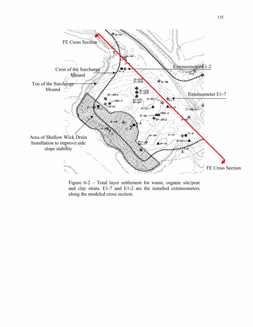
135

Figure 6-2 – Total layer settlement for waste, organic site/peat and clay strata. E1-7 and E1-2 are the installed extensometers along the modeled cross section.

FE Cross Section

FE Cross Section

Area of Shallow Wick Drain Installation to improve side

slope stability

Crest of the Surcharge Mound

Toe of the Surcharge Mound

Extensometer E1-2

Extensometer E1-7

136

Figure 6-3 – Geometry of developed finite element predictive.

Soft Clay Layer 3

Fill Waste Organics

Stiff Clay Layer

Till/Rock Soft Clay Layer 4

Distance (ft)

Elev

atio

n (f

t)

Soft Clay Layer 2

Soft Clay Layer 1

Extensometer E1-2

Extensometer E1-7

137

To model the fill placement activities, the stage construction analysis option in

Plaxis® was used. Fill placement at different locations along the cross section took place

at slightly different schedules. The loading history at two points along the cross section is

presented in Figure 6-4. This loading sequence was idealized for the development of the

model. The idealized loading sequence used in the model development is also presented

in Figure 6-4. A close up of the loading stages in the finite element model is shown in

Figure 6-5.

0 50 100 150 200 250 3000

2

4

6

8

10

12

14

Time (day)

Fill

Hei

ght (

ft)

Timeline at E1-2Timeline at E1-7Idealized Timeline

Figure 6-4 – Fill placement timeline at two points along the cross section and idealized fill placement timeline and stages used for model development.

Figure 6-5 – Close up view of idealized loading stages.

Stage 3 Stage 2 Stage 1

Existing Fill

Loading Stage 1

Loading Stage 2

Loading Stage 3

138

Material properties for the initial development of the predictive model were

selected based on the available site specific laboratory test results and published literature

pertaining to the type of soils encountered at the project site. The initial material

properties are listed in Table 6-1.

Measurement Results

The observed settlement of the waste, organics, and clay strata from monitoring of

extensometers E1-2 and E1-7 along the modeled section are presented in Figure 6-6. The

location of these extensometers is also indicated on the developed model presented in

Figure 6-2. The presented ground settlement response will be used to calibrate the

predictive model. Once the model is calibrated it was used to predict the future response

of the site under the applied loads.

0 50 100 150 200 250 300-0.8

-0.7

-0.6

-0.5

-0.4

-0.3

-0.2

-0.1

0

0.1

Time (day)

Set

tlem

ent (

ft)

WasteOrganics Silt/PeatSoft Clay

Figure 6-6 – Total layer settlement for waste, organic silt/peat and clay strata from extensometer measurements along the modeled cross section (Extensometer E1-2 and E1-7).

139

Table 6-1 – Initial material properties used for development of predictive model. (A) (B) (C) (D) (E) (F) (G) (H) (I) (J) (K) (L) (M)

Material Model unsatγ kg/m3 (pcf)

satγ kg/m3 (pcf)

yk m/sec (ft/d)

xy kk /

υ sV m/s

(ft/s)

c KPa (psf)

φ OCR cC ′ rC ′ αC ′

Fill MC 1922 (120)

2002 (125)

3.52E-6 (1)

1 0.3 225 (750)

4.8 (100)

34 - - - -

Waste SSC 1041 (65)

1521 (95)

10.6E-9 (3E-3)

1 - - 9.6 (200)

30 1 0.14 0.014 0.0014

Organics SSC 961 (60)

1441 (90)

1.06E-9 (3E-4)

1 - - 19.2 (400)

20 1 0.34 0.034 0.017

Stiff Clay MC 1762 (110)

1922 (120)

2.12E-9 (6E-4)

3 0.3 150 (500)

71.8 (1500)

23 - - - -

Soft Clay 1 SSC 1601 (100)

1762 (110)

2.12E-9 (6E-4)

3 - - 14.4 (300)

23 1 0.1 0.01 0.004

Soft Clay 2 SSC 1601 (100)

1762 (110)

1.76E-9 (5E-4)

3 - - 23.9 (500)

23 1 0.2 0.02 0.008

Soft Clay 3 SSC 1601 (100)

1762 (110)

3.18E-9 (9E-4)

3 - - 33.5 (700)

23 1 0.3 0.03 0.012

Soft Clay 4 SSC 1601 (100)

1762 (110)

1.06E-9 (3E-4)

3 - - 43.1 (900)

23 1 0.2 0.02 0.008

Table Legend: Independent Model Parameter for Calibration Dependent Model Parameter for Calibration

(A) Material Model: MC –Mohr-Coulomb Material Model, SSC–Soft Soil Creep Material Model (Plaxis, 2005), (B) Unit weight, (C) Saturated unit weight, (D) Permeability in vertical direction (E) Ratio of vertical to horizontal permeability, (F) Poisson’s ration, (G) Shear wave velocity, (H) Cohesion, (I) Friction angle, (J) Over consolidation ratio, (K) Strain based compression index, (L) Strain

based recompression index, (M) Strain based secondary compression index.

140

Initial Model Predictions

The predicted model response using initial material properties at E1-2 and E1-7

extensometer locations is depicted in Figure 6-7. For a comparison, the measured

response of the site at the same locations is depicted in the same figure. It can be

observed that, even though the material properties for the model are obtained from the

site specific laboratory test results, the predicted site response is very different than the

observed response, which highlights the need for model calibration.

Model Parameters

A fundamental step in the solution of any inverse problem, including the

calibration problem presented, is the selection of model parameters or parameterization.

Due to a relatively short span of settlement monitoring used for model calibration, the

presented site response can be considered to be essentially representative of the primary

consolidation of subsurface strata. Therefore, it is logical to expect that the response can

be adequately described by the compression indices and permeability coefficients of

subsurface strata. Based on this logic, the compression indices and permeability

coefficients of waste, organics, and first sublayer of soft clay strata were selected as the

model parameters. Since all four soft clay sublayers represent one single geologic unit,

the compression indices and permeability coefficients of other soft clay sublayers were

not selected as independent model parameter. Instead, these were calculated based on the

values of the first soft clay sublayer in such a way to keep the ratios between the

141

compression indices and permeability coefficients equal to the ratios in the original

model.

0 50 100 150 200 250 300-0.7

-0.6

-0.5

-0.4

-0.3

-0.2

-0.1

0

Time (day)

Set

tlem

ent (

ft)

Observed SettlementPredicted Settlement

Predicted vs. Observed Waste Layer Settlement

0 50 100 150 200 250 300-0.5

-0.4

-0.3

-0.2

-0.1

0

Time (day)

Set

tlem

ent (

ft)

Predicted SettlementObserved Settlement

Predicted vs. Observed Organic Silt/Peat Layer Settlement

0 50 100 150 200 250 300-0.8

-0.7

-0.6

-0.5

-0.4

-0.3

-0.2

-0.1

0

Time (day)

Set

tlem

ent (

ft)

Observed SettlementPredicted Settlement

Predicted vs. Observed Soft Clay Layer Settlement

Figure 6-7 – Comparison of observed vs. calculated total layer settlement based on initial layer properties for waste, organic silt/peat and clay strata.

142

The settlement response of the material is also affected by the value of

recompression and secondary compression indices. Logically, these can not be

considered constant while the compression index varies as a model parameter. Therefore,

for the calibration problem presented, these parameters were determined using the

established and verified correlations [Terzaghi, Mesri, and Peck 1995]. These

correlations are presented below:

For all layers: cr CC ′=′ 01.0 For waste layer: cCC ′=′ 01.0α

For organic silt/peat layer: cCC ′=′ 05.0α For soft varved clay layer: cCC ′=′ 04.0α

(6-1)

where cC ′ is the strain based compression index, rC ′ is the strain based recompression

index, and αC ′ is the strain based secondary compression index. The independent and

dependent model parameters are highlighted in Table 6-1

Probabilistic Formulation Using the notion of the generalized measurement presented in previous chapters,

the model calibration problem can be considered as a generalized measurement of the

subsurface consolidation properties using surface settlement measurements. The notion of

the generalized measurement, combined with the tools developed in the previous

chapters, is used here to calibrate the predictive model, obtain the layer consolidation

properties, and obtain associated uncertainty measures. It should be reiterated that the

uncertainty measures can only be obtained using a probabilistic approach. Such estimates

are not available in the traditional deterministic approach.

143

Model a Priori Information

Homogeneous a priori probability densities were considered here for all model

parameters. This probability density reflects the general information about the limits of

the value of the parameter and can be presented by:

⎪⎩

⎪⎨

⎧−=

0

1)( minmax mmmMρ

otherwise

mmm minmax << (6-2)

where maxm and minm are respectively the maximum and minimum limits of the value of

the parameter of interest, m .

Data a Priori Information

In the probabilistic approach, the uncertainties in observations are represented by

data a priori probability, denoted by )(dDρ . For the settlement calibration problem

presented, the data are basically the individual extensometer settlement measurements.

For the extensometers used in this project, these uncertainties are quantified by the

instrument manufacturer to be on the order of 0.25 to 0.5 cm (0.1 to 0.2 in). However, in

addition to uncertainties associated with the extensometer measurements, there are other

uncertainties in settlement measurements that should be considered, such as uncertainties

due to a change of the observer, or due to a deviation of the line of extensometer casing

from the vertical line. The evaluation of the magnitude of these uncertainties is not trivial

and the best approach for their evaluation is to assign uncertainties to them based on the

experience [ISO 1993, Taylor and Kuyatt 1994]. In this work, based on the available data

and field experience, the data a priori probability )(dDρ , which combines all uncertainty

144

sources, was considered to be a Gaussian distribution with the mean equal to the

observed value and a standard deviation of 0.75 cm (0.3 in).

Forward Model

The forward model used in the calibration was presented earlier. In the calibration

analysis presented here, it is considered that the developed model is representative of the

physical phenomenon that is being modeled. Consequently, the modeling uncertainties

were considered to be negligible in comparison to the data uncertainties. In general,

evaluation of modeling uncertainties is a complex task and further research is required to

quantify such uncertainties.

Probabilistic Formulation and Solution

It was shown in the previous chapters that the probabilistic solution of the inverse

problem, or simply the results of a generalized measurement, is the a posteriori

probability, which can be presented as:

)()()( mmm MM λρσ = (6-3) where )(mλ is the likelihood function:

⎟⎠⎞

⎜⎝⎛ −+−−= −− ))(()(())((

21exp)( 11 mgdCCmgdkm obsdT

Tobsλ (6-4)

In these equations, model parameter m is the parameter of interest in the

problem, dC is the covariance of the data a priori information (assumed Gaussian) and

TC is the uncertainty in predictions of the forward model )(mg . In this chapter, this

145

problem is solved using the Monte Carlo solution scheme with neighborhood

approximation presented in Chapter 4.

Calibration Results Based on the presented probabilistic formulation, a calibration analysis was

performed to find the best model parameters, which can replicate the observed data, and

obtain the corresponding uncertainty measures. The final result of the analysis, in terms

of a comparison between the observed settlements of the waste, organics, and clay strata

and the theoretically predicted site response for the obtained best fit model parameters,

are presented in Figure 6-8. The model parameters corresponding to the best fit model are

also presented in Table 6-2.

Table 6-2 – Numerical values of the best fit model obtained from calibration analysis.

(A) (B) (C) (D) Material yk m/sec (ft/d) cC ′ rC ′ αC ′ Waste 16.1E-9 (4.6E-3) 0.26 0.026 0.0026

Organics 16.6E-9 (4.7E-3) 0.40 0.040 0.020 Stiff Clay 2.12E-9 (6E-4) - - -

Soft Clay 1 2.12E-9 (6E-4) 0.07 0.007 0.0028 Soft Clay 2 1.76E-9 (5E-4) 0.14 0.014 0.0056 Soft Clay 3 3.18E-9 (9E-4) 0.21 0.021 0.0084 Soft Clay 4 1.06E-9 (3E-4) 0.14 0.014 0.0056

To evaluate the uncertainty of the obtained results, one-dimensional kernel

density estimates of marginal probability densities of model parameters from the

calibration analysis are also calculated and presented in Figure 6-9. The densities are

basically the probabilistic solution of the problem, which not only contain information

about the best fit model, they also reflect information about the uncertainties of the

146

obtained results. In other words, they provide the complete picture of the solution, which

is not available in the deterministic approach. Based on these results, it can be observed

that the calibration analysis has identified the compression indices of the layers with low

levels of uncertainty (i.e. low spread of the probabilities). However, the uncertainties of

the permeability coefficients of layers are relatively high. These results suggest that the

settlement time histories carry adequate information to identify the compression indices

of layers rather accurately. However, within the considered range, the sensitivity of the

data to permeability values is much less and permeability coefficients can not be

identified with confidence based on the used data. This simply points to the fact that

additional data, such as pore pressure dissipation measurement should be included in the

analysis. In general, a high uncertainty in observational method is simply an indication

that it is necessary to obtain additional information from other available data to reduce

the uncertainty of the results. In some cases, this means including more data in the

calibration analysis or simply using a different type of analysis.

The ability of the probabilistic approach to evaluate data uncertainties provides an

engineer with the understanding of the limitations of the results and consequently enables

him/her to devise a more appropriate course of action. In the deterministic approach, the

results of the calibration analysis are simply the optimum values of the model parameters

and no uncertainty measures are stated. Such a presentation of results does not provide

the complete picture and in some cases may be misleading.

147

Predicted SettlementObserved Settlement

-0.2

-0.15

-0.1

-0.05

0

Set

tlem

ent (

m)

0 50 100 150 200 250 300-0.7

-0.6

-0.5

-0.4

-0.3

-0.2

-0.1

0

Time (day)

Set

tlem

ent (

ft)

Predicted vs. Observed Waste Layer Settlement

Predicted SettlementObserved Settlement

-0.14

-0.12

-0.1

-0.08

-0.06

-0.04

-0.02

0

Set

tlem

ent (

m)

0 50 100 150 200 250 300-0.5

-0.4

-0.3

-0.2

-0.1

0

Time (day)

Set

tlem

ent (

ft)

Predicted vs. Observed Organic Silt/Peat Layer Settlement

Observed SettlementPredicted Settlement

-0.25

-0.2

-0.15

-0.1

-0.05

0S

ettle

men

t (m

)

0 50 100 150 200 250 300-0.9

-0.8

-0.7

-0.6

-0.5

-0.4

-0.3

-0.2

-0.1

0

Time (day)

Set

tlem

ent (

ft)

Predicted vs. Observed Soft Caly Layer Settlement

Figure 6-8 - Comparison of observed vs. calculated total layer settlement based on calibrated layer properties for waste (top), organic silt/peat (middle) and clay (bottom) strata.

148

1 2 3 4 5

x 10-8Waste Layer Permeability (m/s)

Pro

babi

lity

Den

sity

2 4 6 8 10 12 14 16

x 10-9Organics Layer Permeability (m/s)

Pro

babi

lity

Den

sity

1 2 3 4 5 6 7

x 10-9Clay Layer Permeability (m/s)

Pro

babi

lity

Den

sity

(a) (b) (c)

0 0.1 0.2 0.3 0.4 0.5Waste Layer Compression Index

Pro

babi

lity

Den

sity

0 0.1 0.2 0.3 0.4 0.5Organics Layer Compression Index

Pro

babi

lity

Den

sity

0 0.1 0.2 0.3 0.4 0.5Clay Layer Compression Index

Pro

babi

lity

Den

sity

(d) (e) (f)

Figure 6-9 - One-dimensional kernel density estimates of marginal probability densities of model parameters for permeability of waste (a), organic sit/peat (b), and clay (c) layer. Similar information is also presented for the compression index of waste (d), organic sit/peat (e), and clay (f) layer.

149

Summary In this chapter, calibration of a finite element settlement prediction model for a

landfill redevelopment project was presented to demonstrate how the probabilistic

approach to the solution of inverse problems can be used to complement the application

of the observational method in geotechnical engineering. The basic formulation of the

probabilistic solution of inverse problems was introduced and a numerical technique for

evaluation of the solution was presented. The calibration of the settlement prediction

model using the probabilistic approach was then outlined and formulated, and the results

of the analysis were presented. Using the presented example, it was illustrated that the

ability of the probabilistic approach to evaluate the uncertainties of the obtained analysis

results provides an engineer with very valuable information regarding the limitations of

the data and results and consequently assists him/her to devise an appropriate course of

action.

References Casagrande, A. (1965), “Role of the calculated risk in earthwork and foundation

engineering” Journal of Soil Mechanics and Foundation Division, American Society of Civil Engineers, 91(SM4): 1-40.

Lifrieri, J. J., Hadidi, R., Burke, W. W., and Desai, M. B. (2006a), “Compression Characteristics of Solid Waste After Dynamic Compaction”, Proceedings of the 21st International Conference on Solid Waste Technology and Management, Philadelphia, PA.

Lifrieri, J. J., Hadidi, R., Burke, W. W., and Desai, M. B. (2006b), “Ground Improvement to Support Shallow Foundation Development over Landfills and Soft Natural Deposits”, Proceedings of the 22nd Central Pennsylvania Geotechnical Conference, Hershey, PA.

Peck, R. B. (1969), “Advantages and Limitations of the Observational Method in Applied Soil Mechanics”, Geot., 19, No. 1, pp. 171-187.

Plaxis reference Manual, (2005), PLAXIS B. V., the Netherlands. Terzaghi, K, Peck, R. B., Mesri, G. (1995), “Soil Mechanics in Engineering Practice”,

John Wiley and Sons, New York, NY.

150

7 Application Three: Seismic Waveform Inversion

Introduction Elastic waves carry substantial information about the characteristics of the media

they propagate in. The seismic evaluation techniques use the information carried by

elastic waves to infer information about the properties of the media. These techniques are

generally nondestructive and they are being used increasingly in engineering

applications, such as in determination of stiffness and integrity of structural elements,

evaluation of the elastic moduli of soil deposits and pavement systems, void detection

and sizing in geotechnical engineering, and crack detection. There are several techniques

that are routinely used for shallow subsurface investigations namely; spectral analysis of

surface waves (SASW) [Nazarian et al. 1993, Nazarian, 1984, Gucunski and Woods

1991], impulse response (IR) [Reddy, 1992], impact echo (IE) [Sansalone, 1997] and

multi-channel analysis of surface waves (MASW) [Park, Miller and Xia, 1999].

However, these standard methods utilized in current engineering evaluations usually use

a limited portion of the information carried by elastic waves, such as travel time, peak

151

return frequency, or wave velocity dispersion. Seismic waveform inversion seeks to use

the full information content of the seismic waveform. The objective of the inversion is to

find a reasonable model, consistent with a given a priori information, which its predicted

waveforms match reasonably well the observed waveforms.

This chapter presents the probabilistic formulation of the seismic waveform

inversion problem for evaluation of subsurface properties in civil engineering. Following

this introduction, a synthetic seismic experiment is described that will be used as an

illustrative example. The inversion problem is then formulated from a probabilistic point

of view and the results of the probabilistic inversion of synthetic data are presented. The

chapter concludes with the application of the probabilistic backcalculation to a set of

experimental seismic data collected for pavement evaluation.

Probabilistic Formulation of Waveform Inversion Problem Using the notion of a generalized measurement presented in the previous chapters,

the inversion of seismic data in general and waveform inversion problem in particular can

be considered as a generalized measurement of the subsurface properties, such as

compressional wave velocities, using surface measurements. The notion of the

generalized measurement combined with the tools developed in the previous chapters is

used here to calculate layer properties and obtain uncertainty measures.

152

Model a Priori Information

Uniform probability density was considered for a priori probability density of all

model parameters in this chapter. This probability density represents the information on

the limits of the parameters. This probability density can be represented as:

⎪⎩

⎪⎨

⎧−=

0

1)( minmax mmmmρ

otherwise

mmm minmax <<

(7-1)

where )(mMρ is the a priori probability density for the model parameter, and minm and

maxm are the lower and upper limits of the parameter, respectively.

Data a Priori Information

Data a priori, represented by probability )(dDρ , expresses the uncertainties in the

measurement of the observed data. In seismic experiments, the data are often

displacement, velocity, or acceleration time histories recorded by transducers. One

technique that can be used in the evaluation of the data uncertainties is to use a noise

record from transducers. This is especially a useful technique and is utilized in the

numerical example presented later in this chapter, where an artificial Gaussian random

noise is the only source of uncertainty in the problem and can be generated numerically.

However, the technique can be used equally well if transducer noise is recorded and

analyzed.

In the presented technique, it is assumed that uncertainties can be represented by a

Gaussian distribution. Assuming that an ensemble of N noise waveforms is is available,

the covariance matrix can be estimated by [Priestley, 1981]:

153

∑ == N

iT

iiD ssN

C1

1ˆ (7-2)

where DC represents the estimate of DC based on N records.

Forward Model

In general, determination of the surface response to impact loads mathematically

falls into the area of wave propagation theory. Numerical solutions are required to obtain

the solutions in general. However, closed form solutions and/or simplified techniques

exist when the problem boundary and geometry are simple. These simplifications, if

possible, present considerable savings in terms of the computational effort.

For the analysis in this section, a finite element and a spectral element forward

model are used to model the forward problem of wave propagation. A finite element

models is selected as the forward model in inversion of synthetic data to conserve the

generality of the presented procedure and provide a framework for considering other

classes of problems. A spectral element model, as presented in Chapter 5 and Appendix

A, is also considered, because it provides computational savings for simpler geometries.

The spectral element model is used in the later part of this chapter for inversion of field

seismic data.

To be able to evaluate the probabilistic solution, modeling uncertainties should

also be defined. In general, evaluation of modeling uncertainties is a complex task and

further research is required to quantify such uncertainties. For examples presented in this

chapter, based on the experience, nominal modeling uncertainties were assigned for each

analysis

154

Probabilistic Formulation and Solution

The probabilistic solution of inverse problem, or simply the results of a

generalized measurement, is the a posteriori probability, which is presented as:

)()()( mmm MM λρσ = (7-3) where )(mλ is the likelihood function:

⎟⎠⎞

⎜⎝⎛ −+−−= −− ))(()(())((

21exp)( 11 mgdCCmgdkm obsdT

Tobsλ (7-4)

In these equations, model parameter m is the parameter of interest in the

problem, dC is the covariance of the data a priori information (assumed Gaussian) and

TC is the uncertainty in prediction of the forward model )(mg (assumed negligible). In

this chapter, this problem is solved using the Monte Carlo solution scheme with

neighborhood approximation presented in Chapter 4.

Synthetic Seismic Experiment To illustrate the potential of the seismic waveform inversion, inversion of

synthetic seismic test results is initially considered. The details of the test are presented in

the following section.

Test Setup

Consider a hypothetical geological soil profile, as depicted in Figure 7-1. The

profile consists of horizontal and inclined layers underlain by a half space or bedrock.

Each layer is parameterized in terms of its thickness, T , compressional wave

velocity, PV , density,γ , and poisson’s ratio υ . For the experiment presented in this

155

chapter, the objective of the seismic test is to quantify material properties of the

subsurface layers, in terms of their compressional wave velocities, from the waveforms

recorded at the surface. It is assumed that the layer thicknesses and dipping angle of

layers are available from other information collected at the site, such as boring logs. To

achieve the objective, a seismic test is performed by generating an elastic wave field

using a known impact source and seismic waveforms are recorded at several locations

along the surface. The recorded waveforms are then analyzed to infer/invert the unknown

parameters of the model.

Impact Source

x dx1 dx2

Vp1, ρ1, ν

Vp2, ρ2, ν

Vp3, ρ3, ν

Vp4, ρ4, ν

Vp5, ρ5, ν

T1T2

T3

T4

T1

T2'

T3

T4

Figure 7-1 - Schematics of the synthetic seismic waveform inversion test setup

It should be mentioned that the waveform inversion, considered herein, is a

relatively new technique for applications in civil engineering. This technique is a much

156

more versatile and powerful technique in comparison to the traditional techniques used in

civil engineering, such as SASW, MASW, IR, IE, where their inherent assumptions limit

their applicability. The traditional techniques generally assume that subsurface layers are

horizontal, whereas the waveform inversion can invert virtually any type of geometry.

The only theoretical limitation in the use of the waveform inversion would arise from the

limitation in the parameterization and modeling of the test setup.

Synthetic Waveforms and Forward Model

To simulate the test and generate a set of synthetic data, the presented seismic test

is modeled by finite elements using ABAQUS® [2005] software. Assuming that no

lateral reflections occur, the test setup can be described as an axi-symmetric model with

an impact loading at the center. Explicit time integration of the equation of motion is used

to obtain the solution. Because the strain levels during the seismic tests are small, linear

elastic material models were considered for all layers. To accurately model the wave

propagation, several criteria were imposed during modeling to ensure accuracy of the

simulation. The element size was selected relatively small to capture short wavelengths

and the overall model was selected relatively large to allow propagation of large

wavelengths and reduce the effects of boundaries. Infinite absorbing elements were used

at the boundaries to further reduce the reflections from the boundaries. The developed

finite element model is presented in Figure 7-2. Receiver locations, as well as boundaries

of the layers, for a typical test setup are superimposed on the finite element model in this

figure.

157

Using the developed model, a set of synthetic waveforms was generated at three

receiver locations shown in Figure 7-2. The geometric and material properties used in the

generation of synthetic data are presented in Table 7-1. To simulate field conditions and

avoid numerical instabilities, artificial Gaussian random noise was added to the

calculated waveforms. The waveform at each receiver is one second long and is sampled

at 0.001 second intervals. These waveforms are depicted in Figure 7-3 and are used as the

synthetic data for inversion.

Figure 7-2 - Finite element model with the test setup superimposed on the mesh

158

Table 7-1- Subsurface profile parameters in the generation of synthetic waveform inversion example.

Parameter Value Unit Vp1 80 m/s Vp2 50 m/s Vp3 70 m/s Vp4 100 m/s Vp5 60 m/s T1 2 m T2 1 m T2’ 4 m T3 2 m T4 2 m

ρ1 thru ρ5 1900 Kg/m3 v 0.30 - n 2 - x 4 M

dx1 2 M dx2 2 M

0 0.1 0.2 0.3 0.4 0.5 0.6 0.7 0.8 0.9 1-7

-6

-5

-4

-3

-2

-1

0

1

2x 10-6

Time (sec)

Dis

plac

emen

t (m

)

Offset = 4 mOffset = 6 mOffset = 8 m

Figure 7-3 – Synthetic waveforms used in the inversion.

Results of Inversion of Synthetic Seismic Test

The presented synthetic data was analyzed to obtain the layer compressional wave

velocities. Kernel density estimates of one-dimensional marginal a posteriori probability

159

densities for this example are presented in Figure 7-4. As presented, the inversion

analysis results are very close to the target compressional wave velocities presented in

Table 7-1. It can be observed that the inversion process has effectively inverted the

profile and has clearly resolved the target compressional wave velocities. The calculated

marginal a posteriori probability densities have clearly the peaks at the target

compressional wave velocity values, which represent very low uncertainties of the wave

velocities. In addition to the one-dimensional probabilities, for this case, estimates of

some of the two dimensional joint marginal probabilities are also presented in Figure 7-5.

These probabilities represent the joint marginal probability of two parameters. A review

of these results indicates that the waveform inversion is a very effective tool in

identification of model parameters from a seismic test. Additionally, is can be observed

that the waveform inversion can solve problems where the assumptions of traditional

seismic analysis techniques limit their application.

Inversion of Seismic Pavement Analyzer Data To investigate the feasibility of implementation of the waveform inversion for

shallow subsurface characterization, like pavement profiling, inversion of seismic

waveforms from Seismic Pavement Analyzer (SPA) [Nazarian et al. 1993] is considered

below as an example.

Test Setup

Seismic Pavement Analyzer (SPA) is a device for nondestructive evaluation of

pavements developed under the Strategic Highway Research Program (SHRP). One of

160

the main objectives in the development of the SPA was to create a device that will allow

measurement of onset of deterioration in pavements at their early stages. Primary

applications of the SPA include pavement profiling, in terms of elastic moduli and layer

thicknesses, detection of voids or loss of support under rigid pavements, delamination in

rigid pavements and bridge decks, and subgrade evaluation. The SPA was originally

designed to incorporate five seismic techniques: Ultrasonic Body-Wave (UBW),

Ultrasonic Surface-Wave (USW), Impact Echo (IE), Impulse Response (IR), and Spectral

Analysis of Surface Waves (SASW). Waveform inversion is an additional technique that

is investigated here.

A schematic diagram of the SPA is depicted in Figure 7-6. The device includes a

low frequency hammer (LFH), a high frequency hammer (HFH), five accelerometers (A1

thru A5), and three geophones (G1 thru G3) at different offset distances from the

hammers, as depicted in the figure. The test with SPA is conducted by recording

pavement vibrations generated by impact of the low and high frequency hammers.

Figure 7-6 – Schematics of SPA.

161

20 40 60 80 100 120 140Layer 1 Compressional Wave Velocity (m/s)

Mar

gina

l Pro

babi

lity

20 40 60 80 100 120 140Layer 2 Compressional Wave Velocity (m/s)

Mar

gina

l Pro

babi

lity

20 40 60 80 100 120 140Layer 3 Compressional Wave Velocity (m/s)

Mar

gina

l Pro

babi

lity

(a) (b) (c)

20 40 60 80 100 120 140Layer 4 Compressional Wave Velocity (m/s)

Mar

gina

l Pro

babi

lity

20 40 60 80 100 120 140Layer 5 Compressional Wave Velocity (m/s)

Mar

gina

l Pro

babi

lity

(d) (e)

Figure 7-4 - (a, b, c , d and e) Kernel density estimates of marginal a posteriori probabilities for the layer compressional wave velocities.

Correct Result

Correct Result Correct

Result

Correct Result Correct

Result

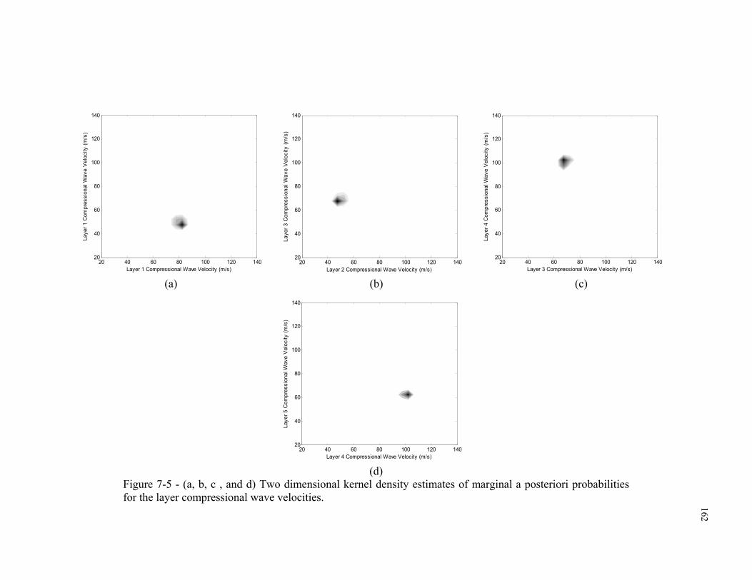
162

Layer 1 Compressional Wave Velocity (m/s)

Laye

r 1 C

ompr

essi

onal

Wav

e V

eloc

ity (m

/s)

20 40 60 80 100 120 14020

40

60

80

100

120

140

Layer 2 Compressional Wave Velocity (m/s)

Laye

r 3 C

ompr

essi

onal

Wav

e V

eloc

ity (m

/s)

20 40 60 80 100 120 14020

40

60

80

100

120

140

Layer 3 Compressional Wave Velocity (m/s)

Laye

r 4 C

ompr

essi

onal

Wav

e V

eloc

ity (m

/s)

20 40 60 80 100 120 14020

40

60

80

100

120

140

(a) (b) (c)

Layer 4 Compressional Wave Velocity (m/s)

Laye

r 5 C

ompr

essi

onal

Wav

e V

eloc

ity (m

/s)

20 40 60 80 100 120 14020

40

60

80

100

120

140

(d)

Figure 7-5 - (a, b, c , and d) Two dimensional kernel density estimates of marginal a posteriori probabilities for the layer compressional wave velocities.

163

Experimental Waveforms

The test results used in this section were collected as a part of the SPA testing and

monitoring performed in the course of a research project on investigation of the pavement

material characterization and its seasonal variation conducted jointly by Rutgers

University and Stantec Inc. The details of the project and its results have been published

in a number of reports and papers [Zaghloul et al. 2006].

For the example considered here, acceleration time histories A1, A2 and A3 from

a test on a flexible pavement section were considered as the experimental data. While, the

device collects much more information than these three time records, only these three

accelerometers were considered to illustrate the potential of the waveform inversion

technique.

SPA is originally designed to record the changes in acceleration and load in terms

of raw analog to digital (A/D) counts and not in terms of actual acceleration and load

values. The A/D counts are adequate for implementation of the aforementioned five

seismic techniques. Typical acceleration records collected during a test on a flexible

pavement, along with the inducing loading wavelet of high frequency hammer measured

by the load cell mounted on the hammer, are presented in Figure 7-7 in terms of A/D

counts. The translation of these records from the A/D counts to the actual acceleration

and load values requires multiplication of the recorded histories by calibration factors,

which were not available for this study. However, as will be illustrated below, this step is

not necessary for the waveform inversion application presented here.

By inspection of the data in Figure 7-7, it can be observed that the recorded

waveforms contain an initial wave packet followed by other oscillations. Intuitively, the

164

initial packet of the waves at each receiver location, which generally occurs between 0

and 0.001 seconds, contains the major portion of the information carried by the waves.

Therefore, for the example presented here, this portion of the wave is windowed using a

Hamming window [Oppenheim and Schafer 1989] and resulting waveforms are

considered as input data in the inversion procedure. The windowing functions along with

the windowed waveforms are depicted in Figure 7-8.

165

0 0.5 1 1.5 2 2.5 3 3.5 4

x 10-3

-1500

-1000

-500

0

500

1000

1500

Accelerometer A1

Time(sec)

A/D

Cou

nt

0 0.5 1 1.5 2 2.5 3 3.5 4

x 10-3

-1500

-1000

-500

0

500

1000

1500

Accelerometer A2

Time(sec)

A/D

Cou

nt

0 0.5 1 1.5 2 2.5 3 3.5 4

x 10-3

-1500

-1000

-500

0

500

1000

1500

2000

Accelerometer A3

Time(sec)

A/D

Cou

nt

0 0.5 1 1.5 2 2.5 3 3.5 4

x 10-3

-200

0

200

400

600

800

Time (Sec)

A/D

Cou

nt

Load

Figure 7-7 –A/D counts from accelerometers A1, A2, A3, and the high frequency hammer from a test on a flexible section.

166

0 0.5 1 1.5 2 2.5 3 3.5 4

x 10-3

0

0.2

0.4

0.6

0.8

1

Time(sec)

Win

dow

Hamming Window

0 0.5 1 1.5 2 2.5 3 3.5 4

x 10-3

-600

-400

-200

0

200

400

600

800

Acceleration A1

Time(sec)

A/D

Cou

nt

0 0.5 1 1.5 2 2.5 3 3.5 4

x 10-3

-1000

-500

0

500

1000

1500

Acceleration A2

Time(sec)

A/D

Cou

nt

0 0.5 1 1.5 2 2.5 3 3.5 4

x 10-3

-1500

-1000

-500

0

500

1000

1500

Accelerometer A3

Time(sec)

A/D

Cou

nt

Figure 7-8 – Hamming window function and A/D counts from accelerometers A1, A2, A3 after the windowing operation.

Accelerometer

Accelerometer

167

Forward Model

To evaluate the response of a pavement section to various loads, pavements are

generally modeled as horizontally layered systems. Due to a low intensity of the

excitation in the SPA test, the response of the pavement is essentially a linearly elastic

one. Therefore, a spectral element model, as presented in Appendix A, can be used as a

representative model and is considered here as the forward model.

To predict the theoretical response of a typical pavement section during a SPA

test, the recorded A/D counts of the loading time history, as presented in Figure 7-7, is

used as an input to the model. The resulting waveforms are then windowed using the

same windowing operations as described earlier. It should be noted that, since the input

loading history is given and used in terms of A/D counts, the magnitude of the predicted

accelerations from the model can not be realistic. However, since the pavement system is

essentially linearly elastic, the relative variation of the acceleration is realistic and can be

compared to the relative variation of acceleration in actual recorded data. To perform

such a comparison during the inversion, the predicted acceleration time history at each

receiver location is scaled so that the value of its maximum matches the value of the

maximum acceleration in the actual data. Once this scaling has been performed, the

theoretical and experimental data are compared to each other.

Results of Inversion of SPA Data

Using the presented forward model, the SPA data was analyzed to obtain the layer

elastic modulus and layer thickness for each layer. For this analysis, the pavement was

168

modeled as a three layer system; an asphalt layer over a base layer, underlain by an

infinite subgrade layer. The combined data and modeling uncertainty covariance was

selected to be one unit of A/D count. Obviously, a more comprehensive analysis is

required to identify an appropriate value for modeling and data uncertainties. However, in

this analysis, a nominal uncertainty value was selected to illustrate the waveform

inversion for experimental test data. Kernel density estimates of marginal a posteriori

probability densities for the layer moduli obtained from the probabilistic backcalculation

are presented in Figure 7-9. A comparison of the acceleration time histories for the

pavement section with the most probable layer moduli and the observed data are

presented in Figure 7-10. It can be observed that the waveform inversion has identified

the layer moduli and thicknesses. However, the uncertainty of the moduli is much lower

than the uncertainty of the thicknesses calculated from the inversion analysis. It should be

mentioned that the objective of the presented analysis was to validate the applicability of

the waveform inversion for experimental data. Although the presented results validate the

applicability of the approach, further research is required to completely understand

different aspects of the waveform inversion for shallow subsurface investigation. The

research should try to address a number of issues, such as evaluation of uncertainties in

the modeling by comparing actual and theoretical data and verifying the inversion

analysis by comparison of the results to other reference data such as laboratory test

results. Such reference data were not available for this preliminary study.

169

0.1 0.2 0.3 0.4 0.5Paving Layer Thickness (m)

Mar

gina

l Pro

babi

lity

0.1 0.2 0.3 0.4 0.5Base Layer Thickness (m)

Mar

gina

l Pro

babi

lity

(a) (b)

1.3 1.32 1.34 1.36 1.38 1.4

x 1010Asphlat Layer Modulus (Pa)

Mar

gina

l Pro

babi

lity

1.1 1.15 1.2 1.25 1.3

x 109

0

Base Layer Modulus (Pa)

Mar

gina

l Pro

babi

lity

0.9 0.95 1 1.05 1.1

x 109Subgrade Modulus (Pa)

Mar

gina

l Pro

babi

lity

(c) (d) (e)

Figure 7-9 – - Kernel density estimates of marginal a posteriori probabilities for the layer thickness (a and b) and layer moduli (c, d, and e) obtained from the probabilistic inversion of the acceleration time histories.

170

0 0.5 1 1.5 2 2.5 3 3.5 4

x 10-3

-600

-400

-200

0

200

400

600

800

Accelerometer A1

Time(sec)

A/D

Cou

nt

ObservedCalculated

0 0.5 1 1.5 2 2.5 3 3.5 4

x 10-3

-1000

-500

0

500

1000

1500

Accelerometer A2

Time(sec)

A/D

Cou

nt

ObservedCalculated

0 0.5 1 1.5 2 2.5 3 3.5 4

x 10-3

-1500

-1000

-500

0

500

1000

1500

Accelerometer A3

Time(sec)

A/D

Cou

nt

ObservedCalculated

Figure 7-10 – Comparison of the acceleration time histories for the pavement section with the most probable layer moduli and the observed data.

171

Summary The probabilistic formulation of the seismic waveform inversion problem for

evaluation of subsurface properties in civil engineering was presented in this chapter.

Using a set of synthetic data, the potential of the waveform inversion for evaluation of the

subsurface profiles was illustrated. It was shown that the waveform inversion is a

powerful technique, which is not limited by many of the assumption of other seismic

techniques such as Spectral Analysis of Surface Waves (SASW). Finally, by inversion of

a set of experimental seismic data collected for a pavement section by Seismic Pavement

Analyzer (SPA), the feasibility of the application of the probabilistic waveform inversion

approach to real data was illustrated.

References ABAQUS (2005), Hibbitt, Karlsson, and Sorensen, Providence, RI. Gucunski, N., and Woods, R. D. (1991), “Instrumentation for SASW Testing.”

Geotechnical Special Publication No. 29, Recent Advances in Instrumentation, Data Acquisition, and Testing in Soil Dynamics, New York: American Society of Civil Engineers, pp. 1-16.

Nazarian, S., Stokoe, K.H., II and Hudson, W.R. (1983), "Use of Spectral Analysis of Surface Waves Method for Determination of Moduli and Thicknesses of Pavement Systems," Transportation Research Record, No. 930, National Research Council, Washington, D.C., 38-45.

Nazarian, S. (1984), “In situ determination of elastic moduli of soil deposits and pavement systems by spectral analysis of surface waves method” PhD thesis, Univ. of Texas at Austin, Texas.

Nazarian S., Baker M.R. and Crain K. (1993), “Development and Testing of a Seismic Pavement Analyzer - Software and Hardware” Report SHRP-H-375, Strategic Highway Research Program, National Research Council, Washington, D.C.

Oppenheim, A.V., and Schafer R.W., (1989), “Discrete-Time Signal Processing”, Prentice-Hall.

Park., C.B., Miller, R. D., and Xia, J. (1999), “Multichannel Analysis of Surface Waves” Geophysics, Vol. 64, No. 3, pp. 800-808.

Priestly (1981) “Spectral Analysis of Time Series”, Academic Press, New York. Reddy, S. (1992), “Improved Impulse Response Testing - Theoretical and Practical

Validations” M.S. Thesis, The University of Texas at El Paso.

172

Sansalone, M, (1997), “Impact-Echo: The Complete Story” ACI Structural Journal, Vo. 94, No. 6, pp. 777-786.

Zaghloul, S.M., Gucunski, N., Jackson, H., and Hadidi, R. (2006), “Material Characterization and Seasonal Variation in Material Properties”, Report No. FHWA-NJ-2005-024, New Jersey Department of Transportation, Trenton, NJ.

173

8 Closure

Summary and Conclusions In this dissertation, a general probabilistic approach to the solution of the inverse

problems was introduced as a better approach to the solution of inverse problems. The

mathematical framework required for implementation of this approach was presented in

detail. This approach is a new approach to inverse problems in civil engineering and is

different from the currently used deterministic approach, where the objective is to find

the model of a system, for which the theoretical response best fits the observed data.

Following the mathematical formulation of the approach, techniques for direct analytical

evaluation and numerical approximation of the probabilistic solution using Monte Carlo

Markov Chains (MCMC), with and without Neighborhood Algorithm (NA)

approximation, were introduced and explained. The application of the presented concepts

and techniques was then illustrated in practical terms using a simple modulus

determination experiment.

The probabilistic approach was applied to three important classes of inverse

problems in geotechnical/transportation engineering as application examples. These

applications were:

174

• Pavement modulus backcalculation for Falling Weight Deflectometer (FWD),

• Model calibration based on geotechnical instrument measurements, and

• Seismic waveform inversion for shallow subsurface characterization.

A brief summary of the major findings in each application is presented below.

FWD Backcalculation

As the first application, probabilistic FWD backcalculation was introduced

formulated, and the results of the backcalculation of synthetic test data were presented.

The probabilistic backcalculation was then used as a tool to compare different

backcalculation procedures, such as static and dynamic backcalculation procedures.

Based on the presented results, it was shown that the static backcalculation procedures

fail to capture the essential dynamic nature of the test and consequently can not be relied

upon for accurate backcalculation. It was also demonstrated that there is little redundancy

in dynamic deflection bowl backcalculation procedures, which can produce large

uncertainties in obtained backcalculation results. Among the compared backcalculation

procedures, the dynamic deflection time history backcalculation offers the best and most

reliable approach in the FWD backcalculation. The application of this approach was then

illustrated both on synthetic and actual experimental data. It was also shown that, at least

in the case of synthetic data, the deflection time histories carry enough information to

simultaneously backcalculate for layer moduli and bedrock depth. Finally, the effect of

frequency dependent layer material properties on predicted deflection time histories was

175

investigated. It was shown that such effects can be significant and produce discrepancies

in the backcalculation results.

Model Calibration

As the second application, calibration of a finite element settlement prediction

model for a landfill redevelopment project was presented. This example demonstrated

how the probabilistic inversion approach can be used to complement the application of

the observational method in geotechnical engineering. The basic formulation of the

probabilistic solution was described for this problem and the calibration of a settlement

prediction model using the probabilistic approach was then outlined and the results of the

analysis were presented. It was illustrated that the ability of the probabilistic approach to

evaluate the uncertainties of the obtained results provides an engineer with very valuable

information regarding the limitations of the data and results. Consequently, it enables

him/her to devise an appropriate course of action.

Seismic Inversion

As the last application, the probabilistic formulation of a seismic waveform

inversion problem for evaluation of shallow subsurface properties was presented. Using a

set of synthetic data, the potential of the waveform inversion for evaluation of the

subsurface profiles were illustrated. It was shown that the waveform inversion is a

powerful technique, which is not limited by many of the assumption of other seismic

techniques, such as Spectral Analysis of Surface Waves (SASW). Finally, the feasibility

176

of the application of the probabilistic waveform inversion approach to real data was

illustrated by inversion of a set of experimental seismic data collected for a pavement

section by Seismic Pavement Analyzer (SPA).

Recommendations for Future Research The following are recommendations for further development of the probabilistic

approach and its adoption in engineering practice:

• The probabilistic approach to the solution of inverse problems is a

mathematical tool that can be applied to virtually any inverse problem in civil

engineering. Advantages of using the probabilistic approach in other civil

engineering applications should be further explored.

• To introduce the approach in this research, Matlab® was used as a

development environment and generic computer codes were generated for

application of the approach. However, to optimize the computational

efficiency of the approach and facilitate its implementation, development of

efficient stand alone and application oriented codes should be considered.

• One essential component of any inverse problem is the forward model used in

generation of the theoretical solution. Development of efficient forward

models for each application and evaluation of their uncertainties in

comparison to actual measurements will be an essential and necessary next

step in further development of the presented approach.

177

• As outlined in this research, in probabilistic approach, the input parameters of

an inverse problem should be accompanied by uncertainty measures

represented by a priori information. There limited guidelines in literature

addressing the uncertainties in different contexts. A comprehensive review of

these guidelines for application in probabilistic approach is required. This

review should be followed by development of application oriented guidelines

to facilitate the application of this approach as a practical tool.

178

Appendix A: Spectral Element Method for Analysis of Wave Propagation in Layered Media

Introduction Finite element method is a general and accepted numerical tool in analysis of

wave propagation. However, in spite of the recent advances in computational capabilities,

significant resources are still required to perform a reasonably accurate wave propagation

analysis using finite element method. In the finite element analysis, the number and type

of elements control the computational time required to solve the model. The number of

elements required to converge a dynamic finite element model is generally more than a

static model and tend to increases with increased excitation frequency. For a structure

analyzed at a high excitation frequency, the number of elements may easily exceed the

practical number to solve the problem in a timely manner.

For horizontally layered media, over the years, a series of more efficient

techniques have been developed, which involves a combination of analytical and

numerical solutions. The general similarity of these techniques, referred to here as

frequency domain techniques, is that the solution is obtained by a synthesis of waveforms

179

from superposition of many frequency components, which are in part are obtained

analytically. The most notable work in this area has been done by Thomson [1950] and

Haskell [1953], who developed the layer transfer matrix method. In this method, for a

given layer, the amplitude of displacement and force vector at one interface are related to

the amplitude of displacement and force at the other interface for each frequency

component through the transfer matrix. Kausel and Roesset [1981] further developed this

technique by introducing a layer stiffness matrix similar to those in the finite element

method. The transfer and stiffness matrices involve transcendental functions which

exhibit numerical complications in implementations.

To overcome this problem, a semi discrete solution was introduced by Lysmer

[1970] and was further generalized by Kausel and Roesset [1981]. The basic idea of this

solution is to divide layers into sublayers with thicknesses shorter than the wavelength of

interest and to approximate the wave in the vertical direction by a linear interpolation

between layer interfaces, assuming that the mass of each layer is lumped at the interfaces.

By doing so, the transcendental equation will be replaced by a simple eigenvalue

problem, which can be solved by standard techniques.

The requirement of subdivision of layers to sublayers of small thickness results in

a large system of equations that should to be solved for each frequency component. This

makes these techniques rather computationally expensive. The spectral element method

[Rizzi and Doyle, 1992, Doyle, 1997] overcomes this issue by modeling the exact mass

distribution and using double summation over significant wave numbers and frequencies

instead of numerical integration. Consequently, each layer is modeled exactly without the

need to subdivide the layer. Hence the method becomes more efficient.

180

The spectral element method can be described as a variation of p-type

convergence analysis in finite element. In dynamic finite element analysis the

convergence can be obtained by either increasing the number of elements or increasing

the polynomial order of the interpolation functions. If the convergence is obtained by

increasing the order of the interpolating function, the convergence is generally referred to

as p-type convergence. Typically, the order of the polynomial interpolation function is

increased, while the spatial mesh is held constant, until more accurate results are

obtained. In spectral elements, the element interpolation functions are based on the

eigenfunctions of the differential equation used to represent the dominant mechanics in

the problem. This results in the “exact” form of the displacement field for the

interpolation function. The interpolation functions of spectral elements are based on

trigonometric functions, opposed to polynomial functions of conventional elements. The

trigonometric functions incorporate the frequency of the response into the interpolation

function. Having the interpolation function based on the eigenfunctions means that a

single spectral element will give the “exact” dynamic solution across the element for

simple loading and boundary conditions. This results in a reduced number of elements,

and thus a reduced model size for a spectral element model as compared to the

conventional finite element model.

This appendix provides the basic formulation of the spectral elements and

describes its implementation in this research. This appendix is not intended to be a

tutorial about this technique. Further details of derivation and implementation of this

approach can be found in cited references.

181

Spectral Wave Analysis The general form of spectral element analysis approach to wave propagation is

presented by Doyle [1997]. This approach is illustrated here for the wave propagation

analysis in an axi-symmetric horizontally layered media [Alkhoury et. al 2001].

The general equation of motion for an isotropic elastic material can be represented

by the following coupled differential equation:

UUU ρµµλ =∇+∇∇+ 2.)( (A-1) where U is the displacement vector, ρ is the material density, µ and λ are the Lame

constants, ∇ is the vector differential operator, ⋅∇ is the divergence operation and, 2∇ is

the vector Laplacian operation.

Using Helmholtz decomposition [Achenbach, 1973], the displacement field can

be expressed in terms of gradient of a scalar potential function ϕ and the curl of a vector

potential functionψ as:

ψϕ ×∇+∇=u (A-2) For an axi-symmetric motion, the vector potential ψ has only one component θψ .

Denoting the displacements in r and z direction by u and w the displacements and

potentials are related by:

zru

∂∂

−∂∂

= θψϕ

rr

rzw

∂∂

+∂∂

=)(1 θψϕ

(A-3)

and stress-displacement relationships are given by:

rru

rzw

zz ∂∂

+∂∂

+=)()2( λµλσ

)(

rw

zu

zr ∂∂

+∂∂

= µτ

(A-4)

These potentials can be obtained by solution of the following differential

equations, which are a set of decoupled equations obtained by substitution of Equation

(A-3) into Equation (A-1).

182

2

2

22

2

2

2 11tczrrr p ∂

∂=

∂∂

+∂∂

+∂∂ ϕϕϕϕ

2

2

222

2

2

2 11tcrzrrr s ∂

∂=−

∂∂

+∂

∂+

∂∂ θθθθθ ψψψψψ

(A-4)

where pc and sc are compressional and shear wave velocities of the medium defined

respectively as 2/1)2(ρ

µλ +=pc and 2/1)(

ρµ

=sc .

These equations can be transformed to the frequency domain using the Fourier

transform:

ϕωϕϕϕ ˆ1ˆˆ1ˆ 222

2

2

2

pczrrr=

∂∂

+∂∂

+∂∂

θθθθθ ψω

ψψψψ ˆ1ˆˆˆ1ˆ 2222

2

2

2

scrzrrr=−

∂∂

+∂

∂+

∂∂

(A-5)

where hat sign indicates that the expression is in the frequency domain and ω is the

frequency. These equations can be solved by separation of variables.

To discretize the solution, a boundary condition is imposed on the problem.

Assuming that at the radial boundary Rr = (far from load) the amplitude of oscillations

vanishes, the generic solution of wave equation can be discretized and is given by double

summation over discrete angular frequency nω with Nn ,...,1= and discrete wave

number R

k mm

α= with Mm ,...,1= , where mα is the m th positive root of Bessel

function of first kind , 0J . The solution is presented below:

∑∑ −−=n m

tim

zikmn

npzmn erkJeA ωϕ )(0

∑∑ −−=n m

tim

zikmn

nszmn erkJeB ωθψ )(1

(A-6)

183

where 1J is the Bessel function of first kind and order one, mnA and mnB are coefficients

to be determined from the boundary conditions and szmnk and pzmnk satisfy the following

relations referred to as spectrum relations:

2/122

2

)( mp

npzmn k

ck −=

ω

2/12

2

2

)( ms

nszmn k

ck −=

ω

(A-7)

Spectral Element Formulation The obtained discretized solution can be used to derive the spectral elements

formulation. Such a derivation is presented below for a two node layer element and a one

node half space element.

Two-Node Layer Element

The two node layer element with a height of h , which is depicted in Figure A-1,

can be visualized as a layer confined by two circular surfaces within which the wave is

constrained to move. The response at any point in the element is determined by a

superposition of incident and reflected waves from each surface. To include both incident

and reflected waves, the following general solution that is obtained by adding two

potentials is considered. These potentials include waves propagating in both directions:

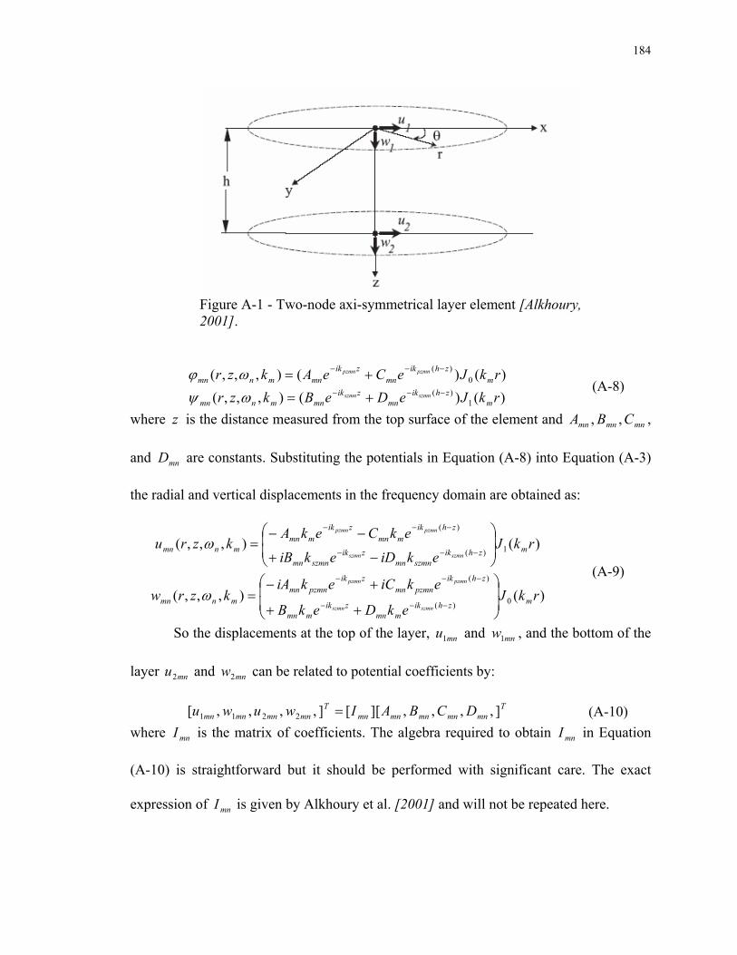
184

Figure A-1 - Two-node axi-symmetrical layer element [Alkhoury, 2001].

)()(),,,( 0)( rkJeCeAkzr m

zhikmn

zikmnmnmn

pzmnpzmn −−− +=ωϕ )()(),,,( 1

)( rkJeDeBkzr mzhik

mnzik

mnmnmnszmnszmn −−− +=ωψ

(A-8)

where z is the distance measured from the top surface of the element and mnA , mnB , mnC ,

and mnD are constants. Substituting the potentials in Equation (A-8) into Equation (A-3)

the radial and vertical displacements in the frequency domain are obtained as:

)(),,,( 1)(

)(

rkJekiDekiB

ekCekAkzru mzhik

szmnmnzik

szmnmn

zhikmmn

zikmmn

mnmnszmnszmn

pzmnpzmn

⎟⎟⎠

⎞⎜⎜⎝

⎛

−+

−−=

−−−

−−−

ω

)(),,,( 0)(

)(

rkJekDekB

ekiCekiAkzrw mzhik

mmnzik

mmn

zhikpzmnmn

zikpzmnmn

mnmnszmnszmn

pzmnpzmn

⎟⎟

⎠

⎞

⎜⎜

⎝

⎛

++

+−=

−−−

−−−

ω

(A-9)

So the displacements at the top of the layer, mnu1 and mnw1 , and the bottom of the

layer mnu2 and mnw2 can be related to potential coefficients by:

Tmnmnmnmnmn

Tmnmnmnmn DCBAIwuwu ],,,,][[],,,,[ 2211 = (A-10)

where mnI is the matrix of coefficients. The algebra required to obtain mnI in Equation

(A-10) is straightforward but it should be performed with significant care. The exact

expression of mnI is given by Alkhoury et al. [2001] and will not be repeated here.

185

Similar to the derivation of Equation (A-10), the surface traction kT at each

interface can be related to the potential coefficients using equations (A-4) and (A-9). To

obtain the surface tractions the Cauchy stress principle, mkmk nT τ= , is used. In this

equation, mn represents the normal to the surface of the layer and kmτ is the component

of the stress tensor. So the traction at the top of the layer, mnrT 1 and mnzT 1 , and the bottom

of the layer mnrT 2 and mnzT 2 , can be related to potential coefficients by:

Tmnmnmnmnmn

Tmnzmnrmnzmnr DCBAHTTTT ],,,,][[],,,,,,,[ 2211 = (A-11)

The exact expression of mnH is also given by Alkhoury et. al. [2001] and will not

be repeated here. Upon performing the required algebra to eliminate the coefficient from

equations (A-10) and (A-11), the tractions and displacements can be related to each other

by a complex and symmetric 4x4 dynamic stiffness matrix.

Tmnmnmnmnmn

Tmnzmnrmnzmnr wuwukTTTT ],,,,][[],,,,,,,[ 22112211 = (A-12)

where:

⎥⎥⎥⎥

⎦

⎤

⎢⎢⎢⎢

⎣

⎡

−−

=

mn

mnmn

mnmnmn

mnmnmnmn

mn

ksymkk

kkkkkkk

k

22

1111

244122

41312111

][ (A-13)

and

)})(({ 22112112222

11 QQkkQQkkkikk pzmnszmnmmszmnpzmnmn

mn ++∆

=µ

⎪⎭

⎪⎬⎫

⎪⎩

⎪⎨⎧

−−−

−−−+−

∆=

)2(

)exp(4)(3(22422

2111

221222

12szmnpzmnmszmnmm

szmnpzmnmszmnpzmnszmnm

mnmn kkkkkQQk

hikhikQQkkkkkk µ

)})exp()exp()((2{ 1121222

13 QhikkkQhikkkkikk szmnpzmnszmnpzmnmmszmnpzmnmn

mn −+−+−∆

=µ

186

)})exp())(exp((2{ 122222

14 QhikQhikkkkkk szmnpzmnmszmnszmnpzmnmn

mn −−−+∆

=µ

)})(({ 21122211222

22 QQkkQQkkkikk pzmnszmnmmszmnszmnmn

mn ++∆

=µ

)})exp()exp()((2{ 2111222

24 QhikkkQhikkkkikk pzmnpzmnszmnszmnmmszmnszmnmn

mn −+−+−∆

=µ

In which:

2111422

22122 )())exp(4(2 QQkkkQQhikhikkkk mszmnpzmnszmnpzmnszmnpzmnmmn +−−−−=∆

)2exp(111 hikQ pzmn−−=

)2exp(121 hikQ szmn−−=

)2exp(112 hikQ pzmn−+=

)2exp(122 hikQ szmn−+=

One-Node Half Space Element

In a one node half space element waves travel only in one direction. So only the

incident wave potential is considered in the derivation of the element matrix. An

illustration of the one node half space element is presented in Figure A-2. The steps in the

derivation of the stiffness matrix in this case are similar to the steps in the derivation of

the two node element presented earlier. Similar to the derivation for the two node

element, the stiffness matrix can be obtained as:

Tmnmnmn

Tmnzmnr wukTT ],][[],[ 1111 = (A-14)

where:

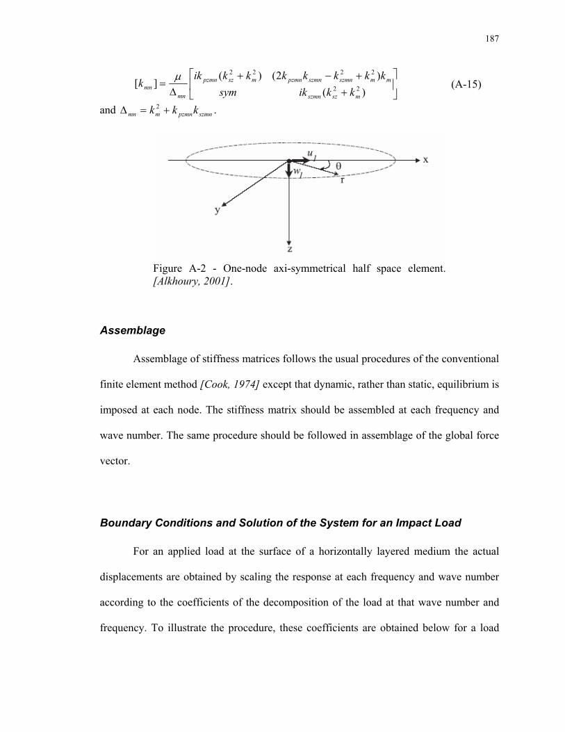
187

⎥⎦

⎤⎢⎣

⎡

++−+

∆=

)()2()(

][ 22

2222

mszszmn

mmszmnszmnpzmnmszpzmn

mnmn kkiksym

kkkkkkkikk µ (A-15)

and szmnpzmnmmn kkk +=∆ 2 .

Figure A-2 - One-node axi-symmetrical half space element. [Alkhoury, 2001].

Assemblage

Assemblage of stiffness matrices follows the usual procedures of the conventional

finite element method [Cook, 1974] except that dynamic, rather than static, equilibrium is

imposed at each node. The stiffness matrix should be assembled at each frequency and

wave number. The same procedure should be followed in assemblage of the global force

vector.

Boundary Conditions and Solution of the System for an Impact Load

For an applied load at the surface of a horizontally layered medium the actual

displacements are obtained by scaling the response at each frequency and wave number

according to the coefficients of the decomposition of the load at that wave number and

frequency. To illustrate the procedure, these coefficients are obtained below for a load

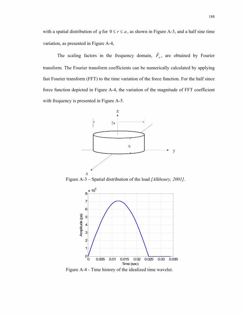
188

with a spatial distribution of q for ar ≤≤0 , as shown in Figure A-3, and a half sine time

variation, as presented in Figure A-4,

The scaling factors in the frequency domain, nF , are obtained by Fourier

transform. The Fourier transform coefficients can be numerically calculated by applying

fast Fourier transform (FFT) to the time variation of the force function. For the half since

force function depicted in Figure A-4, the variation of the magnitude of FFT coefficient

with frequency is presented in Figure A-5.

Figure A-3 – Spatial distribution of the load [Alkhoury, 2001].

0 0.005 0.01 0.015 0.02 0.025 0.03 0.0350

1

2

3

4

5

6

7

8x 105

Time (sec)

Am

plitu

de (p

a)

Figure A-4 - Time history of the idealized time wavelet.

189

0 50 100 150 200 2500

2

4

6

8

10

12x 106

Frequency (Hz)

Am

plitu

de (P

a)

Figure A-5 - Frequency spectrum of the idealized wavelet.

The scaling factors in the wave number domain can be obtained based on Fourier-

Bessel theory. For a cylindrical shaped load of a radius a , the Fourier-Bessel coefficients

are given by [Kreyszig, 1999]:

)()(

2ˆ12

1

aR

JRJ

aF m

mmm

ααα

= Mm ,...,1= (A-16)

where mF is the coefficient of Fourier Bessel series for a wave number R

k mm

α= with

Mm ,...,1= , and mα is the m th positive root of the Bessel function of first kind , 0J .

The variation of Fourier-Bessel series coefficients for a circular load of a radius a , as

depicted in Figure A-3, is presented in Figure A-6.

190

Figure A-6 – Coefficients of Fourier-Bessel series for a circular load of a radius ma 15.0= .

Numerical Implementation The flowchart of the algorithm for implementation of the spectral element method

is presented in Figure A-7 [Alkhory et. al. 2001]. A Mathlab® code was developed based

on this algorithm to implement the presented spectral element approach. The algorithm

can be generally described by the following steps:

• Obtain time and wave number domain scaling factors by FFT and Fourier-

Bessel transform of the load function, respectively.

• Form the stiffness matrix of the system for each frequency and wave number.

• Solve for the displacements for a unit load in the frequency-wave number

domain for each frequency and wave number combination.

• Scale the calculated response using the obtained scaling factors.

• Sum all the wave number domain responses for each frequency to obtain the

response in the frequency domain.

191

• Use inverse FFT to obtain the response in the time domain.

Illustrative Example To verify the accuracy of the developed spectral element code, a numerical

example is considered and the results of the example are presented. The example

considered here is the simulation of the pavement response during the Falling Weight

Deflectometer (FWD) test. The pavement layer properties used for the numerical

simulation are presented in Table A-1. The spatial and time variation of the load function

considered for this example is similar to those presented in previous section.

The predicted surface deflection time histories by the spectral element method are

presented in Figure A-7. The response of the same pavement, as calculated by Alkhoury

[2001a], is presented in Figure A-8. These results are in very good agreement, which

confirms the accuracy of the developed code. Furthermore, as presented in Chapter 5,

these results are also in good agreement with finite element results.

Table A- 1 – Geometrical and material properties used in the numerical evaluation and verification of the spectral element method [Alkhoury, 2001].

Material Type Thickness (m)

Elastic Modulus (MPa)

Poisson’s Ratio

Mass Density (kg/m3)

Asphalt Concrete 0.15 1000 0.35 2300 Aggregate Base Course 0.25 200 0.35 2000

Subgrade infinity 100 0.35 1500

192

0 0.0125 0.025 0.0375 0.05-0.75

-0.6

-0.45

-0.3

-0.15

0

0.15

Time (sec)

Def

lect

ion

(mm

)

r= 0 mmr= 300 mmr= 600 mmr= 900 mmr=1200 mmr=1500 mm

Figure A-7 - Predicted pavement surface deflection time histories from the spectral element analysis.

Figure A-8 - Predicted pavement surface deflection time histories from the spectral element analysis [Alkhoury et al.,2001].

Summary In this appendix, derivation and implementation of the spectral elements

technique is presented. Spectral element method, is a frequency domain analysis

193

technique for horizontally layered media, such as pavements. The method is much more

efficient than the traditional finite element technique. The background and basic

formulation of the spectral element method was presented in this appendix and its

implementation was illustrated by the simulation of the FWD test. It is shown that the

results of the developed Mathlab® code are in agreement with results published by

others.

References Achenbach, J. D. (1973), “Wave Propagation in Elastic Solids”, Elsevier,

Amsterdam, Netherlands. Al-khoury, R., Scarpas, A., Kasbergen, C., Blaauwendraad, J. (2001a), “Spectral

Element Technique for Efficient Parameter Identification of Layered Media: Part I: Forward Model”, International Journal of Solids and Structures, Vol. 38.

Al-khoury, R., Scarpas, A., Kasbergen, C., Blaauwendraad, J. (2001b), “Spectral Element Technique for Efficient Parameter Identification of Layered Media: Part II: Inverse Calculations”, International Journal of Solids and Structures, Vol. 38.

Cook, R. D., (1974), “Concepts and Application of Finite Element Analysis”, Jon Wily and Sons, New York, NY.

Doyle, J.M. (1997), “Wave Propagation in Structures”, Springer-Verlag, NY. Haskell, N.A. (1953), “The Dispersion of Surface Waves on Multilayered Media”,

Bulletin of Seismological Society of America, Vol. 43, 17-34. Kausel, E. and Rosset, J. M. (1981), “Stiffness Matrices for Layered Soils”, Bulletin

of Seismological Society of America, Vol. 71, 1743-1761. Kreyszig, E. (1999), “Advanced Engineering Mathematics”, 8th. Edition, John Wiley

and Sons, New York, NY. Lysmer, J., (1970), “Lumped Mass Method for Rayleigh Waves”, Bulletin of

Seismological Society of America, V.60, No. 1, pp. 89-104. Rizzi, S.A. and Doyle, J.F. (1992), “Spectral Analysis of Wave Motion in Plane

Solids with Boundaries”, Trans. of ASME, Journal of Vibration and Acoustics, Vol 114, No. 2, pp. 133-140.

Thomson, W.T., (1950), “Transmission of Elastic Waves through a Stratified Solid Media”, Journal of Applied Physics, Vol. 21, p. 89-93.

194

Curriculum Vitae

Rambod Hadidi Education:

Ph.D. Civil Engineering, Rutgers University, New Brunswick, NJ, May 2007 M.Sc. Civil Engineering, Rutgers University, New Brunswick, NJ, May 2003 B.Sc. Civil Engineering, Sharif University of Technology, Tehran, Iran, June 1999

Academic Experience:

University of Texas at El Paso, El Paso, TX Lecturer - August, 2006 to December 2006

Rutgers University, Piscataway, NJ - January, 2002 to July 2006 Graduate Research Assistant – Spring, 2002; Summer, 2002; Fall, 2002; Spring,

2003; and Summer 2004 Substitute Lecturer- Spring, 2006 Lecturer- Fall, 2003; Spring, 2004; Fall, 2004; and summer 2005 Graduate Teaching Assistant – Fall 2004

New Jersey Institute of Technology, Newark, NJ – September 1999 to December 2001 Graduate Research Assistant - Fall, 1999; Spring, 2000; and Fall, 2000

Professional Experience:

Paulus, Sokolowski and Sartor, LLC, Warren, NJ Consultant/Project Geotechnical Engineer - April, 2004 to January, 2007

Transportation Infrastructure Systems Inc., Skillman, NJ Project Engineer - January, 2003 to January 2004

Qods Niroo Consulting Engineers, Tehran, IRAN Project Engineer - June 1999 to September 1999

Publications:

Journal and Peer Reviewed Publications:

Hadidi, R. and Gucunski, N. “A Probabilistic Approach to Solution of Inverse Problems in Civil Engineering”, ASCE Journal of Computing in Civil Engineering, (Accepted for publication).

Hadidi, R., and Gucunski, N. “A Probabilistic Approach to Falling Weight

Deflectometer Backcalculation”, The 86th Transportation Research Board Annual Meeting, Washington, DC, 2007.

195

Gucunski, N., Hadidi, R., Zaghlouol, S., Maher, A., and Shokouhi, P.,“Seasonal and Temperature Adjustment Models of Pavement Properties from Seismic Nondestructive Evaluation”, Geotechnical Special publication - Proceedings of GeoShanghai International Conference, Shanghai, China June 6-8, 2006 (accepted for publication).

Gucunski, N., Zaghlouol, S., Maher, A., Hadidi, R., and Shokouhi, P., “Development

of Seasonal Variation Models of Pavement Properties Using Seismic Nondestructive Testing (NDT) Techniques”, Geotechnical Special Publication, Proceedings of Geo-Institute Congress – Geotechnical Engineering in Information Technology Age, Atlanta, Georgia, February 26 to March 1, 2006.

Hadidi, R. and Saadeghvaziri, M.A., “Transverse Cracking of Concrete Bridge

Decks: the State-of-the-Art”, ASCE Journal of Bridge Engineering, Volume 10, Number 5, September/October 2005, pp 503-510.

Saadeghvaziri, M.A. and Hadidi, R., “Transverse Cracking of Concrete Bridge

Decks: Effects of Design Factor”, ASCE Journal of Bridge Engineering, Volume 10, Number 5, September/October 2005, pp 511-519.

Hadidi, R., Saadeghvaziri, M.A., and Hsu, T.H. “A Practical Tool to Accurately

Estimate Tensile Stresses in Concrete Bridge Decks to Control Transverse Cracking”, ASCE Practice Periodical on Structural Design and Construction, Volume 8, Number 2, 2003, pp74-82.

Hadidi, R., and Saadeghvaziri, M.A., “State of the Art of Early Age Transverse

Cracking of Concrete Bridge Decks”, The 82nd Transportation Research Board Annual Meeting, Washington, DC, January 15, 2003.