© 2016 nikhil bhosale
TRANSCRIPT

TOTAL LAGRANGIAN FORMULATION FOR LARGE DEFORMATION MODELING USING UNIFORM BACKGROUND MESH
By
NIKHIL BHOSALE
A THESIS PRESENTED TO THE GRADUATE SCHOOL
OF THE UNIVERSITY OF FLORIDA IN PARTIAL FULFILLMENT OF THE REQUIREMENTS FOR THE DEGREE OF
MASTER OF SCIENCE
UNIVERSITY OF FLORIDA
2016

© 2016 Nikhil Bhosale

To my parents

4
ACKNOWLEDGMENTS
Firstly, I would like to express my sincere gratitude to my advisor, Dr. Ashok V.
Kumar, for the continuous support of my thesis and related research, for his patience,
motivation, and immense knowledge. His guidance helped me in all the time of research
and writing of this thesis. I could not have imagined having a better advisor and mentor
for my thesis study.
I would like to thank Dr. Bhavani Sankar for being a member of my supervisory
committee. It is my honor to have him in my committee and be guided for my thesis. I
am grateful for his willingness to review this thesis and provide valuable suggestions.
Last but not the least, I would like to thank my family: my parents and to my
brothers and sister for supporting me spiritually throughout writing this thesis and my life
in general.

5
TABLE OF CONTENTS page
ACKNOWLEDGMENTS .................................................................................................. 4
LIST OF TABLES ............................................................................................................ 7
LIST OF FIGURES .......................................................................................................... 8
LIST OF ABBREVIATIONS ........................................................................................... 10
ABSTRACT ................................................................................................................... 11
CHAPTER
1 INTRODUCTION .................................................................................................... 13
Overview ................................................................................................................. 13
Goals and Objectives .............................................................................................. 15 Goal .................................................................................................................. 15 Objectives ......................................................................................................... 15
Outline .................................................................................................................... 16
2 INTRODUCTION TO IMPLICIT BOUNDARY METHOD ......................................... 17
Solution Structure ................................................................................................... 17 Imposing Essential Boundary Conditions ................................................................ 19
Essential Boundary Function .................................................................................. 19 Boundary Value Function ........................................................................................ 21
3 NONLINEAR FINITE ELEMENT ANALYSIS .......................................................... 24
Basic Principle ........................................................................................................ 24 Principle of Virtual Work .......................................................................................... 24
Total Lagrangian Formulation ................................................................................. 26 Linearization ........................................................................................................... 27
The Residual 𝒓 ................................................................................................. 27 The Newton-Raphson Iteration ......................................................................... 28
Discretization .......................................................................................................... 29
4 IMPLICIT BOUNDARY METHOD FOR NONLINEAR ANALYSIS .......................... 33
Governing Equation for Nonlinear Analysis Using IBFEM ...................................... 33 Discretization Using IBFEM .................................................................................... 35 Constructing The Global Stiffness Matrix ................................................................ 36

6
5 RESULT AND DISCUSSION .................................................................................. 38
2D Examples .......................................................................................................... 38 Plane Stress: A Plate Subjected to Uniform Pressure at the Top ..................... 38
Plane Stress: Thin Frame-like Structure ........................................................... 41 Axisymmetric: Thin Disk ................................................................................... 43
3D Shell Example ................................................................................................... 46 Cantilever Subjected to End Shear Force ........................................................ 46
Application in Flexural Hinge Design ...................................................................... 48
6 CONCLUSION ........................................................................................................ 51
Summary ................................................................................................................ 51
Scope of Future Work ............................................................................................. 52
LIST OF REFERENCES ............................................................................................... 53
BIOGRAPHICAL SKETCH ............................................................................................ 55

7
LIST OF TABLES
Table page 5-1 Maximum deflection comparison. ....................................................................... 41
5-2 Maximum deflection comparison. ....................................................................... 43
5-3 Maximum deflection comparison. ....................................................................... 46
5-4 Vertical tip deflections for the cantilever loaded with end shear force. ............... 48

8
LIST OF FIGURES
Figure page 2-1 Representation of essential boundary and band in boundary element ............... 20
2-2 Boundary value function ..................................................................................... 22
3-1 Configuration at time 0, t and t t ................................................................... 25
3-2 Configuration at time 0, 𝑡 and 𝑡 + ∆𝑡 or 0, 𝑘 and 𝑘 + 1 iteration .......................... 28
5-1 A plane strain plate subjected to uniform pressure at the top ............................. 39
5-2 FE Model ............................................................................................................ 39
5-3 Displacement at P=100 ..................................................................................... 39
5-4 Stress along x-direction ..................................................................................... 40
5-5 Von-Mises Stress ............................................................................................... 40
5-6 Maximum Deflection vs Pressure 𝑃 . .................................................................. 41
5-7 Thin beam structure ............................................................................................ 42
5-8 Thin beam structure ........................................................................................... 42
5-9 Maximum Deflection vs Pressure 𝑃 ................................................................... 43
5-10 Thin Disk ............................................................................................................ 44
5-11 FE Model ............................................................................................................ 44
5-12 Displacement at P=100 ...................................................................................... 45
5-13 Von-Mises Stress .............................................................................................. 45
5-14 Maximum Deflection vs Pressure 𝑃 ................................................................... 45
5-15 Cantilever beam subjected to end shear load .................................................... 47
5-16 Cantilever beam model. ...................................................................................... 47
5-17 Deflection vs Load graph. ................................................................................... 47
5-18 Dimensions, Forces and coordinates of a flexural hinge .................................... 48
5-19 FE Model ............................................................................................................ 49
9
5-20 Maximum Displacement comparison .................................................................. 49
5-21 Von-mises stress contours ................................................................................. 50

10
LIST OF ABBREVIATIONS
3D Three Dimensions
EBC Essential Boundary Condition
FEM Finite Element Method
IBFEM Implicit Boundary Finite Element Method
NURBS Non-Uniform Rational B-Splines
X-FEM Extended Finite Element Method

11
Abstract of Thesis Presented to the Graduate School of the University of Florida in Partial Fulfillment of the Requirements for the Degree of Master of Science
TOTAL LAGRANGIAN FORMULATION FOR LARGE DEFORMATION MODELING USING UNIFORM BACKGROUND MESH
By
Nikhil Bhosale
May 2016
Chair: Ashok V. Kumar Major: Mechanical Engineering
The need for optimized structures, new materials and increased safety standards
has increased the demand of nonlinear analysis in recent years. The finite element
method is used to numerically compute stiffness and internal force matrices and the
corresponding iterative problem is solved using the modified Newton-Raphson method.
A typical finite element program to perform this analysis has three steps: a
representative finite element model, the analysis of the model and the interpretation of
results. A representative finite element model and the formulation of the applied
loads/boundary conditions are key factors for a reliable and accurate response
prediction of the model.
Implicit Boundary Method uses a uniform background mesh for the finite element
analysis and thus avoids the need for a conforming mesh. Mesh generation difficulties
can be avoided when a background mesh rather than a mesh that conforms to the
geometry is used for the analysis. The geometry is represented by equations and is
independent of the mesh and is immersed in the background mesh. The solution to
12
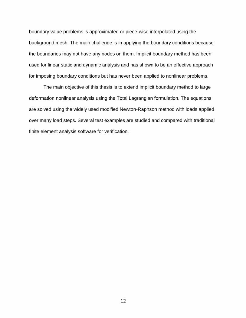
boundary value problems is approximated or piece-wise interpolated using the
background mesh. The main challenge is in applying the boundary conditions because
the boundaries may not have any nodes on them. Implicit boundary method has been
used for linear static and dynamic analysis and has shown to be an effective approach
for imposing boundary conditions but has never been applied to nonlinear problems.
The main objective of this thesis is to extend implicit boundary method to large
deformation nonlinear analysis using the Total Lagrangian formulation. The equations
are solved using the widely used modified Newton-Raphson method with loads applied
over many load steps. Several test examples are studied and compared with traditional
finite element analysis software for verification.

13
CHAPTER 1 INTRODUCTION
Overview
When the deformation of the structure is large compared with its original
configuration, the response is considered nonlinear due to geometric nonlinearity even if
the material behavior is still elastic. Such problems have been solved using two different
formulations: Total Lagrangian (TL) and Updated Lagrangian (UL). In the former
approach, the quantities of interest are mapped to the original undeformed configuration
in the principle of virtual work. In the UL formulation, the geometry is updated at the end
of each load step. As the geometry is in the undeformed configuration for the TL
formulation it is easier to implement and best suited for applications where the material
is elastic. Large deformation analysis is needed for slender structures used in
aerospace, civil and mechanical engineering applications. A variety of structures are
designed to be compliant so that they undergo large deformation to facilitate the
functioning of machinery and devices. In this thesis, we explore the possibility of using a
background mesh for the analysis to avoid the difficulties related to mesh generation.
The geometry is defined using equations of the boundaries and it is immersed in the
background mesh. The boundaries can pass through the elements due to which we
cannot assume that the nodes of the mesh are available at the boundaries for applying
boundary conditions. The implicit boundary method was developed to apply essential
boundary conditions on such boundaries and has been applied to a variety of linear
static and dynamic problems [1]-[5]. In the present work, we study how this method
could be extended to large deformation analysis.

14
The traditional FEM uses a conforming mesh that approximates the geometry
and provides the basis for piecewise interpolation of the field variables. But a
conforming mesh is often difficult to generate, especially for complex geometry. As a
result, many methods for avoiding mesh generation have been developed and other
modifications of the traditional finite element analysis have been developed that reduce
the difficulty associated with mesh generation. These include meshless methods,
isogeometric method, extended FEM and mesh independent methods that use a
background mesh. An extensive overview of several meshless or meshfree methods
can be found in several books and review papers such as Liu [6] and Gu [7]. Moving
Least Square (MLS) method [8], Element-Free Galerkin Method (EFGM) [9] and
Meshless Local Petrov-GalerKin Method [10] are examples of meshless methods. In the
meshless methods, as set of nodes scattered over the domain is used for the analysis
and these nodes are not connected to form elements. Meshless methods have also
been applied to structural dynamics [11]-[12]. Meshless methods use shape function
that do not need element connectivity but these shape functions are expensive to
evaluate as a result. The geometry is approximated by the nodes on the boundary so
applying boundary conditions is challenging and the basis functions used for meshless
approximation do not have Kronecker delta properties. As a result other methods that
are mesh independent such as XFEM have become more popular [13]. In XFEM the
geometry of defects, such as cracks, are modeled using equations rather than the mesh
itself so that the mesh does not have to be modified to simulate crack propagation.
In this thesis, we study a mesh independent approach where a background mesh
is used for the analysis. This method has been referred to as the Implicit Boundary

15
Finite Element Method (IBFEM) because we use the implicit boundary method to
impose essential boundary conditions. A structured uniform background mesh that
consists of regular shaped undistorted elements is used for interpolating or
approximating the solution. Using a mesh with undistorted elements improves the
quality of the solution by reducing numerical quadrature errors. Such a mesh is also
easy to generate because it does not have to fit within the geometry. The bounding box
within which the geometry fits is subdivided into uniform elements and then any element
that is complete outside the geometry is removed to obtain the final background mesh
for analysis. This process is easy to automate regardless of the complexity of the
geometry. Furthermore, the implicit boundary method can be used with basis functions
that do not satisfy Kronecker’s delta properties such as B-spline basis functions and
meshless shape functions. Elements that use quadratic and cubic B-splines have been
developed. Application to static problems such as elastic problems and heat conduction
problems have been demonstrated in past work, but the feasibility of using IBFEM for
non-linear analysis has not been studied. Motivated by this, we explore the use of
IBFEM for nonlinear analysis using Total lagrangian formulation.
Goals and Objectives
Goal
The main objective of this thesis is to extend the Implicit Boundary Finite Element
Method (IBFEM) to large displacement non-linear analysis using Total lagrangian
formulation. Several test examples are studied and compared with traditional finite
element analysis software for verification.
Objectives
The main objectives are listed below:

16
1. Use the Implicit Boundary Finite Element approach to derive the linearized principle of virtual work.
2. Discretize the equation for the following cases: plane stress, plane strain, axisymmetric and 3D considering the solution structure for essential boundary condition.
3. Implement the discretized stiffness and load matrices for internal and boundary elements.
4. Create examples to verify the numerical implementation.
Outline
The remaining chapters of this thesis are organized as follows:
In chapter 2, the theory of IBFEM is explained. We introduce the basics of implicit
boundary method. The equations for applying the essential boundary conditions are
also explained.
In chapter 3, the theory of non-linear finite element analysis is explained. Using
the principal of virtual work and total lagrangian formulation the weak form is derived.
Linearization and Discretization give us the tangent stiffness and load matrices.
In chapter 4, the theory of IBFEM is applied to the formulation derived in chapter
3. The Linear strain-displacement transformation matrix and Non-Linear Strain
Displacement Transformation matrix are derived considering the Dirichlet functions or
the essential boundary functions.
In chapter 5, we give some examples to validate the numerical implementation.
The examples use 3D and 2D element types. The results of these examples are
validated with the results of a traditional FEA software.
In chapter 6, the summary of the work and conclusions are provided. The future
work prospect is also given in this chapter.

17
CHAPTER 2 INTRODUCTION TO IMPLICIT BOUNDARY METHOD
A mesh, in a finite element analysis, is used for approximating the geometry of
the structure that is being analyzed. It also represents the test and trial functions by
piece-wise interpolation. IBFEM uses a background mesh to avoid the need of a
conforming mesh. The boundaries of the analysis domains are represented using
implicit equations while a structured grid is used to interpolate functions. In a structured
grid all the elements have regular geometry (squares/rectangles/cubes) and is much
easier to generate compared to a conforming finite element mesh. The traditional
methods used in FEM cannot be used for applying boundary conditions as the nodes
are not guaranteed to be on the boundary. Implicit boundary method uses implicit
equations for applying boundary conditions. In this chapter we introduce IBFEM and its
solution structure.
Solution Structure
IBFEM is a mesh independent approach where a background mesh is used for
analysis. The geometry of the analysis is represented using implicit equations which are
also used to impose essential boundary conditions. It uses a solution structure that
ensures that the essential boundary conditions are imposed. Let u be a field variable
defined over 2R or 3R that must satisfy the boundary condition u a along a
boundary a which is part of the boundary of . If ( ) 0a x ( x and :a R ) is
the implicit equation of the boundary a , then the solution structure for this field variable
can be defined as
( ) ( ) ( )au x x U x a (2-1)

18
This solution structure is then guaranteed to satisfy the condition u a along the
boundary defined by the implicit equation ( ) 0a x for any :U R . The variable part
of the solution structure is function U x . This can be replaced by finite-dimensional
approximate function hU x defined by piecewise interpolation / approximation within
elements of a structured grid. Rvachev[14] developed the R-functions as a way to
construct the required implicit functions or characteristic functions ( )a x . Signed
distance functions, originally made popular by the level set method, were also used to
construct the characteristic function. To satisfy prescribed boundary conditions solution
structures consisting of R-functions and distance functions were also used by Shapiro
and Tsukanov [15]. A highly nonlinear characteristic function ( )a x over the domain can
lead to poor convergence and difficulties in quadrature. To avoid these problems, the
implicit boundary method uses approximate step functions as the characteristic function
so that over most of the domain this function has a unit value. Some advantages of this
approach are that only the boundary elements are affected by the characteristic
function, and if the mesh consists of uniform elements, then all the internal elements
have identical stiffness matrix. In traditional finite element mesh, the mesh conforms to
the original geometry. This can generate distorted elements especially in case of
complex geometries. These distorted elements are one of the causes of errors in the
solution. With a structured background mesh that does not conform to the geometry,
inaccuracies arising due to distorted elements can be completely avoided because all
the elements can have regular undistorted shapes. Furthermore, creating a background
mesh is easy and less time consuming as compared to creating a conforming mesh. For

19
a standard part the step of creating a mesh can also be automated in case of structured
background mesh.
Imposing Essential Boundary Conditions
To satisfy the essential boundary conditions or Dirichlet boundary conditions a
trial solution structure can be constructed as:
{ } { } { } { } { }g a s au D u u u u (2-2)
In this solution structure, { }gu is a grid variable represented by piecewise
approximation over the grid, and{ }au is the boundary value function, that must be
constructed such that it has the specified boundary condition values at the boundary.
The variable part of the solution structure is{ } { }s gu D u , which satisfies the
homogeneous boundary conditions. ,...,D diag Di Dnd is a diagonal matrix with
components Di that are D-functions that have a zero value on boundaries on which the i
th component of displacement is specified and dn is the dimension of the problem. The
test functions can also be constructed by using the D-functions used for trial solution [1-
5]
{ } [ ]{ }gu D u (2-3)
Essential Boundary Function
The essential boundary function or the dirichlet function D is such that it
vanishes on all boundaries where the i th component of displacement is prescribed. D
has a non-zero gradient at these boundaries which ensures that the gradients of the
displacements are not constrained. The dirichlet function D should be non-zero inside

20
the analysis domain. This ensures that the solution is not constrained anywhere with the
domain of analysis. Thus, the dirichlet function must satisfy the following conditions
( ) 0
( ) 0
( ) ( ) 0
a
i u
a
i u
i
i D on
ii D on
iii D x x
(2-4)
The dirichlet function D is constructed using the implicit equation of the curve or
surface representing the boundary. R-functions have been used to construct Boolean
combination of implicit functions [14, 16]. In this thesis, the approximate step function is
constructed using implicit function of the boundary. Using the implicit equations , used
to define the boundary conditions on a boundary, a step function at any point x is
defined as follows:
0 0
( ) (2 ) 0 1,2,3
1
D i
(2-5)
Here D is equal to unity inside the solid as well as on the boundaries that do not
have any Dirichlet boundary conditions specified.
Figure 2-1. Representation of essential boundary and band in boundary element
n̂
t̂
0
Essential boundary
Band

21
Within elements that contain a boundary with a Dirichlet boundary condition
specified on the i th component of displacement, the approximate step function iD is
constructed such that its value goes to zero at the boundary and to one, inside the
geometry, according to the step function defined in equation (2-7). Figure 2-1 shows an
element on the boundary of the domain and the band 0 near the boundary
within which the gradient of iD is non-zero.
Boundary Value Function
A boundary value function au must be defined every time an essential boundary
condition is imposed on a specific boundary. The value of au must be equal to the
imposed essential boundary condition. Consider a given situation where multiple
essential boundary condition might be specified at multiple boundaries. The resulting
boundary value function au should be a continuous function which gives you the
imposed boundary conditions at respective boundaries and also transition smoothly. To
get such a function a transfinite approach has been suggested [24]. But this approach
creates a rational function which is too non-linear to be used in solution structure.
A boundary value function can be constructed in numerous ways. One of the beneficial
ways to construct a trial function is to use the shape functions used for the interpolation
of grid variables. This ensures the trial function is a polynomial of the same order as the
grid variable. A boundary value function can be constructed by piece-wise interpolation
of element shape functions. The following interpolation can be used for au
a a
i i
i
u N u (2-6)

22
In Equation (2-8) iN are the shape functions of the grid element and
a
iu are the
nodal values of au . This interpolation is similar to the grid variable gu . If the au and gu
are not constructed using the same shape functions the solution structure will not be
able to accurately represent constant strains. This is the main advantage of using the
same element shape functions for defining au and gu . It also avoids the possibility of
poor convergence which allows the solution structure to better approximate the exact
solution.
Figure 2-2. Boundary value function
Thus, to obtain the desired boundary value function the nodes of the boundary
elements should be assigned the nodal values au . Such nodal values are easy to obtain
when the assigned values is constant or linearly varying along the boundary. The
essential boundary function for the rest of the nodes that are not part of any boundary
element can be set to zero. Consider the analysis domain in Figure 2-2 with the
essential boundary condition u . The nodal values for all the nodes corresponding to
the boundary element with essential boundary condition u are set to , while the rest
Imposed essential boundary value =

23
are set to zero. The boundary value function au contributes to the load computation on
the right side of weak form of governing equation.

24
CHAPTER 3 NONLINEAR FINITE ELEMENT ANALYSIS
Basic Principle
The governing finite element equations for a nonlinear analysis are derived using
the same basic steps as in linear analysis: selecting interpolation functions and
interpolation of element co-ordinates and displacements with these functions in the
governing continuum mechanics equations. The derived finite element equations are
then applied to every element.
The total Lagrangian formulation method is derived using the weak form or
Principle of virtual work (PVW) in the underformed configuration. The total applied load
is divided into several time steps and Newton-Raphson iterations are used to solve for
the equilibrium. Due to the fact that the equation is expressed in the undeformed
configuration it is easier to evaluate the volume surface integrals at each time step
because the geometry is always in the original undeformed geometry and does not
change at each time step. In this chapter, we discuss the total lagrangian approach is
discussed and the corresponding matrix equations are derived.
Principle of Virtual Work
To derive the finite element formulation we start from the weak form of the
differential equations. From the standpoint of solid mechanics the weak form is the
principle of virtual work.
ij ij
V
e dV R (3-1)

25
Here, R represents the external virtual work or the work done by the external
forces, ij is the Cauchy stress and ije is the virtual strain caused by the virtual
displacement u . The external work done and the small strain is given as
B S
i i i i
V S
R f u dV f u dS (3-2)
1
2
jiij
j i
uue
x x
(3-3)
Where the superscripts B and S represent the boundary and surface forces.
Figure 3-1. Configuration at time 0, t and t t
As shown in Figure (3-1) we need to calculate the configuration at time t t . To
get this configuration we can use two different formulations: Total Lagrangian (TL) and
Updated Lagrangian (UL). In Total lagrangian formulation all integrals are calculated
with respect to the initial undeformed configuration of the structure. In this thesis, we
use the TL formulation as it is easier to implement and best suited for applications
where material is elastic.

26
Total Lagrangian Formulation
The total Lagrangian formulation can be derived starting from the weak form or
the Principle of Virtual Work (PVW) stated in a current configuration and transforming it
back to the original undeformed configuration [17]. In the process, the Cauchy stress is
transformed into the second Piola-Kirchoff stress and the small strain is transformed
into the Green-Lagrange strain. As the 2nd Piola-Kirchoff stress tensor and the Green-
Lagrange strain tensor are energetically conjugate the principle of virtual work can be
stated as:
0
0 ij ij
V
S E dV R (3-4)
The left hand side represents the virtual strain energy expressed using index
notation. ijS is the second Piola-Kirchoff stress tensor and ijE is the virtual Lagrange
strain both evaluated at any certain time t . The volume of the domain is 0V the original
undeformed volume and the right hand side is the virtual work done by all the externally
applied loads. The current configuration is
( ) ( )i i ix t t X u t t (3-5)
1 1k k k
i i ix X u (3-6)
where, iX is the original location of the point ix and iu is the total displacement
up to the current configuration.

27
Linearization
The Residual 𝒓
The left hand side of equation (3-4) is nonlinear in displacement so we need an
iterative process to get to the final equilibrium solution. To linearize equation (3-4) we
consider a residual 𝑟
0
0ij ij
V
r S E dV R (3-7)
To get to the equilibrium equation we increment 𝑢 by 𝑑
( ) ( )i i iu t t u t d (3-8)
1k k k
i i iu u d (3-9)
So to get to the configuration at the 𝑘 + 1 iteration we add the deformation 1k
iu to
the current configuration
1 1k k k
i i ix X u (3-10)
Now, if we consider the solution converges at 𝑘 + 1 iteration we have
1 0kr (3-11)
Linearizing the above equation we get,
1 0k kr r r (3-12)
1 0k
k k krr d r
u
(3-13)
Using the above equation we get the following Newton-Raphson iteration
k
k krd r
u
(3-14)

28
From the above equation we get deformation kd which is used to the update the
current state
1k k k
i i iu u d (3-15)
1 1k k k
i i ix X u (3-16)
Figure 3-2. Configuration at time 0, 𝑡 and 𝑡 + ∆𝑡 or 0, 𝑘 and 𝑘 + 1 iteration
The Newton-Raphson Iteration
The newton Raphson iteration can be given as
k
k krr d r
u
(3-17)
Applying the chain rule to the residual 𝑟 we get
0
0( )k
k
ij ij ij ij
V
rd r S E S E dV R
u
(3-18)
Currently we are considering displacement independent load hence ∆𝑅 goes to
zero. Therefore,
k
k krr d r
u
(3-19)

29
0 0
0 0( )k k k k k k
ij ij ij ij ij ij
V V
S E S E dV R S E dV (3-20)
The above relation can be written as following for any 𝑘𝑖𝑡 iteration
0 0
0 0( )ij ij ij ij ij ij
V V
S E S E dV R S E dV (3-21)
Discretization
The strain in index notation is given as
1
2
ji k kij
j i i j
uu u uE
X X X X
(3-22)
Using the above relation we get the relation for the change in virtual strain. This
also gives us the discretized equation for the nonlinear contribution of strain to tangent
stiffness
1
2
k k k kij ij
i j i j
d d d dE
X X X X
(3-23)
{ } [ ][ ][ ]{ }e T e
ij ij NL NLS X B S B X (3-24)
For discretization we use the St. Venant-Kirchoff material
ij
ij kl ijkl kl
kl
SS E C E
E
(3-25)
The change in green strain is given as
1
2
ji k k k kij
j i i j i j
dd u d d uE
X X X X X X
(3-26)
Therefore using the above equations we get
{ } [ ]{ }e
LE B X (3-27)

30
Similarly the Lagrange strain tensor due to virtual displacement can be given as
1
2
ji k k k kij
j i i j i j
dd u d d uE
X X X X X X
(3-28)
{ } [ ]{ }e
LE B X (3-29)
This gives us the following discretized equation for the Newton-Raphson iteration
over all the elements in mesh as follows
0 0
0
{ } [ ] [ ][ ] [ ] [ ][ ] { }
ˆ{ } { } [ ] { }
e e
e
e T T T e
L L NL NL
e V V
e T e T
L
e V
X B C B dV B S B dV X
X R B S dV
(3-30)
Here, 𝑆 and �̂� are matrix and vector of second Piola-Kirchoff stress
The summation in the preceding equation is accomplished by assembling a
tangent stiffness matrix for the left hand side and a residual column matrix for the right
hand side. The virtual displacement is canceled from both sides of the equations based
on argument that the equation should be valid for any arbitrary virtual displacement.
This yields a global system of equations of the form:
[ ] [ ] { } { } { }L NLK K X R F (3-31)
Where,
[ ]LK Linear part of the tangent stiffness matrix
[ ]NLK Nonlinear part of the tangent stiffness matrix
{ }F Internal force vector
{ }R The resultant externally applied load

31
The definition of the strain displacement transformation matrices depends on the
type of analysis one performs. Below we give only the matrices that apply to 2D
problems but similar matrices are constructed for 3D as well.
Using the definitions of incremental strains as described earlier we can write the
following equations for a two-dimensional element formulation:
0 1L L LB B B (3-32)
1,1 ,1
1,2 ,2
0 1,2 1,1 ,2 ,1
1
1 1
0 ... 0
0 ... 0
...
0 ... 0
n
n
L n n
n
N N
N N
B N N N N
NN
X X
(3-33)
11 ,1 21 ,1
12 ,2 22 ,2
1 11 ,2 12 ,1 21 ,2 22 ,1
33
1
( ) ( )
0
n n
n n
L n n n n
n
l N l N
l N l N
B l N l N l N l N
Nl
X
(3-34)
Where, ,k
k j
j
NN
X
, 1 1
1
nk
k
k
X N X
, 11 ,1 1
1
( )n
k k
k
l N u t
,
22 ,2 2
1
( )n
k k
k
l N u t
, 21 ,1 2
1
( )n
k k
k
l N u t
, 12 ,2 1
1
( )n
k k
k
l N u t
,
1
133
( )n
k k
k
N u t
lX
and n is the number of nodes per element.
The fourth row in the preceding matrices is only needed for axisymmetric
problems. For 3D problems, three additional rows that correspond to extensional and
shear strains in the 3X direction must be added to these matrices. Similarly, for the
32
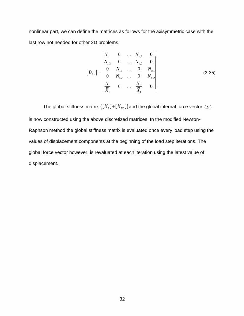
nonlinear part, we can define the matrices as follows for the axisymmetric case with the
last row not needed for other 2D problems.
1,1 ,1
1,2 ,2
1,1 ,1
1,2 ,2
1
1 1
0 ... 0
0 ... 0
0 ... 0
0 ... 0
0 ... 0
NL
n
n
n
n
n
N N
N
B
N
N N
N N
NN
X X
(3-35)
The global stiffness matrix [ ] [ ]L NLK K and the global internal force vector { }F
is now constructed using the above discretized matrices. In the modified Newton-
Raphson method the global stiffness matrix is evaluated once every load step using the
values of displacement components at the beginning of the load step iterations. The
global force vector however, is revaluated at each iteration using the latest value of
displacement.

33
CHAPTER 4 IMPLICIT BOUNDARY METHOD FOR NONLINEAR ANALYSIS
In this chapter we extend the theory of Implicit of Boundary method to non-linear
analysis. The major advantage of IBFEM is the use of structured background mesh
instead of a conforming mesh. This potentially can eliminate the difficulty of mesh
generation that is required for any FEA analysis.
Application of IBFEM to static problems such as elastic problems and heat
conduction problems have been demonstrated in past work, in this chapter we extend it
to nonlinear analysis.
Governing Equation for Nonlinear Analysis Using IBFEM
To impose essential boundary conditions, in the implicit boundary method, the
displacement and virtual displacement are expressed as:
g a s a
i i i i i iu Du u u u (4-1)
g
i i iu D u (4-2)
Here iD is equal to unity inside the solid as well as on the boundaries that do not
have any Dirichlet boundary conditions specified. Within elements that contain a
boundary with a Dirichlet boundary condition specified on the i th component of
displacement, iD is constructed as an approximate step function whose value goes to
zero at the boundary as:
0 0
( ) (2 ) 0 1,2,3
1
D i
(4-3)

34
Here is the distance function from the boundary of interest. Therefore at that
boundary since 0iD , the specified boundary condition a
i iu u is guaranteed to be
enforced. Here a
iu is the boundary value function that must be constructed such that it
has the specified boundary condition values at the boundary. g
iu is constructed by
piece-wise interpolation or approximation using the shape functions of the element.
The use of Dirichlet function changes the structure of the displacements
assumed within each element that result in a modified shape function within the region
where the step function transitions from one to zero. In this transition region near the
boundary, we have,
g a g a
i i k ik i ik ik i
k k
u D N u u N u u (4-4)
, ,
g aii j ik j ik i
kj
uu N u u
X
(4-5)
,
ik k iik j i k
j j j
N N DN D N
X X X
(4-6)
Where, ik i kN D N is the modified shape function for the kth node. Note within the
elements that do not have a boundary with displacement specified, 1iD , therefore
ik kN N and , ,ik j k jN N which implies that all these elements are identical to the
traditional finite elements except that some of the elements on the boundary may be
partially inside and partially outside the domain of analysis. In these cases, the stiffness
is computed accurately by only integrating over the region of the element that is within
the domain. To do so, the element could be subdivided into triangles or tetrahedron so

35
that the integration may be carried over only those triangles or tetrahedrons that are
within the domain.
Discretization Using IBFEM
In the traditional nonlinear finite element procedure [17-18], the preceding
equation is discretized by deriving matrix equations that relate the quantities of interest
with the nodal values of displacement or change in displacement. As is already
described in Chapter 3 this equation(4-8) yields a global system of equations of the
form:
[ ] [ ] { } { } { }L NLK K X R F (4-7)
To get the global tangent stiffness matrix ([ ] [ ])L NLK K and the internal force
vector { }F we define linear and nonlinear strain displacement matrices. Using the
earlier definition of the strain-displacement matrices equations (3-25)(3-26)(3-27) and
the solution structure equations (4-1, 4-2) we get the following matrices,
0 1L L LB B B (4-8)
11,1 1 ,1
21,2 2 ,2
0 11,2 21,1 1 ,2 2 ,1
111
1 1
0 ... 0
0 ... 0
...
0 ... 0
n
n
L n n
n
N N
N N
B N N N N
NN
X X
(4-9)
11 1 ,1 21 2 ,1
12 1 ,2 22 2 ,2
1 11 1 ,2 12 1 ,1 21 2 ,2 22 2 ,1
133
1
( ) ( )
0
n n
n n
L n n n n
n
l N l N
l N l N
B l N l N l N l N
Nl
X
(4-10)

36
Where, ,
ik k iik j i k
j j j
N N DN D N
X X X
, 1 1
1
nk
ik
k
X N X
, 11 ,1 1
1
( )n
ik k
k
l N u t
,
22 ,2 2
1
( )n
ik k
k
l N u t
, 21 ,1 2
1
( )n
ik k
k
l N u t
, 12 ,2 1
1
( )n
ik k
k
l N u t
, 1
133
( )n
ik k
k
N u t
lX
and
n is the number of nodes per element.
11,1 1 ,1
11,2 1 ,2
21,1 2 ,1
21,2 2 ,2
111
1 1
0 ... 0
0 ... 0
0 ... 0
0 ... 0
0 ... 0
N
n
n
n
n
L
n
N N
N N
N N
N N
NN
B
X X
(4-11)
In all the above relations we use the modified shape function.
Constructing The Global Stiffness Matrix
The construction of the global stiffness can therefore be implemented by using
first the unmodified shape function kN in equations (3-25)-(27) for all the elements to
construct element stiffness matrices and assembling them. Thereafter, the stiffness
associated with the transition region where the step function transitions from one to zero
can be computed as a line integral (for 2D and shell) or surface integrals (for 3D) as:
0
0
[ ] [ ] [ ][ ]
a
a T
L L LK B C B d d
(4-12)
0
0
[ ] [ ] [ ][ ]
a
a T
NL NL NLK B S B d d
(4-13)
These can be thought of as the stiffness of the boundary a and are also
assembled in the global stiffness matrix. Note that the integration is first performed

37
normal to the boundary with respect to the distance function and thereafter a line or
surface integration is performed over the boundary a .

38
CHAPTER 5 RESULT AND DISCUSSION
A few numerical examples are employed to verify the accuracy of non-linear
analysis using background mesh and Implicit Boundary Finite Element Method (or
IBFEM).
In the following examples we study the deformation of a cantilever subjected to
end shear force [19] modeled using 3D shell elements. We also look at a plane stress
and an axis-symmetric example modeled using 2D elements and compare the results
with commercial software.
2D Examples
In this section, we will present examples using 2D elements.
Plane Stress: A Plate Subjected to Uniform Pressure at the Top
In this example a plate with a large width subjected to uniform pressure at the top
is modelled as a plane stress example. Figure 5-1 shows the cross section with
dimensions 100L , 5h . A uniform pressure is applied along the top surface of the
structure and it is clamped at one end. The model with boundary conditions is shown in
Figure 5-2. The material properties were Young’s modulus 61.2 10E , Poisson's ratio
0.1 . An initial pressure of 10P is applied.
The mesh used for the analysis using IBFEM is shown in figure 5-2 and it
consists of 16 Node B-Spline elements. The mesh density for this model is 40 4 1 . A
model for the same structure was also created in ABAQUS which uses 164 quadratic
quadrilateral elements of type CPS8R. For validation, the maximum displacement,
computed in the structure using IBFEM and Abaqus, is compared.

39
In this example we also look at the stress plots for Von-Mises and stress in radial
direction. The stress contours obtained from IBFEM show good correlation with stress
contours obtained from Abaqus.
Figure 5-1. A plane strain plate subjected to uniform pressure at the top
Figure 5-2. FE Model
Figure 5-3. Displacement at P=100 A). IBFEM B). Abaqus
A B

40
Figure 5-4. Stress along x-direction A). IBFEM B). Abaqus
Figure 5-5. Von-Mises Stress A). IBFEM B). Abaqus
B A
A B

41
Figure 5-6. Maximum Deflection vs Pressure 𝑃 A). IBFEM vs Abaqus B). Convergence of different mesh densities.
Table 5-1. Maximum deflection comparison.
P Max. deflection P Max. deflection IBFEM Abaqus IBFEM Abaqus
0 0 0 60 56.25 55.41 10 10.48 10.02 70 62.94 62.58 20 20.78 20.01 80 68.74 68.89 30 30.71 29.59 90 73.58 74.3 40 40.04 38.8 100 77.6 78.79 50 48.59 47.45
Plane Stress: Thin Frame-like Structure
In this example a thin frame-like structure is modelled using 2D plane stress
elements. The structure is as shown in figure 5-7. This structure is rigidly clamped at
both the ends and a uniform pressure is applied at the top. The model with boundary
conditions is shown in figure 5-8(A). The material properties were Young’s modulus
61.2 10E , Poisson's ratio 0 . The structure has a cross-section of5 0.1 . An initial
pressure of 100P is applied.
The mesh used for the analysis using IBFEM is shown in figure 5-8(A) and it
consists of 9 Node biquadratic elements. The mesh density for this model is 60 60 1 . A
A B

42
model for the same structure was also created in ABAQUS which uses 164 quadratic
quadrilateral elements of type CPS8R. For validation, the maximum displacement,
computed in the structure using IBFEM and Abaqus, is compared.
As seen in the figure, the nonlinearity is mild for this problem but at large
deformation the results from IBFEM and Abaqus are close and deviate significantly from
the linear solution. Table 5-2 lists the maximum deflection of the structure and the
corresponding applied pressure for the results obtained using IBFEM and Abaqus.
Figure 5-7. Thin beam structure
Figure 5-8. Thin beam structure A). FE model B). Structure Displacement
A B

43
Figure 5-9. Maximum Deflection vs Pressure 𝑃 A). IBFEM vs Abaqus B). Convergence study
Table 5-2. Maximum deflection comparison.
P Max. deflection P Max. deflection IBFEM Abaqus IBFEM Abaqus
100 3.640 3.702 260 10.111 9.973 120 4.403 4.472 280 10.971 10.760 140 5.178 5.249 300 11.850 11.650 160 5.969 6.031 320 12.740 12.340 180 6.773 6.816 340 13.660 13.130 200 7.583 7.603 360 14.851 13.920 220 8.410 8.393 380 15.510 15.310 240 9.248 9.182 400 16.480 15.500
Axisymmetric: Thin Disk
In this example a thin disk like structure is modelled using 2D Axisymmetric
elements. Figure 5-10 shows the cross section with dimensions and the revolved
geometry of the structure. A uniform pressure is applied along the top surface of the
disk and the disk is clamped along its edges. The model with boundary conditions is
shown in Figure 5-11. The material properties were Young’s modulus 61.2 10E ,
Poisson's ratio 0.1 . An initial pressure of 10P is applied.
A B

44
The mesh used for the analysis using IBFEM is shown in Figure 5-11 and it
consists of 4 Node quadratic elements. The mesh density for the model is 40 10 1 . A
model for the same structure was also created in SolidWorks. For validation, the
maximum displacement, computed in the structure using IBFEM and SolidWorks, is
compared. The results are also listed in Table 5-3.
In this example we also look at the stress plots for Von-Mises and stress in radial
direction. The stress contours obtained from IBFEM show good correlation with stress
contours obtained from Abaqus.
Figure 5-10. Thin Disk A). Section B). Revolved geometry
Figure 5-11. FE Model
A B

45
Figure 5-12. Displacement at P=100
Figure 5-13. Von-Mises Stress A). IBFEM B). Abaqus
Figure 5-14. Maximum Deflection vs Pressure 𝑃 A). IBFEM vs SolidWorks B).
Convergence study
A B

46
Table 5-3. Maximum deflection comparison.
P Max. deflection P Max. deflection
IBFEM SW IBFEM SW
10 2.240 2.402 60 11.221 11.160 20 4.575 4.787 70 12.570 12.280 30 6.745 6.801 80 13.810 13.310 40 8.671 8.475 90 14.950 14.250 50 9.728 9.904 100 16.021 15.130
3D Shell Example
In this section, we will present examples using 3D elements.
Cantilever Subjected to End Shear Force
In this example, we consider a thin cantilevered plate which is subjected to end
shear force and is a benchmark problem that has been used in many studies [20]. The
thin plate is illustrated in Figure 5-15 and its dimension are 10L , 1b and 0.1h . The
Young’s modulus of the material is 61.2 10E and the Poisson's ratio 0 . We use 3D
shell element to model the plate and the displacement at the tip is used for the
comparison and validation.
The background mesh used for this analysis is shown in the Figure 5-16(A)
which consists of 3D cubic B-spline elements. The geometry is a surface which passes
through these elements. The stiffness matrix of these elements is computed by
integrating over the part of the surface that passes through the elements as well as
through the thickness of the shell normal to the surface [3]. The shear load is applied by
first computing the work equivalent nodal load for the nodes of the element that contains
the edge on which the load is acting and then assembling this element load vector to
the global external load vector.

47
The tip deflection is shown in Figure 5-16(B) with no scaling to show the
magnitude of the deflection. The deflection is compared with the applied load in Figure
5-17 and listed in Table 5-4. Again the results from IBFEM and the exact solution
reported in [ref] match very closely.
Figure 5-15. Cantilever beam subjected to end shear load
Figure 5-16. Cantilever beam model A). Mesh Model. B) Cantilever plate deflection at P-
2.4N.
Figure 5-17. Deflection vs Load graph.
B A

48
Table 5-4. Vertical tip deflections for the cantilever loaded with end shear force.
P Wtip P Wtip IBFEM Exact IBFEM Exact
0.2 0.651 0.663 1.4 3.982 3.912 0.4 1.291 1.309 1.6 4.350 4.292 0.6 1.957 1.992 1.8 4.710 4.631 0.8 2.570 2.493 2.0 5.042 4.933 1.0 3.071 3.015 2.2 5.389 5.202 1.2 3.496 3.488 2.4 5.701 5.444
Application in Flexural Hinge Design
Flexural hinges and flexure based mechanism are used for many macro- and
microscale applications. Flexure mechanisms are designed to provide guided motion
through elastic deformation. They can be used in place of sliding or rolling joints. They
are generally used in applications that demand high precision, design simplicity, minimal
assembly or long operating life [21, 22].
In our example we use a single-axis flexure hinge as shown in figure 5-18 [23].
This flexural design has a circular cut-out on either side of the blank which forms a
necked-down section. These kinds of flexures are popular for its simplistic design, ease
of manufacturing and high off-axis stiffness.
Figure 5-18. Dimensions, Forces and coordinates of a flexural hinge

49
The flexure used for this example can be defined with these physical and
geometric parameters: 10 29.326 10 /E N m , 10 23.296 10 /G N m , 7.68b mm ,
0.892t mm , 3.465R mm , 36.2o
m . A pressure of 100MPa is applied on the face that
has the y coordinate as its normal. We model the hinge as a plane stress problem.
The mesh used for the analysis using IBFEM is shown in Figure 5-19 and it
consists of 9 Node BSpline elements. The mesh density for the model is 9 31 1 with
element size 0.25. A model for the same structure was also created in SolidWorks. For
validation, the maximum displacement and Von-mises stress contour at the neck,
computed in the structure using IBFEM and SolidWorks, is compared.
Figure 5-19. FE Model
Figure 5-20. Maximum Displacement comparison A). IBFEM B). SW
A B

50
Figure 5-21. Von-mises stress contours A). IBFEM B). SW
A B

51
CHAPTER 6 CONCLUSION
Summary
The extension of implicit boundary method for geometrically nonlinear problems
was described in this thesis and used to perform mesh independent analysis using a
background mesh. Initially, IBFEM and its solution structure was explained. The
governing equations for traditional finite element method were derived and explained.
These equations were derived using Total lagrangian approach. Based on the IBFEM
solution structure we derive the governing equations for boundary elements with
essential boundary condition. The governing equation (4-8) derived using the Dirichlet
function or the essential boundary function only affect the elements at the boundary with
essential boundary condition imposed. For the rest of the elements the stiffness matrix
computation and the residual load vector are calculated same as traditional FEM.
The main challenge in the process is in accurately computing the stiffness
associated with the fixed boundaries in the equation (4-14)-(15). It was found that this
stiffness is more accurately computed when it is assumed that within the transition
region near the boundary the nonlinear part of the stiffness and the internal force are
negligible. This is a reasonable assumption near fixed boundaries since the
displacement near such boundaries will be small. There is a definite advantage in using
the TL formulation for large deformation as opposed to the UL formulation when using a
background mesh for analysis. The elements in the background mesh are undistorted
regular shaped rectangles and cuboids which allow very accurate integration. In the TL
formulation since the equations are written with respect to the original configuration the
mesh in the original configuration remains undistorted and retains the advantage of
52
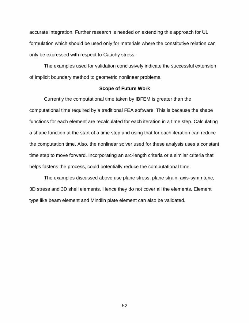
accurate integration. Further research is needed on extending this approach for UL
formulation which should be used only for materials where the constitutive relation can
only be expressed with respect to Cauchy stress.
The examples used for validation conclusively indicate the successful extension
of implicit boundary method to geometric nonlinear problems.
Scope of Future Work
Currently the computational time taken by IBFEM is greater than the
computational time required by a traditional FEA software. This is because the shape
functions for each element are recalculated for each iteration in a time step. Calculating
a shape function at the start of a time step and using that for each iteration can reduce
the computation time. Also, the nonlinear solver used for these analysis uses a constant
time step to move forward. Incorporating an arc-length criteria or a similar criteria that
helps fastens the process, could potentially reduce the computational time.
The examples discussed above use plane stress, plane strain, axis-symmteric,
3D stress and 3D shell elements. Hence they do not cover all the elements. Element
type like beam element and Mindlin plate element can also be validated.

53
LIST OF REFERENCES
1. A.V. Kumar, R. Burla, S. Padmanabhan, L.X. Gu, “Finite element analysis using nonconforming mesh”, Journal of Computing and Information Science in Engineering, Transactions of ASME, Vol. 8., No. 3, 031005 (11 pages) doi:10.1115/1.2956990.
2. Burla R. and Kumar, A. V., 2008, “Implicit boundary method for analysis using uniform B-spline basis and structured grid”, International Journal for Numerical Methods in Engineering, Vol 76, No. 13 pp. 1993-2028.
3. A.V. Kumar, P.S. Periyasamy, “Mesh independent analysis of shell-like structures”, International Journal for Numerical Methods in Engineering
4. A.V. Kumar, R. Burla, S. Padmanabhan, “Implicit boundary method for finite element analysis using non-conforming mesh or grid”, International Journal for Numerical Methods in Engineering, Vol. 74., 1421-1447
5. Zhang Z. and Kumar A. V., Modal Analysis using implicit boundary finite element method, Proceedings of the ASME 2014 International Design Engineering Technical Conferences & Computers and Information in Engineering Conference, DETC2014-35100, 2014
6. G.R. Liu, Mesh free methods: moving beyond the finite element method, CRC Press, Boca Raton, 2003
7. Y.T. Gu,. Meshfree methods and their comparisons, Int. J. Comput. Methods 2 (2005) 477–515.
8. P. Lancaster, K. Salkauskas, Surfaces generated by moving least squares methods, Math. Comput. 37 (1981) 141–158.
9. Y.Y. Lu, T. Belytschko, L. Gu, A new implementation of the element free Galerkin method, Comput. Methods Appl. Mech. Engrg. 113 (1994) 397–414.
10. Z. D. Han, S. N. Atluri, The meshless local Petrov-Galerkin (MLPG) approach for 3-dimensional elasto-dynamics, CMC-Comput. Mater. Con. 1 (2004) 129–140.
11. G.R. Liu, X.L. Chen, A mesh-free method for static and free vibration analyses of thin plates of complicated shape, J. of Sound Vibrat. 241 (2001) 839-855.
12. Y.T. Gu, G.R. Liu, A meshless local Petrov-Galerkin (MLPG) method for free and forced vibration analyses for solids, Comput. Mech. 27 (2001) 188-198.
13. T. Belytschko, C. Parimi, N. Moes, N. Sukumar, S. Usui, Structured extended finite element methods for solids defined by implicit surfaces, Int. J. Numer. Methods Engrg. 56 (2003) 609–635.

54
14. Rvachev, V.L., and Shieko, T.I., 1995, “R-functions in Boundary value problems in Mechanics,” Appl. Mech. Rev., 48, pp. 151-188
15. Shapiro V, Tsukanov I. Meshfree simulation of deforming domains. Computer-Aided Design 1999; 31:459–471.
16. H¨ollig K, Reif U, Wipper J. Weighted extended B-spline approximation of Dirichlet problems. SIAM Journal on Numerical Analysis 2002; 39:442–462.
17. Klaus Jurgen Bathe and Arthur P. Cimento, Some practical procedures for the solution of nonlinear finite element equations, Computer methods in applied mechanics and engineering. 22 (1980) 59-85.
18. Kim Nam Ho, Introduction to Nonlinear Finite Element Analysis. Springer(2015)
19. K.Y. Sze, X.H. Liu, S.H. Lo, Popular benchmark problems for geometric nonlinear analysis of shells, Finite Elements in Analysis and Design 40 (2004) 1551-1569
20. H. Parisch, Large displacements of shells including material nonlinearities, Computer methods in applied mechanics and engineering 27 (1981) 183-214.
21. Howell, L. L., 2001, Compliant Mechanisms, Wiley, New York.
22. Smith, S. T., 2000, Flexures: Elements of Elastic Mechanisms, Gordon & Breach, Amsterdam, Netherlands
23. Yingfei Wu and Zhaoying Zhou, 2002, Design calculations for flexure hinges, Review of Scientific Instruments
24. Rvachev VL, Sheiko TI, Shapiro V, Tsukanov I. Transfinite interpolation over implicitly defined sets. ComputerAided Geometric Design 2001; 18:195–220.

55
BIOGRAPHICAL SKETCH
Nikhil Bhosale was born in Pune, Maharashtra (India). He received his Bachelor
of Technology in mechanical engineering from Visvesvaraya National Institute of
Technology, Nagpur in 2012. After his graduation, he worked as a Senior Engineer at
Bajaj Auto Ltd. in the Computer Aided Engineering department. He received the
Employee achievement award in 2014 for his excellent initiatives during his work at
Bajaj Auto Ltd. In 2014 he enrolled in the Master of Science program in mechanical
engineering at University of Florida. He received his master’s degree in mechanical
engineering in May 2016 from University of Florida. His areas of specialization include
nonlinear finite element analysis, background mesh finite element methods, numerical
methods, optimization design and software development using Object Orientation
Programming Techniques.