() ρ = ρ − − ρ − −Δ − − Δ · spring 2006 process dynamics, operations, and control...
TRANSCRIPT
Spring 2006 Process Dynamics, Operations, and Control 10.450 Lesson 6: Exothermic Tank Reactor 6.0 context and direction A tank reactor with an exothermic reaction requires a more elaborate system model, because its outputs are temperature and composition. Furthermore, the model is nonlinear, which forces us to make a linear approximation to solve it. We will add the derivative mode to our PI controller to increase both stability and responsiveness. The closed loop will show how automatic control can stabilize an inherently unstable process.
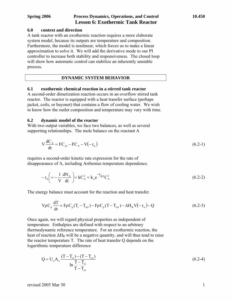
DYNAMIC SYSTEM BEHAVIOR 6.1 exothermic chemical reaction in a stirred tank reactor A second-order dimerization reaction occurs in an overflow stirred tank reactor. The reactor is equipped with a heat transfer surface (perhaps jacket, coils, or bayonet) that contains a flow of cooling water. We wish to know how the outlet composition and temperature may vary with time. 6.2 dynamic model of the reactor With two output variables, we face two balances, as well as several supporting relationships. The mole balance on the reactant A
( AAAiA rVFCFC
dtdCV −−−= ) (6.2-1)
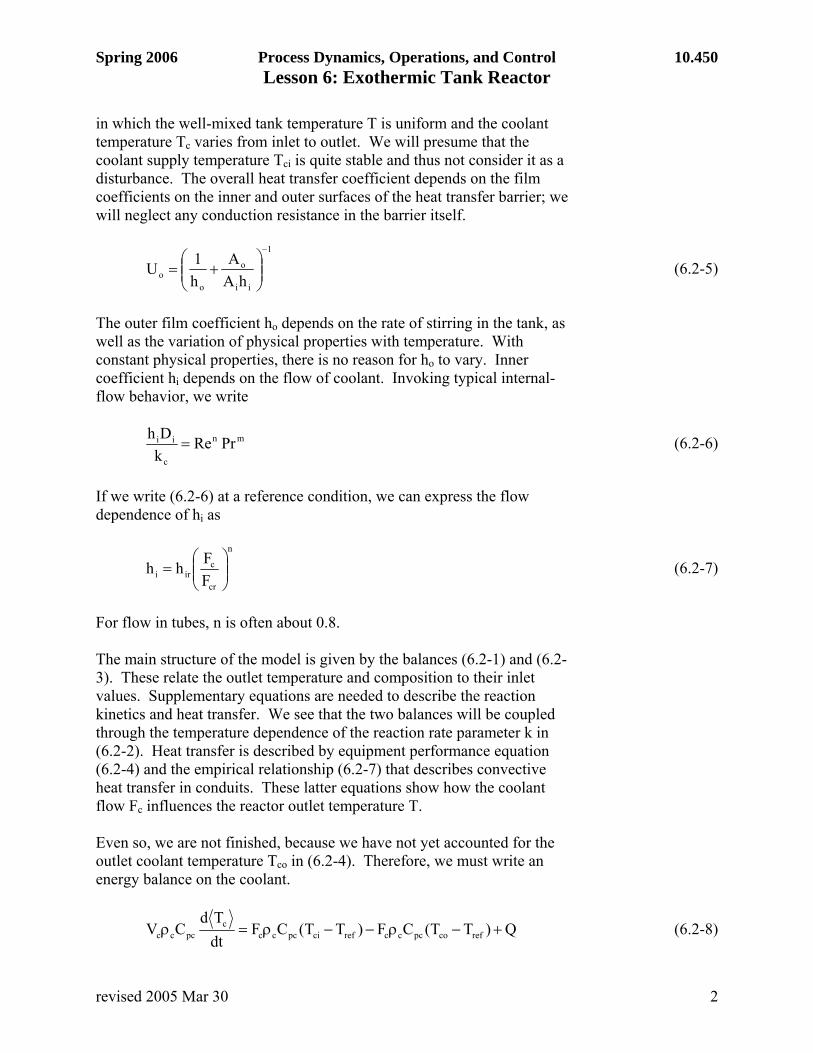
requires a second-order kinetic rate expression for the rate of disappearance of A, including Arrhenius temperature dependence.
2A
RTE
o2A
AA CekkC
dtdN
V1r
−==⎟
⎠⎞
⎜⎝⎛ −=− (6.2-2)
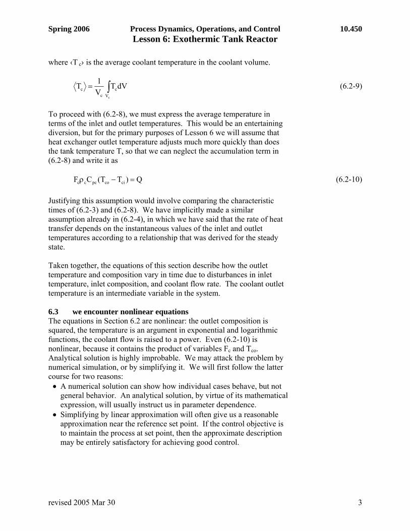
The energy balance must account for the reaction and heat transfer.
( ) QrVH)TT(CF)TT(CFdtdTCV ARrefprefipp −−Δ−−ρ−−ρ=ρ (6.2-3)
Once again, we will regard physical properties as independent of temperature. Enthalpies are defined with respect to an arbitrary thermodynamic reference temperature. For an exothermic reaction, the heat of reaction ΔHR will be a negative quantity, and will thus tend to raise the reactor temperature T. The rate of heat transfer Q depends on the logarithmic temperature difference
co
ci
cocioo
TTTTln
)TT()TT(AUQ
−−
−−−= (6.2-4)
revised 2005 Mar 30 1
Spring 2006 Process Dynamics, Operations, and Control 10.450 Lesson 6: Exothermic Tank Reactor in which the well-mixed tank temperature T is uniform and the coolant temperature Tc varies from inlet to outlet. We will presume that the coolant supply temperature Tci is quite stable and thus not consider it as a disturbance. The overall heat transfer coefficient depends on the film coefficients on the inner and outer surfaces of the heat transfer barrier; we will neglect any conduction resistance in the barrier itself.
1
ii
o
oo hA
Ah1U
−
⎟⎟⎠
⎞⎜⎜⎝
⎛+= (6.2-5)
The outer film coefficient ho depends on the rate of stirring in the tank, as well as the variation of physical properties with temperature. With constant physical properties, there is no reason for ho to vary. Inner coefficient hi depends on the flow of coolant. Invoking typical internal-flow behavior, we write
mn
c
ii PrRekDh
= (6.2-6)
If we write (6.2-6) at a reference condition, we can express the flow dependence of hi as
n
cr
ciri F
Fhh ⎟⎟⎠
⎞⎜⎜⎝
⎛= (6.2-7)
For flow in tubes, n is often about 0.8. The main structure of the model is given by the balances (6.2-1) and (6.2-3). These relate the outlet temperature and composition to their inlet values. Supplementary equations are needed to describe the reaction kinetics and heat transfer. We see that the two balances will be coupled through the temperature dependence of the reaction rate parameter k in (6.2-2). Heat transfer is described by equipment performance equation (6.2-4) and the empirical relationship (6.2-7) that describes convective heat transfer in conduits. These latter equations show how the coolant flow Fc influences the reactor outlet temperature T. Even so, we are not finished, because we have not yet accounted for the outlet coolant temperature Tco in (6.2-4). Therefore, we must write an energy balance on the coolant.
Q)TT(CF)TT(CFdtTd
CV refcopcccrefcipcccc
pccc +−ρ−−ρ=ρ (6.2-8)
revised 2005 Mar 30 2
Spring 2006 Process Dynamics, Operations, and Control 10.450 Lesson 6: Exothermic Tank Reactor where ‹T c› is the average coolant temperature in the coolant volume.
∫=cV
cc
c dVTV1T (6.2-9)
To proceed with (6.2-8), we must express the average temperature in terms of the inlet and outlet temperatures. This would be an entertaining diversion, but for the primary purposes of Lesson 6 we will assume that heat exchanger outlet temperature adjusts much more quickly than does the tank temperature T, so that we can neglect the accumulation term in (6.2-8) and write it as
Q)TT(CF cicopccc =−ρ (6.2-10) Justifying this assumption would involve comparing the characteristic times of (6.2-3) and (6.2-8). We have implicitly made a similar assumption already in (6.2-4), in which we have said that the rate of heat transfer depends on the instantaneous values of the inlet and outlet temperatures according to a relationship that was derived for the steady state. Taken together, the equations of this section describe how the outlet temperature and composition vary in time due to disturbances in inlet temperature, inlet composition, and coolant flow rate. The coolant outlet temperature is an intermediate variable in the system. 6.3 we encounter nonlinear equations The equations in Section 6.2 are nonlinear: the outlet composition is squared, the temperature is an argument in exponential and logarithmic functions, the coolant flow is raised to a power. Even (6.2-10) is nonlinear, because it contains the product of variables Fc and Tco. Analytical solution is highly improbable. We may attack the problem by numerical simulation, or by simplifying it. We will first follow the latter course for two reasons: • A numerical solution can show how individual cases behave, but not
general behavior. An analytical solution, by virtue of its mathematical expression, will usually instruct us in parameter dependence.
• Simplifying by linear approximation will often give us a reasonable approximation near the reference set point. If the control objective is to maintain the process at set point, then the approximate description may be entirely satisfactory for achieving good control.
revised 2005 Mar 30 3
Spring 2006 Process Dynamics, Operations, and Control 10.450 Lesson 6: Exothermic Tank Reactor 6.4 making linear approximations with Taylor series Given a function f, we specify some reference value of the independent variables, and represent the function in the neighborhood of that reference point as a series of terms. For a function of one variable:
( 2rr
xr )xx(O)xx(
dxdf)x(f)x(f
r
−+−+= ) (6.4-1)
For a function of more than one variable:
( ),...)yy(,)xx(O...)yy(yf
)xx(xf,...)y,x(f,...)y,x(f
2r
2rr
,...y,x
r,...y,x
rr
rr
rr
−−++−∂∂+
−∂∂+=
(6.4-2)
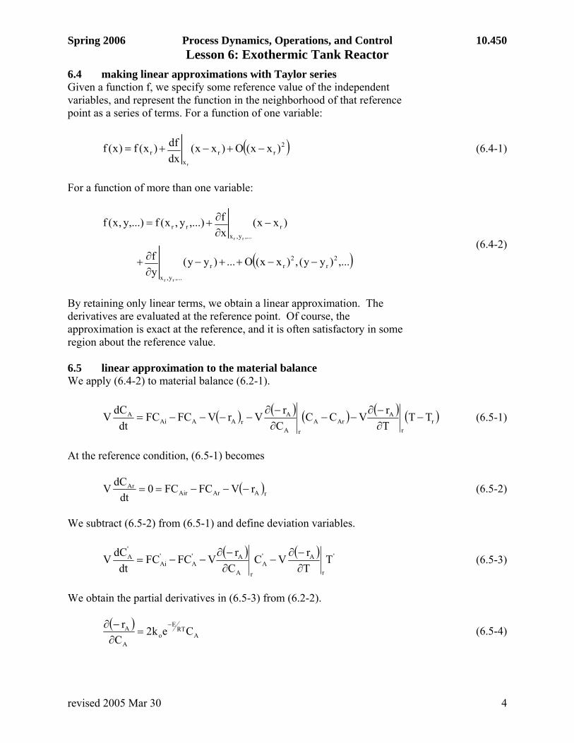
By retaining only linear terms, we obtain a linear approximation. The derivatives are evaluated at the reference point. Of course, the approximation is exact at the reference, and it is often satisfactory in some region about the reference value. 6.5 linear approximation to the material balance We apply (6.4-2) to material balance (6.2-1).
( ) ( ) ( ) ( ) ( rr
AArA
rA
ArAAAi
A TTTrVCC
CrVrVFCFC
dtdCV −
∂−∂
−−∂−∂
−−−−= ) (6.5-1)
At the reference condition, (6.5-1) becomes
( rAArAirAr rVFCFC0
d)
tdCV −−−== (6.5-2)
We subtract (6.5-2) from (6.5-1) and define deviation variables.
( ) ( ) '
r
A'A
rA
A'A
'Ai
'A T
TrVC
CrVFCFC
dtdCV
∂−∂
−∂−∂
−−= (6.5-3)
We obtain the partial derivatives in (6.5-3) from (6.2-2).
( )A
RTE
oA
A Cek2C
r −=
∂−∂ (6.5-4)
revised 2005 Mar 30 4
Spring 2006 Process Dynamics, Operations, and Control 10.450 Lesson 6: Exothermic Tank Reactor
( )ArrAr
RTE
orA
A Ck2Cek2C
rr ==
∂−∂ −
(6.5-5)
( ) 2
ART
E
2oA Ce
RTEk
Tr −
=∂−∂ (6.5-6)
( ) 2Ar2
rr
2Ar
RTE
2r
or
A CRT
EkCeRT
EkTr
r ==∂−∂ −
(6.5-7)
Here kr is the rate constant at the reference condition.
rRTE
or ekk−
= (6.5-8) We substitute (6.5-5) and (6.5-7) into linearized material balance (6.5-3).
'2Ar2
rr
'AArr
'A
'Ai
'A TC
RTEVkCCVk2FCFC
dtdCV −−−= (6.5-9)
This is a first-order lag equation, which is more apparent if it is placed into standard form
0)0(CTKCCdt
dC 'A
'CT
'Ai
R
C'A
'A
C =+ττ
=+τ (6.5-10)
where
2Arr2
rCCT
ArrR
RC
R
CkRT
EK
Ck21
FV
τ−=
τ+τ
=τ
=τ
(6.5-11)
τR is the residence time of the tank, important to reactor conversion. The time constant τC (smaller than τR) characterizes the dynamics of composition change. The group KCT is the gain for the effect of temperature on composition in the reactor. The negative sign shows that an increase in operating temperature will reduce the exit concentration of reactant A (by way of increasing the reaction rate constant).
revised 2005 Mar 30 5
Spring 2006 Process Dynamics, Operations, and Control 10.450 Lesson 6: Exothermic Tank Reactor The steady state mole balance in (6.5-2) has significance beyond serving as a reference condition for deviation variables. It also constrains the relationship between the tank composition and temperature (within the rate constant kr) at steady state. 6.6 similarly approximating the energy balance We apply (6.4-2) to energy balance (6.2-3).
( ) ( ) ( ) ( ) ( )
( ) ( )crcrc
rr
r
rr
ARArA
rA
ARrAR
pipp
FFFQTT
TQQ
TTTrVHCC
CrVHrVH
TCFTCFdtdTCV
−∂∂
−−∂∂
−−
−∂−∂
Δ−−∂−∂
Δ−−Δ−
ρ−ρ=ρ
(6.6-1)
At the reference condition, (6.6-1) becomes
( ) rrARrpirpr
p QrVHTCFTCF0dt
dTCV −−Δ−ρ−ρ==ρ (6.6-2)
We subtract (6.6-2) from (6.6-1) and define deviation variables.
( ) ( )
'c
rc
'
r
'
r
AR
'A
rA
AR
'p
'ip
'
p
FFQT
TQ
TTrVHC
CrVHTCFTCF
dtdTCV
∂∂
−∂∂
−
∂−∂
Δ−∂−∂
Δ−ρ−ρ=ρ
(6.6-3)
The reaction rate partial derivatives are given in (6.5-5) and (6.5-7). To obtain the heat transfer rate partial derivatives, we combine the heat transfer expressions (6.2-4) through (6.2-7) with the coolant energy balance (6.2-10) to eliminate intermediate variable Tco.
( )⎥⎥⎦
⎤
⎢⎢⎣
⎡
⎪⎭
⎪⎬⎫
⎪⎩
⎪⎨⎧
⎟⎟⎠
⎞⎜⎜⎝
⎛+
ρ−
−−ρ=−1
nciri
ncro
opccc
ocipccc FhA
FAh1
CFAexp1TTCFQ (6.6-4)
The partial derivatives are
⎥⎥⎦
⎤
⎢⎢⎣
⎡
⎪⎭
⎪⎬⎫
⎪⎩
⎪⎨⎧
⎟⎟⎠
⎞⎜⎜⎝
⎛+
ρ−
−ρ=∂∂
−1
nciri
ncro
opccc
opccc FhA
FAh1
CFAexp1CF
TQ (6.6-5)
revised 2005 Mar 30 6
Spring 2006 Process Dynamics, Operations, and Control 10.450 Lesson 6: Exothermic Tank Reactor
[ rpcccrr
1CFTQ
β−ρ=∂∂ ] (6.6-6)
( )
( )⎥⎥⎦
⎤
⎢⎢⎣
⎡⎟⎟⎠
⎞⎜⎜⎝
⎛+−
⎪⎭
⎪⎬⎫
⎪⎩
⎪⎨⎧
⎟⎟⎠
⎞⎜⎜⎝
⎛+
ρ−
⎟⎟⎠
⎞⎜⎜⎝
⎛+
−−
⎥⎥⎦
⎤
⎢⎢⎣
⎡
⎪⎭
⎪⎬⎫
⎪⎩
⎪⎨⎧
⎟⎟⎠
⎞⎜⎜⎝
⎛+
ρ−
−−ρ=∂∂
−−−
−
nciri
ncro
1
nciri
ncro
o
1
nciri
ncro
opccc
o
1
nciri
ncro
oc
cio
1
nciri
ncro
opccc
ocipcc
c
FhAnFA
FhAFA
h11
FhAFA
h1
CFAexp
FhAFA
h1
FTTA
FhAFA
h1
CFAexp1TTC
FQ
(6.6-7)
( )[ ] ( )⎥⎦
⎤⎢⎣
⎡−
−β−β−−ρ=
∂∂
iri
oor
cr
ciroorrrcirpcc
rc hAnAU1
FTTAU1TTC
FQ (6.6-8)
in which
1
iri
o
oor hA
Ah1U
−
⎟⎟⎠
⎞⎜⎜⎝
⎛+= (6.6-9)
and
⎪⎭
⎪⎬⎫
⎪⎩
⎪⎨⎧
ρ−
=βpcccr
oorr CF
AUexp (6.6-8)
The argument of the exponential function in (6.6-8) is the “number of transfer units”, used in models of heat exchangers (Incropera and DeWitt, Sec. 11.4). We substitute (6.5-5), (6.5-7), (6.6-6), and (6.6-8) into linearized energy balance (6.6-3) to obtain another first order lag equation.
0)0(TFKCKTTdt
dT ''cht
'ATC
'i
R
T''
T =++ττ
=+τ (6.6-10)
where
revised 2005 Mar 30 7
Spring 2006 Process Dynamics, Operations, and Control 10.450 Lesson 6: Exothermic Tank Reactor
( )
( ) ( )⎥⎥⎦
⎤
⎢⎢⎣
⎡β−−⎟⎟
⎠
⎞⎜⎜⎝
⎛−
ρβ
ρ
−ρ
ττ
=
ρΔ
τ−=
ρΔ
τ+β−ρρ
+
τ=τ
riri
oor
pcccr
oorr
p
cirpcc
R
Tht
Arrp
rTTC
2Arr2
rp
rRr
p
pcccr
RT
1hAAnU1
CFAU
CFTTC
K
CkCH2K
CkRT
ECH1
CFCF
1
(6.6-11)
Once again, standard-form parameters have been defined. The thermal time constant τT characterizes the dynamics of temperature change, and KTC and Kht are gains for composition and heat transfer disturbances. 6.7 deriving transfer functions by Laplace transform and block diagram Laplace transforms may be performed on the mole balance (6.5-10) and the energy balance (6.6-10).
)s(TK)s(C)s(C)1s( 'CT
'Ai
R
C'AC +
ττ
=+τ (6.7-1)
)s(FK)s(CK)s(T)s(T)1s( 'cht
'ATC
'i
R
T'T ++
ττ
=+τ (6.7-2)
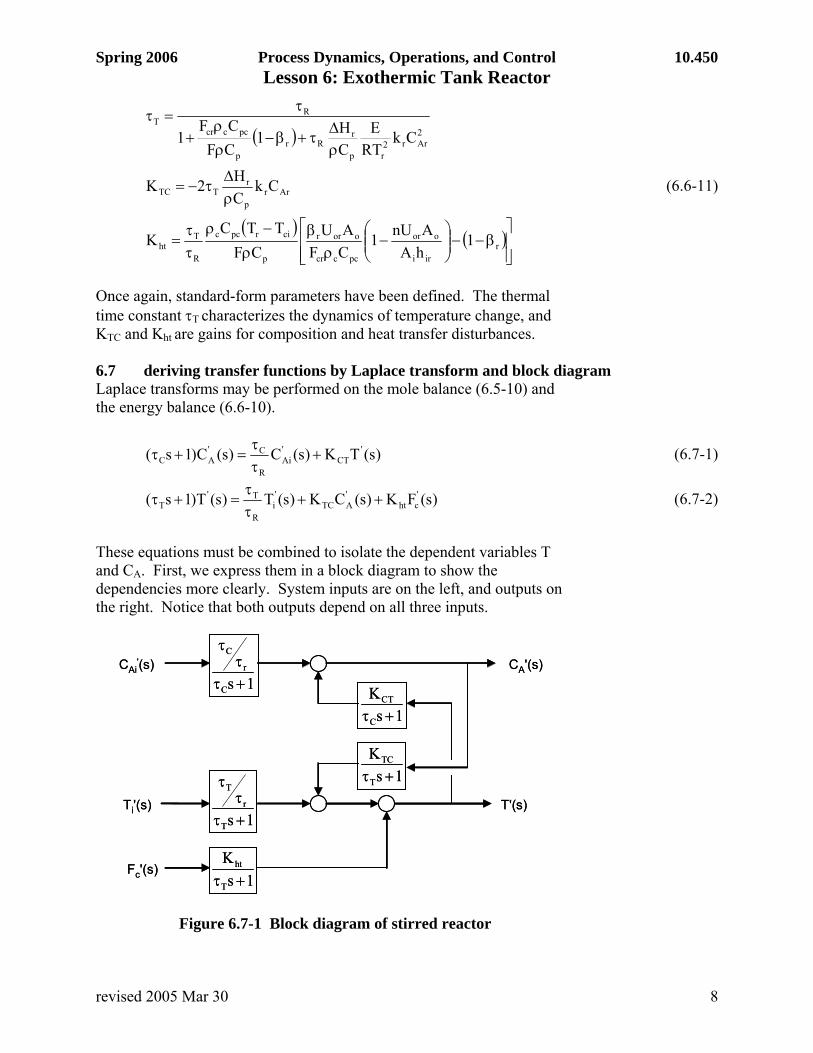
These equations must be combined to isolate the dependent variables T and CA. First, we express them in a block diagram to show the dependencies more clearly. System inputs are on the left, and outputs on the right. Notice that both outputs depend on all three inputs.
CAi'(s)
1sC
r
C
+ττ
τCA'(s)
1sK
C
CT
+τ
1sK
T
TC
+τ
1sT
r
T
+ττ
τ
1sK
T
ht
+τ
Ti'(s)
Fc'(s)
T'(s)
CAi'(s)
1sC
r
C
+ττ
τCA'(s)
1sK
C
CT
+τ
1sK
T
TC
+τ
1sT
r
T
+ττ
τ
1sK
T
ht
+τ
Ti'(s)
Fc'(s)
T'(s)
Figure 6.7-1 Block diagram of stirred reactor
revised 2005 Mar 30 8
Spring 2006 Process Dynamics, Operations, and Control 10.450 Lesson 6: Exothermic Tank Reactor We isolate CA
′(s) either by eliminating T′(s) between (6.7-1) and (6.7-2), or by tracing the dependency through the block diagram:
( )
( )( )
( )( )
( )( )
( )( )
( )( ))s(F
1s1sKK1
1s1sKK
)s(T
1s1sKK1
1s1sK
)s(C
1s1sKK1
1s)s(C 'c
TC
TCCT
TC
htCT
'i
TC
TCCT
TCR
TCT
'Ai
TC
TCCT
CR
C
'A
+τ+τ−
+τ+τ+
+τ+τ−
+τ+τττ
+
+τ+τ−
+τττ
= (6.7-3)
After simplifying the individual transfer functions in (6.7-3), we recognize a second-order system
( ))s(F
1s2s
KK
)s(T1s2s
K
)s(C1s2s
1s)s(C '
c22CT
htCT2
'i22
CR
CT2
'Ai22
TTR
2
'A +τξ+τ
τττ
++τξ+τ
τττ
++τξ+τ
+ττττ
= (6.7-4)
in which the coefficients in the characteristic equation are
TCCT
TC2
KK1−ττ
=τ (6.7-5)
TCCT
TC
KK12
−τ+τ
=τξ (6.7-6)
We similarly isolate T′(s) from the equations or the diagram to find
( ) ( ))s(F
1s2s
1sK
)s(C1s2s
K
)s(T1s2s
1s)s(T '
c22
CTC
ht2
'Ai22
TR
TC2
'i22
CCR
2
'
+τξ+τ
+τττ
τ
++τξ+τ
τττ
++τξ+τ
+ττττ
= (6.7-7)
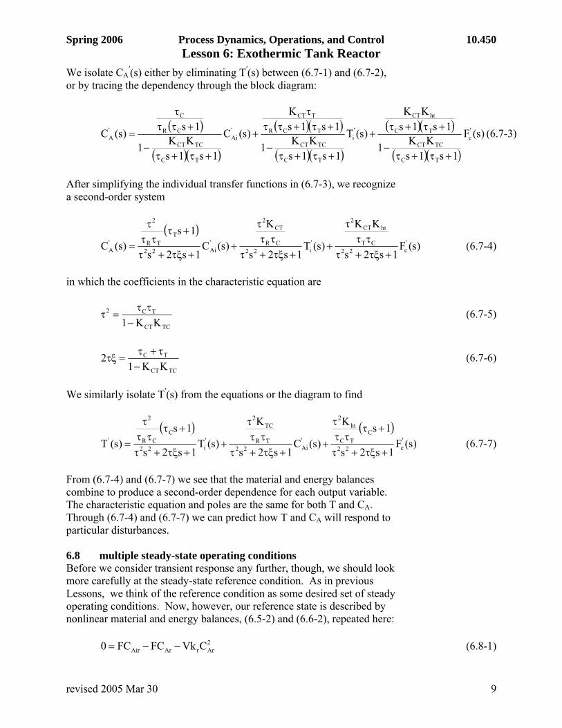
From (6.7-4) and (6.7-7) we see that the material and energy balances combine to produce a second-order dependence for each output variable. The characteristic equation and poles are the same for both T and CA. Through (6.7-4) and (6.7-7) we can predict how T and CA will respond to particular disturbances. 6.8 multiple steady-state operating conditions Before we consider transient response any further, though, we should look more carefully at the steady-state reference condition. As in previous Lessons, we think of the reference condition as some desired set of steady operating conditions. Now, however, our reference state is described by nonlinear material and energy balances, (6.5-2) and (6.6-2), repeated here:
2ArrArAir CVkFCFC0 −−= (6.8-1)
revised 2005 Mar 30 9
Spring 2006 Process Dynamics, Operations, and Control 10.450 Lesson 6: Exothermic Tank Reactor
( )( )rcirpcccr2ArrRrpirp 1TTCFCVkHTCFTCF0 β−−ρ−Δ−ρ−ρ= (6.8-2)
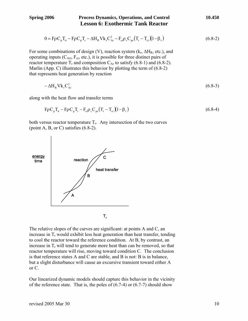
For some combinations of design (V), reaction system (kr, ΔHR, etc.), and operating inputs (CAir, Fcr, etc.), it is possible for three distinct pairs of reactor temperature Tr and composition CAr to satisfy (6.8-1) and (6.8-2). Marlin (App. C) illustrates this behavior by plotting the term of (6.8-2) that represents heat generation by reaction
2ArrR CVkHΔ− (6.8-3)
along with the heat flow and transfer terms
( )( )rcirpcccrrpirp 1TTCFTCFTCF β−−ρ−ρ−ρ (6.8-4) both versus reactor temperature Tr. Any intersection of the two curves (point A, B, or C) satisfies (6.8-2).
Tr
energytime
C
B
A
reaction
heat transfer
Tr
energytime
C
B
A
reaction
heat transfer
The relative slopes of the curves are significant: at points A and C, an increase in Tr would exhibit less heat generation than heat transfer, tending to cool the reactor toward the reference condition. At B, by contrast, an increase in Tr will tend to generate more heat than can be removed, so that reactor temperature will rise, moving toward condition C. The conclusion is that reference states A and C are stable, and B is not: B is in balance, but a slight disturbance will cause an excursive transient toward either A or C. Our linearized dynamic models should capture this behavior in the vicinity of the reference state. That is, the poles of (6.7-4) or (6.7-7) should show
revised 2005 Mar 30 10
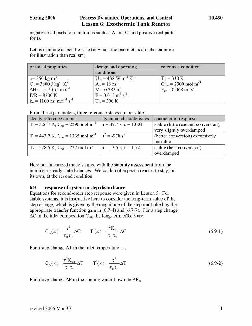
Spring 2006 Process Dynamics, Operations, and Control 10.450 Lesson 6: Exothermic Tank Reactor negative real parts for conditions such as A and C, and positive real parts for B. Let us examine a specific case (in which the parameters are chosen more for illustration than realism): physical properties design and operating
conditions reference conditions
ρ= 850 kg m-3 Cp = 3800 J kg-1 K-1 ΔHR = -450 kJ mol-1 E/R = 8200 K ko = 1100 m3 mol-1 s-1
Uor = 438 W m-2 K-1 Ao = 18 m2 V = 0.785 m3 F = 0.015 m3 s-1 Tci = 300 K
Tir = 330 K CAir = 2300 mol m-3 Fcr = 0.008 m3 s-1
From these parameters, three reference states are possible: steady reference output dynamic characteristics character of response Tr = 326.7 K, CAr = 2296 mol m-3 τ = 49.7 s, ξ = 1.001 stable (little reactant conversion),
very slightly overdamped Tr = 443.7 K, CAr = 1335 mol m-3 τ2 = -978 s2 (better conversion) excursively
unstable Tr = 578.5 K, CAr = 227 mol m-3 τ = 13.5 s, ξ = 1.72 stable (best conversion),
overdamped Here our linearized models agree with the stability assessment from the nonlinear steady state balances. We could not expect a reactor to stay, on its own, at the second condition. 6.9 response of system to step disturbance Equations for second-order step response were given in Lesson 5. For stable systems, it is instructive here to consider the long-term value of the step change, which is given by the magnitude of the step multiplied by the appropriate transfer function gain in (6.7-4) and (6.7-7). For a step change ΔC in the inlet composition CAi, the long-term effects are
CK)(TC)(CTR
TC2
'
TR
2'A Δ
τττ
=∞Δτττ
=∞ (6.9-1)
For a step change ΔT in the inlet temperature Ti,
T)(TTK)(CCR
2'
CR
CT2
'A Δ
τττ
=∞Δττ
τ=∞ (6.9-2)
For a step change ΔF in the cooling water flow rate ΔFc,
revised 2005 Mar 30 11
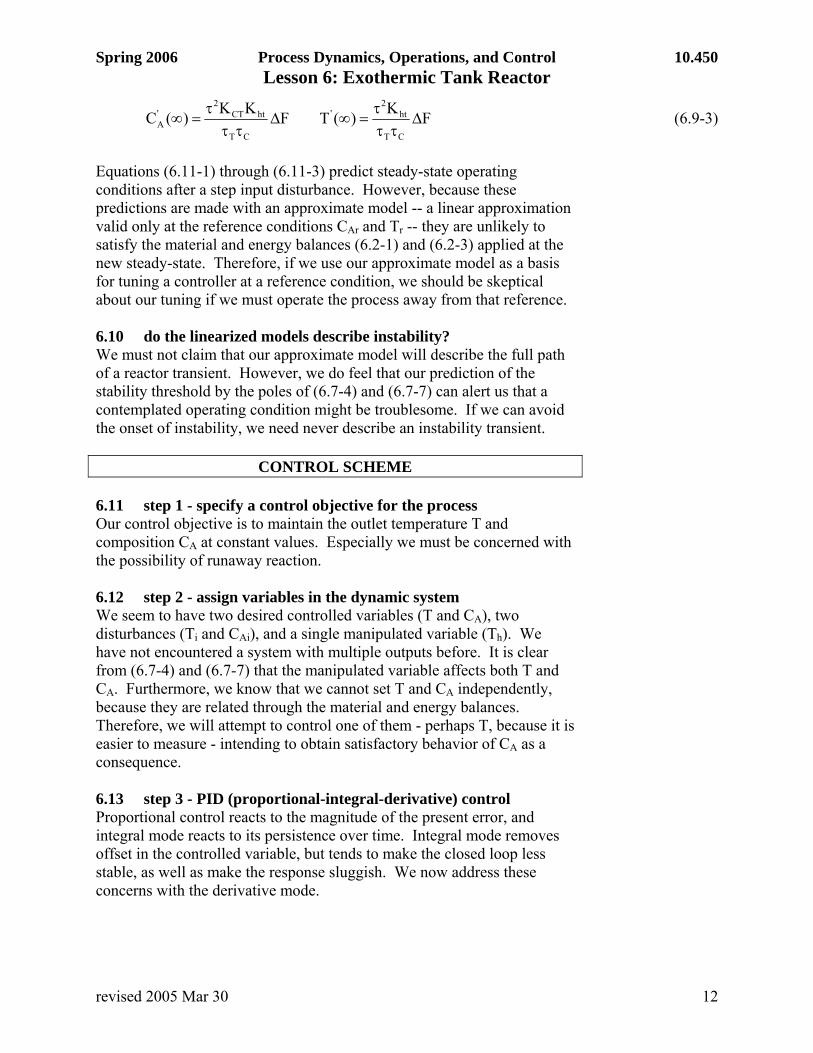
Spring 2006 Process Dynamics, Operations, and Control 10.450 Lesson 6: Exothermic Tank Reactor
FK)(TFKK)(CCT
ht2
'
CT
htCT2
'A Δ
τττ
=∞Δττ
τ=∞ (6.9-3)
Equations (6.11-1) through (6.11-3) predict steady-state operating conditions after a step input disturbance. However, because these predictions are made with an approximate model -- a linear approximation valid only at the reference conditions CAr and Tr -- they are unlikely to satisfy the material and energy balances (6.2-1) and (6.2-3) applied at the new steady-state. Therefore, if we use our approximate model as a basis for tuning a controller at a reference condition, we should be skeptical about our tuning if we must operate the process away from that reference. 6.10 do the linearized models describe instability? We must not claim that our approximate model will describe the full path of a reactor transient. However, we do feel that our prediction of the stability threshold by the poles of (6.7-4) and (6.7-7) can alert us that a contemplated operating condition might be troublesome. If we can avoid the onset of instability, we need never describe an instability transient.
CONTROL SCHEME 6.11 step 1 - specify a control objective for the process Our control objective is to maintain the outlet temperature T and composition CA at constant values. Especially we must be concerned with the possibility of runaway reaction. 6.12 step 2 - assign variables in the dynamic system We seem to have two desired controlled variables (T and CA), two disturbances (Ti and CAi), and a single manipulated variable (Th). We have not encountered a system with multiple outputs before. It is clear from (6.7-4) and (6.7-7) that the manipulated variable affects both T and CA. Furthermore, we know that we cannot set T and CA independently, because they are related through the material and energy balances. Therefore, we will attempt to control one of them - perhaps T, because it is easier to measure - intending to obtain satisfactory behavior of CA as a consequence. 6.13 step 3 - PID (proportional-integral-derivative) control Proportional control reacts to the magnitude of the present error, and integral mode reacts to its persistence over time. Integral mode removes offset in the controlled variable, but tends to make the closed loop less stable, as well as make the response sluggish. We now address these concerns with the derivative mode.
revised 2005 Mar 30 12
Spring 2006 Process Dynamics, Operations, and Control 10.450 Lesson 6: Exothermic Tank Reactor
⎟⎟⎠
⎞⎜⎜⎝
⎛ ε+ε+ε=− ∫ dt
dTdtT1Kxx
*
D
t
0
*
I
**c
*b,co
*co (6.13-1)
where x*
co is the controller output and the controlled variable error, expressed in scaled variables, is
**sp
* yy −=ε (6.13-2) Equation (6.13-1) describes the ideal PID (proportional-integral-derivative) controller algorithm. It adds the derivative mode to the proportional and integral modes we have seen before. Derivative mode is an early warning of error; by reacting to the change in the error signal, it can dictate a significant response from the manipulated variable before the error has grown sufficiently to evoke a similar response via proportional mode. The influence of the derivative mode is set by the magnitude of the derivative time TD. Increasing TD strengthens the controller response. We can express algorithm (6.13-1) in deviation variables.
⎟⎟⎠
⎞⎜⎜⎝
⎛ ε+ε+ε=
⎟⎟⎠
⎞⎜⎜⎝
⎛ ε+ε+ε
Δ=
∫
∫
dtdTdt
T1K
dtdTdt
T1
y%100Kx
D
t
0Ic
D
t
0I
*c
'co
(6.13-3)
The Laplace transform of (6.13-3) is
( ) ( ) ( )
( ))s(y)s(ysTsT
11K
)s(y)s(ysT)s(y)s(ysT
1)s(y)s(yK)s(x
''spD
Ic
''spD
''sp
I
''spc
'co
−⎟⎟⎠
⎞⎜⎜⎝
⎛++=
⎟⎟⎠
⎞⎜⎜⎝
⎛−+−+−=
(6.13-4)
6.14 step 4 - choose set points and limits Both the set point and operating limits for temperature may depend on a number of considerations, including reaction kinetics (desired reaction rate), reaction equilibrium (possible conversion), the possibility of side-products or degradation reactions, the vapor pressure of solvents, limits of construction materials, etc. Because our process may be open-loop unstable, we ask whether control can stabilize it.
EQUIPMENT
revised 2005 Mar 30 13
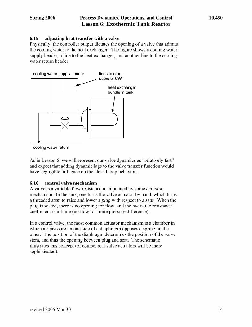
Spring 2006 Process Dynamics, Operations, and Control 10.450 Lesson 6: Exothermic Tank Reactor 6.15 adjusting heat transfer with a valve Physically, the controller output dictates the opening of a valve that admits the cooling water to the heat exchanger. The figure shows a cooling water supply header, a line to the heat exchanger, and another line to the cooling water return header.
cooling water supply header
cooling water return
heat exchanger bundle in tank
lines to other users of CW
cooling water supply header
cooling water return
heat exchanger bundle in tank
lines to other users of CW
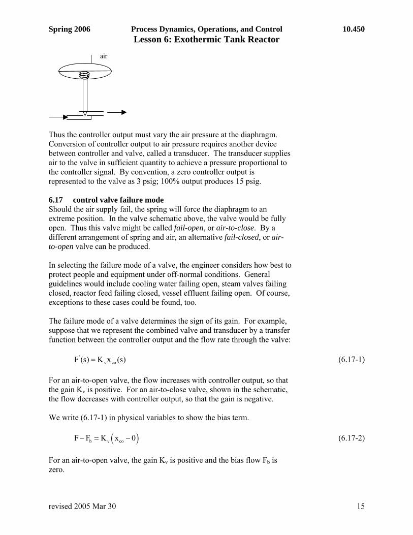
As in Lesson 5, we will represent our valve dynamics as “relatively fast” and expect that adding dynamic lags to the valve transfer function would have negligible influence on the closed loop behavior. 6.16 control valve mechanism A valve is a variable flow resistance manipulated by some actuator mechanism. In the sink, one turns the valve actuator by hand, which turns a threaded stem to raise and lower a plug with respect to a seat. When the plug is seated, there is no opening for flow, and the hydraulic resistance coefficient is infinite (no flow for finite pressure difference). In a control valve, the most common actuator mechanism is a chamber in which air pressure on one side of a diaphragm opposes a spring on the other. The position of the diaphragm determines the position of the valve stem, and thus the opening between plug and seat. The schematic illustrates this concept (of course, real valve actuators will be more sophisticated).
revised 2005 Mar 30 14
Spring 2006 Process Dynamics, Operations, and Control 10.450 Lesson 6: Exothermic Tank Reactor
air
Thus the controller output must vary the air pressure at the diaphragm. Conversion of controller output to air pressure requires another device between controller and valve, called a transducer. The transducer supplies air to the valve in sufficient quantity to achieve a pressure proportional to the controller signal. By convention, a zero controller output is represented to the valve as 3 psig; 100% output produces 15 psig. 6.17 control valve failure mode Should the air supply fail, the spring will force the diaphragm to an extreme position. In the valve schematic above, the valve would be fully open. Thus this valve might be called fail-open, or air-to-close. By a different arrangement of spring and air, an alternative fail-closed, or air-to-open valve can be produced. In selecting the failure mode of a valve, the engineer considers how best to protect people and equipment under off-normal conditions. General guidelines would include cooling water failing open, steam valves failing closed, reactor feed failing closed, vessel effluent failing open. Of course, exceptions to these cases could be found, too. The failure mode of a valve determines the sign of its gain. For example, suppose that we represent the combined valve and transducer by a transfer function between the controller output and the flow rate through the valve:
)s(xK)s(F 'cov
' = (6.17-1) For an air-to-open valve, the flow increases with controller output, so that the gain Kv is positive. For an air-to-close valve, shown in the schematic, the flow decreases with controller output, so that the gain is negative. We write (6.17-1) in physical variables to show the bias term.
(b v coF F K x 0− = − ) (6.17-2) For an air-to-open valve, the gain Kv is positive and the bias flow Fb is zero.
revised 2005 Mar 30 15
Spring 2006 Process Dynamics, Operations, and Control 10.450 Lesson 6: Exothermic Tank Reactor
maxco
FF100%
= x (6.17-3)
For an air-to-close valve, the gain is negative, and bias flow is the maximum flow.
(maxco
FF 100% x100%
= )− (6.17-4)
Equations (6.17-3 and 4) are suitable for use in simulator calculations. 6.18 positive closed loop gain and the sense of the controller In these lessons, we have occasionally checked the sign of the gain in our dynamic systems. Finding in Section 6.17 that an air-to-close valve necessarily has a negative gain motivates us to examine the gains in a closed feedback loop. As a basis, we want feedback to be negative. That is, if the controlled variable becomes too large, we want the feedback loop to reduce it. The alternative positive feedback will tend to increase the already-too-high controlled variable. A common example of positive feedback occurs when the output of a loudspeaker is fed back into a microphone, amplified, and delivered to the speaker - cover your ears! Because we have defined error to be the set point less the controlled variable, a high controlled variable gives a negative error. If this error is acted upon by a positive gain around the loop, the feedback to the controlled variable is negative. Hence we want a positive loop gain. The loop gain KL is the gain component of the loop transfer function GL(s). Thus, the loop gain is the product of the sensor, controller, valve, and manipulated variable (process) gains.
mvcsL KKKKK = (6.18-1) • Of these, the gain Ks for most sensors is positive - the mercury rises
with temperature. • The process gain Km is determined by the process itself - in these
lessons, it has typically been positive, such that an increase in manipulated variable causes an increase in the response variable. However, we might in principle run across an opposite case.
• The sign of the valve gain Kv is a function of a safety analysis, as discussed in Section 6.17.
• Because Km and Kv may be either positive or negative, and can be so for independent reasons, we must therefore reserve the ability to
revised 2005 Mar 30 16
Spring 2006 Process Dynamics, Operations, and Control 10.450 Lesson 6: Exothermic Tank Reactor
choose the sign of the controller gain Kc. This is done with the controller sense switch, which might be a physical switch on an analog controller, or an input value in software.
6.19 ambiguity! The adjectives “direct-acting” and “reverse-acting” are used with a controller to indicate the position of the sense switch. Alternative adjectives are “increase/increase” and “increase/decrease”. However, the adjectives are not consistently used! Hence, look at the controller carefully, and ensure that you know the algebraic sign of the gain.
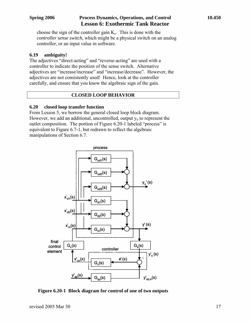
CLOSED LOOP BEHAVIOR 6.20 closed loop transfer function From Lesson 5, we borrow the general closed loop block diagram. However, we add an additional, uncontrolled, output yu to represent the outlet composition. The portion of Figure 6.20-1 labeled “process” is equivalent to Figure 6.7-1, but redrawn to reflect the algebraic manipulations of Section 6.7.
Gd2(s)
Gm(s)
Gs(s)
Gc(s)
Gv(s)
-
x'd2(s)
x'm(s) y' (s)
e' (s)x'co(s)
y'sp(s)
y's (s)
process
controller
final control element
Gsp(s) y'sp,s(s)
Gd1(s)x'
d1(s)
Gud2(s)
Gud3(s)
Gud1(s)
yu' (s)
Gd2(s)
Gm(s)
Gs(s)
Gc(s)
Gv(s)
-
x'd2(s)
x'm(s) y' (s)
e' (s)x'co(s)
y'sp(s)
y's (s)
process
controller
final control element
Gsp(s) y'sp,s(s)
Gd1(s)x'
d1(s)
Gud2(s)
Gud3(s)
Gud1(s)
yu' (s)
Figure 6.20-1 Block diagram for control of one of two outputs
revised 2005 Mar 30 17
Spring 2006 Process Dynamics, Operations, and Control 10.450 Lesson 6: Exothermic Tank Reactor Also from Lesson 5, the controlled variable is related to the inputs by
( ) ( ) ( ) )s(yGGGG1
GGGG)s(x
GGGG1G)s(x
GGGG1G)s(y '
spscvm
spcvm'2d
scvm
2d'1d
scvm
1d'
++
++
+= (6.20-1)
We specialize the nomenclature and the transfer functions for our stirred reactor case, using especially temperature model (6.7-7).
( )
1s2s
1s)s(G
)s(T)s(x
22
CCR
2
1d
'i
'1d
+τξ+τ
+ττττ
=
=
(6.20-2)
1s2s
K
)s(G
)s(C)s(x
22TR
TC2
2d
'Ai
'2d
+τξ+τττ
τ
=
=
(6.20-3)
( )
1s2s
1sK
)s(G
)s(F)s(x
22
CTC
ht2
m
'c
'm
+τξ+τ
+τττ
τ
=
=
(6.20-4)
)s(T)s(y
sTsT
11K)s(G
K)s(G)s(GK)s(G
''
DI
cc
sspsvv
=
⎟⎟⎠
⎞⎜⎜⎝
⎛++=
===
(6.20-5)
Motivated by Section 6.18, let us examine the loop gain: • The sensor gain Ks is positive for temperature measurement. • The process gain Km is given in (6.20-4). For a stable process, τ2, τC,
and Kht are all positive, but τT is negative. Hence, Km is negative, implying that an increase in the heat exchanger coolant flow will lower the reactor operating temperature.
• Because we wish to provide cooling water even in the event of an air supply failure, we choose an air-to-close valve. In Section 6.19, we saw that such a valve featured a negative gain.
• Because the product of the other three gain components is positive, our controller sense must be set to positive gain. If the reactor is too cold,
revised 2005 Mar 30 18
Spring 2006 Process Dynamics, Operations, and Control 10.450 Lesson 6: Exothermic Tank Reactor
T < Tsp and ε > 0. Positive Kc directs the controller output to increase, closing the air-to-close valve, restricting the cooling water, and thus allowing T to rise.
6.21 closed-loop behavior - laplace transform solution From the equations in Section 6.20, we can derive the transfer function for disturbances in the inlet temperature:
( )
⎪⎪
⎭
⎪⎪
⎬
⎫
⎪⎪
⎩
⎪⎪
⎨
⎧
+⎟⎟⎠
⎞⎜⎜⎝
⎛+
τ+
ττ
τ+
⎟⎟⎠
⎞⎜⎜⎝
⎛+
τ+
τξτ
τ+⎟⎟⎠
⎞⎜⎜⎝
⎛+
ττ
+ττ
τ
=
IIChtscv2
TC
2
C
D
htscv
TC
3D
htscv
TC
CThscvR
T
'i
'
T1s
T11
KKKK
s1TKKKK
2sTKKKK
s1sKKKK
)s(T)s(T (6.21-1)
The closed loop characteristic equation is third order, because the integral mode has increased the process order by one. Partial fraction expansion will show us that the step response will be the sum of three exponential terms (for 3 real roots) or an exponential oscillation (for 1 real and 2 complex roots). We could proceed as in Lesson 4, in which we calculated poles numerically and found the onset of oscillation, and then instability with increasing gain. Here our tuning task would be more complicated, because we have three controller parameters to vary, instead of just the gain. The derivative mode affects the coefficients of the two higher order terms. Increasing D will increase the curvature of the characteristic function, which (other parameters unchanged) can increase the likelihood of three abscissa-crossings - thus three real roots, suppressing oscillation in the response. The integral mode affects the lower order terms. Increasing TI will result ultimately in reducing the order of the characteristic equation, which will allow offset in the step response. Increasing the controller gain Kc will reduce the transfer function gain (the coefficient in the numerator) and reduce the magnitude of the dynamic term coefficients in the denominator. 6.22 Bode criterion for closed loop stability We invoke the Bode stability criterion, as we did in Lesson 4, with one important provision: the Bode criterion does not apply if the process is open-loop unstable. Therefore, if we are attempting to operate at such a condition, we must use more advanced methods to determine the closed-loop stability limits.
revised 2005 Mar 30 19
Spring 2006 Process Dynamics, Operations, and Control 10.450 Lesson 6: Exothermic Tank Reactor For stable open-loop conditions, we may apply the Bode criterion to the loop transfer function. The amplitude ratio is the magnitude of the loop transfer function, which may be found as the product of the magnitudes of the component transfer functions. Using a table of amplitude ratios, such as that of Marlin (2000), we find
( )( ) ( )2222
2C
TC
ht2
v
2
IDcsA
21
1KKT1T1KKR
τξω+ωτ−
ωτ+ττ
τ⎟⎟⎠
⎞⎜⎜⎝
⎛ω
−ω+= (6.22-1)
Similarly, the phase angle is the sum of the component phase angles.
( ) ⎟⎠⎞
⎜⎝⎛
ωτ−τξω−
+ωτ+⎟⎟⎠
⎞⎜⎜⎝
⎛ω
−ω=φ −−−22
1C
1
ID
1
12tantan
T1Ttan (6.22-2)
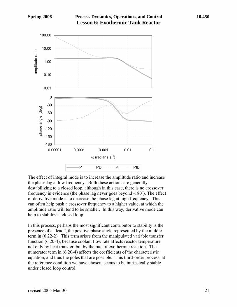
The derivative mode opposes the phase lag due to the integral mode and stabilizes the closed loop. In the figure, the controller parameters are set to give P, PD, PI, and PID controllers at a stable open-loop condition, as described in Section 6.8. Controllers using integral mode are shown with dashed lines; solid lines refer to P and PD controllers.
revised 2005 Mar 30 20
Spring 2006 Process Dynamics, Operations, and Control 10.450 Lesson 6: Exothermic Tank Reactor
0.01
0.10
1.00
10.00
100.00
0.00001 0.0001 0.001 0.01 0.1
ampl
itude
ratio
-180
-150
-120
-90
-60
-30
0
0.00001 0.0001 0.001 0.01 0.1
ω (radians s-1)
phas
e an
gle
(deg
)
P PD PI PID
0.01
0.10
1.00
10.00
100.00
0.00001 0.0001 0.001 0.01 0.1
ampl
itude
ratio
-180
-150
-120
-90
-60
-30
0
0.00001 0.0001 0.001 0.01 0.1
ω (radians s-1)
phas
e an
gle
(deg
)
P PD PI PID
The effect of integral mode is to increase the amplitude ratio and increase the phase lag at low frequency. Both these actions are generally destabilizing to a closed loop, although in this case, there is no crossover frequency in evidence (the phase lag never goes beyond -180º). The effect of derivative mode is to decrease the phase lag at high frequency. This can often help push a crossover frequency to a higher value, at which the amplitude ratio will tend to be smaller. In this way, derivative mode can help to stabilize a closed loop. In this process, perhaps the most significant contributor to stability is the presence of a “lead”, the positive phase angle represented by the middle term in (6.22-2). This term arises from the manipulated variable transfer function (6.20-4), because coolant flow rate affects reactor temperature not only by heat transfer, but by the rate of exothermic reaction. The numerator term in (6.20-4) affects the coefficients of the characteristic equation, and thus the poles that are possible. This third-order process, at the reference condition we have chosen, seems to be intrinsically stable under closed loop control.
revised 2005 Mar 30 21
Spring 2006 Process Dynamics, Operations, and Control 10.450 Lesson 6: Exothermic Tank Reactor 6.23 tuning the controller Given the process model, we may tune the controller by simulation, in which we vary the three parameters and assess the effects by comparing IE and IAE for the responses. The simulation can be done by supplying the partial fraction expressions with numerically computed roots, or by returning to the differential equations for numerical solution, either in linearized or original nonlinear form. 6.24 conclusion We encountered a more complicated process in this lesson, both because it required two coupled equations, and because reaction kinetics and heat transfer made them nonlinear. We introduced a formal approximation process to make the model linear, and then were able to treat it with tools we had previously developed. Even so, nonlinearity could not be escaped, because we found that the behavior of the approximate description depended on the reference conditions we chose. Furthermore, we found that some conditions admitted multiple steady states. All of this should inspire us to maintain a healthy skepticism toward our results. The positive news was that it is possible to maintain the process at an inherently unstable condition through feedback control. We have further increased our feedback capabilities through the derivative mode, which complements proportional and integral modes to comprise the PID controller, widely used and justly respected in the chemical process industries. 6.25 references Incropera, Frank P., and David P. DeWitt. Fundamentals of Heat and Mass Transfer.5th ed. New York, NY: J. Wiley, 2002. ISBN: 0471386502. Marlin, Thomas E. Process Control. 2nd ed. Boston, MA: McGraw-Hill, 2000.ISBN: 0070393621.
revised 2005 Mar 30 22