(. a revised national hurricane center€¦ · a revised national hurricane center nhc83 model...

f { !.JC~

~ 99:=;=i ~ ' R~ . '(ii 4 ~~ . ' 16 -"",..::.

I Property of no. 44 .",'ItIf NOM Coral Gables Library ,

~ Gab!es Olie Tower! 1320 South Dixie Highway, Room 520i Coral Gables, Florida 33145

jii NOAA Technical Memorandum NWS NHC-44

-t

I;,,"1:cJ

f(. A REVISED NATIONAL HURRICANE CENTER

"'; NHCS3 MODEL (NHC90)

.;

:,

i' ~

Prepared by: j

~ Charles J. Neumann 1'" Science Applications International Corporation :1'

": Contract No. 50DSNC-S-OO141 if i

.and:,

I .. Colin J. McAdle j

..: National Hurricane Center :I:

,-' 1, a i

~~Iir National Hurricane Centeri:#' i~ Coral Gables, Flonda 8 3 9 '[

r: "November 1991

11 ;Ir :"

, ~~ ISTATES National OceaDX: and AtmOSpberK: A~ National Weather ServK:e f~~ J

)PJ'ARTMENT OF COMMERCE John A. KDauss E]bert W. Friday "1 §~ A. Mosbacher, ~Nary Under ~retary and AdminQrator Assistant Administrator '-..~ ...i"" I: ~~~ .'J f

..

f,i .'

*!:

::;~'"t TABLE OF CONTENTS

~..:if

~,,!I' Abstract 1 Hf.i: ;':, 1. Background 1 I

~ 1.1 Tropical cyclone prediction models. 1"~" 1. 1. 1 Introduction. 1 I

1.1.2 Types of motion models. 1 ~1.1.3 Statistical-dynamical models. 2 ~1 .2 The NHC83 model. 21.2.1 Performance of NHC83. 2 ~b . d ? 4 ;1 .2 .2 Can NHC83 e J.mprove :11.3 Purpose of study. 4 ~

~ M': 2. Model deficiencies. 4 ~i

2.1 Non-correctable (external) deficiencies. 52.1.1 Reliance on numerical guidance. 52.1.2 Initial motion vectors. 72.2 Partially correctable (external) deficiencies. 7 ;:2.2.1 Initial analyses problems. 72.2.2 Bias in numerical forecasts. 92.3 Correctable deficiencies. 102.3.1 Inconsistencies in NHC83 forecast track. 10 ."

2.3.2 Inconsistencies in NHC83 stratification scheme. ..10 :2.3.3 Geographical limitations in development data. ...11 i2.3.4 Predictor selection logic. 11 :2 .3 .5 Graphical output. 12 ;2.4 Summary of differences between NHC83 and NHC90 12 :

3. Development of the NHC90 model. 12 :3 .1 Introduction. 12 -I.3.2 Developmental data. 13 ,"3 .2 .1 Sample size. 133.2.2 stratification. 133.2.3 statistical attributes of development data. 143.2.4 Composite analyses. 153.3 Selection of predictors. 173.3.1 Analysis mode vs. perfect-prog mode. 173.3.2 Selection criteria. 17 ~3.3.3 Pairing of predictors. 183.3.4 Example of predictor selection, North Zone, along it

track. 18 I3.3.5 Examples of predictor selection, North Zone, acrosstrack. 20 ,

3.3.6 Example of predictor selection, South Zone, along"track. 20

3.3.7 Final selection of predictors. 20 j

iI

f;

t

, "' .'", _.."~. "

II '

1' , .: ;

f

J4. Model performance on development data. 23 14.1 Reductions of variance. 23 ~4.1.1 Review of model structure. 23 ,4.1.2 Comparison of variance reductions. 23 I4.2 Forecast error. 27 ;

I5. Graphics packa~e. 29 t5.1 NHC83 graph1cs package. 29 I5.2 NHC90 graphics package. 29 I

6. Potential for additional improvement to NHC90 306. 1 Grid rotation. 306.1.1 The NHC83/NHC90 system. 30

: 6.1.2 Proposed NHC90 grid rotation system. 30I 6.2 Use of winds rather than heights. 33

7 .References 34 1

I

,I,, i

II

Iti

;

IiJ I

I

j!

,

"I"1 ....,,-"~. ",,' _".0. ._~ " c "...,_._w.~.O"~,

"

.'

A REVISED NATIONAL HURRICANE CENTER NHC83 MODEL (NHC90) ,

fi"Charles J. Neumann :Science- Applications International Corporation1 ~

Ii Colin J. McAdie! National Hurricane Center

ABSTRACT

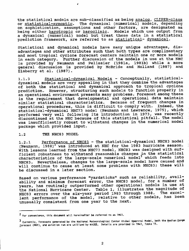
I--The National Hurricane Center (NHC) statistical-dynamical NHC83 model was introduced 'Iopera_tio~ally for t~e 1?~ hurricane season. Based on a number of evaluation criteria such Ias tImelIness, avaIlabILIty, overall utility and minimum error, NHC83, through the 1988hurricane season, has outperformed other models in use at NHC by a rather wide margin. .'Accordingly, this type of prediction model appears to be very sound. Nevertheless, long-termoperational use of the model has disclosed certain design weaknesses. These are reviewed.The question is posed as to the potential for still further improvement to NHC83 by addressingand correcting these deficiencies.

Two approaches to potential improvement are suggested. The first involves maintaining thebasic integrity of the model but using deep-layer-mean winds rather than deep-layer-mean ::geopotential heights as the main source of predictive information. The second method involves r~retaining the geopotential heights as predictors but revising the model based upon an ,:evaluation of NHC83 1983-1988 error patterns. N

Each method appeared to have cons i derabl e meri t and both were undertaken. Th i s study reportson a revision to the model using the second of the two approaches; that is, maintaining theheight fields but addressing identifiable deficiencies. Forecast errors obtained fromdevelopmental data, when compared to those of the original NHC83 model, suggest that the newmodel (NHC90) should outperform NHC83. However, this must still be confirmed through one ormore years of operational testing.

The other approach, that is, revising the model using deep-layer-mean winds rather thanheights, is still under development and is discussed briefly in Section 6.

1. BACKGROUND !

1.1 TROPICAL CYCLONE PREDICTION MODELS

1.1.1 IntroductioB -Preparatory to the issuance of tropicalcyclone advisories, the National Hurricane Center (NHC) activates anumber of models which provide objective guidance on various aspectsof tropical cyclone prediction. Essentially, these models fall into

three categories: those for the prediction of (1) tropical cyclone

motion, (2) tropical cyclone intensity and (3) storm surge. Effortsare continually underway at NHC and elsewhere to improve on the per-formance of these models. This study reports on recent and proposedimprovements to the NHC83 model, one of the principal NHC models forguidance on tropical cyclone motion.

1.1.2 ~es gf Mot~on Model§ -In the broadest sense, models forthe prediction of tropical cyclone motion can be classified as being Jeither statistical or dynamical (numerical). Depending on the method,of treating developmental data and the type of predictors employed, ,

1 Prepared for the National Hurricane Center, Coral Gables, FL 33146: Contract Number 50DSNC-8-00141. Contract

partially supported by NOAA/ERL AOML-Hurricane Research Division (HRD).

1 l

I--

..ill".~,

.'

the statistical models are sub-classified as being analoq, CLIPER-classor stat~st~cal~synoPtic. T?e dynamical (numerical) models, dependingon soph1st1cat1on, assumpt1ons and other factors, are designated as

: being either barotro~ic or baroclinic. Models which use output from" a dynamical (numerical) model but treat these data in a statistical~ prediction framework, are referred to as statistical- dynamical.

statistical and dynamical models have many unique advantages, dis-~j advantages and other attributes such that both types are complimentary, ~nd most tropical cyclone fo~ecast .centers maintain o~e or more models

1n each category. Further d1scuss1on of the models 1n use at the NHC,', is provided by Neumann and Pelissier (1981a, 1981b) while a more) general discussion is provided by McBride and Holland (1987) and

I Elsberry et ale (1987).I

1.1.3 statistical-dvnamical Models -conceptually, statistical-dynamical models are very appealing in that they combine the advantagesof both the statistical and dynamical approach to tropical cyclone

"' prediction. However, structuring such models to function properly inan operational environment presents many problems. Foremost among theseis the requirement that developmental and operational data maintainsimilar statistical characteristics. Because of frequent changes inoperational procedures, this is difficult to comply with. Indeed, thestatistical-dynamical NHC73 model (Neumann and Lawrence, 1975), whichperformed very well following its introduction in 1973, was recentlydiscontinued at the NHC because of this statistical pitfall. The modelwas insufficiently robust to withstand changes in the numerical modelpackage which provided input.

1 .2 THE NHC83 MODEL

1.2.1 Performance of NHC83 -The statistical-dynamical NHC83 model(Neumann, -i9-88)~ was introduced at NHC for the 1983 hurricane season.

I with lessons learned from the NHC73 model, NHC83 was designed with suf-ficient robustness to withstand reasonable changes in the statisticalcharacteristics of the large-scale numerical model3 which feeds intoNHC83. Nevertheless, changes to the large-scale model have caused andwill continue to cause at least some problems with NHC83; these willbe discussed in a later section.

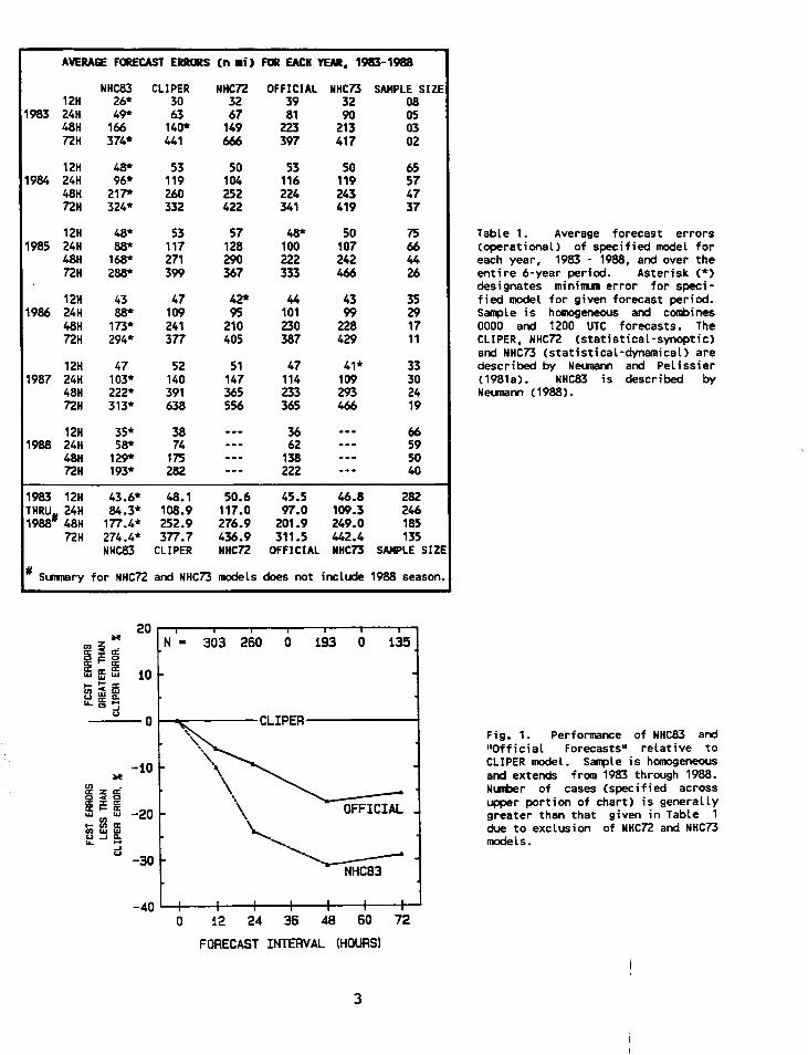
Based on various performance "yardsticks" such as reliability, avail-ability and minimum forecast error, the NHC83 model, for a number ofyears, has routinely outperformed other operational models in use atthe National Hurricane Center. Table 1, illustrates the magnitude ofNHC83 errors over the six-year period 1983 through 1988. The excel-lent performance of the model, relative to other models, has beenunusually consistent from one year to the next.

2 For convenience, this document will hereinafter be referred to as TM41.

3 Currently, forecasts generated by the National Meteorological Center Global Spectral Model, both the ~edium Rangeforecast (MRF), and aviation run are utilized by NHC83. Details are provided in TM41, Table 11.

2

L ~ ~".".~~"".~".~_.,~ "'

.~

AVERAGE F~CAST E~S (n .i) F~ EACH YEAR, 1983-1988

NHC83 CLIPER NHC72 OFFICIAL NHC73 SAMPLE SIZE :12H 26* 30 32 39 32 08 II

1983 24H 49* 63 67 81 90 05~"

48H 166 140* 149 223 213 0372H 374* 441 666 397 417 02 t.

12H 48* 53 50 53 50 65 f1984 24H 96* 119 104 116 119 57 f

48H 217* 260 252 224 243 4772H 324* 332 422 341 419 37 ,1.

:!12H 48* 53 57 48* 50 75 Table 1. Average forecast errors .

1985 24H 88* 117 128 100 107 66 (operational) of specified model for I;

48H 168* 271 290 222 242 44 each year, 1983 -1988, and over the72H 288* 399 367 333 466 26 entire 6-year period. AsterisK (*)

designates minimum error for speci-12H 43 47 42* 44 43 35 fied model for given forecast period.

I,1986 24H 88* 109 95 101 99 29 Sample is homogeneous and combines

48H 173* 241 210 230 228 17 0000 and 1200 UTC forecasts. The72H 294* 377 405 387 429 11 CLIPER, NHC72 (statistical-synoptic) ~

and NHC73 (statistical-dynamical) are12H 47 52 51 47 41* 33 described by Neumann and Pelissier

1987 24H 103* 140 147 114 109 30 (1981a). NHC83 is described by "48H 222* 391 365 233 293 24 Neumam (1988). .

72H 313* 638 556 365 466 19

12H 35* 38 ---36 ---661988 24H 58* 74 ---62 ---59

48H 129* 175 ---138 ---5072H 193* 282 ---222 ---40

1983 12H 43.6* 48.1 50.6 45.5 46.8 282THRU 24H 84.3* 108.9 117.0 97.0 109.3 2461988# 48H 177.4* 252.9 276.9 201.9 249.0 185

72H 274.4* 377.7 436.9 311.5 442.4 135NHC83 CLIPER NHC72 OFFICIAL NHC73 SAMPLE SIZE

# Summary for NHC72 and NHC73 models does not include 1988 season. 1

20~ z ~ N -303 260 0 193 0 135a:ca::o~oI-~ ~ ~ 10"'",'"I-I-~~c",,,"'Q.II-a:...m-,

"0 CUPER" Fig. 1. Performance of NHC83 and ;1

" "Official Forecasts" relative to 1-10 " CLIPER model. Sample i s homogeneous I~ \, and extends from 1983 through 1988.

~ z a::', Number of cases (specified across~ ~ g ", upper portion of chart) is generally"': ffi -20 " OFFICIAL greater than that given in Table 1 .

;j", fi ~ ~ \ due to exclusion of NHC72 and NHC73II- ~ '... models. .,.., " "- ;

" -30 ~--,:,- NHC83 ~

: -40 0 12 24 36 48 60 72 1

.FORECAST INTERVAL (HOURS)"'"t'"t 3

6' J

" I

One of the advantages of NHC83 is the excellent performance at theimportant 24 h projection. This is demonstrated in Fig. 1 where arapid improvement over climatology and persistence (CLIPER), 0 through24 h (and beyond) is evident. This can be attributed to: (1) largescale "steering" information contained in the National MeteorologicalCenter (NMC) Global Spectral Model used by NHC83, (2) NHC83methodology used in extracting this information and (3) the NHC83rotated grid system (Shapiro and Neumann, 1984).

1.2.2 Can NHC83 be imDroved? -The predictive skill of NHC83 isobtained from forecast deep-layer-mean geopotential height fieldsderived from various runs of the NMC global spectral model (seefootnote 3).

Given the excellent performance of NHC83, further improvement mightnot seem necessary; however, close monitoring of forecasts from themodel during the period, 1983-1988, disclosed several design weak-nesses which were amenable to correction. Additionally, the currentNHC83 model was developed from an analysis domain which did not ex-tend into the deep tropics; a more recent developmental data set couldtake full advantage of a larger grid domain extending further into thetropics.

Another possible approach to improvement was to abandon the use ofgeopotential heights entirely in favor of deep-layer-mean winds. Apreliminary exploration of this approach is discussed by Pike (1987a).

Thus, there are two broad-scale approaches to potential improvementsin the NHC83 model: (1) continue using geopotential heights as pre-dictors, correct identifiable weaknesses and gain the advantage ofusing an updated developmental data set, or (2) use deep-layer-meanwinds as input, based on preliminary evidence that their use resultsin a reduction in track forecast errors. In either of the twoapproaches, the basic structure of the present NHC83 model would notbe changed.

1. 3 PURPOSE OF STUDY

This report addresses the first of the above two proposals. Thei essential purpose of the report is to provide documentation for this! revised NHC83 model, to be known as NHC90. Work has also been

accomplished on approach (2) but is only briefly addressed in the finalsection.

2. MODEL DEFICIENCIESiI

; Close monitoring of NHC83 over the past several years and recent eval-i uations of the error characteristics have disclosed several internal, i weaknesses in model structure. Some of these weaknesses can be

addressed and corrected while others must be considered as inherent! deficiencies in this type of model or external to NHC83 and not being

correctable. still other external deficiencies can be at leastpartially alleviated.

4

,

III'"III." 1 FORECAST PERIOD. 72 MaRS

~ SAMPLE SIZE. !70~ AVERAGE EI¥IOA .277.6 N.M!.~ 0 STIiJ DEVN OF ~ .162.3 N.M!."~'"c-

oo000000000000000000000000000000000

~~~N~~-~-O~~~N~~-~-O~~~N~~-~-O~~---NNN~~~~~~~~~~~~~~~~~~~m~~~

FIllECAST ~ IN NAUTICAL MILS

~ 11 ,~ :" 1 FORECAST PERIOO .~8 H~

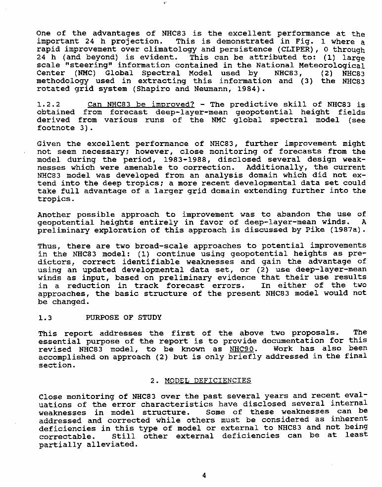
is SAIG'LE SIZE. 228 Fig. 2. Frequency distribution~ AVERA6E ~ .180.9 N.Ml. f NHC83 I l 24 48 -..I 72h~ 0 STND DEVN IF E;RDRS -!21.1 N.M1. 0 \I~e, ar~

~ forecast errors over 6-year~ period, 1983-1988. I

00000000000000000000000000000000000

~~~N~~-~~O~~~N~m-~~O~~~N~m-~~o~~---NNN~~~~~~~~~~~~~~~~~~mm~~~

F~CAST EIiIM IN NAUTICAL MILS

1 :~

III

5 10 FIllECAST PERIOD -2~ H(J.JIS ~is SAWLE SIZE. 302 !

~ AVERA6E EIiIM. 87.~ N,M!. :~ 05 S~ DEVN IF ~. 59.5 N.M1."~~

00000000000000000000000000000000000

~~~N~m-~~O~=~N~=-~~O~=~N~m-~~o~~---NNN~~~~~~~~~~===~~~~mmm~~~

FIllECAST ERIm IN NAUTICAL MILS

"

':

2.1 NON-CORRECTABLE (EXTERNAL) DEFICIENCIES 1

2.1.1 Reliance on Numerical Guidance -Fig. 2 is a frequencydistribution of NHC83 operational forecast errors. Comparing theseerrors to those of other statistical models discloses that NHC83 makesfewer "large" forecast errors. Indeed, this is one of the reasons thatthe overall forecast error of NHC83 is comparatively low. Since NHC83forecasts are explicitly tied to output from the NMC Global SpectralModel (Extended 240h run, Aviation Run or Global Data Assimilation 1Run), this attests to the skill of the latter in projecting the large- Iscale steering flow and related NHC83 skill in extracting this j..information. There is apparently more statistical predictiveinformation contained in these numerical prognoses than previously:thought available. j,Nevertheless, as shown in Fig. 2, occasional large errors, defined here l

as the mean plus 2 standard deviations, do occur. An analysis of the "larger errors shows that they are typically caused by poor prognosesof the large-scale steering patterns. The largest 72 h error, for 1

example (933 n mi on Hurricane Josephine, initial UTC 84101512),occurred when the Global Spectral Model mispositioned a large cold-low jover the North Atlantic. In that NHC83 is explicitly tied to this

"numerical output, there is no practical way to avoid these occasional,poor forecasts.

4 .'Since the NHC83 model was developed in the "Perfect-Frog" mode, thJ.S Jprovides a convenient method for separating the effect of errors in ':

II

i4 "Perfect-Prog: refers to the use of observed, rather than forecast fields in the Ioodel develo!Jllent phase. :

t5 ., ri '

1

t;

..!I

12 55 ;~ 5 j

~ 0

3 5.0

2 25.2 20,I IS

I 10

I \5.t I 1

0 / 0

123.5120 115 110 105 100 95 90 85 80 75 ~ ~ 20 15 10 5

NATIONAL HURRICANE CENTER. MIAMI. FL DEEP-LAYER-MEAN 80091700SEP 17 1980 aOODGMT 33.0N ~8.0W 038/13 90KTS FRANCIS

Ii

80 75 ~O 35 3D 25 20 5

0

5

0

5

! 0

II 5

0i

---, ' ..., 0 ~ 0

123.5120 115 110 IDS 100 95 90 85 80 75 5

NATIONAL HURRICANE CENTER. MIAMI. FL DEEP-LAYER-MEAN 80080300AUG 3 1980 aOOOGMT 12.~N Si.~W 27~/22 6SKTS ALLEN

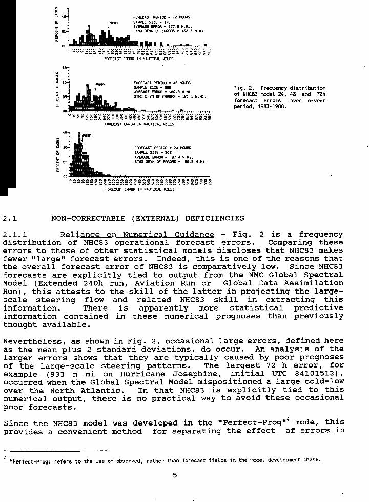
Fig. 3a. (top) and 3b. (bottom) showing examples of initial deep-Layer-mean wind and geopotentiaL heightanalyses where tropical cyclone vortex is not present. Upper chart is for a case after storm recurvature

0 into the westerlies, while lower chart is before recurvature. Center of tropical cyclone (obtained frombest-track of storm) is identified by darkened hurricane symbol. Heights are in meters; standard heightof deep-Layer-mean field is 6060.5 meters. Winds, in knots, are plotted at standard NMC grid points.

j Information below chart includes storm position, instantaneous motion (degs/knots) and maximum surfaceft wind (knots) within storm at current time.

j

!10,

l 6

I. i.

'C"O'~oO'~.c" '"oC"'~~"C.c".~".c .,~, "".~"-""-"'~C

.

:ii 1 80

5

I aI

5

a

5

0

5

0

5

a5

NATIONAL HURRICANE CENTER. MIAMI. FL OEEP-LATER-MEAN 66091~12SEP I~ 1966 1200GMT 20.~N 66.SH 29~/13 1~5KTS GIL6ERT

,Ii!~! 12 .5120 115 110 105 100 95 90 85 80 75 70 65 60 55 50 115 110 35 30 25 20 15 10 5, I, 5 i'

! 1

II!if a

I 5

II

i a

, 25

20

15

10

a5

NATIONAL HURRICANE CENTER. MIAMI. FL OEEP-LATER-MEAN 65092500SEP 25 1965 OOOOGMT 2~.2N 70.0H 316/13 120KTS GLORIA

IIj l

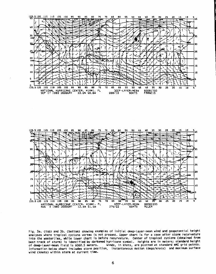
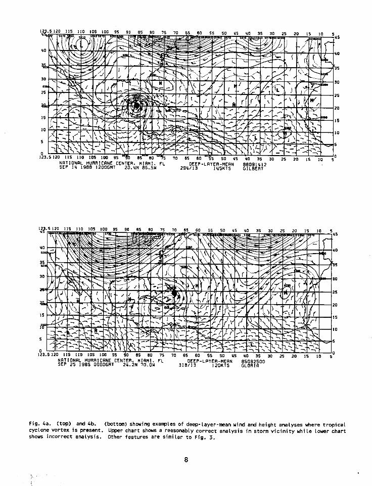
! t. Fig.4a. (top) aoo 4b. (bottcxn) showing exa~les of deep-layer-mean wioo 800 height analyses where tropicali l cyclone vortex is present. Upper chart shows a reasonably correct analysis in storm vicinity while lower chart

i shows incorrect analysis. Other features are similar to Fig. 3., II II .

'j..,I 8i I

I , .

The character of the initial analysis (and prognoses), examples ofwhich were depicted in Fig. 3 or Fig. 4 have a profound effect on theperformance of the NHC83 model. When the tropical cyclone vortex isnot present, as in Fig. 3, the wind and height fields near the storm 3typically give an excellent indication of the steering pattern. The 1'1 NHC83 model, being statistically tuned to this type analysis and

prognoses gives a forecast consistent with the synoptic pattern. Onthe other hand, situations as depicted in Fig. 4b, depending on thelocation of predictors, will mislead NHC83 and result in a degraded, tforecast. These conclusions are based on a review of all initial i ttropical cyclone analyses and resulting NHC83 errors from both devel- ~ (opmental and operational data over the period 1975-1988. i t

Until such time as the analysis and prognoses around the storm area ~becomes reasonably consistent, there is no short-term general statis-tical solution to the mis-analysis problem. However, to mitigate theproblem, more recent data could be used to develop the model. Also,a limit could be imposed such that predictors were selected no closerthan, say, 300 n mi (2 NHC83 or NHC90 grid points) from the storm ,center, to avoid interference from the vortex. .; j

! !

One possible long-term solution to the problem would be to develop a Iifilter for removing the tropical cyclone vortex from the analyses andprognoses. Although such methodology is conceptually appealing, thereare many problems. These are currently being addressed at NHC andelsewhere~ preliminary findings have not been used in developing NHC90. !

2.2.2 Bias in numerical forecasts -The Perfect-Prog method (seefootnote 3) used in developing NHC83 assumes that developmental and ;operational data have similar statistical characteristics. For the jyears 1983 through 1986, this assumption was valid. However, for the !1987 hurricane season, the 18-layer MRF (Medium Bange ~orecast) modelreplaced the older spectral model in the operational "Aviation-Run" :slot. The MRF has a cold bias which leads to an erosion of the Igeopotential heights (and an associated bias in the wind field) with ~. !time. This bias has been discussed by a number of authors including i!Saha and Alpert (1988), Epstein (1988), Schemm and Livesey (1988) and /.White (1988). I

The bias pattern across the Atlantic for the 1987 hurricane season was 'ishown in TM41, Fig. 21. At the 72 h projection, height biases (heights :forecast too low) of over 40 meters were noted through the sub-tropical !ridge line. Inasmuch as the standard deviation of the heights in that

Iarea is close to 20 meters, the heights are in error by as much as two' ;standard deviations. This is a potentially serious forecast problem:when storms are located in this area.

A bias correction methodology was introduced in NHC83 for the 1988 ,hurricane season (TM41, section 5.4). However, since that time, NMC 1 '

has made additional changes to the analysis/prognoses package which' ,appear to have altered the previous bias pattern of the MRF model and 'interfered with the correction methodology currently in place in the IiNHC83 model. I

!

9 ,~

~ !

85M 80H 15M 70H 65M 60H25N 25N

20N .20N Fig.5. Example of NHC83inconsistent track fore-

(=:> cast at 48 and 6Oh for..Hurricane Gilbert, Sept.

10, 120OUTC, 1988.15M 15N

, .'I '" ~\ ,~, ~-x:;,~ ~rJ ~ 10N I -~,.lOti iON

85M 80W 15M 70W 65!t 60W

Until the bias in the MRF model is removed or stabilizes, there is nocompletely satisfactory way of compensating for it. However, in thisrevision to the NHC83 model, particular care was used to select pre-dictors in pairs rather than as separate entities. Pairs of predictorsallow the model to sense gradients rather than rely solely on absolutevalues as was sometimes done in the NHC83 model. However, this use ofgradients may lead to a trade-off in predictive skill in some cases.

2.3 CORRECTABLE DEFICIENCIES

The final set of deficiencies are internal to the model and are'therefore largely correctable either by re-working the dependent dataor changing the set of predictors.

2.3.1 Inconsistencies in NHC83 Forecast Track -Figure 5 shows oneof the operational NHC83 track forecasts on Hurricane Gilbert, 1988.Here, it can be noted that the 48 hand 60 h forecast positions appearinconsistent with other segments of the track. This inconsistency hasbeen noted on virtually all NHC83 forecasts on storms embedded in theeasterlies.

The problem here can be traced to an inconsistent selection of predic-tors for the 48 and 60h projections. The location of these predictorsi are shown in Fig. 13 of TM41 under "across-track motion, perfect-prog ,

; mode, south-zone". The predictor located some 300 n mi to the south-i southwest at 48 h and at 60 h was excluded for the other forecasti periods. This exclusion leads directly to the track inconsistency

\noted in Fig. 5. In NHC90, a consistent set of predictors was main-tained for each forecast period and this deficiency appears to have.been corrected. I

2.3.2 Inconsistencies in NHC83 stratification Scheme -The NHC83 !model is stratified according to whether a storm is initially located!equatorward or poleward from 25°N. A different prediction method-ology is used in each of these two zones. The scheme assumes that astorm located in the south zone is moving with a component towards thewest. occasionally, this is not the case and relatively poor forecastsresult. A partial solution to this problem had been incorporated intothe NHC83 model for the 1988 season (see TM41, section 4.5). !

,, 10 J

- ~..c~~"~"~ ~

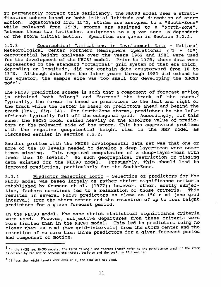
To permanently correct this deficiency, the NHC90 model uses a strati-fication scheme based on both initial latitude and direction of stormmotion. Equatorward from 15°N, storms are assigned to a "South-Zone"while poleward from 25°N, storms are assigned to a "North-Zone".Between these two latitudes, assignment to a given zone is dependenton the storm initial motion. Specifics are given in Section 3.2.2.2.3.3 Geoqraphical Limitations in Develo~ment Data -National ~Meteorological Center Northern Hemisphere operational ("3 + 45") rigeopotential height analyses over the years 1962 and 1981 were used ~for the development of the NHC83 model. Prior to 1975, these data were;represented on the standard "octagonal" grid system of that era which, ,jdepending on longitude, did not contain data equatorward from 10 to 113°N. Although data from the later years through 1981 did extend to ijthe equator, the sample size was too small for developing the NHC83 ~model. ~"

iThe NHC83 prediction scheme is such that a component of forecast motion'is obtained both "along" and "across" the track of the storm.STypically, the former is based on predictors to the left and right ofthe track while the latter is based on predictors ahead and behind thetrack (TM41, Fig. 14). For South-Zone storms, predictors to the left-of-track typically fell off the octagonal grid. Accordingly, for this izone, the NHC83 model ~elied heavily on the, absolute value of predic- 11tors on the poleward s1de of the storm. Th1S has aggravated problemsjwith the negative geopotential height bias in the MRF model asdiscussed earlier in section 2.2.2.Another problem with the NHC83 developmental data set was that one ormore of the 10 levels needed to develop a deep-layer-mean were some-times missing. This required computation of a deep-layer-mean withfewer than 10 levels.6 No such geographical restriction or missingdata existed for the NHC90 model. Presumably, this should lead toimproved prediction, particularly for the South-Zone. ;

i,2.3.4 Predictor Selection Loqic -Selection of predictors for the INHC83 model was based largely on rather strict significance criteriajestablished by Neumann et ale (1977): however, other, mostly subjec-tive, factors sometimes led to a relaxation of those criteria. This'resulted in several NHC83 predictors as close as 150 n mi (one grid "interval) from the storm center and the retention of up to four height ~predictors for a given forecast period. 1,'"

In the NHC90 model, the same strict statistical significance criteria /:were used. However, subjective departures from these criteria weremore limited than in the NHC83 model. This led to predictors being nocloser than 300 n mi (two grid-intervals) from the storm center and theretention of no more than three predictors for a given forecast period -and component of motion. j:

5 In the NHC83 and NHC90 models, the .te.~ "alon.g-." and "across-t.ra.ck" refer to .the persistence track of the storm Ias defined by the motion between the InItIal posItIon and the posItIon 12 h earlIer.6 If less than eight levels were available, the case was not used. ;t11 ,!

f

Although this "tightening" of standards is expected to improve uponthe performance of the model, this cannot be verified until therevised model has been used operationally for at least one hurricaneseason.

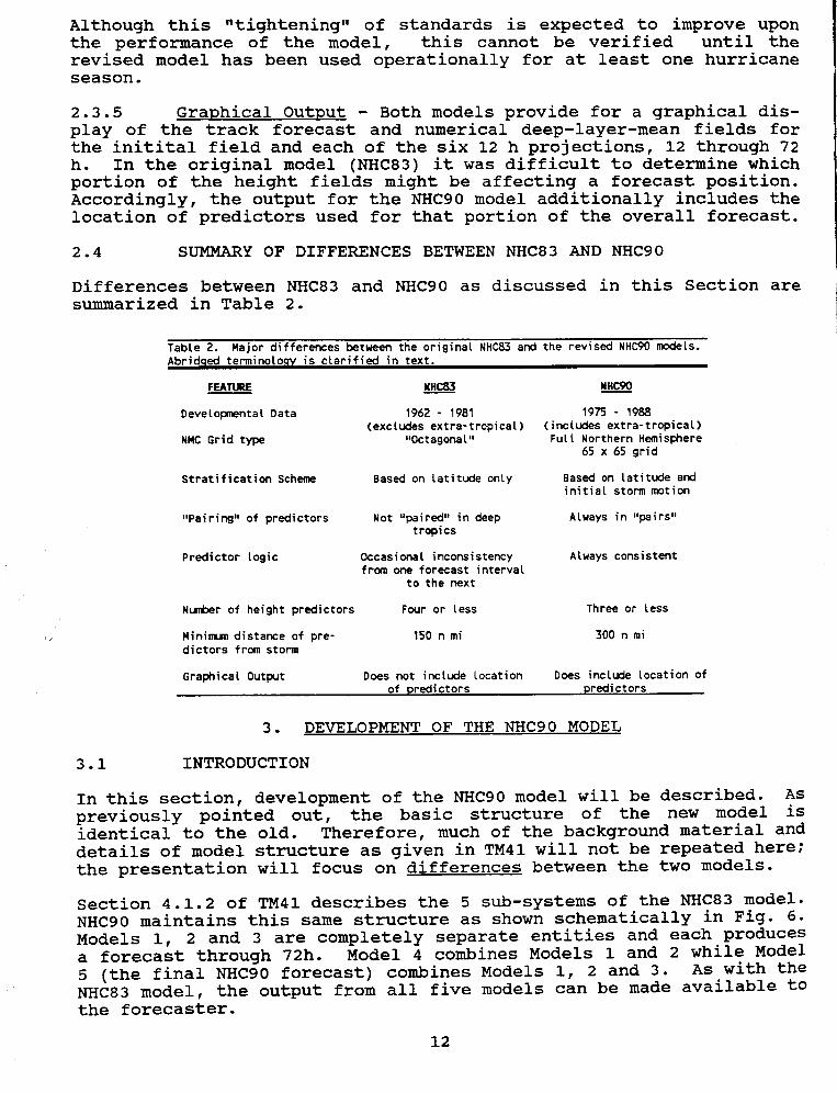
2.3.5 GraDhical OutDut -Both models provide for a graphical dis-play of the track forecast and numerical deep-layer-mean fields forthe in it ita I field and each of the six 12 h projections, 12 through 72h. In the original model (NHC83) it was difficult to determine whichportion of the height fields might be affecting a forecast position.Accordingly, the output for the NHC90 model additionally includes thelocation of predictors used for that portion of the overall forecast.

2.4 SUMMARY OF DIFFERENCES BETWEEN NHC83 AND NHC90

Differences between NHC83 and NHC90 as discussed in this Section aresummarized in Table 2.

Table 2. Major differences between the original NHC83 and the revised NHC90 nX>dels.AbridQed terminoloQv is clarified in text.

FEA~ ~ ~

Developmental Data 1962 -1981 1975 -1988(excludes extra-tropical) (includes extra-tropical)

NMC Grid type "Octagonal" Full Northern Hemisphere65 x 65 grid

Stratification Scheme Based on latitude only Based on latitude andinitial storm motion

ifi "Pairing" of predictors Not "paired" in deep Always in "pairs"

i .tropics

i Predictor logic Occasional inconsistency Always consistentl from one forecast intervalI 'cc..: to the next'I!; f'

hi Number of height predictors Four or less Three or less, I

...iMInImum dIstance of pre- 150 n mi 300 n mi fdictors from storm I

,Graphical OUtput Does not include location Does include location of i

of credictors credictors \

I 3. DEVELOPMENT OF THE NHC90 MODEL

i !1 3.1 INTRODUCTIONl:. In this section, development of the NHC90 model will be described. As

previously pointed out, the basic structure of the new model isidentical to the old. Therefore, much of the background material anddetails of model structure as given in TM41 will not be repeated here;the presentation will focus on differences between the two models.

section 4.1.2 of TM41 describes the 5 sub-systems of the NHC83 model.NHC90 maintains this same structure as shown schematically in Fig. 6.Models 1, 2 and 3 are completely separate entities and each produces

: a forecast through 72h. Model 4 combines Models 1 and 2 while Modeli 5 (the final NHC90 forecast) combines Models 1, 2 and 3. As with the

NHC83 model, the output from all five models can be made available to

f the forecaster.l,

! 12i,~ I

"L..~ """"..~"c.;.."",..

,-I

CLIMATOLOGY OBSERVED FORECASTAND GEOPOTENTIAL GEOPOTENTIAL -!

;

PERSISTENCE HEIGHTS HEIGHTS 1,Fig 6. Schematic of the five r

(MOOEL 1) (MOOEL 2) (MOOEL 3) c~ts (lOOdels) used by ;,I'

I I 1 1 the NHC83 and NHC90 lOOdels. ~ ,

! The term ~ refers to I t! ! ! ! Q.eep-!:.ayer-Mean. Model 2 is ~ .,L E ~ J referred to as "ANALYSIS" ~ I I

..MOOEL I. ..while Model 3 is referred to ij .:as the "PERFECT-PROG" lOOde. ~ IIi' , '.

; !:' i ,

NHC90 FORECAST ~ I:+- -~ ; ,

(MOOEL 5) , i.I : .~ '. ~

3.2 DEVELOPMENTAL DATA ~ II,

3.2.1 SamDle size -The developmental data set used by NHC90 !iincludes all Atlantic tropical cyclone cases having winds of at least ,.i34 knots (tropical storm intensity or greater). Over the 14-year [1 1period, 1975-1988, positions at 0000 and 1200 UTC were used. These ;,1 I

were paired with associated Northern hemisphere National Meteorological !Center operational gridded analyses through the 72h projection. In _

I I'accordance ,with ,perfect-progmethodology, analyses were substituted for'prognoses ln thlS developmental mode. 1

Although archived analyses were available prior to 1975, those analysesdid not contain data in the deep tropics and use of these early dataled to some problems with the NHC83 model (see section 2.3.3). Accord- ,ingly, pre-1975 data were not used for NHC90. The total sample sizeavailable for NHC90 development was 935 cases. This is somewhat lessthan the 1028 cases used in developing NHC83 but is still large enough! jto allow stratifying the data set into two zones, a North-Zone and a ~..

South-Zone, as was accomplished with the NHC83 model. ,I ,

In both models, storms which were below tropical storm strength, ei ther I':at the initial or verifying position, were excluded. However, in the i .!NHC90 model, tropical cyclones classified as extra-tropical were jretained whereas in NHC83 they had been excluded. There were two 1reasons for this difference: (1) exclusion of the extratropical cases ~ ~

in NHC90 would have critically reduced the sample size; (2) inC1USionl: I

of the extra-tropical cases increased, rather than decreased the .l

variance reduction on developmental data.

3.2.2 stratification -stratification of a data set into two or , Imore groups typically improves model performance in terms of real,skill. However, there is also an increase in artificial skill due to ,the reduction in sample size. consequently, additional stratifi- 11cation was avoided.

i!

)

13 ,\

t

j

, -.-, .I "",,"""-_.,,-"

f

I ,-.

One of the most logical stratifications separates storms embedded in: the easterlies (South-Zone storms) from those embedded in the wester-

lies (North-Zone storms). Statistically, this helps in normalizingthe data set, a desirable feature in regression analysis. In Fig. 2,for example, the distribution of the 72 h errors is distinctly bi-

i model and this results from combining errors from storms in both zonesr (Crutcher et al., 1982).t

Ii There ar~ a~so theoretic~l factors favoring a mo~ion stratification.; Storms w1th1n the easter11es tend to move to the r1ght (poleward) from

the steering flow while those within the westerlies tend toward the:. left (also poleward) from the basic flow (Brand et ale 1981); (Dong and

Neumann, 1986); (George and Gray, 1976).

For NHC83, a rather simple criteria --initial position poleward orequatorward from 25°N --was used to separate storms embedded in the

f easterlies from those in the westerlies. As pointed out in Section2.3.2, this was not entirely satisfactory; a somewhat more definitivesystem was used for NHC90:

(1) Storms initially located poleward from 25°N were assigned toa North-Zone.

: (2) Storms initially located equatorward from 15°N were assigned.,i.. to a South-Zone.,i 'f'i

1! (3) Storms initially located between the above specified lati-tudes were assigned to the South-Zone only if their motion was between180°, clockwise to 320°, inclusive. Otherwise, they were assigned tothe North-Zone.

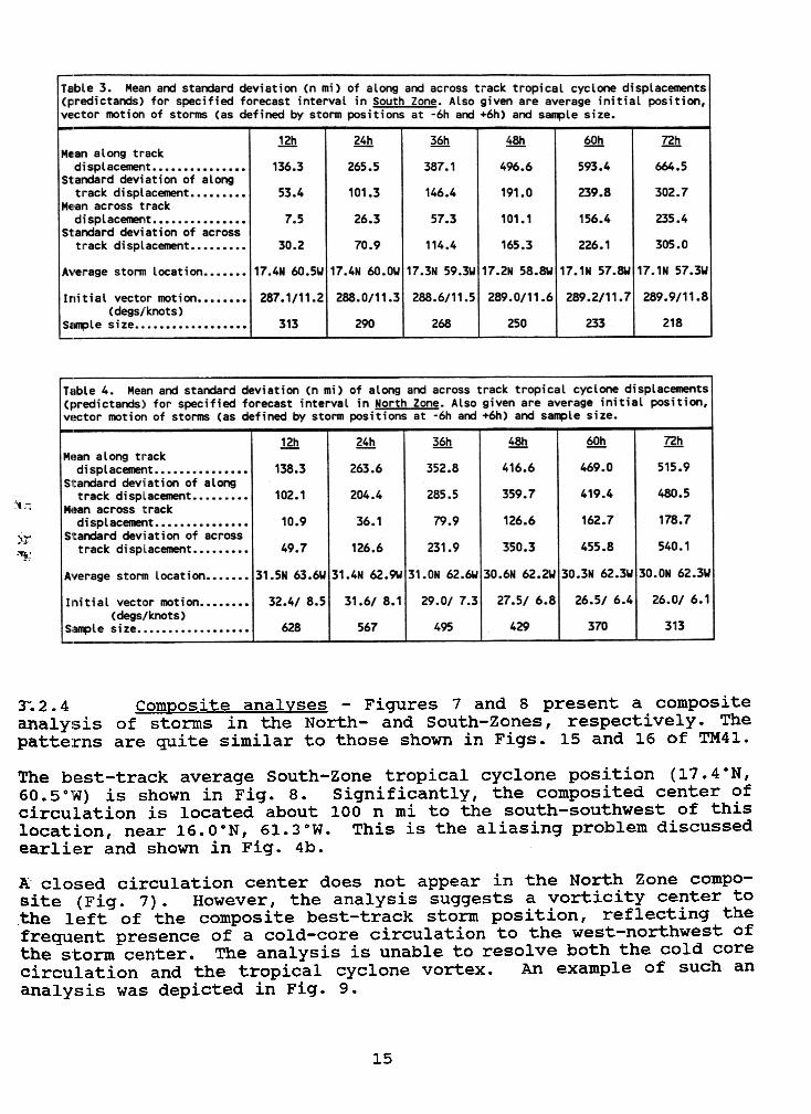
3.2.3 Sta~istical Attributes of Develoumental Data -The statis-tical properties of the two data sets obtained from the above definedstratification scheme are given in Tables 3 and 4. As described inTM41, the NHC83 model prediction scheme is based on alona-track andacross-track components (see footnote 4). This same orthogonal systemwas maintained in NHC90.

r['The above tables are identical in format to their counterparts --i Tables 3 and 4 --in TM41. As would be expected, there are some; differences in the statistical properties of the developmental data of'I

; the two models. In can be noted, for example, that the averageposition of South-Zone storms in NHC90 is near 17°N whereas in NHC83,this average is near 21°N. This rather substantial difference reflectsthe stratification scheme between the two models. South-Zone stormsbeing farther equatorward in NHC90 also leads to rather substantialdifferences in the vector motion for this zone between the two models; Iabout 303° for NHC83 and 287° for NHC90. '

,For North-Zone storms, differences between the data sets of the two: models are comparatively small. Indeed, most of the differences! between the two models, including performance on developmental data

(to be discussed in a later Section) are on South-Zone storms.,:

!;

14!

~

H

~~

",'".'J

~

3'.2.4 ComDosite analyses -Figures 7 and 8 present a compositeanaly~sis of storms in the North- and South-Zones, respectively. Thepatte:r-ns are quite similar to those shown in Figs. 15 and 16 of TM41.

1~

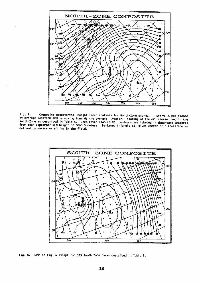
The best-track average South-Zone tropical cyclone position (17.4°N,60.5°1iV) is shown in Fig. 8. Significantly, the composited center ofcirculation is located about 100 n mi to the south-southwest of thislocation, near 16.00N, 61.3°W. This is the aliasing problem discussedearlLer and shown in Fig. 4b.

A' closed circulation center does not appear in the North Zone compo-site (Fig. 7). However, the analysis suggests a vorticity center to,the left of the composite best-track storm position, reflecting thefrequent presence of a cold-core circulation to the west-northwest ofthe s'torm center. The analysis is unable to resolve both the cold corecirculation and the tropical cyclone vortex. An example of such ananalysis was depicted in Fig. 9.

15

.

.,-,

NORTH-ZONE COMPOSITE I

i

55

i.,..1

/50

4

140

Fig. 7. Composite geopotential height field analysis for North-Zone stonms. Stonn is positionedat average location and is moving towards the average (vector) heading of the 628 storms used in theNorth-Zone as described in Table 4. Deep-Layer-Mean (DLM) contours are labeled in departure (meters)from mean September DLM height of 6060.5 meters. Darkened triangle (~) gives center of circulation asdefined by maxima or minima in the field.

SOUTH-ZONE COMPOSITE

10

5

Fig. 8. Same as Fig. 4 except for 313 South-Zone cases described in Table 3.

16

15

0

5

0

25 ;.,'1r'

20 H

i

15 '1

'110 \

~

0 .-123.5120 115 110 105 100 95 90 85 80 75 50 J

NATIONAL HURRICANE CENTER. MIAMI. FL DEEP-LATER-MEAN 87D9D912 jSEP 9 1987 12DDGMT 3S.7N 37.9W 037/17 3SKTS CINDT ~

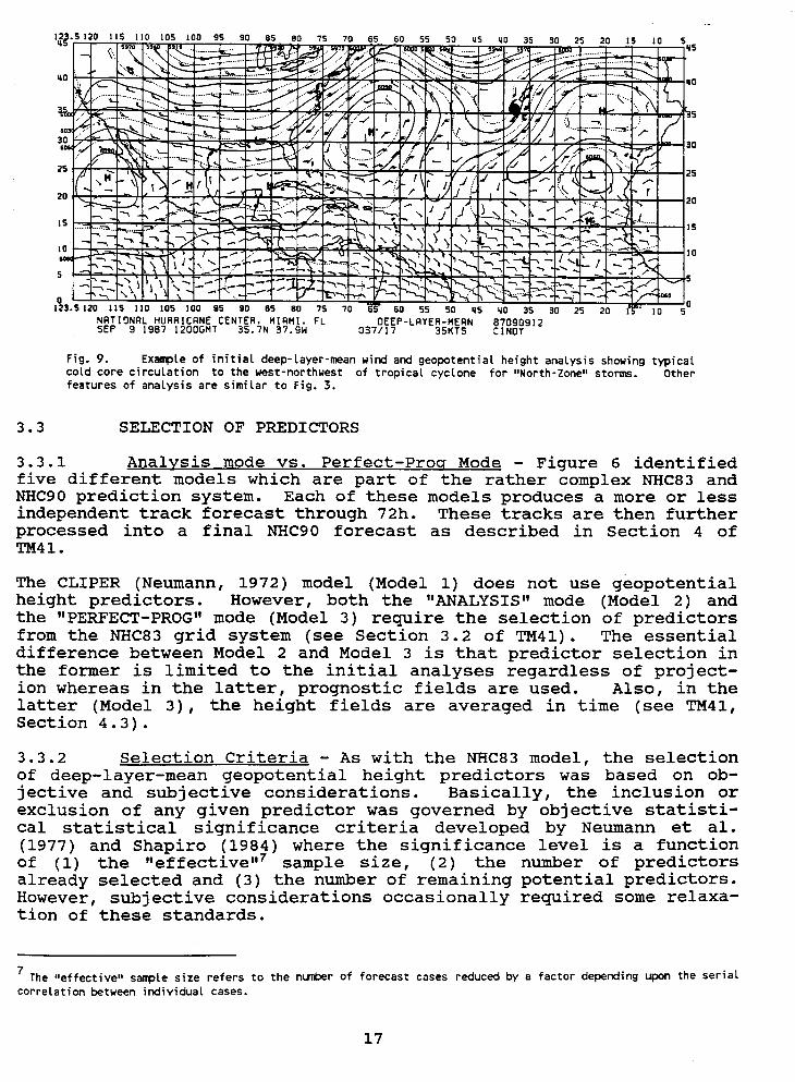
'iFig. 9. Example of initial deep-layer-mean wind and geopotential height analysis showing typical '4

cold core circulation to the west-northwest of tropical cyclone for "North-Zone" storms. Other ':features of analysis are similar to Fig. 3.

3.3 SELECTION OF PREDICTORS

3.3.1 Analysis mode vs. Perfect-Proa Mode -Figure 6 identified ifive different models which are part of the rather complex NHC83 and.NHC90 prediction system. Each of these models produces a more or less

Iindependent track forecast through 72h. These tracks are then further.processed into a final NHC90 forecast as described in section 4 ofTM41.

The CLIPER (Neumann, 1972) model (Modell) does not use geopotentialheight predictors. However, both the "ANALYSIS" mode (Model 2) andthe "PERFECT-PROG" mode (Model 3) require the selection of predictorsfrom the NHC83 grid system (see Section 3.2 of TM41). The essential 1difference between Model 2 and Model 3 is that predictor selection in ,I...the former is limited to the initial analyses regardless of project- .!ion whereas in the latter, prognostic fields are used. Also, in the;latter (Model 3), the height fields are averaged in time (see TM41, :.Sectl.on 4.3).

3.3.2 Selection criteria -As with the NHC83 model, the selection Iof deep-layer-mean geopotential height predictors was based on ob-jective and subjective considerations. Basically, the inclusion or :exclusion of any given predictor was governed by objective statisti- ~cal statistical significance criteria developed by Neumann et ale 1(1977) and Shapiro (1984) where the significance level is a function

!of (1) the "effective"7 sample size, (2) the number of predictorsalready selected and (3) the number of remaining potential predictors.However, subjective considerations occasionally required some relaxa-

ftion of these standards. j , ,

; The "effective" sample size refers to the number of forecast cases reduced by a factor depending upon the serial :

correlation between individual cases. ;.

t17 ,

i

~~

This relaxation was needed to force predictor selection in pairs(gradients). Pairing was considered mandatory to minimize the biasproblem noted in the NHC83 model. Also, it was required to avoid theproblem with NHC83 depicted in Fig. 5 where the forecast track containsunrealistic changes in motion from one forecast interval to another.

3.3.3 pairinq of Predictors -As with NHC83, selection of height!predictors in the NHC90 model utilized the paired predictor concept

described in Section 3.3.3 of TM41. The goal here is to insure thatthe two most heavily weighted predictors, which represent steering,are the best that can be selected. Considerable subjective inter-vention is required during this step of the predictor screeningprocess. This is because the screening program only recognizes andselects one predictor at a time and is not sufficiently astute torecognize potential gradients. Pairs of predictors are identified bytrial and error methodology where all possible pairs are tested as totheir net variance reduction as well as to their consistency in thephysical sense.

3.3.4 ExamDle of Predictor Selection. North Zone. Along track -Some examples of initial predictor selection (before application ofthe pairing concept) are shown and discussed in this section. Examplesare for the "Perfect-Prog" mode (Model 3).

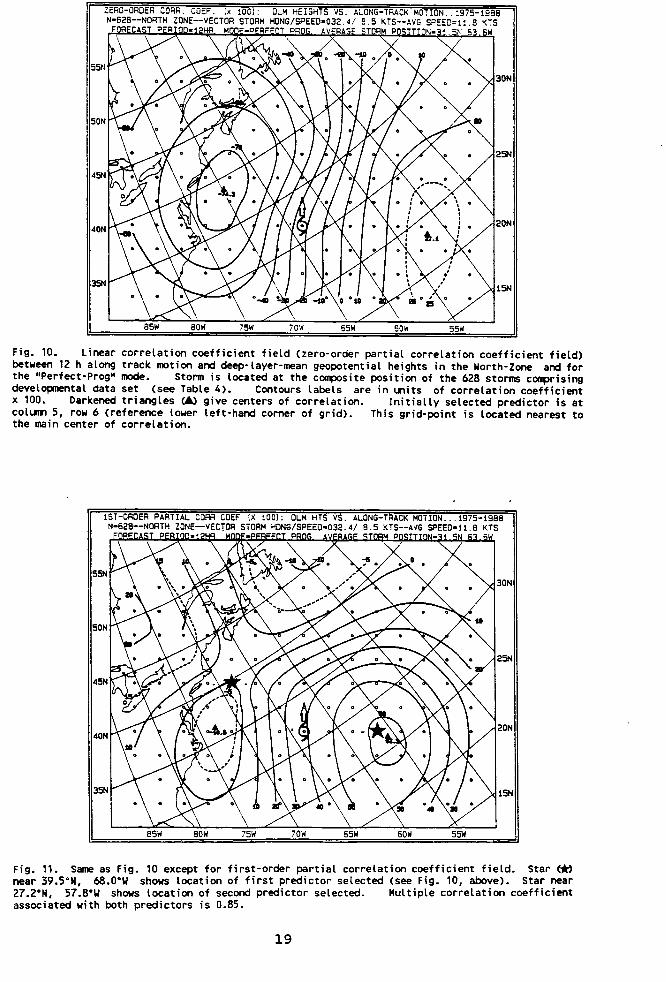
I' Figures 10 and 11, show, respectively, the zero-order and first-order

.partial correlation coefficient fields (Mills, 1955) for 12 h along-i track motion vs. height for the North-Zone. The counterpart of these

charts, for the NHC83 model, are given as Figs. 6 and 7 of TM41 and1 the marked similarity between fields reflects the strong statistical

stability in both models. It also reflects the fact that, except inthe near-equatorial regions, the two developmental data sets (1962 -1981 for NHC83, 1975 -1988 for NHC90) overlap for the years 1975 -1981.

To be noted in Fig. 11 is an area of residual negative correlation tothe left of the storm after selection of the initial predictor. This Ireflects the fact that the selected initial grid point (column 5, row.

1! 6)8 is not located at the exact center of correlation. conceptually,ij this situation could be corrected by an adjustment of the grid system.: However, it is believed that the use of predictors-in-pairs, discussed

in the previous Section (3.3.3), compensates for this small loss of Ipredictive potential. I

,

In that the two grid-point predictors chosen from these fields (asidentified on the figure legends) are actually working in harmony asa gradient but are selected as separate entities, they are not neces- Isarily the most efficient pair (see Section 3.3.3). It can be shown,for example, that predictors located somewhat closer to the stormcenter (column = 6, row = 5) and (column = 10, row = 4), net a signifi-cantly greater variance reduction. This latter pair is identified bytrial and error methodology, as discussed in section 3.3.3.

8 Reference point for grid (1,1) is the lower-left corner. Address of lower-right grid point is (15,1).

18!\: ,

ZERO-ORDER CDRR. COEF. Ix 100): Ot.M HEIGHTS VS ALONG-TRACK MOTION. .:975-1988N-628--NORTH ZONE-VECTOR STORM HONG/SPEED-032.4/ 8.5 KTS--AVG SPEED=1~.8 KTS

55~ON

.'

50

.; 5N;!

45

I_.ON

cf' 40

,,-

:;::- 35 5N ii

.i *'"

~;" ~ i"'"'

Fig. 10. linear correlation coefficient field (zero-order partial correlation coefficient field)between 12 h along track motion and deep-layer-mean geopotential heights in the North-Zone and forthe "Perfect-Prog" mode. Storm is located at the c~site position of the 628 storms c~rising

t developmental data set (see Table 4). Contours labels are in units of correlation coefficient.'~ x 100. Darkened triangles ~ give centers of correlation. Initially selected predictor is at

~ colllln 5, row 6 (reference lower left-hand corner of grid). This grid-point is located nearest to ; ,f the main center of correlation. i :

« ~..' I III

1ST-ORDER PARTIAL CORR COEF (X 100): DlM HTS VS. AlONG-TRACK MOTION...1975-1988I'

N-628--NDRTH ZONE-VECTOR STORM HDNG/SPEED-032.4/ 8.S KTS--AVG SPEEO-11.8 KTS~1~ P I

i

.IN 1 ': ,

,.. i

i50 j , !

5N .1

45 J !

, !

ON !40 ,

;~

35 5N t i, i

; f i,, ,

:

Fig. 11. Same as Fig. 10 except for firs~-order ~rtial correlation c~fficient field. Star ~Inear 39.5°N, 68.0oW shows location of fIrst predIctor selected (see FIg. 10, abo~e). Sta~ ~ear

27.2°N, 57.8°W shows location of second predictor selected. Multiple correlat10n coefflc1entassociated with both predictors is 0.85.

J19 :.,

f

tt

3.3.5 Examples of Predictor Selection. North Zone. Across Track -Figures 12 and 13 are similar to Figs. 10 and 11 except that theypertain to across-track motion and are for 72 h, rather than 12 h. Asdiscussed in TM41, section 4.3,72 h fields are actually average fieldsfor the seven time periods, 00, 12, 24, 36, 48, 60 and 72 h. Theaveraging is accomplished after grid-rotation (see footnote 5) andafter translation to the observed storm position at the appropriate -;,prO]ect10n. S1m1larly, the 12 h fields are the average of 00 hand 12h relative grids, etc.

Figures 12 and 13 are very similar in pattern to their counterparts,Figs. 8 and 9 in TM41. As with Figs. 10 and 11, this reflects unusualstability in the model. The two initially selected predictors, as .

identified in the figure legends, represent a large-scale gradientacross the storm and are indicative of imQlied rather than direct csteering. However, the predictors-in-pairs concept, discussed'earlier, leads to selection of a more efficient set, positioned closer jto the storm vortex and more indicative of direct steering. These;latter (and final) locations of geopotential height predictors are ~

depicted in Figs. 16 and 17.

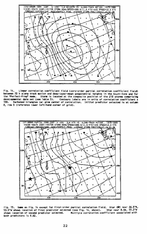
3.3.6 Example of Predictor Selection. South Zone. Alona Track -Afinal example of preliminary predictor selection (for the South-Zone)is given in Figs. 14 and 15. The counterpart of Fig. 14 in TM41 isFig. 10. Because of the absence of data equatorward from the storm(see section 2.2.3) in the NHC83 model, there is no counterpart of Fig. .15 in TM41. As was the case with the other two examples of predictor fselection, the overall pattern of the correlation field is very "Isimilar between the two models. 1

As shown in Fig. 14, most of the predictive information for South-Zone 1storms is to the right, rather than to the left of the storm, as was 1the case for North-Zone storms. This reflects the importance of the ~subtropical ridge line in controlling the motion of these storms. -1

After the selection of an initial predictor at (column = 8, row = 5),Fig. 15 shows a weak but statistically significant area of correla-tion to the left-rear (southwest) of the storm. In the interest ofmitigating the bias problem (see Section 2.2.2), a predictor from thisarea was included in the NHC90 model. This was considered anacceptable trade-off considering other risks associated with use ofpredictors in the deep tropics; specifically, low standard deviationsof the heights used as predictors, as well as uncertainties in theanalyses and numerical prognoses.

3.3.7 Final Selection of Predictors -Figures 10 through 15 showedexamples of preliminary predictor selection for the Perfect-Prog mode.Similar procedures are followed for the selection of Analysis modepredictors except that the current analysis is used for every forecastinterval.

After the application of predictor-pairing methodology, a furthersearch is made through second-order partial correlation fields forareas of additional predictive information. Typically, other t~anfor the two "steering" predictors (zero- and first-order part1al

20

Fig. 12. Linear correlation coefficient field (zero-order partial correlation coefficient field)between 72 h across track motion and deep-layer-mean geopotential heights in the North-Zone and for ;the Perfect-Prog mode. Storm is located at the composite position of the 313 storms comprising idevelopmental data set (see Table 4). Contours labels are in units of correlation coefficient x '100. Darkened triangles (.) give center of correlation. Initially selected predictor at column f

"10, row 9 (reference lower left-hand corner of grid). This grid point is located nearest to the 1main correlation center. j

:

Iij

!; ,

j

j:J:J J,

.Fig. 13. Same as Fig. 12 except for first-order partial correlation field. Star ~ near 38.S0N, I49.SoW shows location of first predictor selected (see Fig. 12, above). Star near 2S.1°N, 71.0oW

Ishows location of second predictor selected. Multiple correlation coefficient associated with bothpredictors is 0.92. i

21 :

~

f

".l

i'

t,

"

;'Ii'-

I:;

..,

Fig. 14. Linear correlation coefficient field (zero-order partial correlation coefficient field)between 72 h along track motion and deep-layer-mean geopotential heights in the South-Zone and forthe "Perfect-Prog" mode. Storm is located at the c~site position of the 218 storms c~isingdevelopmental data set (see Table 3). Contours labels are in units of correlation coefficient x100. Darkened triangles (6) give center of correlation. Initial predictor selected is at column8, row S (reference lower left-hand corner of grid).

1ST-ORDER PARTIAL CaRR COEF IX 100): OLM HTS VS. ALONG-TRACK MOTION.. .1975-1988N-218--S0UTH ZONE-VECTOR STORM HONG/SPEEDs289.9/11.B KTS-AVG SPEEO-12.3 KTS

P -7 M -P RF R AV P w

Fig. 1S. Same as Fig. 14 except for first-order partial correlation field. Star ~ near 26.S.H,S3.SoW shows location of first predictor selected (see Fig. 14, above). Star near 8.0N, 5S.2°Wshows location of second predictor selected. Multiple correlation coefficient associated withboth predictors is 0.82.

22

correlation fields}, additional significant predictors were not found.The exception was for along-track motion in the Perfect-Prog mode :where, for all projections, 12 through 72 h, an additional significant !height predictor was identified to the left-of-track. I

II"iIn all, t~ere ar7 eiCJ:ht sets of geopotential height predictors for each : If

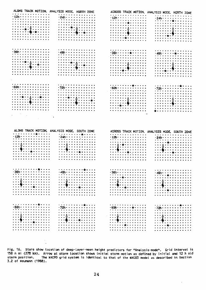
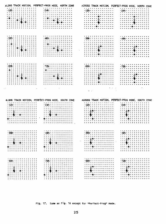
of the SlX prO]ectlons, 12 through 72 h. Four sets are for the ~,Analysis mode and another four sets are for the Perfect-Prog mode. I;specific locations of the predictors for these modes, respectively,are shown in Figs. 16 and 17.

4. MODEL PERFORMANCE ON DEVELOPMENT DATA i

4.1 REDUCTIONS OF VARIANCE ,,\r'

4.1.1 Review of Model stru~tur~ -As briefly pointed out in SectionI3.1 and as shown schematically in Fig. 6, the NHC83 and NHC90 are

developed from the output o,f thre~ ?ifferent models. T~ese have been I'referred to as Modell (Whlch utlllzes only those predlctors relatedto climatology and persistence), Model 2 (which utilizes onlypredictors derived from current deep-layer-mean height analysis) and [

IModel 3 (which utilizes only predictors derived from "forecast" ;jfields). Each of these models produces a forecast track through 72 h. ~

~I

The output from these three models, in the form of along- and across-track displacements, are then used as dependent data for the develop-ment of a final forecast (Model 5). In an operational mode, Model 4(which is a combination of Models 1 and 2) is used as a "first-guess" I

for positioning the grids in the numerical fields. Model 4 is not usedin the developmental mode. Additional details on this process are

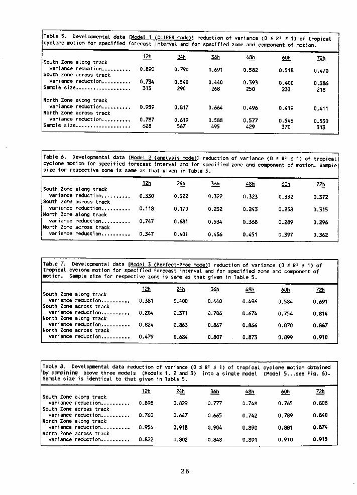
given in TM41.Reductions of variance which were obtained from Models 1, 2 and 3 aregiven in Tables 5, 6 and 7 while those from the combined Model 5 aregiven in Table 8. Table 5 was not included in TM41; however, thelatter three tables, for the NHC83 model, appear in TM41 as Tables 5, ,6 and 7. !

4.1.2 QgmQarison of vsr~an~e. Red~ct.i,o~~ -In comparing variancereductions, it should be noted that reduction of variance (R2) is given :by the relationship, ':

R2 = 1 -S 2 / s 2 (1)e y

where R is the multiple correlation coefficient, Si is the standarderror (standard deviation about the regression ine, surface orhyperplane) and S is the standard deviation about the mean of the

predictand. Thus~ for given values of Se' R2 (and R) are directly

proportional to Sy., ' . f ' d t ' S t

Because R2 is a relatlve quantlty, comparlson 0 varlance re uc lon,from different models is typically obscured by differences in stan-

Idard deviation of the predictands. In general, however, an examina-tion of these tables indicates that, for the analysis mode (Model 2), Ithe NHC83 model has somewhat higher variance reductions than does thenew model. However, for the Perfect-Prog mode (Model 3), the reverse!

23 :

:!

I"~. ._c. " C"C"...~~c..~

~

ALONG TRACK MOTION. ANAL YSIS MOO~ NORTH ZONE ACROSS TRACK MOTION. ANALYSIS MOO~ NORTH ZONE'12h .24h .12h"""..,.., '24h""'",.",

* *~ *.

~ ~ ~ *. * * * * .36h. 48h. 36h. *. 48h' *. *.

~ *. ~ ~ "".' . ~ * * * * * * .60h' ". .72h.'""...", .60h .72h..'...",...

"'.' '...'.. ,; *. .

~...*... *. . £"..'.. ~ ~ *. * * , ,

l' .A~~N.G. ~:K. :°.r~~~ .ANAL Y~:S. ~O.O~. ~~~ .Z~. ~~.O~: :~~C~ .M?~I~~.. ANAL ~S:: .M?~~ .S.O~. ~O~:

.12h.""' , .24h '12h .24h..".."..",; * :: :~::::::::::: :: :~::::::::::: :: :~:~::::::::: :: :~:::::::::::

* * * * * * .36h '48h .36h."' "" '48h' ""...

* * :::~::::::::::: :::~::::::::::: :::~::::::::::: :::~:::::::::::

; * * * .'.".."""'.* I, , , .

,'i * * * .60h. 72h. 60h. *. 72h. ...

~ ~ ~ ~ '" * ! ::::::: :~:::::: ::::::::::::::: ::::: :~:::::::: :::: :~:::::::::

Fig. 16. Stars show location of deep-layer-~an height predictors for "Analysis-mode". Grid interval is150 n mi (278 Km). Arrow at storm location shows initial storm motion as defined by initial and 12 holdstonn position. The NHC90 grid system is identical to that of the NHC83 model as described in section3.2 of Neunann (1988).

24

,

ALONG TRACK MOTIO~ PERFECT -PROG MOO~ NORTH ZONE ACROSS TRACK MOTIO~ PERFECT -PROG MOO~ NORTH ZONE

.1211"""""" .24h '12h'""""", '24h""::::::::'. :'.::: : :~.::::::: : :.::::.:::.:::: :::::: :*::::::: :::::: :*:::::::

*. *.~ ~ .~ * ,.* ..,... ., , * * """"""'" .36h' , 4Bh' 36h 4Bh' !i

,: :.:::::::::::: : :.:::::::::::: .:::::::::::::::::::::::::::::: ~~ ~ ~* ~* ~*. *. I* * ""'" """ .* * ,

I'60h"""""" .72h'""""", .60h'""""", .7211"""""" ~.* .* ,

:::: :.:~::::::: :::: :.:~::::::: :::::: :~~:::::: :::::: :~~:::::: :,.* ,.* , , ')

::::::::::::::: ::::::::::::::: :::::: :.::::::: :::::: :.::::::: i

ALONG TRACK MOTIO~ PERFECT-PROG MOO~ SOUTH ZONE ACROSS TRACK MOTION. PERFECT-PROG MOO~ SOUTH ZONE

'1211"""""" '24h"""""" '12h"""""" '24h""""""

:::~::::::::::: :::~::::::::::: :::~~:.::::::::: :::~~::::::::::...,. .* ...,. .* ..., ..., , * * * * .., ,

""""""" .36h' 4Bh' 36h' 4Bh' I

, :::~::::::::::: :::~::::::::::: :::~~:::::::::: :::~~::::::::::

...,. .* ...,. .* ..., ..., , """"""'" , .

* * * * .., 1

,... ;'60h ' .72h"""""" '60h"""""" '72h"""""" ~

,. , t, """"""'" ...~ ...~ ...~* ...~* .I ..',""""'" ..'.""""'" ..'.""""'" ..',""""'"

t ~~ ~ ~ ~ ~r~ ~ ~ ~ ~ ~ ~ ~ ~~ ~ ~ ~ ~r~ ~ ~ ~ ~ ~ ~ ~ ~ ~ ~ ~~~ ~ ~ ~ ~ ~ ~ ~ ~ ~ ~ ~ ~ ~~~ ~ ~ ~ ~ ~ ~ ~ ~ ~,;;~

Fig. 17. Same as Fig. 16 except for "Perfect-Prog" mode."

., 25~

" I

t " ,'.,~j i !"" ,I 1

! :rt ,I ' .!

:

iI

!i! ITable 5. Develo~ntal data [Model 1 (CLIPER mode)] reduction of variance (0 ~ R2 ~ 1) of ": cyclone motion for specified forecast interval and for specified zone and component of motion.

l I r?h ill ~ ~ QQ!!. Z?h I I: Ii ISouth.Zone along ~rack I I,

!! I var1ance reduct10n 0.890 0.790 0.691 0.582 0.518 0.470ISouth Zone across track I

; I variance reduction 0.734 0.540 0.440 0.393 0.400 0.386 I IISample size 313 290 268 250 233 218 I 1

~I I1 ~ North Zone along track j.

I variance reduction 0.939 0.817 0.664 0.496 0.419 0.411!? I North Zone across track !

I varia~e reduction 0.787 0.619 0.588 0.577 0.546 0.530Sample s1ze 628 567 495 429 370 313

; ~ !; .!;' I

; "I illit~

i .[,1 !cyclone motl0n for speclfled forecast lnterval and for speClfled zone and component of motlon. Sample I! , size for respective zone is same as that given in Table 5.

I r?h ill ~ ~ QQ!!. Z?h I:, ISouth.Zone along ~rack I J;: I varlance reductIon 0.330 0.322 0.322 0.323 0.332 0.372 I I'; South Zone across track'1 I variance reduction 0.118 0.170 0.232 0.243 0.258 0.315 I

INorth Zone along track II variance reduction 0.747 0.681 0.534 0.368 0.289 0.296

INorth Zone across trackI variance reduction 0.347 0.401 0.456 0.451 0.397 0.362 II I

,Table 7. Develo~ntal data [Model 3 (Perfect-ProQ mode)] reduction of variance (0 ~ R2 ~ 1) of itropical cyclone motion for specified forecast interval and for specified zone and component of

Imotion. Sample size for respective zone is same as that given in Table 5.

12h 24h 36h 48h 60h 72hSouth Zone along track Ivariance reduction 0.381 0.400 0.440 0.496 0.584 0.691

South Zone across trackvariance reduction 0.204 0.371 0.706 0.674 0.754 0.814

,! North Zone along trackI\ variance redJction 0.824 0.863 0.867 0.866 0.870 0.867

" North Zone across track

!'. variance reduction 0.479 0.684 0.807 0.873 0.899 0.910""! !;

Table 8. Develo~ntal data reduction of variance (0 ~ R2 ~ 1) of tropical cyclone motion obtained

by combining above three models (Models 1, 2 and 3) into a single model (Model 5...see Fig. 6).Sample size is identical to that given in Table 5.

r?h ill ~ ~ 2Qh Z?hSouth Zone along track

variance reduction 0.898 0.829 0.777 0.748 0.765 0.808South Zone across track

variance reduction 0.760 0.647 0.665 0.742 0.789 0.840North Zone along track

variance reduction 0.954 0.918 0.904 0.890 0.881 0.874North Zone across track 15

variance reduction 0.822 0.802 0.848 0.891 0.910 0.9

26i

t.l

:

~,i .:!

if

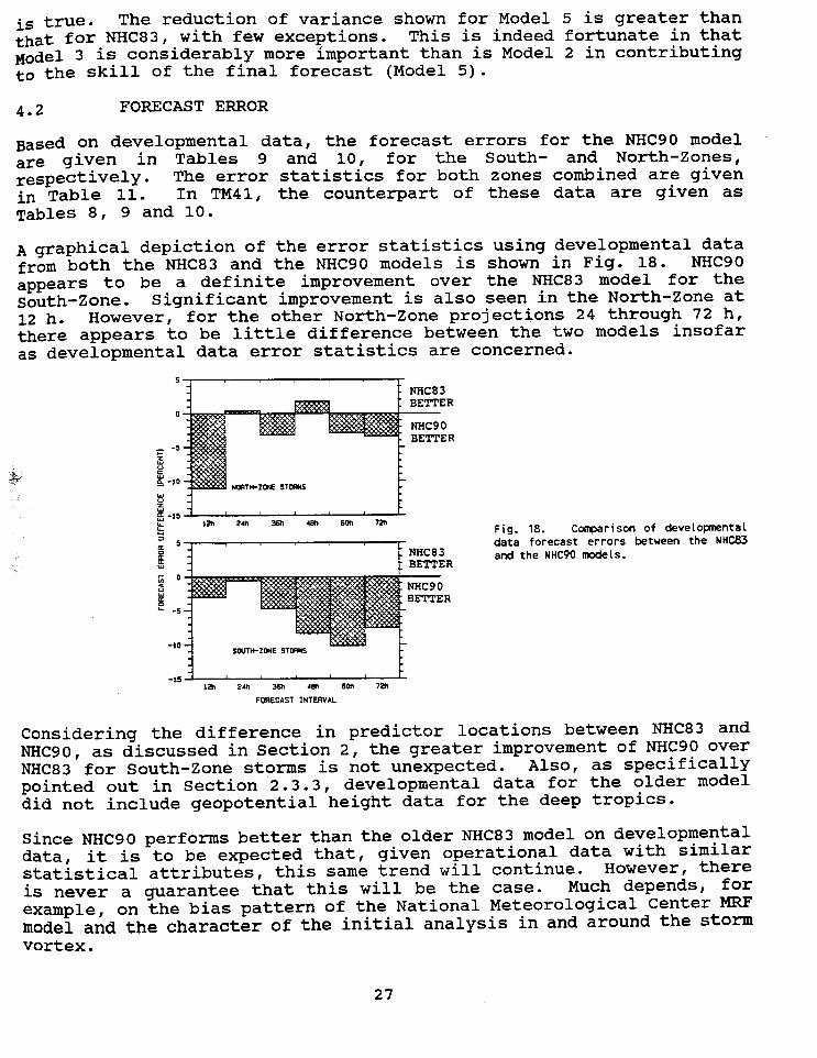
is true. The reduction of variance shown for Model 5 is greater thanthat for NHC83, with few exceptions. This is indeed fortunate in thatModel 3 is considerably more important than is Model 2 in contributingto the skill of the final forecast (Model 5).

4.2 FORECAST ERROR,}

Based on developmental data, the forecast errors for the NHC90 model I!are given in Tables 9 and 10, for the South- and North-Zones, Irespectively. The error statistics for both zones combined are given!in Table 11. In TM41, the counterpart of these data are given as ~!Tables 8, 9 and 10. I !

IIA graphical depiction of the error statistics using developmental data ~from both the NHC83 and the NHC90 models is shown in Fig. 18. NHC90 jJappears to be a definite improvement over the NHC83 model for the I t

south-Zone. Significant improvement is also seen in the North-Zone at I'12 h. However, for the other North-Zone projections 24 through 72 h, t

there appears to be little difference between the two models insofar' 1.as developmental data error statistics are concerned. [: !

5

R i: :0 ': i

'1 !..i

R I i--5 I;.w...

~; ~-IOw...

zwa: -15~ 1211 2'" 3611 4811 6011 7211~ Fig. 18. Comparison of developmental~ 5 data forecast errors between the NHC83~ and the NHC90 nX)dels.w R..0'"<...w~0

5

!-10 SMH-Z- ST~ 1

!,-15 .

12112411 3611 .81160117211 ii'

FORECAST INTERVAL .

Considering the difference in predictor locations between NHC83 and !NHC90, as discussed in section 2, the greater improvement of NHC90 over

"NHC83 for South-Zone storms is not unexpected. Also, as specifically C ipointed out in section 2.3.3, developmental data for the older model ldid not include geopotential height data for the deep tropics. ISince NHC90 performs better than the older NHC83 model on developmental t.

data, it is to be expected that, given operational data with similar.statistical attributes, this same trend will continue. However, thereis never a guarantee that this will be the case. Much depends, forexample, on the bias pattern of the National Meteorological Center MRFmodel and the character of the initial analysis in and around the storm

vortex.,

27 t

,i

..~._""".,,"'-,_.. c- ..'-",-,,-~.~

'"t

I Table 9. Developmental (dependent data) forecast errors (n mi) on South Zone storms for Model 1 ~

(CLIPER), Model 2 (analysis mode) and Model 3 (Perfect-Prog mode). Also given are forecast errors Ifrom Model 4 (CLIPER & Analysis) and Model 5 (CLIPER, Analysis and Perfect-Prog).

Errors from: .1£!!. ~ ~ ~ 2Q.b. Zfh

MODEL 1 (CLIPER) 19.8 57.4 104.6 160.1 218.3 289.4MODEL 2 (ANALYSIS) 44.3 90.7 136.0 184.4 239.1 302.0MODEL 3 (PERFECT-PROG) 42.8 83.6 116.7 144.1 167.3 187.5MODEL 4 (Models 1 and 2

coobined) 19.2 54.4 98.4 148.3 197.9 255.1MODEL 5 (Models 1, 2 and 3

coobined) , 18.7 50.0 82.7 111.5 137.2 158.5

Percentage improvement ofModel 5 over Model 1 5.6 12.9 20.9 30.4 37.2 45.2

Sample size 313 290 268 250 233 218

Table 10. Developmental (dependent data) forecast errors (n mi) for North Zone storms for Model 1(CLIPER), Model 2 (analysis mode) and Model 3 (Perfect-Prog mode). Also given are forecasterrors from Model 4 (CLIPER & Analysis) and Model 5 (CLIPER, Analysis and Perfect-Pros).

\Errors from: .1£!!. ~ ~ ~ 2Q.b. Zfh



coobined) 24.8 68.7 108.9 144.7 175.1 205.5


Sample size 628 567 495 429 370 313

Table 11. Developmental (dependent data) forecast errors (n mi) on North and South Zones coobinedfor Model 1 (CLIPER), Model 2 (analysis mode) and Model 3 (Perfect-prog mode). Also given are fore-cast errors from Model 4 (CLIPER & Analysis) and Model 5 (CLIPER, Analysis and Perfect-Pros).

Errors from: .1£!!. ~ ~ ~ 2Q.b. Zfh



coobined) 22.8 62.4 99.7 132.5 160.5 186.2


Sample size 941 857 763 679 603 531

28

I

FORECRST rIA IS 36 VAL I 0 AT 90091110G I---

C) SsGSW 60W SSW SOW 4SW 40W 3SWm S~f

0 " I..-0 ..I,

I-.J :]a: c.so ON c; .

I,~

CXJ IiI; I .. "c ~.. },~- C\/ i

4S SN i'1

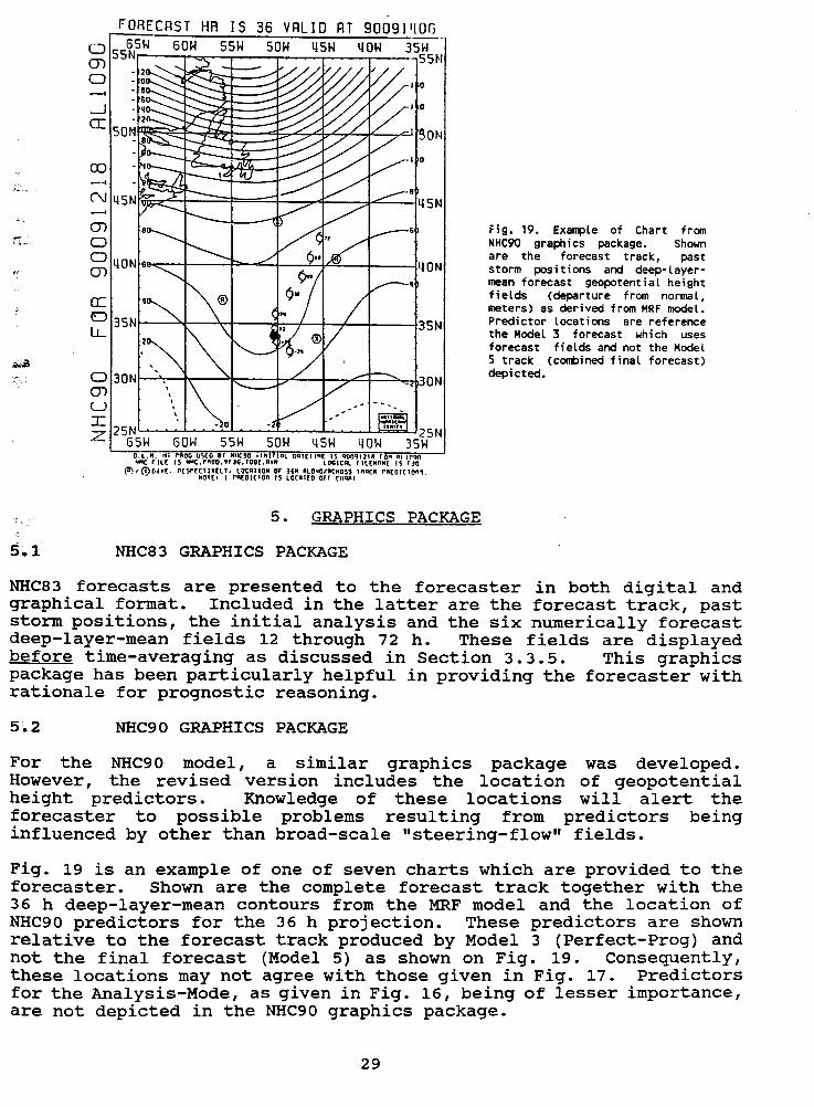
!m Fig. 19. Example of Chart from ~ ~

;y. 0 NHC90 grap,ics pacKage. Shown R i040 are the forecast tracK, past 1

" m ON storm positions and deep-layer- 'I I.,. mean forecast geopotential height

fields (departure from normal, "; a: meters) as derived from MRF model. I ' .."

-0 3S 3SN Predictor locations are reference ;t

LL the Model 3 forecast which uses !"forecast fields and not the Model

~', 5 t~acK (combined final forecast) !~ 0 30N ON depICted. ~

m ~,U ;

i ,J: }- i11-2SN SN ;! )~ GSW GOW SSW SOH 4SH 40W 3SH ~ ;j

O.l.". H' '"'01; "S(O B' "HC90 -'"IIIOl 001[1'"( IS _0'2'" ron 0""00 : 4""c rilE IS ""C."00.,r36.1001.A'" lOGICAL rllE"n"[ IS rJG t t(O)'@r.I'E. "rs"rCII'(lT. lOCAIIO" OF 36" AlONG/AC"OSS ,nAC. "'(o'r'cn, , ,

"CI(o I ,"AECICIon IS lCCAI[C orr [HO.' ,;,0

5. GRAPHICS PACKAGE

5.1 NHC83 GRAPHICS PACKAGE..

NHC83 forecasts are presented to the forecaster in both digital andgraphical format. Included in the latter are the forecast track, paststorm positions, the initial analysis and the six numerically forecastdeep-layer-mean fields 12 through 72 h. These fields are displayedbefore time-averaging as discussed in Section 3.3.5. This graphics ipackage has been particularly helpful in providing the forecaster with 1"rationale for prognostic reasoning. '

5.2 NHC90 GRAPHICS PACKAGE

For the NHC90 model, a similar graphics package was developed.However, the revised version includes the location of geopotentialheight predictors. Knowledge of these locations will alert the ~forecaster to possible problems resulting from predictors being ~influenced by other than broad-scale "steering-flow" fields. {:! Fig. 19 is an example of one of seven charts which are provided to the I

forecaster. Shown are the complete forecast track together wi~h theI36 h deep-layer-mean contours from the MRF model and the locat10n of

NHC90 predictors for the 36 h projection. These predictors are shown J;relative to the forecast track produced by Model 3 (Perfect-Prog) and, I,not the final forecast (Model 5) as shown on Fig. 19. consequentlY, ! ;

these locations may not agree with those given in Fig. 17. predictors!for the Analysis-Mode, as given in Fig. 16, being of lesser importance,are not depicted in the NHC90 graphics package. i

f29 1

t .~. ,. ,.,,".

- ~,y; .-:

I6. POTENTIAL FOR ADDITIONAL IMPROVEMENT TO NHC90

r6.1 GRID ROTATION

6.1.1. The NHC83/~C~0 System -Tropical cyclone motion is a vector tquant1ty. Most stat1st1cal models treat both orthogonal components ofmotion as separate entities and then combine them to produce a vector Iquantity. Typically, the orthogonal coordinate system is based on Iearth-oriented zonal and meridional components of motion which are notindependent in the statistical sense. As discussed by Shapiro andNeumann (1984), this practice leads to a slow-speed bias and increasedforecast error. The authors suggested a coordinate system based onalong- and across-track components where, by definition, the across-track component is initially near-zero and the forecast problem isinitially univariate, rather than bivariate.

NHC83 and NHC90 are structured according to the Shapiro/Neumann system.In view of the fact that NHC83 performs very well for the short-rangeprojections (see section 1.2.1), the rotation system is apparentlyI very sound. However, for the extended forecasts (beyond 36 h), thereis some question as to the efficiency of the Shapiro/ Neumann system,as was pointed out by the authors.

6.1.2 Proposed NHC90 Grid Rotation Svstem -The loss in efficiencyof the Shapiro/Neumann grid rotation system for extended projections

, is due to gradual increases in the across-track component of stormmotion throughout the 72 h forecast cycle. This is particularlynoticeable for North-Zone storms where most of the storm recurvatureinto the westerlies takes place. As noted in Table 4, for example,the mean/standard deviation of across-track storm motion in the NorthZone increases from 11/50 n mi at 12 h to 179/540 n mi at 72 h.

To compensate for this temporal loss in efficiency of the Shapiro/Neumann grid-rotation system, pike (1987b) suggests a grid rotationbased on the axis of zero-correlation in a bivariate normal fit to theobserved components of storm motion. This angle e, (Hope and Neumann,1970) is given by,

e = ~ TAN-1 [2rXYSxSy/ (SX2 -Sy2)] (2)

where Sx and Sy' are the standard deviations of zonal and meridionalmotion, respectively, and rXY is the linear correlation coefficientbetween components. Using a period of record, 1946 through 1988, theserotation angles and related data needed by Eg. (2) are given in Table12 for both the North- and South-Zone. Note that this period of recordis (intentionally) different than that used in developing the NHC90model (1975-1988).

Two examples of the bivariate fit to the storm motion data are shown;in Figs. 20 and 21. In that the limiting chi-square value at the 0.05 ;

probability level is 23.68 (see Crutcher et al., 1982), and in that thechi-squares computed from the data exceed this value, the bivariatefits are not particularly good. It appears that the major of the twomarginal normal distributions are skewed to the right (towards higher

30

,

I 1-

displacements). A bivariate log-normal distribution or a datatransformation might have been appropriate here. However, this factorshould not significantly affect the rotation of the major axis, whichis of interest here.

The Pike rotation system is much easier to apply than is the Shapiro/Neumann system. In the latter, grid rotation is different for eachindividual case. However, in the Pike system, grid rotation is fixedfor a given zone and projection.

~In association with the development of NHC90, a preliminary test of the ;1Pike rotation system was conducted using the rotation angles given in 'jTable 12. For the South-Zone, there was little difference between'developmental data forecast errors for the Shapiro/Neumann system and .Jthe Pike system. ~ ;

'For the North-Zone, the test indicated that the current Shapiro/ I t:Neumann sys.tem ga~.e better results at the, 12 ,and 24 h pr~jections. ~ fThere was ll.ttle dl.fference at the 36 h pro]ectl.on but the Pl.ke systemwas clearly superior at 48 and 72 h. These results are similar to thefindings of Pike.

This test suggests that the Pike rotation system should be incorporated;into the NHC90 for the extended projections in the North-Zone and it I'is considered likely that this modification to NHC90 will be, .accomplished. The current model, however, as reported on herel.n,utilizes the Shapiro/Neumann system exclusively.

ITable 12. Statistical properties of proposed grid-rotation system. Rotation :1a le e is in the mathematical sense. Period of record is 1946 -1988. : ,

Projection 12 h 24 h 36 h 48 h 60 h 72 h \' !

North-Zone Sx (n mi) 109.6 200.6 278.5 347.7 411.5 467.7 c;North-Zone S (n mi) 82.4 152.2 210.8 259.0 300.5 335.6North-Zone y (degs) 25.5 26.0 26.0 25.5 25.0 24.6North-Zone rxy (0~r~1) 0.36 0.36 0.36 0.37 0.38 0.39 .

South-Zone S (n mi) 56.8 109.9 164.1 222.6 289.5 354.8 ISouth-Zone SX (n mi) 44.1 86.9 129.7 172.5 215.2 255.2 ~South-Zone y (degs) -20.2 -13.4 -3.3 9.3 16.7 19.1 ,South-Zone r fO~r~1' -0.22 -0.12 -0.03 0.09 0.20 0.27xy,v_,-" v.-- , 4

J

~

i1.

i,

31 t

.,

i

I

!J't

~

~ t

~':

, "

'.

';;-1"

!::;.-",I Ruv .o-:oB7 NO~ --

"U --416.2 N.Mi. ~

V- 215.0 N.Mi.

~ '

t...., ..'.'. :. ...::. IFig. 20. Zonal and meridional c~nents ;,;

° ° ,of 48 h tropical cyclone moti~n, 1946 -f;

1988, for the "South-Zone" as fltted to a'!,..bivariate normal distribution. Origin of i

: -: elliptical axes indicates c~sited ini-

.~~ .tial storm position (17.7"N, 61.4°IJ).

~ ..Linear correlation between c~nents,

..average component motion, rotation angle,,. .-value of chi-square and sa~le size are as ~

specified. ~,

~'THETA. 9.3 DEGS DISTANCE SCAlE IN N.M!. ,

CHISG .44.8 1".-I._III-~M_I._III"""'~"""'"IIII;;;o; !.,N .1892 0 200 ADO 600 BOO l'

~:

i.

Ruv -0.368

U. 139.2 N.Mi. ..

V- 297.3 N.Mi. ..,

'. .i,. .:. ~

.; v00. .0

..". : 0.. '

.0:..0::. Fig. 21. Similar to Fig. 20 except for.: ° ..0. "North-Zone". C~sited storm position."0 is at 28.6N, 66.3\J.

THETA. 25.5 DEGS ..DISTANCE SCAlE IN NMI.

CHISG .39.4 11"11I.~II.'MIIIMIII'I'I'MI"MIIIIIII"IIIIMIMlI'..1I1N .2885 0 200 ADO 600 .BOO

.i:

\;1

, ..'ft

I 1

I!

32

I

",;

,.'..cc

:...,:

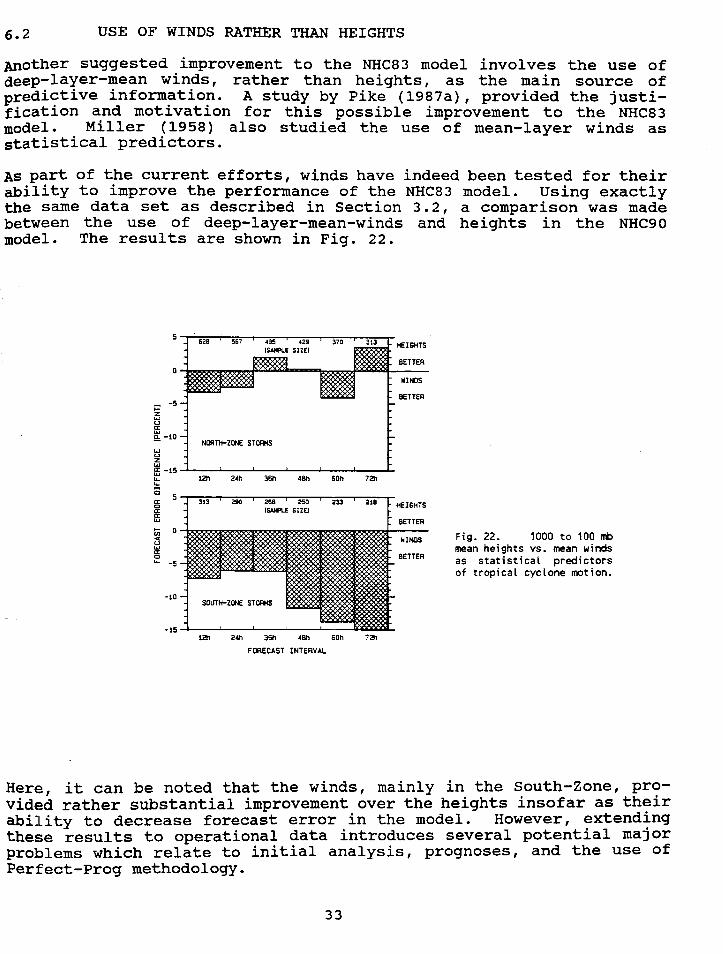
16.2 USE OF WINDS RATHER THAN HEIGHTS~,jAnother suggested improvement to the NHC83 model involves the use of'I deep-layer-mean winds, rather than heights, as the main source of '~predictive information. A study by Pike (1987a), provided the justi- i;I fication ~nd motivation for this, possible improvement to th7 NHC83 a.,: model. MJ.ller (1958) also studJ.ed the use of mean-layer wJ.nds as I

~"statistical predictors. i

I' As p~rt of t.he current efforts, winds have indeed been tested for their i~ abilJ.ty to J.mprove the performance of the NHC83 model. Using exactly; the same data set as described in sec~ion 3.2, a ?ompar~son was made -

between the use of deep-layer-mean-wJ.nds and heJ.ghts J.n the NHC90 ,

i 1 model. The results are shown in Fig. 22. I

J .Iiff(!! 5 ~67 HEIGHTS ;

~ ''I:, BETTER t!~ O Jir!J IfI~S !.

'~cC BETTERCo --s.-

z~.,.. w-~~; w

0i' Q. -1~ -N~TH-ZONE STORMS

l i_Is~~ ~ 1211 24h 36h 4Bh SOh 7211" "-~ 0;

5~ 290 268 250 233 218

;.;I: ~ ISAIPLf SIZEI':;;" ffi

.-0~ Fig. 22. 1000 to 100 mb~ mean heights vs. mean winds~ -5 as statistical predictors ;

of tropical cyclone motion.;;:'"

c -10SOUTIt-ZOHE STORMS

-151211 24h 36h 48n SOh 7211

FORECAST INTERVAL

,~

~

IHere, it can be noted that the winds, mainly in the South-Zone, pro-vided rather substantial improvement over the heights insofar as th7ir IabiJLity to decrease forecast error in the model. However, extendJ.ng .]" these results to operational data introduces several potential major

problems which relate to initial analysis, prognoses, and the use ofPerfect-Prog methodology.

331

1; ,

A review of Figs. 10 through 15 shows that, in the case of geo-potential heights, the centers of correlation and partial correlationare located at rather substantial distances from the storm center.Thus, analysis differences near the storm center, as illustrated inFigs. 3 and 4, are relatively unimportant insofar as the effect onthese distant predictors. However, for deep-layer-mean winds, as yetunpublished NHC studies have shown that the centers of correlationbetween storm motion and along/across track wind components are verynear the storm center. Accordingly, any mis-analysis near the stormcenter or changes in analysis methodology or numerical prognoses willhave a profound effect on the value of the statistical predictor andon the final forecast from the statistical model.

This is a difficult problem to address and further discussion on theuse of winds in an NHC83-type model is beyond the scope of the pre-sent study. Figure 22 indicates that winds do have the potential toimprove on the performance of the NHC83 and NHC90 models. Whetherthese results can be extended to operational data is not known at thistime.

7.0 LIST OF REFERENCES

Brand, S.C., C.A. Buenafe and H.D. Hamilton, 1981: Comparison oftropical cyclone motion and environmental steering. Mon. Wea. Rev.,1.09, 908-909.

Crutcher, H.L., C.J. Neumann and J.M. Pelissier, 1982: Tropicalcyclone forecast errors and the multimodal bivariate normaldistribution. Journ. ADDI. Meteor., 21., 978-987.

Dong, K. and C.J. Neumann, 1986: The relationship between tropicalcyclone motion and environmental geostrophic flows. Mon. Wea. Rev.,1.1.4, 115-122.

Elsberry, R.L., W.M. Frank, G.J. Holland, J.D. Jarrell and R.L.I Southern, 1987: A global view of tropical cyclones. Re~ort of WMOi International WorkshoD on TroDical Cvclones, Bangkok, Thailand, 1985,

Office of Naval Research, 185 pp.

Epstein, E.S., 1988: How systematic are systematic errors? PreDrints,8th Conf. Numerical Weather Prediction, Amer. Meteor. Soc., 460-465.

George, J.E and W.M. Gray, 1976: Tropical cyclone motion andsurrounding parameter relationships. Journ. ADDI. Meteor., 1.5,1252-1264.

Hope, J.R. and C.J. Neumann, 1970: An operational technique forrelating th"e movement of existing tropical cyclones to past tracks.Mon. Wea. Rev., 98, 925-933.

McBride J.L. and G.J. Holland, 1987: Tropical-cyclone forecasting:A world~ide summary of techniques and verification statistics. ~ll.Amer. Met. Soc., 68, 1230-1238.

Miller, B.l., 1958: The use of mean layer winds as a hurricanesteering mechanism. NHRP ReDort No. 18, U.S. Department of Commerce,Washington, DC, 24 pp.

34

I!

~Mills, F.C., 1955: statistical methods. Holt, Rinehart and Winston,New York, NY, 625 pp.

Neumann, C.J., 1972: An alternate to the HURRAN tropical cycloneforecasting system. NOAA Technical Memorandum NWS SR-62, National .,oceanic and Atmospheric Administration, u.s. Department of Commerce, !'Washington, DC, 32 pp. ~ !

, i

Neumann, C:J., 1988: The National Hurricane Center NHC83 model. I ,iHQM Technlcal Memorandum NWS NHC 41, National Hurricane Center, I ..coral Gables, FL, 44 pp. .I

Neumann, C.J. and M.B. Lawrence, 1975: An operational experiment ! ,in the statistical-dynamical prediction of tropical cyclone motion. 'I" I

Mon. Wea. Rev. , 103, 665-673. ..=--- !" '

INeumann, C.J., M.B. Lawrence and E.L. Caso, 1977: Monte Carlosignificance testing as applied to statistical tropical cyclone [.prediction models. Journ. A!2!2l. Met., 16, 1165-1174. ' f

Neumann, C.J. and J.M. Pelissier, 1981a: Models for the prediction I! ';

of tropical cyclone motion over the North Atlantic: An operational;evaluation. Mon. Wea. Rev., 109, 522-538. ,i

NNeumann, C.J. and J.M. Pelissier, 1981b: An analysis of Atlantic htropical cyclone forecast errors, 1970-1979. Mon. Wea. Rev., 109,1248-1266.

Pike, A.C., 1987a: A comparison of wind components and geopotentialheights as statistical predictors of tropical cyclone motion.Extended Abstracts. 17th Conference on Hurricanes and TropicalMeteoroloqy, Amer. Meteor. Soc., 101-103.

Pike, A.C., 1987b: statistical prediction of track and intensity forEastern North Pacific tropical cyclones. Pre!2rints. loth Conferenceon Probabilitv and statistics in AtmosDheric Science, Amer. Meteor.Soc., J40-J41. t.

JSaha, S. and J. Alpert, 1988: systematic errors in NMC medium range 0

forecasts and their correction. Preprints. 8th Conference onNumerical Weather Prediction, Amer. Meteor. Soc., 472-477. .Schemm, J.E. and R.E. Livesey, 1988: Statistical corrections to theNMC medium range 700mb height forecasts. Pre2rints. 8th Conference on .Numerical Weather Prediction, Amer. Meteor. Soc., 478-483. ' f

IShapiro, L.J., 1984: Sampling errors in statistical models of .

tropical cyclone motion: A comparison of predictor screening and EOF ~

techniques. Mon. Wea. Rev., 11.2, 1378-1388. ., I!, '

Shapiro, L.J. and C.J. Neumann, 1984: On the orientation of grid j

dystems for the statistical prediction of tropical cyclone motion. '

IMon. Wea. Rev., 11.2, 188-199. I

White, G.H., 1988: systematic performance of NMC medium range ! "forecasts, 1985-1988. PreDrints. 8th Conference on Numerical Weather'. 'Prediction, Amer. Meteor. Soc., 466-471. I I

i .35 ' .

j

.i

c- ~.,.,.",""~~."

(. a revised national hurricane center€¦ · a revised national hurricane center nhc83 model...

Documents