an adaptive spectrally weighted structure tensor applied to tensor anisotropic nonlinear diffusion...
TRANSCRIPT

A N A D A P T I V E S P E C T R A L LY W E I G H T E D S T R U C T U R ET E N S O R A P P L I E D T O T E N S O R A N I S O T R O P I C N O N L I N E A R
D I F F U S I O N F O R H Y P E R S P E C T R A L I M A G E S
By
Maider J. Marin Quintero
A dissertation thesis submitted in partial fulfillment of the requirements for the degree of
DOCTOR OF PHILOSOPHYin
COMPUTING AND INFORMATION SCIENCE AND ENGINEERING
University of Puerto RicoMAYAGUEZ CAMPUS
June 2012
Approved by:
____________________________________ ____________________Shawn Hunt, PhD.Member, Graduate Committee Date
____________________________________ ____________________Vidya Manian, PhD.Member, Graduate Committee Date
____________________________________ ____________________Wilson Rivera, PhD.Member, Graduate Committee Date
____________________________________ ____________________Miguel Velez-Reyes, PhD.President, Graduate Committee Date
____________________________________ ____________________Nestor Rodriguez, PhD.Program Coordinator Date
____________________________________ ____________________Francisco Maldonado, PhD.Graduate School Representative Date

To my two Daniel with all my love.....

A C K N O W L E D G M E N T S
It is with immense gratitude that I acknowledge the support and help of Dr. Miguel
Veléz-Reyes. This dissertation would not have been possible without his dedication
and guidance through all my doctorate years working with him. I would like to
thank him for all the opportunities he put in front of me, for his friendship and
help in other aspects of my life. I also thank to Isnardo Arenas and professor Paul
Castillo for useful comments during the implementation process of this thesis. To
Julio Duarte-Carvajalino from the University of Minnesota for his comments in the
papers. Special thanks to my husband Daniel McGee for all his love and support.
For listening when I was confused and for proofreading this thesis and all papers
I had submitted during the course of this work.
Furthermore, I would like to thank to the Laboratory for Applied Remote Sensing
and Image Processing (LARSIP) staff in particular Maribel and Evelyn for all their
support, friendliness and for making my life easier. To all my friends that at some
point life put us together in LARSIP. In particular, I want to express my gratitude
to Santiago Velasco for his friendship and advice that guided me towards Image
Processing. I am also grateful to Maria C. Torres, Leidy Dorado, Samuel Rosario,
Victor Asencio, Fanny Nina, Andrea Santos, Miguel Goenaga and their families for
their friendship and support during all this years.
Thanks to the Mathematical Science Department for providing the funds for my
first two years of my doctorate and the Electrical and Computer Engineering De-
partment for providing the academic environment that has allowed me to grow as
both a professional and person. To the staff and director of the Computing and In-
iii

formation Sciences and Engineering Doctorate program for their friendliness and
understanding.
I wish to thank my parents Faride y Rafael for all their love and for the many
times they left everything in Colombia to come and support us during high stress
times. To my twin sister Deiry for the spiritual and moral support that you provide
me during all this time in the distance and my siblings Gelmy , Rafael and Mileidy
for always being there for me.
This work was supported by U.S. Department of Homeland Security under Award
Number 2008-ST-061-ML0002 and partial support also was provided under DHS
Award Number 2008-ST-061-ED0001. This work used facilities of the Bernard M.
Gordon Center of Subsurface Sensing and Imaging sponsored by the NSF ERC
program under award EEC-9986821. My last year was supported by NASA un-
der Award Number NNX10AM80H. The views and conclusions contained in this
document are those of the authors and should not be interpreted as necessarily rep-
resenting the official policies, either expressed or implied of the U.S. Department
of Homeland Security or the National Science Foundation or NASA.
iv

Abstract of Dissertation Presented to the Graduate School of theUniversity of Puerto Rico in Partial Fulfillment of the Requirements
for the Degree of Doctor of Philosophy.
A N A D A P T I V E S P E C T R A L LY W E I G H T E DS T R U C T U R E T E N S O R A P P L I E D T O T E N S O R
A N I S O T R O P I C N O N L I N E A R D I F F U S I O N F O RH Y P E R S P E C T R A L I M A G E S
ByMaider Judith Marin Quintero
2012
Chair: Miguel Veléz-Reyes,Ph.D Major Program: Computing and Information Science and Engineering.
A B S T R A C T
The structure tensor for vector valued images is most often defined as the average of
the scalar structure tensors in each band. The problem with this definition is the as-
sumption that all bands provide the same amount of edge information giving them
the same weights. As a result non-edge pixels can be reinforced and edges can be
weakened resulting in a poor performance by processes that depend on the struc-
ture tensor. Iterative processes, in particular, are vulnerable to this phenomenon.
In this work, a structure tensor for Hyperspectral Images (HSI) is proposed. The
initial matrix field is calculated using a weighted smoothed gradient. The weights
are based on the Heat Operator. This definition is motivated by the fact that in
HSI, neighboring spectral bands are highly correlated, as are the bands of its gradi-
ent. To use the heat operator, the smoothed gradient is modeled as the initial heat
distribution on a compact manifold M. A Tensor Anisotropic Nonlinear Diffusion
(TAND) method using the spectrally weighted structure tensor is proposed to do
two kind of processing: Image regularization known as Edge Enhancing Diffusion
(EED) and structure enhancement known as Coherence Enhancing Diffusion (CED).
Diffusion tensor and a stopping criteria were also developed in this work. Compar-
isons between methods show that the structure tensor with weights based on the
v

heat operator better discriminates edges that need to be persistent during the iter-
ative process with EED and produces more complete edges with CED. Remotely
sensed and biological HSI are used in the experiments.
vi
Resumen de la Disertación Presentada a la Escuela Graduada de laUniversidad de Puerto Rico en cumplimiento parcial of de los requisitos
para el grado de Doctor en Filosofía.
U N T E N S O R D E E S T R U C T U R A A D A P T I V OE S P E C T R A L M E N T E Y S U U S O E N D I F U S I O N
A N I S O T R O P I C A N O L I N E A R U S A N D O U NT E N S O R PA R A I M A G E N E S H I P E R E S P E C T R A L E S
PorMaider Judith Marin Quintero
2012
Concejero: Miguel Veléz-Reyes,Programa doctoral: Ciencias e Ingeniería de la Información y la Computación
R E S U M E N
El tensor de estructura para imágenes vectoriales es comúnmente definido como
el promedio de los tensores de estructura que ha sido previamente calculado para
cada banda de la imagen. El problema con esta definición es que ella asume que
todas las bandas proveen la misma cantidad de información de los bordes. Por
lo tanto le da el mismo peso a cada una de las bandas. Como resultado, pixe-
les que no son bordes son reforzados y los bordes pueden ser debilitados. Esto
hace que otros procesos que dependan del tensor de estructura den resultados
mediocres. Los procesos iterativos son los más vulnerables a este fenómeno. En
este trabajo se propone un tensor de estructura para imágenes HiperEspectrales
(IHE). El campo matricial inicial es calculado usando un gradiente suavizado pon-
derado. Los pesos son basados en el operador de calor. Esta definición es motivada
por una propiedad de las IHE y de su gradiente. Esta es: las bandas espectrales
que están cercanas son altamente correlacionadas. Para poder hacer uso del op-
erador del calor, el gradiente suavizado es modelado como la distribucion inicial
de calor en una variedad compacta denotada por M. Este tensor de estructura
será aplicado a la Difusión Anisotrópica No Lineal basada en Tensores (DANT)
vii

para hacer Difusión que Preserva Bordes (DPB) y Difusión que Realza Coherencia
(DRC). Comparación entre los métodos muestran que el tensor de estructura pon-
derado con pesos basados en el operador de calor discrimina mejor los bordes con
DPB y produce bordes mas completos con DRC. Estos métodos han sido aplicados
a IHE sensadas remotamente como tambien imágenes biológicas adquiridas con
microscopios hiperespectrales.
viii

C O N T E N T S
Abstract v
Resumen vii
List of Figures xiv
List of Tables xviii
List of Algorithms xix
1 background 1
1.1 Introduction . . . . . . . . . . . . . . . . . . . . . . . . . . . . . . . . . . 1
1.2 Hyperspectral Remote Sensing . . . . . . . . . . . . . . . . . . . . . . . 4
1.3 Problem Statement . . . . . . . . . . . . . . . . . . . . . . . . . . . . . . 12
1.4 Technical approach . . . . . . . . . . . . . . . . . . . . . . . . . . . . . . 13
1.5 Thesis Contributions . . . . . . . . . . . . . . . . . . . . . . . . . . . . . 16
1.6 Thesis Overview . . . . . . . . . . . . . . . . . . . . . . . . . . . . . . . . 17
2 literature review and definitions 19
2.1 Mathematical Notation . . . . . . . . . . . . . . . . . . . . . . . . . . . . 19
2.1.1 Definition of Images . . . . . . . . . . . . . . . . . . . . . . . . . 19
2.1.2 Convolution . . . . . . . . . . . . . . . . . . . . . . . . . . . . . . 21
2.1.3 Image Derivatives . . . . . . . . . . . . . . . . . . . . . . . . . . . 22
2.1.4 Some basic kernels . . . . . . . . . . . . . . . . . . . . . . . . . . 23
2.1.4.1 The mean Kernel . . . . . . . . . . . . . . . . . . . . . . 23
2.1.4.2 The Median Filter . . . . . . . . . . . . . . . . . . . . . 23
2.1.4.3 The Gaussian Kernel. . . . . . . . . . . . . . . . . . . . 24
2.1.4.4 Derivative of a Gaussian kernel . . . . . . . . . . . . . 24
2.1.4.5 The smoothed gradient. . . . . . . . . . . . . . . . . . . 26
ix

contents x
2.2 Definition of Tensor . . . . . . . . . . . . . . . . . . . . . . . . . . . . . . 26
2.2.1 Some Geometrical interpretations . . . . . . . . . . . . . . . . . 28
2.2.1.1 Tensor as ellipsoids . . . . . . . . . . . . . . . . . . . . 29
2.2.1.2 Tensor as a sum of weighted elementary orthogonal
tensors . . . . . . . . . . . . . . . . . . . . . . . . . . . . 29
2.2.1.3 Tensor as encoder of the local structure-Case 2-D and
3-D . . . . . . . . . . . . . . . . . . . . . . . . . . . . . 29
2.2.2 Classification of local neighborhoods . . . . . . . . . . . . . . . 33
2.2.2.1 Classification of local neighborhoods: 2-D Case . . . . 33
2.2.2.2 Classification of local neighborhoods: 3-D Case . . . . 34
2.3 Structure Tensor . . . . . . . . . . . . . . . . . . . . . . . . . . . . . . . 35
2.3.1 Directions vs. orientation . . . . . . . . . . . . . . . . . . . . . . 35
2.3.2 Estimation of the Local Structure Tensor . . . . . . . . . . . . . 36
2.3.3 Structure Tensor: The development of Gradient Based methods 36
2.3.3.1 Optimization Problem . . . . . . . . . . . . . . . . . . 36
2.3.3.2 Structure tensor as a covariance matrix . . . . . . . . . 39
2.3.3.3 Using Differential Geometry . . . . . . . . . . . . . . . 40
2.3.4 Scalar structure tensor . . . . . . . . . . . . . . . . . . . . . . . . 41
2.3.5 Vector-Valued Structure Tensor . . . . . . . . . . . . . . . . . . . 43
2.4 Image Processing using Geometrical PDEs . . . . . . . . . . . . . . . . 44
2.4.1 Physical background of diffusion . . . . . . . . . . . . . . . . . . 45
2.5 Divergence-based Diffusion . . . . . . . . . . . . . . . . . . . . . . . . . 48
2.5.1 Linear diffusion . . . . . . . . . . . . . . . . . . . . . . . . . . . . 49
2.5.2 Perona and Malik Isotropic nonlinear diffusion . . . . . . . . . 49
2.5.3 Tensor Anisotropic nonlinear diffusion . . . . . . . . . . . . . . 51
2.5.3.1 Anisotropic extension of the isotropic model based
on scalar diffusivity . . . . . . . . . . . . . . . . . . . . 52

contents xi
2.5.3.2 Coherence-Enhancing Diffusion . . . . . . . . . . . . . 52
2.5.3.3 Edge Preserving Diffusion . . . . . . . . . . . . . . . . 54
2.5.3.4 Difference between EED and CED . . . . . . . . . . . . 56
2.6 Finite difference schemes in images . . . . . . . . . . . . . . . . . . . . 57
3 the spectrally weighted structure tensor 60
3.1 Structure Tensor . . . . . . . . . . . . . . . . . . . . . . . . . . . . . . . . 60
3.1.1 Di Zenzo Structure Tensor . . . . . . . . . . . . . . . . . . . . . . 62
3.1.2 Classical structure tensor . . . . . . . . . . . . . . . . . . . . . . 63
3.1.3 Methods to Enhance the Local Orientation . . . . . . . . . . . . 64
3.2 The Spectrally weighted structure tensor . . . . . . . . . . . . . . . . . 66
3.2.1 Weights Based on the Median. . . . . . . . . . . . . . . . . . . . 66
3.3 Spectrally Weighted Structure Tensor Based on the Heat Operator . . 68
3.3.1 Motivation . . . . . . . . . . . . . . . . . . . . . . . . . . . . . . . 68
3.3.2 The Heat Operator . . . . . . . . . . . . . . . . . . . . . . . . . . 70
3.3.3 Weights Based on the Heat Operator . . . . . . . . . . . . . . . 71
3.3.4 Parameters used for the Structure Tensor. . . . . . . . . . . . . 75
3.4 Implementation Details . . . . . . . . . . . . . . . . . . . . . . . . . . . 77
3.5 Concluding Remarks . . . . . . . . . . . . . . . . . . . . . . . . . . . . . 80
4 tensor anisotropic nonlinear diffusion 81
4.1 Introduction . . . . . . . . . . . . . . . . . . . . . . . . . . . . . . . . . . 81
4.2 Eigenvalues of the proposed diffusion tensors . . . . . . . . . . . . . . 82
4.2.1 EED diffusion tensor . . . . . . . . . . . . . . . . . . . . . . . . . 83
4.2.2 CED Diffusion tensor . . . . . . . . . . . . . . . . . . . . . . . . 85
4.3 TAND as an Approximation to Local Diffusion . . . . . . . . . . . . . 88
4.4 Discretization of the divergence-based diffusion equation using a
tensor . . . . . . . . . . . . . . . . . . . . . . . . . . . . . . . . . . . . . 92
4.5 Solver and Preconditioner used . . . . . . . . . . . . . . . . . . . . . . 97

contents xii
4.6 TAND Algorithm . . . . . . . . . . . . . . . . . . . . . . . . . . . . . . . 98
4.7 Concluding remarks . . . . . . . . . . . . . . . . . . . . . . . . . . . . . 98
5 experimental results 102
5.1 Data . . . . . . . . . . . . . . . . . . . . . . . . . . . . . . . . . . . . . . 103
5.1.1 Data for EED . . . . . . . . . . . . . . . . . . . . . . . . . . . . . 103
5.1.2 Data for CED . . . . . . . . . . . . . . . . . . . . . . . . . . . . . 106
5.2 Parameter Selection . . . . . . . . . . . . . . . . . . . . . . . . . . . . . . 107
5.3 About the weights . . . . . . . . . . . . . . . . . . . . . . . . . . . . . . 109
5.4 Nonlinear diffusion vs. Tensor Anisotropic Diffusion . . . . . . . . . . 114
5.5 Comparison of the structure tensors using TAND . . . . . . . . . . . . 116
5.5.1 TAND for Edge Enhancing Diffusion. . . . . . . . . . . . . . . . 116
5.5.1.1 Experiments with A.P. Hill Image . . . . . . . . . . . . 116
5.5.1.2 Experiments with Indian Pines image . . . . . . . . . 116
5.5.1.3 Experiments with Forest Radiance 1 Image . . . . . . 121
5.5.1.4 Experiment with Cuprite Image . . . . . . . . . . . . . 123
5.5.2 TAND for Coherence Enhancing Diffusion. . . . . . . . . . . . . 123
5.5.2.1 Thyroid Cells Image. . . . . . . . . . . . . . . . . . . . 123
5.6 Comparison between the spectrally adapted and Weickert’s spatial
TAND. . . . . . . . . . . . . . . . . . . . . . . . . . . . . . . . . . . . . . 130
5.6.1 TAND for Edge Enhancing Diffusion . . . . . . . . . . . . . . . 130
5.6.2 TAND for Coherence Enhancing Diffusion . . . . . . . . . . . . 132
5.7 Concluding Remarks . . . . . . . . . . . . . . . . . . . . . . . . . . . . . 136
6 on publicly available remote sensing imagery 138
6.1 Concluding Remarks . . . . . . . . . . . . . . . . . . . . . . . . . . . . . 141
7 conclusions and future work 143
7.1 Conclusions . . . . . . . . . . . . . . . . . . . . . . . . . . . . . . . . . . 143
7.2 Future work . . . . . . . . . . . . . . . . . . . . . . . . . . . . . . . . . . 145
contents xiii
Appendix 147
a selected topics 148
a.1 Some definitions from Linear Algebra and Numerical Analysis . . . . 148
a.1.1 Rank of a Matrix . . . . . . . . . . . . . . . . . . . . . . . . . . . 148
a.1.2 Sparse and dense Matrices . . . . . . . . . . . . . . . . . . . . . . 148
a.1.3 Projection Methods to solve large linear systems . . . . . . . . . 149
a.1.3.1 BiCG . . . . . . . . . . . . . . . . . . . . . . . . . . . . . 151
a.1.3.2 BiCGStab . . . . . . . . . . . . . . . . . . . . . . . . . . 153
a.1.3.3 GMRES . . . . . . . . . . . . . . . . . . . . . . . . . . . 153
b a preconditioner for solving the finite difference discretiza-
tion of pdes applied to images 155
b.1 Linear systems and Preconditioners used to solve them . . . . . . . . . 155
b.1.1 Properties of the Linear System arising from TAND. . . . . . . 157
b.2 Peric preconditioner . . . . . . . . . . . . . . . . . . . . . . . . . . . . . 159
b.3 Experimental Results . . . . . . . . . . . . . . . . . . . . . . . . . . . . . 163
bibliography 165

L I S T O F F I G U R E S
Figure 1.2.1 Remote sensing acquisition and spectral sampling. . . . . . . . 5
Figure 1.2.2 Hyperspectral remote sensing Acquisition. . . . . . . . . . . . . 7
Figure 1.2.3 Image regularization, treated as the evolution of a surface. . . . 10
Figure 1.2.4 Structure Enhancement. . . . . . . . . . . . . . . . . . . . . . . . 11
Figure 1.4.1 Structure tensor flow chart . . . . . . . . . . . . . . . . . . . . . 14
Figure 1.4.2 TAND Flow chart . . . . . . . . . . . . . . . . . . . . . . . . . . . 16
Figure 2.1.1 Convolution. . . . . . . . . . . . . . . . . . . . . . . . . . . . . . . 21
Figure 2.1.2 Gaussian distribution Gσ and its discrete approximation. . . . 25
Figure 2.1.3 Derivatives of the Gaussian kernel in x and y−direction. . . . . 26
Figure 2.2.1 Ellipsoidal representation of a 3D tensor. . . . . . . . . . . . . . 28
Figure 2.2.2 Basic local structures of a tensor using tensor glyphs, 2-D case 30
Figure 2.2.3 Basic local structures of a tensor using tensor glyphs, 3-D case. 32
Figure 2.3.1 Smoothed Gradient vs. Structure Tensor. . . . . . . . . . . . . . 41
Figure 2.4.1 Scale-space produced by CED in a thyroid tissue. . . . . . . . . 47
Figure 2.5.1 Comparison between EED and CED. . . . . . . . . . . . . . . . . 55
Figure 2.6.1 Spatial grid of the 3 × 3 neighborhood of a pixel P. . . . . . . . 56
Figure 2.6.2 Rotational invariant property. . . . . . . . . . . . . . . . . . . . . 58
Figure 2.6.3 Pixels involved in the the finite difference schemes. . . . . . . . 59
Figure 3.3.1 Comparison of bands of a HSI with the bands of its gradient
component Ix. . . . . . . . . . . . . . . . . . . . . . . . . . . . . . 69
Figure 3.3.2 Weighting effect in pixels on heterogeneous and homogeneous
regions of Indian Pines. . . . . . . . . . . . . . . . . . . . . . . . 73
Figure 3.3.3 Integration scale on CED. . . . . . . . . . . . . . . . . . . . . . . 76
xiv
List of Figures xv
Figure 3.4.1 Flow chart describing the proposed Structure Tensor. . . . . . 79
Figure 4.2.1 Comparison of the classical structure tensor using κ2 = 1 and
κ2 defined as in (4.2.2). . . . . . . . . . . . . . . . . . . . . . . . 84
Figure 4.2.2 κ2 using (4.2.3). . . . . . . . . . . . . . . . . . . . . . . . . . . . . 86
Figure 4.2.3 Comparing κ2 using (4.2.3) and using (4.2.4). . . . . . . . . . . . 87
Figure 4.2.4 Proposed diffusion tensor for CED vs. ψ. . . . . . . . . . . . . . 88
Figure 4.4.1 Classical and rotational invariant difference schemes grids. . . 93
Figure 4.6.1 Flow chart of the TAND algorithm . . . . . . . . . . . . . . . . 99
Figure 5.1.1 HSI used for EED and its classification maps. . . . . . . . . . . 104
Figure 5.1.2 Cuprite Image and its ground reference map. . . . . . . . . . . 105
Figure 5.1.3 Original Images used for CED. . . . . . . . . . . . . . . . . . . . 107
Figure 5.2.1 κ1’s Entropy vs. TAND iterations . . . . . . . . . . . . . . . . . . 110
Figure 5.2.2 Relative entropy of κ1. . . . . . . . . . . . . . . . . . . . . . . . . 111
Figure 5.2.3 Images produced with relative entropy of κ1as the stopping
criteria. . . . . . . . . . . . . . . . . . . . . . . . . . . . . . . . . . 112
Figure 5.3.1 Varying s in (3.3.2) with TAND’s iterations n. . . . . . . . . . . 113
Figure 5.4.1 Nonlinear diffusion vs. tensor anisotropic nonlinear diffu-
sion. . . . . . . . . . . . . . . . . . . . . . . . . . . . . . . . . . . 114
Figure 5.5.1 Effect of the structure tensor using the time evolution of the
λ−entry of the diffusion tensor of TAND-EED applied to A.
P. Hill image. . . . . . . . . . . . . . . . . . . . . . . . . . . . . . 117
Figure 5.5.2 False color of Indian Pines image after TAND-EED. . . . . . . 118
Figure 5.5.3 Effect of the structure tensor using the time evolution of the λ
–entry of the diffusion tensor of TAND-EED applied to Indian
Pines image. . . . . . . . . . . . . . . . . . . . . . . . . . . . . . 119

List of Figures xvi
Figure 5.5.4 Effect of the structure tensor of the λ−entry of the diffusion
tensor at iteration n = 3 of TAND-EED applied to Indian
Pines image. . . . . . . . . . . . . . . . . . . . . . . . . . . . . . . 120
Figure 5.5.5 TAND–EED applied to FR1. . . . . . . . . . . . . . . . . . . . . . 121
Figure 5.5.6 Forrest Radiance 1 detection results. . . . . . . . . . . . . . . . . 122
Figure 5.5.7 Effect of the structure tensor using the time evolution of the
λ−entry of the diffusion tensor of TAND-EED applied to Cuprite
image. . . . . . . . . . . . . . . . . . . . . . . . . . . . . . . . . . 124
Figure 5.5.8 Effect of the structure tensor using the time evolution of TAND-
EED applied to Cuprite image. . . . . . . . . . . . . . . . . . . . 125
Figure 5.5.9 Time evolution of TAND-CED of the thyroid tissue image. . . . 126
Figure 5.5.10 Edges enhanced by TAND–CED. . . . . . . . . . . . . . . . . . . 128
Figure 5.5.11 Granules of I30,φ using the classical ST vs. using the heat
weighted ST. . . . . . . . . . . . . . . . . . . . . . . . . . . . . . . 129
Figure 5.6.1 Comparison of the regularization from proposed TAND and
Weickert’s TAND. . . . . . . . . . . . . . . . . . . . . . . . . . . 131
Figure 5.6.2 Comparison of the proposed TAND-EED with Weickert’s TAND-
EED applied to Cuprite image. . . . . . . . . . . . . . . . . . . . 133
Figure 5.6.3 Comparison of the proposed TAND-EED with Weickert’s TAND-
EED applied to A. P. Hill image. . . . . . . . . . . . . . . . . . . 134
Figure 5.6.4 Comparison of cell chains obtained with the spectrally adapted
TAND and Weickert’s TAND. . . . . . . . . . . . . . . . . . . . . 135
Figure 5.6.5 Comparison of number of granules of I30,φ with area less than
equal to 15 pixels found using the classical structure tensor
vs. the heat weighted structure tensor. . . . . . . . . . . . . . . 136
Figure A.1.1 Interpretation of the orthogonality condition. . . . . . . . . . . . 150

List of Figures xvii
Figure B.1.1 Averaging mask and the nine diagonal linear system pro-
duced by solving TAND with the finite difference method. . . 158
Figure B.2.1 Schematic representation of the nine diagonal linear system
resulting from TAND. . . . . . . . . . . . . . . . . . . . . . . . . 159
Figure B.2.2 Schematic representation of the proposed matrices L, U and
their product matrix C . . . . . . . . . . . . . . . . . . . . . . . . 160
Figure B.3.1 Comparison of preconditioning BiCGStab with different pre-
conditioners . . . . . . . . . . . . . . . . . . . . . . . . . . . . . . 163

L I S T O F TA B L E S
Table 4.4.1 3× 3 averaging mask A(
Uni,j
)for the case in which the mixed
derivatives are calculated using the standard central differ-
ences defined by δx in 2.6.1 . . . . . . . . . . . . . . . . . . . . . 94
Table 4.4.2 3× 3 averaging mask A(
Uni,j
)for the case in which the mixed
derivatives are calculated using the standard central differ-
ences defined by δ∗x in (4.4.3). . . . . . . . . . . . . . . . . . . . . 95
xviii

L I S T O F A L G O R I T H M S
3.1 Weighted Structure Tensor . . . . . . . . . . . . . . . . . . . . . . . . . 78
4.1 Tensor Anisotropic Nonlinear Diffusion . . . . . . . . . . . . . . . . . 100
A.1 Bi-Conjugate Gradient (BiCG) . . . . . . . . . . . . . . . . . . . . . . . 152
A.2 BiCGStab . . . . . . . . . . . . . . . . . . . . . . . . . . . . . . . . . . . 153
A.3 GMRES . . . . . . . . . . . . . . . . . . . . . . . . . . . . . . . . . . . . 154
xix

1B A C K G R O U N D
1.1 introduction
During the last three decades, hyperspectral remote sensing has been studied and
developed as a powerful and versatile field. Hyperspectral remote sensors, collect
image data simultaneously in hundreds of narrow, adjacent spectral bands. Hy-
perspectral images (HSI) are used to monitor different types of ecosystems, detect
and identify objects such as minerals, terrestrial vegetation, man-made materials
and backgrounds. The main advantage of this technology is that it provides a con-
tinuous and complete record of spectral responses of materials over a wavelength-
interval of the electromagnetic spectrum. However, this same advantage leads to
complexity in terms of processing and analysis. In addition, the capability of detec-
tion and identification of objects is reduced by physical and/or chemical variability
of the material spectra, and noise and degradation produced by the sensing system.
Hyperspectral images (HSI) contain a wealth of information. The high dimension
of this kind of data makes it difficult to apply methods used in pattern recognition
or computer vision without model adaptation or extension. Even methods used
in the study of Multispectral images (MSI) may not produce good results when
applied to HSI directly.
Spectral methods used in vector-valued images such as MSI can be extended to
HSI. Usually the extension is done by seeing HSI as a set of spectral signatures of
the material in the scene. Then vector methods to process spectra are used. For
1

1.1 introduction 2
example, Spectral Angle Mapper (SAM) and statistical methods in which each pixel
(a vector) is seen as a random variable. Usually those methods do not care about
the spatial position of the pixels and do not have into account its neighbors. As
consequence of ignoring the spatial information those methods perform poorly [1].
One can think in another way of processing HSI by seeing them as a set of gray
value images (or bands), each of them showing different features of the same scene.
Then, extend computer vision methods used in gray images by processing them
in a band by band mode. There are several problems with this kind of processing:
(i) it ignores the physics involved in capturing the spectrum of each pixel and its
local correlation. (ii) Given an object in the scene, some bands will show the whole
object, some others will show part of its features and in other bands, the object will
not appear at all. So, processing the bands independently will process the object
differently in each band producing unwanted discontinuities and artifacts [2, 3].
To obtain good results processing HSI it is necessary to include the spectral and
spatial information on the processing [4, 5].
The most stable and reliable descriptor of the spatial local structure of an image
is the Structure Tensor (ST) [6]. The structure tensor is based on the outer product
of the spatial gradient. This tensor is a symmetric positive semi-definite matrix,
that at each pixel determine the orientation of minimum and maximum fluctuation
of gray values in a neighborhood of the pixel. In the case of two dimensional (2-
D) images, the eigen-decomposition of the structure tensor can be written as the
sum of two expression that describe two basic local structures: linear and isotropic
structures. This is possible since it provides the main directions of the gradient in a
specified spatial neighborhood of a point. In addition, information on how strongly
the gradient is biased towards a particular direction, known as coherence, can be
extracted. Therefore, it can be used for both orientation estimation and analysis
of image structure [7]. It has proven its usefulness in many applications for gray

1.1 introduction 3
value and color images such as corner detection [8], texture analysis [9, 10, 2, 11],
diffusion filtering [2, 12] and optic flow estimation [10, 13, 14]. It is also used to
define edge detectors [15, 16, 17], and to find the local structure [18, 19, 20, 21] and
the structure inside patches [22] in several processes used to spatially regularize
such images.
The structure tensor is used in a divergence-driven Partial Differential Equa-
tion (PDE)-based anisotropic diffusion method using a tensor, known as Tensor
Anisotropic Nonlinear Diffusion (TAND). The eigen-decomposition of the struc-
ture tensor for 2D-images produce linear and isotropic structures that can be used
to design filters for image regularization and structure enhancement in images.
Image regularization processes consist in smoothing the image preserving its edges.
Structure Enhancement processes consist in the enhancement of only some features in
the images leaving the rest of the image almost intact. In the case of 2D images,
flow-like structures can be distinguished from the linear structures found using
the structure tensor. They are present in clouds, wakes, plumes, grass fields, fluids
inside cells and so on. These structures can be found by looking to the orientation
of lowest fluctuation of gray value in an image, which is known as coherence ori-
entation; and it is determined by the eigenvector of the structure tensor with the
smallest eigenvalue. The structure enhancement process in the coherence orienta-
tion is known as coherence enhancement; informally speaking, it is also known as
enhancing flow-like structures or completing interrupted lines. To the best of our
knowledge, this process have never been used to enhance HSI. Coherence enhance-
ment have been studied in the context of gray and color images [23] by pattern
recognition and computer vision fields and used for automatic grading of fabrics
or wood surfaces [20], segmenting two-photon laser scanning microscopy images
[24], enhancing gray level fingerprint images [6], enhancing corners [25] and three

1.2 hyperspectral remote sensing 4
dimensional (3-D) medical imaging [20, 26]. But little has been done with vector-
valued data such as MSI or HSI.
On the other hand, image regularization using the structure tensor in a divergence-
driven PDE setting have not been applied to HSI. The closest method [5] which
consists in smoothing along the edges and inhibit the diffusing across it using a
scalar diffusivity function works very well for high contrast edges otherwise fail
(see Chapter IV). Since this method does not find the directions of change in the
gradient it only can be used it for image regularization and not for structure en-
hancement. TAND is a method designed to process color images. In this work it
will be presented an extension for HSI.
1.2 hyperspectral remote sensing
Remote sensing is the field of study associated with extracting information about
an object without coming into physical contact with it [27]. This is a broad defi-
nition that includes vision, astronomy, space probes, most medical devices, sonar
and many other areas. For the interest of this work, this definition is restricted
to the objects observed on the Earth’s surface. The data consist in sensing and
recording reflected or emitted electromagnetic (EM) radiation from the objects and
it is acquired by aircraft and satellite [28, 27]. There are two main types of remote
sensing: passive remote sensing and active remote sensing. Passive remote sensing
uses sensors that collect energy that is either emitted directly by the objects such
as thermal self emission or reflected from natural sources, such as the sun. While
active ones emits energy in order to scan objects and areas whereupon a sensor
then detects and measures the radiation that is reflected or back scattered from the
target [27].

1.2 hyperspectral remote sensing 5
Figure 1.2.1: Remote sensing acquisition and spectral sampling. (a) Remote Sensing andEMR. (b) Types of spectral sampling in spectral imaging, taken from (Resmini[30])
Hyperspectral Remote Sensing belong to the passive aerospace remote sensing
of the earth with emphasis on the 0.4 − 12 μm interval in the EM spectrum. Hy-
perspectral Remote sensing is based in the fact that materials reflect, absorb, and
emit ElectroMagnetic Radiation (EMR) at specific wavelengths, see Figure 1.2.1(a).
A hyperspectral image (HSI) is one in which the spectral signature from each pixel
is measured at many narrow, contiguous wavelength intervals. Such an image
provides for every pixel high resolution spectral signatures, which gives informa-
tion about the energy-matter interaction ([29]). Multispectral sensors, on the other
hand, acquire images simultaneously but at separate non-contiguous and broad
wavelength intervals or bands in the electromagnetic spectrum. They typically
record tens of bands. The most simple sensor is the one that produces a panchro-
matic image, this is one very broad band in the visual wavelength range rendered
in black and white, see Figure 1.2.1(b).
The quality of remote sensing data consists of its spatial, spectral, radiometric
and temporal resolutions. Spatial resolution refers to the area that the size of a pixel

1.2 hyperspectral remote sensing 6
may correspond to. Usually square areas ranging in side length from 1 to 1,000
meters (3.3 to 3,300 ft). Spectral resolution refers to the wavelength width of the
different frequency bands recorded and the number of frequency bands recorded
by the platform. For example, the Hyperion sensor on Earth Observing-1 has
higher spectral resolution than Landsat TM. Hyperion resolves 220 bands from 0.4
to 2.5 �m, with a spectral resolution of � 10 to 11 nm per band, while Landsat TM
resolves seven bands, including several in the infra-red spectrum, ranging from a
spectral resolution of 0.07 to 2.1 �m. Radiometric resolution refers to the number of
different intensities of radiation the sensor is able to distinguish. Typically, this
ranges from 8 to 14 bits, corresponding to 256 levels of the gray scale and up
to 16,384 intensities or "shades" of color, in each band. It also depends on the
instrument noise. Temporal resolution refers to the frequency of flyovers by the
satellite or plane. In general, this is relevant in time-series studies or studies that
requires an averaged or mosaic image for monitoring conditions on the ground
[28].
Figure 1.2.2 illustrates how spatial and spectral information is represented by a
cube whose base is the spatial coordinates row and column, and the depth is spec-
tral information (bands or channels).With the spectral signatures provided in HSIs,
it is possible to discriminate between materials or identify different objects based
on spectroscopic techniques. Few materials can be distinguished using spectral
features with multispectral imagery and none with panchromatic imagery. The
discriminatory capability of HSIs, advances in analysis and development of fast
methods for processing make this technology suitable to be used in fields such as
environmental monitoring [31], precision farming [32], insurance and car naviga-
tion at global and local scales. More recently, Hyperspectral imaging technology
has found applications beyond earth remote sensing in agriculture[33], medical
diagnosis[34, 35], biology [36], pharmaceutical industry [37], forensics medicine

1.2 hyperspectral remote sensing 7
Figure 1.2.2: Hyperspectral remote sensing Acquisition.
[38], food quality and control [39], image segmentation [40], archeology[41], just to
name a few.
Digital Image Processing (DIP) refers to the usage of a digital computer to pro-
cess digital images. Such process can be characterized by its input-output, DIP
includes processes whose inputs and outputs are images, in addition, it includes
processes that extract attributes from images, up to and including the recognition
of individual objects ([42]). According to these authors there is a paradigm that con-
siders three types of computerized processes: low-, mid-, and high-level processes.
A low-level process is characterized by the fact that both its inputs and outputs are
images. This process involves primitive operations such as image pre-processing
to reduce noise, contrast enhancement, and image sharpening. A mid-level pro-
cess is characterized by the fact that its inputs generally are images, but its outputs
are attributes extracted from those images (e.g., edges, contours, or, the identity of
individual objects). Some tasks in this processing are segmentation and classifica-
tion. And finally, higher-level processing involves interpretation of the recognized
objects, as in image analysis, and, at the far end, computer vision, performing

1.2 hyperspectral remote sensing 8
the cognitive functions normally associated with vision. DIP overlaps with image
analysis in the area of recognition of individual regions or objects in an image
[42]. Therefore, in this paradigm, this thesis belong to a low-level image processing
that will aid mid-level image processes as part of a system that its main goal is
information extraction with the aid of computer algorithms.
In this work, low-level image processing such as image enhancement and regu-
larization methods will be proposed so higher level processes such as classification,
anomaly detection, and target detection can be improved. Classification of pixels in
a scene is the process of assigning a class to each pixel. On the other hand, given
a target material of known spectral composition target detection attempts to locate
pixels in the scene that are similar in spectrum to the target. Anomaly detection in a
scene tries to locate pixels that are different from all other pixels around it, usually
is used when the target model is unknown. Some practical difficulties in target de-
tection are: (i) target spectra is mixed with its surrounding spectra and (ii) classical
algorithms based on Principal Components Analysis (PCA) may not work. Due
to first problem, the brute force algorithm of comparing each pixel in the image
with our spectral library signature can be fruitless, producing high rate of false
alarms 1 or it will miss the target. The second problem arises because in many
cases the target compresses few pixels in the image compared to its background,
then a method such as Principal Components Analysis (PCA) will put the target
signal in the smallest variance bands which frequently are not taken into account
for having unwanted signals. So naive and classical approaches do not help in this
problem. Given all the aforementioned applications, it is a necessity to perform
target detection in an accurate and timely manner. There are many different types
of target detection algorithms used in HSI (for a review see [29, 43]). Many of
them can be classified either as geometrical or statistical models. Both models try
1 This is, when a pixel is classified as target when it is not

1.2 hyperspectral remote sensing 9
to suppress the background or clutter and enhance the contrast of potential targets.
The geometrical models use structured backgrounds and the statistical models do
not make any assumptions on the background and use statistical distributions to
characterize it.
Image regularization or restoration refers to a set of methods in which the noisy
image I is seen as a surface. Then, regularizing the image I is equivalent to to
find a smooth surface similar enough to the original noisy one [3]. Figure 1.2.3(a)
shows band 2 of the HSI Indian Pines (see Section 5.1.1), Figure 1.2.3(b) shows its
surface. The surface is plotted by making the z− axis equal to the intensity of
each spatial position of the band. Figure 1.2.3(c) shows a regularized version of (a)
using TAND for Edge Enhancing Diffusion (EED) after two iterations. Note that
the majority of edges are preserved and denoised while the homogeneous regions
have been smoothed. This is also observable in Figure 1.2.3(d).
Structure Enhancement is a set of methods that look for a surface close to I but only
some local features are smoothed [44]2. Figure 1.2.4 shows the band 2 of a thyroid
tissue HSI in (a). (b) shows its respective noisy surface. Figure 1.2.4(b) show the
same band after 30 iterations of the proposed TAND for Coherence Enhancement
Diffusion (CED) and (c) its surface. Comparing the numbered regions from 1 to
4 in the images it can be seen that there is almost no smoothing on those regions.
While in the edges of the cells (showed in blue) have been smoothed. In this case
the image have been enhanced and not regularized since there are big regions that
have not been smoothed.
This thesis is focused on developing image regularization and structure enhance-
ment methods to preprocess HSI, such that higher level processes can be improved.
2 This definition is suggested in §3.4

1.2 hyperspectral remote sensing 10
Figure 1.2.3: Image regularization, treated as the evolution of a surface.(a) Original Image.(b) Noisy surface of (a). (c) Smoothed image (d) regularized surface of (c). (b)and (c) where processed using the proposed TAND-EED in Chapter IV.

1.2 hyperspectral remote sensing 11
Figure 1.2.4: Structure Enhancement. (a) Original image. (b) Surface of the original image.(c) Original image after 30 iterations of the proposed TAND-CED as structureenhancement method. (d) Surface of the image in (d).

1.3 problem statement 12
1.3 problem statement
The structure tensor for vector valued images is most often defined as the average
of the scalar structure tensors in each band. The problem with this definition
is the assumption that all bands provide the same amount of edge information
giving them the same weights. As a result non-edge pixels can be reinforced and
edges can be weakened resulting in poor performance by processes that depend
on the structure tensor. Iterative processes, in particular, are vulnerable to this
phenomenon. As mentioned in the last section the Structure Tensor (ST) is a tool
used to aid in the solution of a variety of image processing problems, applied in
the majority of cases to gray value and color images. So it is necessary to find a
way to adapt this tool to vector valued images. In particular, the class of vector
valued images in which their values are highly correlated in a local neighborhood
of its spectral dimension. The classical definition of the structure tensor is based
on spatial information.
One research question that this work is focus on is:
• How the spectral information of vector valued images can be included in the
definition of a structure tensor for such images? So the structure tensor can
distinguish between the interesting features that need to be preserved, while
removing the unimportant ones.
Several Geometric PDE-based local diffusion methods depend on the structure ten-
sor. One of them is known as Tensor Anisotropic Nonlinear Diffusion (TAND)
for Edge Enhancing diffusion (EED) and Coherence Enhancing Diffusion (CED).
Therefore, another research question presented in this thesis is:

1.4 technical approach 13
• How TAND will be affected with a structure tensor that includes the spec-
tral information? Does TAND need modifications to take advantage of the
information produced by this structure tensor?
Geometric PDE-based local diffusion methods for image processing are highly ef-
fective [12, 2]. After the discretization of the PDE, the best way to solve them, in
terms of time to compute the desired diffusion, accuracy and quality of the so-
lution, is by using semi-implicit methods [45, 46]. The price paid is that those
methods produce linear systems that need to be solved at each iteration. Depend-
ing on the size of the neighborhood used to discretize the derivatives, these linear
systems have special structures. For vector valued images, A can be five-diagonal if
4-neighbors are used and nine-diagonal if eight neighbors are used. Nine-diagonal
linear systems also result if the discretization includes mixed derivatives as is the
case of TAND. When A is five diagonal, there are methods, such as the Thomas
algorithm also known as forward and backward substitution, that solve those problems
in O(n) time [45]. There are no known efficient methods to solve a linear system
when A is nine-diagonal. So, the idea is to find a method that helps the linear
system to converge quicker, to find the desired diffusion. Then another question
that this work will try to answer is:
• How to accelerate the convergence of a nine diagonal linear system coming
from the discretization of a Geometrical PDE applied to vector valued images.
1.4 technical approach
This thesis presents a method to incorporate the spectral information inherent on
a HSI in the ST. The initial matrix field (see Section 2.3.5) is calculated using a
weighted smoothed gradient. The spectral weights to fuse the data from each band
of the structure tensor are proposed. The weights will be defined using the heat

1.4 technical approach 14
Figure 1.4.1: Main steps used to calculate the proposed Structure Tensor.
operator acting on the spectrum of each pixel of the smoothed gradient. To use the
heat operator, the smoothed gradient is modeled as the initial heat distribution on a
compact manifold M. This model is motivated by the fact that in HSIs, neighboring
spectral bands are highly correlated, as are the bands of its gradient. Hence, instead
of weighting each smoothed gradient pixel using a uniform distribution, as in the
classic definition, the heat operator acting on each pixel is used. Figure 1.4.1 shows
a flow chart of the main step used to calculate the proposed structure tensor.
Using the spectrally adapted structure tensor proposed in this thesis a Tensor
Anisotropic Nonlinear Diffusion (TAND) method is proposed and studied. The
diffusion tensors are modified so TAND take full advantage of the information
produced by the structure tensor. Diffusion tensors were proposed for TAND
for Edge Enhancement Diffusion (EED) and for Coherence Enhancement Diffu-

1.4 technical approach 15
sion (CED). Those proposed diffusion tensors used the orientation and eigenvalues
of heat weighted structure tensor developed in Chapter 4. This structure tensor
make TAND adaptive to the spectral characteristics of HSI. This structure tensor is
presented in the linear framework since it is linear in the first iteration. However,
in succeeding iterations, TAND finds the structure tensor of the smoothed image
of the former iteration and the iterative process results in a non-linear structure
tensor. The diffusion tensor proposed for TAND-EED produced less blurred edges
than using Weickert’s diffusion tensor. This was achieved by adapting the small-
est eigenvalue to the features in the images. The proposed diffusion tensor for
TAND-CED is more sensitive to the values of the contrast parameter used to define
the edges, while Weickert’s one is sensitive to its square. The experiments in this
thesis show that using the heat weighted structure tensor help the diffusion tensor
TAND-EED to better discriminate which edges to keep longer as TAND-EED iter-
ate. It also help TAND-CED to produce less broken edges and to obtain a better
structure enhancement than using the classical structure tensor. Figure 1.4.2 shows
a flow chart of the steps need for TAND.
All aspects of TAND implementation have been studied. After implementing
three methods to discretize the derivatives, the standard central difference scheme
used to discretize the mixed derivatives ∂xy, ∂yx, and the standard central differ-
ence scheme applied to half distances to discretize ∂2x and ∂2
y obtained good results
in term of interpolations, less computational time and good results. The perfor-
mance of two methods to solve non-symmetric linear systems was studied to solve
the linear system, BiCGStab and GMRES. BiCGStab was chosen since it needed less
iterations and less time to find a solution. A preconditioner is proposed. To study
which is the best preconditioning method to accelerate the solution of TAND’s lin-
ear system comparison with standard preconditioning methods, ILU(0) and the

1.5 thesis contributions 16
Figure 1.4.2: TAND Flow chart .
Jacobi explicit diagonalization is carry out. The ILU(0) need less iterations and less
time to find the solution.
1.5 thesis contributions
The Main contributions of this thesis is:
• A framework for the spectrally adapted structure tensor for vector-valued
images.
Since the structure tensor is a tool that can be used for so many image processing
tasks, it is of great importance to have a framework that adapt this kind of tool to
vector-valued data by taking into account their spectral information. Having that
in mind, this thesis also presents the following important contributions that deal

1.6 thesis overview 17
with the practical aspects and applications of proposing a spectrally adapted ST in
particular to hyperspectral images:
• An spectrally adapted structure tensor is proposed for vector-valued images
that locally are highly correlated in its spectral dimension.
• Diffusion tensors for Tensor Anisotropic Nonlinear Diffusion Method are pro-
posed and studied.
This thesis belong to the sub-field of Computational Signal and Image Processing
in the Computer Science and Engineering specialty of the Computing and Informa-
tion Sciences and Engineering (CISE) Ph.D program. The engineering component
of this work is represented by the models used to develop the framework and
the design of the filters used. The computational component is represented by
the design and implementation of the algorithms used. The representation of the
edge information of HSI encoded by the proposed structure tensor and its part in
the transformation of the images using TAND summarize the information science
component of this work.
1.6 thesis overview
This thesis is organized as follows: Chapter 1 presents mathematical definitions
and notation. Chapter 2 presents an overview of the classical structure tensor and
several variants. It also give an overview of the state of the art of the Divergence-
based PDE diffusion and of Tensor Anisotropic Nonlinear Diffusion (TAND). Chap-
ter III presents the proposed Structure Tensor. Chapter IV introduces the proposed
diffusion tensors for TAND. Chapter V presents the experimental results show-
ing the effectiveness of the structure tensor and comparing the proposed spectrally
adapted TAND with the state of the art. Chapter VI will discuss some ethical issues

1.6 thesis overview 18
on the public access to remote sensing imagery. Chapter VII presents conclusions
and future work.

2L I T E R AT U R E R E V I E W A N D D E F I N I T I O N S
2.1 mathematical notation
2.1.1 Definition of Images
In this digital era, digital images are stored in computers using discrete represen-
tations of the data, such as vectors, matrices, etc. Recently a Discrete Exterior
Calculus theory [47] have been developed due to the necessity of such a theory
and also due to the fact that historically the discrete setting have always existed. In
Discrete Calculus the discrete domain is treated as entirely its own domain and not
as a sampling of a continuous counterpart. This theory found equivalences to the
main results of Continuous Calculus using topological properties of many of those
results. However, in this work this setting is not used. Instead of a discrete theory,
here it is used discretization methods to approximate continuous solutions. It is
assumed that the images as discrete signals can be approximated by continuous
mathematical functions, or at least piecewise continuous. This hypothesis implic-
itly assumes that the spatial discretization is fine enough, that is, the sampling step
between values is small enough [12]. This assumption is not accepted in all circles.
Some discussion can be found in [48] but still the application of classical mathe-
matical tools and continuous models in image processing has proved to be really
useful to solve many problems and in this work it is used when needed.
19

2.1 mathematical notation 20
Let Ω ⊂ Rd be a closed spatial domain of dimension d ∈ N+. For 2D images,
d = 2, for 3D images, that is volumes, d = 3 and for functions defined on a subset
of R, d = 1. A functional definition of scalar and vector valued images will be
given.
A scalar image is defined as:
I :
∣∣∣∣∣∣∣Ω ⊂ Rd → R
x → I(x)
If d = 1 then x = x , if d = 2 then x = (x, y) and x = (x, y, z) when d = 3. Note
that it is assumed that I(x) takes values in the continuous space R, even if pixel
values of digital images are discrete and bounded. Scalar images produce one
single intensity/radiance value per pixel representing what it is known as gray-
level images and some volumes. On the other hand, a vector valued image at each
position x produces a vector of dimension m ∈ N+, that is:
I :
∣∣∣∣∣∣∣Ω ⊂ Rd → Rm
x → I(x)
Therefore, in color images, that correspond to m = 3, a pixel at position x will be
a 3-entry vector . Vector-valued images can be represented using scalar images as
follows:
∀x ∈ Ω, I (x) = (I1 (x) , ..., Im (x))T
where Ii : Ω → R is a scalar image, 1 ≤ i ≤ m and the superscript T indicates
the matrix transpose operation. Each scalar image is known as a band or channel.
Generally, multi-valued variables will be denoted by bold letters. This includes
vector-valued as well as matrix-valued images (i.e when I : Ω → Rd×e, d, e ∈ N).

2.1 mathematical notation 21
Figure 2.1.1: Convolution. (a) Convolution of a small image I and a "flipped" kernel, K. Thelabels within each grid square are used to identify the position of the pixels.(b) The kernel is "flipped" to calculate the convolution.
2.1.2 Convolution
Convolution denoted by ∗ is a simple mathematical operation used to combine two
signals, f and g to form a third one. The combination is done by calculating the
amount of overlap of f as it is shifted over g. Convolution of two functions over a
finite range [0, t], for gray level images t = 255. For an J × L image the convolution
is given by:
[ f ∗ g] (v, w) =1JL
J,L
∑j,l=0
f [v − j, w − l]g[j, l]
In Image Processing convolution can be used to implement operators whose
output pixel values are simple linear combinations of certain input pixel values.
It provides a way to combine two arrays of numbers, generally of different sizes,
but of the same dimensionality, to produce a third array of numbers of the same
dimensionality. As shown in Figure 2.1.1, one of the input arrays can be a 2D
image I, the second array is usually much smaller and two-dimensional although

2.1 mathematical notation 22
it may be just a single pixel thick, and is known as the kernel. Note that this
kernel has been rotated 180ocounterclockwise. The convolution is performed by
sliding the kernel over the image, generally starting at the top left corner. In the
strict definition of convolution, the kernel is moved through all the positions where
its fits entirely within the boundaries of the image. In practice, this restriction is
relaxed by extending the domain Ω, so the borders of the image I can be included
in the convolution, this process is known as boundary conditions. There are different
ways to do the extension of Ω:
• Neumann: symmetrically mirroring the pixels at the border of I.
• Dirichlet: everything outside of I is set to zero.
• Periodic: the plane is tiled with copies of I
• Reflective: the plane is tiled with copies of I, which are mirrored at each
boundary. In this thesis the Neumann boundary condition will be used.
2.1.3 Image Derivatives
The derivative of an image I with respect to a variable w, denoted by, Iw = ∂I∂w ,
produces an image of the same size as I but with the changes of intensity in the
direction w.
For a vector valued image I, its derivative with respect to a variable w at position
p = (xi, yj), Iw (p) ∈ Rm is defined as:
Iw =
(∂I1
∂w, ...,
∂Im
∂w
)T.
The image gradient is the derivative of a scalar image with respect to its spatial
coordinates x, it is denoted by: ∇I : Ω → Rdand defined as:
2.1 mathematical notation 23
∇I =[Ix, Iy
]T f or d = 2
∇I forms a vector valued field representing the direction and magnitude of max-
imum variations in the image. The norm of the gradient, ‖∇I‖ is defined as :
‖∇I‖ =√
I2x + I2
y f or d = 2.
‖∇I‖ is an image that gives a scalar and point-wise measure of the image varia-
tions.
2.1.4 Some basic kernels
2.1.4.1 The mean Kernel
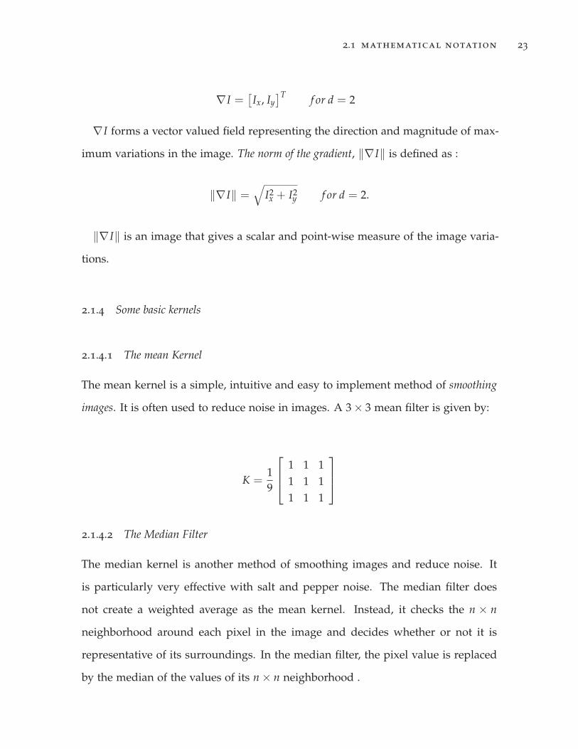
The mean kernel is a simple, intuitive and easy to implement method of smoothing
images. It is often used to reduce noise in images. A 3 × 3 mean filter is given by:
K =19
⎡⎢⎣ 1 1 1
1 1 11 1 1
⎤⎥⎦
2.1.4.2 The Median Filter
The median kernel is another method of smoothing images and reduce noise. It
is particularly very effective with salt and pepper noise. The median filter does
not create a weighted average as the mean kernel. Instead, it checks the n × n
neighborhood around each pixel in the image and decides whether or not it is
representative of its surroundings. In the median filter, the pixel value is replaced
by the median of the values of its n × n neighborhood .

2.1 mathematical notation 24
2.1.4.3 The Gaussian Kernel.
This kernel is based on the zero mean Gaussian distribution with standard devia-
tion σ:
Gσ (x, y) =1
2πσe−
x2+y2
2σ2 = Gσ(x)Gσ(y). (2.1.1)
This is a 2D convolution operator that in image processing it is used to "blur"
images, and remove detail and noise. The operator in (2.1.1) has a special property
that it is separable, that is, it can be expressed as the convolution of two 1-D ker-
nels. Thus, the 2-D convolution can be performed by first convolving the image
with a 1-D Gaussian in the x direction, and then convolving with the trasposed
1-D Gaussian in the y direction. In theory, the Gaussian distribution is non-zero
everywhere, which would require an infinitely large convolution kernel, but in
practice the kernel is effectively zero more than about six standard deviations from
the mean, and so it is truncated at this point [42]. An alternative is to truncate it
using a threshold, a small value as 0.0001 or less is used, see Figure 2.1.2. Those
kernels are normalized by the sum of the absolute vale of its entries so the kernel
sum to one.
2.1.4.4 Derivative of a Gaussian kernel
The derivatives of the Gaussian kernel in the x and y−direction are calculated
based on the derivative of the continuous Gaussian distribution. The derivative of
the Gaussian kernel in the x and y−direction will be denoted for simplicity by Gx
and Gy instead of (Gσ)x and (Gσ)y. They are defined as follows:
Gx (x, y) = − x2πσ3 e−
x2+y2
2σ2 = − xσ2 G (x, y)
and

2.1 mathematical notation 25
Figure 2.1.2: Gaussian distribution Gσ and its discrete approximation. (a) Gaussian dis-tribution Gσwith standard variation σ = 1. Approximation obtained aftertruncating Gσ at 1 × 10⁻⁴, producing a 9 × 9 Gaussian kernel Kσ for σ = 1.
Gy (x, y) = − y2πσ3 e−
x2+y2
2σ2 = − yσ2 G (x, y)
Its second derivatives are given by:
Gxx (x, y) =(x2 − σ2)
σ4 G (x, y) , Gyy (x, y) =(y2 − σ2)
σ4 G (x, y)
and
Gxy (x, y) =xyσ4 G (x, y)
As with the Gaussian convolution, these filters are also truncated. They are
separable and symmetric. So, to calculate the derivatives of the Gaussian filter in
direction x and y, it is sufficient to calculate one. The other derivative is calculated
as the transpose of the one calculated

2.2 definition of tensor 26
Figure 2.1.3: Derivatives of the Gaussian kernel in x and y−direction. (a) Plot of thex−derivative of the Gaussian distribution; (b) 2D Gx, the x−derivative of theGaussian kernel. (c)Plot of the y−derivative of the Gaussian distribution; (b)2D Gy, the y−derivative of the Gaussian kernel.
2.1.4.5 The smoothed gradient.
The smoothed gradient of a scalar image I is defined as :
∇Iσ = ∇ (Gσ ∗ I) = ∇Gσ ∗ I (2.1.2)
This definition is possible since the gradient is linear and translation invariant so
it can be represented by a convolution. Then the associativity property of convolu-
tion can be used.
2.2 definition of tensor
In this thesis, the term tensor will be used to designate a symmetric and positive
semi-definite matrix. In image processing, these particular matrices take this name
for their association to the diffusion tensor [12]. It is important not to confuse them
with the multidimensional arrays from multi-linear algebra [49]. They can also be
classified as a symmetric second order tensor in Tensor Analysis. For more details
see [50]. The definition of a tensor has some important properties. Symmetry guar-

2.2 definition of tensor 27
antees invariance to rotations and at the same time assures that all the eigenvalues
of the matrix are real valued. The positive semi definiteness guarantees that all
of them are non-negative. Mathematically they are summarized in the following
definition:
Definition 1. Let Sd+the space of all d × d tensors, this is, symmetric, positive semi-
definite matrices. T =(tij) ∈ Sd
+then,
T is symmetric if and only if for all i, j ∈ [1, d], tij = tji
T is positive semi-definite if and only if for all a ∈ Rd, aTTa ≥ 0.
The definition of tensor provides special properties for the eigenvalues μk and
eigenvectors vk of T, such as:
T is real and symmetric if and only if vk form an orthonormal vector basis in Rd. This
means that for all k, l ∈ [1, d],
vk · vl = δkl =
⎧⎪⎨⎪⎩
1 i f k = l
0 i f k �= l
T is positive semi-definite if and only if for all k ∈ [1, d], vk ≥ 0.
Therefore T may be written as:
T = RDRT (2.2.1)
where D ∈ Rd×dis a diagonal matrix of the eigenvalues μk,
D = diag (μ1, ..., μd) =
⎡⎢⎢⎢⎢⎢⎢⎢⎢⎢⎣
μ1 0 · · · 0
0 . . . . . . ...
... . . . μd−1 0
0 · · · 0 μd
⎤⎥⎥⎥⎥⎥⎥⎥⎥⎥⎦

2.2 definition of tensor 28
Figure 2.2.1: Ellipsoidal representation of a 3D tensor. Ellipsoid with axis (a) μ1 � μ2 > μ3(b) μ1 ≈ μ2 � μ3 (c) μ1 � μ2 ≈ μ3 (d) μ1 ≈ μ2 ≈ μ3. Taken from [52]
and it has determinant, det (R) = 1. R provides the orientation and D the diffusivities
of the tensor T. Note that this decomposition is known as principal component
analysis
2.2.1 Some Geometrical interpretations
From (2.2.1) T can be expressed using its eigen-decomposition as:
T =d
∑k=1
μkvkvTk (2.2.2)
μi are the eigenvalues providing the average contrast along the eigenvectors, vi for
i = 1, ..., m. Note that the eigenvalues μk of T, and the corresponding eigenvec-
tors vk, k = 1, ..., m summarize the distribution of gradient directions within the
neighborhood of a pixel p [51].

2.2 definition of tensor 29
2.2.1.1 Tensor as ellipsoids
A simple geometrical interpretation of the eigen-decomposition (2.2.2) of tensor T
is as an ellipsoid where the semi-axes are equal to the eigenvalues and directed
along their corresponding eigenvectors [53].
2.2.1.2 Tensor as a sum of weighted elementary orthogonal tensors
An interpretation, see [12], of the eigen-decomposition (2.2.2) is that T can be con-
sidered as the sum of weighted elementary orthogonal tensors(vkvT
k)[12]. Since the vk
are an orthonormal basis, then the d eigenvalues of(vkvT
k)
are : 1 for some eigen-
vector vk and 0 for the other d− 1 eigenvectors perpendicular to vk. The elementary
tensors(vkvT
k)
can be viewed as thin ellipsoids with one axis of length 1 and the
others of length 0. In that form they represent the orientation of the tensor. A whole
tensor T is simply a combination of these (weighted) orthogonal orientations [12].
If for all k ∈ [1, d] the eigenvalues μk of T are equal to a constant μ then:
T =d
∑k=1
μvkvTk = μIdd.
where Idd is the d × d identity matrix. in this case, T does not have a preferred
diffusion direction and it is independent of the orientation. So, T describes isotropic
structures and it is visualized as a sphere with a radius μ. The corresponding diffu-
sion process is done with the same weight in all the directions of the space.
2.2.1.3 Tensor as encoder of the local structure-Case 2-D and 3-D
Another way to visualize the geometrical representation of the eigen-decomposition
(2.2.2) of T is known as glyphs developed by Wiklund in [54]. Glyphs depict tensor
variables by mapping the tensor eigenvectors and eigenvalues to the orientation
and shape of a geometric primitive, such as a cuboid or ellipsoid [55]. They are

2.2 definition of tensor 30
Figure 2.2.2: Representation of basic local structures of a tensor T ∈ R2×2, using ten-sor glyphs. (a) Linear structure when T1 is dominant, vectors v1, v2 arethe eigenvectors to the eigenvalues μ1 = 1, μ2 = 0.1 respectively. Right:Isotropic structure when T2 is dominant, for this case the eigenvalues areμ1 = 0.67, μ2 = 0.63 and have the same eigenvalues as in (a). This figure wasrendered using the tensor visualization tool T-FLASH [54].
commonly used to represent the state of a tensor field point-wise and their col-
lective behavior, when e.g. arranged in a grid, help to gain an intuition on the
change of shape and orientation of the tensors [56]. Ellipses are used for d = 2
or d-dimensional ellipsoids for d > 2. The eigenvectors becomes the axis of the
ellipsoids and the eigenvalues its magnitude, see Figure2.2.2. The difference with
the other ellipsoid representation is that the structures for all eigenvectors are color
coded. So in one representation it is depicted the behavior of all eigenvalues and
eigenvectors independently and in the same ellipsoid.
When the dimension of the tensor is d = 2, then from (2.2.2) the tensor T can be
written as:
T = μ1v1vT1 + μ2v2vT
2 , μ1 ≥ μ2 (2.2.3)

2.2 definition of tensor 31
After some algebra manipulations,T can be decomposed into two parts: A linear
part T1 and the isotropic part T2 as
T = T1 + T2,
where
T1 = (μ1 − μ2)v1vT1 , (2.2.4)
T2 = μ2(v1vT1 + v2vT
2 ). (2.2.5)
This decomposition help us interpret and visualize the relative contributions of
the basic local structures: Linear and isotropic [54]. Figure 2.2.2 shows the tensor
glyph for each case. Figure 2.2.2(a) shows a tensor T where the linear local part,
T1, is dominant. T1 is visualized as a red spear whose length is proportional to the
magnitude of T1, see (2.2.4). The yellow circle shows the isotropic part, T2. Figure
2.2.2(b) shows T when T2 is dominant μ1 ≈ μ2 and it is visualized as a yellow circle
with radius μ = μ2. In this case the linear part T1has magnitude μ1.
For the three dimensional case d = 3, T is decomposed as:
T = μ1v1vT1 + μ2v2vT
2 + μ3v3vT3 , μ1 ≥ μ2 ≥ μ3 (2.2.6)
In the same way as for the 2D case, T can be decomposed as the contribution of
three basic local structures, this is:
T = T1 + T2 + T3
T1 describe the linear structures, T2 the planar structures and, T3 the isotropic
structures. They are defined as [54]:
2.2 definition of tensor 32
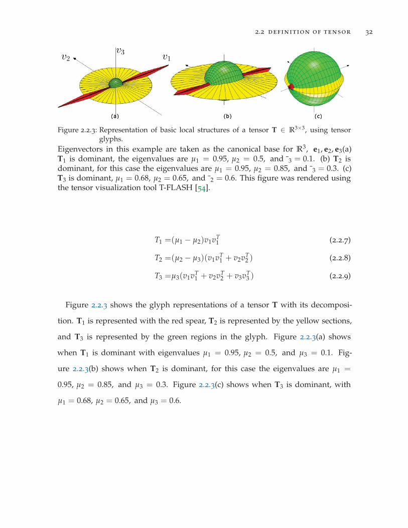
Figure 2.2.3: Representation of basic local structures of a tensor T ∈ R3×3, using tensorglyphs.
Eigenvectors in this example are taken as the canonical base for R3, e1, e2, e3(a)T1 is dominant, the eigenvalues are μ1 = 0.95, μ2 = 0.5, and ¯3 = 0.1. (b) T2 isdominant, for this case the eigenvalues are μ1 = 0.95, μ2 = 0.85, and ¯3 = 0.3. (c)T3 is dominant, μ1 = 0.68, μ2 = 0.65, and ¯2 = 0.6. This figure was rendered usingthe tensor visualization tool T-FLASH [54].
T1 =(μ1 − μ2)v1vT1 (2.2.7)
T2 =(μ2 − μ3)(v1vT1 + v2vT
2 ) (2.2.8)
T3 =μ3(v1vT1 + v2vT
2 + v3vT3 ) (2.2.9)
Figure 2.2.3 shows the glyph representations of a tensor T with its decomposi-
tion. T1 is represented with the red spear, T2 is represented by the yellow sections,
and T3 is represented by the green regions in the glyph. Figure 2.2.3(a) shows
when T1 is dominant with eigenvalues μ1 = 0.95, μ2 = 0.5, and μ3 = 0.1. Fig-
ure 2.2.3(b) shows when T2 is dominant, for this case the eigenvalues are μ1 =
0.95, μ2 = 0.85, and μ3 = 0.3. Figure 2.2.3(c) shows when T3 is dominant, with
μ1 = 0.68, μ2 = 0.65, and μ3 = 0.6.

2.2 definition of tensor 33
2.2.2 Classification of local neighborhoods
The classification of the eigenvalues of the structure tensor produce very valuable
information. The following classification will be based on the rank of the matrix of
eigenvalues.
2.2.2.1 Classification of local neighborhoods: 2-D Case
The classification of local neighborhoods is done by finding the null space, that is,
by looking for eigenvalues that are zero. If the gray values in the direction of an
eigenvector vk do not change then μk = 0. The analysis of the eigenvalues for two
dimensional and 3 dimensional cases will be presented and aided with results in
Section 2.2.1.3. T1 and T2 are defined as in (2.2.4) and (2.2.5) respectively.
1. μ1 = μ2 = 0, rank 0 tensor. This is the null tensor, T = 0. The square Frobe-
nious norm of the gradient μ21 +μ2
2 is zero. In this case, the local neighborhood
has constant values. It belongs to an object with a homogeneous feature;
2. μ1 > μ2 = 0, rank 1 tensor. In this case, T2 = 0 and T1 is dominant, so this
tensor describes linear structures. In an image that could either be the ideal
edge (without noise) of an object or an oriented texture;
3. μ1 ≥ μ2 > 0, rank 2 tensor. There are several distinctive sub-cases to this case.
• μ1 = μ2, In this case T1 = 0 and T2 is dominant, so this tensor describes
an isotropic structure, i.e., it changes equally in all directions, see Figure
2.2.2(b).
• μ1 � μ2 ≈ 0. This is still a rank 2 tensor. This case describe a noisy edge
or a noisy oriented texture, as shown in Figure 2.2.2(a). This is the most
common case of edges on images extracted from sensors.

2.2 definition of tensor 34
2.2.2.2 Classification of local neighborhoods: 3-D Case
To describe the analysis of the classification of the eigenvalues in three dimensions,
T1, T2 and T3 will be used and defined as in (2.2.7), (2.2.8) and (2.2.9) respectively.
Some of the neighborhoods are extension of the two dimensional case.
1. μ1 = μ2 = μ3 = 0, rank 0 tensor. There is neither a preferred orientation of
signal variation nor significant variation, which corresponds to homogeneous
regions [57].
2. μ1 > μ2 = μ3 = 0, rank 1 tensor. T1 is dominant with coefficient equal to μ1,
T2 and T3 are equal to zero. The signal values change only in the direction
of v1. The neighborhood includes a boundary between two objects (surface)
or a layered texture [58]. Using the glyph representation, this will look like
Figure 2.2.2(a) but in 3D ;
3. μ1 ≥ μ2 > μ3 = 0, rank 2 tensor. In the general case, The signal values, i.e.,
gray values in the image, change in two directions which generate a plane,
and are constant in a third. v3 gives the direction of the constant gray values.
Using the glyph representation this will look like Figure 2.2.3(a) but without
the green region ;
• μ1 ≈ μ2 > μ3 = 0, T1 ≈ 0, T3 = 0 and T2 is dominant with coefficient
equal to μ2. This happens at the edge of a three-dimensional object in a
volumetric image [58]. Using the glyph representation this will look like
Figure 2.2.3(b) but without the green region.
4. μ1 ≥ μ2 ≥ μ3 > 0, rank 3 tensor. There is no preferred orientation of signal
variation. This is, the gray values change in all three directions. In the general
case, the glyph representation this will range from Figure 2.2.3(a) to (c) any
of those cases can happens. An special case to that is:

2.3 structure tensor 35
• μ1 ≈ μ2 ≈ μ3 > 0, T3 is dominant with coefficient equal to μ3. The
signal variation is equal in all directions. This case represents a corner
or a junction in 3D or a region with isotropic noise [57, 58]. The glyph
representation is given by Figure 2.2.3(c).
In practice, it will not be checked whether the eigenvalues are zero but below
a critical threshold that is determined by the noise level in the image. Note that
this tensor is suitable to distinguish very well structures that result from signal
variation in one direction.
2.3 structure tensor
The structure tensor in this work will refer to the local structure tensor, that is, the
structure tensor defined in a neighborhood. In images, tensors are better suited
to find structures inside of a neighborhood in which the gray value only changes
in one direction, known as simple local neighborhood [59]. In these neighborhoods,
oriented structures are formed since the gray values are constant along lines. This
property of a neighborhood is known as local orientation [58].
2.3.1 Directions vs. orientation
The direction is defined over the full angle range of 2π (360°). Orientation will
be used where the angles has range of π (180°). This distinction is done since
two patterns that differ by an angle of π are indistinguishable inside a simple
neighborhood. On the other hand, two vectors that point in opposite directions,
i.e., differ by 180°, are different. An example of this is the gradient vector that

2.3 structure tensor 36
always points in the direction where the gray values are increasing. Thus, the
direction of a simple neighborhood is different from the direction of a gradient.
2.3.2 Estimation of the Local Structure Tensor
The methods used to estimate the local structure tensor can be classified as:
• Gradient methods: These methods use the spatial gradient to determine the
signal orientation [11, 10, 8, 60].
• Local-energy method: This tries to find a representation of the orientation
based on the local energy method. The energy of the signal is quantified using
quadrature filters then the local structure is determined. These methods are
less related to our work and will not be presented here. They are based on
the work of Knutsson and his group [59, 61, 62, 63, 64].
2.3.3 Structure Tensor: The development of Gradient Based methods
The development of the structure tensor in image processing was driven by the
problem of finding the optimal local orientation in a neighborhood [58, 65, 66] and
the problem of defining an edge in multichannel images [67].
2.3.3.1 Optimization Problem
In this framework [58, 65, 66], The structure tensor results from the solution of an
optimization strategy to determine the orientation of a neighborhood; to find the
orientation that shows the least deviation from the directions of the gradient. Then
the idea is to maximize the squared scalar product between the gradient vector

2.3 structure tensor 37
g = ∇I (p′) and the unit vector representing the local orientation, r, of an image
patch centered at location p:
maximize(
gTr)2
= maxθ
[∣∣∣gT∣∣∣2 cos2 (θ)
], θ = ∠ (g, r) . (2.3.1)
The maximum in (2.3.1) is found where g and r are parallel or anti-parallel, θ = 0◦
or θ = 180◦ respectively. The following integral is maximized in a local neighbor-
hood of a point p, denoted by N (p), where p ∈ Ω :
maxp′∈N (p)
ˆw(
p − p′) (
gTr)2
dp′ (2.3.2)
where the window function w determines the size and shape of the neighborhood
around a point p in which the orientation is averaged. The maximization problem
must be solved for each point p. In vector notation, (2.3.2) is:
max(
rT Jr)
(2.3.3)
with
J =ˆ ∞
−∞w(
p − p′) (
g(
p′)
g(
p′)T)
dp′.
Note that J is the convolution of the window function w with the outer product of
the gradient
g(
p′)= ∇I
(p′)= [Ix1 , · · · , Ixd ],
where Ixi =∂I∂xi
, for i = 1, ..., d and d is the dimension of the neighborhood, then J
can be expressed as:
J = w ∗ (∇I(
p′)∇I
(p′))
(p) .
In matrix representation, this is:

2.3 structure tensor 38
J =
⎡⎢⎢⎢⎢⎢⎣
(w ∗ I2
x1
)(p) · · · (w ∗ Ix1 Ixd) (p)
... . . . ...
(w ∗ Ixd Ix1) (p) · · ·(
w ∗ I2xd
)(p)
⎤⎥⎥⎥⎥⎥⎦ . (2.3.4)
It is straightforward to extend the tensor for multichannel signals as:
J =m
∑i=1
⎡⎢⎢⎢⎢⎢⎣
(wi ∗ I2
x1,i
)(p) · · · (wi ∗ Ix1,i Ixd,i
)(p)
... . . . ...(wi ∗ Ixd,i Ix1,i
)(p) · · ·
(wi ∗ I2
xd,i
)(p)
⎤⎥⎥⎥⎥⎥⎦ .
The weighting function w might be different for each channel in order to consider
the significance and spatial resolution of a certain channel [58]. A tensor is an
adequate first-order representation of a local neighborhood since it only involves
first-order derivatives. It is important to note that this tensor only analyzes in
which direction(s) the signal variations occur. This is, where the gray values change.
More complex structures such as structures with multiple orientations cannot be
distinguished.
The problem of maximize (2.3.3), subject to rTr = 1, can be solved by using a
Lagrange multiplier μ and finding the extremes of
μ(
1 − rTr)+ rT Jr. (2.3.5)
Differentiating with respect to r, and setting the derivative equal to zero results in
an eigenvalue problem.
Jr = μr (2.3.6)

2.3 structure tensor 39
This is the problem of finding for which values of μ (2.3.6) has a nonzero solution,
i.e., the eigenvalues of J. Substitution in (2.3.5) shows that the solution is the
eigenvector corresponding to the largest eigenvalue, μ1. Then the structure tensor
is J with the window function defined by the Gaussian distribution in (2.1.1) and
standard deviation ρ. For the discrete case, a Gaussian kernel it is used, see Section
2.1.4.3.
2.3.3.2 Structure tensor as a covariance matrix
From a statistical point of view, when signals are regarded as random fields an
interesting relationship can be established between the local structure tensor and
the covariance matrix Cov.
Cov = J − E {∇I (p)} E{∇I (p)T
}
where E {·} is the expectation operator and J and ∇I (p) are defined as in Section
2.3.3.1. Cov and J are equal when E {∇I (p)} = 0. For example on homogeneous
areas such as in neighborhood with planes or lines shape, E {∇I (p)} = 0, i.e.,
E {Ix1} = 0 and E {Ix2} = 0. In those areas, if the dimension of the image is d = 2
(scalar or vector valued) and the window function w in (2.3.4) is Gσ a Gaussian
with variance σ2 then the structure tensor can be modeled as the joint distribution
of the two partial derivatives, Ix1 and Ix2 . This is,
J =
⎡⎢⎣ Gρ ∗
(I2x1
)Gρ ∗ (Ix1 Ix2)
Gρ ∗ (Ix1 Ix2) Gρ ∗(
I2x2
)⎤⎥⎦ =
⎡⎢⎣ E
{I2x1
}E {Ix1 Ix2}
E {Ix1 Ix2} E{
I2x2
}⎤⎥⎦ = Cov (Ix1 , Ix2)
The convolution corresponds to computing the expectation value with regard to a
weighting of the derivatives according to their distance from p.

2.3 structure tensor 40
2.3.3.3 Using Differential Geometry
This definition is motivated by finding a definition for an edge in a vector valued
image. This framework was presented by Di Zenzo in [67]. The idea is to define
a gradient based edge detector for vector-valued images such that the edge infor-
mation along a given direction in one channel reinforces the edge evidence of the
other channels. This is not the only way to do this extension and another definition
can lead us to a different framework. Given two pixels p and q in the image f
with f (p) and f (q) ∈ Rm. d f = f (p)− f (q) approximates the arc length when
dist(p, q) → 0, where dist is the Euclidean distance. Therefore,
d f =2
∑i=1
∂ f∂xi
dxi (2.3.7)
and its square Euclidean norm is given by
‖d f ‖2 =2
∑i,j=1
∂ f∂xi
∂ f∂xj
dxidxj = dxT
(∑
l∇ fl∇ f T
l
)dx (2.3.8)
‖d f ‖2 describes the rate of change of the values (i.e.,intensity or radiance) in the
image. Its extremes are along the direction given by the eigenvectors of maximum
and minimum change, v1, v2 respectively, of the tensor
J = ∑j∇ f j∇ f T
j . (2.3.9)
The magnitude of the extremes are given by μ1 and μ2, the largest and smallest
eigenvalues of J respectively.

2.3 structure tensor 41
Figure 2.3.1: Smoothed Gradient vs. Structure Tensor. Fingerprint image of size 227 × 227.(a) Original image. (b) Gradient orientation �� = 0.5. (c) Gradient orientation�� = 2.5. (d) Structure Tensor Orientation given by ω2 with �� = 0.5, � = 4.
2.3.4 Scalar structure tensor
Finding the local structure of each pixel requires considering the data of its neigh-
borhood [13], which introduces the concept of the structure tensor. The task of
knowing if a pixel is part of an edge or a corner cannot be accomplished with only
its gradient information. There is a need to know if the pixel is similar to its neigh-
bors or not and in which direction. Therefore, the incorporation of its neighbors’
gradient information is required.
The local spatial neighborhood information becomes more important when the
data is corrupted by noise since the structure has to be estimated in the presence of
unreliable data. To incorporate the information within a neighborhood of a pixel,
Gaussian convolution with variance ��2, see Section 2.1.4.3, is used on the original
image producing a smoothed image, i.e.,
Iσ = Gσ ∗ I. (2.3.10)
This convolution is used to weight the structure information of each pixel’s neigh-
bors. It is also used to regularize the structure tensor and make it robust to noise.

2.3 structure tensor 42
For simplicity in notation, Ix and Iy will be used though this work instead of (Iσ)x
and (Iσ)x as the horizontal and vertical derivatives of the smoothed image, Iσ, re-
spectively. The problem with the smoothed gradient, ∇Iσ = [ Ix Iy ]T, is that it
can suffer cancellation effects. Figure 2.3.1(b)-(c) illustrates the gradient orientation
using gray values where vertical gradients are depicted in black and horizontal
ones in white. The gradient orientation is defined as tan−1 (Iy/Ix). If �� is small as
in (b), then high fluctuation of the orientations remains. As �� gets larger, as in (c),
then it becomes useless since neighboring gradients with the same orientation but
with opposite signs (direction) cancel one another. To avoid that effect, the outer
product of the smoothed gradient, which is a symmetric, positive semi-definite
matrix, is considered in the structure tensor and known as the initial matrix field
[66]:
J0 = ∇Iσ∇ITσ =
⎡⎢⎣ I2
x Ix Iy
Ix Iy I2y
⎤⎥⎦ . (2.3.11)
Its eigenvalue decomposition is given by:
J0 =
[ω1 ω2
] ⎡⎢⎣ μ1 0
0 μ2
⎤⎥⎦ [ ω1 ω2
]T
where ω1 ‖ ∇Iσ and ω2 ⊥ ∇Iσ. It is important to note that ∇Iσ �= ∇I for σ > 0.
So, ω1 ∦ ∇I. μ1 = |∇Iσ|2 = Ix and μ2 = 0.
Then the structure tensor for a neighborhood of scale ρ is computed with a smooth-
ing step performed by a convolution of the components of with a Gaussian kernel
Gρ , which is known as the local integration step, as follows
Jρ = Gρ ∗ J0 =
⎡⎢⎣ Gρ ∗ J011 Gρ ∗ J012
Gρ ∗ J021 Gρ ∗ J022
⎤⎥⎦ =
⎡⎢⎣ a b
b c
⎤⎥⎦ (2.3.12)

2.3 structure tensor 43
Its eigen-decomposition is given by:
Jρ =
[v1 v2
] ⎡⎢⎣ μ1 0
0 μ2
⎤⎥⎦ [ v1 v2
]T,
where
v1 ‖
⎛⎜⎝ 2b
c − a +√(a − c)2 + 4b2
⎞⎟⎠ and v2 ⊥ v1
and the corresponding eigenvalues μ1 and μ2 given by
μ1 =a + c +
√(a − c)2 + 4b2
2and μ2 =
a + c −√(a − c)2 + 4b2
2
Figure 2.3.1(d) shows eigenvector v2, which defines the coherence orientation or
the structure tensor orientation for the fingerprint image. Figure 2.3.1(d) is the
desired average orientation of the lines (compare with Figure 2.3.1(b)). In Figure
2.3.1(d) the fingerprint singularity (minutiae) is well described.
2.3.5 Vector-Valued Structure Tensor
For the vector-valued image with m bands, the structural information from all
channels, encoded in the initial matrix field, is coupled with a fusion step, which is
usually a sum over all channels. To make the structure tensor independent of the
number of channels, an average is calculated, i.e., all channels are weighted equally.
In this case, the initial matrix field for the vector valued case is given by:
J0 =1m
m
∑i=1
J0i =1m
⎡⎢⎢⎢⎣
m
∑i=1
I2x,i
m
∑i=1
Ix,i Iy,i
m
∑i=1
Ix,i Iy,i
m
∑i=1
I2y,i
⎤⎥⎥⎥⎦ (2.3.13)

2.4 image processing using geometrical pdes 44
Then the structure tensor for a neighborhood of scale ρ is computed as in the
scalar case, Gρ is a Gaussian of variance ρ
Jρ = Gρ ∗ J0. (2.3.14)
and its eigen-decomposition is given by:
Jρ =
[ω1 ω2
] ⎡⎢⎣ μ1 0
0 μ2
⎤⎥⎦ [ ω1 ω2
]T. (2.3.15)
2.4 image processing using geometrical pdes
A general review of main contributions in image processing using Partial Differen-
tial Equations (PDEs) in vector valued images and a review of anisotropic process-
ing of images using divergence-driven PDEs are presented.
PDEs in image processing have been researched and used since 1960 [68]. But
around 1990, as a result of a huge interest from scientists around the world, well
founded mathematical and numerical methods for PDEs applied to image process-
ing, in particular gray level images, were developed. As a consequence, many
faster and efficient algorithms emerged. Processing vector-valued data has become
an active research area because of the wider use of instruments that produce vector-
valued data and its usage in many fields and applications. Also cheaper computer
memory and some new computer architectures have helped to adapt, modify and
create new algorithms and methods for this particular kind of data. Some advan-
tages of using PDEs in processing vector-valued Images are [2]:
• A wide and robust mathematical theory of PDEs.
• Efficient and reliable numerical methods to solve PDEs.

2.4 image processing using geometrical pdes 45
• Theory and methods are generalizable to higher dimensions.
• Many of these methods are related to well known physical phenomena such
as conservation, diffusion, etc.
Images, in general, result from a uniform sampling of a 2D or 3D signal done by
sensors so they are discontinuous by nature. On the other hand, PDE-based image
processing theory is developed primarily assuming continuity. Therefore, there is
a need for discretization techniques to approximate a solution of the PDEs in this
kind of data. The discretization uses a mesh that subdivides the image domain to
numerically integrate over each element in the mesh. Since the mesh is determined
by the sampling of the pixels in the image, the discretization is restricted to use a
structured rectangular mesh without refinement.
2.4.1 Physical background of diffusion
The physical concept of diffusion can be found in electromagnetic theory, fluid
dynamics, quantum mechanics, and so on. It will be presented in this section in
the context of the physical phenomenon of mass transport. Diffusion can be seen
as the process that equilibrates concentration of differences without creating or
destroying the mass [69]. This equilibrium property is given by Fick’s first law:
j = −D · ∇u.
The flux j compensates for a concentration gradient ∇u. The relation of j and ∇u
is given by the diffusion tensor D, which is a symmetric positive definite matrix. The
term tensor in this case is used to describe those kinds of matrices, not in the wider
sense as in Physics [3]. Isotropic diffusion is known as the case where j and ∇u are

2.4 image processing using geometrical pdes 46
parallel and anisotropic diffusion if j and ∇u are not. This is the definition adopted
by Weickert [2].
Since diffusion only transports mass without destroying it or creating new mass,
dmdt = 0, where t denotes time. Application of Reynolds’ transport theorem and
Gauss’ divergence theorem leads to a differential coordinate-free form of the conti-
nuity equation
∂tu + div(j) =dmdt
= 0.
To adapt this form to a specific coordinate system, just provide a expression of
the divergence operator in that particular coordinate system. Then by substituting
Fick’s flux into the continuity equation, the diffusion equation [69, 70] is obtained .
∂tu = div(D · ∇u). (2.4.1)
Equation (2.4.1) is a conservation law that appears when modeling many physical
transport phenomena. In general, these processes involve mass or energy transport
in a conductive media, without sources or sinks [69]. In the context of image pro-
cessing, the mass concentration is interpreted as the intensity of the image signal at
a certain location. The diffusion direction will change depending on the diffusion
tensor D. If D is constant in the whole image domain is known as Homogeneous
diffusion and a space-dependent filtering is called inhomogeneous. A diffusion filter
is called nonlinear if the diffusion tensor is a function of the differential structure of
the evolving image itself, and linear diffusion if it does not depend on it [70].
In image processing, there is no real evolution in time, the variable n is a dummy
variable that simulates an iterative process as n is gradually increases from n = 0
in which ui(x, 0) = fi(x) is the original image. Some diffusion processes produce a
family {Tt f |t ≥ 0} of gradually smoother versions of f which is known as scale-
space, see Figure 2.4.1. For a study on scale spaces see [45, 71, 72] and references

2.4 image processing using geometrical pdes 47
Figure 2.4.1: Scale-space produced by coherence-enhancing diffusion in a thyroid tissue.σ = 0.5, ρ = 4, Ω = (0, 252)2 k = 0.1.(a) Original Image (b)n = 10; (c) n = 15;(d) n = 20; (e) n = 30; (f) n = 40; (g) n = 50; (h) n = 100; (i) n = 200.
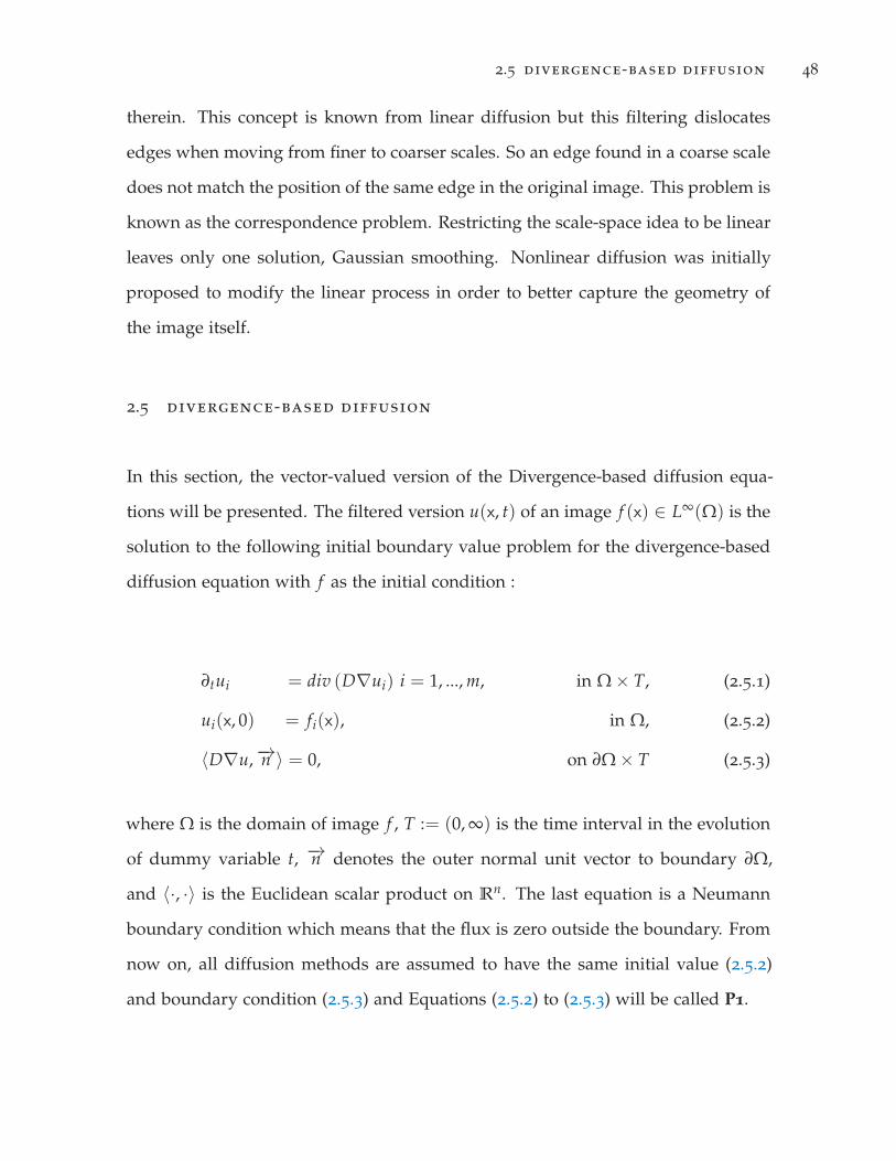
2.5 divergence-based diffusion 48
therein. This concept is known from linear diffusion but this filtering dislocates
edges when moving from finer to coarser scales. So an edge found in a coarse scale
does not match the position of the same edge in the original image. This problem is
known as the correspondence problem. Restricting the scale-space idea to be linear
leaves only one solution, Gaussian smoothing. Nonlinear diffusion was initially
proposed to modify the linear process in order to better capture the geometry of
the image itself.
2.5 divergence-based diffusion
In this section, the vector-valued version of the Divergence-based diffusion equa-
tions will be presented. The filtered version u(x, t) of an image f (x) ∈ L∞(Ω) is the
solution to the following initial boundary value problem for the divergence-based
diffusion equation with f as the initial condition :
∂tui = div (D∇ui) i = 1, ..., m, in Ω × T, (2.5.1)
ui(x, 0) = fi(x), in Ω, (2.5.2)
〈D∇u,−→n 〉 = 0, on ∂Ω × T (2.5.3)
where Ω is the domain of image f , T := (0, ∞) is the time interval in the evolution
of dummy variable t, −→n denotes the outer normal unit vector to boundary ∂Ω,
and 〈·, ·〉 is the Euclidean scalar product on Rn. The last equation is a Neumann
boundary condition which means that the flux is zero outside the boundary. From
now on, all diffusion methods are assumed to have the same initial value (2.5.2)
and boundary condition (2.5.3) and Equations (2.5.2) to (2.5.3) will be called P1.

2.5 divergence-based diffusion 49
2.5.1 Linear diffusion
The differences between divergence-based methods is D. If D is a constant, then
2.5.1 is:
∂tui = Δui i = 1, ..., m, in Ω × T,
the solution using the homogeneous diffusion process is [68]:
ui(x, t) =
⎧⎪⎨⎪⎩
fi(x) t = 0(G√
2t ∗ f)(x) t > 0
which is the convolution of the image with the Gaussian filter G√2t.
2.5.2 Perona and Malik Isotropic nonlinear diffusion
Perona and Malik [73] in 1990 presented the first nonlinear diffusion method that
work in images. For that reason, it is considered as a historical work. This was the
first adaptive smoothing method, which is based on the idea of applying a process
which itself depends on local properties of the image. This process is given by
(2.5.1) in which D is the diffusivity function g given by:
g(s2) =1
1 + s2/λ, λ > 0. (2.5.4)
with s2 =1
m ∑j∥∥∇uj
∥∥2 j = 1, ..., m, λ can be set as a percentile P of the image
gradient magnitudes at each iteration. Perona and Malik recommended the value
P = 90% [73]. Equation (2.5.1) is solved using a finite difference discretization
scheme. This filter was motivated by the idea of adapting the diffusivity g to the

2.5 divergence-based diffusion 50
gradient of the actual image u(x, t) instead of the original image f (x) introducing
feedback in the process which leads to nonlinear diffusion. In 1993, Alvarez [74]
showed that there exist PDEs with the original image as the initial condition that
govern scale-spaces which satisfy some architectural, information-reducing, and
invariance properties. They showed that Perona-Malik diffusion was ill-posed and
produced sharpening of edges if the gradient is larger than λ. In practice, the
method behaves better than predicted by theory. Latter was shown in [70] that the
standard finite difference scheme brought some regularization and that was part of
the reason it worked. In 1993, Catte et al [72] showed in an elegant mathematical
formulation that the Perona-Malik model could be regularized by replacing the
diffusivity g
⎛⎜⎝ 1
m ∑j∥∥∇uj
∥∥2
⎞⎟⎠ by g
⎛⎜⎝ 1
m ∑j∥∥∇uσ,j
∥∥2
⎞⎟⎠ with
uσ,j := Gσ ∗ uj, for j = 1, ..., m
where Gσ(x) is defined as in Section 2.1.4. They also showed existence, unique-
ness, and regularity of a solution to the initial and boundary value problem. This
regularization worked in part since Gaussian smoothing is a low-pass filter that
attenuates, in a monotone way, high frequencies. So (2.5.1) becomes
∂tui = div
⎛⎜⎝g
⎛⎜⎝ 1
m ∑j
∥∥∇uσ,j∥∥2
⎞⎟⎠∇ui
⎞⎟⎠ , for i = 1, ..., m. (2.5.5)
σ will take care of the case when high oscillation in the data can be misinterpreted
as edges, and it is viewed as a noise parameter. The diffusivity g(s2) is a mono-
tonically decreasing function of its argument and the flux Φ = g(s2)s is mono-
tonically non-decreasing in s. This last condition is required in order to ensure
well-posedness in the nonlinear setting using classical frameworks [21].

2.5 divergence-based diffusion 51
2.5.3 Tensor Anisotropic nonlinear diffusion
Nonlinear isotropic diffusion uses a scalar diffusivity g which is adapted to the
geometry of the image. Anisotropic diffusion uses a diffusion tensor D. The ad-
vantage of using this tensor is that diffusion can be directed to any of its (maximum
or minimum) directions. The structure tensor when written in its eigenvalue de-
composition, see (2.3.15), can be decomposed as the sum of two expressions that
describe two basic local structures: linear and isotropic structures, see (2.2.4)-(2.2.5).
From the linear structures found using the eigenvector corresponding to the small-
est eigenvalue, oriented flow-like structures can be distinguished and enhanced
using coherence enhancement. On the other hand, regularization that preserves
edges, which consist in smoothing along edges inhibiting the diffusing across them
is done by finding the eigenvector corresponding to the largest eigenvalue of the
structure tensor.
In this section, the three most used divergence-based anisotropic diffusion meth-
ods are presented. The first model will be motivated by the extension of the dif-
fusivity function g from a scalar function to a tensor. It also gives an intuition on
how to extend this concept to design filters to enhance 1D features and denoise
preserving the edges. The second one is motivated by the necessity, in some appli-
cations, to rotate the flux towards the orientation of features of interest. A case for
this kind of filtering is the Coherence-Enhancing Diffusion (CED). This one is adapted
to process 1-D features such as lines and flow-like structures. The third one is moti-
vated as an extension to anisotropic diffusion of the Perona-Malik model. Since this
method removes noise from edges it is known as Edge-Enhancing Diffusion (EED).
CED and EED will be objects of further study.

2.5 divergence-based diffusion 52
2.5.3.1 Anisotropic extension of the isotropic model based on scalar diffusivity
An extension of a scalar valued function g(s2) by a tensor g(J) is given by:
g(J) =[
θ+ θ−
] ⎡⎢⎣g(μ2+) 0
0 g(μ2−)
⎤⎥⎦⎡⎢⎣θ+
θ−
⎤⎥⎦ (2.5.6)
where μ−, μ+ are the smallest and largest eigenvalues of J and θ−, θ+ its respective
eigenvectors. In this case, J = J0, the initial matrix field for vector valued images,
is a natural choice. Using the same diffusivity or diffusion tensor for all bands
ensures that the evolution is synchronized. g(J) will be constructed using the
process described before. An example of a diffusivity function g is given by [75]:
g(s2) = α +1√
β2 + s2. (2.5.7)
So, D = g(J) for (2.5.1). As a consequence, linear and nonlinear isotropic mod-
els can be characterized by their diffusivities g(
∑j ∇ f Tj ∇ f j
)and g
(∑j ∇uT
j ∇uj
)respectively, while its anisotropic counterparts are given by g(∑j ∇ f j∇ f T
j ) and
g(∑j ∇uj∇uTj ), j = 1, ..., m.
2.5.3.2 Coherence-Enhancing Diffusion
The basic ingredients of Coherence Enhancing Diffusion (CED) are:
• Diffusion is done in the direction of smallest variation of the structure tensor.
• A shape-adapted Gaussian smoothing in a small neighborhood around that
direction is used.
In 1993, Catte et al. [76] presented a reaction-diffusion model where the diffusion
was along the eigenvector corresponding to the smallest eigenvalue of its diffusion
tensor defined as: κ2 = g(|∇uσ|2). But this model did not produce a scale-space,

2.5 divergence-based diffusion 53
and its diffusion tensor D had eigen-directions adapted to ∇uσ,i which make them
sensible to changes in σ, see Section 2.3.4. In 1998, Weickert [2] presented an
approach that is a semi-local analysis by means of the structure tensor combined
with 1-D diffusion along one of its eigenvectors which is presented in this section.
CED is basically a 1-D diffusion, where a minimal amount of isotropic smoothing
is added for regularization purposes. For this case, D is built upon the structure
tensor Jρ defined for vector-valued images as in (2.3.14). μ = (μ1 − μ2) is a measure
of local coherence [23]. μ2 is large for anisotropic structures and tend to zero for
isotropic ones. Constant areas are characterized by μ1 = μ2 = 0, straight edges by
μ1 � μ2 = 0, and corners by μ1 > μ2 � 0 [77].
D
(1m
m
∑i=1
Jρ,i
):=
⎡⎢⎣λ β
β ν
⎤⎥⎦ =
[v1 v2
] ⎡⎢⎣κ1 0
0 κ1
⎤⎥⎦⎡⎢⎣vT
1
vT2
⎤⎥⎦ . (2.5.8)
In (2.5.8) D(·) is the diffusion tensor written as a function to emphasize its depen-
dency on the expression inside the parenthesis. To enhance coherence structures,
the process should smooth mainly along the coherence direction v2. So κ2 increases
with μ2. Using [20] functions, κ1, κ2 are given by :
κ1 = α, α ∈ (0, 1), α � 1,
κ2 = g(μ2) =
⎧⎪⎪⎪⎨⎪⎪⎪⎩
α, if μ1 = μ2,
α + (1 − α) exp(−Cμ2
), C > 0 else.

2.5 divergence-based diffusion 54
Note that by definition κ2 ∈ (0, 1). α = 10−3 is the most common value used in the
literature. α guarantees that the process never stops, and keeps the diffusion tensor
uniformly positive definite [23]. C is a threshold parameter;
if μ2 � C then κ2 ≈ 1, (2.5.9)
if μ2 � C then κ2 ≈ α. (2.5.10)
In addition, D satisfies smoothness, symmetry and uniform positive definiteness
properties [2]. The smoothness of D come from the convolution with Gσ and Gρ,
which guarantees that the elements of D are C1 functions [77].
2.5.3.3 Edge Preserving Diffusion
In this context, edge-diffusion is presented as special case of coherence-enhancing
diffusion in which the integration parameter ρ = 0. In (2.5.1), diffusion at the edges
is inhibited and as a consequence noise in the edges cannot be eliminated. To solve
this problem, the diffusion should be parallel to the edges instead of perpendicular
to them. To that end, the diffusion tensor D will depend on ∑mi=1 J0i and eigenvalues
κ1, κ2 defined as:
D
(m
∑i=1
J0i
):=[
v1 v2
] ⎡⎢⎣κ1 0
0 κ1
⎤⎥⎦⎡⎢⎣v1
v2
⎤⎥⎦ (2.5.11)
and
κ1 := g
(∑
i|∇uσ,i|2
),
κ2 := 1

2.5 divergence-based diffusion 55
Figure 2.5.1: Comparison between EED and CED. (a) Original image by Monet [78]. (b)Original image after CED n = 10, σ = 0.5, ρ = 3, ψ = 50th percentile. (c)Original image after EED,n = 10, σ = 1, ψ = 50th percentile.
If σ tends to zero, the isotropic Perona-Malik process is obtained. Many of the
edge enhancing diffusion models differ in the function g, the following function
was proposed by Weickert [2]:
g(s) :=
⎧⎪⎨⎪⎩
1, s ≤ 0;
1 − exp(
−Cm(s/λ)m
), s > 0.
(2.5.12)
The exponential function is chosen to enforce smoothness. D is positive definite
since ∇uσ,i is bounded on Ω × I and |∇uσ,i|2 > 0. Cm is calculated such that the
flux Φ(s) = g(s) · s increases for s ∈ [0, λ] and decreases for s ∈ (λ, ∞). Then the
values used are m = 4, Cm = 3.31488. Therefore, this diffusion can be viewed as an
anisotropic regularization of the Perona-Malik model [2].

2.6 finite difference schemes in images 56
Figure 2.6.1: Spatial grid of the 3 × 3 neighborhood of a pixel P. The red circles indicates thepixels which belong to the 3 × 3 neighborhood of the vertex (or pixel) P = (i, j).N, S, E W, NW, NE, SW, SE corresponds to the geographical coordinates of the3 × 3 neighborhood around P.
2.5.3.4 Difference between EED and CED
The difference between EED and CED is illustrated in Figure 2.5.1. Figure 2.5.1(a)
shows Monet’s painting “Woman with parasol looking left” [78]. Figure 2.5.1(b)
and (c) shows the resulting image after CED and EED processing respectively using
the classical structure tensor. The aim of edge enhancement diffusion is to preserve
edges while smoothing the inner regions they enclose as shown in the clouds of
Figure 2.5.1(c). Coherence enhancing diffusion tries to enhance the 1-D features
along 2, the direction of minimum change in the structure tensor (see (2.3.15) )
which produces the effect of closing lines as seen in the grass and clouds of Figure
2.5.1(b).

2.6 finite difference schemes in images 57
2.6 finite difference schemes in images
Finite difference methods use the strong or differential form of the governing equa-
tions (2.5.1 - 2.5.3), they approximate the solution of differential equations by re-
placing derivative expressions with approximately equivalent difference quotients,
which are obtained from an expansion of the function (u in our case) using Taylor
polynomials.
For images, it is customary to assume that the pixel size in the x and y direction
are 1. So the grid spacing in the x and y directions is equal and Δx = Δy = 1.
Figure 2.6.1 shows the grid used in this work. The grid is aligned with the matrix
used to represent the image, where the y−axis is inverted. Depending on the
convention used for the y−axis, the values of the indexes can change. To avoid
ambiguities, the geographical labels N, S, E W, NW, NE, SW, SE, corresponding to
North, South, East, West, etc, are presented for the pixels belonging to the 3 × 3
neighborhood of pixel P = (i, j), see Figure 2.6.1. The majority of results in this
work will be given using the geographical labels.
Let unp denotes the approximation of u at pixel p = (i, j) at time tn = nτ. The ap-
proximation δxu of the derivative ∂xu can be approximated using different schemes
such as:
δ+x ui,j = uni+1,j − un
i,j forward scheme
∂xu∣∣i,j ≈ δxui,j =
12
(un
i+1,j − uni−1,j
)central scheme (2.6.1)
δ−x ui,j = uni,j − un
i−1,j backward scheme

2.6 finite difference schemes in images 58
Figure 2.6.2: Rotational invariant property. Example of binary image representing a ver-tical edge and the same image after a rotation of π/4 radians. Rotationallyinvariant operators estimated at the point (i, j) in the middle (indicated by thearrow) should yield the same value in both situations. Taken from [68].
The same is done for ∂yu, in which i is constant and j changes. From these schemes,
the one that is symmetric is the central scheme so it is the most used scheme to
approximate ∂xu. Those approximations are extensions of the one dimensional
case.
It is desired that the discretization of ∂xu and ∂yu is rotationally invariant. Since
the norm of the gradient, ‖∇u‖, is invariant under rotation. That means, if a
rotation with center in (i, j) is applied to the image u with any angle θ ∈ [0, 2π[,
then ‖∇u‖ keeps constant for all θ. So the discretization should do the same too
[68]. Since this is a discrete setting, it is desirable that ‖∇u‖ ∣∣i,j keeps constant
under rotations of π/4 as shown in Figure 2.6.2.
It is easy to see that using the central difference scheme in (2.6.1) for the two cases
depicted in Figure 2.6.2 ‖∇u‖ ∣∣i,j = 1/2 for (a) and√
2/2 for (b). A rotationally
invariant scheme is proposed in [68] where the derivative is approximated using
the following scheme:
∂xu∣∣i,j ≈ a
2
(un
i+1,j − uni−1,j
)+
1 − a4
[(un
i+1,j+1 − uni−1,j+1
)+(
uni+1,j−1 − un
i−1,j−1
)](2.6.2)
≈ a2(un
E − unW) +
1 − a4
[(unSE − un
SW) + (unNE − un
NW)]
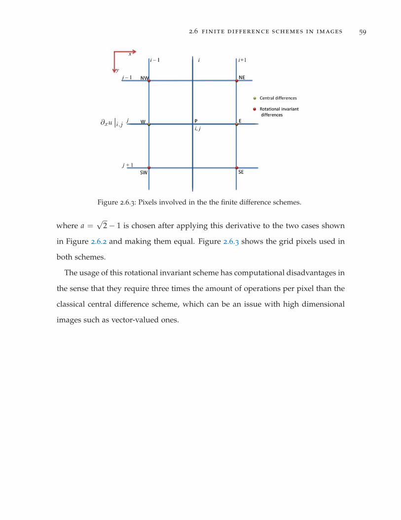
2.6 finite difference schemes in images 59
Figure 2.6.3: Pixels involved in the the finite difference schemes.
where a =√
2 − 1 is chosen after applying this derivative to the two cases shown
in Figure 2.6.2 and making them equal. Figure 2.6.3 shows the grid pixels used in
both schemes.
The usage of this rotational invariant scheme has computational disadvantages in
the sense that they require three times the amount of operations per pixel than the
classical central difference scheme, which can be an issue with high dimensional
images such as vector-valued ones.

3T H E S P E C T R A L LY W E I G H T E D S T R U C T U R E T E N S O R
3.1 structure tensor
An extension of the structure tensor for vector–valued images, such as color im-
ages, was presented by Di Zenzo [67]. His idea was to have one edge descriptor
for all bands, so any process following the edges found by the structure tensor will
behave the same way in each channel and have the information from all channels.
Processing each channel independently has several drawbacks such as edge dislo-
cation and unwanted discontinuities [71]. Di Zenzo’s structure tensor is based on
the idea that edge information along a given direction in one channel must rein-
force edge evidence in the other channels. Hence, all edge information can be fused
by using pixel-based averaging along the spectral values of its initial matrix field.
Di Zenzo’s method assumes that each band provides the same amount of edge
information and gives each band the same weight [67]. This may work well with
RGB images that only have three bands, but in the case of an HSI with hundreds of
bands, edge information may not appear in all bands. Depending on the spectrum
interval being sampled and the object’s materials composition, some bands of an
HSI will show all or parts of its edges and some will not. Therefore, weighting the
spectra depending on the amount of edge information they provide may prove a
more effective extension of the structure tensor to HSI’s than simple averaging.
Structure tensors are classified as linear and nonlinear. Linear structure tensors
are defined formally in Section 3.1.2. Nonlinear structure tensors are usually used
60

3.1 structure tensor 61
in iterative processes where the structure tensor output from iteration n is used as
the input for iteration n + 1. The weighting scheme proposed in this work can be
used with both linear and nonlinear structure tensors that are applied to vector-
valued data. As with all Di Zenzo’s structure tensors, there is a caveat, the range of
the data in each channel has to be similar. If not, it is necessary to rescale the data.
In HSI images, the structure tensor can be weighted in the spatial dimensions or
the spectral dimensions. Spatially weighted structure tensors have been proposed
in [65, 66] mainly to make the structure tensor spatially data-adaptive while a
spectrally weighted structure tensor [79] is used to fuse the scalar structure tensor
information from many bands. The method proposed in this research belongs to
the latter with the added capability to be data–adaptive in the spectral direction.
Structure tensors based on robust statistics are one of the most important spatial
weighting techniques since the structure tensor is nonlinear and the weights are
based on the data. They were proposed by [65] and further developed in [66, 80, 81].
The structure tensors based on nonlinear diffusion, introduced by [21] and [82],
belong to the data-adaptive methods, i.e, methods that try to adapt the structure
tensor to the information in a neighborhood. Structure tensors based on robust
statistical methods avoid the data adaptive processing by estimating the orientation
in a neighborhood using robust error measures.
Spectrally weighted structure tensors have been studied less since much of the
structure tensor work focuses on color images with only three bands. Averag-
ing three bands is simple, computationally inexpensive and produces good results.
There is, however, a spectrally weighted structure tensor for color images proposed
by [79]. In this case, a-priori knowledge of the reliability and noise level in each
channel is required, which limits its use. Recently, a weighted zero mean structure
tensor for vector valued images has been proposed by [83] using weights based on
the median of the data. But it suffers from artifacts if the mean is in the data. In

3.1 structure tensor 62
the following Sections, the classical structure tensor for vector valued images will
be defined and some of the best known variants will be described. The spectrally
weighted structure tensor will be defined. A weighting process will be presented
for the case in which the spectrum of the images are locally highly correlated.
3.1.1 Di Zenzo Structure Tensor
Di Zenzo [67] presented a definition of the gradient that uses concepts from classic
differential geometry, see (2.3.3.3) given by:
J = ∑j∇ f j∇ f T
j
for an image f in a neighborhood of a pixel at p. The edge strength can be defined
as a function g of the maximum and minimum eigenvalues of J. For the case of 2D
images this will be μ1 ≥ μ2. Many functions have been proposed [45, 72, 84]. For
example,
g(μ1, μ2) = μ1 + μ2 =m
∑i|∇ fi|2.
For the scalar case where m = 1, g reduces to |∇ fi|2, which is the measure of edge
strength for scalar images. For the nonlinear case, the solution u is used instead of
f in each iteration n, where for n = 0, u = f . The following tensor is known as Di
Zenzo’s structure tensor
J0 =m
∑j=1
∇uj∇uTj . (3.1.1)

3.1 structure tensor 63
3.1.2 Classical structure tensor
This section will recall some definitions presented in Section 2.3.5 so there is an
easier flow of ideas. The extension of the structure tensor to vector valued images
is done using Di Zenzo’s structure tensor :
J0 =m
∑i=1
∇uσ,i∇uTσ,i. (3.1.2)
where ∇uσ,i is the smoothed gradient of band i defined in (2.1.2). The fusion of
the edge information in each channel is done by averaging Di Zenzo’s structure
tensor along the spectral direction. Following the notation in Section 2.3.5 the
initial matrix field for the vector valued images is obtained by :
J0 =1m
m
∑i=1
J0i =1m
⎡⎢⎢⎢⎣
m
∑i=1
I2x,i
m
∑i=1
Ix,i Iy,i
m
∑i=1
Ix,i Iy,i
m
∑i=1
I2y,i
⎤⎥⎥⎥⎦ (3.1.3)
Then the structure tensor for a neighborhood of scale ρ is computed as:
Jρ = Gρ ∗ J0 =
⎡⎢⎣ Gρ ∗ J011 Gρ ∗ J012
Gρ ∗ J012 Gρ ∗ J022
⎤⎥⎦ =
⎡⎢⎣ a b
b c
⎤⎥⎦ ρ > 0. (3.1.4)
Since Jρ is symmetric positive definite, then it is possible to find an eigen-decomposition
with orthonormal eigenvectors ω1, ω2 given by:
Jρ =
[ω1 ω2
] ⎡⎢⎣ μ1 0
0 μ2
⎤⎥⎦ [ ω1 ω2
]Tρ ≥ 0, (3.1.5)

3.1 structure tensor 64
where
ω1 ‖
⎡⎢⎣ 2b
c − a +√(a − c)2 + 4b2
⎤⎥⎦ and ω2 ‖
⎡⎢⎣ a − c −
√(a − c)2 + 4b2
2b
⎤⎥⎦ (3.1.6)
the symbol ‖ means ‘parallel to’ and the corresponding eigenvalues μ1 and μ2 are
given by
μ1 =a + c +
√(a − c)2 + 4b2
2and μ2 =
a + c −√(a − c)2 + 4b2
2.
Jρ is the average of the gradient orientations in a neighborhood of size O(ρ). Its
eigenvalues measure the average contrast, i.e., the gray value fluctuation for all
bands along the eigen-directions within the integration scale ρ. If μ1 > μ2, then
ω1 is the direction of higher average contrast, and ω2 gives the preferred local
orientation or coherence orientation [20]. The structure tensor defined in (3.1.4) has
two advantages: (i) robustness under noise as a result of smoothing the resulting
matrix field, and (ii) additional information is created by averaging the local orien-
tation. It then becomes possible to distinguish areas where structures are oriented
uniformly like in the regions between edges. This effect allows estimation of the
dominant orientation on those points in the image where the gradient is close to
zero [66]. Its major drawback is that it can lead to inaccurate estimation when
the local neighborhood is not homogeneous like near the boundary between two
different textures or two different moving objects [66], see Section 2.2.2.
3.1.3 Methods to Enhance the Local Orientation
The problem of enhancing the local orientation estimation using the structure ten-
sor has been approached from two perspectives:
3.1 structure tensor 65
1. Adapt the neighborhood to the data (i.e., to the image’s local geometry) or
2. Choose one of the ambiguous orientations keeping the non-adaptive window
[66].
In order to adapt the neighborhood to the data, several methods have been pro-
posed such as those using Kuwahara-Nagao operator [85, 86, 87, 88], adaptive
Gaussian filters [89, 90, 91, 92], and nonlinear diffusion [21, 82]. In the last method,
the structure tensor is part of an iterative process that instead of applying a Gaus-
sian convolution, as in (2.3.14), applies nonlinear diffusion. The Gaussian convolu-
tion is used for the integration step so neighborhoods become data-adaptive. While
Gaussian smoothing is equivalent to diffusion with constant diffusivity, nonlinear
diffusion reduces the amount of smoothing in the presence of discontinuities in the
data, i.e., edges. The discontinuities are determined iteratively in the updated and
smoothed data, and therefore, one can integrate data from an arbitrarily shaped
neighborhood [66].
The other framework uses robust statistics to estimate one of the ambiguous ori-
entations, so it is not necessary to find an adaptive window [65, 66, 80]. Structure
tensors based on robust statistics are motivated by a result from [65] that shows
that least squares estimation procedures for local orientation reduce to solving an
eigenvalue problem for the initial matrix field smoothed by a Gaussian kernel , i.e.,
the structure tensor, see Section 2.3.3.1. Least squares estimation procedures use a
quadratic error measure which is very sensitive to outliers. In [65], the quadratic er-
ror measure is changed for a more robust one which imposes smaller penalties on
outliers to reduce their influence in the error measure. Robust error measures like
Gaussian robust error [65] or Geman-McClure [80] ‘clamp’ the influence of large
outliers to a maximum of one. Then an iterative approach is required to solve for
a robust structure-tensor matrix as it becomes non-linearly dependent on the local
orientation of the neighborhood.

3.2 the spectrally weighted structure tensor 66
The next section will present a general definition of the weighted structure tensor.
Section 3.2.1 describes weights based on the median.
3.2 the spectrally weighted structure tensor
The initial matrix field in Equation (3.1.4) describes the fusion step in the classical
structure tensor. The proposed method modifies this step. Instead of using the
uniform distribution and assigning the same weight to each band, a weighted initial
matrix field in each channel will be defined as the scalar tensor product:
Jok = [Wk ◦ ∇uσ,k] [Wk ◦ ∇uσ,k]T
where Wk = [wx,k, wy,k]T are the weights for band k. The initial matrix field for the
vector-valued case with weights wx, wy, and wxy = wxwy is calculated as
J0 =m
∑k=1
J0k =
⎡⎢⎢⎢⎣
m
∑k=1
w2x,k ◦ u2
x,i
m
∑k=1
w2xy,k ◦ ux,iuy,i
m
∑k=1
w2xy,k ◦ ux,iuy,i
m
∑k=1
w2y,k ◦ u2
y,i
⎤⎥⎥⎥⎦ =
⎡⎢⎣ A B
B C
⎤⎥⎦ , (3.2.1)
The structure tensor, Jρ will be calculated as in (3.1.4). Jρ for ρ ≥ 0 is still a
tensor as it is a symmetric, positive semi-definite matrix therefore it has the same
eigen-decomposition as in (2.3.15).
3.2.1 Weights Based on the Median.
The weights presented in this section are taken from [83]. This was the first try to
make the structure tensor adaptive in the spectral dimension. These weights are
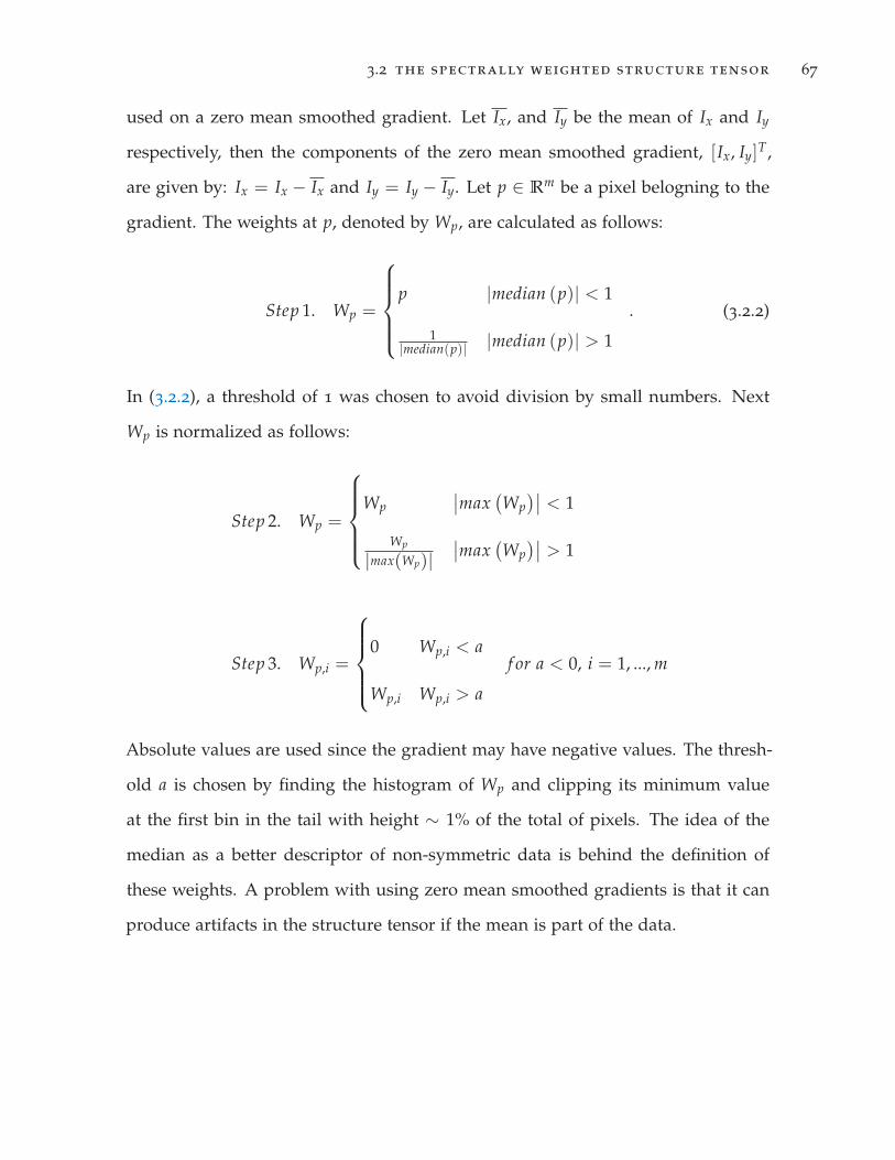
3.2 the spectrally weighted structure tensor 67
used on a zero mean smoothed gradient. Let Ix, and Iy be the mean of Ix and Iy
respectively, then the components of the zero mean smoothed gradient, [Ix, Iy]T,
are given by: Ix = Ix − Ix and Iy = Iy − Iy. Let p ∈ Rm be a pixel belogning to the
gradient. The weights at p, denoted by Wp, are calculated as follows:
Step 1. Wp =
⎧⎪⎪⎪⎨⎪⎪⎪⎩
p |median (p)| < 1
1|median(p)| |median (p)| > 1
. (3.2.2)
In (3.2.2), a threshold of 1 was chosen to avoid division by small numbers. Next
Wp is normalized as follows:
Step 2. Wp =
⎧⎪⎪⎪⎨⎪⎪⎪⎩
Wp∣∣max
(Wp)∣∣ < 1
Wp
|max(Wp)|∣∣max
(Wp)∣∣ > 1
Step 3. Wp,i =
⎧⎪⎪⎪⎨⎪⎪⎪⎩
0 Wp,i < a
Wp,i Wp,i > a
f or a < 0, i = 1, ..., m
Absolute values are used since the gradient may have negative values. The thresh-
old a is chosen by finding the histogram of Wp and clipping its minimum value
at the first bin in the tail with height ∼ 1% of the total of pixels. The idea of the
median as a better descriptor of non-symmetric data is behind the definition of
these weights. A problem with using zero mean smoothed gradients is that it can
produce artifacts in the structure tensor if the mean is part of the data.

3.3 spectrally weighted structure tensor based on the heat operator 68
3.3 spectrally weighted structure tensor based on the heat oper-
ator
In this section, the adaptive spectrally weighted structure tensor is presented. The
classical structure tensor is adaptive to the spatial features in the image. The adap-
tivity of the structure tensor presented here is in the spectral dimension. This is
done by defining weights for each channel of the initial matrix field. The weights
will be defined using the heat operator.
3.3.1 Motivation
Figure 3.3.1 is used to motivate the proposed spectral weights. It presents scatter
plots among several bands of the Indian Pines image (see Section 5.1.1). It also
shows that the same correlation holds among the bands of the gradient component
Ix. The first row shows gray level images of bands 15, 50, 51, 60, and 110 corre-
sponding to 567.38 nm, 879.53 nm, 889.14 nm, 985.27 nm and 1541.59 nm. Band 45,
centered at 831.41 nm, is not shown but looks very similar to band 50. For visualiza-
tion purposes, all images have been contrast stretched so that the minimum value
in the band is black, and the maximum value is white. Note that Figures 3.3.1 (b),
(c) and (d) are visually similar. Note that the edges inside the red square do not
appear in all bands. The second row of Figure 3.3.1 from left to right shows scatter
plots between band 50 and (a) band 15, (b) band 45, (c) band 51, (d) band 60, (e)
band 110. The same range [0, 255] is used for the x-axis and y-axis in all scatter
plots. As expected, the scatter plots showing the highest correlation are (b), (c) and
(d) which correspond to the bands closer to band 50. The scatter plots with bands
farther away from band 50 may not show such a correlation as shown in Figures
3.3.1 (a) and (e). The third row of Figure 3.3.1 shows Ix’s for the bands in the first

3.3 spectrally weighted structure tensor based on the heat operator 69
Figure 3.3.1: Bands of the same HSI compared to the respective bands of its gradient com-ponent Ix. FIRST ROW (left to right): Indian Pines’ bands (a) 15, (b) 50, (c) 51,(d) 60, (e) 110. SECOND ROW: Scatter plots between Indian Pines’ band 50and (left to right) (a) band 15, (b) band 45, (c) band 51, (d) band 60 (e) band110. THIRD ROW (left to right): Ix’s bands (a) 15, (b) 50, (c) 51, (d) 60, (e) 110.FOURTH ROW: Scatter plots between gradient component Ix’s band 50 and(left to right) (a) bands 15,( b) band 45, (c) band 51, (d) band 60 (e) band 110.

3.3 spectrally weighted structure tensor based on the heat operator 70
row of Figure 3.3.1. Visual inspection shows that in the third row band 50 in (b) is
very similar to band 51 in (c) and band 60 in (d). The fourth row shows the scatter
plots for Ix that correspond to the same bands as the second row. The axes of the
scatter plot are equal and set to [ai, bi], where ai = min[min(band 50), min(band i)]
for i = 15, 45, 51, 60, 110 and bi is defined the same using max instead of min.
As with the original image, there is a linear correlation between nearby bands and
that relation does not hold for bands that are farther away. Similar results can be
obtained using Iy (not shown).
Figure 3.3.1 shows that even though ∇Iσ does not provide direct information
on the change of the intensity along the spectral dimension, it preserves the cor-
relation between bands. This result is not surprising since spatial derivatives are
implemented as derivatives of a Gaussian which are transformations that preserve
correlation. The fusion step must weight these local correlations by taking the val-
ues of the neighbor spectra into account. So, pixels with similar responses will have
similar weights and preserve the differences with other non-similar pixels. An op-
erator that preserves these kinds of local relationships is the heat operator [93]. To
use the heat operator, the smoothed gradient is modeled as the initial heat distri-
bution on a compact manifold M in which each point x in M is an m−dimensional
vector.
The next section will present a short overview of the mathematical background
for the heat operator and Section 3.3.3 presents the proposed weights.
3.3.2 The Heat Operator
The heat operator is used as part of the heat kernel which in turn is used as part
of a structure preserving map that finds intrinsic symmetries between shapes [94].
Here it is used as the operator that acts on the spectral signature of each pixel

3.3 spectrally weighted structure tensor based on the heat operator 71
of the gradient components producing the weights. This section presents a brief
introduction to it.
Let M be a compact Riemannian manifold without boundary. Let Rm+ be the
positive section of the m−dimensional Euclidean space, Rm. Let the amount of
heat at a point p ∈ M at time s for some initial heat distribution f : M → Rm+ at
s = 0 be defined as h(p, s) : M × R+ → Rm+, where h (p, s) is a solution to the heat
equation
∂sh = −ΔMh, and lims→0
h (p, s) = f (p) ,
and ΔMis the Laplace-Beltrami operator of M, for an introduction of this operator
see [95]. The solution of the heat equation at time s given f , can be computed
through the heat operator Hs : L2 → L2, where L2 is the space of all smooth, square
integrable functions on M:
h (p, s) = (Hs f ) (p) =(
e−sΔM f)(p) (3.3.1)
These results can be found in [93]. Information about properties and applications
of (3.3.1) can be found in [93, 96, 94].
3.3.3 Weights Based on the Heat Operator
This section presents the proposed weighting process applied to the classical struc-
ture tensor. From Section 3.3.2, M can be thought of as an abstract space general-
ization that locally behaves as the Euclidean space and where ∇Iσ resides. Let p

3.3 spectrally weighted structure tensor based on the heat operator 72
be a pixel on the smoothed original image Iσ. The weights are given by h(p, s) in
(3.3.1) with initial heat distribution
f (p) = ∇I∗σ (p) =
⎡⎢⎣ I∗x (p)
I∗y (p)
⎤⎥⎦
where I∗x (p) is Ix (p) after a convolution with a [1× 3] mean filter used to regularize
the weighting process. I∗y (p) is obtained in the same manner. The weights at p
denoted as Wp will be called heat weights. Their definition is based on Hs in (3.3.1),
but the absolute value of the Laplace-Beltrami operator is used to capture the size
of variations independent of their sign. Wp is given as:
Wp =
⎡⎢⎣ wpx
wpy
⎤⎥⎦ =
⎡⎢⎣ e−s|ΔI∗x(p)|
e−s|ΔI∗y(p)|
⎤⎥⎦ . (3.3.2)
Since I∗x (p) is an m−dimensional vector, its Laplace-Beltrami operator is its second
derivative. The same is true for I∗y (p). wpx, wpy ∈ Rm are normalized by their
respective sums so that sum(Wp) = [1, 1]T. In all experiments, s = 1 was used.
Higher values of s can dominate Wp’s behavior, corrupting the information pro-
duced by the Laplace-Beltrami operator (see Section 5.3.). This weighting process
takes into account the correlation between bands in two ways: (i) using the mean
filter and (ii) approximating the Laplace-Beltrami operator using the standard cen-
tral difference scheme. The spectrally weighted structure tensor with weights based
on the heat operator will be called the heat weighted structure tensor.
Figure 3.3.2 shows how the weights affect the spectral signatures of the gradient
component Ix and how the relations between pixels of the same class are preserved
in a HSI. There are two scenarios depicted in Figure 3.3.2 both with pixels in the
same class, as shown in (b) and (f). The first scenario, depicted in the left column,

3.3 spectrally weighted structure tensor based on the heat operator 73
Figure 3.3.2: Weighting effect in pixels on heterogeneous and homogeneous regions of In-dian Pines. TOP ROW left to right: (a) Portion of Indian Pines image with apixel on an edge and a second pixel on an homogeneous region. (b) Spectra ofthe pixels marked in (a). (c) Ix’s signature of the pixels marked in (a) using theuniform weights (d) Ix’s initial signature of the pixels marked in (a) using theheat weights. BOTTOM ROW left to right: (e) Portion of Indian Pines imagewith both pixels in a homogeneous region. (f) Spectra of the pixels marked in(e). (g) Ix’s signature of the pixels marked in (e) using the uniform weights (h)Ix’s signature of the pixels marked in (e) using the heat weights.
3.3 spectrally weighted structure tensor based on the heat operator 74
is the comparison of an edge pixel (red) and a pixel from the inside region (blue).
The second scenario, shown in the right column, compares two pixels inside region.
Figure 3(c) and (d) show Ix’s signature from pixels in the same spatial position as
in (a). As in (b), the signature of the edge pixel is plotted in red and the non-edge
in blue. It can be seen in (c) and (d) that the two signatures are very different as
not all spatial neighbors of the edge pixel belong to the same class. In addition, the
signature of the edge pixel tends to zero along the spectra. This is expected since
it is a horizontal edge and the signature belongs to its horizontal derivative Ix. On
the other hand, when the two pixels are on the inside region, their signatures are
highly similar, as shown in Figures 3.3.2 (f)–(h). Figures 3.3.2 (c) and (g) show the
signature of the pixels on Ix using the uniform weights on both scenarios. Figures
3.3.2 (d) and (h) show the signatures of pixels on Ix using the heat weights. For
this example, a comparison of the angle between the signatures produced with the
uniform weights, θu, and the angle between the signatures produced with the heat
weights, θh, is done using the relative difference measure given by:
% Dif =|θh − θu|
max (|θh| , |θu|) × 100.
In the first case, Figures 3.3.2 (c) and (d), θh in (d) is 0.47% larger than θu in (c).
In the second case, Figures 3.3.2 (g) and (h), θh in (h) is 4.15% smaller than θu in
(g). These results suggest that the heat weights, not only produce smoothing, but
they also reduce the variability between similar signatures, while maintaining the
difference between dissimilar pixels.
From Figure 3.3.2 it is clear that the proposed weighting process produce a
smoothing in the spectral response of each pixel of the spatial gradient images.
Intuitively the heat operator penalize large abrupt changes in the spectral response
of the pixel. In the case of a pixel p = [p1, ..., pm] on I∗x , the x−component of the

3.3 spectrally weighted structure tensor based on the heat operator 75
spatial gradient, the entry pi for band i identify the existence or nonexistence of
vertical spatial edges in that band. The heat operator applied to p will penalize
large changes in the rate of change of the existence of the spatial edges along the
bands at pixel p.
3.3.4 Parameters used for the Structure Tensor.
Two parameters for the structure tensor, Jρ, with ρ > 0 were defined in Section
2.3.5. One is known as the noise scale σ, since the smoothed gradient ∇Iσ ,which is
an edge detector, ignores details smaller than O(σ) [20]. The parameter σ is image
dependent, but our experience with several HSIs is that a value of σ ∈ [0.5, 1.5]
is enough to regularize the process. For degraded images, larger values of σ are
needed [46]. Figure 3.3.3(a) shows the red band of Van Gogh’s painting “Road
with Cypress and Star” [97]. Figures 3.3.3(b) and (c) are the original image after
being processed with TAND-CED (see Section 4.2.2) using the classical structure
tensor. To show the impact of the integration scale ρ parameter, all values are
kept equal except ρ. When ρ = 1 in Figure 3.3.3(b), the filter produces artifacts,
while increasing it to ρ = 4 in Figure 3.3.3(c) produces flow-like structures that
look like completed lines since this larger neighborhood captures the coherence
orientation. Increasing it to ρ = 6, see Figure 3.3.3(d), produces very similar results
to ρ = 4. It is important to note that underestimation of ρ is far more critical than
overestimation, so it is not difficult to find an estimate that works for the whole
image domain [46].

3.3 spectrally weighted structure tensor based on the heat operator 76
Figure 3.3.3: Integration scale on CED. �� = 0.5, n = 4. Image size is 254 × 200. (a) originalimage. (b) After CED with ρ = 1. (c) After CED with ρ = 4. (d) After CEDwith ρ = 6.

3.4 implementation details 77
3.4 implementation details
The Gaussian derivatives for an n1 × n2 ×m image I are implemented by truncating
the uni-variate Gaussian distribution with variance σ2 when the smallest values is
less than 1 × 10⁻⁴. This produces a kernel Gσ. Then the derivatives Ix, Iy are
implemented using separable kernels. Note that Ix and Iy are of the same size as I.
The weights are implemented by converting Ix and Iy to matrices in which each
row is a pixel. Each of those matrices are convolved with the 1 × 3 median fil-
ter and with the second derivative calculated using symmetric central differences.
Then (3.3.2) is calculated and converted back to a cube, producing Wx and Wy. The
weighted derivatives are calculated by Hadamard multiplications (Wx ◦ Ix) and(Wy ◦ Iy
),
denoted by the small circle (◦).Since the derivative is calculated using local neighborhoods all the products used
to calculate the components
A =m
∑i[(Wx ◦ Ix) ◦ (Wx ◦ Ix)]i , B =
m
∑i(Wx ◦ Ix)i ◦
(Wy ◦ Iy
)i and
C =m
∑i
(Wy ◦ Iy
)i ◦(Wy ◦ Iy
)i
of the initial matrix field are Hadamard too. Each of those components produce a
n1 × n2 image with the edge information. Vertical edges are found using A. Diag-
onal edges are found using B and horizontal edges using C. Those A, B and C are
used for EED. A, B and C are convolved with Gρ a Gaussian of variance ρ to calcu-
late the integration step needed for CED’s structure tensor. Gρ is truncated in the
same way as Gσ. It is important to note that all the operations needed to implement
the structure tensor are pixel-wise, so a parallel implementation is possible. Figure
3.4.1 shows a flow chart of the steps need it to calculate the structure tensor. The

3.4 implementation details 78
pseudo-code to implement the proposed weighted structure tensor is described in
3.1.
Algorithm 3.1 Weighted Structure TensorInputs : I, σ, ρOutput: A, B, C
1. Calculate the Gaussian Kernel
• thr ← 0.0001; t ← 1 : 30
• width := f ind(exp(−(t.2)/2σ2) > thr; x ← −width : width
• Gσ ← exp(−(x ◦ x)/2σ2)
• Gσ ← Gσ/sum(Gσ)
2. Calculate Ix, Iy
• Ix ← (I ∗ (−x ◦ Gσ)) ∗ GTσ
• Iy ←(
I ∗ (−x ◦ Gσ)T)∗ Gσ
3. Calculate (Wx ◦ Ix) and(Wy ◦ Iy
)using (3.3.2).
4. Calculate A = ∑mi [(Wx ◦ Ix) ◦ (Wx ◦ Ix)]i
5. Calculate B = ∑mi (Wx ◦ Ix)i ◦
(Wy ◦ Iy
)i
6. Calculate C = ∑mi[(
Wy ◦ Iy) ◦ (Wy ◦ Iy
)]i
7. if ρ �= 0 % for CED
8. A ← A ∗ Gρ
9. B ← B ∗ Gρ
10. C ← C ∗ Gρ
11. endIf

3.4 implementation details 79
Figure 3.4.1: Flow chart describing the proposed Structure Tensor.

3.5 concluding remarks 80
3.5 concluding remarks
In this chapter a framework for the spectrally adapted structure tensor for vector-
valued images has been presented. This framework consist in a weighting process
that takes into account the spectral characteristics of those images. A spectrally
adapted structure tensor for the case in which the spectrum of the vector-valued
images is locally highly correlated have been developed. HSI are an example of
those images. The heat operator give the mathematical framework to use the spec-
tral characteristics of the images for the weighting process.
4T E N S O R A N I S O T R O P I C N O N L I N E A R D I F F U S I O N
This chapter will describe the proposed TAND diffusion tensors. Those tensors are
build based on the structure tensor defined in Section 2.5.3. Extending TAND to
vector-valued images that are locally highly correlated in the spectral direction is
the main motivation to propose them. The diffusion tensors used in the proposed
TAND filters will use the eigenvectors of the spectrally adaptive structure tensor
proposed in the previous chapter. The eigenvalues will be defined so TAND will
take advantage of the edge information obtained by the heat weighted structure
tensor. Experimental results on the usage of the heat weighted structure tensor on
TAND and comparison of the proposed TAND with the state of the art proposed
by Weickert will be presented.
4.1 introduction
TAND is described by the partial differential equation (PDE):
∂u∂t
−∇ · (D∇u) = 0, in Ω (4.1.1)
where u (the filtered version of image f (x) with domain �) is the solution of the
initial boundary value problem for the diffusion equation with f as the initial con-
81

4.2 eigenvalues of the proposed diffusion tensors 82
dition, and Neumann boundary conditions. D is a positive semi definite symmetric
matrix known as the diffusion tensor D is defined as:
D =
[ω1 ω2
] ⎡⎢⎣ κ1 0
0 κ2
⎤⎥⎦⎡⎢⎣ ω1
ω2
⎤⎥⎦ =
⎡⎢⎣ λ β
β ν
⎤⎥⎦ (4.1.2)
where, ω1 = [ω11, ω12 ]T ⊥ ω2 = [−ω12, ω11 ]
T are defined as in (3.1.5). κ1 and κ2
are functions on the largest and smallest eigenvalues of J�, μ1 and μ2 respectively.
λ, β and ν can be written in terms of the eigenvalues and eigenvectors of D as
follows:
λ =κ1ω211+ κ2ω2
12(4.1.3)
β = (κ1 − κ2)ω11ω12 (4.1.4)
ν =κ1ω212+ κ2ω2
11, (4.1.5)
when, ρ = 0, (3.1.3) is the structure tensor used for EED and when � > 0, (3.1.4)
is the structure tensor used for CED. J0 defined in (3.1.3) is used for the classical
structure tensor while J0 defined in (3.2.1) is used for the spectrally weighted tensor.
The next section will present the functions used to define the eigenvalues κ1 and κ2
of D for the proposed TAND.
4.2 eigenvalues of the proposed diffusion tensors
This section will give some motivation to define new diffusion tensors for TAND-
EED and TAND-CED that take advantage of the information produced by the heat
weighted structure tensor. A discussion on why the eigenvalues where defined
using those functions is provided.

4.2 eigenvalues of the proposed diffusion tensors 83
4.2.1 EED diffusion tensor
For EED, the diffusion is directed along the edges, avoiding diffusion across them
and on them. So, both κ1 and κ2 must get close to zero in the presence of an edge
and be maximal in homogeneous regions. There are several functions proposed in
the literature used for the eigenvalues κ1 and κ2. A review of them can be found in
[45]. The proposed κ1 and κ2 are given by :
κ1 =
⎧⎪⎪⎪⎨⎪⎪⎪⎩
1 μ1 = 0
1 − exp(
−Cr(μ1/ψ)r
)μ1 > 0
(4.2.1)
κ2 =
⎧⎪⎪⎪⎨⎪⎪⎪⎩
1 μ1 ≤ ψ
1ξ(κ1
1)4+1
μ1 > ψ
(4.2.2)
κ1 is defined as the one proposed for EED by Weickert in [45] with r = 4, Cr = 3.315
(see [2] §5.1), where 1 = exp(–Cr)(1+ 2Cr · r) and ψ is a contrast parameter. For the
edges (μ1 > ψ), κ2 is a constant defined in terms of the entropy of κ1 at iteration
n = 1, ξ(κ1
1)
and 1 otherwise. κ11 is κ1 calculated using the original image. The
entropy ξ (κ1) is defined as in [98]:
ξ = −255
∑i=1
qi log (qi)
where qi is the probability of that a pixel, belonging to κ1, has intensity i and
qi log (qi) = 0 if qi = 0, . In practice, qi is the histogram count of the ith bin of
κ1’s global intensity histogram. Weickert’s in [45] uses κ2 equal to 1. The problem
of letting κ2 = 1 is that it does not adapt to the structures in the image. The

4.2 eigenvalues of the proposed diffusion tensors 84
Figure 4.2.1: Comparison of the classical structure tensor using κ2 = 1 and κ2 defined asin (4.2.2). (a) RGB composition of HSI Indian Pines after EED using clas-sical structure tensor with κ2 = 1, n = 4 iterations; (b) same as (a) withκ2 = 1/
[ξ(κ1
1
)4+ 1]
, n = 4 for edges, otherwise 1; (c) λ−component of thediffusion tensor in (a); (d) λ−component of the diffusion tensor in (b).
4.2 eigenvalues of the proposed diffusion tensors 85
same smoothing is applied in the direction of ω2 independently of the structures
present in the image. κ2 = 1 produces a strong smoothing in the edges as seen
in Figure 4.2.1(a). The value of κ2 in (4.2.2) will decrease in the presence of an
edge (μ1 > ψ), in which case κ1 ≈ 0 and κ2 ≈ 1/[ξ(κ1
1)4
+ 1]
. κ2 is maximal
in the interior of a region (μ1 ≤ ψ), in which case κ1 ≈ 1 and κ2 ≈ 1. This
definition mitigates the blurring effect in the edges, while keeping the smoothing
in the homogeneous regions as seen in Figure 4.2.1(b). Figure 4.2.1(c) shows the
λ−component of the diffusion tensor based on the classical structure tensor with
κ2 = 1. Clearly this component only preserves the vertical edges (dark edges
representing intensity values close to zero). There is a strong smoothing in all the
other edges (light gray edges). While, in Figure 4.2.1(d), where κ2 is defined as
in (4.2.2), edges are preserved. κ2 needs to have the same value for all edges to
prevent the same edge from having strong smoothing in some places and lesser in
others. So, κ2 was chosen to have a dependency on a global characteristic of κ1 that
does not depend directly on the intensity scale. So, the entropy of κ1 was a natural
choice. The entropy is calculated using the original image since the entropy of the
filtered image u decreases at each iteration, i.e., ξ(un+1) ≤ ξ (un) [46]. So, ξ
(κ1
1)
is
constant for all iterations n.
4.2.2 CED Diffusion tensor
When ρ > 0, the structure tensor Jρ is used to enhance one dimensional features in
the image. In this case, the eigenvalue κ1 is equal to a very small constant α used
to guarantee that the diffusion process never stops and to keep the diffusion tensor
uniformly positive definite [46]. κ2 will depend on the difference in the eigenvalues
of Jρ, i.e., μ = μ1 − μ2. The eigenvalues are defined as in [20]

4.2 eigenvalues of the proposed diffusion tensors 86
Figure 4.2.2: κ2 using (4.2.3). Components of the diffusion tensor using C = 1 in (4.2.3)after n = 1 iterations.
κ1 =α 0 < α � 1
κ2 =
⎧⎪⎪⎪⎨⎪⎪⎪⎩
α μ = 0
α + (1 − α) exp(−Cμ2
)otherwise
(4.2.3)
C = 1 is used. This constant assignment does not work well. Figure 4.2.2 shows
the λ, β, and ν components of the diffusion tensor (see (4.1.2)) using κ2 as defined
in (4.2.3) with C = 1 of an AVIRIS image [99]. In this image, only part of the center
wake is enhanced. The idea of using TAND-CED in this image is to enhance the
wakes by eliminating the radial texture traversing them. If we let C be a variable
then C works as a contrast parameter of μ2 and not of μ as shown in Figure 4.2.4(b).
This can presents problems for images where the majority of the edges responses
in μ are less than one. So it will be better to define κ2 in term of the edges responses
of μ and not on μ2.

4.2 eigenvalues of the proposed diffusion tensors 87
Figure 4.2.3: Comparing κ2 using (4.2.3) and using (4.2.4). (a) Plot of κ2 in (4.2.4), varyingthe value of ψ. (b) Plot of κ2 in (4.2.3), varying the value of C.
The eigenvalues of the diffusion tensor can also be defined using the following
expression [100] with ψ as in (4.2.1):
κ1 =α 0 < α � 1
κ2 =
⎧⎪⎪⎪⎨⎪⎪⎪⎩
α μ = 0
α + (1 − α) exp(
−3.315(μ/ψ)4
)otherwise.
(4.2.4)
The value of the contrast parameter ψ in (4.2.4) defines low contrast regions as
regions where μ < ψ making κ2 ≈ α, and high contrast regions where μ > ψ
making κ2 ≈ 1 as shown in Figure 4.2.3(a). The threshold parameter ψ in (4.2.4) is
a contrast parameter of μ instead of μ2. Figure 4.2.4 shows the AVIRIS image [99],
see Section 5.1.2, processed with heat weighted structure tensor with n = 2, σ = 1.2
ρ = 2.5. That figure shows the components of the diffusion tensor, λ, β, and ν using
(4.2.4) as eigenvalue function for κ2 and its sensibility to changes in the value of
ψ for ψ = 70th, 92th and 98th percentile of μ. It is clear that varying ψ produces
enhancement in different features of the image. If C in (4.2.3) is taken as a contrast
parameter and the majority of the values of μ are greater than 1 then (4.2.3) and
(4.2.4) can produce very similar results. For all CED experiment presented in this

4.3 tand as an approximation to local diffusion 88
Figure 4.2.4: Proposed diffusion tensor for CED and its sensibility to ψ. AVIRIS image [99]was process with heat weighted structure tensor with n = 2, σ = 1.2 ρ = 2.5.Components of the diffusion tensor, λ, β, and ν using (4.2.4) as eigenvaluefunction for κ2 vs. ψ are shown. ψ = 70th, 92th and 98th percentile of μ.
work the eigenvalues of the diffusion tensor will be defined as in (4.2.4), otherwise
will be specified. For CED, the value of the noise scale σ needs to be set small
enough so the orientation information is not destroyed.
4.3 tand as an approximation to local diffusion
One of the most studied diffusion PDE-based methods is TAND [21, 2, 20, 46].
TAND was proposed by Weickert in [71]. This filter belongs to a family of regu-
larized anisotropic nonlinear filters that have many proved properties such as well-
posedness (existence and uniqueness of results), continuous dependence of the so-
lution on the initial image and scale space properties such as maximum–minimum

4.3 tand as an approximation to local diffusion 89
principles, invariance, Lyapunov functionals, and convergence to a constant steady-
state. In addition, a scale space discrete theory has been developed [2].
Tschumperlé and Derriche in [18] found that the divergence operator in TAND
can be decomposed as a trace-base operator on the Hessian, H, plus a term that
appears connected to the spatial variation of the tensor field produced by D, i.e.,
div (D∇Ii) = trace (DHi) +∇ITi−→div (D) i = 1, ...m (4.3.1)
where
−→div (D) =
⎛⎜⎜⎜⎜⎝
div
[(λ β
)T]
div
[(β ν
)T]⎞⎟⎟⎟⎟⎠
and λ, β and ν are the components of D, i = 1, . . . , m. This is because they see D in
(4.1.1) as a global operator (i.e., a tensor field on Ω), and not a local operator at a
neighborhood of a pixel p ∈ Ω as in (4.4.1). So, λ, β and ν are no longer constants
at p, they are now functions from Ω → R. Then, it is concluded in [12] that the
first term in (4.3.1) corresponds to local smoothing directed by the elements of D
and that the second term perturbs the smoothing behavior steered by D in the first
term. In this work, the second term in the right hand side of (4.3.1) will be called
the disturbance term. They express (4.3.1) as a sum of two trace terms. To show
all these calculations, they use the initial matrix in (3.1.3) ([12]§3.2-3.3). For the
general framework ([12]§3.4) based on a generalization of the operator trace(DHi),
they choose to use the structure tensor in (3.1.4).
All the examples presented in this framework [12, 3] were compared with TAND–CED.
This comparison appears to be a natural choice since this method uses an integra-
tion parameter ρ > 0, just as in TAND–CED. However, by observing how the eigen-
values of both methods are selected, it becomes clear that, for their diffusion tensor,
they are selected to do very different processes. Hence, a comparison of the two

4.3 tand as an approximation to local diffusion 90
may not be appropriate. Perhaps a better comparison with Weickert’s TAND–EED.
This is also supported in the derivation of their unifying framework ([12] §3.3) since
they use the initial matrix field there. In addition, TAND–EED is designed with the
same purpose as the trace–based formulation. Both aim to preserve and produce
small enhancement on the edges with strong smoothing of the homogeneous ar-
eas. CED, on the other hand, aims to enhance the edges by completing them with
almost no smoothing of the homogeneous regions. To briefly explain this, both κ1
and κ2, in the trace-based formulation, use the decreasing functions given by [12]:
κ1 =1
1 + (√
μ1 + μ2)2 , κ1 =
1√1 + (
√μ1 + μ2)
2(4.3.2)
In the presence of a homogeneous region, μ1 ≈ μ2 ≈ 0, κ1 ≈ κ2 ≈ 1 produce a
strong smoothing. This is true for κ1 and κ2 in (4.3.2) for the trace based formulation
and also for κ1 in (4.2.1) and κ2 = 1 for Weickert’s TAND–EED. For TAND–CED,
κ1 ≈ κ2 ≈ α = 1 × 10⁻³, produces almost no smoothing. In the case of edges,
μ1 � μ2 ≈ 0, κ1 and κ2 in (4.3.2) vanish to zero. κ2 vanishes slower than κ1 ,
producing a very small enhancement along the edges. κ1 in (4.2.1) for TAND–EED
behaves similarly to κ1 in (4.3.2) and produces a small enhancement for edges
with intensity greater than ψ, and κ2 = 1. In TAND–CED, κ1 is a small constant,
α = 1 × 10⁻³, and κ2 reaches its maximum value of 1 for edges with intensity
greater than ψ. In general, the diffusion tensor for the trace–based operator behaves
more similar to TAND for EED than CED.
Empirically speaking, in the experience with TAND processing of HSIs, the in-
fluence of the second term in the RHS of (4.3.1) is not noticeable in the sense that
TAND will still enhance the features as expected, (see Section 5.5.1.2). Hence, the
experiments performed indicate that the computational cost justifies the orientation
and magnitude inaccuracies introduced by this term, if any is really introduced.

4.3 tand as an approximation to local diffusion 91
However, further study comparing TAND–EED and the trace-based formulation
is needed as well as a study of the properties of this general trace based formula-
tion to see if the properties of TAND are extensible to this more general approach.
Neither are addressed in this thesis.
Computationally speaking, to calculate the trace-based operator, it is necessary
to calculate the gradient and Hessian at each pixel entry. There are two ways to
approximate the Hessian: (i) using a finite difference approach or (ii) using spa-
tially varying normalized Gaussian kernels. The approximation that gives results
comparable with TAND–EED using semi-implicit methods is the one using Gaus-
sian kernels. This approximation has a high computational cost since Gaussian
kernels need to be calculated at each pixel entry and then a local convolution is
performed. But it is accurate and this scheme guarantees that the trace–based for-
mulation preserves the maximum principle. The heat weighted structure tensor
can also be used in the trace-based formulation. TAND was chosen since two kind
of processing can be done with it, regularization and structure enhancement, and
given that HSI are large data sets, a tradeoff between accuracy and computational
cost is also necessary.

4.4 discretization of the divergence-based diffusion equation using a tensor 92
4.4 discretization of the divergence-based diffusion equation us-
ing a tensor
The anisotropic diffusion filter in (4.1.1) can be written as
∂u∂t
=div (D∇u)
∂u∂t
∣∣∣N (p) =div
⎡⎢⎣ λ∂xu + β∂yu
β∂yu + ν∂yu
⎤⎥⎦
=∂x (λ∂xu) + ∂x(
β∂yu)+ ∂y
(β∂yu
)+ ∂y
(ν∂yu
)(4.4.1)
where N (p) is a neighborhood around pixel p. Equation (4.4.1) cannot be solved
analytically. It needs to be approximated by numerical methods. Finite difference
methods are most commonly used, see (Section 2.6). They are easy to implement
and they work well with a regular rectangular pixel grid, such as those present in
digital images (see [101]).
For images, it is customary to assume that the pixel size in the x and y direction
is 1. Let τ be the time step size, and denote Uni,j as the approximation of u at pixel
p = (i, j) at time tn = n�. A simple finite difference approximation to ∂tu at pixel p
for iteration n is given by:
∂tu =Un+1
p − Unp
τ(4.4.2)
To include the neighbors in the 3 × 3 neighborhood and to produce a symmetric
derivative, the spatial derivatives are approximated as follows:
δ∗xUi,j = Uni+ 1
2 ,j − Uni− 1
2 ,j, and δ∗yUi,j = Uni,j+ 1
2− Un
i,j− 12, (4.4.3)

4.4 discretization of the divergence-based diffusion equation using a tensor 93
Figure 4.4.1: Pixels involved in the approximation of the divergence term for the classicaland rotational invariant difference schemes
which corresponds to the green dots in Figure 4.4.1(a). Then, the right hand side
of (4.4.1) is approximated as:
∂x (λn∂xun)
∣∣i,j ≈ (λni,jδ
∗xUn
i,j
)i+ 1
2 ,j−(
λni,jδ
∗xUn
i,j
)i− 1
2 ,j
≈λni+ 1
2 ,j
(Un
i+ 12 ,j − Un
i− 12 ,j
)i+ 1
2 ,j− λn
i− 12 ,j
(Un
i+ 12 ,j − Un
i− 12 ,j
)i− 1
2 ,j
∂x (λn∂xun)
∣∣i,j ≈λnE + λn
P2
(UE − UP) +λn
P + λnW
2(UW − UP) .
In an analogous form it is found that ∂y(ν∂yu
) ∣∣i,j given by:
∂y(νn∂yun) ∣∣i,j ≈ νn
S + νP
2(US − UP) +
νnP + νn
N2
(UN − UP) .
For the mixed derivatives, there are several possibilities:
scheme 1. Using the standard central differences in (2.6.1) :

4.4 discretization of the divergence-based diffusion equation using a tensor 94
Table 4.4.1: 3 × 3 averaging mask A(
Uni,j
)for the case in which the mixed derivatives are
calculated using the standard central differences defined by δx in 2.6.1βN+βW
4νN+νP
2βE+βN
4
λW+λP2 −
⎛⎜⎝
λE+λP2 + λW+λP
2
νN+νP2 + νS+νP
2
⎞⎟⎠ λE+λP
2
βW+βS4
νS+νP2
βE+βS4
∂x(
βn∂yun) ∣∣i,j ≈(
βni,jδyUn
i,j
)i+1,j
−(
βni,jδyUn
i,j
)i−1,j
2
≈βn
i+1,j
4
(Un
i,j+1 − Uni,j−1
)i+1,j
−βn
i−1,j
4
(Un
i,j+1 − Uni,j−1
)i−1,j
≈βn
i+1,j
4Un
i+1,j+1 − Uni+1,j−1 −
βni−1,j
4Un
i−1,j+1 − Uni−1,j−1
≈βnE
4(Un
SE − UnNE) +
βnW4
(UnNW − Un
SW)
In an analogous manner, the other mixed derivative is calculated
∂y (βn∂xu)∣∣i,j ≈ βn
S4
(UnSE − Un
SW) +βn
N4
(UnNW − Un
NE)
The preceding approximations lead to the scheme:
Un+1P − Un
Pτ
=λn
E + λnP
2(UE − UP) +
λnP + λn
W2
(UW − UP)
+νn
S + νnP
2(US − UP) +
νnP + νn
N2
(UN − UP)
+βn
E4
(UnSE − Un
NE) +βn
W4
(UnNW − Un
SW)
+βn
S4
(UnSE − Un
SW) +βn
N4
(UnNW − Un
NE)

4.4 discretization of the divergence-based diffusion equation using a tensor 95
Table 4.4.2: 3 × 3 averaging mask A(
Uni,j
)for the case in which the mixed derivatives are
calculated using the standard central differences defined by δ∗x in (4.4.3).
βW+βN+2βP8
12 (νN + νP) +18 (βW − βE)
βE+βN+2βP8
12 (λW + λP) +
18 (βN − βS)
−(
λE+λW2 + λP
νN+νS2 + νP
)12 (λE + λP) +
18 (βS − βN)
βW+βS+2βP8
12 (νS + νP) +18 (βE − βW)
βE+βS+2βP8
As a result, the unknown Un+1P can be calculated explicitly as a weighted mean of
known values at level n. In stencil notation, the averaging mask is given by Table
4.4.1.
scheme 2. Using the central differences in (4.4.3):
∂x(
βn∂yun) ∣∣i,j ≈ (βni,jδ
∗xUn
i,j
)i+ 1
2 ,j−(
βni,jδ
∗xUn
i,j
)i− 1
2 ,j
≈βni+ 1
2 ,j
(Un
i,j+ 12− Un
i,j− 12
)i+ 1
2 ,j− βn
i− 12 ,j
(Un
i,j+ 12− Un
i,j− 12
)i− 1
2 ,j
≈βnE + βn
P2
(Un
i+ 12 ,j+ 1
2− Un
i+ 12 ,j− 1
2
)− βn
W + βnP
2
(Un
i− 12 ,j+ 1
2− Un
i− 12 ,j− 1
2
)≈βn
E + βnP
8(Un
S + UnSE − Un
N − UnNE)
+βn
W + βnP
8(Un
N + UnNW − Un
S − UnSW)
In an analogous manner, the other mixed derivative is calculated
∂y (βn∂xun)∣∣i,j ≈βn
S + βnP
8(Un
E + UnSE − Un
SW − UnW)
+βn
N + βnP
8(Un
W + UnNW − Un
E − UnNE)
Note that for this scheme, interpolations for β’s and U’s are necessary. To use this
scheme on the mixed derivatives, the values on the green dots in Figure 4.4.1(b)

4.4 discretization of the divergence-based diffusion equation using a tensor 96
need to be interpolated. They are interpolated using all the neighbors of pixel P
and P itself, that is, the red dots in Figure 4.4.1(b). e.g.,
Uni+ 1
2 ,j+ 12=
14
(Un
i,j + Uni+1,j + Un
i+1,j+1 + Uni,j+1
)=
14(Un
P + UnE + Un
SE + UnS)
For this scheme the averaging mask is given in Table 4.4.2.
scheme 3. Using the rotationally invariant scheme (2.6.2):
The inclusion of NW, SW, NE, SE neighbors of pixel P produces a grid shown in
Figure 4.4.1(b). The black dots are additional interpolations needed to calculate the
rotationally invariant scheme. The coefficients for the rotationally invariant scheme
were calculated using Matlab’s symbolic package. The expressions are too long to
be displayed here.
It was found, that Schemes 1 and 2 produced similar results. Scheme 3 that
includes the eight neighbors produced less blurry diagonal edges. But as TAND
iterates, some other important edges where smoothed, while the other schemes did
not produce such results. Therefore, due to less computational complexity, fewer
interpolations and the quality of the results Scheme 1 was chosen, i.e, the mixed
derivatives used the standard central difference scheme.
After solving all the spatial derivatives approximations, (4.4.2) can be expressed
as a product of Unp and an averaging mask, A(Un
p), written as a function of Unp (see
[2]). Equation (4.4.1) in matrix-vector notation becomes:
Un+1 = [Id + τA (Un)]Un,
where Id is the identity matrix. This scheme is known as the explicit scheme. The
problem with this scheme is that it is only experimentally stable for step sizes τ ≤ ¼

4.5 solver and preconditioner used 97
which makes the discretization impractical [2]. There is another discretization of
(4.4.1) that is numerically stable for any size of τ since [Id − τA (Un)] is diagonal
dominant, known as semi implicit,
Un = [Id − τA (Un)]Un+1
The accuracy of the solution depends on the choice of τ. With a large τ, the solution
can be obtained within few iterations but the accuracy will suffer to the point that
is useless. A trade-off between the number of iterations n and τ’s size is necessary.
This semi-implicit finite-difference scheme produces a nine diagonal linear system
that is not symmetric and can be solved with any of the Krylov subspace methods
for non-symmetric sparse matrices[102]. The most used are Generalized Minimum
Residual Method (GMRES) or conjugated gradient stabilized method (BICGStab).
4.5 solver and preconditioner used
The 145× 145× 185 Indian Pines HSI was used in experiments to determine whether
to choose BiCGStab or GMRES. TAND was iterated until n = 8, the methods were
set to stop with a tolerance of 10−3 and the time step for the discretization was
τ = 2. As TAND iterates the number of iterations and time it needs to solve the
linear system was decreasing. The experiments where carried out with the three
discretization schemes described in the last section. BiCGStab without precondi-
tioning was three times faster than GMRES in all of them for the first iteration. For
all the other iterations it was at least 1.5 times faster than GMRES. So BiCGStab
was chosen as the solver. Scheme 3 has the best performance in terms of the time
taken to converge to a solution and with fewer iterations. But the discretization
step took 1.5 times longer than with any of the other schemes. Scheme 1 and 2 had

4.6 tand algorithm 98
similar performance, being Scheme 1 slightly better than Scheme 2. So Scheme 1
was chosen.
A preconditioner based on Peric’s direct method to solve nine - diagonal linear
systems [103] was developed. The details of this preconditioner are in Appendix
A.2. This preconditioner was compared with the ILU(0) preconditioner and the
Jacobi explicit diagonalization scheme. ILU was almost 2.8 times faster than Jacobi
diagonalization and 2.25 times faster than our proposed preconditioner. Those
times were calculated in the first iteration of TAND.
4.6 tand algorithm
TAND algorithm is depicted using a flow chart in Figure 4.6.1, its pseudo-code is
given by Algorithm 4.1.
4.7 concluding remarks
A Tensor Anisotropic Nonlinear Diffusion (TAND) have been proposed and stud-
ied. Diffusion tensors were proposed for TAND for Edge Enhancement Diffusion
(EED) and for Coherence Enhancement Diffusion (CED). Those proposed diffu-
sion tensors used the orientation and eigenvalues of heat weighted structure tensor
developed in Chapter 3. This structure tensor make TAND adaptive to the spec-
tral characteristics of HSI. The proposed diffusion tensor for TAND-CED is more
sensitive to the values of the contrast parameter used to define the edges, while
Weickert’s one is sensitive to its square.
All aspects of TAND implementation have been studied. After implementing
three methods to discretize the derivatives, the standard central difference scheme
used to discretize the mixed derivatives ∂xy, ∂yx, and the standard central differ-

4.7 concluding remarks 99
Figure 4.6.1: Flow chart of the TAND algorithm

4.7 concluding remarks 100
Algorithm 4.1 Tensor Anisotropic Nonlinear DiffusionINPUT:
Image Un
Information from Un’s structure tensor to be used.
• Eignvectors of structure tensor ωn1 ωn
2 .
• For EED: The largest eigenvalue, μn1 .
• For CED The difference between the eigenvalues, μ = μn1 − μn
2 .
Contrast parameter ψ
OUTPUT: Image Un+1
1. Calculate κ1, κ2
• For EED use (4.2.1) and (4.2.2)
• For CED use (4.2.4)
2. Calculate the components of the diffusion tensor λn, βn, νn using (4.1.3),(4.1.4) and (4.1.5) respectively
3. Construct the averaging mask A using λ, β, ν. %See the section above
4. Apply boundary conditions
5. Solve the linear system AUn+1 = B

4.7 concluding remarks 101
ence scheme applied to half distances to discretize ∂2x and ∂2
y obtained good results
in term of interpolations, less computational time and good results. To solve the lin-
ear system it was studied the performance of two methods to solve non-symmetric
linear systems, BiCGStab and GMRES. BiCGStab was chosen since it needed less
iterations and less time to find a solution. A preconditioner was developed and
tested against the ILU(0) and the Jacobi explicit diagonalization preconditioner.
The ILU(0) was choosen since it needed less iterations and less time to find the
solution.

5E X P E R I M E N TA L R E S U LT S
This chapter presents the data used for the experiments, and an empirical guideline
to set the parameters used in TAND. Comparison between Nonlinear diffusion
and TAND is performed to see the importance of using a tensor. An experimental
comparison of the performance of the structure tensors using TAND is presented.
To that end, the proposed TAND for EED and CED are used and the comparison
is performed by only changing the structure tensor. The aim of these experiments
is to show how a weighted structure tensor improves the proposed TAND. Finally
a comparison of Weickert’s TAND with the proposed TAND is presented.
All methods were implemented in Matlab. The heat weighted structure tensor
was implemented as described in Algorithm 3.1. The classical structure tensor was
implemented as described in Subsection 3.1. TAND was implemented as described
in Algorithm 4.1. All HSIs bands were normalized to the [0, 255] range (8-bits).
The diffusion tensor for TAND–CED is defined using (4.2.4) and for TAND–EED
using (4.2.1) and (4.2.2). They will show comparisons with the classical structure
tensor. In all experiments, a semi-implicit scheme was used, which is solved using
BICGStab with a tolerance of 10−4 and the discretization time step was τ = 5, any
change on those parameters will be specified. For some images, those methods
were slow to converge. So, to accelerate the convergence the ILU(0) preconditioner
was used.
102

5.1 data 103
5.1 data
5.1.1 Data for EED
For EED, the following HSI were used:
1. The Indian Pines image taken with the AVIRIS (Airborne Visible/Infrared
Imaging Spectrometer) sensor, flown by NASA/Ames on June 12, 1992 over
an area 6 miles west of West Lafayette, IN. This image contains 145 × 145 pix-
els at ∼ 20 m of spatial resolution and 220 spectral bands in the 400− 2500 nm
range, at ∼ 10 nm of spectral resolution, for which ground truth exists. Fifteen
bands were discarded following [5]. Therefore only 185 spectral bands of the
Indian Pines image were used in this work. A false color composite is shown
in Figure 5.1.1(a). Figure 5.1.1(b) shows its ground reference image[105]
2. A 120 × 120 × 145 region of interest (ROI) of the Forest Radiance I was col-
lected by the airborne imaging spectrometer HYDICE over a forest region at
the U.S. Army Aberdeen Proving Ground in 1995 by the HYMSMO (Hyper-
spectral MASINT Support to Military Operations) program. This ROI uses
145 of 224 spectral bands in the 400 − 2500 nm range. The sensor altitude was
5146.33 f t. Bands with low signal to noise ratio were rejected as in [106]. This
region of interest was used since targets are small and discriminating targets
edges are difficult because the image has a strong vertical texture. Ground
truth about target location and signatures is available. A false color composite
of this ROI is shown in Figure 5.1.1(d) with its ground reference image map
shown in Figure 5.1.1(e).
3. The A. P. Hill image captured over Fort. A. P. Hill, Virginia in September
2001 using AVIRIS sensor with ∼ 3.5 m spatial resolution, and 224 spectral

5.1 data 104
Figure 5.1.1: Hyperspectral images used for EED and their classification maps.(a) Falsecolor composite of AVIRIS Indian Pines image with bands [50, 25, 17].(b) Ground reference map for the Indian Pines image (c) True color com-posite of AISA Eagle Guanica dry forest 800 × 800 × 128 with bands[54, 35, 15].(d) False color composite of HYDICE Forest Radiance imagewith bands [75, 37, 18]. (e) Ground reference map for the Forest Radi-ance image (f) False color composite of AVIRIS A. P. Hill image with bands[45, 24, 12]. (g) Classification map for the Composite of Cuprite image withbands [183, 119, 207]. (e)

5.1 data 105
Figure 5.1.2: Cuprite image and its (a) RGB composition of AVIRIS Cuprite image withbands [183, 193, 207] (b) Ground reference map of a ROI of (a) [104].

5.1 data 106
bands in the 400 − 2500 nm range at ∼ 10 nm of spectral resolution. A false
color composite of a 512 × 540 × 224 ROI of this image is shown in Figure
5.1.1(f) and a classification map obtained by minimum distance classifier [107]
is shown in Figure 5.1.1(g)
4. The Cuprite image taken over the mining district, 2 km north of Cuprite,
Nevada, with the AVIRIS sensor, flown by NASA/Ames on June 19, 1997.
This image contains five scenes for a total of 640 × 2378 pixels and 224 bands
in the 370 − 2500 nm range. A ROI of the fourth scene of size 512 × 614 ×224 pixels was selected, a composite of this ROI is shown in Figure 5.1.2(a).
A ground reference map created using the Tetracorder from USGS [104] is
shown in Figure 5.1.2(b).
5. Guanica dry forest images taken in the Southwestern Puerto Rico captured
with the AISA Eagle sensor. Figure 5.1.1(c) presents a true color composite of
a 800× 800× 128 ROI of a registered image composed by three pieces of flight
lines of AISA image. The registration was done using ENVI software. This
image was captured on December of 2007 with a spatial resolution of 1 meter
and 128 spectral bands from 397 nm to 995 nm with a spectral resolution of ∼4.5 nm. Due to its size, this image will be used to test parameters and calculate
number of iterations of the solver. TAND-EED denoising performance will
not be tested with this image.
5.1.2 Data for CED
In this chapter, CED will be used to extract the chain of thyroid cells from a mi-
croscopy HSI and to extract ship wakes from an airborne HSI. All the images where
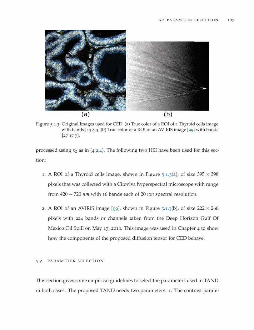
5.2 parameter selection 107
Figure 5.1.3: Original Images used for CED. (a) True color of a ROI of a Thyroid cells imagewith bands [13 8 3].(b) True color of a ROI of an AVIRIS image [99] with bands[27 17 7].
processed using κ2 as in (4.2.4). The following two HSI have been used for this sec-
tion:
1. A ROI of a Thyroid cells image, shown in Figure 5.1.3(a), of size 395 × 398
pixels that was collected with a Citoviva hyperspectral microscope with range
from 420 − 720 nm with 16 bands each of 20 nm spectral resolution.
2. A ROI of an AVIRIS image [99], shown in Figure 5.1.3(b), of size 222 × 266
pixels with 224 bands or channels taken from the Deep Horizon Gulf Of
Mexico Oil Spill on May 17, 2010. This image was used in Chapter 4 to show
how the components of the proposed diffusion tensor for CED behave.
5.2 parameter selection
This section gives some empirical guidelines to select the parameters used in TAND
in both cases. The proposed TAND needs two parameters: 1. The contrast param-

5.2 parameter selection 108
eter ψ; 2. The stoping time tn = nτ, related to the number of iterations, n and the
time step size τ.
1. Finding an “optimal” value for the contrast parameter ψ is usually problem
dependent. Perona-Malik [73] suggested using the cumulative histogram of
μ1 in (4.2.1) or μ in (4.2.4) and then setting ψ to a certain percentile. They
choose the 90th percentile, i.e., 90% of all gradients are smaller than ψ. In the
experiments carry out during this work, values close to the 50th percentile as
suggested by Weickert [20] produce better results.
2. It is important to note that the stopping time tn = nτ gains importance when
the diffusion process is a restoration method, as in EED. For CED, the evolu-
tion as the iterations of TAND increase is of most interest. In contrast with the
isotropic case where σ =√
2tn [45], the smoothing in nonlinear diffusion in
general is non-uniform and the time tn is not directly related to a spatial scale.
Searching for a stopping criterion has been an active topic. For a review of
the latest techniques see [108, 109, 23]. For Semi-implicit methods, the size of
τ is only restricted by the quality of the solution [5]. Values of τ in [0.25, 10]
have been tried. τ = 5 produce good results with a relative residual error
tolerance of BiCGStab set to 10−4. Given that, the following stopping criteria
using the relative entropy of κ1, the ratio between κ1’s entropy at iteration n,
ξ(κn1 ) and κ1’s entropy of the original image, ξ(κ1
1), is proposed:
ξ(κn1 )
ξ(κ11)
≤ thr.
where thr is a user defined threshold. ξ(κn1 )/ξ(κ1
1) decreases monotonically
from 1 to 0 during TAND-EED as seen in Figure 5.2.2. Figure 5.2.3 shows
the images resulting using the thresholds defined by the horizontal red lines
in Figure 5.2.2. Informally speaking, the processing in TAND-EED is driven

5.3 about the weights 109
by the ‘edge information’ encoded by κ1. So, a threshold thr based on the
desired reduction factor of the uncertainty associated with the ‘edge informa-
tion’ in κ1 with respect to that of the original image will be more appropri-
ated. In each iteration of TAND-EED, the uncertainty associated with κ1 is
reduced as shown in Figure 5.2.1. This behavior occurs independently of the
preconditioner used as shown in Figure 5.2.1(b), the time step size, τ and the
complexity of the features in the image as the images used have different com-
plexity. Figure 5.2.3 shows the original images and its stopped versions using
thr ≤ 0.5. The stopping criteria produce denoised images that preserving the
majority of the main features in them.
5.3 about the weights
In the definition of the heat weights given in (3.3.2), there is a parameter s that is
fixed to a value of 1. Experiments were conducted on the heat weighted structure
tensor to see if varying the value of s with the number of iterations, n, of TAND,
will give some advantage over using a fixed value of 1. A value of n = 50 iterations
of TAND–EED was used for the Indian Pines image and n = 200 TAND–CED was
used for the thyroid tissue image. Figure (5.3.1)(a) and (b) show that varying s
with n for TAND–EED produces stronger diffusion without blurring some impor-
tant edges. In general, the results are not counterproductive. Figure 5.3.1(c) and (d)
shows TAND–CED after n = 200 iterations for s = 1 and varying s with n respec-
tively. From those figures, it is clear that varying s with n was counterproductive
as it changed the orientation of the structure tensor resulting in cells shaped like
rectangles.

5.3 about the weights 110
Figure 5.2.1: κ1’s Entropy vs. TAND iterations. (a) Evolution of κ1’s Entropy of Cupriteimage as TAND-EED iterate. ILU(0), the heat weighted structure tensor,σ = 0.8, ψ = 40th percentile of μ1 and τ = 5 are used (b) Comparison ofthe evolution of κ1’s Entropy of Indian Pines image using different precondi-tioners to solve TAND-EED. The heat weighted structure tensor, σ = 0.8, ψ =55th percentile of μ1 and τ = 2 are used. (c) Evolution of κ1’s Entropy of APHill image as TAND-EED iterate. ILU(0), the heat weighted structure tensor,σ = 1 ψ = 45th percentile of μ1 and τ = 5 are used. (d) Evolution of κ1’sEntropy of Guanica 800 × 800 × 128 image as TAND-EED iterate. ILU(0), theheat weighted structure tensor, σ = 1.5, ψ = 45th percentile of μ1 and τ = 5are used.

5.3 about the weights 111
Figure 5.2.2: Relative entropy of κ1 of the curves in Figure 5.2.1. (a) Cuprite image (b)Indian Pines; (c) A. P. Hill (c) Guanica 800 × 800 × 128. The red horizontallines are proposed thresholds for those images.

5.3 about the weights 112
Figure 5.2.3: Images produced with relative entropy of κ1as the stopping criteria withthresholds defined with the horizontal red lines in Figure 5.2.2. (a) ξ(κ1
1) iscalculated using Indian Pines Original image ;(b) Indian Pines image afterTAND-EED stopped when ξ(κn
1 ) = 0.5 · ξ(κ11), n = 10 . (c) A.P. Hill original
image (d) same as (b) but using A.P. Hill image, n = 7 (e) Cuprite Originalimage. (f) Cuprite after TAND-EED stopped when ξ(κn
1 ) = 0.4 · ξ(κ11), n = 10.
(g) Guanica original Image 800 × 800 × 128 (h) same as (b) but using A.P. Hillimage, n = 10.

5.3 about the weights 113
Figure 5.3.1: Varying s in (3.3.2) with TAND’s iterations n. (a) True color of AVIRIS IndianPines image after TAND–EED. with s = 1, n = 50 iterations (b) True colorof AVIRIS Indian Pines image after TAND–EED. Varying s with n, n = 50iterations (c) True color of to the thyroid tissue after TAND–CED with s = 1,n = 200 iterations (d) True color of to the thyroid tissue after TAND–CEDvarying s with n, n = 200 iterations
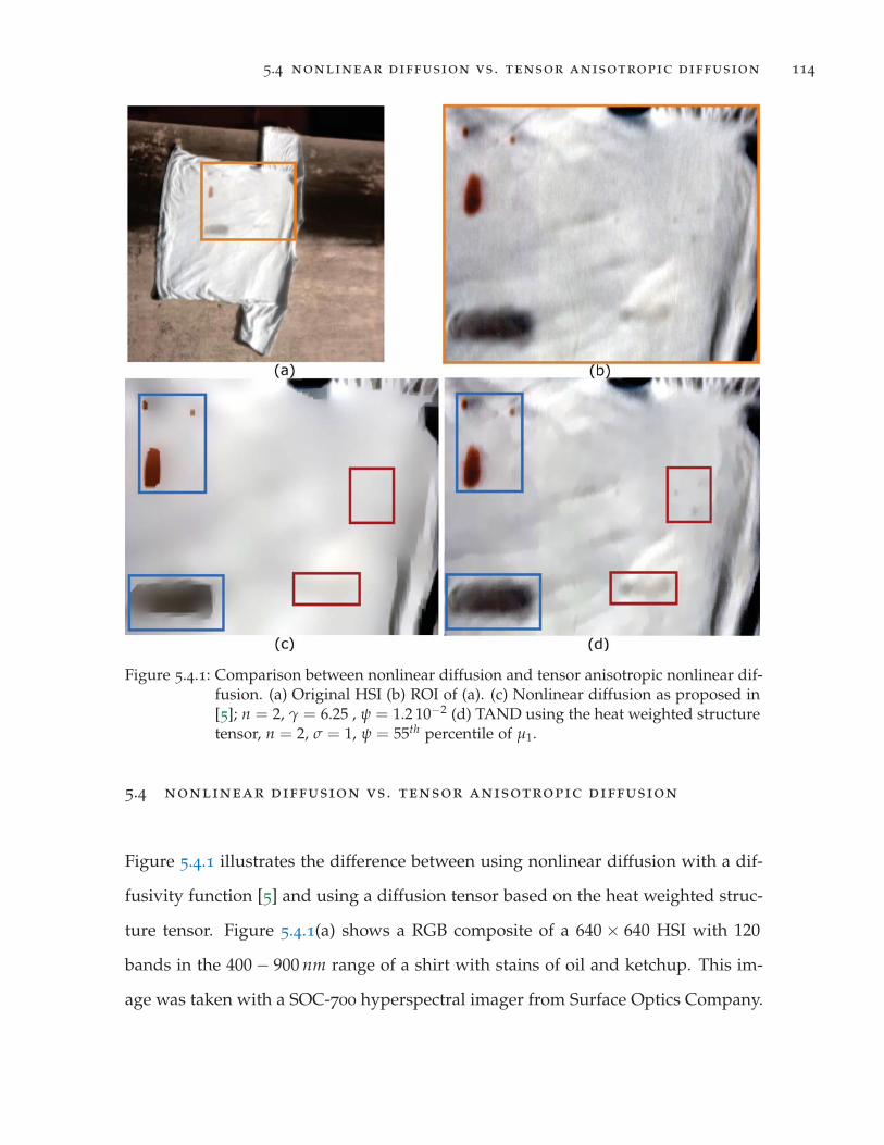
5.4 nonlinear diffusion vs . tensor anisotropic diffusion 114
Figure 5.4.1: Comparison between nonlinear diffusion and tensor anisotropic nonlinear dif-fusion. (a) Original HSI (b) ROI of (a). (c) Nonlinear diffusion as proposed in[5]; n = 2, γ = 6.25 , ψ = 1.2 10−2 (d) TAND using the heat weighted structuretensor, n = 2, σ = 1, ψ = 55th percentile of μ1.
5.4 nonlinear diffusion vs . tensor anisotropic diffusion
Figure 5.4.1 illustrates the difference between using nonlinear diffusion with a dif-
fusivity function [5] and using a diffusion tensor based on the heat weighted struc-
ture tensor. Figure 5.4.1(a) shows a RGB composite of a 640 × 640 HSI with 120
bands in the 400 − 900 nm range of a shirt with stains of oil and ketchup. This im-
age was taken with a SOC-700 hyperspectral imager from Surface Optics Company.

5.4 nonlinear diffusion vs . tensor anisotropic diffusion 115
Figure 5.4.1(b) shows the region of interest (ROI) inside of the orange square in
Figure 5.4.1(a) of size 184 × 225 where the stains are.
Figure 5.4.1(c) shows the ROI in Figure 5.4.1(b) after being denoised with the
PDE-based nonlinear diffusion proposed in [5]. This method uses the PDE in (2.4.1)
but instead of using a diffusion tensor D, it uses the diffusivity function in (4.2.1).
The PDE is discretized with a semi-implicit scheme that produces a five diagonal
linear system. This system is solved with a conjugate gradient method precondi-
tioned with incomplete Cholesky. The filtered image was produced with a Matlab
implementation provided by the authors of [5]. Figure 5.4.1(d) shows the denoised
image with TAND-EED using the heat weighted structure tensor. Figure 5.4.1(c)
used n = 2, γ = 6.25 , ψ = 1.2 × 10⁻² and Figure 5.4.1(d) used n = 2, σ = 1,
ψ = 55th percentile of μ1.
Usually PDE-based nonlinear diffusion is very good at preserving high contrast
edges as in the regions highlighted with blue squares in Figure 5.4.1(c). But low
contrast edges such as the ones highlighted in red are not preserved. Both kinds
of edges are preserved with the proposed TAND and in general there is a more
natural look to the image which preserves some wrinkles as well. Nonlinear diffu-
sion is the PDE-based diffusion algorithm of choice since it is computationally less
expensive than TAND, but the extra cost of TAND is justified by the quality of the
results.

5.5 comparison of the structure tensors using tand 116
5.5 comparison of the structure tensors using tand
5.5.1 TAND for Edge Enhancing Diffusion.
5.5.1.1 Experiments with A.P. Hill Image
Figure 5.5.1 shows the comparison of the structure tensors in TAND-EED using A.
P. Hill image with parametersσ = 1, τ = 5, ψ = μ′1s 45 percentile. The left col-
umn shows the results using the heat weighted ST and the right column using the
classical structure tensor. Figure 5.5.1(a) shows the λ−component of the diffusion
tensor for iteration n = 1, Figure 5.5.1 (b) shows the same component for iteration
n = 35, and Figure 5.5.1(c) shows the A. P. Hill image resulting after TAND-EED
with n = 35 iterations using the heat weighted structure tensor. Figure 5.5.1(d), (e),
and (f) show same images as in (a), (b), and (c) respectively but using the classical
structure tensor. From Figure 5.5.1(a) to (b) and Figure 5.5.1(d) to (e) it is clear that
the λ−component of the diffusion tensor have been smoothed with both structure
tensors and both preserve main features in the image. The blue squares in Figure
5.5.1(b) show features that the heat weighted structure tensor preserves while the
classical one does not. The results are very similar for both structure tensors in the
vegetation but the zoomed section of Figure 5.5.1(b) and (c) shows that the heat
weighted structure tensor preserves the features of the road for more iterations
while the classical structure tensor, shown in Figure 5.5.1(e) and (f), does not.
5.5.1.2 Experiments with Indian Pines image
Figure 5.5.2 shows the results of using TAND–EED with the classical structure ten-
sor (top row) and the heat weighted structure tensor (bottom row) for iteration
n = 1 (left column) and n = 4 (right column). With n = 4, TAND produces an
over-smoothed image that helps to visualize the time evolution of the diffusion

5.5 comparison of the structure tensors using tand 117
Figure 5.5.1: Comparison of the effect of the structure tensors in TAND-EED using A. P.Hill image. σ = 1, τ = 5, ψ = μ′
1s 45 percentile (a) λ−component of thediffusion tensor for iteration n = 1 using the heat weighted structure tensor.(b) λ−component of the diffusion tensor for iteration n = 35 using the heatweighted structure tensor. (c) A. P. Hill after TAND-EED n = 35. (d), (e), and(f) same as (a), (b), and (c) respectively but using the classical structure tensor.

5.5 comparison of the structure tensors using tand 118
Figure 5.5.2: False color of Indian Pines image after TAND-EED. σ = 0.8, ρ = 2, ψ =μ′
1s 55th percentile; (a) with the classical structure tensor, n = 1. (b) with theclassical structure tensor, n = 4. (c) with the heat weighted structure tensor,n = 1. (d) with the heat weighted structure tensor, n = 4.

5.5 comparison of the structure tensors using tand 119
Figure 5.5.3: Comparison of the effect of the structure tensor using the time evolution afteriterations n of the λ –entry of the diffusion tensor of TAND-EED applied toIndian Pines image. σ = 0.8, τ = 2, ψ = μ′
1s 55th percentile. (a) λ usingthe classical structure tensor, n = 1. (b) λ using the classical structure tensor,n = 4. (c) and (d) same as (a) and (b) using the heat weighted structure tensor.

5.5 comparison of the structure tensors using tand 120
Figure 5.5.4: Time evolution of the λ –entry of the diffusion tensor. σ = 0.8, τ = 2, ψ =μ′
1s 55th percentile, n = 3. (a) λ using the classical structure tensor; (b) λusing the heat weighted structure tensor; (c) original image with the mark upsections.
tensor. From Figure 5.5.2, it can be seen that both methods produce a smoothing
preserving the majority of the main edges. To better observe that the heat weighted
structure tensor produces better discrimination of structures that need to be persis-
tent through the iterations than the classical tensor, the λ−entry of the diffusion
tensor using both structure tensors will be shown and analyzed. Figure 5.5.3 shows
the evolution of the λ−entry of the diffusion tensor (see (4.1.2)) using the classical
and the proposed structure tensor. Both diffusion tensors use σ = 0.8, ρ = 2,
ψ = 55th percentile of μ1, and the eigenvalues defined in (4.2.1) and (4.2.2). Figure
5.5.3(a) and (b) show results using the classical structure tensor with n = 1 and
n = 4 respectively. Figure 5.5.3(c) and (d) show results using the heat weighted
structure tensor with n = 1 and n = 4 respectively.
It can be concluded that as a result of the nonlinear nature of TAND, the λ−entry
of the diffusion tensor has been smoothed: preserving the most important edges
and eliminating small variations in the homogeneous regions, as well as showing
the nonlinear nature of the structure tensor. Figure 5.5.4 shows a comparison be-
tween the λ−entry of the diffusion tensor after n = 3 iterations using the classical
and the proposed structure tensor. In both diffusion tensors, the same parameters

5.5 comparison of the structure tensors using tand 121
Figure 5.5.5: TAND–EED applied to FR1. σ = 0.5, τ = 1.2, ψ = μ′1s 50th percentile, n = 1
(a) original image; (b) using the classical structure tensor; (c) using the heatweighted structure tensor.
as in Figure 5.5.3 are used. Figure 5.5.4(a) shows λ using the classical structure
tensor. Figure 5.5.4(b) shows λ using the heat weighted structure tensor. Figure
5.5.4(c) shows the original image. The highlighted regions in the images corre-
spond in all three images. Highlighted regions in blue show that the diffusion ten-
sor using the heat weighted ST can preserve important structures longer, i.e., for
more iterations. Highlighted regions in green show several structures produced
by illumination changes preserved by λ using the classical structure tensor. Sev-
eral of those structures are still preserved in the next iteration; see Figure 5.5.3(b).
Highlighted regions in yellow show structures produced by illumination changes
preserved by λ using the heat weighted ST. Those pixels disappear in the next iter-
ation as can be seen in Figure 5.5.3(d). From Figure 5.5.4, it can be concluded that
the heat weighted structure tensor enhances the capabilities of the diffusion tensor
to discriminate which edges are more important to keep.
5.5.1.3 Experiments with Forest Radiance 1 Image
To process FR1, it is necessary to smooth the image, since there are vertical textures
from the grass. But the smoothing cannot be too strong or it will erase the sub-
pixel targets. Figure 5.5.5 shows false color images resulting from TAND for EED
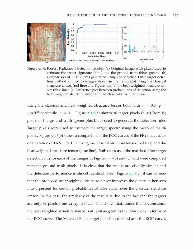
5.5 comparison of the structure tensors using tand 122
Figure 5.5.6: Forrest Radiance 1 detection results. (a) Original Image with pixels used toestimate the target signature (blue) and the ground truth (blue+green). (b)Comparison of ROC curves generated using the Matched Filter target detec-tion method applied to images shown in Figure 5.5.5(b) using the classicalstructure tensor, (red line) and Figure 5.5.5(c) the heat weighted structure ten-sor, (blue line). (c) Difference plot between probabilities of detection using theheat weighted structure tensor and the classical structure tensor.
using the classical and heat weighted structure tensor both with σ = 0.5, ψ =
μ′1s 50th percentile, n = 1 . Figure 5.5.6(a) shows 26 target pixels (blue) from 84
pixels of the ground truth (green plus blue) used to generate the detection rules.
Target pixels were used to estimate the target spectra using the mean of the 26
pixels. Figure 5.5.6(b) shows a comparison of the ROC curves of the FR1 image after
one iteration of TAND for EED using the classical structure tensor (red line) and the
heat weighted structure tensor (blue line). Both cases used the matched filter target
detection rule for each of the images in Figure 5.5.5(b) and (c), and were compared
with the ground truth pixels. It is clear that the results are visually similar and
the detection performance is almost identical. From Figure 5.5.6(c), it can be seen
that the proposed heat weighted structure tensor improves the detection between
1 to 7 percent for certain probabilities of false alarm over the classical structure
tensor. In this case, the similarity of the results is due to the fact that the targets
are only 84 pixels from 21025 in total. This shows that, under this circumstance,
the heat weighted structure tensor is at least as good as the classic one in terms of
the ROC curve. The Matched Filter target detection method and the ROC curves
5.5 comparison of the structure tensors using tand 123
values were generated using the ENVI software. The next section will show that
for a more challenging problem, the heat weighted structure tensor produces better
results than the classic structure tensor.
5.5.1.4 Experiment with Cuprite Image
Figure 5.5.7 shows the λ−component of the diffusion tensor for the Cuprite image.
Left column shows results of the proposed TAND-EED using the heat operator ST
and the right column shows results of the proposed TAND-EED using the classical
ST. Comparing for n = 1 in Figure 5.5.7 (a) and (d) the heat weighted structure
tensor helps the diffusion tensor to preserve the roads and other important features
while the classical ST does not. When the proposed TAND-EED using the heat
weighted ST iterates, as shown in Figure 5.5.7(b) for n = 5 and (d) for n = 15,
preserves the roads and the different materials smoothing its homogeneous regions
and not its edges. On the other hand, the proposed TAND-EED using the classical
structure tensor, shown in Figure 5.5.7(e) for n = 5 and (f) for n = 15 does not. This
fact is more notorious in the time evolution shown in Figure 5.5.8 where the results
of the proposed TAND-EED are shown for the same images as in Figure 5.5.7
5.5.2 TAND for Coherence Enhancing Diffusion.
5.5.2.1 Thyroid Cells Image.
To show the performance of CED with the heat weighted structure tensor for an
image with complex small structures, the thyroid tissue image is used. It is difficult
to evaluate this image by inspecting the diffusion entries of the diffusion tensor so
the evaluation will be done by studying its evolution through the iterations. Figure
5.5.9 shows the thyroid tissue image processed using the classical structure tensor
in the left column and the heat weighted structure tensor in the right column. The

5.5 comparison of the structure tensors using tand 124
Figure 5.5.7: Comparison of the effect of the structure tensor using the time evolution ofthe λ−entry of the diffusion tensor of TAND-EED applied to Cuprite image.σ = 1, τ = 5, ψ = μ′
1s 45 percentile (a) n = 1 using the heat weightedstructure tensor. (b) n = 5 using the heat weighted structure tensor. (c) n = 15using the heat weighted structure tensor. (d), (e), and (f), are the same as (a),(b), and (c) respectively but using the classical structure tensor.

5.5 comparison of the structure tensors using tand 125
Figure 5.5.8: Comparison of the effect of the structure tensor using the time evolution ofthe resulting images of TAND-EED applied to Cuprite image. (a) n = 1 usingthe heat weighted ST; (b) n = 5 using the heat weighted ST; (c) n = 10 usingthe heat weighted ST; (d) n = 15 using the heat weighted ST; (e), (f), (g), and(h) same as (a), (b), (c), and (d) respectively but using the classical ST.
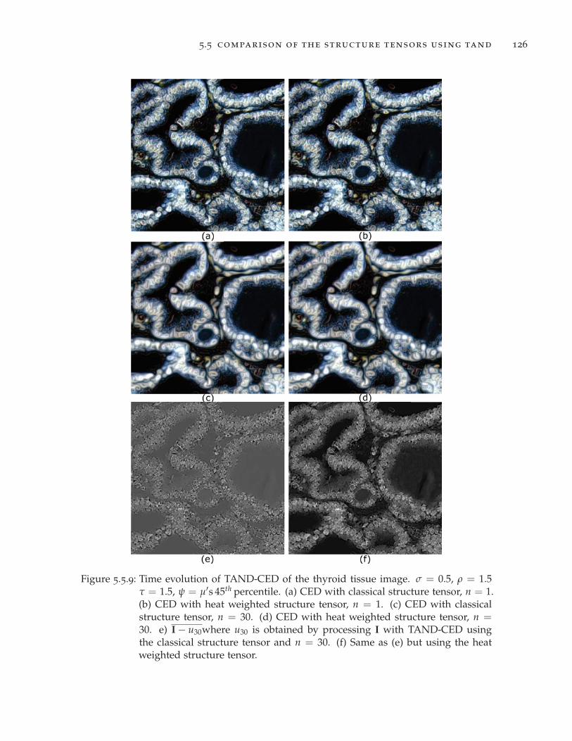
5.5 comparison of the structure tensors using tand 126
Figure 5.5.9: Time evolution of TAND-CED of the thyroid tissue image. σ = 0.5, ρ = 1.5τ = 1.5, ψ = μ′s 45th percentile. (a) CED with classical structure tensor, n = 1.(b) CED with heat weighted structure tensor, n = 1. (c) CED with classicalstructure tensor, n = 30. (d) CED with heat weighted structure tensor, n =30. e) I − u30where u30 is obtained by processing I with TAND-CED usingthe classical structure tensor and n = 30. (f) Same as (e) but using the heatweighted structure tensor.

5.5 comparison of the structure tensors using tand 127
first row shows results for iteration n = 1. The middle row shows results for n = 30.
Notice that, from n = 1 to n = 30, the edges of the cells have been thickened and
the homogeneous regions show a light smoothing. Subtracting the image resulting
from CED after n = 30 iterations, u30, from the original image I, produces an
image with 224 bands. This image is averaged over all bands, i.e., I − u30. Figure
5.5.9(e) shows it using the classical structure tensor and Figure 5.5.9(f) using the
heat weighted structure tensor. These images are displayed with the intensity range
set to [min I − u30, maxI − u30]. Figure 5.5.9(f) has higher contrast between cell
edges and dark regions. The next step is to use a threshold, φ, equal to a user
defined percentile of the intensity values of I − u30, i.e. for n = 30,
In,φ = I − un|φ . (5.5.1)
The results, using φ = 75th percentile, are the binary images shown in Figure
5.5.10. Figure 5.5.10(a) shows I30,75 using the classical structure tensor while Fig-
ure 14(c) shows it using the heat weighted structure tensor. Figure (5.5.10)(b) and
(d) show I30,75 after eliminating all the connected components with area less than
or equal to 15 pixels (called granules) using the morphological operator open in
the Matlab function bwareaopen. Figure 5.5.10(b) uses the classical structure tensor
and Figure 5.5.10(d) uses the heat weighted structure tensor. The images in Fig-
ure 5.5.10(b) and (d) show a better definition of the individual cells. Comparing
the values of I30,75 in Figure 5.5.10(a) and (c), it can be seen that I30,75 using the
heat weighted structure tensor (bottom row) has fewer granules, and the cells look
more complete. To quantify these observations, a test was designed in which I30,φ
is calculated with values of φ taken every second percentile from the 30th to the
98th percentile. Values of φ less than the 30th percentile show too much detail to ef-
fectively count the cells. For each value of φ, the number of connected components

5.5 comparison of the structure tensors using tand 128
Figure 5.5.10: Edges enhanced by TAND–CED. (a) using the classical structure tensor, I30,75as defined in (5.5.1). (b) Same as (a) after eliminating all granules of area 15pixels. (c) Same as (a), but using the heat weighted structure tensor. (d) Sameas (b), but using the heat weighted structure tensor.

5.5 comparison of the structure tensors using tand 129
Figure 5.5.11: Comparison of number of granules of I30,φ with area less than equal to 15 pix-els found using the classical structure tensor vs. the heat weighted structuretensor.
with an area of 15 pixels or less is counted. Then a ratio, r between the number
of granules found in I30,φ for the classical structure tensor, GC, and the number of
granules in I30,φ for the heat weighted structure tensor, GH, is calculated, i.e.,
r = GC/GH.
If GC = GH then r = 1; if GC > GH then r > 1, and if GC < GH then 0 < r < 1. The
results are shown in Figure 5.5.11.
After the 36th percentile, the number of granules for the classical structure tensor
is higher than the number of granules for the heat weighted structure tensor. At the
42nd percentile, the one based in the classical structure tensor has almost 2.5 times
the number of granules than the proposed method. This decreases to 1.4 times as
many at the 60th percentile before growing to almost 1.9 at the 86th percentile. Cell
counting is an important application for these images. To that end, φ in [70th, 85th]
percentile is one of the most critical intervals since In,φ will begin to show the cells
separating from each other. As the value of φ gets higher, many cells will look
incomplete and the resulting images are less critical.

5.6 comparison between the spectrally adapted and weickert’s spatial tand. 130
From Figure 5.5.11, it can be seen that between the 70th and 85th percentile, I30,φ
for the classical structure tensor has between 1.6 to 1.9 times the number of gran-
ules of the proposed method. Therefore, weighting the structure tensor using the
weights based on the heat operator helps TAND to make a better distinction be-
tween the cells edges and their surrounding features.
5.6 comparison between the spectrally adapted and weickert’s spa-
tial tand.
In the previous section, comparisons were done preserving the proposed TAND
and only changing the structure tensor. The idea was to study the performance
of the proposed structure tensor compared with the classical one. In this section,
TAND with the spectrally adapted structure tensor and the proposed diffusion
tensors will be compared to the state of the art TAND proposed by Weickert [2].
5.6.1 TAND for Edge Enhancing Diffusion
A time step τ = 5 and number of iteration, n = 4 will be used for EED. That is
equivalent to 80 iterations of the explicit scheme which is empirically stable for
time step size of at most τ = 0.25 [46]. Figure 5.6.1 shows the results of this
comparison. Figure 5.6.1(b), (d), (e) and (f) show results from Weickert’s TAND
and Figure 5.6.1(c), (g), (h) and (i) show the proposed TAND. Weickert’s TAND
shows a strong smoothing in the whole image preserving only the strongest edges.
The edges look blurry and the small features are hardly visible. In contrast, the
proposed TAND the edges are not blurred and the smoothing in the inside regions
is visually comparable to Weickert’s. The small features are still visible and remind
with the same color composition than in the original image. A shock filter to

5.6 comparison between the spectrally adapted and weickert’s spatial tand. 131
Figure 5.6.1: Comparison of the regularization from proposed TAND and Weickert’s TAND.σ = 0.8, τ = 5, ψ = μ′
1s 55th percentile, n = 4. (a) RGB Indian Pines image (b)after Weickert’s TAND (c) after proposed TAND; (d), (e) and (f) are λ, β, and νcomponents of Weickert diffusion tensor. (g), (h) and (i) are the correspondingcomponents of the proposed diffusion tensor.

5.6 comparison between the spectrally adapted and weickert’s spatial tand. 132
unsharp the edges is usually used after diffusion . For the case of the proposed
TAND, this is not need it. This difference is explained with the components of
their respective diffusion tensors. Figure 5.6.1(e) and (h) shows the β− component
of both methods. It is clear that, for Weickert, this component plays an important
role. While in the case of the proposed TAND does not. According to the analysis
of the divergence-based PDE diffusion carry out by [3] β produce an inter channel
coupling which is reduced in the proposed TAND. λ and ν− components of the
proposed TAND looks very similar but their values for the horizontal and vertical
edges are different. So depending in the application, preserving the edges can
help to obtain better results for the next processing in the image. Comparison with
Figure 5.6.2 and Figure 5.6.3 show similar conclusions than the ones with Figure
5.6.1.
5.6.2 TAND for Coherence Enhancing Diffusion
The thyroid cell tissue will be used for the comparisons for CED. The parameters
used are: time step size τ = 5, σ = 0.5, ρ = 2.5 and n = 30. Figure 5.6.4 shows the
thyroid tissue being processed with Weickert’s TAND and the proposed TAND. It
is clear the the proposed TAND produce less enhancement of the area around the
cell chain and produce less granules as shown in Figure 5.6.5.

5.6 comparison between the spectrally adapted and weickert’s spatial tand. 133
Figure 5.6.2: Comparison of the proposed TAND-EED with Weickert’s TAND-EED appliedto Cuprite image. (a) n = 1 using the proposed TAND; (b) n = 5 using the theproposed TAND-EED; (c) n = 15 using the proposed TAND; (d), (e), and (f)are the same as (a), (b), and (c) respectively but using the Weickert’s TAND.

5.6 comparison between the spectrally adapted and weickert’s spatial tand. 134
Figure 5.6.3: Comparison of the proposed TAND-EED with Weickert’s TAND-EED appliedto A. P. Hill image. Both methods uses σ = 1.5, τ = 5, ψ = μ′
1s 45 percentile.(a) n = 1 using the proposed TAND; (b) n = 15 using the the proposed TAND-EED; (c), and (d) same as (a) and (b) respectively but using the Weickert’sTAND.

5.6 comparison between the spectrally adapted and weickert’s spatial tand. 135
Figure 5.6.4: Comparison of cell chains obtained with the spectrally adapted TAND andWeickert’s TAND. τ = 5, σ = 0.5, ρ = 2.5 and n = 30. (a) I30,75 using theclassical structure tensor, as defined in (5.5.1). (b) Same as (a), after eliminat-ing all granules of area 15 pixels. (c) I − u30 with Weickert’s TAND-CED (d)I30,75 using the heat weighted structure tensor. (e) Same as (d) after eliminat-ing all granules of area 15 pixels. (f) I − u30 with proposed TAND-CED, (g)Weickert’s TAND-CED (h) Proposed TAND-CED (i) Original Image

5.7 concluding remarks 136
Figure 5.6.5: Comparison of number of granules of I30,φ with area less than equal to 15 pix-els found using the classical structure tensor vs. the heat weighted structuretensor.
5.7 concluding remarks
The experiments in this chapter show that defining the weights with s = 1 pro-
duces more stable results for CED than variying s with the number iterations, n, of
TAND. They also show that using an anisotropic diffusion based on a tensor helps
the diffusion process to discriminate and ultimately preserve low contrast edges.
Comparing the ST using TAND show that the heat weighted structure tensor helps
the diffusion tensor TAND-EED to better discriminate which edges to keep longer
as TAND-EED iterate. This result was achieved by comparing the components of
the diffusion tensor of TAND-EED produced using the proposed heat weighted
and the classical structure tensor. The proposed ST also helps TAND-CED to pro-
duce less broken edges and to obtain a better structure enhancement than using
the classical structure tensor. From the comparison between the proposed TAND
with Weickert’s TAND, it can be concluded that the proposed ST produce better
regularization results since the edges are not blurred while the inner regions are
strongly smoothed but preserving the small features in the images. Comparing

5.7 concluding remarks 137
both TAND-CED can be concluded that using the heat weighted ST applied to the
thyroid cell image produces less broken edges and the chain of cells can be better
discriminated than using Weickert’s TAND-CED.

6O N P U B L I C LY AVA I L A B L E R E M O T E S E N S I N G I M A G E RY
The work presented in this thesis belongs to the Hyperspectral Remote Sensing
field. The discussion in this chapter will be expanded to include aerial photography
and satellite imaging in general. This chapter will reflect on and present issues
about the impact of publicly available remotely sensed imagery.
A brief overview of the advances in technology and some events that helped
reach the availability of remotely sensed data to the public will be presented. It is
not by any means complete. It is done with the aim of placing ideas in perspec-
tive. The first launch of a non-weather satellite for civilian use occurred in 1972
when NASA put Landsat into orbit to monitor the planet’s land masses, tracking
everything from desertification to changes in agriculture. During the 1980s, hyper-
spectral remote sensors were developed. Satellites with the capability of acquiring
HSIs were launched in the subsequent decades, bringing more analytic capabilities
to the data collected. At the same time geospatial data began to be developed but
it was not until the mid-2000s that this technology began have its greatest impact
on our society. Geospatial data is the combination of several technologies such as
remote sensed data, GIS and global positioning systems (GPS). Geospatial data add
high positional accuracy capabilities to the remotely sensed data, in that way inte-
grating separate or loosely related technologies producing a powerful system [110].
Another factor was the the creation of the global information infrastructure, i.e.,
the development and public access to the Internet for the majority of people on the
planet. The internet allows access to information in nearly real time. With the de-
138

on publicly available remote sensing imagery 139
velopment of computer hardware, cheap computer memories and wide broadband
internet access, now it is possible to download a high volume of data in several
minutes.
Fourteen years ago, in 1998, several ethical issues were raised by [111] related
to the advances in (i) information management, data control of remotely sensed
imagery, and (ii) the development of a digital, global information infrastructure,
such as the Internet. There were concerns about the usage of remotely sensed data
given the general evolution of the remote sensing infrastructure from government
to commerce and from domestic to international. This paper also warned about the
lack of comprehensive policy development with respect to high-resolution remote
sensing technology. The relaxed policies about remotely sensed data paved the way
for Google Earth that was launched in 2005.
This brought about the change from centralized government owned remotely
sensed data to freely acquired aerial imagery using Google Earth and from data
produced by trained experts and then processed to be used for another set of
trained experts to data openly available to anybody who knows how to use the
internet. Google Earth uses high spatial resolution data provided by commercial
satellite image providers like DigitalGlobe and GeoEye as well as data provided
by local municipalities and governmental agencies [112]. Not only Google can
acquire remotely sensed imagery, nowdays it is possible to market, sell and buy
high spatial and spectral resolution global imagery. The USA, Russian, French,
Japanese, Indian, Chinise-Brazilian, Israel and Canadian governments, and even
non-goverment parties sell this kind of imagery acquired by their orbiting imaging
system over the Internet [110, 113]. According to a United Nation resolution for re-
motely sensed data [114], data rights, pricing, and distribution policies reside with
the governments owning the spacecraft.

on publicly available remote sensing imagery 140
All that gives rise to issues about privacy. Those images are acquired without tak-
ing into account the owner of the land being sensed or any wishes for privacy that a
person or institution might have. Of course, if it were necessary to have the written
permission of every owner of a piece of land in the Earth, Remote Sensing would
not exist. Despite the fact that global remote sensing requires some form of global
rules, the addition of profitable businesses ruled by market variables and civilian
and military interests make it very difficult to have meaningful rules governing it
[113]. So, now it is possible to have access to high spatial resolution photographs of
military installations (national or foreign) and study its development through the
years [115]. It is also possible to acquire high spatial and spectral HSI images de-
tecting hidden precious metal deposits and to then sell them to the highest bidder
without the owner of the land even knowing it. This is somewhat extreme as you
normally need some idea of where to look but it is possible. Definitely it is possible
to open Google Earth in any random place in the US click Street View and maybe
within five minutes or so you can see the state of the neighborhood and then send
advertisements of your products. It is also possible to find a picture of a car clearly
showing its license plate in the driveway of a random house. All the before men-
tioned factors have contributed to us living in a surveillance society. For example
questions, such as: Can the IRS use those images to look for unreported property
renovation or extension? Can the law enforcement and environmental agencies use
these publicly available images to do surveillance without a warrant? The answer
is yes at least in the US [111, 113] and Canada [116].
Another interesting issue raised by [115] related to Google Earth and to some
extend to all remotely sensed imagery is the idea of a ‘global panopticon’ in which
the viewer of data sees all, but those who are viewed see nothing and, importantly,
do not know if and when they are being watched. Furthermore, the majority of
those being viewed are not even aware of the mechanism that might be watching

6.1 concluding remarks 141
them and correspondingly do not act as if they are being watched. So there are two
faces of the coin, the liberating and revelatory aspects of this technology unveiling
governments and military to all and in contrast the possibly repressive aspects of a
panoptic technology of surveillance.
On a brighter side, public access to remote sensing imagery has allowed some
non-environmentally or non-military related projects that are looking for the greater
good for humanity. The use of remotely sensed images as evidence of human rights
violations, such as the ones in Darfur and Zimbabwe [117]. They have also been
used to investigate accusations of human rights violations, such as government
sponsored forced relocation, location of massive graves, and to document the ex-
tent of conflicts in many parts of the world [118, 119]. HSIs have been used in
environmental applications since its development. But now not only satellite im-
agery is used but high resolution spacial aerial images found freely in Google Earth
have also been used to make virtual discoveries. Hundreds of new species in dense
and difficult to access forests in different parts of the world have been found us-
ing the available imagery, which then led to an in-site discovery. The internet and
remotely sensed imagery is also used to create awareness to all that are willing to
read about the speed of deforestation on some other part of the planet [120].
6.1 concluding remarks
In conclusion, publicly available remote sensing imagery has issues related to pri-
vacy, data management and control of who owns the information. The reality of
being sensed from so many feet over our heads and not knowing it produces the
idea of a panoptic society in which even the governments cannot hide its secrets
places. On the other hand, the fact that everybody who owns a computer and uses
internet can have access to it also gives some liberating sense. In general, it is diffi-

6.1 concluding remarks 142
cult to control the flow of remotely sensed information since many parties produce
it and distribute it. On the other hand, it has been shown that there is more avail-
ability of data for the experts and for people who just like to be informed. It is also
expected advances in the creation of sensors with more capabilities, now that there
is a wider use of remotely sensed technology.

7C O N C L U S I O N S A N D F U T U R E W O R K
7.1 conclusions
The structure tensor is the backbone in many algorithms used in computer vision
to find the spatial local structure in color and gray value images. Its extension to
vector valued images with more than 3 bands has been done without taking into
account the spectral characteristics of the data. The structure tensor is a useful
tool that arises in many frameworks such as statistics, differential geometry, and
optimization. This work showed that including the spectral information in the
structure tensor makes a difference and it can improve significantly image enhance
methods such as TAND.
A spectrally weighted structure tensor framework has been presented. Also, a
spectrally weighted structure tensor for the case of vector-value images that locally
are highly correlated in the spectral dimension has been proposed. The weights
are based on the heat operator acting on each pixel of the gradient. This structure
tensor is data-based and it does not introduce new parameters to the model.
Diffusion tensors were proposed and it was shown that they take full advantage
of the edge information produced by the spectrally weighted structure tensor. The
proposed diffusion tensors were used to design a Tensor Anisotropic Nonlinear Dif-
fusion (TAND) for Edge Enhancing Diffusion (EED) and for Coherence Enhancing
Diffusion (CED). TAND-EED was used to regularize HSIs, while TAND-CED was
used to do structure enhancement. Experiments with HSI of different spatial and
143

7.1 conclusions 144
spectral resolutions were used. The images were taken using sensors in airborne,
microscope, and in-situ hyperspectral camera. The experiments compare the pro-
posed TAND using the heat weighted structure tensor with the proposed TAND
using the classical structure tensor.
The experiments performed in this work showed that the proposed weighted
structure tensor enhanced the ability of the diffusion tensor of TAND–EED to dis-
criminate edges that must persist longer through the iterations while discarding
edges that are less important. To the best to my knowledge, TAND–CED has not
been used before to do structure enhancement of HSIs. Neither is used to do
structure enhancement of HSI as treated in this work. TAND–CED using the heat
weighted structure tensor produced less broken edges than the one using the classi-
cal structure tensor. In this case, two different problems from different fields were
treated. One was extracting the chain of cells in a thyroid tissue image and the
other was finding the wakes of a boat in an open ocean image. This was achieved
by averaging along the spectral direction the image of the difference between the
original image and the TAND-CED processed image at some iteration n. Counting
the number of connected components of small area of the resulting image was used
as a measure of how broken the edges were. Then the ratio, r, between the numbers
of granules found using the classical ST over the number of granules found using
the heat weighted one was used to assess performance. The graph of r vs. φ (the
threshold for the intensity values of the averaged image) in both problems showed
that TAND-CED using the heat weighted ST produces less broken edges.
About the convergence of the nine diagonal linear system it was found that
ILU(0) was enough to accelerate the convergence of the solution.

7.2 future work 145
7.2 future work
The spectrally adapted structure tensor presented in Chapter 3 is designed for
vector-valued images that are locally highly correlated, such as HSI. Finding a way
to spectrally adapt other kind of vector-valued images, such as MSI, that do not
fully or partially fulfill this condition is important, so TAND can be adapted to
them. The spectrally adapted structure tensor can be studied also for 3D images,
i.e., volumetric images, such as MRI medical images.
Finding a tensor for TAND that produce less or none rounding effect in the
corners is another topic to study. This effect is due to the fact that the structure
tensor for EED does not distinguish between right and left directions. This is a
known problem, it have been studied by Steidl and Teuber for gray value images
of shear and rotated rectangles [121]. In this case, they modify the eigenvectors of
the structure tensor to make them sensible to directions, and not only orientations.
A diffusion tensor that mitigates this problem for images with shear and rotated
rectangles is also proposed. So, an study of an spectrally adapted structure tensor
that it is sensible to directions to try the correct the rounding of the corners can also
be done. Another direction of study is the usage of structure tensor-based corners
detection methods and used it to correct the lack of detection of the corners by the
structure tensor itself.
From the implementation of the structure tensor, it is clear that all the operations
are done pixel-wise. To calculate the structure tensor per pixel, it is only necessary
the pixel and its 3 × 3 neighborhood around itself. This produces an embarrassing
parallel scenario. So a parallel implementation can be done. TAND on the other
hand has the same characteristics until the step in which the linear system need to
be solved. There are parallel implementations of BiCGStab for distributed memory
architectures. In [122], a parallel implementation using Compute Unified Device
7.2 future work 146
Architecture (CUDA) in Graphics Processing Unit (GPU) have been proposed for
solving finite difference linear systems with explicit preconditioned Biconjugate
Conjugate Gradient type methods . So a parallel implementation of the structure
tensor and TAND can be achieved.
Studying the effect of the disturbance term presented in Section 4.5 thru the
iterations and its real impact in the divergence-based diffusion can be another study
direction. A study of advantage and disadvantage of using TAND-EED versus
using the regularization obtained using the trace-base diffusion operator presented
by [123, 3] for HSI can be useful to study in which situation is better to use either
method.

A P P E N D I X
147

AS E L E C T E D T O P I C S
a.1 some definitions from linear algebra and numerical analysis
The definitions in this section are based on the ones appearing in [102].
a.1.1 Rank of a Matrix
The rank of a matrix A is defined as the dimension of the subspace for which
Tv �= 0 and denoted by rank. The space for which Tv = 0 is known as the null space.
The dimension of the null space is known as nullity, denoted by null. One of the
most important theorems in linear algebra, known as dimension theorem establish
that:
rank(A) + null(A) = d
where d is the number of columns of A, which in the case of symmetric matrices is
the same as its number of rows.
a.1.2 Sparse and dense Matrices
A sparse matrix is a matrix in which the majority of entries are zero. In contrast, a
dense matrix is one in which the majority of the entrances are non-zero. A structured
sparse matrix is one whose nonzero entries form a regular pattern, often along a
148

A.1 some definitions from linear algebra and numerical analysis 149
small number of diagonals. A matrix with irregularly located entries is said to be
irregularly structured. One way to produce sparse matrices is from the discretization
of a PDE or an Ordinary differential equation (ODE) to fit the continuous theory
into the discrete data.
a.1.3 Projection Methods to solve large linear systems
Given a linear system
Ax = b (A.1.1)
where A is a k × k real matrix. A can also denote the linear mapping in Rk that it
represents. b is a vector with the same number of rows as A, and x is the solution
vector to be found when solving the linear system (A.1.1) . The idea of projection
methods is to extract an approximate solution to the above problem from a subspace
K of Rk.
The Petrov-Galerkin conditions are m (independent) orthogonality conditions im-
posed over the the search subspace K of dimension m so an approximate solution
of (A.1.1) can be found in K. Specifically, the residual vector b − Ax is constrained
to be orthogonal to m linearly independent vectors. This defines another subspace
L of dimension m which will be called the subspace of constraints . This is,
Find x ∈ K, such that b − Ax ⊥ L
when an initial guess x0 to the solution exists then the approximation must sought
in the affine space x0 + K instead of the homogeneous vector space K. Then the
problem becomes
Find x ∈ x0 +K, such that b − Ax ⊥ L.

A.1 some definitions from linear algebra and numerical analysis 150
Figure A.1.1: Interpretation of the orthogonality condition. Taken from [102]
x ∈ x0 + K means that x can be written as x = x0 + δ, for some δ ∈ K. Let the
residual vector r0 be defined as :
r0 = b − Ax0, (A.1.2)
then
b − A (x0 + δ) ⊥ L or r0 − Aδ ⊥ L
then by definition of orthogonality the approximate solution can be defined as:
x = x0 + δ, for δ ∈ K, such that 〈r0 − Aδ, w〉 = 0, ∀w ∈ L
where 〈·, ·〉 is the inner product defined in Rm.
Many of the standard techniques use a succession of these projections. Typically,
a new projection step uses a new pair of subspaces K and L and an initial guess x0
equal to the most recent approximation obtained from the previous projection step
[102]. When K = L then the projection method is known as orthogonal, otherwise
oblique. This distinction is rather important and gives rise to different types of
algorithms.

A.1 some definitions from linear algebra and numerical analysis 151
A set of methods known as Krylov subspace methods defines the search subspace
K of dimension m as
Km (A, r0) = span{
r0, Ar0, A2r0, ..., Am−1r0
}
where r0 is defined as in (A.1.2). The different Krylov methods distinguish one
from another by the definition of Lm and the use of preconditioners.
For completeness in the presentation the three most used Krylov methods used
for non-symmetric linear systems will be presented in the next subsections all the
algorithms are taken from [102].
a.1.3.1 BiCG
Bi-conjugated gradient, BiCG, is a Krylov method that solves non-symmetric linear
systems by defining a projection process onto
Km = span{
v1, Av1, A2v1, ..., Am−1v1
}
orthogonal to
Lm = span{
w1, ATw1,(
AT)2
w1, ...,(
AT)m−1
vw
}
with v1 = r0/ ‖r0‖2 and w1 an arbitrary vector that fulfills 〈v1, w1〉 �= 0. w1 = v1
is often chosen. If there is a dual system ATx∗ = b∗ to be solved with AT then
v1 = r∗0/ ‖r∗0‖2 where r∗0 = b∗ − ATx∗0. The algorithms is presented in Algorithm
A.1 [102]. If a dual system with AT is being solved then r∗0 = b∗ − ATx∗0 and the
update x∗j+1 := x∗j + αj p∗j to the dual approximate solution must be added after
line 5 in Algorithm A.1. There is a variant of this algorithm that avoid the products
with the transpose matrix which is a more efficient computationally.

A.1 some definitions from linear algebra and numerical analysis 152
Algorithm A.1 Bi-Conjugate Gradient (BiCG)
1. Compute r0 = b − Ax0. Choose r∗0 such that 〈r0, r∗0〉 �= 0.
2. Set, p0 = r0, p∗0 = r∗0
3. For j = 0, 1, ..., until convergence do
4. αj :=
⟨rj,r∗j
⟩⟨
Apj,p∗j⟩
5. xj+1 := xj + αj pj
6. rj+1 := rj − αj Apj
7. r∗j+1 := r∗j − αj Ap∗j
8. β j :=
⟨rj+1,r∗j+1
⟩⟨
rj,r∗j⟩
9. pj+1 := rj+1 + β j pj
10. p∗j+1 := r∗j+1 + β j p∗j
11. EndDo

A.1 some definitions from linear algebra and numerical analysis 153
Algorithm A.2 BiCGStab
1. Compute r0 = b − Ax0. Choose r∗0 arbitrarily
2. Set, p0 = r0
3. For j = 0, 1, ..., until convergence do
4. αj :=
⟨rj,r∗j
⟩〈Apj,r∗0〉
5. sj := rj − αj Apj
6. ωj := 〈Asj,sj〉〈Asj,Asj〉
7. xj+1 := xj + αj pj + ωjsj
8. rj+1 := sj − ωj Asj
9. β j := 〈rj+1,r∗0〉〈rj,r∗0〉 × αj
ωj
10. pj+1 := rj+1 + β j(
pj − ωj Apj)
11. EndDo
a.1.3.2 BiCGStab
Bi-Conjugate gradient method was developed to avoid the usage of the transpose
of A in BiCG and to gain faster convergence. This method check for convergence
twice in one iteration, so the method can converge in the middle of an iteration.
The algorithm is presented in Algorithm (A.2)
a.1.3.3 GMRES
The Generalized Minimum Residual Method (GMRES) is a projection method based
on taking K = Km and L = AKm in which Km is the m − th Krylov subspace with

A.1 some definitions from linear algebra and numerical analysis 154
Algorithm A.3 GMRES
1. Compute r0 = b − Ax0. β := ‖r0‖2, and v1 = r0/β
2. For j = 0, 1, ..., m Do:
3. Compute wj := Avj
4. For i = 0, 1, ..., j Do:
5. hij :=⟨wj, vi
⟩6. wj := wj − hijvi
7. EndDo
8. hj+1 :=∥∥wj∥∥
2. If hj+1,j = 0 set m := j and go to 11
9. vj+1 = wj/hj+1, j
10. EndDo
11. Define the (m + 1)× m Hessenberg matrix Hm ={
hij}
1≤i≤m+1,1≤j≤m.
12. Compute ym the minimizer of ‖βe1 − Hmy‖2 and xm = x0 + Vmym.
v1 = r0/ ‖r0‖2. This technique minimizes the residual norm over all vectors in
x0 +Km. Any vector in x0 +Km can be written as
x = x0 + Vmy,
where y is an m−vector.The simplest version of this algorithm is presented in Table
(A.3) [102].
BA P R E C O N D I T I O N E R F O R S O LV I N G T H E F I N I T E
D I F F E R E N C E D I S C R E T I Z AT I O N O F P D E S A P P L I E D T O
I M A G E S
b.1 linear systems and preconditioners used to solve them
Semi-implicit schemes are the most common methods used in PDE-based image
processing [2, 5, 4]. These schemes produce a linear system that need to be solved
in each iteration. Depending on the discretization those system can suffer from
slow convergence. The mathematical guarantees are, at best, that the solution can
be found in linear time that depend on the number of entries in the image. For
high dimensional data such as HSI, this can be really slow. Therefore the most
common practice to accelerate convergence is preconditioning the coefficient ma-
trix. Preconditioning are a set of methods that find equivalent linear systems with
the same solution that the original linear system. This is done by transforming
the original linear system into one that has the same solution, but it is likely to be
easier to solve with an iterative solver [102].
For example, the system Ax = b can be transformed by :
M−1Ax = M−1b (B.1.1)
or
AM−1u = bM−1 (B.1.2)
155

B.1 linear systems and preconditioners used to solve them 156
where M−1 can be obtained using some analytical method or the solution of a sub-
sidiary linear system u = Mx. (B.1.1) is known as left-preconditioner and (B.1.2) as
right-preconditioner. Usually explicit computation of M and M−1A will be avoided.
Instead the iterative processes operate with A and M−1 whenever it is necessary.
The most simple explicit preconditioner technique is given by the Jacobi or diag-
onal preconditioner. This preconditioner consist in setting the preconditioner M =
diag(A), assuming that Aii �= 0 for all i. The system is solved by a Krylov method.
The standard preconditioner is the one obtained by the incomplete factorization of
the original matrix A. The coefficient matrix A is factored into the product of the
lower triangular and upper triangular parts of A denoted respectively as L and U,
and the residual or error of the factorization R is subtracted, that is:
A = LU − R
this factorization is known as ILU(0). It is rather popular since it is easy and inex-
pensive to compute. But often the approximation can be so crude that the Krylov
method used will require more iterations to converge [102]. More sophisticated
ILU factorization will require a higher computational cost but it makes the Krylov
method converge with fewer iterations.
When the coefficient matrix A is symmetric and positive definite it is always
possible to find a lower triangular matrix L such that A = LLT, this is known
as the Cholesky factorization . An incomplete Cholesky factorization finds a sparse
lower triangular matrix K that is an approximation to L in some sense. Then a
preconditioner M can be defined as:
M = KKT

B.1 linear systems and preconditioners used to solve them 157
K can be found by finding the exact Cholesky decomposition except that any entry
is set to zero if the corresponding entry in A is also zero.
Several standard preconditioners have been used to process HSI, such as Incom-
plete Cholesky, for the divergence-based diffusion PDE using a diffusivity function
[5], and the Incomplete LU factorization (ILU(0)), for the trace-based diffusion PDE
using oriented Gaussian masks [124].
b.1.1 Properties of the Linear System arising from TAND.
TAND discretized with a 3× 3 spatial neighborhood and using semi-implicit meth-
ods produces a nine diagonal coefficient matrix. This is, it produces a structured
sparse coefficient matrix as shown in Figure B.1.1(b). Let I be the image processed
with TAND with size n1 × n2 × m. Then the coefficient matrix in Figure B.1.1(b)
arise from the calculation of the 3 × 3 averaging mask A (UnP) at pixel P ∈ Rm as
shown in Figure B.1.1(a). The averaging mask at each pixel P = (i, j, 1 : m) only has
9 nonzero entries. This mask is vectorized and becomes the row k = i + n1(j − 1).
After the averaging mask is calculated for each image pixel, the N × N coefficient
matrix A is created, where N = n1 · n2. Since the diffusion tensor is the same for
all the bands, the linear system can be seen in two ways :
1. A linear system in which the right hand side (RHS) is a matrix, that is
AUn+1 = B
where each column of B is a band of the image Un, see Figure B.2.1. In
this case, the operations in the Krylov methods are the same. To keep the
relations between the bands of a HSI and have the same amount of diffusion
in each band, it is important not to solve this system as a multiple Right
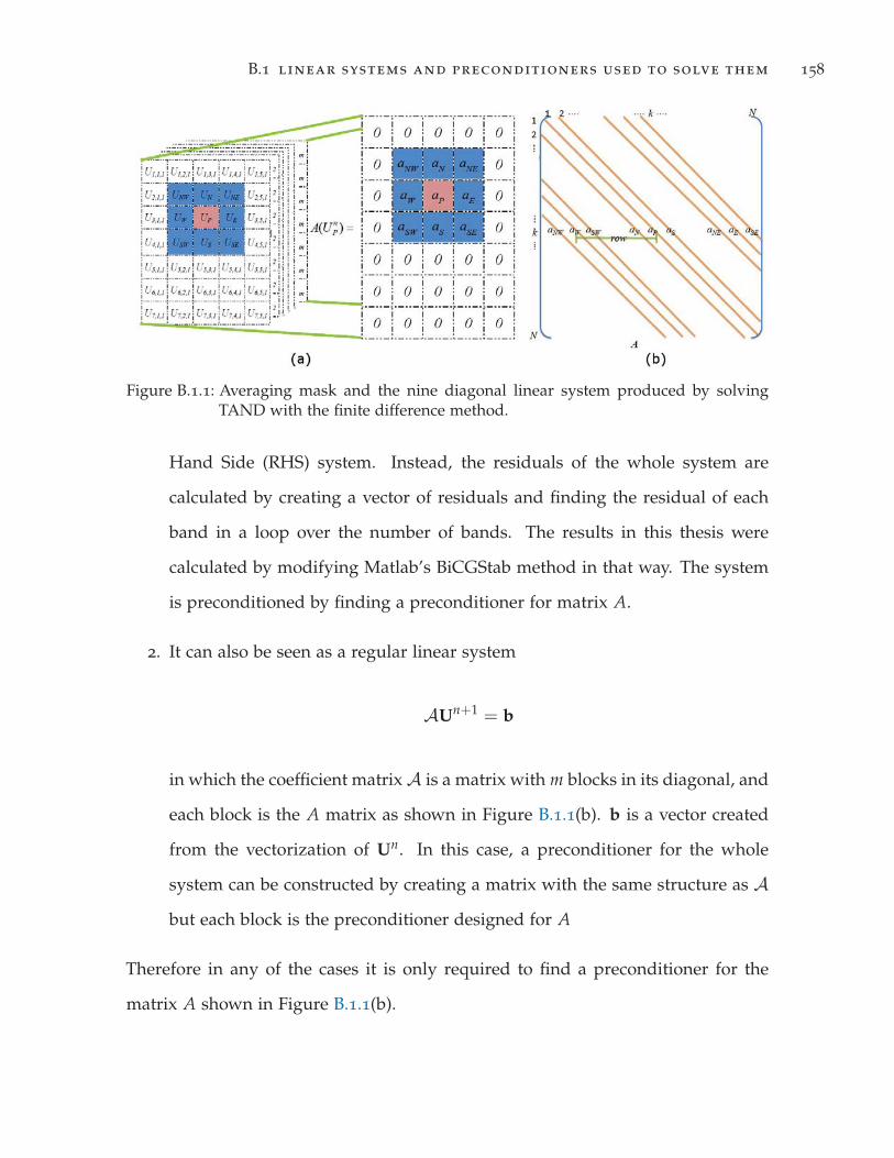
B.1 linear systems and preconditioners used to solve them 158
Figure B.1.1: Averaging mask and the nine diagonal linear system produced by solvingTAND with the finite difference method.
Hand Side (RHS) system. Instead, the residuals of the whole system are
calculated by creating a vector of residuals and finding the residual of each
band in a loop over the number of bands. The results in this thesis were
calculated by modifying Matlab’s BiCGStab method in that way. The system
is preconditioned by finding a preconditioner for matrix A.
2. It can also be seen as a regular linear system
AUn+1 = b
in which the coefficient matrix A is a matrix with m blocks in its diagonal, and
each block is the A matrix as shown in Figure B.1.1(b). b is a vector created
from the vectorization of Un. In this case, a preconditioner for the whole
system can be constructed by creating a matrix with the same structure as Abut each block is the preconditioner designed for A
Therefore in any of the cases it is only required to find a preconditioner for the
matrix A shown in Figure B.1.1(b).

B.2 peric preconditioner 159
Figure B.2.1: Schematic representation of the nine diagonal linear system resulting fromTAND.
b.2 peric preconditioner
Having a priory knowledge of the sparsity pattern of the coefficient matrix is an
advantage in order to design preconditioners based on the data. The preconditioner
presented in this section can be extended for any of the cases presented in Section
B.1.1. Let
Aφ = S (B.2.1)
be the linear system, where A is a nine diagonal matrix, φ is the vector of variables
and S is the RHS. The system is depicted in Figure B.2.1.
Since each row for the linear system only has nine values different from zero
then the system at row k is:
anwφnw + awφw + aswφsw + anφn + apφp
+asφs + anwφnw + aeφe + aseφse = Sp
(B.2.2)
Since the sparse pattern of matrix A is from a discretization from a regular grid, a
matrix C = L · U with the same diagonals as matrix A can be found. L and U have
nonzero coefficients on seven diagonals only, which coincide with the correspond-

B.2 peric preconditioner 160
Figure B.2.2: Schematic representation of the proposed matrices L, U and their productmatrix C
ing seven nonzero diagonals of A. The two diagonals left out correspond to two
opposite corner points aNE, aSW of the averaging mask shown in Figure B.1.1(a),
since the column major format is used to arrange φ. Otherwise they are aNW , aSE.
C with its decomposition is shown in Figure (B.2.1)
The following is the resulting coefficient of the LU product matrix, C, for a row
k:ck
nw =bknw;
ckw =bk
w + bknwbk−r−1
s ;
cksw =bk−r
s bkw;
ckn =bk
n + bk−r−1e bk
nw;
ckp =bk
p + bkre bk
w + bknbk−1
s + bknwbk−r−1
se ;
cks =bk
pbks + bkr
se bkw;
ckne =bk−1
e bkn;
cke =bk
e bkp + bk
nbk−1se ;
ckse =bk
pbkse;
(B.2.3)
For now on, the superscript k will be dropped and all the calculations will be
assumed to be at row k of the corresponding matrix, where r = n1.
B.2 peric preconditioner 161
Since L and U do not use φne and φsw, they can be approximated by using the
same bands used in their definition on the averaging mask and subtract them from
the center value, as follows:
φne ≈ α(φn + φe − φp
)(B.2.4)
φsw ≈ α(φs + φw − φp
)
Substituting Equations (B.2.4) in (B.2.2) and after some algebra :
(an + αane)φn + anwφnw + (ap − αane − αasw)φp + (as + αasw)φs
+aseφse + (aw + αasw)φw + (ae + αane)φe = Sp
(B.2.5)
is obtained. This equation produces a linear system
Aφ = S (B.2.6)
where the coefficient for the kth row is given by:
anw =anw
aw =aw + αasw
an =an + αane
ap =ap − αane − αasw
as =as + αasw
ae =ae + αane
ase =ase

B.2 peric preconditioner 162
Note that (B.2.6) only have seven diagonals and not nine as C = L · U. Assuming
that the equations (B.2.4) holds then
φne − α(φn + φe − φp
)= φsw − α
(φs + φw − φp
) ≈ 0 (B.2.7)
so the following system will be approximately equal to (B.2.6)
anwφnw + awφw + anφn + apφp + asφs + aeφe + aseφse
+csw[φsw − α
(φs + φw − φp
)]+ cnw
[φne − α
(φn + φe − φp
)]= Sp
(B.2.8)
Replacing the values of a’s in (B.2.8) and factoring for the φ’s, a linear system
is obtained. Then, making the corresponding φ’s coefficients in (B.2.8) equal to
corresponding C’s coefficients in (B.2.3), results in:
bnw =anw
bw =aw + αasw − bnwbk−r−1
s
αbk−rs + 1
bn =an + αane − bk−r−1
e bnw
αbk−1e + 1
bp =ap − bnbk−1s − bk−r
e bw − bnwbk−r−1se
+ α(bk−1e bn − asw − ane + bk−r
s bw)
bs =as + αasw − bk−r
se bw − αbk−rs bw
bp
be =ae + αane − bnbk−1
se − αbk−1e bn
bp
bse =ase
bp
which will be the coefficients of the diagonals in L and U in (B.2.3). The terms
without superscript are assumed at row k. All those calculations were done using
Matlab’s symbolic toolbox. This preconditioner was inspired by a method [103]

B.3 experimental results 163
Figure B.3.1: Comparison in terms of (a) total time, (b) relative residual and (c) number ofiterations that BiCGStab needs to converge after being preconditioned withILU(0), Jacobi diagonal and the proposed Peric Preconditioners. The linearsystem results from appliying TAND-EED to Indian Pines. (d) shows κ′1sentropy vs. number of iterations of TAND
proposed to solve the linear system in (B.2.1). But the coefficients for C result
from the approximation of (B.2.6), which in turn is the approximation to (B.2.1),
and does not inspire much reliability for a direct solver. But could be used as a
preconditioner. The results showed in the next section use α = 0.02.
b.3 experimental results
Figure B.3.1 shows the comparison of preconditioning BiCGStab using ILU(0), Ja-
cobi diagonal and the proposed Peric Preconditioners. Figure B.3.1(a) shows the

B.3 experimental results 164
total time for a preconditioned BiCGStab to obtain a solution. This time is ob-
tained after adding the time to create the preconditioner and solve the system. As
TAND-EED regularize the image the time needed to obtain a solution decrease in
all the preconditioners, except in Peric, in some intervals the Peric preconditioner
is slowing down the solution. From Figure B.3.1(a) is clear that the quickest pre-
conditioner is the ILU(0). Figure B.3.1(b) shows the results for the relative residual
error. BiCGStab was set to stop with a tolerance of 10−4.The different precondi-
tioned BiCGStabs produce a non monotone decreasing sequences of errors as the
number of iterations of TAND increases, except ILU that after TAND’s iteration 12,
its errors decrease. Figure B.3.1(c) shows the number of iterations that BiCGStab
needs to converge vs. the number of iterations of TAND. The shapes of the curves
for Figure B.3.1(a) and (c) are equal since the time need to solve the system is
proportional to the number of iterations that the preconditioned BiCGStab need
to converge. Figure B.3.1(d) shows κ′1s entropy, This value is almost identical for
each of the preconditioned BiCGStab in each iteration of TAND, showing that the
resulting images are very similar. κ′1s entropy was calculated

B I B L I O G R A P H Y
[1] H. Z. M. Shafri, A. Suhaili, and S. Mansor, “The performance of maximum
likelihood, spectral angle mapper, neural network and decision tree classi-
fiers in hyperspectral image analysis,” Journal of Computer Science, vol. 3, no. 6,
pp. 419–423, Jun. 2007.
[2] J. Weickert, Anisotropic Diffusion in Image Processing. Teubner-Verlag, 1998.
[3] D. Tschumperle and R. Deriche, “Diffusion PDEs on vector-valued images,”
IEEE Signal Processing Magazine, vol. 19, no. 5, pp. 16– 25, Sep. 2002.
[4] J. Martin – Herrero, “Anisotropic diffusion in the hypercube,” IEEE Trans-
actions on Geoscience and Remote Sensing, vol. 45, no. 5, pp. 1386–1398, May
2007.
[5] J. M. Duarte-Carvajalino, P. E. Castillo, and M. Velez-Reyes, “Comparative
study of Semi-Implicit schemes for nonlinear diffusion in hyperspectral im-
agery,” IEEE Transactions on Image Processing, vol. 16, no. 5, pp. 1303 –1314,
May 2007.
[6] J. Weickert, “Multiscale texture enhancement,” in Computer Analysis of Images
and Patterns, ser. Lecture Notes in Computer Science, V. Hlavác and R. Sára,
Eds. Springer Berlin / Heidelberg, 1995, vol. 970, pp. 230–237.
[7] T. Brox and J. Weickert, “Nonlinear matrix diffusion for optic flow estima-
tion,” in Proceedings of the 24th DAGM Symposium on Pattern Recognition. Lon-
don, UK: Springer-Verlag, 2002, pp. 446–453.
165

bibliography 166
[8] W. Fróstner and E. Gülch, “A fast operator for detection and
precise location of distinct points, corners and centers of circular
features,” in Proceedings of the ISPRS Intercommission Workshop on Fast
Processing of Photogrammetric Data, 1987, pp. 281–305. [Online]. Available:
http://www-cse.ucsd.edu/classes/sp02/cse252/foerstner/foerstner.pdf
[9] T. Lindeberg, Scale-Space Theory in Computer Vision, 1st ed. Springer, Dec.
1993.
[10] J. Bigün, G. H. Granlund, and J. Wiklund, “Multidimensional orientation es-
timation with applications to texture analysis and optical flow,” IEEE Trans-
actions on Pattern Analysis and Machine Intelligence, vol. 13, pp. 775–790, Aug.
1991.
[11] A. Rao and B. Schunck, “Computing oriented texture fields,” in CVGIP:
Graphical Models and Image Processing, vol. 53, San Diego, CA, USA, 1991, pp.
157–185.
[12] D. Tschumperlé, “PDE’s based regularization of multivalued images and
applications,” Ph.D. dissertation, Université de Nice-Sophia Antipolis, Dec.
2002.
[13] T. Preusser and M. Rumpf, “Anisotropic nonlinear diffusion in flow visual-
ization,” in Proceedings Visualization, Oct. 1999, pp. 325 –539.
[14] H. Scharr and H. Spies, “Accurate optical flow in noisy image sequences
using flow adapted anisotropic diffusion,” Signal Processing: Image Communi-
cation, vol. 20, no. 6, pp. 537 – 553, 2005, special Issue on Advanced Aspects
of Motion Estimation.
[15] B. Bouda, L. Masmoudi, and D. Aboutajdine, “CVVEFM: cubical voxels
and virtual electric field model for edge detection in color images,” Signal
bibliography 167
Processing, vol. 88, no. 4, pp. 905–915, Apr. 2008. [Online]. Available:
http://dx.doi.org/10.1016/j.sigpro.2007.10.006
[16] M. Lee and L. Bruce, “Applying cellular automata to hyperspectral edge
detection,” in IEEE International Geoscience and Remote Sensing Symposium
(IGARSS), Jul. 2010, pp. 2202 –2205.
[17] X. Chen and H. Chen, “A novel color edge detection algorithm in RGB color
space,” in IEEE 10th International Conference on Signal Processing (ICSP), Oct.
2010, pp. 793 –796.
[18] D. Tschumperlé and R. Deriche, “Vector-valued image regularization with
PDEs: a common framework for different applications,” IEEE Transactions on
Pattern Analysis and Machine Intelligence, vol. 27, no. 4, pp. 506–517, 2005.
[19] D. Tschumperlé, “Fast anisotropic smoothing of Multi-Valued images using
Curvature-Preserving PDE’s,” International Journal of Computer Vision, vol. 68,
pp. 65–82, 2006, 10.1007/s11263-006-5631-z.
[20] J. Weickert, “Coherence-Enhancing diffusion filtering,” International Journal of
Computer Vision, vol. 31, no. 2-3, pp. 111–127, 1999.
[21] J. Weickert and T. Brox, “Diffusion and regularization of vector- and matrix-
valued images,” Tech. Rep. preprint no. 58, Tech. Rep., 2002.
[22] H. Takeda, S. Farsiu, and P. Milanfar, “Kernel regression for image processing
and reconstruction,” IEEE Transactions on Image Processing, vol. 16, no. 2, pp.
349–366, Feb. 2007.
[23] J. Weickert, “Coherence-enhancing diffusion of colour images,” Image Vision
Comput., vol. 17, no. 3-4, pp. 201–212, 1999.

bibliography 168
[24] O. Drblíková, A. Handlovicová, and K. Mikula, “Error estimates of the finite
volume scheme for the nonlinear tensor-driven anisotropic diffusion,” Appl.
Numer. Math., vol. 59, no. 10, pp. 2548–2570, 2009.
[25] K. O. Riedel, “Corner-preserving anisotropic diffusion and junction detection
using the structure tensor,” in DAGM-Symposium, 1999, pp. 164–171.
[26] B. Burgeth, S. Didas, and J. Weickert, “A general structure tensor concept
and coherence-enhancing diffusion filtering for matrix fields,” Visualization
and Processing of Tensor Fields, pp. 305–323, 2009.
[27] J. R. Schott, Remote Sensing: The Image Chain Approach. Oxford University
Press, May 2007.
[28] R. A. Schowengerdt, Remote Sensing: Models And Methods for Image Processing.
Academic Press, Aug. 2006.
[29] D. Manolakis, D. Marden, and G. A. Shaw, “Hyperspectral image processing
for automatic target detection applications,” Lincoln Laboratory Journal, vol. 14,
no. 1, pp. 79–116, 2003.
[30] R. Resmini, Dimension Reduction of Hyperspectal Image (HSI) Data, Jul. 2005,
published: IPAM Graduate Summer School.
[31] U. o. C. S. Barbara, Hawaii’s Hyperspectral Remote Sensing as an Environmental
Monitoring Tool for Shallow Coral Reef Ecosystems. [Online]. Available:
http://emerald.ucsc.edu/hyperwww/hawaii.html
[32] H. Erives and G. J. Fitzgerald, “Automated registration of hyperspectral im-
ages for precision agriculture,” Comput. Electron. Agric., vol. 47, no. 2, pp.
103–119, 2005.

bibliography 169
[33] B. Datt, T. R. McVicar, T. G. Van Niel, D. L. Jupp, and J. S. Pearlman, “Prepro-
cessing EO-1 hyperion hyperspectral data to support the application of agri-
cultural indexes,” IEEE Transactions on Geoscience and Remote Sensing, vol. 41,
no. 6, pp. 1246–1259, 2003.
[34] D. G. Ferris, R. A. Lawhead, E. D. Dickman, N. Holtzapple, J. A. Miller, S. Gro-
gan, S. Bambot, A. Agrawal, and M. L. Faupel, “Multimodal hyperspectral
imaging for the noninvasive diagnosis of cervical neoplasia,” Journal of Lower
Genital Tract Disease, vol. 5, no. 2, pp. 65–72, 2001.
[35] Z. Liu, Q. Li, J. Yan, and Q. Tang, “A novel hyperspectral medical sensor for
tongue diagnosis,” Sensor Review, vol. 27, no. 1, pp. 57–60, 2007.
[36] K. M. Rajpoot, N. M. Rajpoot, and M. Turner, “Hyperspectral colon tissue
cell classification,” SPIE Medical Imaging (MI), 2004.
[37] S. J. Hamilton and R. A. Lodder, “Hyperspectral imaging technology for phar-
maceutical analysis,” in Proc Soc Photo-Optic Instrum Eng, 2002, pp. 2002–4626.
[38] D. B. Malkoff and W. R. Oliver, “Hyperspectral imaging applied to forensic
medicine,” in Proceedings of SPIE, vol. 3920, 2000, p. 108.
[39] A. A. Gowen, C. P. O’Donnell, P. J. Cullen, G. Downey, and J. M. Frias, “Hy-
perspectral imaging-an emerging process analytical tool for food quality and
safety control,” Trends in Food Science & Technology, vol. 18, no. 12, pp. 590–598,
2007.
[40] J. M. Duarte-Carvajalino, G. Sapiro, M. Velez-Reyes, and P. E. Castillo, “Mul-
tiscale representation and segmentation of hyperspectral imagery using geo-
metric partial differential equations and algebraic multigrid methods,” IEEE
Transactions on Geoscience and Remote Sensing, vol. 46, no. 8, pp. 2418 –2434,
Aug. 2008.

bibliography 170
[41] R. M. Cavalli, F. Colosi, A. Palombo, S. Pignatti, and M. Poscolieri, “Remote
hyperspectral imagery as a support to archaeological prospection,” Journal of
Cultural Heritage, vol. 8, no. 3, pp. 272–283, 2007.
[42] R. C. González and R. E. Woods, Digital image processing, 3rd ed. Prentice
Hall, 2007.
[43] H. Ren and C. I. Chang, “Automatic spectral target recognition in hyperspec-
tral imagery,” Aerospace and Electronic Systems, IEEE Transactions on, vol. 39,
no. 4, pp. 1232–1249, 2004.
[44] C. Bazán, M. Miller, and P. Blomgren, “Structure enhancement diffusion
and contour extraction for electron tomography of mitochondria,”
Journal of Structural Biology, vol. 166, no. 2, pp. 144–155, May
2009. [Online]. Available: http://www.sciencedirect.com/science/article/
B6WM5-4VR246P-1/2/7941e8ba9aa4e71fdd5038c422fbb9f0
[45] J. Weickert, B. M. Romeny, and M. A. Viergever, “Efficient and reliable
schemes for nonlinear diffusion filtering,” IEEE Transactions on Image Process-
ing, vol. 7, no. 3, pp. 398 –410, Mar. 1998.
[46] J. Weickert, “Nonlinear diffusion filtering,” in Handbook on Computer Vision
and Applications: Signal Processing and Pattern Recognition. Academic Press,
1999, vol. 2, pp. 423–450.
[47] L. J. Grady and J. R. Polimeni, Discrete Calculus: Applied Analysis on Graphs for
Computational Science. Springer, Aug. 2010.
[48] L. Florac, Image Structure, ser. Computational Imaging and Vision, 1997,
vol. 10. [Online]. Available: http://www.springer.com/computer/image+
processing/book/978-0-7923-4808-5
bibliography 171
[49] T. G. Kolda and B. W. Bader, “Tensor decompositions and applications,”
SIAM REVIEW, vol. 51, no. 3, pp. 455–500, 2009.
[50] S. Aja-Fernández, R. d. L. Garcia, D. Tao, and X. Li, Tensors in Image Processing
and Computer Vision, 1st ed. Springer, Jul. 2009.
[51] J. Bigün and G. H. Granlund, “Optimal orientation detection of linear symme-
try,” in IEEE First International Conference on Computer Vision, London, Great
Britain, Jun. 1987, pp. 433–438.
[52] Wikipedia contributors, “Structure tensor,” May 2012, page Version ID:
490314716. [Online]. Available: http://en.wikipedia.org/w/index.php?title=
Structure_tensor&oldid=490314716
[53] M. Nicolescu and G. Medioni, “Motion segmentation with accurate
boundaries: a tensor voting approach,” in Proceedings of the 2003 IEEE
computer society conference on Computer vision and pattern recognition, ser.
CVPR’03. Washington, DC, USA: IEEE Computer Society, 2003, pp. 382–389.
[Online]. Available: http://dl.acm.org/citation.cfm?id=1965841.1965890
[54] J. Wiklund, V. Nicolas, P. Rondao, M. Andersson, and H. Knutsson, “T-flash:
Tensor visualization in medical studio,” Tensors in Image Processing and Com-
puter Vision, pp. 455–466, 2009.
[55] G. Kindlmann, “Superquadric tensor glyphs,” in Proceedings of IEEE
TVCG/EG Symposium on Visualization, vol. 2004, 2004, pp. 147–154.
[56] A. Brun and H. Knutsson, “Tensor glyph warping: Visualizing metric ten-
sor fields using riemannian exponential maps,” Visualization and Processing of
Tensor Fields, pp. 139–160, 2009.

bibliography 172
[57] L. Cammoun, C. Castaño-Moraga, E. Muñoz-Moreno, D. Sosa-Cabrera,
B. Acar, M. Rodriguez-Florido, A. Brun, H. Knutsson, and J. P. Thiran, “A
review of tensors and tensor signal processing,” in Tensors in Image Processing
and Computer Vision, ser. Advances in Pattern Recognition, S. Aja-Fernández,
R. Luis García, D. Tao, and X. Li, Eds. Springer London, 2009, pp. 1–32.
[58] B. Jähne, “Local structure,” in Handbook of Computer Vision and Applications,
ser. Signal Processing and Pattern Recognition. Academic Press, 1999, vol. 2,
pp. 209–238.
[59] G. H. Granlund and H. Knutsson, Signal processing for computer vision.
Springer, 1995.
[60] M. Kass and A. Witkin, “Analyzing oriented patterns,” Comput. Vision Graph.
Image Process., vol. 37, no. 3, pp. 362–385, Mar. 1987.
[61] H. Knutsson, “Representing local structure using tensors,” in The 6th Scan-
dinavian Conference on Image Analysis, Oulu, Finland, June 1989, pp. 244–251,
report LiTH–ISY–I–1019, Computer Vision Laboratory, Linköping University,
Sweden, 1989.
[62] H. Knutsson, C.-F. Westin, and M. Andersson, “Representing local structure
using tensors ii,” in Proceedings of the 17th Scandinavian conference on Image
analysis, ser. SCIA-11. Berlin, Heidelberg: Springer-Verlag, 2011, pp. 545–
556.
[63] H. Knutsson and M. Andersson, “What’s so good about quadrature filters?”
in Proceedings of the International Conference on Image Processing, vol. 3, Sep.
2003, pp. III – 61–4 vol.2.
[64] B. Rieger and L. J. V. Vliet, “A systematic approach to nD orientation repre-
sentation,” Image Vis. Comput, vol. 22, pp. 453–459, 2004.

bibliography 173
[65] v. d. R. Boomgaard and v. d. J. Weijer, “Robust estimation of
orientation for texture analysis,” in The 2nd international workshop on
texture analysis and synthesis, 2002, pp. 135–138. [Online]. Available:
http://dare.uva.nl/record/104550
[66] T. Brox, R. Boomgaard, F. Lauze, J. Weijer, J. Weickert, P. Mrázek,
and P. Kornprobst, “Adaptive structure tensors and their applications,”
in Visualization and Processing of Tensor Fields, ser. Mathematics and
Visualization, J. Weickert and H. Hagen, Eds. Springer Berlin Heidelberg,
2006, pp. 17–47, 10.1007/3-540-31272-2_2. [Online]. Available: http:
//dx.doi.org/10.1007/3-540-31272-2_2
[67] S. Di Zenzo, “A note on the gradient of a multi-image,” Computer Vision,
Graphics, and Image Processing, vol. 33, no. 1, pp. 116 – 125, 1986.
[68] G. Aubert and P. Kornprobst, Mathematical problems in image processing: partial
differential equations and the calculus of variations. Springer-Verlag New York
Inc, 2006.
[69] J. H. Ferziger and M. Peric, Computational methods for fluid dynamics. Springer
Berlin, 1999.
[70] J. Weickert, “A review of nonlinear diffusion filtering,” Scale-space theory in
computer vision, pp. 1–28, 1997.
[71] ——, “Scale-Space properties of nonlinear diffusion filtering with a diffusion
tensor,” Laboratory of Technomathematics, University of Kaiserslautern, P.O,
Tech. Rep., 1994.
[72] F. Catte, P. L. Lions, J. M. Morel, and T. Coll, “Image selective smoothing and
edge detection by nonlinear diffusion,” SIAM J. Numer. Anal., vol. 29, no. 1,
pp. 182–193, 1992.

bibliography 174
[73] P. Perona and J. Malik, “Scale-space and edge detection using anisotropic dif-
fusion,” IEEE Transactions on Pattern Analysis and Machine Intelligence, vol. 12,
no. 7, pp. 629 –639, Jul. 1990.
[74] L. Alvarez, F. Guichard, P. L. Lions, and J. M. Morel, “Axioms and fundamen-
tal equations of image processing,” Archive for Rational Mechanics and Analysis,
vol. 123, no. 3, pp. 199–257, 1993.
[75] M. Z. Nashed and O. Scherzer, “Least squares and bounded variation regu-
larization with nondifferentiable functionals,” Numerical Functional Analysis
and Optimization, vol. 19, no. 7, pp. 873–901, 1998.
[76] G. H. Cottet and L. Germain, “Image processing through reaction combined
with nonlinear diffusion,” Mathematics of Computation, vol. 61, no. 204, pp.
659–673, 1993.
[77] O. Drblíková and K. Mikula, “Convergence analysis of finite volume scheme
for nonlinear tensor anisotropic diffusion in image processing,” SIAM J. Nu-
mer. Anal., vol. 46, no. 1, pp. 37–60, 2007.
[78] C. Monet, “Woman with a parasol, looking left,” 1886, published: Musée
d’Orsay, Paris.
[79] R. Brügelmann and W. Förstner, “Noise estimation for color edge extraction,”
in Robust Computer Vision, W. Förstner and S. Ruwiedel, Eds. Wichmann,
Karlsruhe, 1992, pp. 90–107.
[80] S. Nath and K. Palaniappan, “Adaptive robust structure tensors for orienta-
tion estimation and image segmentation,” in Advances in Visual Computing,
ser. Lecture Notes in Computer Science, G. Bebis, R. Boyle, D. Koracin, and
B. Parvin, Eds. Springer Berlin / Heidelberg, 2005, vol. 3804, pp. 445–453,
10.1007/11595755_54.

bibliography 175
[81] P. Mrazek, J. Weickert, and A. Bruhn, “On robust estimation and smoothing
with spatial and tonal kernels,” in Geometric Properties for Incomplete data,
R. Klette, R. Kozera, L. Noakes, and J. Weickert, Eds. Dordrecht: Kluwer
Academic Publishers, 2006, vol. 31, pp. 335–352. [Online]. Available: http:
//www.springerlink.com/content/g552624mnkrr2306/export-citation/
[82] T. Brox, J. Weickert, B. Burgeth, and P. Mrazek, “Nonlinear structure tensors,”
Image and Vision Computing, vol. 24, no. 1, pp. 41–55, Jan. 2006. [Online].
Available: http://dl.acm.org/citation.cfm?id=1709276
[83] M. Marin-McGee and M. Velez-Reyes, “A structure tensor for hyperspectral
images,” in 3rd Workshop on Hyperspectral Image and Signal Processing: Evolu-
tion in Remote Sensing (WHISPERS). IEEE, Jun. 2011, pp. 1–4.
[84] R. Kimmel, R. Malladi, and N. Sochen, “Image processing via the beltrami
operator,” in In Proc. of 3-rd Asian Conf. on Computer Vision, Hong Kong, 1998,
pp. 574–581.
[85] P. Bakker, L. J. van Vliet, and P. W. Verbeek, “Edge preserving orientation
adaptive filtering,” in IEEE Computer Society Conference on Computer Vision
and Pattern Recognition, vol. 1. IEEE, 1999, p. 540 Vol. 1.
[86] R. v. d. Boomgaard, Decomposition of the Kuwahara-Nagao Operator in Terms of
a Linear Smoothing and a Morphological Sharpening, R. B. H. Talbot, Ed., 2002.
[87] M. Kuwahara, K. Hachimura, S. Eiho, and M. Kinoshita, Processing of RI-
angiocardiographic images, J. K. Preston and M. Onoe, Eds. Plenum Press,
1976.
[88] M. Nagao and T. Matsuyama, “Edge preserving smoothing,” Computer Graph-
ics and Image Processing, vol. 9, no. 4, pp. 394–407, Apr. 1979.
bibliography 176
[89] W. Wang, J. Gao, and K. Li, “Structure-Adaptive anisotropic filter with local
structure tensors,” in Second International Symposium on Intelligent Information
Technology Application, IITA ’08., vol. 2, Dec. 2008, pp. 1005 –1010.
[90] M. Middendorf and H. Nagel, “Empirically convergent adaptive estimation
of grayvalue structure tensors,” in Pattern Recognition, L. Gool, Ed. Berlin,
Heidelberg: Springer Berlin Heidelberg, 2002, vol. 2449, pp. 66–74. [Online].
Available: http://www.springerlink.com/content/fbbrynkyy8yhfd4q/
[91] H. H. Nagel and A. Gehrke, “Spatiotemporally adaptive estimation and
segmentation of OF-fields,” in Computer Vision ECCV-98, H. Burkhardt and
B. Neumann, Eds. Berlin/Heidelberg: Springer-Verlag, vol. 1407, pp. 86–102.
[92] G. Z. Yang, P. Burger, D. N. Firmin, S. R. Underwood, and D. B. Longmore,
“Structure adaptive anisotropic filtering,” in Fifth International Conference on
Image Processing and its Applications, Jul. 1995, pp. 717 –721.
[93] A. Grigor’yan, “Heat kernels on weighted manifolds and applications,” The
ubiquitous heat kernel: AMS special session, the ubiquitous heat kernel, October 2-4,
2003, Boulder, Colorado, vol. 398, p. 93, 2006.
[94] M. Ovsjanikov, Q. Mérigot, F. Mémoli, and L. Guibas, “One point isometric
matching with the heat kernel,” Computer Graphics Forum, vol. 29, no. 5, pp.
1555–1564, 2010.
[95] S. Rosenberg, The Laplacian on a Riemannian Manifold: An Introduction to Anal-
ysis on Manifolds. Cambridge University Press, Jan. 1997.
[96] P. Auscher, T. Coulhon, and A. Grigor’yan, Heat kernels and analysis on man-
ifolds, graphs, and metric spaces: lecture notes from a quarter program on heat
kernels, random walks, and analysis on manifolds and graphs : April 16-July 13,

bibliography 177
2002, Emile Borel Centre of the Henri Poincaré Institute, Paris, France. American
Mathematical Soc., 2003.
[97] V. Van Gogh, “Road with cypress and star,” 1890, published: Auvers-sur-
Oise.
[98] C. Shannon, “A mathematical theory of communication,” Bell system technical
journal, vol. 27, 1948.
[99] Jet Propulsion Laboratory, NASA, “AVIRIS line of deep hori-
zon gulf of mexico oil spill. flight ID =f100517t01 and runId=
p00_r06,” http://aviris.jpl.nasa.gov/ql/10qlook/f100517t01p00r06_geo.jpeg,
2010. [Online]. Available: http://aviris.jpl.nasa.gov/ql/10qlook/
f100517t01p00r06_geo.jpeg
[100] M. Marin-McGee and M. Velez-Reyes, “Enhancement of flow-like structures
in hyperspectral imagery using tensor nonlinear anisotropic diffusion,” in
Proc. SPIE 8048, 2011, pp. 80 480E–80 480E–9.
[101] J. C. Strikwerda, Finite difference schemes and partial differential equations. Soci-
ety for Industrial Mathematics, 2004.
[102] Y. Saad, Iterative Methods for Sparse Linear Systems, Second Edition, 2nd ed.
Society for Industrial and Applied Mathematics, Apr. 2003.
[103] M. Peric, “Efficient semi-implicit solving algorithm for nine-diagonal coeffi-
cient matrix,” Numerical Heat Transfer, vol. 11, no. 3, pp. 251–279, 1987.
[104] R. N. Clark, G. A. Swayze, K. E. Livo, R. F. Kokaly, S. J. Sutley, J. B. Dalton,
R. R. McDougal, and C. A. Gent, “Imaging spectroscopy: Earth and planetary
remote sensing with the USGS tetracorder and expert systems,” Journal of
Geophysical Research, vol. 108, no. E12, p. 5131, 2003.

bibliography 178
[105] Purdue Research Foundation, “MultiSpec | tutorials,”
https://engineering.purdue.edu/~biehl/MultiSpec/hyperspectral.html,
2012. [Online]. Available: https://engineering.purdue.edu/~biehl/
MultiSpec/hyperspectral.html
[106] J. Kerekes, A. Cisz, and R. Simmons, “A comparative evaluation of spec-
tral quality metrics for hyperspectral imagery,” Proceedings of Algorithms and
Technologies for Multispectral, Hyperspectral, and Ultraspectral Imagery XI, pp.
469–480, 2005.
[107] J. J. Cipar, “Background spectral library for fort A.P. hill, virginia,” vol. 5544.
SPIE, 2004, pp. 35–46.
[108] J. J. Fernández and S. Li, “An improved algorithm for anisotropic nonlinear
diffusion for denoising cryo-tomograms,” Journal of Structural Biology, vol.
144, no. 1-2, pp. 152–161, 2003.
[109] P. Mrázek and M. Navara, “Selection of optimal stopping time for nonlinear
diffusion filtering,” Int. J. Comput. Vision, vol. 52, no. 2-3, pp. 189–203, May
2003. [Online]. Available: http://dl.acm.org/citation.cfm?id=641431.641463
[110] J. B. Campbell and R. H. Wynne, Introduction to Remote Sensing, 5th ed. Guil-
ford Press, Jun. 2011.
[111] E. T. Slonecker, D. M. Shaw, and T. M. Lillesand, “Emerging legal and ethical
issues in advanced remote sensing technology,” Photogrammetric engineering
and remote sensing, vol. 64, no. 6, pp. 589–595, 1998. [Online]. Available:
http://cat.inist.fr/?aModele=afficheN&cpsidt=2241832
[112] N. Rastogi, “Google’s blind spots,” Slate, Dec. 2008. [Online]. Avail-
able: http://www.slate.com/articles/news_and_politics/explainer/2008/
12/googles_blind_spots.html

bibliography 179
[113] S. Hitchings, “Policy assessment of the impacts of remote-sensing technol-
ogy,” Space Policy, vol. 19, no. 2, pp. 119–125, May 2003. [Online]. Available:
http://library.uprm.edu:2051/science/article/pii/S0265964603000171
[114] United Nations, “Declaration of principles regarding the remote sensing of
earth from space.” 1987.
[115] “Camp delta, google earth and the ethics of remote sensing in archaeology,”
vol. 42. [Online]. Available: http://www.tandfonline.com/doi/abs/10.1080/
00438243.2010.498640
[116] S. McKee, “Remote sensing issues at the supreme court of canada,”
BULLETIN-ASSOCIATION OF CANADIAN MAP LIBRARIES AND
ARCHIVES, vol. 123, p. 3, 2005.
[117] “Satellite evidence of human rights violations (1): Darfur and zimbabwe,”
http://filipspagnoli.wordpress.com/2009/01/31/satellite-evidence-of-
human-rights-violations/, Jan. 2009. [Online]. Available: http://filipspagnoli.
wordpress.com/2009/01/31/satellite-evidence-of-human-rights-violations/
[118] American Association for the Advancement of Science, “AAAS - geospatial
technologies and human rights,” http://shr.aaas.org/geotech/index.shtml.
[Online]. Available: http://shr.aaas.org/geotech/index.shtml
[119] “Satellite sentinel project,” http://www.satsentinel.org/. [Online]. Available:
http://www.satsentinel.org/
[120] Rhett Butler, “Satellites and google earth prove potent con-
servation tool by rhett butler: Yale environment 360,”
http://e360.yale.edu/content/feature.msp?id=2134, Mar. 2009. [Online].
Available: http://e360.yale.edu/content/feature.msp?id=2134

bibliography 180
[121] G. Steidl and T. Teuber, “Diffusion tensors for processing sheared and rotated
rectangles,” Image Processing, IEEE Transactions on, vol. 18, no. 12, pp. 2640 –
2648, dec. 2009.
[122] G. Gravvanis, C. Filelis-Papadopoulos, and K. Giannoutakis, “Solving finite
difference linear systems on GPUs: CUDA based parallel explicit precondi-
tioned biconjugate conjugate gradient type methods,” The Journal of Supercom-
puting, pp. 1–15.
[123] R. Mendez-Rial, M. Calvino-Cancela, and J. Martin-Herrero, “Accurate im-
plementation of anisotropic diffusion in the hypercube,” IEEE Geoscience and
Remote Sensing Letters, vol. 7, no. 4, pp. 870–874, Oct. 2010.
[124] R. Mendez-Rial and J. Martin-Herrero, “Efficiency of Semi-Implicit schemes
for anisotropic diffusion in the hypercube,” IEEE Transactions on Image Pro-
cessing, 2011.