~ 1 ~

The force on a cylindrical steel slug inside a finite solenoid

We will look at a cylindrical air-core solenoid with height , inside radius , of closely-

spaced wire per layer, in the winding and wound with wire having an outside diameter .

The following figure shows the co-ordinate frame we will use, with origin at the geometric center of

the coil. The -axis is coincident with the coil’s centerline and is pointed in the positive direction

determined by applying the right-hand rule to the current flowing in the winding.

is the thickness of the winding, which consists of layers wound with wire having an

outside diameter of . The height of the coil and the number of turns per layer are similarly related

by . Point is the center of the face established by the topmost turn(s). I have

shown an -axis perpendicular to the -axis. There will also be a -axis, perpendicular to both of these

axes. In due course, we will take advantage of the fact that the solenoid is rotationally symmetric around

its longitudinal axis, and simplify the analysis by looking at a typical -axis, which we will refer to as the

-axis.

We have examined this arrangement before, in the paper titled The magnetic field in and around a finite

cylindrical air-core solenoid. In that paper, I described how to calculate the magnetic field intensity

everywhere inside and outside the solenoid, except inside the winding itself. In addition, that paper

described a numerical method for numerically approximating the magnetic field intensity anywhere in a

rectangular region lying in any plane containing the longitudinal axis.

The purpose of this paper is to calculate the force this solenoid exerts on a cylindrical steel slug placed

inside. As an additional restriction, we will align the longitudinal axis of the slug with the longitudinal

axis of the solenoid. We will describe the slug by its radius , its length (or height, to be consistent

with the notation used for the solenoid) and its relative permeability . Obviously, the slug

must made from some magnetic material or it will not respond to the solenoid’s magnetic field at all. In

addition, the slug’s radius must be a little less than the solenoid’s inner radius or it will not fit

inside.

Let us define a parameter as the -co-ordinate of the geometric center of the slug with respect to the

origin . This will establish the slug’s displacement along the centerline of the solenoid. Because the

slug and the solenoid are rotationally symmetric, we only need one parameter to describe their relative

positions. The following figure shows the configuration we will examine.

-axis

-axis

current

Current

~ 2 ~

-axis

-axis

We will want to understand how the force depends on the slug’s three physical parameters: ,

and . In addition, we will want to understand how the force depends on the slug’s axial position

. The range of s which we will examine is bounded on the right by , with the slug’s

center at the solenoid’s center. But, it is premature to set an end point on the left. How far we choose to

look to the left depends on how quickly the force decreases once the slug passes through face .

We will make the following assumptions:

The guiderails which constrain the slug to the centerline are ignored. This is a good assumption if

the guiderails are non-magnetic.

The -axis is horizontal, so the effect of gravity can be ignored.

In the earlier paper, we developed the equations by which we can calculate the axial component and

radial component of the magnetic field intensity generated by the solenoid at any point . Because

the magnetic field of the solenoid is radially symmetric, there is no third component of the magnetic field.

The two equations are:

These two expressions assume that the solenoid is in free space, or air. If the point in question is

occupied by some material whose permeability is not equal to , then these equations do not apply.

What we need to do is to determine what the expressions for and are when there is some material at

point . So, let us consider a point which is inside the slug. What happens when current flows

through the turns in the surrounding solenoid and sets up a magnetic field at and around this point? We

can describe the response in two parts.

Firstly, the solenoid’s magnetic field is augmented, or “amplified”. In response to the external magnetic

field, free electrons in the metal begin to move in small circles. Within small volumes, called domains,

the electrons’ circles are oriented in a common direction. Their aggregate circular motion generates a

magnetic field – the so-called induced field. A material in which the electrons are so tightly bound to

their mother atoms that they cannot respond to an external magnetic field, such as wood or air, does not

produce an induced field. A material in which there are “free” electrons, but such that the free electrons’

small circles are not organized on a macroscopic scale, such as aluminum, does not produce an induced

field either.

I should mention that the orbiting of electrons is not the only component of the circular motion of charge.

The electrons also spin. The direction of the spin axis is also affected by the external field, and becomes

~ 3 ~

more closely aligned to the direction of the external magnetic field as the latter increases in strength. In

many cases, the contribution of spin to the induced field is comparable to or greater than that of the orbits.

In any event, the orbiting and spin-axis aligning of the electrons at and around point generates a

small magnetic field. Similar motion occurs at all points within the slug. The total magnetic field which

exists at point is therefore the sum of the external field of the solenoid plus all of the small magnetic

fields generated by electronic motion at all of the points within the slug. The total magnetic field can be

hundreds or thousands of times greater than that of the external field alone. The degree of augmentation

is measured by the relative permeability . This is a macroscopic property of a magnetic material. It is a

dimensionless number which multiplies the permeability of free space.

Suppose that the magnetic field generated by the solenoid at point is given by when the

solenoid is empty or, rather, filled with air. If a piece of magnetic material is placed in the solenoid such

that point is within the piece, then the total magnetic field at point will be equal to

.

This is a great convenience to us. All we have to do to calculate the magnetic field within the slug is to

multiply the solenoid’s “empty” field by a constant. The existence of magnetic material at any point

increases the strength of the magnetic field at that point but does not change its direction or the relative

magnitude of its components.

Now, let us look at the second part of the response. Any charged particle will experience a force if it is

placed in an electric field. Any charged particle which is moving will experience a force if it is placed in

a magnetic field. The material which makes up our slug is composed of a huge number of charged

particles. There are the free electrons, whose motion in small circles has already been mentioned. There

are the protons in all the nuclei of all the atoms in the metal. There are the quarks inside the neutrons in

the nuclei although, as a whole, the neutrons are electrically neutral. There are the electrons orbiting

those nuclei which are too tightly bound to respond independently to the magnetic field. In fact, all of

these other charged particles hugely outnumber the free electrons. All of the charged particles, not just

the free electrons, will experience a force from an electric field (if there is one) and from a magnetic field

(if there is one and if the charged particles are moving).

Fortunately, in this study, we can ignore the protons, the neutrons and the bound electrons. We can

ignore them because the forces exerted on them by the external electric and magnetic fields do not cause a

net force on the slug. By a “net” force, we mean a force which would move the slug as a rigid body. The

protons, neutrons and the bound electrons constitute atoms, or ions if they have contributed a free electron

or two. They are bound together by a host of inter-atomic electromagnetic forces which hold them in

place. They constitute the framework of the metal. Unless the external fields are so great that they tear

the metal apart, by melting, for example, the atoms and ions will retain their places in the matrix. The

external fields will cause stresses inside the matrix, which under some circumstances and configurations

can tend to separate the atoms and ions, but they do not give rise to a net force on the material as a rigid

body.

Furthermore, if the material is electrically neutral as a whole, then an external electric field will not

produce any net force on the body. It would cause internal stresses, but not a net external force.

For these reasons, we can confine our attention to the free electrons. They can be subject to a force which

has both an electrostatic component (the electromotive force) and a magnetostatic component (the

magnetomotive force). It was Messr. Lorentz who gave the first rigorous treatment of this force. The

Lorentz force, as it is called, acting on a single charged particle with charge is equal to:

~ 4 ~

This is the instantaneous force acting on the charged particle. The electrostatic force is proportional to the

charge and to the strength of the electrostatic field and acts in the direction of the electrostatic field .

The magnetomotive force is proportional to the charge and to the strength of the magnetostatic field

. It is also proportional to the speed of the charged particle. If the charged particle is stationary

relative to the magnetic field, then there will be no magnetomotive force on it.

The direction of the magnetomotive force is also special. The multiplication in Equation is a vector

cross-product. is a third vector, which is perpendicular to both the velocity and the

magnetostatic field . This means that the magnetomotive force will act at right angles to the

charged particle’s direction of travel. A force which acts at right angles is what leads to circular motion.

Equation gives the non-relativistic version of the Lorentz force. If the charged particle moves at a

speed which is an appreciable fraction of the speed of light, then delays need to be introduced into the

expression, so that the charged particle responds to conditions the correct light-speed in the past.

I have taken care to subscript the electrostatic and magnetostatic fields as and . They are

“total” fields, not to be confused with what may be the “external” fields in a particular situation. If there

was only one charged particle in the situation, then the two sets of fields would be the same. If there are

two or more charged particles, though, the movement of either one will affect the other. If there is a huge

number of charged particles, as there is in our slug, then the movement of all of them affects the fields

acting on all of them, in a recursive but instantaneous way.

Equation can be used directly in some situations, if there are very few charged particles or if the

velocities of the charged particles are known or constrained in some way. For example, if the charged

particles are constrained to move along a thin wire, Equation can be expressed in terms of the

geometry of the wire in a helpful way. But, if there are a lot of charged particles which are free to move

in three dimensions, as is the case in a plasma or a metal, Equation is of little use. All is not lost,

though, because it is possible to generalize the Lorentz equation so that it applies to a macroscopic three-

dimensional region. The word macroscopic is key. Whereas Equation describes a single charged

particle by its charge and velocity , the generalized Lorentz force describes a large number of charged

particles by their statistical properties, charge density and current density. These are densities per unit

volume. They apply to little bits of volume, but not bits of volume that are so small that the statistical

properties lose their meaning. The generalization is done by using Maxwell’s equations, which also treat

charged particles using their statistical, macroscopic, properties.

I have already done the generalization and described it in the paper titled Generalizing the Lorentz force

to a region containing charge. In its generalized form, the Lorentz equation can be written as:

This is the force per unit volume on the free electrons in the slug. The force acting on any small bit of

volume is expressed as a function of the total electric field and total magnetic field which exist in and

around the small bit of volume.

~ 5 ~

Equation is a very general result. It accounts for all aspects of sub-warp electromagnetism. It can

handle time-varying and non-uniform electric and magnetic fields. It is independent of co-ordinate

system. Furthermore, it does not include any of those nasty curls.

Units are defined in the SI system so that the permittivity and permeability of free space,

respectively, have a product equal to the reciprocal of the square of the speed of light. The

permeability of free space is equal to [Henries per meter]. Since the Henry is a

derived unit, the unit of permeability can also be expressed as [Newtons per Ampere squared] and

in other forms as well.

In the present application, with the slug inside the solenoid, the electric field is not important and the

terms in Equation which refer to the electric field can be removed. In addition, we have already

seen that the total magnetic field at any point inside the slug is a multiple of the magnetic field

generated by the empty solenoid at that point. Therefore, the expression for can be simplified in our

case to:

The constant is not affected by any of the spatial derivatives and can be withdrawn to leave:

Now, the spatial derivatives grad and div can be awkward to deal with. I feel most comfortable

working with them in Cartesian co-ordinates. Let us assume that we have some way of expressing

in terms of its components in a Cartesian co-ordinate frame, thus:

Then, the divergence is given by (dropping the subscript to avoid too much clutter):

The quantity is then simply the scalar multiplied by the vector :

The dot-product is also a scalar, but it is an operator, which takes certain spatial derivatives of

the quantities upon which it acts. can be expanded as:

~ 6 ~

In Equation , the operator takes the spatial derivatives of the coil’s magnetic field . The

result is:

Adding the two vectors gives:

Now, the third and last term in the expression for the force per unit volume is a gradient:

Substituting the appropriate terms into Equation gives the force per unit volume as:

Now is a good time to deal with the some of the symmetries which exist in our configuration. If we are

looking at some particular point inside the slug, we can without any loss of generality pick the -axis in

the figures above so that the point of interest lies in the - plane. Because the magnetic field generated

by the coil is radial, the transverse component is zero at all points in the - plane. It follows that all

derivatives with respect to are also zero. Removing all the zero terms leaves:

Then, we can use the product rule to re-write this as:

~ 7 ~

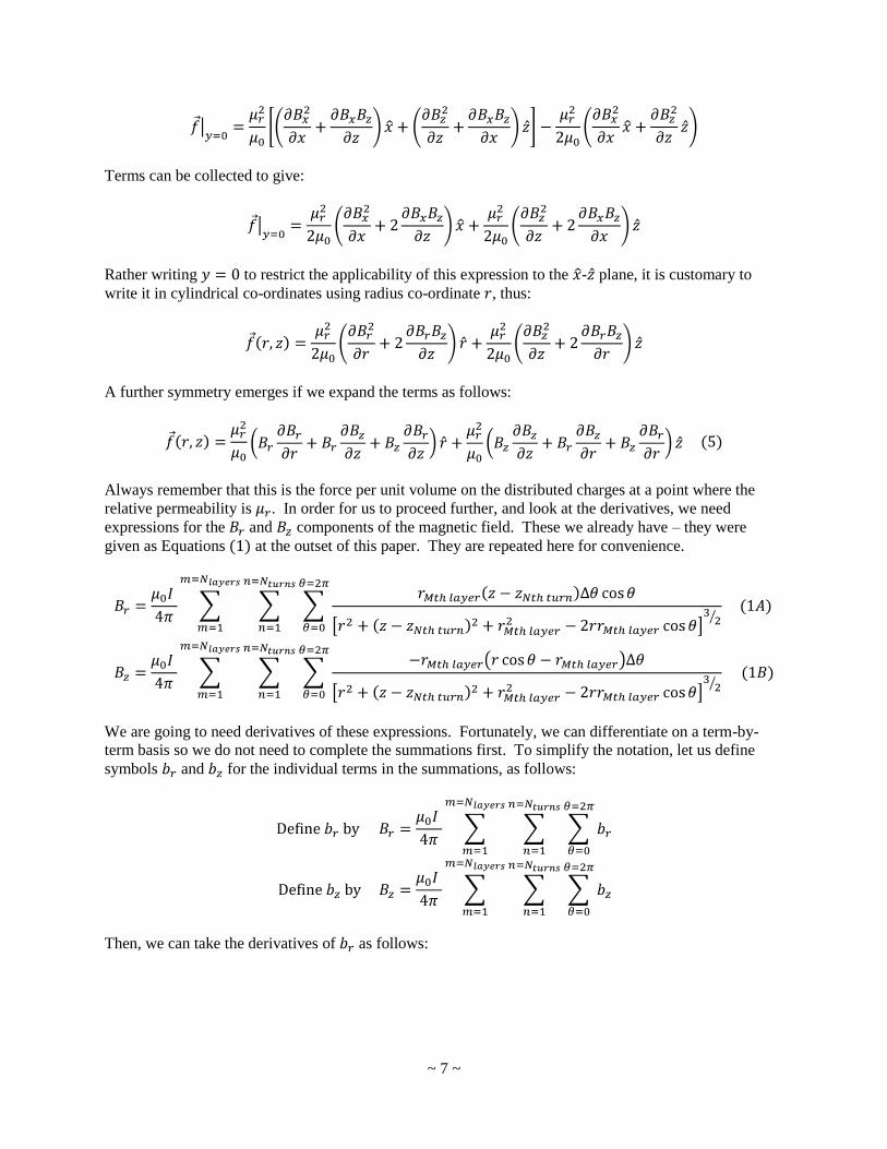
Terms can be collected to give:

Rather writing to restrict the applicability of this expression to the - plane, it is customary to

write it in cylindrical co-ordinates using radius co-ordinate , thus:

A further symmetry emerges if we expand the terms as follows:

Always remember that this is the force per unit volume on the distributed charges at a point where the

relative permeability is . In order for us to proceed further, and look at the derivatives, we need

expressions for the and components of the magnetic field. These we already have – they were

given as Equations at the outset of this paper. They are repeated here for convenience.

We are going to need derivatives of these expressions. Fortunately, we can differentiate on a term-by-

term basis so we do not need to complete the summations first. To simplify the notation, let us define

symbols and for the individual terms in the summations, as follows:

Then, we can take the derivatives of as follows:

~ 8 ~

and the derivatives of as follows:

A closed-form solution for these summations is just not possible. There are, however, regularities among

the six summations – the two components of the magnetic field and the four derivatives – which can

quicken the computations. All six summations have the form:

~ 9 ~

-Rcore

0

+Rcore

-6,000

-4,000

-2,000

0

2,000

4,000

6,000

-Hcoil -Hcoil/2 0+Hcoil/2 +Hcoil

Br(r,z)

where

and and for the six summations are:

We will see below that we really do not need all four derivatives, because certain symmetries are still at

play. Even so, let us evaluate them all for a sample configuration.

Sample calculation

Let us look at a sample solenoid. We will make it long (exactly equal to with a core

diameter of (exactly equal to three-quarters of an inch). This is long and thin. It is wound with

very heavy gauge wire – gauge enameled wire. This wire has an outside diameter of ,

which is a little more than one-sixteenth of an inch in diameter. Only turns can be wound along the

length of the solenoid. We will wind two layers to cancel out most of the helical effect.

The following two graphs show the radial component and axial component of the magnetic field

inside the core and for one-half coil’s length on either side. The plotted values do not include the constant

factor .

~ 10 ~

-Rcore

0

+Rcore

0

5,000

10,000

15,000

20,000

-Hcoil -Hcoil/2 0+Hcoil/2 +Hcoil

Bz(r,z)

In each graph, the horizontal axis is the axial displacement along the solenoid’s length. The location of

the ends of the solenoid, at the axial displacements of , are obvious. Note that the positive -

axis extends to the right, in the traditional manner, and that this is opposite to the direction of the -axis

shown in the first figure. The depth axis, which extends into the paper, is the radial displacement across

the diameter of the solenoid. The labels on the depth axis, showing that it extends from to

, are not strictly speaking accurate. The computations were only carried out to within 99% of the

solenoid’s radius.

The graph for shows that the axial component of the magnetic field is pretty uniform across and along

the interior of the solenoid. It falls off very quickly as one passes through either end. The radial

component is close to zero everywhere except very near to the “walls” and right at the ends.

There is a bit of ripple along the edges inside the solenoid. As one gets very near to the turns of wire, the

fields set up by the individual turns can be distinguished. Remember that the solenoid is wound using

very thick wire, whose centers are about one-sixteenth of an inch apart. Actually, the rippling seen is

more subtle than just the individual wires. It reflects some aliasing between the individual wires and the

step size of the numerical procedure. In order to create these graphs, the components of the magnetic

field were calculated at points in a rectangular grid. The grid was divided into points across the

diameter of the inside of the solenoid, from to . The axial dimension

was divided into points, from to . Therefore, the grid points were

separated by in the axial direction. The centers of the turns, on the other

hand, are apart. The grid spacing and the turn spacing are not exact multiples of one other. The

grid spacing is times greater than the turn spacing. The smallest (nearest)

integral multiple between the two spacing is about four times greater than this, since

The physical relationship between a given grid point and the nearby wires is repeated about

every fourth grid point. Four grid spacings is equal to ; turn spacings is

equal to . The pattern is repeated every fourth grid point. Since the solenoid

itself is grid points long, there will be repetitions of the pattern. It is for this reasons that there are

ripples along the edges of the curves above.

This phenomenon is not a mistake or computational error. It is a feature of the frequency of the display.

The and field strengths are correct at every grid point where they were calculated. If we had made

~ 11 ~

-Rcore

0

+Rcore

-2,000,000

-1,000,000

0

1,000,000

2,000,000

-Hcoil -Hcoil/2 0+Hcoil/2 +Hcoil

dBr(r,z)/dr

-Rcore

0

+Rcore

-1,500,000

-1,000,000

-500,000

0

500,000

1,000,000

1,500,000

-Hcoil -Hcoil/2 0+Hcoil/2 +Hcoil

dBr(r,z)/dz

the calculations at a different number of grid points, we would have seen a rippling pattern with a

different lineal frequency. If we divided the grid into a spacing which was small compared to the turn

spacing, then the pattern we would see would be the real pattern, which would recur with every turn, that

is, with a spacing of .

The following three graphs show the four derivatives in which we are interested. Once again, the plotted

values do not include the constant factor . The four derivatives are plotted at the same grid points

as the two field components.

~ 12 ~

-Rcore

0

-Rcore

-1,500,000

-1,000,000

-500,000

0

500,000

1,000,000

1,500,000

-Hcoil -Hcoil/2 0+Hcoil/2 +Hcoil

dBz(r,z)/dr

-Rcore

0

+Rcore

-3,000,000

-2,000,000

-1,000,000

0

1,000,000

2,000,000

3,000,000

-Hcoil -Hcoil/2 0+Hcoil/2 +Hcoil

dBz(r,z)/dz

It will take some close inspection and study to convince yourself that these four curves do, in fact,

represent the slopes of the surfaces in the first two graphs. The effect of the individual turns near the

walls is quite apparent. If we carried out the calculations on a fine enough grid, then there would be

ripples, corresponding to the number of turns of wire. They alternate in sign as one is alternately close to

one side or the other of the individual turns. This is a phenomenon which gets more pronounced as one

gets very close to the wires. Further away, deeper into the inside of the solenoid, the effects of the

individual wires becomes less pronounced. It also becomes less pronounced if the coil is wound with

thinner wire, in which case one must get even closer to the wires to distinguish their individual magnetic

fields.

One remarkable feature is the similarity, indeed identity, between the second and third graphs. It would

seem that . On second thought, this should not be too surprising after all. It is one

manifestation of the fourth one of Maxwell’s Equation, which itself is a version of Ampere’s Circuital

Law. In general:

~ 13 ~

Since there is no current density and no electric field inside the solenoid, the terms on the right-hand

side do not exist and the expression reduces to:

In our Cartesian co-ordinate frame, the curl on the left-hand side would be represented by the following

determinant:

If we, as usual, make the -axis a radial axis , so that the component of the magnetic field and the

derivatives in the -direction all vanish, then the expression reduces to:

If the two terms were not equal, then the curl would have a non-zero component in the -direction.

In due course below, we are going to be interested in the symmetry of the six graphed quantities around

the -axis. For the two components of the magnetic field:

For the four derivatives, we have:

Our use of the word asymmetric is not necessarily inconsistent with the magnetic field being the same in

every radial plane. For example, has the same magnitude for any given and , but is directed

outwards. It is the direction which gives rise to the so-called asymmetry in the table.

~ 14 ~

The Visual Basic routines which I used to carry out the calculations above and to save them in an Excel

file for plotting are listed in Appendix A attached hereto.

The six force components

Now, let us return to Equation , which gives the force per unit volume at any point . Six terms

contribute in equal measure to the force . Three contribute to the component of the force in the

radial direction and three contribute to the component of the force in the axial direction. I will refer to the

six terms as the six “force components”. They are:

Having already calculated the field components and derivatives at a set of grid points, it is an easy matter

to multiply the appropriate factors together. It is not necessary for us to review all of the results. In due

course below, we will add up contributions to the force in pairs, at points which are located on

opposite sides of the -axis. Any of the six force components which are radially asymmetric will vanish

when we pair the points in this way. The ones which will vanish are as follows:

All three terms which contribute to the radial component of will vanish. (We expect this, since it

is difficult to see how a configuration which is radially symmetric could give rise to a net force favouring

one radial direction over all others.) All three terms which contribute to the axial component of

will not vanish. We can therefore confine our attention to the last three of the six force components. The

following three graphs show these three force components. Since the individual field components and

derivatives were calculated without their constant factor , and since these three force components

are the products of a field component and a derivative, the values plotted do not include the constant

factor .

~ 15 ~

-Rcore

0

+Rcore

-2E+10

-1E+10

0

1E+10

2E+10

-Hcoil -Hcoil/2 0+Hcoil/2 +Hcoil

Bz(r,z) * dBz(r,z)/dz

-Rcore

0

+Rcore

-3E+09

-2E+09

-1E+09

0

1E+09

2E+09

3E+09

-Hcoil -Hcoil/2 0+Hcoil/2 +Hcoil

Br(r,z) * dBz(r,z)/dr

-Rcore

0

+Rcore

-1.5E+10

-1.0E+10

-5.0E+09

0.0E+00

5.0E+09

1.0E+10

1.5E+10

-Hcoil -Hcoil/2 0+Hcoil/2 +Hcoil

Bz(r,z) * dBr(r,z)/dr

~ 16 ~

-Rcore

0

-Rcore

-1E+10

-5E+09

0

5E+09

1E+10

-Hcoil-Hcoil/2 0

+Hcoil/2+Hcoil

Sum of three axial force components

-8E+09

-6E+09

-4E+09

-2E+09

0

2E+09

4E+09

6E+09

8E+09

-Hcoil -Hcoil/2 0 +Hcoil/2 +Hcoil

Components of force at r=5.81mm

#1

#3

Sum

The force depends on the sum of these three components. The following graph shows their sum.

Sorting out in one’s mind how the three components add up to this surface is not easy. It gets easier if we

look at a single cross-section of the surface. As an example, pick the radial distance . The

following graph shows two of the three force components, and their sum.

Aa glance at the individual graphs of the three force components shows that the second component, being

, is about an order of magnitude less than the other two. The curve immediately above shows

the first component in red and the third component in green. The first

component has almost exactly twice the magnitude of the second, and the two components have different

algebraic signs. It follows that their sum is very closely equal to one-half of the first component. Of

course, the components and their sum are non-zero only in the close vicinity of the ends of the coil. This

is the reason why the plunger on a working solenoid always extends through an end face.

~ 17 ~

The Visual Basic routines which I used to carry out the calculations above and to save them in an Excel

file for plotting are listed in Appendix B attached hereto.

The force on a thin disk

Up to this point, we have not done anything with the slug. We have looked at the magnetic field

generated by the solenoid. The calculations we have carried out, of the components of the magnetic field

and their derivatives, are useful whether or not there is a slug inside the coil. Or, more specifically,

whether or not there is any magnetic material at points inside the coil.

When a particular point is in air, or free space, then the magnetic field and its derivatives are

exactly as calculated above. When a particular point lies inside a bit of magnetic material, then the

magnetic field is increased by a factor equal to the relative permeability of the material. Since the

derivatives are linear operators on the components of the magnetic field, the derivatives will also be

multiplied by the factor .

When the point lies inside the slug, then Equation applies. Equation applies to any little bit

of volume which contains magnetic material. We developed Equation based in part on the radial

symmetry of the solenoid, but it applies at any point inside the slug, without regard to the shape of the

slug.

Although Equation holds for an irregularly-shaped slug, the mathematics are much easier if the slug is

also radially symmetric. This restricts the slug to being some combination of cylindrical and conical

shapes whose axes of symmetry are coincident with the -axis.

A good place to start is to imagine that the slug is a very thin disk, having radius and thickness

. We are going to assume that is very small, small enough to be considered a differential.

If we can calculate the force acting on such a disk, then we can easily add up the forces acting on a

succession of similar, neighbouring, disks which make up a real slug.

Now, the total force acting on the disk will be the sum of the forces acting on the small bits of

volume which make up the disk. In the limit, as the small bits of volume get very small, we can express

this as an integral:

There is a small conceptual leap in this equation. Force is the force which the external magnetic field

exerts on the free electrons in each element of volume, but force is the force on the disk as a rigid

body. There is a mechanism which makes them one and the same. Force pushes on the electrons and

they, in turn, push on the atoms in the matrix of the material. The atoms in the steel push back, in an

equal and opposite amount. The important point is that the force exerted by the external magnetic field is

transmitted to the matrix. If the matrix is free to move in response to the net applied force, that is, if the

steel slug is not held in place, it will be accelerated by the net force.

Note that, for convenience, I have temporarily reverted to the Cartesian frame of reference. We want to

divide the disk up into small elements of volume which will simplify the integration in Equation . The

following figure shows the thin disk, and a small segment of an annulus.

~ 18 ~

-axis

-axis

-axis

Convenient elements of volume for the integration are small segments of an annulus, having inner radius

and radial thickness . Let us use angle as the angle around the -axis, starting from the -axis, to

the center of the segment of annulus. Angle is then the angle subtended by the segment when viewed

from the -axis. We will take the thickness of the element of volume to be the thickness of the disk,

. The volume of the segment of annulus is:

As becomes very small, this expression reduces to:

In the limit, as the differences become small enough to be treated as differentials, it becomes:

and the integral can be written as:

If the disk is thin enough that the magnetic field and the force per unit volume are constant throughout the

disk’s thickness at any given radius and position angle , then we do not need to integrate over bits of

thickness , but can write:

~ 19 ~

Because of the radial symmetry of the thin disk, it is helpful to integrate over the angle first. For this

purpose, we will express the integral as:

Now, Equation above gives the force (at a point where the relative permeability is ) as:

When we integrate around the circle from to , all three of the terms in the radial direction

sum up to zero. We saw this above. Only the three terms in the axial direction survive. The integral

reduces to:

None of the three terms depends on angle . They are constant from the point-of-view of the integral

over . We can immediately write:

There are three terms which contribute to . Each one is the product of a magnetic field component

and a spatial derivative of a magnetic field component. Any particular term will not contribute much

unless both the component and the derivative are “high”, relatively speaking. For example, in regions

where the magnetic field is relatively constant, and its derivatives are small, there will be little

contribution to .

This has some important, and unfortunate, consequences (assuming that we want to be as big as

possible). A solenoid, and particularly a solenoid which is long compared to its radius, is noted for the

uniformity of the magnetic field inside. In fact, for an infinitely-long solenoid, the magnetic field does

not vary at all with axial displacement. The term with the derivative with respect to would contribute

nothing to the force. Furthermore, the magnetic field in a long solenoid is pretty much uniform across the

cross-section. Only near the walls will the derivatives with respect to be material.

Sample calculation continued

We do not need to specify physical parameters for the slug or, rather, a thin disk of it. The permeability

is a constant factor in the integral in Equation . The height, or length, of the slug does not matter

since we are considering a slice thick. To deal with the diameter of the disk, we can evaluate the

integral assuming the disk is some fraction or range of fractions of the solenoid’s core radius .

The following graph shows the force acting on a thin disk at various axial displacements along the length

of the solenoid. The forces are shown for disks having four different radii, the largest being

(exactly equal to one-half inch) in diameter. The other three are 40%, 60% and 80% of this diameter.

The vertical axis for values of the force do not include the factor of the integral in

~ 20 ~

-60,000

-30,000

0

30,000

60,000

-Hcoil -Hcoil/2 0 +Hcoil/2 +Hcoil

Force on thin disk

40%

60%

80%

100%

radius

-60,000

-50,000

-40,000

-30,000

-20,000

-10,000

0

-6.35cm +Hcoil/2 +6.35cm

Force on thin disk near face

40%

60%

80%

100%

radius

Equation . Furthermore, since the individual field components and derivatives were calculated

without their multiplicative factor , the values plotted for the force on a thin disk also do not

include the constant factor .

The force is zero everywhere except near the ends. To clarify things, the following graph shows that

portion of the near the face of the solenoid at axial displacement .

It appears as if the magnitude of the force on the thin disk is proportional to the radius of the disk. The

curves plotted are for radii of 40%, 60%, 80% and 100% of , and they are equally spaced. The

force is algebraically negative. It is directed towards the center of the solenoid and will attract the thin

disk into the interior of the solenoid. This curve shows the force at axial displacements within of

the end. The curve is not symmetry with respect to the face of the solenoid. The force is greatest just

inside the face. This is not as clear as it could be on the graph because the grid points at which the force

was calculated are apart.

~ 21 ~

-1000

-800

-600

-400

-200

0

200

400

600

800

1000

-Hcoil -Hcoil/2 0 +Hcoil/2 +Hcoil

Force on slug

The Visual Basic routines which I used to carry out the calculations for the thin disk and to save them in

an Excel file for plotting are listed in Appendix C attached hereto. The radius of the thin disk was divided

into radial annuli for the numerical integration. Where force components were needed for points

which were not grid points on the underlying grid, a linear interpolation was used.

Force on a slug

Now that we can calculate the force on a thin disk, we can easily place a number of such disks face-to-

face to build up a real slug. It is not necessary that the disk all have the same radius. The slug could be

composed of cylindrical and conical sections.

To get us started, let us consider a simple cylindrical slug, with radius being (so the

diameter is exactly equal to one-half inch) and length of (exactly equal to one inch). We

will assume that it is made from soft steel, with a relative permeability of . We will assume that

the applied magnetic field does not saturate the steel.

The following graph shows the force acting on the slug at various axial displacements along the length of

the solenoid. The vertical axis for values of the force does not include the factor of the integral

in Equation or the factor of the three force components.

The maximum value of the curve is approximately . This can be converted into a physical value, in

Newtons, by multiplying by the factors which were not included in the numerical work or on the graph:

~ 22 ~

-1000

-900

-800

-700

-600

-500

-400

-300

-200

-100

0

-6.35cm +Hcoil/2 +6.35cm

Florce on slug near face

Before completing this line of thought, it may be helpful to expand that part of the graph above to include

only the region near the face of the solenoid. The force on the slug, when its geometric center is within

of the face is shown in the following graph.

For the sake of comparison, I have shown as a sub-figure an outline of the slug and the solenoid on the

same scale as the horizontal axis ( ).

What limits the force on the slug?

Equation gives the maximum force on the slug, at the axial displacement where it is (almost) exactly

centered through a face of the solenoid. At other axials displacements, the force is less. In fact, it could

be said that the force on the slug is zero if it is more than three of its own lengths inside the solenoid or

two of its own lengths outside.

I have left Equation dependent on the current flowing through the solenoid and the permeability of

the material from which the slug is made. The force depends on the square of both parameters so

increasing them is important to maximizing the force on the slug. In theory, for example, one could use a

more and more powerful current supply to increase the current without bound. But, there is one thing to

prevent this. That other thing is the saturation point of the material. All materials have a saturation point,

which is the strength of the externally applied magnetic field beyond which the material shows no further

increase in its induced field. I have described the relative permeability by which the material

multiplies the strength of the external field. For soft steel, the relative permeability is often given as

. In other words, the total magnetic field at points within the steel is greater than the strength

of the externally-applied magnetic field. The electrons in the steel are very good at responding to an

external field.

But, as the externally-applied magnetic field gets stronger, there comes a point when all the electrons in

the steel have responded as much as they are able. Increasing the external field produces no further

effect. If the external field is generated by a solenoid, increasing the current beyond the point which

generates the saturation field strength is of no use – the magnetic field induced inside the steel cannot be

increased any more.

winding slug

~ 23 ~

Before we run an arbitrarily large current through the solenoid and calculate an arbitrarily large force on

the slug, we need to find out what the practical limit is. Let us place the slug half-way through one face

of the solenoid and calculate the maximum useful current.

In another paper, titled The magnetic field in and around a finite cylindrical air-core solenoid, I have

shown that the magnetic field strength at the center of a face of an empty solenoid is approximately equal

to:

and that the approximation becomes better as the solenoid becomes longer and thinner. The direction of

the field at the center of a face is exactly coincident with the -axis. The solenoid used in our sample

calculations is long and thin, so this expression is a very good approximateion. For that solenoid (without

a slug present), the magnetic field strength at a face-center is equal to:

If a soft steel slug is present in the end face, then the strength of the field is magnified by the relative

permeability, thus:

Now, I quote from Wikipedia, “For example, high permeability iron alloys used in transformers reach

magnetic saturation at , whereas ferrites saturate at . Some amorphous

alloys saturate at .” If our soft steel permeates at , then the maximum useful

current in the solenoid is given by:

Using a current greater than this would be a waste of power. The force on the slug at this level of current

is then given by Equation as:

Is a lot of force but not an astonishly large amount. The gravitational force on a one kilogram mass is

about on the surface of the Earth. A force is the same as the force of gravity acting on a

mass, which “weighs” about . That is the maximum amount of force our

solenoid can exert on our steel slug.

Jim Hawley

September 2011

An e-mail describing errors and omissions would be appreciated.

~ 24 ~

Appendix A

The following is a listing of the Visual Basic routines to calculate and save the two components of the

magnetic field and their four spatial derivatives. The routines were run using Microsoft’s Visual Basic

2010 Express.

Option Strict Off Option Explicit On Public Class Form1 Public Title As String = "Force on a slug" ' File handling. Public Filewriter As System.IO.StreamWriter Public Filereader As System.IO.StreamReader Public FieldTextFileName As String = "C:\FieldTextFile.txt" Public FieldPlotFileName As String = "C:\FieldPlotFile.xlsx" Public ForceComponentPlotFileName As String = "C:\ForceComponentPlotFile.xlsx" Public ForceOnThinDiskPlotFileName As String = "C:\ForceOnThinDiskPlotFile.xlsx" Public ForceOnSlugPlotFileName As String = "C:\ForceOnSlugPlotFile.xlsx" ' Six key summations are two field components and four derivatives. ' First dimension is 201 different values of the axial distance z. ' Second dimension is 201 different values of the radial distance r. Public Br(200, 200) As Double Public Bz(200, 200) As Double Public dBrdr(200, 200) As Double Public dBrdz(200, 200) As Double Public dBzdr(200, 200) As Double Public dBzdz(200, 200) As Double ' Three terms in the integral. ' First dimension is 201 different values of the axial distance z. ' Second dimension is 201 different values of the radial distance r. Public BzdBzdz(200, 200) As Double Public BzdBrdr(200, 200) As Double Public BrdBzdr(200, 200) As Double Public TotalBxdBxdx(200, 200) As Double ' Sum of the three components ' Force on a thin disk and slug. ' First dimension is 201 different values of the axial distance z. ' Second dimension contains varius disk radii. Public ForceOnDisk(200, 10) As Double Public ForceOnSlug(200) As Double ' Two spatial dimensions z (axial) and r (radial) Public Z As Double Public R As Double Public DelZ As Double Public DelR As Double ' Properties of the solenoid. Public Hcoil As Double = 0.635 ' 63.5 cm = 25 inches Public Rcore As Double = 0.01905 / 2 ' 1.905 cm = 3/4 inches Public Nturns As Int32 = 376 ' 63.5 cm / 376 = 1.69 mm, for #14 wire Public Nlayers As Int32 = 2 ' For calculations on a grid. Dim Zstart As Double = -Hcoil ' Examine Z one coil's length on either side Dim Zstop As Double = Hcoil Dim Rstart As Double = -0.99 * Rcore ' Examine R 99% of core radius on either side Dim Rstop As Double = 0.99 * Rcore Dim NumZ As Int32 = 201

~ 25 ~

Dim NumR As Int32 = 199 ' Properties of the slug. Public Rslug As Double = 0.0127 / 2 ' 1.27 cm = 1/2 inch Public Hslug As Double = 0.0254 ' 2.54 cm = 1 inch ' Summation variables. Public Theta As Double ' Angle around a solenoid turn Public CosTheta As Double ' Cosine of Theta Public DelTheta As Double ' Differental of Theta Public Zprime As Double ' Axial distance z Public DelZprime As Double ' Differential of axial distance z Public Numerator As Double Public Denominator As Double Public Denominator1 As Double Public Denominator2 As Double ' String handlers. Public TempString As String Public LenString As Int32 Sub New() InitializeComponent() With Me Size = New System.Drawing.Size(500, 300) Controls.Add(TextBox) TextBox.BringToFront() PerformLayout() Show() BringToFront() Refresh() End With Execute() End Sub Public TextBox As New Windows.Forms.TextBox() With _ {.Size = New System.Drawing.Size(450, 200), _ .Location = New System.Drawing.Point(25, 10), _ .Text = "", .TextAlign = HorizontalAlignment.Left, _ .Multiline = True} Sub Execute() Dim MsgBoxResult As MsgBoxResult MsgBoxResult = MsgBox("Calculate and save fields?", vbYesNo, Title) If (MsgBoxResult = vbYes) Then MsgBoxResult = MsgBox("Are you sure?", vbYesNo, "Re-calculate field") If (MsgBoxResult = vbYes) Then CalculateAndSaveFields(NumZ, NumR, Zstart, Zstop, Rstart, Rstop, _ Hcoil, Rcore, Nturns, Nlayers, FieldTextFileName) End If End If MsgBoxResult = MsgBox("Create Excel file for field?", vbYesNo, Title) If (MsgBoxResult = vbYes) Then ReadFieldFile(NumZ, NumR, Zstart, Zstop, Rstart, Rstop, _ Hcoil, Rcore, Nturns, Nlayers, FieldTextFileName) SaveFieldFileForPlotting(NumZ, NumR, Zstart, Zstop, Rstart, Rstop, _ Hcoil, Rcore, Nturns, Nlayers, FieldPlotFileName) End If MsgBox("All done") End Sub

~ 26 ~

'////////////////////////////////////////////////////////////////////////// '////////////////////////////////////////////////////////////////////////// ' CalculateAndSaveFields() is the principal numerical subroutine. It ' calculates the six summations -- the two components of the magnetic field ' and the four derivaties -- at NumZ * NumR different grid points. ' ' The grid is NumZ points wide and NumR points high. Where the grid starts ' and stops is determined by the arguments Zstart, Zstop, Rstart and Rstop. ' The grid points are spaced apart by (Zstop-Zstart)/(NumZ-1) and by ' (Rstart-Rstop)/(NumR-1). For all matrices, the Z-component is the first ' dimension and the R-component is the second dimension. ' ' The arguments Hcoil and Rcore and passed in as arguments. The number of ' turns and layers are passed in as the arguments Nturns and Nlayers. ' Note carefully that the wire's diameter is determined as WireD = ' Hcoil / Nturns. The user must make sure that all three quantities are ' consistent physically. ' ' Traverses around turns of the solenoid are done by dividing the circle ' into 2000 segments. ' ' The results do not include the factor: permeability of free space ' multiplied by the current and divided by 4pi. Calculation are carried ' out in the units supplied. They must be consistent, but need not be SI. ' ' Results are saved in a text file whose complete path name is passed in ' as an argument. ' Sub CalculateAndSaveFields( _ ByVal NumZ As Int32, ByVal NumR As Int32, _ ByVal Zstart As Double, ByVal Zstop As Double, _ ByVal Rstart As Double, ByVal Rstop As Double, _ ByVal Hcoil As Double, ByVal Rcore As Double, _ ByVal Nturns As Int32, ByVal Nlayers As Int32, _ ByVal FieldTextFileName As String) Dim WireD As Double Dim Rlayer As Double Dim Zturn As Double Dim Numerator0 As Double ' Temporary Rlayer * DelTheta Dim Numerator1 As Double ' Temporary Z - Zturn Dim Numerator2 As Double ' Temporary (Z - Zturn) * CosTheta Dim Numerator3 As Double ' Temporary (R * CosTheta) - Rlayer Dim Numerator4 As Double ' Temporary R - (Rlayer * CosTheta) Dim Denominator As Double ' Temporary variable Dim Denominator1 As Double ' Temporary variable Dim Denominator2 As Double ' Temporary variable Filewriter = New System.IO.StreamWriter(FieldTextFileName) ' Write header information to the text file. Filewriter.Write("Zstart= " & Trim(Str(Zstart)) & vbCrLf) Filewriter.Write("Zstop= " & Trim(Str(Zstop)) & vbCrLf) Filewriter.Write("Rstart= " & Trim(Str(Rstart)) & vbCrLf) Filewriter.Write("Rstop= " & Trim(Str(Rstop)) & vbCrLf) Filewriter.Write("NumZ= " & Trim(Str(NumZ)) & vbCrLf) Filewriter.Write("NumR= " & Trim(Str(NumR)) & vbCrLf) Filewriter.Write("Hcoil= " & Trim(Str(Hcoil)) & vbCrLf) Filewriter.Write("Rcore= " & Trim(Str(Rcore)) & vbCrLf) Filewriter.Write("Nturns= " & Trim(Str(Nturns)) & vbCrLf) Filewriter.Write("Nlayers= " & Trim(Str(Nlayers)) & vbCrLf)

~ 27 ~

' Set up constants. DelZ = (Zstop - Zstart) / (NumZ - 1) DelR = (Rstop - Rstart) / (NumR - 1) DelTheta = 2 * Math.PI / 2000 WireD = Hcoil / Nturns ' Loop over grid points in the axial z-direction. For Iz As Int32 = 0 To (NumZ - 1) Step 1 Z = Zstart + (Iz * DelZ) Filewriter.Write("Iz= " & Trim(Str(Iz)) & " Z= " & Trim(Str(Z)) & vbCrLf) ' Loop over grid points in the radial r-direction. For Ir As Int32 = 0 To (NumR - 1) Step 1 R = Rstart + (Ir * DelR) ' Initialize the six summations for this grid point. Br(Iz, Ir) = 0 Bz(Iz, Ir) = 0 dBrdr(Iz, Ir) = 0 dBrdz(Iz, Ir) = 0 dBzdr(Iz, Ir) = 0 dBzdz(Iz, Ir) = 0 ' Loop over layers in the solenoid. For Ilayer As Int32 = 1 To Nlayers Step 1 Rlayer = Rcore + ((Ilayer - 0.5) * WireD) Numerator0 = Rlayer * DelTheta ' Loop over the turns in the layer. For Iturn As Int32 = 1 To Nturns Step 1 Zturn = -(Hcoil / 2) + ((Iturn - 0.5) * WireD) Numerator1 = Z - Zturn ' Loop over segments around a turn. For Itheta As Int32 = 1 To 2000 Step 1 Theta = (Itheta - 0.5) * DelTheta CosTheta = Math.Cos(Theta) Numerator2 = Numerator1 * CosTheta Numerator3 = (R * CosTheta) - Rlayer Numerator4 = R - (Rlayer * CosTheta) Denominator = (R * R) + _ (Numerator1 * Numerator1) + _ (Rlayer * Rlayer) - _ (2 * R * Rlayer * CosTheta) Denominator1 = 1 / (Denominator * Math.Sqrt(Denominator)) Denominator2 = Denominator1 / Denominator ' Br Br(Iz, Ir) = Br(Iz, Ir) + _

(Numerator0 * Numerator2 * Denominator1) ' Bz Bz(Iz, Ir) = Bz(Iz, Ir) - _

(Numerator0 * Numerator3 * Denominator1) ' dBr/dr dBrdr(Iz, Ir) = dBrdr(Iz, Ir) - _ (3 * Numerator0 * Numerator2 * Numerator4 * Denominator2) ' dBr/dz dBrdz(Iz, Ir) = dBrdz(Iz, Ir) + _

(Numerator0 * CosTheta * Denominator1) dBrdz(Iz, Ir) = dBrdz(Iz, Ir) - _ (3 * Numerator0 * Numerator1 * Numerator2 * Denominator2) ' dBz/dr dBzdr(Iz, Ir) = dBzdr(Iz, Ir) - _

(Numerator0 * CosTheta * Denominator1) dBzdr(Iz, Ir) = dBzdr(Iz, Ir) + _

~ 28 ~

(3 * Numerator0 * Numerator3 * Numerator4 * Denominator2) ' dBz/dz dBzdz(Iz, Ir) = dBzdz(Iz, Ir) + _ (3 * Numerator0 * Numerator1 * Numerator3 * Denominator2) Next Itheta Next Iturn Next Ilayer ' Display progress to user TextBox.Text = "Iz=" & Str(Iz) & " Ir=" & Str(Ir) Me.Refresh() ' Write the six summations to the text file. Filewriter.Write("Ir= " & Trim(Str(Ir)) & " R= " & Trim(Str(R)) & vbCrLf) Filewriter.Write("Br= " & Trim(Str(Br(Iz, Ir))) & vbCrLf) Filewriter.Write("Bz= " & Trim(Str(Bz(Iz, Ir))) & vbCrLf) Filewriter.Write("dBrdr= " & Trim(Str(dBrdr(Iz, Ir))) & vbCrLf) Filewriter.Write("dBrdz= " & Trim(Str(dBrdz(Iz, Ir))) & vbCrLf) Filewriter.Write("dBzdr= " & Trim(Str(dBzdr(Iz, Ir))) & vbCrLf) Filewriter.Write("dBzdz= " & Trim(Str(dBzdz(Iz, Ir))) & vbCrLf) Next Ir Next Iz Filewriter.Close() End Sub '////////////////////////////////////////////////////////////////////////// '////////////////////////////////////////////////////////////////////////// ' ReadFieldFile() reads the data from the text file created by the ' subroutine CalculateAndSaveFields(). The text file name is passed in ' as the argument FieldFileName. All data is saved in the same variables ' from whence it originally came and is passed back to the calling routine ' as ByRef arguments. Sub ReadFieldFile( _ ByRef NumZ As Int32, ByRef NumR As Int32, _ ByRef Zstart As Double, ByRef Zstop As Double, _ ByRef Rstart As Double, ByRef Rstop As Double, _ ByRef Hcoil As Double, ByRef Rcore As Double, _ ByRef Nturns As Int32, ByRef Nlayers As Int32, _ ByVal FieldTextFileName As String) Filereader = New System.IO.StreamReader(FieldTextFileName) Try TempString = Filereader.ReadLine() If (Strings.Left(TempString, 7) <> "Zstart=") Then MsgBox("Error in line Zstart=") Application.Exit() Else Zstart = Val(Strings.Right(TempString, Len(TempString) - 7)) End If TempString = Filereader.ReadLine() If (Strings.Left(TempString, 6) <> "Zstop=") Then MsgBox("Error in line Zstop=") Application.Exit() Else Zstop = Val(Strings.Right(TempString, Len(TempString) - 6)) End If TempString = Filereader.ReadLine() If (Strings.Left(TempString, 7) <> "Rstart=") Then MsgBox("Error in line Rstart=") Application.Exit() Else

~ 29 ~

Rstart = Val(Strings.Right(TempString, Len(TempString) - 7)) End If TempString = Filereader.ReadLine() If (Strings.Left(TempString, 6) <> "Rstop=") Then MsgBox("Error in line Rstop=") Application.Exit() Else Rstop = Val(Strings.Right(TempString, Len(TempString) - 6)) End If TempString = Filereader.ReadLine() If (Strings.Left(TempString, 5) <> "NumZ=") Then MsgBox("Error in line NumZ=") Application.Exit() Else NumZ = CInt(Val(Strings.Right(TempString, Len(TempString) - 5))) End If TempString = Filereader.ReadLine() If (Strings.Left(TempString, 5) <> "NumR=") Then MsgBox("Error in line NumR=") Application.Exit() Else NumR = CInt(Val(Strings.Right(TempString, Len(TempString) - 5))) End If TempString = Filereader.ReadLine() If (Strings.Left(TempString, 6) <> "Hcoil=") Then MsgBox("Error in line Hcoil=") Application.Exit() Else Hcoil = Val(Strings.Right(TempString, Len(TempString) - 6)) End If TempString = Filereader.ReadLine() If (Strings.Left(TempString, 6) <> "Rcore=") Then MsgBox("Error in line Rcore=") Application.Exit() Else Rcore = Val(Strings.Right(TempString, Len(TempString) - 6)) End If TempString = Filereader.ReadLine() If (Strings.Left(TempString, 7) <> "Nturns=") Then MsgBox("Error in line Nturns=") Application.Exit() Else Nturns = CInt(Val(Strings.Right(TempString, Len(TempString) - 7))) End If TempString = Filereader.ReadLine() If (Strings.Left(TempString, 8) <> "Nlayers=") Then MsgBox("Error in line Nlayers=") Application.Exit() Else Nlayers = CInt(Val(Strings.Right(TempString, Len(TempString) - 8))) End If For Iz = 0 To (NumZ - 1) Step 1 ' Display progress to user TextBox.Text = "Reading Iz=" & Str(Iz) Me.Refresh() TempString = Filereader.ReadLine() If (Strings.Left(TempString, 3) <> "Iz=") Then MsgBox("Expected Iz= and read " & TempString)

~ 30 ~

Application.Exit() End If TempString = Strings.Right(TempString, Len(TempString) - 3) If (Val(TempString) <> Iz) Then MsgBox("Error in line Iz= " & TempString) Application.Exit() End If For Ir = 0 To (NumR - 1) Step 1 TempString = Filereader.ReadLine() If (Strings.Left(TempString, 3) <> "Ir=") Then MsgBox("Expected Ir= and read " & TempString) Application.Exit() End If TempString = Strings.Right(TempString, Len(TempString) - 3) If (Val(TempString) <> Ir) Then MsgBox("Error in line Ir= " & TempString) Application.Exit() End If ' Read Br TempString = Filereader.ReadLine() If (Strings.Left(TempString, 3) <> "Br=") Then MsgBox("Error in Br= when Iz= " & Str(Iz) & _

" and Ir= " & Str(Ir)) Application.Exit() End If TempString = Strings.Right(TempString, Len(TempString) - 3) Br(Iz, Ir) = Val(TempString) ' Read Bz TempString = Filereader.ReadLine() If (Strings.Left(TempString, 3) <> "Bz=") Then MsgBox("Error in Bz= when Iz= " & Str(Iz) & _

" and Ir= " & Str(Ir)) Application.Exit() End If TempString = Strings.Right(TempString, Len(TempString) - 3) Bz(Iz, Ir) = Val(TempString) ' Read dBr/dr TempString = Filereader.ReadLine() If (Strings.Left(TempString, 6) <> "dBrdr=") Then MsgBox("Error in dBrdr= when Iz= " & Str(Iz) & _

" and Ir= " & Str(Ir)) Application.Exit() End If TempString = Strings.Right(TempString, Len(TempString) - 6) dBrdr(Iz, Ir) = Val(TempString) ' Read dBr/dz TempString = Filereader.ReadLine() If (Strings.Left(TempString, 6) <> "dBrdz=") Then MsgBox("Error in dBrdz= when Iz= " & Str(Iz) & _

" and Ir= " & Str(Ir)) Application.Exit() End If TempString = Strings.Right(TempString, Len(TempString) - 6) dBrdz(Iz, Ir) = Val(TempString) ' Read dBz/dr TempString = Filereader.ReadLine() If (Strings.Left(TempString, 6) <> "dBzdr=") Then MsgBox("Error in dBzdr= when Iz= " & Str(Iz) & _

~ 31 ~

" and Ir= " & Str(Ir)) Application.Exit() End If TempString = Strings.Right(TempString, Len(TempString) - 6) dBzdr(Iz, Ir) = Val(TempString) ' Read dBz/dz TempString = Filereader.ReadLine() If (Strings.Left(TempString, 6) <> "dBzdz=") Then MsgBox("Error in dBzdz= when Iz= " & Str(Iz) & _

" and Ir= " & Str(Ir)) Application.Exit() End If TempString = Strings.Right(TempString, Len(TempString) - 6) dBzdz(Iz, Ir) = Val(TempString) Next Ir Next Iz Filereader.Close() Catch e As Exception MsgBox("Error reading field file") Application.Exit() End Try End Sub '////////////////////////////////////////////////////////////////////////// '////////////////////////////////////////////////////////////////////////// ' SaveFieldFileForPlotting() saves the six summations -- the two magnetic ' field components and the four derivatives -- in an Excel file for ' plotting purposes. The complete path name of the Excel file is passed ' in as an argument. Do not forget that all variables must exist before ' calling this subroutine. Sub SaveFieldFileForPlotting( _ ByVal NumZ As Int32, ByVal NumR As Int32, _ ByVal Zstart As Double, ByVal Zstop As Double, _ ByVal Rstart As Double, ByVal Rstop As Double, _ ByVal Hcoil As Double, ByVal Rcore As Double, _ ByVal Nturns As Int32, ByVal Nlayers As Int32, _ ByVal FieldPlotFileName As String) Dim objExcel As Microsoft.Office.Interop.Excel.Application Dim objExcelWB As Microsoft.Office.Interop.Excel.Workbook Dim objExcelWS As Microsoft.Office.Interop.Excel.Worksheet Dim WireD As Double Dim DelZ As Double Dim DelR As Double Dim RowNum As Int32 Dim TempNum As Double ' Open Excel file. Try objExcel = CType(CreateObject("Excel.Application"), _ Microsoft.Office.Interop.Excel.Application) objExcel.Visible = False objExcelWB = CType(objExcel.Workbooks.Open(FieldPlotFileName), _ Microsoft.Office.Interop.Excel.Workbook) objExcelWS = CType(objExcelWB.Sheets("Sheet1"), _

Microsoft.Office.Interop.Excel.Worksheet) Catch ex As Exception Cursor.Current = Cursors.Default MsgBox("Could not open the Excel file.", vbOKOnly) Application.Exit()

~ 32 ~

End Try ' Write header information into Excel file. objExcelWS.Cells(1, 1) = "Magnetic field data from VB program" objExcelWS.Cells(2, 1) = "Zstart=" objExcelWS.Cells(2, 2) = Trim(Str(Zstart)) objExcelWS.Cells(3, 1) = "Zstop=" objExcelWS.Cells(3, 2) = Trim(Str(Zstop)) objExcelWS.Cells(4, 1) = "NumZ=" objExcelWS.Cells(4, 2) = Trim(Str(NumZ)) objExcelWS.Cells(5, 1) = "Rstart=" objExcelWS.Cells(5, 2) = Trim(Str(Rstart)) objExcelWS.Cells(6, 1) = "Rstop=" objExcelWS.Cells(6, 2) = Trim(Str(Rstop)) objExcelWS.Cells(7, 1) = "NumR=" objExcelWS.Cells(7, 2) = Trim(Str(NumR)) objExcelWS.Cells(8, 1) = "Hcoil=" objExcelWS.Cells(8, 2) = Trim(Str(Hcoil)) objExcelWS.Cells(9, 1) = "Rcore=" objExcelWS.Cells(9, 2) = Trim(Str(Rcore)) objExcelWS.Cells(10, 1) = "Nturns=" objExcelWS.Cells(10, 2) = Trim(Str(Nturns)) objExcelWS.Cells(11, 1) = "Nlayers=" objExcelWS.Cells(11, 2) = Trim(Str(Nlayers)) WireD = Hcoil / Nturns objExcelWS.Cells(12, 1) = "WireD=" objExcelWS.Cells(12, 2) = Trim(Str(WireD)) DelZ = (Zstop - Zstart) / (NumZ - 1) objExcelWS.Cells(13, 1) = "DelZ=" objExcelWS.Cells(13, 2) = Trim(Str(DelZ)) DelR = (Rstop - Rstart) / (NumR - 1) objExcelWS.Cells(13, 1) = "DelR=" objExcelWS.Cells(13, 2) = Trim(Str(DelR)) ' Write z-co-ordinates across the page. RowNum = 15 objExcelWS.Cells(RowNum, 1) = "Iz=" objExcelWS.Cells(RowNum + 1, 1) = "Z=" For Iz As Int32 = 0 To (NumZ - 1) Step 1 objExcelWS.Cells(RowNum, 5 + Iz) = Trim(Str(Iz)) TempNum = Zstart + (Iz * DelZ) objExcelWS.Cells(RowNum + 1, 5 + Iz) = Trim(Str(TempNum)) Next Iz ' Write block of Br data. RowNum = RowNum + 3 objExcelWS.Cells(RowNum, 1) = "***** Field component Br *****" For Ir As Int32 = 0 To (NumR - 1) Step 1 TextBox.Text = "Writing Br data for Ir=" & Str(Ir) ' Display progress to user Me.Refresh() RowNum = RowNum + 1 objExcelWS.Cells(RowNum, 1) = "Ir=" objExcelWS.Cells(RowNum, 2) = Trim(Str(Ir)) TempNum = Rstart + (Ir * DelR) objExcelWS.Cells(RowNum, 3) = "R=" objExcelWS.Cells(RowNum, 4) = Trim(Str(TempNum)) For Iz As Int32 = 0 To (NumZ - 1) Step 1 objExcelWS.Cells(RowNum, 5 + Iz) = Trim(Str(Br(Iz, Ir))) Next Iz Next Ir ' Write block of Bz data.

~ 33 ~

RowNum = RowNum + 2 objExcelWS.Cells(RowNum, 1) = "***** Field component Bz *****" For Ir As Int32 = 0 To (NumR - 1) Step 1 TextBox.Text = "Writing Bz data for Ir=" & Str(Ir) ' Display progress to user Me.Refresh() RowNum = RowNum + 1 objExcelWS.Cells(RowNum, 1) = "Ir=" objExcelWS.Cells(RowNum, 2) = Trim(Str(Ir)) TempNum = Rstart + (Ir * DelR) objExcelWS.Cells(RowNum, 3) = "R=" objExcelWS.Cells(RowNum, 4) = Trim(Str(TempNum)) For Iz As Int32 = 0 To (NumZ - 1) Step 1 objExcelWS.Cells(RowNum, 5 + Iz) = Trim(Str(Bz(Iz, Ir))) Next Iz Next Ir ' Write block of dBr/dr data. RowNum = RowNum + 2 objExcelWS.Cells(RowNum, 1) = "***** Derivative dBr/dr *****" For Ir As Int32 = 0 To (NumR - 1) Step 1 TextBox.Text = "Writing dBr/dr data for Ir=" & Str(Ir) ' Display progress Me.Refresh() RowNum = RowNum + 1 objExcelWS.Cells(RowNum, 1) = "Ir=" objExcelWS.Cells(RowNum, 2) = Trim(Str(Ir)) TempNum = Rstart + (Ir * DelR) objExcelWS.Cells(RowNum, 3) = "R=" objExcelWS.Cells(RowNum, 4) = Trim(Str(TempNum)) For Iz As Int32 = 0 To (NumZ - 1) Step 1 objExcelWS.Cells(RowNum, 5 + Iz) = Trim(Str(dBrdr(Iz, Ir))) Next Iz Next Ir ' Write block of dBr/dz data. RowNum = RowNum + 2 objExcelWS.Cells(RowNum, 1) = "***** Derivative dBr/dz *****" For Ir As Int32 = 0 To (NumR - 1) Step 1 TextBox.Text = "Writing dBr/dz data for Ir=" & Str(Ir) ' Display progress Me.Refresh() RowNum = RowNum + 1 objExcelWS.Cells(RowNum, 1) = "Ir=" objExcelWS.Cells(RowNum, 2) = Trim(Str(Ir)) TempNum = Rstart + (Ir * DelR) objExcelWS.Cells(RowNum, 3) = "R=" objExcelWS.Cells(RowNum, 4) = Trim(Str(TempNum)) For Iz As Int32 = 0 To (NumZ - 1) Step 1 objExcelWS.Cells(RowNum, 5 + Iz) = Trim(Str(dBrdz(Iz, Ir))) Next Iz Next Ir ' Write block of dBz/dr data. RowNum = RowNum + 2 objExcelWS.Cells(RowNum, 1) = "***** Derivative dBz/dr *****" For Ir As Int32 = 0 To (NumR - 1) Step 1 TextBox.Text = "Writing dBz/dr data for Ir=" & Str(Ir) ' Display progress Me.Refresh() RowNum = RowNum + 1 objExcelWS.Cells(RowNum, 1) = "Ir=" objExcelWS.Cells(RowNum, 2) = Trim(Str(Ir)) TempNum = Rstart + (Ir * DelR) objExcelWS.Cells(RowNum, 3) = "R="

~ 34 ~

objExcelWS.Cells(RowNum, 4) = Trim(Str(TempNum)) For Iz As Int32 = 0 To (NumZ - 1) Step 1 objExcelWS.Cells(RowNum, 5 + Iz) = Trim(Str(dBzdr(Iz, Ir))) Next Iz Next Ir ' Write block of dBz/dz data. RowNum = RowNum + 2 objExcelWS.Cells(RowNum, 1) = "***** Derivative dBz/dz *****" For Ir As Int32 = 0 To (NumR - 1) Step 1 TextBox.Text = "Writing dBz/dz data for Ir=" & Str(Ir) ' Display progress Me.Refresh() RowNum = RowNum + 1 objExcelWS.Cells(RowNum, 1) = "Ir=" objExcelWS.Cells(RowNum, 2) = Trim(Str(Ir)) TempNum = Rstart + (Ir * DelR) objExcelWS.Cells(RowNum, 3) = "R=" objExcelWS.Cells(RowNum, 4) = Trim(Str(TempNum)) For Iz As Int32 = 0 To (NumZ - 1) Step 1 objExcelWS.Cells(RowNum, 5 + Iz) = Trim(Str(dBzdz(Iz, Ir))) Next Iz Next Ir objExcelWB.Save() objExcelWB.Close() End Sub End Class

~ 35 ~

Appendix B

The following is a listing of the Visual Basic routines to calculate and save the three force components.

The routines were run using Microsoft’s Visual Basic 2010 Express.

Add the following to subroutine Execute():

MsgBoxResult = MsgBox("Create Excel file for force components?", vbYesNo, Title) If (MsgBoxResult = vbYes) Then ReadFieldFile(NumZ, NumR, Zstart, Zstop, Rstart, Rstop, _ Hcoil, Rcore, Nturns, Nlayers, FieldTextFileName) CalculateForceComponents(NumZ, NumR) SaveForceComponentFileForPlotting(NumZ, NumR, Zstart, Zstop, Rstart, Rstop, _ Hcoil, Rcore, Nturns, Nlayers, ForceComponentPlotFileName) End If

Add the following subroutines: '////////////////////////////////////////////////////////////////////////// '////////////////////////////////////////////////////////////////////////// ' CalculateForceComponents() calculates the three axial terms of the ' force at each grid point where the two magnetic field components and ' the four derivatives are known. Do not forget that all variables must ' exist before calling this subroutine. Sub CalculateForceComponents( _ ByVal NumZ As Int32, ByVal NumR As Int32) For Iz As Int32 = 0 To (NumZ - 1) Step 1

For Ir As Int32 = 0 To (NumR - 1) Step 1 BzdBzdz(Iz, Ir) = Bz(Iz, Ir) * dBzdz(Iz, Ir) BrdBzdr(Iz, Ir) = Br(Iz, Ir) * dBzdr(Iz, Ir) BzdBrdr(Iz, Ir) = Bz(Iz, Ir) * dBrdr(Iz, Ir) TotalBxdBxdx(Iz, Ir) = BzdBzdz(Iz, Ir) + BrdBzdr(Iz, Ir) + BzdBrdr(Iz, Ir) Next Ir Next Iz

End Sub

'////////////////////////////////////////////////////////////////////////// '////////////////////////////////////////////////////////////////////////// ' SaveForceComponentFileForPlotting() saves the three axial terms of the ' force in an Excel file for plotting purposes. The complete path name of ' the Excel file is passed in as an argument. Do not forget that all ' variables must exist before calling this subroutine. Sub SaveForceComponentFileForPlotting( _ ByVal NumZ As Int32, ByVal NumR As Int32, _ ByVal Zstart As Double, ByVal Zstop As Double, _ ByVal Rstart As Double, ByVal Rstop As Double, _ ByVal Hcoil As Double, ByVal Rcore As Double, _ ByVal Nturns As Int32, ByVal Nlayers As Int32, _ ByVal ForceComponentPlotFileName As String) Dim objExcel As Microsoft.Office.Interop.Excel.Application Dim objExcelWB As Microsoft.Office.Interop.Excel.Workbook Dim objExcelWS As Microsoft.Office.Interop.Excel.Worksheet Dim WireD As Double Dim DelZ As Double Dim DelR As Double Dim RowNum As Int32 Dim TempNum As Double

~ 36 ~

' Open Excel file. Try objExcel = CType(CreateObject("Excel.Application"), _ Microsoft.Office.Interop.Excel.Application) objExcel.Visible = False objExcelWB = CType(objExcel.Workbooks.Open(ForceComponentPlotFileName), _ Microsoft.Office.Interop.Excel.Workbook) objExcelWS = CType(objExcelWB.Sheets("Sheet1"), _ Microsoft.Office.Interop.Excel.Worksheet) Catch ex As Exception Cursor.Current = Cursors.Default MsgBox("Could not open the Excel file.", vbOKOnly) Application.Exit() End Try ' Write header information into Excel file. objExcelWS.Cells(1, 1) = "Force axial component data from VB program" objExcelWS.Cells(2, 1) = "Zstart=" objExcelWS.Cells(2, 2) = Trim(Str(Zstart)) objExcelWS.Cells(3, 1) = "Zstop=" objExcelWS.Cells(3, 2) = Trim(Str(Zstop)) objExcelWS.Cells(4, 1) = "NumZ="

objExcelWS.Cells(4, 2) = Trim(Str(NumZ)) objExcelWS.Cells(5, 1) = "Rstart=" objExcelWS.Cells(5, 2) = Trim(Str(Rstart)) objExcelWS.Cells(6, 1) = "Rstop=" objExcelWS.Cells(6, 2) = Trim(Str(Rstop)) objExcelWS.Cells(7, 1) = "NumR=" objExcelWS.Cells(7, 2) = Trim(Str(NumR)) objExcelWS.Cells(8, 1) = "Hcoil=" objExcelWS.Cells(8, 2) = Trim(Str(Hcoil)) objExcelWS.Cells(9, 1) = "Rcore=" objExcelWS.Cells(9, 2) = Trim(Str(Rcore)) objExcelWS.Cells(10, 1) = "Nturns=" objExcelWS.Cells(10, 2) = Trim(Str(Nturns)) objExcelWS.Cells(11, 1) = "Nlayers=" objExcelWS.Cells(11, 2) = Trim(Str(Nlayers)) WireD = Hcoil / Nturns objExcelWS.Cells(12, 1) = "WireD=" objExcelWS.Cells(12, 2) = Trim(Str(WireD)) DelZ = (Zstop - Zstart) / (NumZ - 1) objExcelWS.Cells(13, 1) = "DelZ=" objExcelWS.Cells(13, 2) = Trim(Str(DelZ)) DelR = (Rstop - Rstart) / (NumR - 1) objExcelWS.Cells(13, 1) = "DelR=" objExcelWS.Cells(13, 2) = Trim(Str(DelR)) ' Write z-co-ordinates across the page. RowNum = 15 objExcelWS.Cells(RowNum, 1) = "Iz=" objExcelWS.Cells(RowNum + 1, 1) = "Z=" For Iz As Int32 = 0 To (NumZ - 1) Step 1 objExcelWS.Cells(RowNum, 5 + Iz) = Trim(Str(Iz)) TempNum = Zstart + (Iz * DelZ) objExcelWS.Cells(RowNum + 1, 5 + Iz) = Trim(Str(TempNum)) Next Iz ' Write block of Bz * dBz/dz data. RowNum = RowNum + 3 objExcelWS.Cells(RowNum, 1) = "***** Force component Bz * dBz/dz *****" For Ir As Int32 = 0 To (NumR - 1) Step 1

~ 37 ~

RowNum = RowNum + 1 objExcelWS.Cells(RowNum, 1) = "Ir=" objExcelWS.Cells(RowNum, 2) = Trim(Str(Ir)) TempNum = Rstart + (Ir * DelR) objExcelWS.Cells(RowNum, 3) = "R=" objExcelWS.Cells(RowNum, 4) = Trim(Str(TempNum)) For Iz As Int32 = 0 To (NumZ - 1) Step 1 objExcelWS.Cells(RowNum, 5 + Iz) = Trim(Str(BzdBzdz(Iz, Ir))) TextBox.Text = "Writing Bz * dBz/dz data for Ir=" & Str(Ir) & _ " and Iz=" & Str(Iz) ' Display progress to user Me.Refresh() Next Iz Next Ir ' Write block of Br * dBz/dr data. RowNum = RowNum + 2 objExcelWS.Cells(RowNum, 1) = "***** Force component Br * dBz/dr *****" For Ir As Int32 = 0 To (NumR - 1) Step 1 RowNum = RowNum + 1 objExcelWS.Cells(RowNum, 1) = "Ir=" objExcelWS.Cells(RowNum, 2) = Trim(Str(Ir)) TempNum = Rstart + (Ir * DelR) objExcelWS.Cells(RowNum, 3) = "R=" objExcelWS.Cells(RowNum, 4) = Trim(Str(TempNum)) For Iz As Int32 = 0 To (NumZ - 1) Step 1 objExcelWS.Cells(RowNum, 5 + Iz) = Trim(Str(BrdBzdr(Iz, Ir))) TextBox.Text = "Writing Br * dBz/dr data for Ir=" & Str(Ir) & _ " and Iz=" & Str(Iz) ' Display progress to user Me.Refresh() Next Iz Next Ir ' Write block of Bz * dBr/dr data. RowNum = RowNum + 2 objExcelWS.Cells(RowNum, 1) = "***** Force component Bz * dBr/dr *****" For Ir As Int32 = 0 To (NumR - 1) Step 1 RowNum = RowNum + 1 objExcelWS.Cells(RowNum, 1) = "Ir=" objExcelWS.Cells(RowNum, 2) = Trim(Str(Ir)) TempNum = Rstart + (Ir * DelR) objExcelWS.Cells(RowNum, 3) = "R=" objExcelWS.Cells(RowNum, 4) = Trim(Str(TempNum)) For Iz As Int32 = 0 To (NumZ - 1) Step 1 objExcelWS.Cells(RowNum, 5 + Iz) = Trim(Str(BzdBrdr(Iz, Ir))) TextBox.Text = "Writing Bz * dBr/dr data for Ir=" & Str(Ir) & _ " and Iz=" & Str(Iz) ' Display progress to user Me.Refresh() Next Iz Next Ir ' Write block of Total Bx * dBx/dx data. RowNum = RowNum + 2 objExcelWS.Cells(RowNum, 1) = "***** Total force Bx * dBx/dx *****" For Ir As Int32 = 0 To (NumR - 1) Step 1 RowNum = RowNum + 1 objExcelWS.Cells(RowNum, 1) = "Ir=" objExcelWS.Cells(RowNum, 2) = Trim(Str(Ir)) TempNum = Rstart + (Ir * DelR) objExcelWS.Cells(RowNum, 3) = "R=" objExcelWS.Cells(RowNum, 4) = Trim(Str(TempNum)) For Iz As Int32 = 0 To (NumZ - 1) Step 1

~ 38 ~

objExcelWS.Cells(RowNum, 5 + Iz) = Trim(Str(TotalBxdBxdx(Iz, Ir))) TextBox.Text = "Writing Total Bx * dBx/dx data for Ir=" & Str(Ir) & _ " and Iz=" & Str(Iz) ' Display progress to user Me.Refresh() Next Iz Next Ir objExcelWB.Save() objExcelWB.Close()

End Sub

~ 39 ~

Appendix C

The following is a listing of the Visual Basic routines to calculate and save the force on a thin disk at

various axial displacements. The routines were run using Microsoft’s Visual Basic 2010 Express.

Add the following to subroutine Execute():

MsgBoxResult = MsgBox("Create Excel file for force on thin disk?", vbYesNo, Title) If (MsgBoxResult = vbYes) Then ReadFieldFile(NumZ, NumR, Zstart, Zstop, Rstart, Rstop, _ Hcoil, Rcore, Nturns, Nlayers, FieldTextFileName) CalculateForceComponents(NumZ, NumR) For I As Int32 = 1 To 4 Step 1 Select Case I Case 1 CalculateForceOnThinDisk(NumZ, NumR, Rstart, Rstop, 0.4 * Rslug, 1) Case 2 CalculateForceOnThinDisk(NumZ, NumR, Rstart, Rstop, 0.6 * Rslug, 2) Case 3 CalculateForceOnThinDisk(NumZ, NumR, Rstart, Rstop, 0.8 * Rslug, 3) Case 4 CalculateForceOnThinDisk(NumZ, NumR, Rstart, Rstop, Rslug, 4) Case Else MsgBox("Unrecognized disk radius") Application.Exit() End Select Next I SaveForceOnThinDiskFileForPlotting(NumZ, NumR, Zstart, Zstop, Rstart, Rstop, _ Hcoil, Rcore, Nturns, Nlayers, 4, ForceOnThinDiskPlotFileName) End If

Add the following subroutines: '////////////////////////////////////////////////////////////////////////// '////////////////////////////////////////////////////////////////////////// ' CalculateForceOnThinDisk() calculates the force acting on a thin disk. ' The results are saved in ForceOnDisk(*,RadiusIndex), where RadiusIndex ' can be up to 10. The first dimension is the axial displacement at the ' grid points. Enough radius information needs to be passed to this ' subroutine so that it can integrate across the face of the disk. ' The integral is carried out in 1000 steps and values of the force ' components are interpolated linearly from those at the known grid points. ' Do not forget that all variables must exist before calling this ' subroutine. Sub CalculateForceOnThinDisk( _ ByVal NumZ As Int32, ByVal NumR As Int32, _ ByVal Rstart As Double, ByVal Rstop As Double, _ ByVal Rslug As Double, ByVal RadiusIndex As Int32) Dim DelRgrid As Double = (Rstop - Rstart) / (NumR - 1) Dim DelRdisk As Double = Rslug / 1000 Dim IgridLow As Int32 ' Lower bound for interpolation Dim IgridHigh As Int32 ' Lower bound for interpolation Dim RdiskMid As Double ' Mid-point of radial segment on disk Dim IntBzdBzdz As Double ' Interpolated value Dim IntBzdBrdr As Double ' Interpolated value Dim IntBrdBzdr As Double ' Interpolated value For Iz As Int32 = 0 To (NumZ - 1) Step 1

~ 40 ~

' Initialize the cumulative total. ForceOnDisk(Iz, RadiusIndex) = 0 For Ir As Int32 = 1 To 1000 Step 1 RdiskMid = (Ir - 0.5) * DelRdisk ' Provisionally calculate the nearest surrounding grid points. IgridLow = CInt(RdiskMid / DelRgrid) IgridHigh = IgridLow + 1 ' Ensure that RgridLow is less than or equal to RdiskMid. If (IgridLow * DelRgrid > RdiskMid) Then IgridLow = IgridLow - 1 IgridHigh = IgridLow + 1 End If ' Ensure that RgridHigh is greater than or equal to RdiskMid. If (IgridHigh * DelRgrid < RdiskMid) Then IgridLow = IgridLow - 1 IgridHigh = IgridLow + 1 End If ' Interpolate the force components from the surrounding grid points. IntBzdBzdz = BzdBzdz(Iz, IgridLow) + _ ((RdiskMid - (IgridLow * DelRgrid)) * _ (BzdBzdz(Iz, IgridHigh) - BzdBzdz(Iz, IgridLow)) / DelRgrid) IntBzdBrdr = BzdBrdr(Iz, IgridLow) + _ ((RdiskMid - (IgridLow * DelRgrid)) * _ (BzdBrdr(Iz, IgridHigh) - BzdBrdr(Iz, IgridLow)) / DelRgrid) IntBrdBzdr = BrdBzdr(Iz, IgridLow) + _ ((RdiskMid - (IgridLow * DelRgrid)) * _ (BrdBzdr(Iz, IgridHigh) - BrdBzdr(Iz, IgridLow)) / DelRgrid) ' Add the increment to the integral. ForceOnDisk(Iz, RadiusIndex) = ForceOnDisk(Iz, RadiusIndex) + _ (RdiskMid * IntBzdBzdz * DelRdisk) + _ (RdiskMid * IntBzdBrdr * DelRdisk) + _ (RdiskMid * IntBrdBzdr * DelRdisk) Next Ir Next Iz End Sub '////////////////////////////////////////////////////////////////////////// '////////////////////////////////////////////////////////////////////////// ' SaveForceOnThinDiskFileForPlotting() saves the force on a thin disk in ' an Excel file for plotting purposes. The complete path name of the ' Excel file is passed in as an argument. Do not forget that all ' variables must exist before calling this subroutine. Sub SaveForceOnThinDiskFileForPlotting( _ ByVal NumZ As Int32, ByVal NumR As Int32, _ ByVal Zstart As Double, ByVal Zstop As Double, _ ByVal Rstart As Double, ByVal Rstop As Double, _ ByVal Hcoil As Double, ByVal Rcore As Double, _ ByVal Nturns As Int32, ByVal Nlayers As Int32, _ ByVal MaxRadiusIndex As Int32, _ ByVal ForceOnThinDiskPlotFileName As String) Dim objExcel As Microsoft.Office.Interop.Excel.Application Dim objExcelWB As Microsoft.Office.Interop.Excel.Workbook Dim objExcelWS As Microsoft.Office.Interop.Excel.Worksheet Dim WireD As Double Dim DelZ As Double Dim DelR As Double Dim RowNum As Int32 Dim TempNum As Double

~ 41 ~

' Open Excel file. Try objExcel = CType(CreateObject("Excel.Application"), _ Microsoft.Office.Interop.Excel.Application) objExcel.Visible = False objExcelWB = CType(objExcel.Workbooks.Open(ForceOnThinDiskPlotFileName), _ Microsoft.Office.Interop.Excel.Workbook)

objExcelWS = CType(objExcelWB.Sheets("Sheet1"), _ Microsoft.Office.Interop.Excel.Worksheet)

Catch ex As Exception Cursor.Current = Cursors.Default MsgBox("Could not open the Excel file.", vbOKOnly) Application.Exit() End Try ' Write header information into Excel file. objExcelWS.Cells(1, 1) = "Force on thin disk from VB program" objExcelWS.Cells(2, 1) = "Zstart=" objExcelWS.Cells(2, 2) = Trim(Str(Zstart)) objExcelWS.Cells(3, 1) = "Zstop=" objExcelWS.Cells(3, 2) = Trim(Str(Zstop)) objExcelWS.Cells(4, 1) = "NumZ=" objExcelWS.Cells(4, 2) = Trim(Str(NumZ)) objExcelWS.Cells(5, 1) = "Rstart=" objExcelWS.Cells(5, 2) = Trim(Str(Rstart)) objExcelWS.Cells(6, 1) = "Rstop=" objExcelWS.Cells(6, 2) = Trim(Str(Rstop)) objExcelWS.Cells(7, 1) = "NumR=" objExcelWS.Cells(7, 2) = Trim(Str(NumR)) objExcelWS.Cells(8, 1) = "Hcoil=" objExcelWS.Cells(8, 2) = Trim(Str(Hcoil)) objExcelWS.Cells(9, 1) = "Rcore=" objExcelWS.Cells(9, 2) = Trim(Str(Rcore)) objExcelWS.Cells(10, 1) = "Nturns=" objExcelWS.Cells(10, 2) = Trim(Str(Nturns)) objExcelWS.Cells(11, 1) = "Nlayers=" objExcelWS.Cells(11, 2) = Trim(Str(Nlayers)) WireD = Hcoil / Nturns objExcelWS.Cells(12, 1) = "WireD=" objExcelWS.Cells(12, 2) = Trim(Str(WireD)) DelZ = (Zstop - Zstart) / (NumZ - 1) objExcelWS.Cells(13, 1) = "DelZ=" objExcelWS.Cells(13, 2) = Trim(Str(DelZ)) DelR = (Rstop - Rstart) / (NumR - 1) objExcelWS.Cells(13, 1) = "DelR=" objExcelWS.Cells(13, 2) = Trim(Str(DelR)) ' Write headers across the page. objExcelWS.Cells(17, 1) = "Iz" objExcelWS.Cells(17, 2) = "Z" For RadiusIndex As Int32 = 1 To MaxRadiusIndex Step 1 objExcelWS.Cells(15, 2 + RadiusIndex) = "Radius" objExcelWS.Cells(16, 2 + RadiusIndex) = "Index" objExcelWS.Cells(17, 2 + RadiusIndex) = "# " & Trim(Str(RadiusIndex)) Next RadiusIndex ' Write the ForceOnDisk data. RowNum = 18 For Iz As Int32 = 0 To (NumZ - 1) Step 1 RowNum = RowNum + 1 objExcelWS.Cells(RowNum, 1) = Trim(Str(Iz))

~ 42 ~

TempNum = Zstart + (Iz * DelZ) objExcelWS.Cells(RowNum, 2) = Trim(Str(TempNum)) For RadiusIndex As Int32 = 1 To MaxRadiusIndex Step 1 objExcelWS.Cells(RowNum, 2 + RadiusIndex) = _ Trim(Str(ForceOnDisk(Iz, RadiusIndex))) Next RadiusIndex Next Iz objExcelWB.Save() objExcelWB.Close() End Sub

~ 43 ~

Appendix D

The following is a listing of the Visual Basic routines to calculate and save the force on a cylindrical slug

in the solenoid at various axial displacements. The routines were run using Microsoft’s Visual Basic

2010 Express.

Add the following to subroutine Execute():

MsgBoxResult = MsgBox("Calculate force on slug?", vbYesNo, "Force on slug") If (MsgBoxResult = vbYes) Then ReadFieldFile(NumZ, NumR, Zstart, Zstop, Rstart, Rstop, _ Hcoil, Rcore, Nturns, Nlayers, FieldTextFileName) TextBox.Text = "Now calculating force components" Me.Refresh() CalculateForceComponents(NumZ, NumR) TextBox.Text = "Now calculating forces on a thin disk" Me.Refresh() CalculateForceOnThinDisk(NumZ, NumR, Rstart, Rstop, Rslug, 1) TextBox.Text = "Now calculating forces on a slug" Me.Refresh() CalculateForceOnSlug(NumZ, NumR, Zstart, Zstop, Rslug, Hslug) TextBox.Text = "Now saving forces on a slug" SaveForceOnSlugFileForPlotting(NumZ, NumR, Zstart, Zstop, Rstart, Rstop, _ Hcoil, Rcore, Nturns, Nlayers, Rslug, Hslug, ForceOnslugPlotFileName) End If

Add the following subroutines: '////////////////////////////////////////////////////////////////////////// '////////////////////////////////////////////////////////////////////////// ' CalculateForceOnSlug() calculates the force acting on a slug. The ' results are saved in ForceOnSlug(), where the dimension is the axial ' displacement of the geometric center of the slug. The subroutine does ' not calculate the force if any part of the slug lies outside of the grid ' at which the magnetic data has been calaculated. In those case, the ' entry in ForceOnSlug() is left at zero. The slug is divided axially ' into 500 thin disks. Before calling this subroutine, the subroutine ' CalculateForceOnThinDisk() must be called and vector ForceonDisk(,1) ' loaded at all axial displacements on the grid with the force on a disk ' with the same radius as the slug. The values of the force on the thin ' at axial displacements which are not on the grid are interpolated ' linearly from those at the known grid points. Do not forget that all ' variables must exist before calling this subroutine. Sub CalculateForceOnSlug( _ ByVal NumZ As Int32, ByVal NumR As Int32, _ ByVal Zstart As Double, ByVal Zstop As Double, _ ByVal Rslug As Double, ByVal Hslug As Double) Dim DelZgrid As Double = (Zstop - Zstart) / (NumZ - 1) Dim IgridLow As Int32 ' Lower bound for interpolation Dim IgridHigh As Int32 ' Lower bound for interpolation Dim ZslugMid As Double ' Axial mid-point of the slug Dim ZslugMax As Double ' Axial displacement of positive face of the slug Dim ZslugMin As Double ' Axial displacement of negative face of the slug Dim ZdiskMid As Double ' Axial mid-point of a thin disk in the slug Dim IntForceOnDisk As Double ' Interpolated value of force on a thin disk For Iz As Int32 = 0 To (NumZ - 1) Step 1 ZslugMid = Iz * DelZgrid

~ 44 ~

ZslugMax = ZslugMid + (0.5 * Hslug) ZslugMin = ZslugMid - (0.5 * Hslug) Do ' Do not calculate if the negative end of the slug is outside the grid. If (ZslugMin < 0) Then ForceOnSlug(Iz) = 0 Exit Do End If ' Do not calculate if the positive end of the slug is outside the grid. If (ZslugMax > ((NumZ - 1) * DelZgrid)) Then ForceOnSlug(Iz) = 0 Exit Do End If ' Initialize the cumulative total. ForceOnSlug(Iz) = 0 For Idisk As Int32 = 1 To 500 Step 1 ZdiskMid = ZslugMin + (Idisk - 0.5) * Hslug / 500 ' Provisionally calculate the nearest surrounding grid points. IgridLow = CInt(ZdiskMid / DelZgrid) IgridHigh = IgridLow + 1 ' Ensure that ZgridLow is less than or equal to ZdiskMid. If (IgridLow * DelZgrid > ZdiskMid) Then IgridLow = IgridLow - 1 IgridHigh = IgridLow + 1 End If ' Ensure that ZgridHigh is greater than or equal to ZdiskMid. If (IgridHigh * DelZgrid < ZdiskMid) Then IgridLow = IgridLow - 1 IgridHigh = IgridLow + 1 End If ' Interpolate the force components from the surrounding grid points. IntForceOnDisk = ForceOnDisk(IgridLow, 1) + _ ((ZdiskMid - (IgridLow * DelZgrid)) * _ (ForceOnDisk(IgridHigh, 1) - ForceOnDisk(IgridLow, 1)) / DelZgrid) ' Add the increment to the integral. ForceOnSlug(Iz) = ForceOnSlug(Iz) + (IntForceOnDisk * Hslug / 500) Next Idisk Exit Do Loop ' Display progress to user. TextBox.Text = "Calculating force at Iz = " & Trim(Str(Iz)) Me.Refresh() Next Iz End Sub '////////////////////////////////////////////////////////////////////////// '////////////////////////////////////////////////////////////////////////// ' SaveForceOnSlugForPlotting() saves the force on a slug in an Excel file ' for plotting purposes. The complete path name of the Excel file is ' passed in as an argument. Do not forget that all variables must exist ' before calling this subroutine. Sub SaveForceOnSlugFileForPlotting( _ ByVal NumZ As Int32, ByVal NumR As Int32, _ ByVal Zstart As Double, ByVal Zstop As Double, _ ByVal Rstart As Double, ByVal Rstop As Double, _ ByVal Hcoil As Double, ByVal Rcore As Double, _ ByVal Nturns As Int32, ByVal Nlayers As Int32, _ ByVal Rslug As Double, ByVal Hslug As Double, _

~ 45 ~

ByVal ForceOnSlugPlotFileName As String) Dim objExcel As Microsoft.Office.Interop.Excel.Application Dim objExcelWB As Microsoft.Office.Interop.Excel.Workbook Dim objExcelWS As Microsoft.Office.Interop.Excel.Worksheet Dim WireD As Double Dim DelZ As Double Dim DelR As Double Dim RowNum As Int32 Dim TempNum As Double ' Open Excel file. Try objExcel = CType(CreateObject("Excel.Application"), _ Microsoft.Office.Interop.Excel.Application) objExcel.Visible = False objExcelWB = CType(objExcel.Workbooks.Open(ForceOnSlugPlotFileName), _ Microsoft.Office.Interop.Excel.Workbook) objExcelWS = CType(objExcelWB.Sheets("Sheet1"), _ Microsoft.Office.Interop.Excel.Worksheet) Catch ex As Exception Cursor.Current = Cursors.Default MsgBox("Could not open the Excel file.", vbOKOnly) Application.Exit() End Try ' Write header information into Excel file. objExcelWS.Cells(1, 1) = "Force on slug from Force_On_Steel_Slug VB program" objExcelWS.Cells(2, 1) = "Zstart=" objExcelWS.Cells(2, 2) = Trim(Str(Zstart)) objExcelWS.Cells(3, 1) = "Zstop=" objExcelWS.Cells(3, 2) = Trim(Str(Zstop)) objExcelWS.Cells(4, 1) = "NumZ=" objExcelWS.Cells(4, 2) = Trim(Str(NumZ)) objExcelWS.Cells(5, 1) = "Rstart=" objExcelWS.Cells(5, 2) = Trim(Str(Rstart)) objExcelWS.Cells(6, 1) = "Rstop=" objExcelWS.Cells(6, 2) = Trim(Str(Rstop)) objExcelWS.Cells(7, 1) = "NumR=" objExcelWS.Cells(7, 2) = Trim(Str(NumR)) objExcelWS.Cells(8, 1) = "Hcoil=" objExcelWS.Cells(8, 2) = Trim(Str(Hcoil)) objExcelWS.Cells(9, 1) = "Rcore=" objExcelWS.Cells(9, 2) = Trim(Str(Rcore)) objExcelWS.Cells(10, 1) = "Nturns=" objExcelWS.Cells(10, 2) = Trim(Str(Nturns)) objExcelWS.Cells(11, 1) = "Nlayers=" objExcelWS.Cells(11, 2) = Trim(Str(Nlayers)) WireD = Hcoil / Nturns objExcelWS.Cells(12, 1) = "WireD=" objExcelWS.Cells(12, 2) = Trim(Str(WireD)) DelZ = (Zstop - Zstart) / (NumZ - 1) objExcelWS.Cells(13, 1) = "DelZ=" objExcelWS.Cells(13, 2) = Trim(Str(DelZ)) DelR = (Rstop - Rstart) / (NumR - 1) objExcelWS.Cells(13, 1) = "DelR=" objExcelWS.Cells(13, 2) = Trim(Str(DelR)) objExcelWS.Cells(14, 1) = "Rslug=" objExcelWS.Cells(14, 2) = Trim(Str(Rslug)) objExcelWS.Cells(15, 1) = "Hslug=" objExcelWS.Cells(15, 2) = Trim(Str(Hslug))

~ 46 ~

' Write headers across the page. objExcelWS.Cells(17, 1) = "Iz" objExcelWS.Cells(17, 2) = "Z" objExcelWS.Cells(17, 3) = "Force" ' Write the ForceOnSlug data. RowNum = 18 For Iz As Int32 = 0 To (NumZ - 1) Step 1 RowNum = RowNum + 1 objExcelWS.Cells(RowNum, 1) = Trim(Str(Iz)) TempNum = Zstart + (Iz * DelZ) objExcelWS.Cells(RowNum, 2) = Trim(Str(TempNum)) objExcelWS.Cells(RowNum, 3) = Trim(Str(ForceOnSlug(Iz))) Next Iz objExcelWB.Save() objExcelWB.Close() End Sub