******* basic effect size computations using ... es computations, p. 1 basic effect size guide with...
TRANSCRIPT
Basic ES Computations, p. 1
BASIC EFFECT SIZE GUIDE WITH SPSS AND SAS SYNTAX Gregory J. Meyer, Robert E. McGrath, and Robert Rosenthal
Last updated January 13, 2003
Pending:
1. Formulas for repeated measures/paired samples. (d = r / sqrt(1-r^2)
2. Explanation of 'set aside' lambda weights of 0 when computing focused contrasts.
3. Applications to multifactor designs.
SECTION I: COMPUTING EFFECT SIZES FROM RAW DATA.
I-A. The Pearson Correlation as the Effect Size
I-A-1: Calculating Pearson's r From a Design With a Dimensional Variable and a Dichotomous
Variable (i.e., a t-Test Design).
I-A-2: Calculating Pearson's r From a Design With Two Dichotomous Variables (i.e., a 2 x 2
Chi-Square Design).
I-A-3: Calculating Pearson's r From a Design With a Dimensional Variable and an Ordered,
Multi-Category Variable (i.e., a Oneway ANOVA Design).
I-A-4: Calculating Pearson's r From a Design With One Variable That Has 3 or More Ordered
Categories and One Variable That Has 2 or More Ordered Categories (i.e., an Omnibus
Chi-Square Design with df > 1).
I-B. Cohen's d as the Effect Size
I-B-1: Calculating Cohen's d From a Design With a Dimensional Variable and a Dichotomous
Variable (i.e., a t-Test Design).
SECTION II: COMPUTING EFFECT SIZES FROM THE OUTPUT OF STATISTICAL
TESTS AND TRANSLATING ONE EFFECT SIZE TO ANOTHER.
II-A. The Pearson Correlation as the Effect Size
II-A-1: Pearson's r From t-Test Output Comparing Means Across Two Groups.
II-A-2: Pearson's r From 2 x 2 Chi-Square Output.
II-A-3. Pearson's r From F Test Output When Just Two Groups Have Been Compared.
II-A-4: Pearson's r From F Test Output When More Than Two Groups Have Been Compared.
II-A-4-a: Scenario 1 - When given group Ms and F or t from a focused contrast
II-A-4-b: Scenario 2 - When given group Ms, SDs, and ns
II-A-4-c: Scenario 3 - When given group Ms and results from an omnibus F test
II-A-5: Pearson's r From the Output of an Omnibus Chi-Square Test (i.e., df > 1).
II-A-5-a: The Rosnow and Rosenthal (1996) approach
II-A-5-b: Reconstructing the database
II-A-6. Pearson's r from Cohen's d.
II-A-6-a: The exact formula.
II-A-6-b: The approximate formula.
II-B. Cohen's d as the Effect Size
II-B-1: Cohen's d from t-Test Output.
II-B-1-a: When the size of each group is known.
II-B-1-b: When the size of each group is unknown but df is available.

Basic ES Computations, p. 2
II-B-2: Cohen's d From F Test Output When Just Two Groups Have Been Compared.
II-B-3: Cohen's d from Pearson's r.
General Note: When computing r and d according to the procedures in this guide, r and d are
effect size measures like those used in a meta-analysis. As such, r and d should be given a
positive sign when the result is consistent with the a priori hypothesis and a negative sign when
the result is in the direction opposite of that specified by the hypothesis. This point is emphasized
throughout the guide and should be stated in the text of any manuscript reporting these results.
Basic ES Computations, p. 3
******************************************************************************
SECTION I: COMPUTING EFFECT SIZES FROM RAW DATA.
******************************************************************************
I-A. The Pearson Correlation as the Effect Size
I-A-1: Calculating Pearson's r From a Design With a Dimensional Variable and a Dichotomous
Variable (i.e., a t-Test Design).
In a t-test design there is one dichotomous variable and one variable that is dimensional. To
compute r in this situation we code (or recode) the dichotomous variable so it takes on the values
-1 and 1 (although any two values could be used). After this is done we simply correlate the
dichotomous variable with the dimensional variable. This type of correlation is often referred to
as a point-biserial correlation but it is simply Pearson's r with one variable continuous and one
variable dichotomous. In other words, a point-biserial correlation is not different from a Pearson
correlation.
To compute r from this kind of design using SPSS or SAS syntax, we open the dataset
containing raw scores on our dichotomous and dimensional variables. For the sake of simplicity,
the following commands assume that these two variables have been labeled "dichot_v" and
"dimen_v", respectively. The syntax below will have to be modified so that the correct variable
names from your dataset replace "dichot_v" and "dimen_v". Note that the variable "dichot_v"
has to be coded so that it has two numerical values (e.g., -1 and 1).
In SPSS syntax the command would be as follows. CORRELATIONS /VARIABLES= dimen_v dichot_v
/PRINT=TWOTAIL SIG
/MISSING=PAIRWISE .
In SAS syntax the commands would be as follows. PROC CORR;
VAR dimen_v dichot_v;
RUN;
Note. When variances are not equal (e.g., by Levene's test for the equality of variances), the p
value associated with this correlation may be incorrect. A more accurate estimate of p can be
obtained by running a t-test (using "dichot_v" as the grouping variable) in SPSS or SAS and
obtaining p from the t-test output that corrects for unequal variances. Although it is appropriate
to use the unequal variance t-test output to obtain p, it is not appropriate to use this output to
convert t to r via the formula given elsewhere in this document.
Note. The sign of this correlation is arbitrary. When the direction of the result is consistent with
the a priori hypothesis, it should be reported with a positive sign. When the result is in the
direction opposite of that specified by the hypothesis, it should be given a negative sign. This is
easily accomplished by giving the group expected to have the higher mean the larger value on
dichot_v.

Basic ES Computations, p. 4
I-A-2: Calculating Pearson's r From a Design With Two Dichotomous Variables (i.e., a 2 x 2
Chi-Square Design).
In a 2x2 chi-square design there are two dichotomous variables. To compute r, each of the
dichotomous variables should be coded so scores take on the values -1 and 1 (although any two
values could be used). Next, we correlate the first dichotomous variable with the second
dichotomous variable. This type of correlation is often referred to as a phi coefficient but it is
simply Pearson's r with both variables dichotomous. In other words, a phi coefficient is not
different from a Pearson correlation.
To compute r from this kind of design using SPSS or SAS syntax, we open the dataset
containing raw scores on our two dichotomous variables. For the sake of simplicity, the
following syntax commands assume that these two variables have been labeled "dichot_a" and
"dichot_b" and the syntax will have to be modified so it uses the correct variable names for your
dataset.
The SPSS syntax is as follows. CORRELATIONS /VARIABLES= dichot_a dichot_b
/PRINT=TWOTAIL SIG
/MISSING=PAIRWISE .
The SAS syntax is as follows. PROC CORR;
VAR dichot_a dichot_b;
RUN;
Note. The sign of the correlations produced by any of the above commands is arbitrary. When
the direction of the result is consistent with the a priori hypothesis, it should be reported with a
positive sign. When the result turns out to be in the direction opposite of that specified by the
hypothesis, it should be given a negative sign. This is easily accomplished by assigning the
larger values on dichot_a and dichot_b in such a way that the hypothesized association leads to a
positive correlation. For instance, if patients with T-Scores > 65 on MMPI-2 Scale 2 are
expected to receive a depressive diagnosis more often than patients with T-Scores < 66, the
MMPI variable could be coded as T > 65 = 1 and T < 66 = -1, while the diagnosis variable would
then be coded as not-depressed = -1 and depressed = 1.
Note. When N is very small (e.g., below 20) and any expected cell frequencies are less than 5, a
more accurate way to obtain r is through a several step process based on Fisher's Exact Test.
Specifically, we a) compute Fisher's Exact Test, b) obtain the one-tailed p value associated with
this test, c) convert the p value to a t value, and then d) compute r from that t and the
corresponding degrees of freedom (df = N – 2). These steps are explained and illustrated below.
a) Fisher's Exact Test is produced by the chi-square facility in SPSS or SAS (which can also be
used to compute phi directly). Using the initial data set described above (i.e., with the raw data
for our two variables, "dichot_a" and "dichot_b") we run the following syntax commands.
In SPSS, the syntax is as follows. CROSSTABS
/TABLES= dichot_a BY dichot_b
Basic ES Computations, p. 5
/FORMAT= AVALUE TABLES
/STATISTIC= CHISQ PHI CORR
/CELLS= COUNT .
In SAS, the syntax would be as follows. PROC FREQ;
TABLES dichot_a*dichot_b / CHISQ;
RUN;
b) To obtain the one-tailed p from the Fisher's Exact Test output, it may be necessary to change
the default output settings in SPSS or SAS so that p is reported to at least 2 non-zero digits. In
other words, r cannot be obtained if the output reports "p < .000". Instead, we must obtain the
actual p value to at least two meaningful digits (e.g., p = .000054 or p = .000000013).
c) Once the correct p value is obtained, we convert this value to t. (Note that in this instance, it is
more accurate to convert p to t than it is to convert p to Z, the standard normal deviate.) To do so
in SPSS or SAS, we use the inverse distribution function for t. Several steps are required. First in
a new dataset create a variable labeled "p_by_FET" (to indicate it is for the p obtained from
Fisher's Exact Test) and a second variable labeled "df" (to indicate degrees of freedom). Next,
enter the observed p value from the Fisher's Exact Test in the p_by_FET column and enter N - 2
in the df column. Finally, run the following syntax.
In SPSS: COMPUTE t_by_p = IDF.T((1 - p_by_fet),df) .
EXECUTE .
In SAS: DATA newdata;
SET olddata;
t_by_p = TINV((1 - p_by_fet,df);
RUN;
d) Next, we compute r from the t value just obtained. For this step, we use the same data set and
just run one additional command. The command takes the t value from Step "c" and transforms it
to r. The following syntax commands are used.
In SPSS: COMPUTE r_by_t = sqrt((t_by_p**2) / ((t_by_p**2) + df)).
EXECUTE .
In SAS: DATA newdata;
SET olddata;
r_by_t = sqrt((t_by_p**2) / ((t_by_p**2) + df));
RUN;
Basic ES Computations, p. 6
I-A-3: Calculating Pearson's r From a Design With a Dimensional Variable and an Ordered,
Multi-Category Variable (i.e., an ANOVA Design).
An ANOVA design contains one variable with multiple discrete categories and one variable that
is dimensional. In a true or quasi-experiment, the multi-category variable is the independent
variable (IV) and the dimensional variable is the dependent variable (DV). However, when
computing an effect size, the multi-category variable does not need to be a manipulated
independent variable. The multi-category variable may be a predictor variable but this also is not
a requirement. It may be the criterion variable when the predictor variable is dimensional. In
other words, when computing an effect size, the traditional IV and DV classifications are not
important.
When the multi-category variable can be ordered on a hypothesized continuum, the hypothesized
order forms what is called a focused contrast. The focused contrast specifies how the means on
the dimensional variable should be arrayed across the discrete categories (i.e., it says which
categories should have high, low, and midrange values). To compute r from an ANOVA design
with a hypothesized focused contrast, two steps may be required.
First, if the multi-category variable has not already been coded on an ordered continuum that
corresponds to the hypothesis, this must be done. For instance, assume the multi-category
variable is treatment outcome that is classified into three groups: unchanged, improved, and
worse. In addition, assume that the dimensional variable is a test scale of psychological resilience
that was obtained before treatment began. The hypothesis for this study is that higher levels of
psychological resilience at baseline will predict better outcome.
Given this hypothesis, the multi-category variable should be coded so that worse outcome = -1,
unchanged outcome = 0, and improved outcome = 1. [See Table 4 in Rosnow, Rosenthal, and
Rubin's (2000) Psychological Science article for contrast weights that are appropriate to use
when the multi-category variable has 2 to 10 categories.] When the multi-category variable in a
data set is recoded so that the categories correspond to the hypothesized ordered continuum, the
variable should be given a new name to reflect this change. In this example, the recoded outcome
variable is given the name "cntrst_v" to indicate that it is now a variable coded in accordance
with the hypothesized focused contrast; i.e., a higher score indicates greater improvement.
Once the multi-category variable is coded so that each category has been assigned a contrast
weight consistent with the hypothesis, the second and final step is to correlate the recoded multi-
category variable (cntrst_v) with the dimensional variable (labeled dimen_v in the syntax
below). In the running example, test scores of resilience (i.e., dimen_v) would be correlated with
the multi-category variable (i.e., cntrst_v) that has been coded to indicate treatment outcome
consistent with our hypothesis (worse = -1, unchanged = 0, improved = 1).
In SPSS syntax: CORRELATIONS /VARIABLES= cntrst_v dimen_v
/PRINT=TWOTAIL SIG
/MISSING=PAIRWISE .
In SAS syntax: SAS:
Basic ES Computations, p. 7
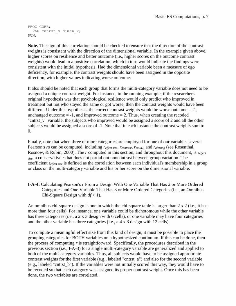
PROC CORR;
VAR cntrst_v dimen_v;
RUN;
Note. The sign of this correlation should be checked to ensure that the direction of the contrast
weights is consistent with the direction of the dimensional variable. In the example given above,
higher scores on resilience and better outcome (i.e., higher scores on the outcome contrast
weights) would lead to a positive correlation, which in turn would indicate the findings were
consistent with the initial hypothesis. Had the dimensional variable been a measure of ego
deficiency, for example, the contrast weights should have been assigned in the opposite
direction, with higher values indicating worse outcome.
It also should be noted that each group that forms the multi-category variable does not need to be
assigned a unique contrast weight. For instance, in the running example, if the researcher's
original hypothesis was that psychological resilience would only predict who improved in
treatment but not who stayed the same or got worse, then the contrast weights would have been
different. Under this hypothesis, the correct contrast weights would be worse outcome = -1,
unchanged outcome = -1, and improved outcome = 2. Thus, when creating the recoded
"cntrst_v" variable, the subjects who improved would be assigned a score of 2 and all the other
subjects would be assigned a score of -1. Note that in each instance the contrast weights sum to
0.
Finally, note that when three or more categories are employed for one of our variables several
Pearson's rs can be computed, including reffect size, rcontrast, rBESD, and ralerting (see Rosenthal,
Rosnow, & Rubin, 2000). The r computed in this section, and throughout this document, is reffect
size, a conservative r that does not partial out noncontrast between group variation. The
coefficient reffect size is defined as the correlation between each individual's membership in a group
or class on the multi-category variable and his or her score on the dimensional variable.
I-A-4: Calculating Pearson's r From a Design With One Variable That Has 2 or More Ordered
Categories and One Variable That Has 3 or More Ordered Categories (i.e., an Omnibus
Chi-Square Design with df > 1).
An omnibus chi-square design is one in which the chi-square table is larger than 2 x 2 (i.e., it has
more than four cells). For instance, one variable could be dichotomous while the other variable
has three categories (i.e., a 2 x 3 design with 6 cells), or one variable may have four categories
and the other variable has three categories (i.e., a 4 x 3 design with 12 cells).
To compute a meaningful effect size from this kind of design, it must be possible to place the
grouping categories for BOTH variables on a hypothesized continuum. If this can be done, then
the process of computing r is straightforward. Specifically, the procedures described in the
previous section (i.e., I-A-3) for a single multi-category variable are generalized and applied to
both of the multi-category variables. Thus, all subjects would have to be assigned appropriate
contrast weights for the first variable (e.g., labeled "cntrst_a") and also for the second variable
(e.g., labeled "cntrst_b"). If the variables were not initially scored this way, they would have to
be recoded so that each category was assigned its proper contrast weight. Once this has been
done, the two variables are correlated.
Basic ES Computations, p. 8
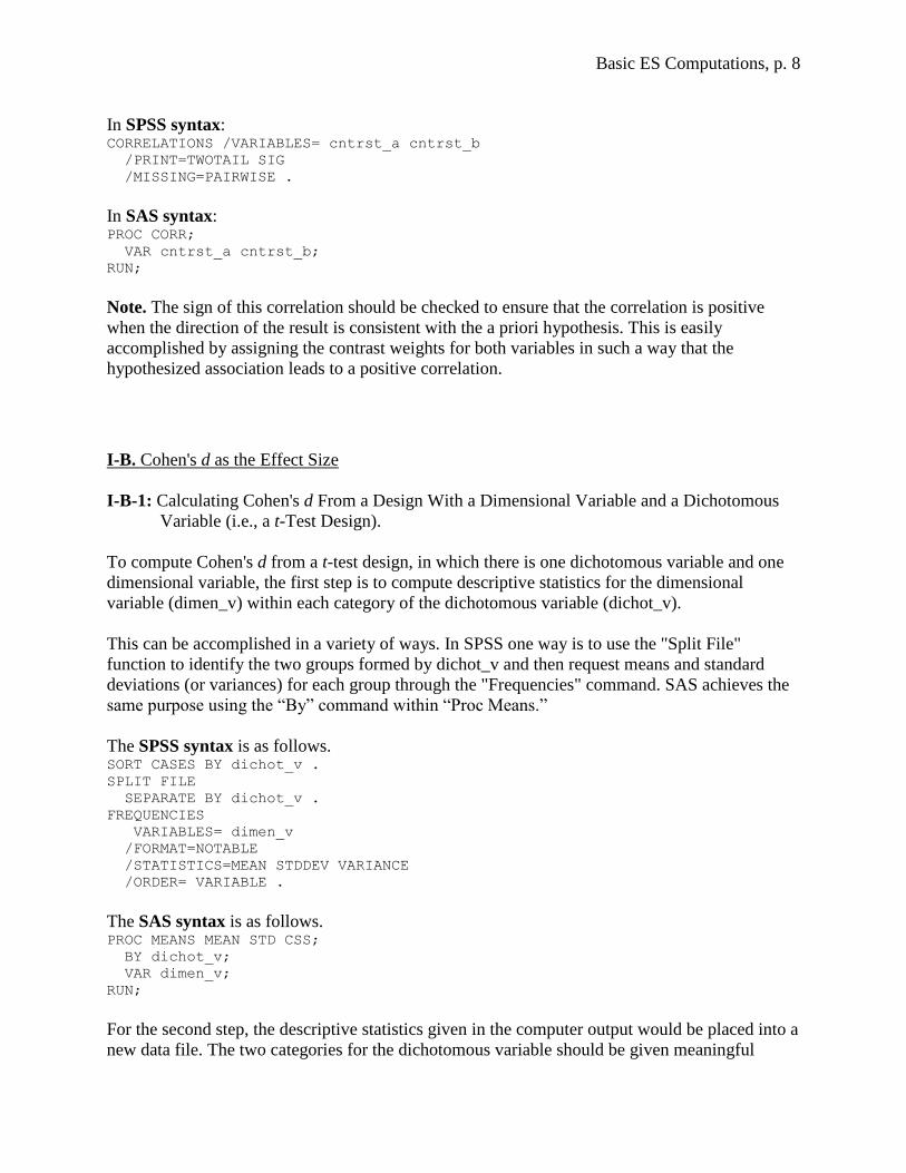
In SPSS syntax: CORRELATIONS /VARIABLES= cntrst_a cntrst_b
/PRINT=TWOTAIL SIG
/MISSING=PAIRWISE .
In SAS syntax: PROC CORR;
VAR cntrst_a cntrst_b;
RUN;
Note. The sign of this correlation should be checked to ensure that the correlation is positive
when the direction of the result is consistent with the a priori hypothesis. This is easily
accomplished by assigning the contrast weights for both variables in such a way that the
hypothesized association leads to a positive correlation.
I-B. Cohen's d as the Effect Size
I-B-1: Calculating Cohen's d From a Design With a Dimensional Variable and a Dichotomous
Variable (i.e., a t-Test Design).
To compute Cohen's d from a t-test design, in which there is one dichotomous variable and one
dimensional variable, the first step is to compute descriptive statistics for the dimensional
variable (dimen_v) within each category of the dichotomous variable (dichot_v).
This can be accomplished in a variety of ways. In SPSS one way is to use the "Split File"
function to identify the two groups formed by dichot_v and then request means and standard
deviations (or variances) for each group through the "Frequencies" command. SAS achieves the
same purpose using the “By” command within “Proc Means.”
The SPSS syntax is as follows. SORT CASES BY dichot_v .
SPLIT FILE
SEPARATE BY dichot_v .
FREQUENCIES
VARIABLES= dimen_v
/FORMAT=NOTABLE
/STATISTICS=MEAN STDDEV VARIANCE
/ORDER= VARIABLE .
The SAS syntax is as follows. PROC MEANS MEAN STD CSS;
BY dichot_v;
VAR dimen_v;
RUN;
For the second step, the descriptive statistics given in the computer output would be placed into a
new data file. The two categories for the dichotomous variable should be given meaningful

Basic ES Computations, p. 9
names, and in this example they will be referred to as grp1 and grp2 to designate group 1 and
group 2, respectively. Six pieces of information from the output file must be entered into the new
dataset.
If you are using SPSS, this information consists of the mean, SD, and valid N for the dimensional
variable in each group. Thus, for this example, six variable columns would be created in the new
data file and they would be labeled grp1Mean, grp1SD, grp1N, grp2Mean, grp2SD, and grp2N.
If you are using SAS, the six pieces of information consist of the mean, CSS, and valid N for the
dimensional variable in each group. The CSS, or corrected sum of squares, is the numerator of
the variance and dividing it by N produces the variance. Thus, for this example in SAS, the six
variable columns to create would be labeled grp1Mean, grp1CSS, grp1N, grp2Mean, grp2CSS,
and grp2N.
By default SPSS and SAS compute the SD as an inferential statistic (i.e., S) rather than as the
population parameter (i.e., ) by using N-1 in the denominator of the SD equation rather than N.
In order to obtain Cohen's d rather than Hedge's g, the inferential statistic S will be transformed
to through syntax.
After the relevant results have been entered into the new data file, syntax will be used to compute
the pooled variance (pool_Var), the pooled standard deviation (pool_SD), and then Cohen's d.
The syntax is as follows (where sqrt = square root, and **2 = squared).
SPSS: COMPUTE pool_var = (((grp1n - 1) * grp1sd**2) + ((grp2n - 1) * grp2sd**2)) /
(grp1n + grp2n) .
COMPUTE pool_sd = sqrt(pool_var).
COMPUTE Cohens_d = (grp1mean - grp2mean) / pool_sd .
EXECUTE .
SAS: DATA newdata;
SET olddata;
pool_var = (grp1css + grp2css) / (grp1n + grp2n);
pool_sd = sqrt(pool_var);
Cohens_d = (grp1mean - grp2mean) / pool_sd;
RUN;
Note. As a technical point, it may look like the SAS and SPSS syntax commands use different
procedures to compute the pooled variance. However, they do not. In both instances, the
descriptive variance (i.e., 2) for each group is weighted by sample size (i.e., n). In the case of
the SPSS syntax, two operations are being completed in a single step. The unbiased variance
estimate (i.e., S2) is being converted to the descriptive variance (i.e., 2) and also weighted by
sample size. The full formula to achieve this would be [n * (n-1)/n * S2] but it has been reduced
to its simplified form of [(n-1) * S2]. Similarly, in the case of the SAS syntax, because the CSS is
a raw sum of squares rather than a variance or SD the descriptive variance (i.e., 2) is computed
directly from CSS and weighted by sample size. The full formula would be [n * (CSS/n)] but this
was reduced to its simplified form, which is just CSS. In both the SPSS and SAS computations,
Basic ES Computations, p. 10
the final pooled 2 is obtained by dividing the sum of the weighted variances by the sum of the
weights.
Note. The sign of d is arbitrary. When the direction of the result is consistent with the a priori
hypothesis, it should be reported with a positive sign. When a result is in the direction opposite
of that specified by the hypothesis, it should be given a negative sign. This is easily
accomplished by designating the group that is expected to have the higher mean as group 1.
The steps listed above are somewhat complicated. Thus, until SPSS and SAS introduce a
command for generating Cohen's d, it is actually easier to compute Cohen's d after running a t-
test to compare mean differences across groups. The computations using this method are
described below in Section II-B-1.
Basic ES Computations, p. 11
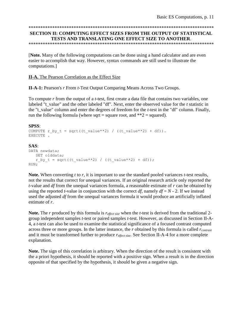
******************************************************************************
SECTION II: COMPUTING EFFECT SIZES FROM THE OUTPUT OF STATISTICAL
TESTS AND TRANSLATING ONE EFFECT SIZE TO ANOTHER.
******************************************************************************
[Note. Many of the following computations can be done using a hand calculator and are even
easier to accomplish that way. However, syntax commands are still used to illustrate the
computations.]
II-A. The Pearson Correlation as the Effect Size
II-A-1: Pearson's r From t-Test Output Comparing Means Across Two Groups.
To compute r from the output of a t-test, first create a data file that contains two variables, one
labeled "t_value" and the other labeled "df". Next, enter the observed value for the t statistic in
the "t_value" column and enter the degrees of freedom for the t-test in the "df" column. Finally,
run the following formula (where sqrt = square root, and **2 = squared).
SPSS: COMPUTE r_by_t = sqrt((t_value**2) / ((t_value**2) + df)).
EXECUTE .
SAS: DATA newdata;
SET olddata;
r_by_t = sqrt((t_value**2) / ((t_value**2) + df));
RUN;
Note. When converting t to r, it is important to use the standard pooled variances t-test results,
not the results that correct for unequal variances. If an original research article only reported the
t-value and df from the unequal variances formula, a reasonable estimate of r can be obtained by
using the reported t-value in conjunction with the correct df, namely df = N - 2. If we instead
used the adjusted df from the unequal variances formula it would produce an artificially inflated
estimate of r.
Note. The r produced by this formula is reffect size when the t-test is derived from the traditional 2-
group independent samples t-test or paired samples t-test. However, as discussed in Section II-A-
4, a t-test can also be used to examine the statistical significance of a focused contrast computed
across three or more groups. In the latter instance, the r obtained by this formula is called rcontrast
and it must be transformed further to produce reffect size. See Section II-A-4 for a more complete
explanation.
Note. The sign of this correlation is arbitrary. When the direction of the result is consistent with
the a priori hypothesis, it should be reported with a positive sign. When a result is in the direction
opposite of that specified by the hypothesis, it should be given a negative sign.
Basic ES Computations, p. 12
II-A-2: Pearson's r From 2 x 2 Chi-Square Output.
To compute r from a chi-square test with 1 degree of freedom (df) (i.e., from a 2 x 2 table), first
create a data file that contains two variables, one labeled "chisquar" and the other labeled "N".
Next, enter the observed value for the chi-square statistic in the "chisquar" column and enter the
total number of subjects for the analysis in the "N" column. Finally, run the following syntax
(where sqrt = square root).
SPSS: COMPUTE r_by_2x2 = sqrt(chisquar / N).
EXECUTE .
SAS: DATA newdata;
SET olddata;
r_by_2x2 = sqrt(chisquar / N);
RUN;
Note. The sign of this correlation is arbitrary. When the direction of the result is consistent with
the a priori hypothesis, it should be reported with a positive sign. When a result is in the direction
opposite of that specified by the hypothesis, it should be given a negative sign.
II-A-3. Pearson's r From F Test Output When Just Two Groups Have Been Compared.
To compute r from an F test with numerator df = 1, in which a dimensional variable has been
compared across just two groups (i.e., from a traditional t-test type of design), first create a data
file that contains two variables, one labeled "F_value" and the other labeled "df_wthin". Next,
enter the observed value for the F statistic in the "F_value" column and enter the within subjects
degrees of freedom for the F test in the "df_wthin" column (i.e., the denominator df). Finally, run
the following syntax (where sqrt = square root).
SPSS: COMPUTE r_by_f = sqrt(F_value / (F_value + df_wthin)).
EXECUTE .
SAS: DATA newdata;
SET olddata;
r_by_f = sqrt(F_value / (F_value + df_wthin));
RUN;
Note. The r produced by this formula is reffect size when the F test is derived from the comparison
of two independent samples. However, as discussed in Section II-A-4, an F test can also be used
to examine the statistical significance of a focused contrast computed across three or more
groups. In the latter instance, the resulting F is not conceptually equivalent to an F derived from
a 2-group comparison even though both F tests have 1 degree of freedom in the numerator. As
explained more completely in Section II-A-4, when more than two groups have been compared
via a focused contrast, the formula in this section produces rcontrast, which must be transformed
further to produce reffect size.

Basic ES Computations, p. 13
Note. The sign of this correlation is arbitrary. When the direction of the result is consistent with
the a priori hypothesis, it should be reported with a positive sign. When a result is in the direction
opposite of that specified by the hypothesis, it should be given a negative sign.
II-A-4: Pearson's r From F Test Output When More Than Two Groups Have Been Compared.
It is more complicated to compute r from the output of an F test in a traditional ANOVA design,
in which a dimensional variable has been compared across more than two groups (and it is not
possible to compute Cohen's d from data of this type). Because of the increased complexity,
example syntax for SPSS and SAS is not provided below. However, the procedures are described
in the following sources and they are summarized and illustrated here. The material that follows
presumes that readers are already familiar with previous sections in this document, particularly
the discussion of contrast weights in Sections I-A-3 and I-A-4.
Rosenthal, R., Rosnow, R. L., & Rubin, D. B. (2000). Contrasts and effect sizes in behavioral
research: A correlational approach. New York: Cambridge University Press.
Rosnow, R. L., & Rosenthal, R. (1996). Computing contrasts, effect sizes, and counternulls on
other people's published data: General procedures for research consumers. Psychological
Methods, 1, 331-340.
Rosnow, R. L., Rosenthal, R., & Rubin, D. B. (2000). Contrasts and correlations in effect-size
estimation. Psychological Science, 11, 446-453.
The complexity of computing reffect size from the output of a traditional ANOVA arises from two
main factors. First, obtaining the final coefficient requires multiple computational steps. Second,
complexity arises from the fact that r can be computed from different kinds of incompletely
reported initial information. Because ANOVA results in the published literature may report
different types of incomplete information, the latter provides secondary researchers with some
flexibility when they wish to compute reffect size from studies conducted by other people.
Several approaches to computing r will be explained and illustrated here. Each scenario makes
uses of slightly different pieces of initial information. However, for simplicity, the same example
data set is used throughout. The data set is described in Rosnow and Rosenthal (1996).
II-A-4-a: Scenario 1 - When given group Ms and F or t from a focused contrast
Scenario 1 is applicable when the original output provides
a) the mean for the dimensional variable in each of the multi-category groups and
b) the t-value or F-value that comes from testing a focused contrast across the multi-
category variable.
This is a basic scenario, although it is not likely to be encountered often because authors
typically have computed omnibus F tests rather than focused contrasts. An omnibus F test
determines whether there is any pattern in the means that is unlikely to be due to chance, while a
focused contrast determines whether there is a specified and expected pattern in the means that is
Basic ES Computations, p. 14
unlikely to be due to chance. A meaningful effect size can be obtained from the latter but not the
former.
Note. Either a t-test or an F test can be used to evaluate a multi-group focused contrast. These
statistics are psychometrically equivalent because F = t2. For instance, a researcher wishing to
produce a focused contrast in SPSS would use the One-way ANOVA procedure and would
specify contrast weight coefficients on the "/CONTRAST" subcommand. The statistical output
from this set of commands would be in the form of a t-test rather than an F test.
Assuming an existing study provides mean scores across all groups and t or F from a focused
contrast we can compute reffect size in three steps. First, the t or F is converted to rcontrast. Second,
the coefficient called ralerting is computed. Third, rcontrast and ralerting are used to produce reffect size.
For the first step, use the formulas from Sections II-A-1 (for t-test output) or II-A-3 (for F test
output) to translate the results of the statistical test into an initial r. Previously, the formulas in
Sections II-A-1 and II-A-3 were used to compute reffect size directly from the t or F output. This
was possible because the statistical results had been obtained by comparing means across just
two groups. However, when t or F are obtained from a focused contrast that compares means
across three or more groups, the r produced by these formulas is no longer equivalent to reffect size.
Instead, the r is known as rcontrast to indicate that it is derived from a multi-group contrast.
The definition of rcontrast is somewhat difficult to grasp. Fortunately, a complete understanding is
not essential to follow the procedures outlined here. Nonetheless, rcontrast is defined as the
correlation between each individual's classification on the multi-category variable and his or her
score on the dimensional variable AFTER partialing out between group variability that is not due
to the focused contrast.
For the second step in our efforts to produce reffect size we need to compute ralerting, which is the
correlation between each group's mean score on the dimensional variable and the contrast weight
assigned to that group. Thus, if there are three groups with means of 2.0, 3.5, and 5.0 and the
groups have been assigned contrast weights of -1, 0, and 1, then these three pairs of values (i.e.,
2.0 and -1; 3.5 and 0; and 5.0 and 1) are correlated to produce ralerting = 1.0.
For the third and final step, the results from the first two steps are entered into the following
formula to compute reffect size. (Note that both rcontrast and ralerting are squared in the denominator of
the equation.)
reffect size = rcontrast / square root[(1 - r2contrast) + (r2
contrast / r2
alerting)]
To illustrate these procedures, suppose a researcher hypothesizes higher doses of anti-anxiety
medication will lead to increased functioning in patients with anxiety disorders. The researcher
randomly assigns 20 patients to four groups that differ in medication dose, including no
medication, 100 milligrams, 200 mg, and 300 mg. Given these four conditions and the stated
hypothesis that mean scores of functioning should increase in tandem with increasing medication
dosage, appropriate contrast weights are assigned to the four groups to test a focused hypothesis.
In this instance, appropriate contrast weights would be -3, -1, +1, and +3, respectively. These
weights sum to zero and they indicate that the group means should be ordered as follows: no
Basic ES Computations, p. 15
medication < 100 mg < 200 mg < 300 mg. Let's assume that besides this information (i.e., that
there are four groups and a logical hypothesis that dictates appropriate contrast weights) the only
data available from the researcher's original report are the results of an F test examining the
contrast hypothesis and the mean score on the functioning variable in each group after treatment.
Specifically, we know:
Fcontrast(1,16) = 100.0, and
Condition Mean Post-
Treatment
Contrast
Weight
No medication 3.0 -3
100 mg 1.0 -1
200 mg 9.0 +1
300 mg 7.0 +3
Note that by definition, F = t2. Thus, when Fcontrast(1,16) = 100.0, tcontrast(16) = 10.0. Given this,
we can use either the formula in Section II-A-1 (for t) or in Section II-A-3 (for F) to translate the
results into rcontrast. For simplicity, we will use the equation from Section II-A-3:
rcontrast = square root(F / (F + dfwithin))
= square root(100 / (100 + 16))
= square root(.86)
= .928
Next, we compute ralerting by correlating the values in the Post Treatment Mean column of the
table above with the values in the Contrast Weights column. Doing so we find ralerting = .707.
Finally, we use rcontrast and ralerting to obtain reffect size. Using the example data, the equation would
be:
reffect size = rcontrast / square root[(1 - r2contrast) + (r2
contrast / r2
alerting)]
= .928 / square root[(1 - .861) + (.861 / .500)]
= .928 / square root(1.861)
= .928 / 1.364
= .680
Thus, the researcher's focused hypothesis was supported. The impact of increasing dosages of
anti-anxiety medication on improved functioning in patients with anxiety disorders is reffect size =
.68, which is a substantial effect.
II-A-4-b: Scenario 2 - When given group Ms, SDs, and ns
Scenario 2 is applicable when the original output provides
a) the mean for the dimensional variable in each of the multi-category groups,
b) the SD for the dimensional variable in each group, and
c) the n in each group.
Basic ES Computations, p. 16
Most often, findings in the published literature do not report F-tests derived from a focused
contrast. A more common scenario occurs when the original report provides the mean, the SD,
and the n for the dimensional variable in each of the multi-category groups. Using this
information, we can compute reffect size in a 4-step process. First, we compute a t test that evaluates
the relevant focused contrast, known as tcontrast. This is the hard part. With this value in hand, we
simply follow the remaining steps that had been outlined under Scenario 1. Thus, step two
converts tcontrast to rcontrast, step three computes ralerting, and step four uses rcontrast and ralerting to
obtain reffect size.
As mentioned, the hard part is computing a t-value that corresponds to the focused contrast. This
is accomplished through a formula provided in Rosnow and Rosenthal (1996; Equation 1) or
Rosenthal et al. (2000; Equation 3.10). This formula is somewhat difficult to reproduce in a text
file that will be converted by various word processing programs. However, it is provided below
in a somewhat longhand form.
tcontrast = Summation(Mi * CWi) / square root[MSwithin * (Summation(CW2i / ni))]
where Mi is the mean for each group, CWi is the contrast weight assigned to each group, ni is the
number of subjects in each group, and MSwithin is the error variance from a between subjects
ANOVA. The MSwithin can also be estimated by computing the pooled variance across groups,
with each variance weighted by sample size; i.e., [Summation(SD2i * ni) / N].
To illustrate this formula, we again use the example begun in Scenario 1. As before, the
hypothesis is that functioning should increase as medication dosage increases. Although the
original research report may not have specified appropriate contrast weights, the hypothesis
dictates the appropriate contrast weights that we should assign to the four medication groups.
Let's assume that this time the research report provided group Ms, SDs and ns, but did not
provide the results from an F test examining a focused hypothesis. Consequently, the available
information consists of group data and a logical hypothesis that we use to produce contrast
weights. The information is as follows:
Condition Post Treatment Contrast
Weight Mean SD n
No medication 3.0 1.0 5 -3
100 mg 1.0 1.0 5 -1
200 mg 9.0 1.0 5 +1
300 mg 7.0 1.0 5 +3
With these pieces of data, the first step is to compute tcontrast. However, to do so we also need the
MSwithin. Because the research report did not provide this information, we will estimate it using
the pooled variance across groups. Because each group has SD = 1 and n = 5, some readers may
realize immediately that the pooled variance will be 1.0. However, for the sake of clarity, the
computations will be illustrated across the four groups using the equation Summation(SD2i * ni) /
N, where i = groups 1 to 4.
Basic ES Computations, p. 17
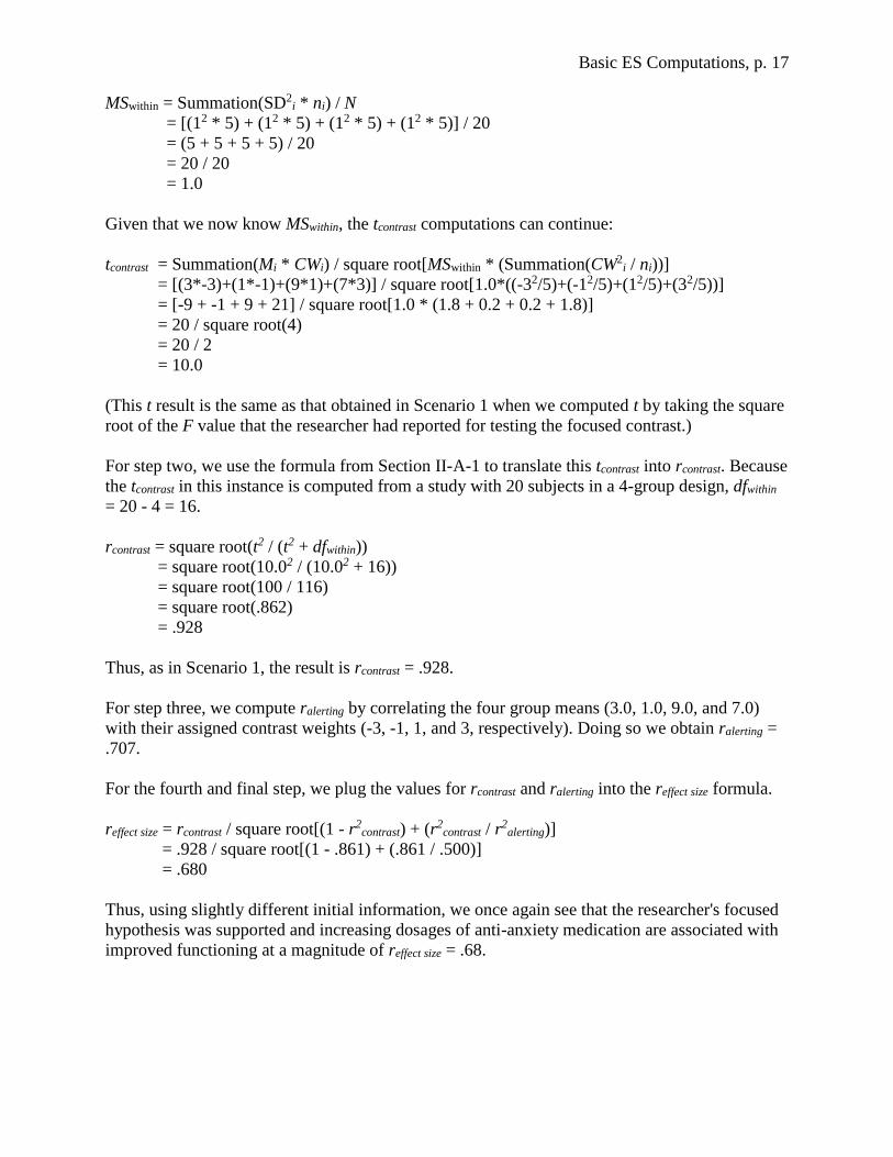
MSwithin = Summation(SD2i * ni) / N
= [(12 * 5) + (12 * 5) + (12 * 5) + (12 * 5)] / 20
= (5 + 5 + 5 + 5) / 20
= 20 / 20
= 1.0
Given that we now know MSwithin, the tcontrast computations can continue:
tcontrast = Summation(Mi * CWi) / square root[MSwithin * (Summation(CW2i / ni))]
= [(3*-3)+(1*-1)+(9*1)+(7*3)] / square root[1.0*((-32/5)+(-12/5)+(12/5)+(32/5))]
= [-9 + -1 + 9 + 21] / square root[1.0 * (1.8 + 0.2 + 0.2 + 1.8)]
= 20 / square root(4)
= 20 / 2
= 10.0
(This t result is the same as that obtained in Scenario 1 when we computed t by taking the square
root of the F value that the researcher had reported for testing the focused contrast.)
For step two, we use the formula from Section II-A-1 to translate this tcontrast into rcontrast. Because
the tcontrast in this instance is computed from a study with 20 subjects in a 4-group design, dfwithin
= 20 - 4 = 16.
rcontrast = square root(t2 / (t2 + dfwithin))
= square root(10.02 / (10.02 + 16))
= square root(100 / 116)
= square root(.862)
= .928
Thus, as in Scenario 1, the result is rcontrast = .928.
For step three, we compute ralerting by correlating the four group means (3.0, 1.0, 9.0, and 7.0)
with their assigned contrast weights (-3, -1, 1, and 3, respectively). Doing so we obtain ralerting =
.707.
For the fourth and final step, we plug the values for rcontrast and ralerting into the reffect size formula.
reffect size = rcontrast / square root[(1 - r2contrast) + (r2
contrast / r2
alerting)]
= .928 / square root[(1 - .861) + (.861 / .500)]
= .680
Thus, using slightly different initial information, we once again see that the researcher's focused
hypothesis was supported and increasing dosages of anti-anxiety medication are associated with
improved functioning at a magnitude of reffect size = .68.
Basic ES Computations, p. 18
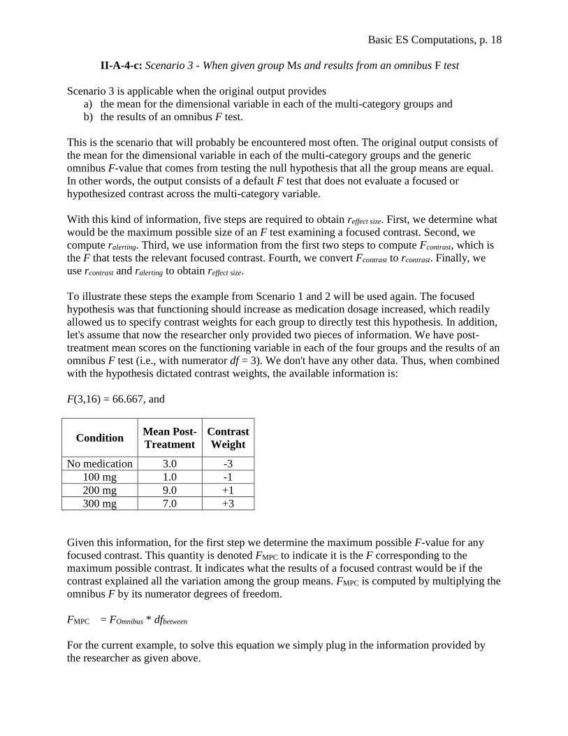
II-A-4-c: Scenario 3 - When given group Ms and results from an omnibus F test
Scenario 3 is applicable when the original output provides
a) the mean for the dimensional variable in each of the multi-category groups and
b) the results of an omnibus F test.
This is the scenario that will probably be encountered most often. The original output consists of
the mean for the dimensional variable in each of the multi-category groups and the generic
omnibus F-value that comes from testing the null hypothesis that all the group means are equal.
In other words, the output consists of a default F test that does not evaluate a focused or
hypothesized contrast across the multi-category variable.
With this kind of information, five steps are required to obtain reffect size. First, we determine what
would be the maximum possible size of an F test examining a focused contrast. Second, we
compute ralerting. Third, we use information from the first two steps to compute Fcontrast, which is
the F that tests the relevant focused contrast. Fourth, we convert Fcontrast to rcontrast. Finally, we
use rcontrast and ralerting to obtain reffect size.
To illustrate these steps the example from Scenario 1 and 2 will be used again. The focused
hypothesis was that functioning should increase as medication dosage increased, which readily
allowed us to specify contrast weights for each group to directly test this hypothesis. In addition,
let's assume that now the researcher only provided two pieces of information. We have post-
treatment mean scores on the functioning variable in each of the four groups and the results of an
omnibus F test (i.e., with numerator df = 3). We don't have any other data. Thus, when combined
with the hypothesis dictated contrast weights, the available information is:
F(3,16) = 66.667, and
Condition Mean Post-
Treatment
Contrast
Weight
No medication 3.0 -3
100 mg 1.0 -1
200 mg 9.0 +1
300 mg 7.0 +3
Given this information, for the first step we determine the maximum possible F-value for any
focused contrast. This quantity is denoted FMPC to indicate it is the F corresponding to the
maximum possible contrast. It indicates what the results of a focused contrast would be if the
contrast explained all the variation among the group means. FMPC is computed by multiplying the
omnibus F by its numerator degrees of freedom.
FMPC = FOmnibus * dfbetween
For the current example, to solve this equation we simply plug in the information provided by
the researcher as given above.
Basic ES Computations, p. 19
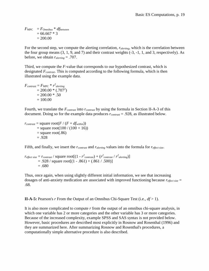
FMPC = FOmnibus * dfbetween
= 66.667 * 3
= 200.00
For the second step, we compute the alerting correlation, ralerting, which is the correlation between
the four group means (3, 1, 9, and 7) and their contrast weights (-3, -1, 1, and 3, respectively). As
before, we obtain ralerting = .707.
Third, we compute the F-value that corresponds to our hypothesized contrast, which is
designated Fcontrast. This is computed according to the following formula, which is then
illustrated using the example data.
Fcontrast = FMPC * r2alerting
= 200.00 * (.7072)
= 200.00 * .50
= 100.00
Fourth, we translate the Fcontrast into rcontrast by using the formula in Section II-A-3 of this
document. Doing so for the example data produces rcontrast = .928, as illustrated below.
rcontrast = square root(F / (F + dfwithin))
= square root(100 / (100 + 16))
= square root(.86)
= .928
Fifth, and finally, we insert the rcontrast and ralerting values into the formula for reffect size.
reffect size = rcontrast / square root[(1 - r2contrast) + (r2
contrast / r2
alerting)]
= .928 / square root[(1 - .861) + (.861 / .500)]
= .680
Thus, once again, when using slightly different initial information, we see that increasing
dosages of anti-anxiety medication are associated with improved functioning because reffect size =
.68.
II-A-5: Pearson's r From the Output of an Omnibus Chi-Square Test (i.e., df > 1).
It is also more complicated to compute r from the output of an omnibus chi-square analysis, in
which one variable has 2 or more categories and the other variable has 3 or more categories.
Because of the increased complexity, example SPSS and SAS syntax is not provided below.
However, basic procedures are described most explicitly in Rosnow and Rosenthal (1996) and
they are summarized here. After summarizing Rosnow and Rosenthal's procedures, a
computationally simple alternative procedure is also described.
Basic ES Computations, p. 20
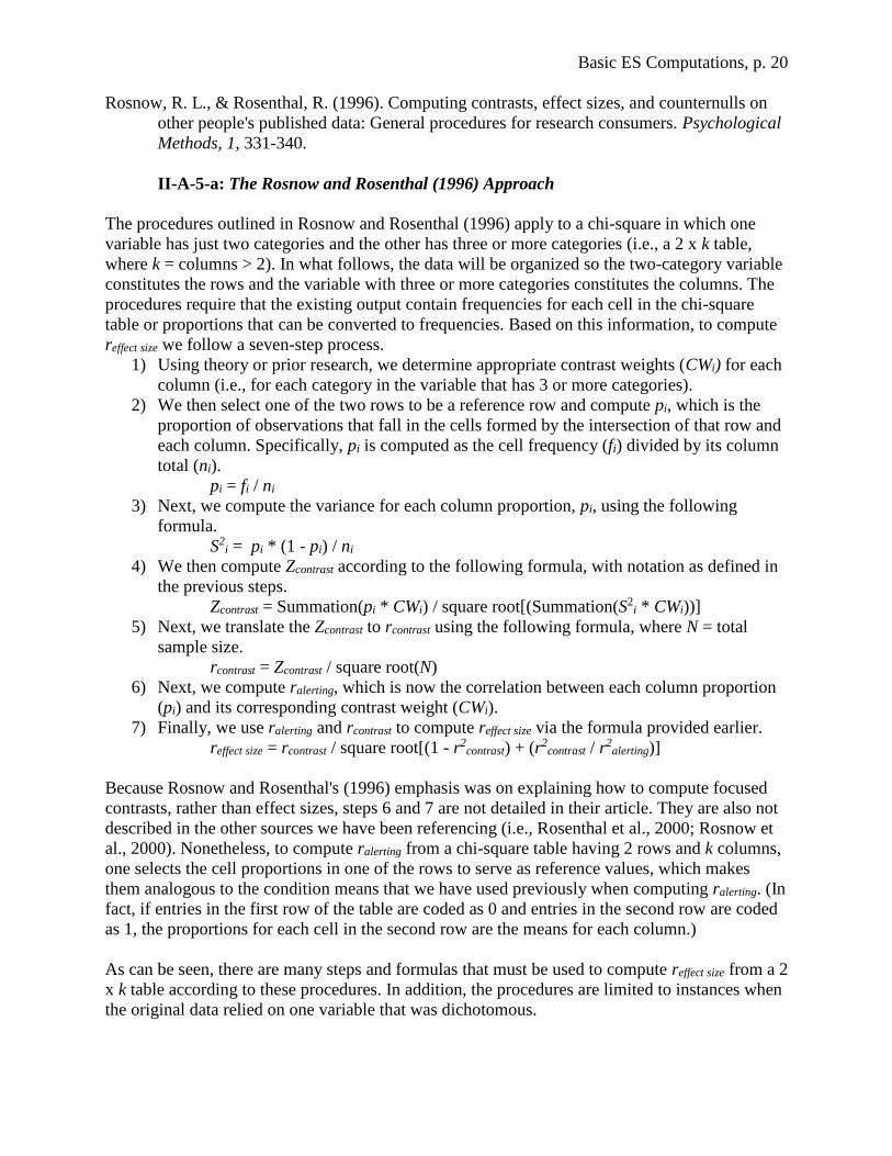
Rosnow, R. L., & Rosenthal, R. (1996). Computing contrasts, effect sizes, and counternulls on
other people's published data: General procedures for research consumers. Psychological
Methods, 1, 331-340.
II-A-5-a: The Rosnow and Rosenthal (1996) Approach
The procedures outlined in Rosnow and Rosenthal (1996) apply to a chi-square in which one
variable has just two categories and the other has three or more categories (i.e., a 2 x k table,
where k = columns > 2). In what follows, the data will be organized so the two-category variable
constitutes the rows and the variable with three or more categories constitutes the columns. The
procedures require that the existing output contain frequencies for each cell in the chi-square
table or proportions that can be converted to frequencies. Based on this information, to compute
reffect size we follow a seven-step process.
1) Using theory or prior research, we determine appropriate contrast weights (CWi) for each
column (i.e., for each category in the variable that has 3 or more categories).
2) We then select one of the two rows to be a reference row and compute pi, which is the
proportion of observations that fall in the cells formed by the intersection of that row and
each column. Specifically, pi is computed as the cell frequency (fi) divided by its column
total (ni).
pi = fi / ni
3) Next, we compute the variance for each column proportion, pi, using the following
formula.
S2i = pi * (1 - pi) / ni
4) We then compute Zcontrast according to the following formula, with notation as defined in
the previous steps.
Zcontrast = Summation(pi * CWi) / square root[(Summation(S2i * CWi))]
5) Next, we translate the Zcontrast to rcontrast using the following formula, where N = total
sample size.
rcontrast = Zcontrast / square root(N)
6) Next, we compute ralerting, which is now the correlation between each column proportion
(pi) and its corresponding contrast weight (CWi).
7) Finally, we use ralerting and rcontrast to compute reffect size via the formula provided earlier.
reffect size = rcontrast / square root[(1 - r2contrast) + (r2
contrast / r2
alerting)]
Because Rosnow and Rosenthal's (1996) emphasis was on explaining how to compute focused
contrasts, rather than effect sizes, steps 6 and 7 are not detailed in their article. They are also not
described in the other sources we have been referencing (i.e., Rosenthal et al., 2000; Rosnow et
al., 2000). Nonetheless, to compute ralerting from a chi-square table having 2 rows and k columns,
one selects the cell proportions in one of the rows to serve as reference values, which makes
them analogous to the condition means that we have used previously when computing ralerting. (In
fact, if entries in the first row of the table are coded as 0 and entries in the second row are coded
as 1, the proportions for each cell in the second row are the means for each column.)
As can be seen, there are many steps and formulas that must be used to compute reffect size from a 2
x k table according to these procedures. In addition, the procedures are limited to instances when
the original data relied on one variable that was dichotomous.

Basic ES Computations, p. 21
To contend with these limitations, there is an alternative set of procedures that can be employed.
These procedures also require frequency information for each cell in a chi-square table (or the
ability to compute frequency information from proportions or other data). However, one benefit
of the alternative procedures is that they are not limited to a 2 x k design and instead can be
employed with tables of any size. In addition, the procedures do not require the use of any
formulas, though they do require some data entry.
II-A-5-b: Reconstructing the database
For the alternative procedures, the goal is to reconstruct a version of the original database. To do
so, we need cell frequencies for the table (or some means of computing the frequencies) and we
need to be able to specify an appropriate hypothesized contrast for both variables in the chi-
square analysis.
With this information, the only remaining step is to re-create a version of the original database.
When doing this, each subject in the data set is assigned two values, one corresponding to their
row contrast weight and the other corresponding to their column contrast weight. In other words,
we create a new data set that assigns appropriate contrast weights for both variables to each
"subject" in the original study.
For instance, let's assume the design is a 3 x 3 table in which 3 categories of MMPI-2 T-scores
on Scale 2 are examined in relation to a 3-category classification of depressive disorders. (Note
that MMPI-2 scores would most appropriately be analyzed as dimensional variables rather than
being split into three categories. The latter is done here simply to illustrate the procedures.)
MMPI-2 T-Scores are classified as below average (i.e., T < 50), average to mildly elevated (i.e.,
T = 50 to 65), and moderately to severely elevated (i.e., T > 65). The three categories of
depressive disorder diagnoses are classified as No Depressive Diagnosis, Dysthymia, and Major
Depression. The research hypothesis is that higher elevations on Scale 2 are positively associated
with more severe depressive diagnoses.
In this instance, appropriate MMPI-2 Scale 2 contrast weights would be formed by assigning a
value of -1 to subjects with T-Scores < 50, a value of 0 to subjects with T-Scores in the range
between 50 and 65, and a value of 1 to subjects with T-Scores > 65. For the diagnosis variable,
the appropriate contrast weights would be: no depressive diagnosis = -1, dysthymia = 0, and
major depression = 1.
Next, we create a new data set in SPSS or SAS. The data set will consist of two variable columns
(a third optional column can also be used to indicate subject ID numbers). The first variable
column will be used to record the contrast weights for the MMPI-2 Scale 2 classifications and
the other variable column will be used to record the contrast weights for the depressive disorder
classifications.
After the dataset structure is created the next step is to systematically translate the chi-square
table of cell frequencies into the new data set. Let's assume that the existing table is set up as a 3
x 3 matrix of cell frequencies, as depicted below. (If the table of frequencies does not exist in this
form but can be produced from other information, our initial effort would be to create the 3 x 3
matrix of frequencies.) Our first step is to add notations to the table that designate the appropriate
Basic ES Computations, p. 22
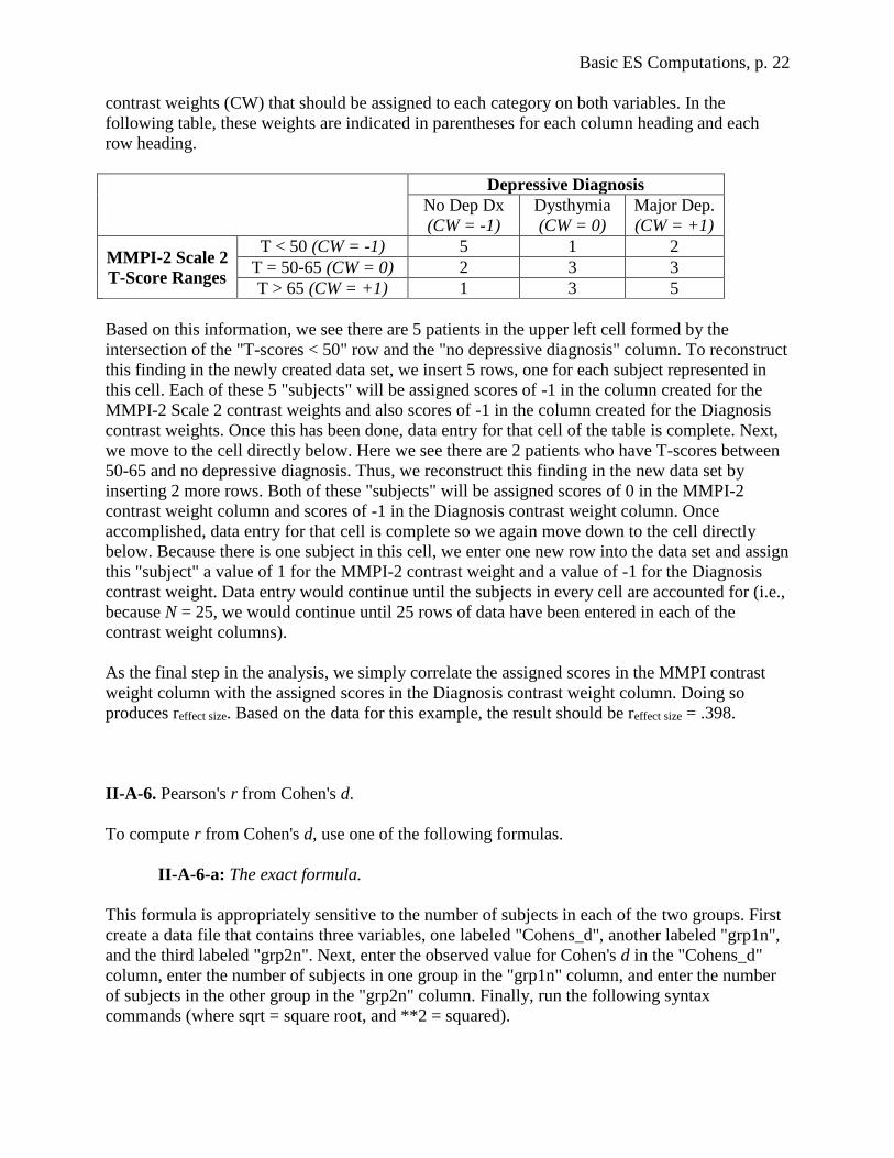
contrast weights (CW) that should be assigned to each category on both variables. In the
following table, these weights are indicated in parentheses for each column heading and each
row heading.
Depressive Diagnosis
No Dep Dx
(CW = -1)
Dysthymia
(CW = 0)
Major Dep.
(CW = +1)
MMPI-2 Scale 2
T-Score Ranges
T < 50 (CW = -1) 5 1 2
T = 50-65 (CW = 0) 2 3 3
T > 65 (CW = +1) 1 3 5
Based on this information, we see there are 5 patients in the upper left cell formed by the
intersection of the "T-scores < 50" row and the "no depressive diagnosis" column. To reconstruct
this finding in the newly created data set, we insert 5 rows, one for each subject represented in
this cell. Each of these 5 "subjects" will be assigned scores of -1 in the column created for the
MMPI-2 Scale 2 contrast weights and also scores of -1 in the column created for the Diagnosis
contrast weights. Once this has been done, data entry for that cell of the table is complete. Next,
we move to the cell directly below. Here we see there are 2 patients who have T-scores between
50-65 and no depressive diagnosis. Thus, we reconstruct this finding in the new data set by
inserting 2 more rows. Both of these "subjects" will be assigned scores of 0 in the MMPI-2
contrast weight column and scores of -1 in the Diagnosis contrast weight column. Once
accomplished, data entry for that cell is complete so we again move down to the cell directly
below. Because there is one subject in this cell, we enter one new row into the data set and assign
this "subject" a value of 1 for the MMPI-2 contrast weight and a value of -1 for the Diagnosis
contrast weight. Data entry would continue until the subjects in every cell are accounted for (i.e.,
because N = 25, we would continue until 25 rows of data have been entered in each of the
contrast weight columns).
As the final step in the analysis, we simply correlate the assigned scores in the MMPI contrast
weight column with the assigned scores in the Diagnosis contrast weight column. Doing so
produces reffect size. Based on the data for this example, the result should be reffect size = .398.
II-A-6. Pearson's r from Cohen's d.
To compute r from Cohen's d, use one of the following formulas.
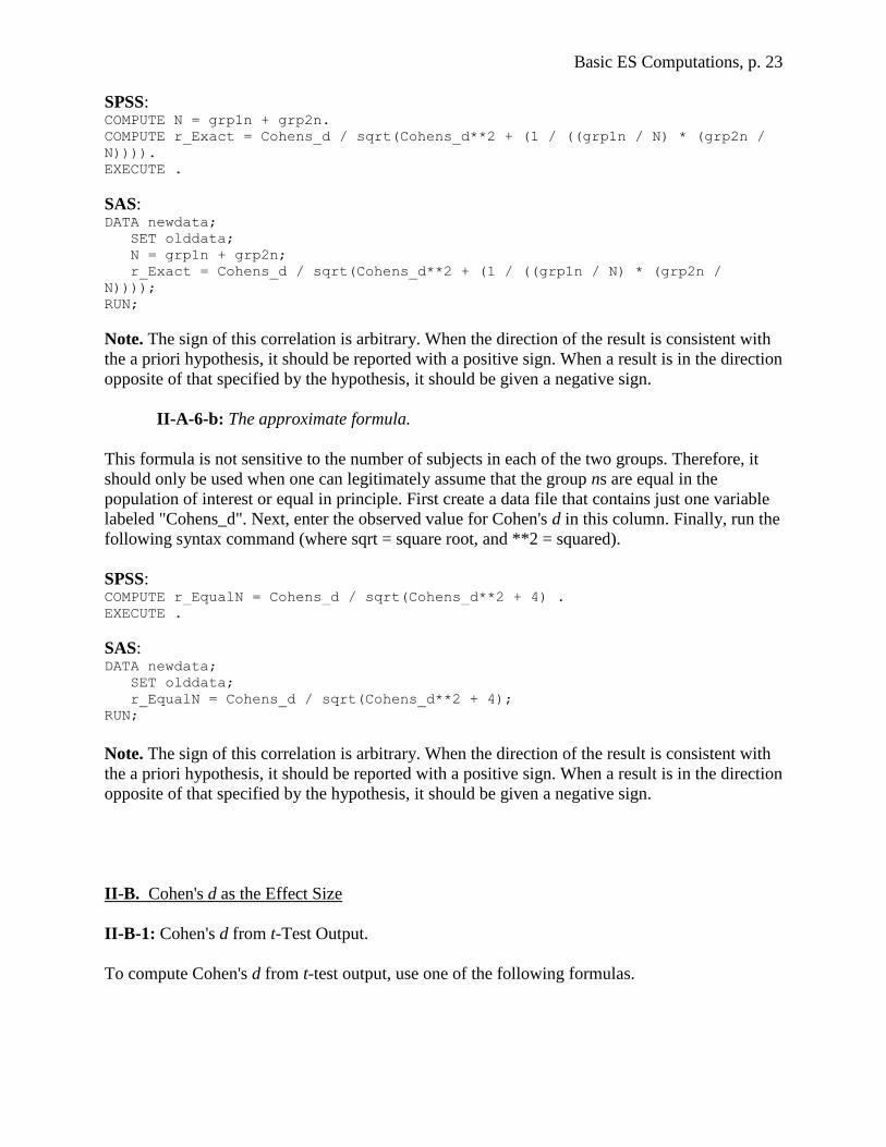
II-A-6-a: The exact formula.
This formula is appropriately sensitive to the number of subjects in each of the two groups. First
create a data file that contains three variables, one labeled "Cohens_d", another labeled "grp1n",
and the third labeled "grp2n". Next, enter the observed value for Cohen's d in the "Cohens_d"
column, enter the number of subjects in one group in the "grp1n" column, and enter the number
of subjects in the other group in the "grp2n" column. Finally, run the following syntax
commands (where sqrt = square root, and **2 = squared).
Basic ES Computations, p. 23
SPSS: COMPUTE N = grp1n + grp2n.
COMPUTE r_Exact = Cohens_d / sqrt(Cohens_d**2 + (1 / ((grp1n / N) * (grp2n /
N)))).
EXECUTE .
SAS: DATA newdata;
SET olddata;
N = grp1n + grp2n;
r_Exact = Cohens_d / sqrt(Cohens_d**2 + (1 / ((grp1n / N) * (grp2n /
N))));
RUN;
Note. The sign of this correlation is arbitrary. When the direction of the result is consistent with
the a priori hypothesis, it should be reported with a positive sign. When a result is in the direction
opposite of that specified by the hypothesis, it should be given a negative sign.
II-A-6-b: The approximate formula.
This formula is not sensitive to the number of subjects in each of the two groups. Therefore, it
should only be used when one can legitimately assume that the group ns are equal in the
population of interest or equal in principle. First create a data file that contains just one variable
labeled "Cohens_d". Next, enter the observed value for Cohen's d in this column. Finally, run the
following syntax command (where sqrt = square root, and **2 = squared).
SPSS: COMPUTE r_EqualN = Cohens_d / sqrt(Cohens_d**2 + 4) .
EXECUTE .
SAS: DATA newdata;
SET olddata;
r_EqualN = Cohens_d / sqrt(Cohens_d**2 + 4);
RUN;
Note. The sign of this correlation is arbitrary. When the direction of the result is consistent with
the a priori hypothesis, it should be reported with a positive sign. When a result is in the direction
opposite of that specified by the hypothesis, it should be given a negative sign.
II-B. Cohen's d as the Effect Size
II-B-1: Cohen's d from t-Test Output.
To compute Cohen's d from t-test output, use one of the following formulas.
Basic ES Computations, p. 24
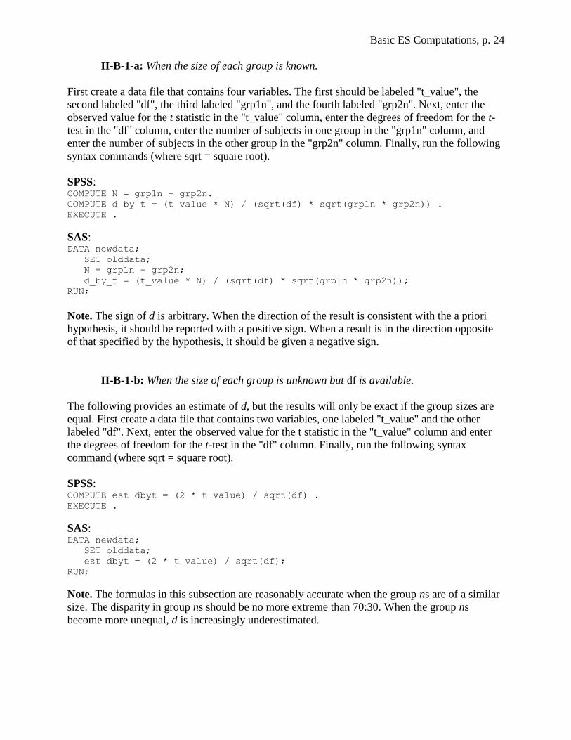
II-B-1-a: When the size of each group is known.
First create a data file that contains four variables. The first should be labeled "t_value", the
second labeled "df", the third labeled "grp1n", and the fourth labeled "grp2n". Next, enter the
observed value for the t statistic in the "t_value" column, enter the degrees of freedom for the t-
test in the "df" column, enter the number of subjects in one group in the "grp1n" column, and
enter the number of subjects in the other group in the "grp2n" column. Finally, run the following
syntax commands (where sqrt = square root).
SPSS: COMPUTE N = grp1n + grp2n.
COMPUTE d_by_t = (t_value * N) / (sqrt(df) * sqrt(grp1n * grp2n)) .
EXECUTE .
SAS: DATA newdata;
SET olddata;
N = grp1n + grp2n;
d_by_t = (t_value * N) / (sqrt(df) * sqrt(grp1n * grp2n));
RUN;
Note. The sign of d is arbitrary. When the direction of the result is consistent with the a priori
hypothesis, it should be reported with a positive sign. When a result is in the direction opposite
of that specified by the hypothesis, it should be given a negative sign.
II-B-1-b: When the size of each group is unknown but df is available.
The following provides an estimate of d, but the results will only be exact if the group sizes are
equal. First create a data file that contains two variables, one labeled "t_value" and the other
labeled "df". Next, enter the observed value for the t statistic in the "t_value" column and enter
the degrees of freedom for the t-test in the "df" column. Finally, run the following syntax
command (where sqrt = square root).
SPSS: COMPUTE est_dbyt = (2 * t_value) / sqrt(df) .
EXECUTE .
SAS: DATA newdata;
SET olddata;
est_dbyt = (2 * t_value) / sqrt(df);
RUN;
Note. The formulas in this subsection are reasonably accurate when the group ns are of a similar
size. The disparity in group ns should be no more extreme than 70:30. When the group ns
become more unequal, d is increasingly underestimated.
Basic ES Computations, p. 25
Note. The sign of d is arbitrary. When the direction of the result is consistent with the a priori
hypothesis, it should be reported with a positive sign. When a result is in the direction opposite
of that specified by the hypothesis, it should be given a negative sign.
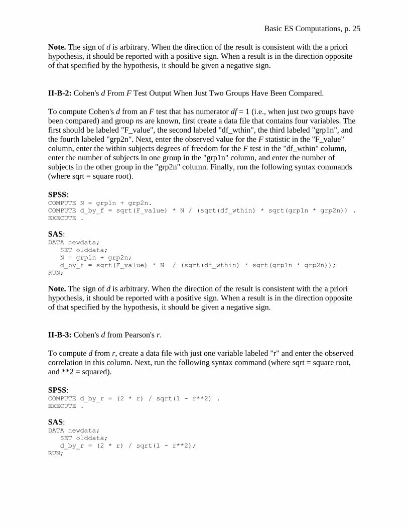
II-B-2: Cohen's d From F Test Output When Just Two Groups Have Been Compared.
To compute Cohen's d from an F test that has numerator df = 1 (i.e., when just two groups have
been compared) and group ns are known, first create a data file that contains four variables. The
first should be labeled "F_value", the second labeled "df_wthin", the third labeled "grp1n", and
the fourth labeled "grp2n". Next, enter the observed value for the F statistic in the "F_value"
column, enter the within subjects degrees of freedom for the F test in the "df_wthin" column,
enter the number of subjects in one group in the "grp1n" column, and enter the number of
subjects in the other group in the "grp2n" column. Finally, run the following syntax commands
(where sqrt = square root).
SPSS: COMPUTE N = grp1n + grp2n.
COMPUTE d_by_f = sqrt(F_value) * N / (sqrt(df_wthin) * sqrt(grp1n * grp2n)) .
EXECUTE .
SAS: DATA newdata;
SET olddata;
N = grp1n + grp2n;
d_by_f = sqrt(F_value) * N / (sqrt(df_wthin) * sqrt(grp1n * grp2n));
RUN;
Note. The sign of d is arbitrary. When the direction of the result is consistent with the a priori
hypothesis, it should be reported with a positive sign. When a result is in the direction opposite
of that specified by the hypothesis, it should be given a negative sign.
II-B-3: Cohen's d from Pearson's r.
To compute d from r, create a data file with just one variable labeled "r" and enter the observed
correlation in this column. Next, run the following syntax command (where sqrt = square root,
and **2 = squared).
SPSS: COMPUTE d_by_r = (2 * r) / sqrt(1 - r**2) .
EXECUTE .
SAS: DATA newdata;
SET olddata;
d_by_r = (2 * r) / sqrt(1 - r**2);
RUN;
Basic ES Computations, p. 26
Note. Transformations from r to d and vice versa are imprecise because r is sensitive to marginal
distributions (i.e., the number of subjects in each category of a dichotomous variable) but
generally speaking Cohen's d is not.
Note. The sign of d is arbitrary. When the direction of the result is consistent with the a priori
hypothesis, it should be reported with a positive sign. When a result is in the direction opposite
of that specified by the hypothesis, it should be given a negative sign.
****************************************************************************
All formulas in this document were obtained from one of the following sources:
Rosenthal, R. (1991). Meta-analytic procedures for social research (revised). Newbury Park,
CA: Sage.
Rosenthal, R., Rosnow, R. L., & Rubin, D. B. (2000). Contrasts and effect sizes in behavioral
research: A correlational approach. New York: Cambridge University Press.
Rosnow, R. L., & Rosenthal, R. (1996). Computing contrasts, effect sizes, and counternulls on
other people's published data: General procedures for research consumers. Psychological
Methods, 1, 331-340.
Rosnow, R. L., Rosenthal, R., & Rubin, D. B. (2000). Contrasts and correlations in effect-size
estimation. Psychological Science, 11, 446-453.
****************************************************************************