CLASSICAL ALGEBRAIC GEOMETRY Daniel PlaumannUniversität Konstanz

Summer ����

�. CURVES

� .� . D����� ��� �����

Let X ⊂ Pn be an irreducible curve of degree d. We know that the Hilbert poly-nomial pX is a polynomial of degree � with rational coe�cients. As such, it providesus with two numbers: We know that the leading coe�cient of pX is the degree of X.�e meaning of the constant term pX(�) is less clear. Note �rst that this is always aninteger (see Exercise ��.�).

De�nition. �e integer ga = � − pX(�) is called the arithmetic genus of X. If X issmooth, then ga is called the geometric genus, or simply the genus of X.

�us if X is a curve of degree d and arithmetic genus ga, then

pX(m) = dm + � − ga .In general, the geometric genus of a curve is de�ned to be the arithmetic genus of itsdesingularization.

Examples �.�. (�) Let X be a curve in P� de�ned by an irreducible polynomialF ∈ K[X ,Y , Z] of degree d. We know from Example �.�(�) that the Hilbert polyno-mial of X is pX(m) = d ⋅m − d(d − �)��, hence the arithmetic genus of X is

ga = (d − �)(d − �)�= �d − �

��.

For the �rst few degrees, we �ndd � � � � � � �ga � � � � � �� ��

(�) From the computation of the Hilbert function in Example �.�(�), we knowthat the Hilbert polynomial of the twisted cubic C in P� is pC(m) = �m+ �. Hence Cis a curve of degree � and arithmetic genus �. Since C is smooth, its arithmetic andgeometric genus agree.

We have also seen in Exercise �.� that the projectionC′ ⊂ P� ofC from a point noton C is either a nodal or a cuspidal cubic. It follows that C′ is a curve of arithmeticgenus �, but geometric genus �, since C is its desingularization.

We see from (�) that not all positive integers occur as the arithmetic genus of aplane curve. However, the arithmetic genus of a curve is always greater or equal to �and for any g � � there exists a smooth curve of genus g (and therefore also a planecurve of geometric genus g, obtained by projecting a curve of genus g into the plane).

��

�� �. CURVES

For the theory of algebraic curves, the genus is the most important invariant. �is isso for a variety of di�erent reasons, two of which we will brie�y explain.

(�) �e genus of a smooth curve over C determines its topology. A smoothcurve over C leads a double life, �rst as an algebraic variety of dimension �, secondas a complex manifold of dimension �. �e complex manifold corresponding to thea�ne lineA� overC is the complex planeC, topologically equal toR�.�e projectiveline P� = A� ∪ {∞} is the one-point compacti�cation C ∪ {∞}, also known as theRiemann sphere, topologically a two-dimensional sphere S�. In general, we have thefollowing amazing fact, the proof of which is outside our scope.

�eorem. A smooth projective curve of genus g overC is an orientable surface of genusg, which means it is homeomorphic to the g-fold connected sum of the �-torus. �

�e genus is the number of ’holes’ in the surface: A surface of genus � is sphere,of genus � a torus, genus � a double torus, and so on. For example, the complexpoints of a smooth plane curve of degree � form a torus, a fact which forms the basisfor the analytic theory of elliptic curves.

Genus � Genus � Genus � Genus �

(Source: Wikimedia Commons)

(�) �e genus of a smooth curve determines the behaviour of rational (ormero-morphic) functions on the curve.Weknow that a projective curve X does not admitany non-constant regular functions, in other words any morphism X → A� is nec-essarily constant. It follows that any non-constant rational function X �→ A� musthave a pole somewhere, a point at which it is unde�ned. For example, a polynomialf ∈ K[t] de�nes a morphismA� → A�, which wemay interpret as a rational functionf ∶A� ∪ {∞} = P� �→ A�. �is function has a pole of order deg( f ) at the point∞.

�e general problem of locating the poles or realizing rational functions withprescribed poles is central to the theory of algebraic curves resp. of Riemann surfaces.Let X ⊂ Pn be an irreducible curve of degree d and assume that the hyperplaneV(Z�) intersects X transversely in the points p�, . . . , pd ∈ X. Given G ∈ S(X)m, thefractionG�Zm

� is a rational function on X, an element of the function �eld K(X). Asa function X �→ A�, it is de�ned on X � {p�, . . . , pd}, while in the points p�, . . . , pdit has a pole. In fact, since Z� intersects X transversely, that pole is of order at mostm; the pole order is equal to m if G does not vanish and pi and lower than m if itdoes. In general, given points p�, . . . , pk ∈ X and positive integers m�, . . . ,mk, let

L(X ,m�p� +� +mkpk) = � f ∈ K(X) ∶ f has a pole of order at most mi at pifor i = �, . . . , k and no other poles on X . �,

�.�. DEGREE AND GENUS ��

a linear subspace of K(X). What we have just discussed is that there is a map

ι∶� S(X)m → L(X ,mp� +� +mpd)G � G�Zm

�

It is injective, since G�Zm� = H�Zm

� on X for G ,H ∈ K[Z�, . . . , Zn]m if and onlyif Zm

� ⋅ (G − H) ∈ I(X). Since X is irreducible, I(X) is prime and by assumptionZ� ∉ I(X), hence G −H ∈ I(X), in other words G = H in S(X)m. It follows that

dim L(X ,mp� +� +mpd) � hX(m) = dm + � − ga .for su�ciently large m. �is holds much more generally.

�eorem �.� (Riemann’s inequality). Let X be a smooth projective curve of genus g.Let p�, . . . , pk ∈ X and m�, . . . ,mk ∈ Z. �en

dim L(X ,m�p� +� +mkpk) � k�i=�

mi + � − g .�e dimensions of the spaces L(X ,m�p� +�+mkpk) can be seen as much more

re�ned versions of the Hilbert function. (Note that the multiplicities m�, . . . ,mk arealso allowed to be negative. In this case, having ’a pole of order at most mi at pi ’is understood to mean ’vanishing to order at least −mi at pi ’.) �e Riemann-Rochtheorem in its full strength is an equation rather than an equality, i.e. it also describesthe di�erence between the le� and right hand side of Riemann’s inequality. It alsofollows from this description that equality holds whenever∑k

i=�mi > �g − �.Recall that an irreducible curve X is called rational if it is birational to P�. �is

means that the function �eldK(X) is isomorphic to the function �eldK(P�) = K(t),the rational function �eld in one variable. Explicitly, for X ⊂ Pn, this means thatthere is some dense open subset U ⊂ X that can be parametrized through rationalfunctions, i.e. there is a rational map

φ∶� P� = A� ∪ {∞} �→ Xt � [g�(t)�h�(t), . . . , gn(t)�hn(t)]

given by rational functions gi�hi ∈ K(t), which is an isomorphism between non-empty open subsets of P� and X, respectively.

It turns out that the geomeric genus exactly determines whether a curve is rational.

�eorem �.�. A smooth projective curve is rational if and only if its genus is �.

Sketch of proof. We know that the genus of P� is �, since it has Hilbert polynomialpP�(m) = m+�. �at every other smooth rational curve has genus � is a consequenceof the non-trivial fact that the geometric genus is preserved under birational maps.(�is follows for instance from the Riemann-Roch theorem.) Conversely, supposethat X is a smooth curve of genus �. �en for any point p� ∈ X, Riemann’s inequalitywill give dim L(X; p�) � �. �us L(X; p�) contains a non-constant rational functionf from K(X). Consider the rational map f ∶X �→ P�, p � f (p). Since f ∈ L(X; p�),we know that f −�(∞) = {p�}. Since p� is a simple pole of f , we can conclude fromthis that indeed the general �bre of f contains only a single point. By�m. �.�, thisimplies that f is a birational map. �

�� �. CURVES

Example �.�. We showed in Exercise �.� that the nodal cubic in P� de�ned by Y �Z =X� − X�Z has a rational parametrization given as the inverse of the projection fromthe point [�, �, �]. �is curve has arithmetic genus � but geometric genus �, since itsdesingularization is the twisted cubic in P�, as discussed above. If instead we take asmooth cubic in P�, like X� +Y � = Z� (if charK ≠ �), it will have (geometric) genus �and therefore will not permit a rational parametrization, by the above theorem. �is,however, is not so easy to prove directly. (Try for the example just given.)

We will neither prove nor use Riemann’s inequality (moderately easy) or theRiemann-Roch theorem (more di�cult). Instead, wewill consider in the next sectiona somewhat related but more elementary geometric problem about plane curves.

� .� . T�� C�����-B�������� �������

In this section, we discuss the Cayley-Bacharach theorem and its predecessors, aclassical part of the theory of plane curves developed in the ��th century. Our exposi-tion is based on the paper Cayley-Bacharach�eorems and Conjectures by Eisenbud,Green and Harris (Bulletin of the American Mathematical Society, ��(�), ����).

�e story begins already in antiquity.

�eorem �.� (Pappus of Alexandria ∼��� AD). Let p, q, r and p′, q′, r′ be two triplesof collinear points in P�, all distinct and no four collinear. �en the three intersectionpoints pq′ ∩ qp′, pr′ ∩ rp′ and qr′ ∩ rq′ are again collinear (see Figure �).

Of course, Pappus did not state his theorem in the projective plane. To obtain atrue statement in the a�ne plane, one has to allow for a number of exceptional casesin which lines become parallel. Several di�erent proofs are known. We will obtainit as a corollary from the following more general result proved by Michel Chasles atsome point around ���� (published ����).

�eorem �.� (Chasles). Let X�, X� be two cubic curves in P� meeting in exactly ninepoints p�, . . . , p�. �en any cubic passing through p�, . . . , p� also passes through p�.

Chasles’s theorem is o�en called the Cayley-Bacharach theorem, although thatname should be reserved for a generalisation to curves of higher degree.

�e proof will require some preparation. Note �rst that Pappus’s theorem followsfrom that of Chasles: Let L and L′ be the two lines containing p, q, r and p′, q′, r′,respectively. Let X� be the cubic obtained as the union of pq′, qr′ and rp′ and X� theunion of pr′, qp′, rq′. �e nine intersection points of X� and X� are

p = pq′ ∩ pr′, q = qr′ ∩ qp′, r = rp′ ∩ rq′p′ = rp′ ∩ qp′, q′ = pq′ ∩ rq′, r′ = qr′ ∩ pr′a = qr′ ∩ rq′, b = rp′ ∩ pr′, c = pq′ ∩ qp′.

Now apply Chasles’s theorem to the cubic X obtained as the union of L, L′ and ab.�en X passes through p, p′, q, q′, r, r′, a, b, hence it also passes through c. �e hy-pothesis implies that c cannot lie on L or L′, so it must lie on ab, as claimed.

�.�. THE CAYLEY-BACHARACH THEOREM ��

F����� �. Pappus’s theorem(Source: math.stackexchange.com - original source unknown)

Before we prove Chasles’s theorem, let us try to better understand its meaning.Let F� and F� be two non-zero homogeneous polynomials of degree �, X� = V(F�),X� = V(F�). Put V = K[X ,Y , Z]� and let

µi ∶V → K , F � F(pi)Hi = {F ∈ V ∶ F(pi) = �} = ker(µi)

for i ∈ {�, . . . , �}. �e function µi is a linear functional, called the point evaluationat pi . Its kernelHi is a hyperplane inV .�e intersection of nine general hyperplanesin V is �-dimensional. However, H� ∩� ∩H� contains the two cubics F� and F� andhas therefore dimension at least �. It follows that µ�, . . . , µ� ∈ V∗ span a subspace ofdimension at most � in V∗ and are therefore linearly dependent. Let

α�µ� +� + α�µ� = �be a non-trivial linear relation with a j ≠ �, then we can write µ j = (−��α j)∑i≠ j αiµi .It follows that any polynomial in V vanishing at the eight points {pi ∶ i ≠ j} alsovanishes at p j.

Does this bit of linear algebra prove the theorem? Not quite, since it gives us nocontrol over the question which of the coe�cients α�, . . . , α� is non-zero. It only saysthat one of themmust be non-zero. �e statement of Chasles’s theorem is equivalentto the statement that any one of µ�, . . . , µ� is a linear combination of the other eight,in other words that any eight span the same subspace of V∗. Since the two cubics X�

and X� may be very degenerate (as for instance in the proof of Pappus’s theorem), itis by no means clear that any one of the nine points behaves like any other.

Wewill prove Chasles’s theorem by analysingmore precisely theHilbert functionof �nitely many points. Remember �rst our solution of Exercise �.� (Prop. �.�).

�� �. CURVES

Lemma �.�. Let Γ be a set of k points in Pn and let d � �. �e following are equivalent:(�) �e Hilbert function hΓ satis�es hΓ(d) = k.(�) �e point evaluations {µp ∶ p ∈ Γ} ⊂ K[Z�, . . . , Zn]∗d are linearly independent,

where µp∶K[Z�, . . . , Zn]d → K, F � F(p).(�) For each p ∈ Γ there exists F ∈ K[Z�, . . . , Zn]d vanishing at all the points in

Γ � {p} but not at p.Proof. Write V = K[Z�, . . . , Zn]d , Γ = {p�, . . . , pk}, µi = µpi . Consider the map

φ∶� V → Kk

F � (µ�(F), . . . , µk(F)) .

�en I(Γ)d is the kernel of φ, so that hΓ(d) is the dimension of the image. HencehΓ(d) = k implies that φ is surjective. �is means that for each i ∈ {�, . . . , k}, thereis Fi ∈ V with φ(Fi) = ei , which shows (�)⇒(�). Also, if∑k

i=� aiµi is a linear relation,evaluating at Fi shows ai = �, showing (�)⇒(�). Conversely, (�) implies that all unitvectors e�, . . . , ek are in the image of φ, so (�)⇒(�). Finally, if φ is not surjective, itsimage is contained in a hyperplane in Kk, which shows that µ�, . . . , µk are linearlydependent, hence (�)⇒(�). �

�e following propositionwill be the key to the proof of Chasles’s theorem. Whilewe only need a special case (d = � and k = �), the statement and its rather intricateproof actually become clearer when made for any number of points.

Proposition �.�. Fix d � � and let Γ ⊂ P� be a set of k points where k � �d + �. �enthe Hilbert function hΓ satis�es hΓ(d) < k if and only if one of the following occurs:(i) Γ contains d + � collinear points.(ii) k = �d + � and Γ is contained in a conic.

Proof. Again write Vd = K[X ,Y , Z]d , Γ = {p�, . . . , pk} and let µi ∶Vd → K be thepoint evaluation at pi .

First suppose that (i) holds and assume a�er relabelling that p�, . . . , pd+� are con-tained in a line V(L). �en any form in Vd that vanishes on Γ must vanish on V(L)and is therefore divisble by L. We conclude{F ∈ Vd ∶ F(p�) = � = F(dd+�) = �} ⊂ L ⋅Vd−�.Since the co-dimension of Vd−� in Vd is �d+�� � − �d+�� � = d + �, the point evaluationsµ�, . . . , µd+� span a subspace of dimension at most d + � in V∗d . �us µ�, . . . , µk spana subspace of dimension at most d + �+ (k − d − �) = k − � and are therefore linearlydependent. Similarly, if (ii) holds, the existence of a conic V(Q) containing Γ impliesthat µ�, . . . , µk span a subspace of dimension at most �d+�� � − �d�� = �d + �, so thathΓ(d) � �d + � < �d + � = k.

�e converse direction is harder. We use nested induction, �rst on d and then onk. For d = �, the statement is clear: If k � � and hΓ(�) < k, then we must have k = �(hence (ii)) or k = � and p�, p�, p� are collinear (c.f. Examples �.�).

Now let d � �. Suppose, for the sake of contradiction, that hΓ(d) < k, but neither(i) nor (ii) hold. From Prop. �.� (a.k.a. Exercise �.�) we know that hΓ(d) = k as longas k � d + �. So we must have k > d + �. Keeping d �xed and applying the inductionhypothesis for k, we may conclude that hΓ′(d) = k − � holds for any subset Γ′ ⊂ Γ of

�.�. THE CAYLEY-BACHARACH THEOREM ��

k − � points. By Lemma �.�, the point evaluations µ�, . . . , µk are linearly dependent,but any k − � of them are linearly independent. �erefore, any G ∈ Vd vanishing atall but one point of Γ vanishes on all of Γ. We now distinguish two cases.

(a) Suppose Γ contains three collinear points. Let V(L) be a line containing themaximal numberm � � of collinear points in Γ. Since (i) fails, wemust havem � d+�.Let Γ′ = Γ�V(L) be the k −m remaining points. We apply the induction hypothesisfor (k − m, d − �) to Γ′. We cannot have k − m = �(d − �) + �, since m � �, so (ii)cannot hold for Γ′ in degree d − �. If Γ′ contains d + � points on a line, then we musthave m � d + � by the maximality of V(L), hence k = �d + � and m = d + �. But thenall points of Γ′ lie on a line V(L′), so that Γ is contained in the conic V(LL′) and (ii)holds for Γ, a contradiction. �e induction hypothesis therefore yields

hΓ′(d − �) = k −m.

Fix any p ∈ Γ′. Applying Lemma �.�, we �nd G ∈ Vd−� such that G(p) ≠ � andG(q) = � for all q ≠ p in Γ′.�en L⋅G vanishes on all of Γ except at p, a contradiction.

(b) Suppose that no three points in Γ are collinear. Let p�, p�, p� be any threepoints in Γ and let Γ′′ = Γ�{p�, p�, p�}. If hΓ′′∪{pi}(d−�) = k−� for some i ∈ {�, �, �},we are done by the same argument as in (a). Otherwise, since Γ′′ ∪ {pi} cannotcontain d + � points on a line, the induction hypothesis implies k = �d + � and eachof the sets Γ′′ ∪ {pi} is contained in a conic Ci . If d = �, then Γ consists of six pointsand hΓ(�) < � implies that Γ is contained in a conic, so we are done. If d � �, then Γ′′contains at least � points, no three of which are collinear. So there can be only oneconic containing Γ′′, hence C� = C� = C�. But then this conic contains Γ, hence (ii)holds. �is completes the proof. �Proof of Chasles’s theorem (�.�). Let X�, X� be two cubics intersecting in exactly ninepoints p�, . . . , p�. We have seen that the point evaluations µ�, . . . , µ� span a space ofdimension at most �. We must show that any eight, say µ�, . . . , µ�, span the samespace. In fact, we prove the stronger statement that µ�, . . . , µ� are linearly indepen-dent. Applying Prop. �.� with Γ = {p�, . . . , p�}, k = �, d = �, we see that hΓ(�) < �would imply that (i) four points in Γ lie on a line ℓ or that (ii) {p�, . . . , p�} lie on aconic C. If (i), both X� and X� would contain ℓ, contradicting �X� ∩ X�� < ∞. If (ii)and X� contains no component of C, then �C∩X�� � � by Bézout’s theorem (�.��), andthe same for X�. Hence C has a common component with X� and with X�. Since nocomponent of C can be contained in X� ∩ X�, the only possibilty le� to consider isthat C is the union of two distinct lines ℓ� and ℓ� with ℓ� ⊂ X� and ℓ� ⊂ X�. But sinceℓ� ∪ ℓ� contains Γ, this is easily seen to be impossible. �Chasles’s theorem admits the following generalisation to curves of higher degree.

�eorem �.� (Cayley-Bacharach theorem). Let X�, X� be two curves in P� of degreed and e, respectively, such that Γ = X� ∩ X� consists of exactly d ⋅ e points. If X is anycurve of degree d + e − � containing all but one point of Γ, then X contains Γ.More generally, suppose that Γ is the disjoint union of two subsets Γ′ and Γ′′. �en

hΓ(m) = hΓ′(m) − hΓ′′(d + e − � −m) + �Γ′′�.holds for any m � d + e − �. �

�� �. CURVES

To see that the more general statement about the Hilbert function implies the�rst, let Γ′′ be a single point and put m = d + e − �. Since hΓ′′(�) = �, the equationbecomes hΓ(d + e − �) = hΓ′(d + e − �), which says exactly that any form of degreed + e − � vanishing on Γ′ vanishes on all of Γ.

Onemight think that since we proved Prop. �.� for any number of points, at leastthe �rst form of this result might follow just as easily as Chasles’s theorem. However,upon inspection, we see that we would need de− � � �d+�e−�, which happens onlyif d = e = � (or if one of d , e is at most �, but then case (ii) in Prop. �.� will not leadto a contradiction).

A modern proof of�m. �.� uses the Riemann-Roch theorem and another fun-damental result about plane curves known as the Brill-Noether residue theorem. (Itis worth pointing out that, with all this machinery, the proof at last becomes fairlyeasy, certainly much shorter than the proof of Chasles’s theorem given above.)

Remark. �e article of Eisenbud, Green and Harris, on which our exposition isbased, presents several further generalisations of the Cayley-Bacharach theorem,also in higher dimensions, and some open problems. It also contains many interest-ing historic remarks. One concerns the role of the great Arthur Cayley. His contri-bution to the ’Cayley-Bacharach theorem’ consisted in an even stronger version thathe published early in his career, which however turned out to be completely wrong(with hindsight, in a fairly obvious way). �is shows how even great mathematicianslike Cayley, rightly famous for his numerous important contributions to algebra andgeometry, can make basic mistakes in print.

Less known is Isaak Bacharach, who �rst proved the Cayley-Bacharach theorem.A German mathematician at the University of Erlangen, he was deported for beingJewish by the Nazis and died at the�eresienstadt concentration camp in ����.

�.�. REAL CURVES AND HARNACK’S THEOREM ��

� .� . R��� ������ ��� H������ ’� �������

In this section, we look at another very classical part of the theory of plane curves:the topology of curves in the real projective plane.

First, we consider the situation over the complex numbers. A�ne space An =Cn carries not only the Zariski topology but also the usual topology of R�n, whichwe refer to as the strong or Euclidean topology on An. It is �ner than the Zariskitopology, i.e. it has more open and closed sets. Complex projective space Pn alsohas a Euclidean topology which can be de�ned in two ways: We can de�ne it locallyand say that a set U ⊂ Pn is open if and only if U ∩ Ui is open in the a�ne spaceUi = {[Z] ∈ Pn ∶ Zi ≠ �} for all i = �, . . . , n. Or we can de�ne it on Pn as thequotient topology obtained from the Euclidean topology on An+� via the quotientmapAn+��{�}→ Pn. Finally, any subvarietyV ofAn orPn also carries the Euclideantopology as the subspace topology induced on V , in which a subsetU ⊂ V is open ifand only if there exists an open subsetU ′ in the ambient space such thatU = U ′∩V .

�e Zariski topology is a very coarse topology with many irreducible subsets.By contrast, the only irreducible sets in the Euclidean topology are single points.In particular, an irreducible variety of positive dimension is not irreducible in theEuclidean topology. However, it is still connected in the Euclidean topology. We willshow this in the case of curves.

�eorem �.��. Any irreducible curve over C is connected in the Euclidean topology.

Sketch of proof. Since connectedness is not a�ected by adding or deleting �nitelymany points from X, we may assume that X ⊂ Pn is smooth and projective.

Suppose that X is not connected and let X = M� ∪M� be a decomposition intotwo disjoint closed subsets of X. At least one of M�, M� must be in�nite, say M�.Also, since X is compact, it can have at most �nitely many connected components,so we may assume that M� is connected. Let p� ∈ M� be any point. �ere exists anon-constant rational function f ∈ C(X) de�ned on X � {p�}. �is directly followsfrom Riemann’s inequality (�m. �.�) applied to L(X ,mp�) for m su�ciently large.Hence f ∶M� → C is de�ned everywhere and continuous. Let q ∈ M� be a point where� f � attains its maximum on M�. Since f is analytic in some neighbourhood U of qin Pn, it attains its maximum only on the boundary of U unless f is constant on U ,by the maximum modulus principle. But q is an interior point of U , so f must beconstant on U , say f �U = α. �en the function f − α ∈ C(X) vanishes identically onU . �is means that f − α has in�nitely many zeros on X, but is non-constant, sinceit has a pole at p�. �is contradiction shows the claim. ��e same is true in complete generality.

�eorem �.��. Any irreducible quasi-projective variety over C is connected in the Eu-clidean topology. �

We do not give a proof here, but we mention that this can be deduced from�m. �.�� by an induction argument on the dimension of X (see Shafarevich, Ba-sic Algebraic Geometry II, Ch. VII, §�.�).

Over the real numbers, the situation is completely di�erent. Let F ∈ R[X ,Y , Z]be an irreducible homogeneous polynomial of degree d and let C = V(F). We say

�� �. CURVES

that C is a real curve. It is usually not true that the set of real points

C(R) = VR(F) = {p ∈ P�(R) ∶ F(p) = �}is connected.

Example �.��. Consider the cubic curve C = V((Y �Z − (X − Z)(X − �Z)(X − �Z)).Looking at the a�ne part where Z = �, we see that C(R) has two connected compo-nents. On the other hand, if C = V(Y �Z − X(X� + Z�)), then C(R) is connected.

�e question we want to answer in this section is: Howmany connected compo-nents can a real curve of degree d in the projective plane have?

Before we discuss this, we need to know a little about the individual compo-nents. First note that the real projective plane P�(R) is a compact two-dimensionalmanifold. �e manifold structure is given by the usual a�ne cover and compactnessfollows from the fact that P�(R) is a quotient of the compact set S�.

Now if C ⊂ P� is a smooth curve, then C(R) is a compact one-dimensionalsubmanifold (by the implicit function theorem). It therefore has �nitely many con-nected components and each component is a compact connected one-dimensionalmanifold. �ere is only one such manifold up to homeomorphism (or even di�eo-morphism), namely S�, the circle. (If you attended my topology class last semester,you have seen a proof of this fact.) �us all connected components of C(R) arehomeomorphic to S�. �ere is one important subtlety, however. If M ⊂ R� is an em-bedded circle, thenR� �M has two connected components, one bounded, the otherunbounded. �is fact is known as the Jordan curve theorem.

Not so in the real projective plane: �ere are two topologically distinct embed-dings of a circle into P�(R). Consider the ellipse C = V(X� + Y � − Z�) and a lineL = V(X). Both are smooth and the real points are non-empty and connected, soC(R) and L(R) are both homeomorphic to S�. But the di�erence is that P��L(R) isA�(R) = R�, while P�(R) � C(R) has two connected components, the ’outside’ andthe ’inside’ of the ellipse. (To see this, note that the lineV(Z) does notmeetC in a realpoint. �us C(R) is contained in the a�ne planeU(R) = R�, whereU = P� �V(Z).Now (C ∩U)(R) is the unit circle, de�ned by x� + y� − � = �, hence its complementin R� has two connected components. �e bounded component, the interior of theunit disc, is then also a component of C(R).) In other words, the topology of C(R)and L(R) is the same, but the embedding is di�erent, because the topology of thecomplement P�(R) � C(R) and P�(R) � L(R) is di�erent.

�.�. REAL CURVES AND HARNACK’S THEOREM ��

�is leads to the following de�nition: IfM ⊂ P�(R) is homeomorphic to S�, thenM is called an oval ifP�(R) has two connected components. Otherwise,M is called apseudo-line. IfM is an oval, thenP�(R)�M is the union of the interior ofM, whichis homeomorphic to an open disc, and the exterior ofM, which is homeomorphic toa Moebius strip. If L is a pseudo-line, then P�(R) �U is homeomorphic to R� (andthus also to an open disc). �e most important di�erence for us is the following.

Lemma �.��. Let C� and C� be two real curves without common components and as-sume that C� and C� intersect transversely.

(�) If M ⊂ C�(R) is an oval, then M∩C�(R) consists of an even number of points.(�) If L� ⊂ C�(R) and L� ⊂ C�(R) are two pseudo-lines, then L� ∩ L� consists of

an odd number of points.If C� and C� do not intersect transversely, the statements remain true if the intersectionpoints are counted with multiplicities.

Sketch of proof. We do not quite have the topological tools to give a full proof, but wesketch the proof of the �rst statement. (�e second is somewhat more di�cult.)

Let U ,V be the components of P�(R) � M. Let N be a connected componentof C�(R). Since N is homeomorphic to S�, there is a parametrization φ∶ [�, �] →N with φ(�) = φ(�) which is continuous and injective on [�, �). If M ∩ N = �,there is nothing to show. So suppose M ∩ N ≠ � and let t� < � < tn ∈ [�, �) besuch that φ(t�), . . . , φ(tn) ∈ M ∩ N are all the intersection points of M and N . Wemay assume that φ(�) ∉ M, so that t� > �, otherwise we reparametrize. Now sincethe intersection of M and N is transversal, N has to pass from the exterior into theinterior or vice-versa in every intersection point. In other words, for each i there isε > � such that φ(ti − ε, ti) ⊂ U and φ(ti , ti + ε) ∈ V or the other way around. Itfollows that if φ(�) ∈ U , then φ(ti , ti+�) ∈ U if i is even and φ(ti , ti+�) ∈ V if i is odd.Now φ(�, t�), φ(tn , �) ∈ U , so n must be even, as claimed. (If M is contained in ana�ne planeUi(R) ≅ R�, there is a simpler way of proving this; see Exercise ��.�.) ��eorem �.��. Let C be a smooth real curve of degree d in P�. If d is even, then C(R)is a �nite union of ovals. If C is odd, then C(R) is a �nite union of ovals and exactlyone pseudo-line.

Proof. Since any two pseudo-lines intersect, there cannot be more than one amongthe connected components of C(R). �e degree coincides with the number of in-tersection points of C with a general line. If L is a real line, the number of non-realintersection points is even, since such points come in complex-conjugate pairs. Onthe other hand, the predecing lemma implies that the number of intersection pointsof L(R) and C(R) is even if and only if C(R) contains no pseudo-line. �is provesthe claim. ��eorem �.�� (Harnack). Let C be a smooth real curve of degree d in P�. �en C(R)has at most g + � connected components, where g = (d − �)(d − �)�� is the genus of C.Proof. We know that lines (d = �) and conics (d = �) are connected. So we assumed � � and suppose for the sake of contradiction thatC(R) has at least g+� connectedcomponents. �en C(R) contains at least g + � ovals M�, . . . ,Mg+� and one moreconnected component N (which may be either an oval or a pseudo-line). Since the

�� �. CURVES

space of polynomials of degree d − � in � variables has dimension �d�� = d(d − �)��,we can pick any d(d − �)�� − � points in P� and always �nd a curve of degree d − �passing through these points. So pick p�, . . . , pg+� with pi ∈ Mi and the remainingd(d − �)�� − � − (g + �) = d − � points q�, . . . , qd−� on N . Now let C′ be a real curveof degree d − � passing through all these points, then C′(R) intersects each ovalMi ,i = �, . . . , g + � at least twice, so that we �nd a total of

d(d − �)�� − � + g + � = d(d − �) + �intersection points of C and C′ (counted with multiplicity if the intersection is nottransversal). �is contradicts Bézout’s theorem (�m �.��), which says there can beat most d(d − �) intersection points.

Source: [Ha], p. ���; Y is V(G) in the text. �Remark �.��. If C is not smooth, the statement of Harnack’s theorem remains trueif we take g = (d − �)(d − �)�� to be the arithmetic genus.

Harnack’s theorem leads naturally to many further questions: First of all, is thebound in Harnack’s theorem sharp, i.e. does there always exist a smooth curve ofdegree d with the maximal number g + � of components? �e answer is yes and aconstruction was already given by Harnack himself. �e construction in general isquite involved and we do not discuss it.

Example �.��. �e �rst case which is not completely trivial is d = �: By Harnack’stheorem, a smooth curve of degree � can have atmost � ovals. To �nd a smooth quar-tic with � ovals, we can use the following trick: Start with two ellipses intersecting infour real points. For example, we may take G = (X� + �Y � − Z�)(�X� +Y � − Z�). Ofcourse, V(G) is not smooth. But it can be smoothened out by a small perturbation:Let H ∈ R[X ,Y , Z]� be any other quartic and consider the curve C = V(G + εH).For general H and ε, this curve will be smooth (since the set of singular quartics, thediscriminant, is a proper subvariety of the space R[X ,Y , Z]�). On the other hand,for ε small enough, the real picture C(R) will be ’close’ to that of the two ellipses.�is will result in the desired curve with four ovals, as in the following picture:

�.�. REAL CURVES AND HARNACK’S THEOREM ��

Source: [Ha], p. ���

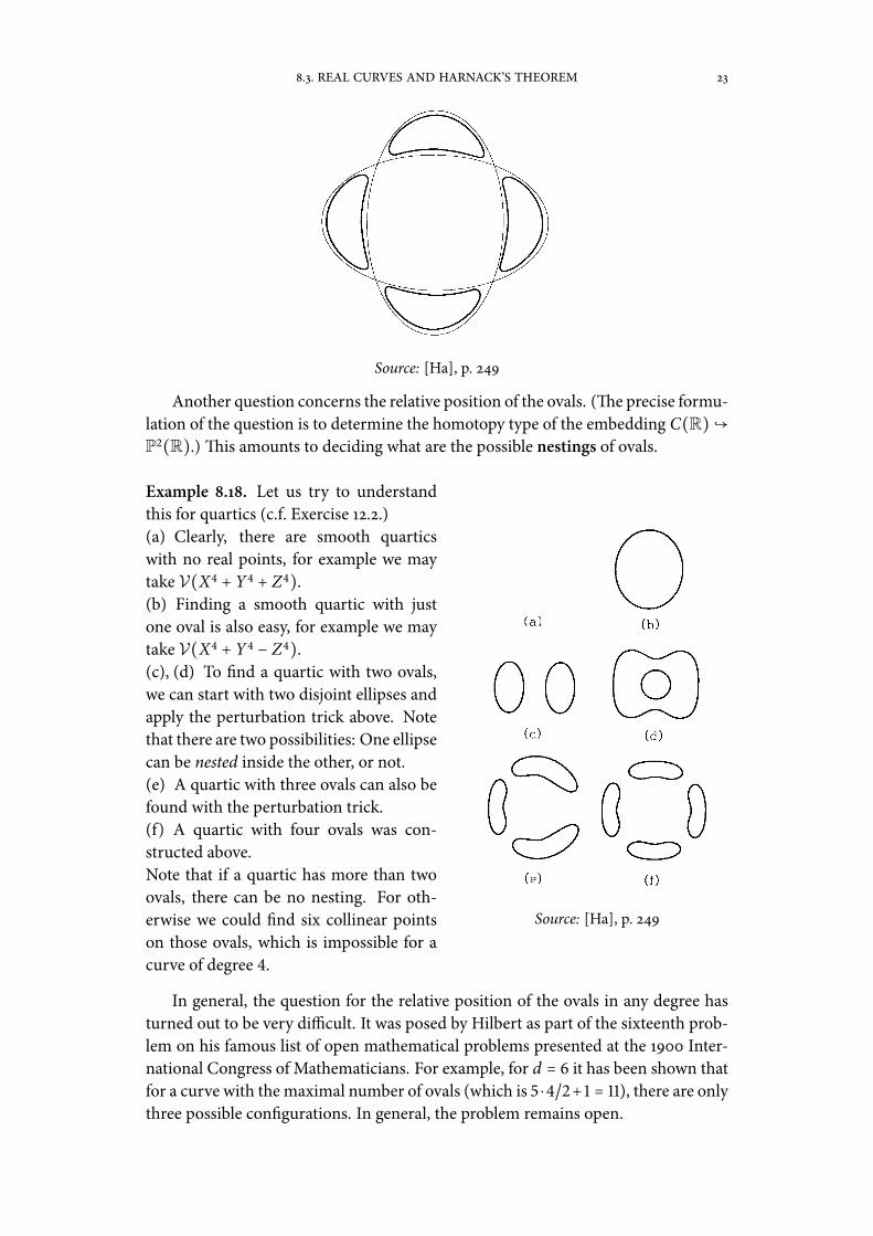
Another question concerns the relative position of the ovals. (�e precise formu-lation of the question is to determine the homotopy type of the embedding C(R)�P�(R).) �is amounts to deciding what are the possible nestings of ovals.

Example �.��. Let us try to understandthis for quartics (c.f. Exercise ��.�.)(a) Clearly, there are smooth quarticswith no real points, for example we maytake V(X� + Y� + Z�).(b) Finding a smooth quartic with justone oval is also easy, for example we maytake V(X� + Y� − Z�).(c), (d) To �nd a quartic with two ovals,we can start with two disjoint ellipses andapply the perturbation trick above. Notethat there are two possibilities: One ellipsecan be nested inside the other, or not.(e) A quartic with three ovals can also befound with the perturbation trick.(f) A quartic with four ovals was con-structed above.Note that if a quartic has more than twoovals, there can be no nesting. For oth-erwise we could �nd six collinear pointson those ovals, which is impossible for acurve of degree �.

Source: [Ha], p. ���

In general, the question for the relative position of the ovals in any degree hasturned out to be very di�cult. It was posed by Hilbert as part of the sixteenth prob-lem on his famous list of open mathematical problems presented at the ���� Inter-national Congress of Mathematicians. For example, for d = � it has been shown thatfor a curve with the maximal number of ovals (which is � ⋅���+ � = ��), there are onlythree possible con�gurations. In general, the problem remains open.