dependabilityzoomin.idt.mdh.se/course/kpp202/ht2010/le11asn101007/dependability_3.pdf ·...

COMPENDIUM: Dependability Copyright © Marcus Bengtsson and Antti Salonen, 2007 Rev: 2007-04-05 Report no. IDPIoDTR:07:02

1

Department of Innovation, Design and Product Development Marcus Bengtsson and Antti Salonen

Dependability –

Calculations in: Reliability,

Maintainability, Maintenance Supportability,

Availability, and Overall Equipment Effectiveness

Report no. IDPIoDTR:07:02


2

Contents 1. INTRODUCTION................................................................................... 3 2. RELIABILITY ........................................................................................ 4 2.1 CALCULATIONS ........................................................................................ 4 2.1.1 Reliability and Distribution function.................................................... 4 2.1.2 Failure rate, z(t) ................................................................................... 4 2.1.3 Reliability function, R(t) ....................................................................... 5 2.1.4 Mean Time To Failure, MTTF.............................................................. 5 2.1.5 Median time, tm..................................................................................... 5 2.1.6 Reliability block diagrams.................................................................... 6 3. MAINTAINABILITY............................................................................. 7 3.1 CALCULATIONS ........................................................................................ 7 3.1.1 Mean Time To Repair, MTTR............................................................... 7 3.1.2 Mean Maintenance Time, M(dash)....................................................... 8 3.1.3 Mean Time Between Maintenance, MTBM .......................................... 8 4. MAINTENANCE SUPPORTABILITY................................................ 9 4.1 CALCULATIONS ........................................................................................ 9 4.1.1 Waiting Times, MDT, MTW, MLDT..................................................... 9 5. AVAILABILITY ................................................................................... 12 5.1 CALCULATIONS ...................................................................................... 12 5.1.1 Availability, Ai, Aa, and Ao.................................................................. 12 6. OVERALL EQUIPMENT EFFECTIVENESS.................................. 13 6.1 Levels of OEE........................................................................................ 14 6.2 Mixed cycle times .................................................................................. 14 7. EXAMPLES........................................................................................... 15 8. REFERENCES ...................................................................................... 23


3

1. Introduction Within dependability one objective is to calculate different values within quality assurance. Dependability has been defined as (SS-EN 13306, 2001):

Collective term used to describe the availability and its influencing factors: reliability, maintainability, and maintenance supportability.

Dependability is thus used only for general descriptions in non-quantitative terms. The functions, though; reliability, maintainability, maintenance supportability, and the overall function, availability, can be described in quantitative terms. This compendiums objective is to describe how these can be calculated in an industrial setting. The compendium though will only focus on probabilities and likelihood approximations and will be delimited to the Exponential distribution only, see section 2.1.2 Failure rate for more information.

FIGURE 1 Overview of dependability with its influencing factors and in which chapter they will be discussed. The overall function, availability, has to do with an items ability to perform a required function under given conditions at a given instant of time or during a given time interval. Availability is usually measured in percentage (0-1) and is thus influenced by the other three factors according to fig. 1, namely: reliability, maintainability, and maintenance supportability. The reliability of an item has to do with its ability to function without appearances of faults or other disturbances. It thus has to do with the construction of a product or a system. The maintainability of an item has to do with how easy, fast, and resource parsimonious it is to repair and maintain the item, regarding both corrective and preventive maintenance. It is thus also a function that is closely tied to the construction of a product or a system. The maintenance supportability though has to do with the maintenance department of a company, i.e. number of employees, competence level, spare parts organization, tools, administration etc. and how this is all organized. In short, the reliability and maintainability of an item is closely related to the construction while the maintenance supportability is related to the organization, all need to strive for a good result in order to achieve a high availability.

Ch. 5 Availability

Ch. 2 Reliability Ch.3 Maintainability Ch. 4 Maintenance Supportability


4

2. Reliability TABLE 1 Concepts within reliability calculations. Concept Meaning Meaning (in Swedish) R(t) Reliability function Funktionssannolikhet F(t) Distribution function Fördelningsfunktion z(t) Failure rate Felbenägenhet f(t) Probability density Sannolikhetstäthet µ Mean Time To Failure Genomsnittlig tid till fel MTTF Mean Time To Failure Genomsnittlig tid till fel MTBF Mean Time Between Failure Genomsnittlig tid mellan fel tm Median time Mediantid (för beräkning av

medianlivslängder) CM Corrective maintenance Avhjälpande underhåll (AU) PM Preventive maintenance Förebyggande underhåll (FU) λ Failure rate (for exponential

distributions) Felintensitet (för exponentialfördelade tider till fel)

2.1 Calculations Calculations within reliability are a science in its own. Reliability has been defined as (SS-EN 13306, 2001):

Ability of an item to perform a required function under given conditions for a given time interval.

It thus has to do with failure and how often a failure occurs and what the implication of failure is. To calculate this with precise accuracy is of course very hard. We will therefore instead talk in terms of probability and likelihood approximations.

2.1.1 Reliability and Distribution function The reliability function, sometimes called survival function, is the quantitative value of the probability of function for an item at a specific time. The reliability function is denoted R(t), where t is the specific time one wants to calculate. As an example we can study R(1000) = 0.80, in where we find that 80% of all items in a specific lot survives 1000 time units. Unless else specified one time unit is equal to one hour. On a more negative note one can focus on the items that will not survive a specific time. This is denoted F(t), and is called distribution function. Let us study, F(1000) = 0.20, in where we find that 20% of all items in a specific lot will not survive 1000 hours. F(t) and R(t) is thus each others counterparts. In that we only can calculate with 100% (1.0) following Equation can be drawn:

)(1)( tFtR −= [1]

2.1.2 Failure rate, z(t) In order to calculate how often a failure occurs we use the term failure rate, z(t). The unit of failure rate is failure/time unit, i.e. failure/hour or h-1. Simplified, the failure rate can have


5

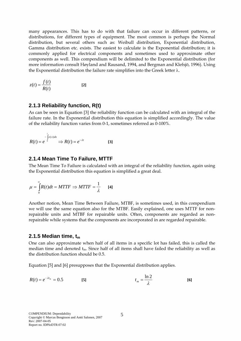
many appearances. This has to do with that failure can occur in different patterns, or distributions, for different types of equipment. The most common is perhaps the Normal distribution, but several others such as: Weibull distribution, Exponential distribution, Gamma distribution etc. exists. The easiest to calculate is the Exponential distribution; it is commonly applied for electrical components and sometimes used to approximate other components as well. This compendium will be delimited to the Exponential distribution (for more information consult Høyland and Rausand, 1994, and Bergman and Klefsjö, 1996). Using the Exponential distribution the failure rate simplifies into the Greek letter λ.

)()()(

tRtftz = [2]

2.1.3 Reliability function, R(t) As can be seen in Equation [3] the reliability function can be calculated with an integral of the failure rate. In the Exponential distribution this equation is simplified accordingly. The value of the reliability function varies from 0-1, sometimes referred as 0-100%.

tdxxz

etRetR

t

λ−−

=⇒∫

= )()( 0

)(

[3]

2.1.4 Mean Time To Failure, MTTF The Mean Time To Failure is calculated with an integral of the reliability function, again using the Exponential distribution this equation is simplified a great deal.

λµ 1)(

0

=⇒== ∫∞

MTTFMTTFdttR [4]

Another notion, Mean Time Between Failure, MTBF, is sometimes used, in this compendium we will use the same equation also for the MTBF. Easily explained, one uses MTTF for non-repairable units and MTBF for repairable units. Often, components are regarded as non-repairable while systems that the components are incorporated in are regarded repairable.

2.1.5 Median time, tm One can also approximate when half of all items in a specific lot has failed, this is called the median time and denoted tm. Since half of all items shall have failed the reliability as well as the distribution function should be 0.5. Equation [5] and [6] presupposes that the Exponential distribution applies.

5.0)( == − mtetR λ [5] λ

2ln=mt [6]


6

2.1.6 Reliability block diagrams Up till now we have only studied single components and how one can calculate different values. Naturally it is most common that components are connected with other components in a system to work toward the accomplishment of some purpose. The Equations below demonstrates how one can work with different constructions of systems, series and parallel and a mixture of these.

)(...)()()()( 211

tRtRtRtRtR n

n

jjs ⋅⋅⋅==∏

=

[7]

∏=

−⋅⋅−⋅−−=−−=n

jnjp tRtRtRtRtR

121 ))(1(...))(1())(1(1))(1(1)( [8]

Normally a system consists of a mixture of both series and parallel connections. To calculate such a system also the equations needs to be mixed, see below for example.

FIGURE 2 Examples of different systems. Example: In the figure above we can see three different systems but with similar components that has a reliability of R1(t) = 0.95 and R2(t) = 0.90. Calculate the reliability of the different systems. a) The system is a series system, we can therefore calculate the reliability as:

Rs(t) = 0.95 * 0.90 = 0.855 b) The system is a parallel system, we can therefore calculate the reliability as:

Rp(t) = 1-((1-0.95) * (1-0.90)) = 0.995 c) The system is a mixed system of both series and parallel, we can then mix the equations to

calculate the reliability of the system as: Rsystem(t) = 0.95 * (1-(1-0.95) * (1-0.90)) = 0.94525 Think through the different calculations, the results and answers, and why there is such a big difference. A team is only as strong as its weakest link is something people say in sports. How does that saying apply in this situation?

R1(t) R2(t)

R1(t)

R2(t)

R1(t)R2(t)

R1(t)

a) Series system

b) Parallel system c) Mixed system

A series system functions as long as all components in the system functions.

A parallel system functions as long as one component in the system functions.


7

3. Maintainability TABLE 2 Concepts within maintainability calculations. Concept Meaning Meaning (in Swedish) MTTR Mean Time To Repair Väntevärdet av den aktiva tiden för

AU med givna resurser MTBM Mean Time Between

Maintenance Genomsnittlig tid mellan UH-åtgärder (AU och/eller FU)

MTBMCM Mean Time Between Corrective Maintenance

Genomsnittlig tid mellan avhjälpande UH-åtgärder

MTBMPM Meat Time Between Preventive Maintenance

Genomsnittlig tid mellan förebyggande UH-åtgärder

__

M sometimes written as M(dash)

Mean Maintenance Time Väntevärdet av den aktiva tiden för UH med givna resurser

CMM__

(=MTTR) Mean active corrective maintenance time

Väntevärdet av den aktiva tiden för AU med givna resurser

PMM__

Mean active preventive maintenance time

Väntevärdet av den aktiva tiden för FU med givna resurser

f Frequency of preventive maintenance tasks

Frekvens av förebyggande underhållsåtgärder

λ Failure rate (for exponential distributions)

Felintensitet (för exponentialfördelade tider till fel)

3.1 Calculations Maintainability has been defined as (SS-EN 13306, 2001):

Ability of an item under given conditions of use, to be retained in, or restored to, a state in which it can perform a required function, when maintenance is performed under given conditions and using stated procedures and resources.

Maintainability is thus values on how easy as well as how fast and resource parsimonious it is to correct a possible disturbance or failure. Maintainability calculations takes in both corrective and preventive maintenance, but one is also able to keep them apart for possibilities to calculate different availabilities.

3.1.1 Mean Time To Repair, MTTR Mean Time To Repair, MTTR, is the actual time it takes to perform corrective maintenance. It is thus a maintenance activity that takes place after a function failure has been discovered. The time unit is usually, if not prescribed other, in hours.

CM

ii

iii MM

MTTR__

=Σ

⋅Σ=

λ

λ [9]

Mi is the repair time for fault type i and λi is the failure rate for fault type i. We can, with data for these figures, calculate the MTTR or Mean active corrective maintenance time.


8

3.1.2 Mean Maintenance Time, M(dash) To be able to calculate the Mean Maintenance Time all in all, that is to say the total time of maintenance considering both corrective and preventive maintenance tasks we first need to calculate the Mean active preventive maintenance time.

jj

jjjPM

f

MfM

Σ

⋅Σ=

__

[10]

Mj is the maintenance time for preventive maintenance activity j and fj is the frequency of preventive maintenance for maintenance activity j.

fMfMM PMCM

+⋅+⋅

=λ

λ____

__

[11]

All in all we can calculate the Mean Maintenance Time considering both corrective and preventive maintenance.

3.1.3 Mean Time Between Maintenance, MTBM To calculate the Mean Time Between Maintenance, MTBM, we need the values on MTBMCM and MTBMPM or the failure rate and frequency of preventive maintenance as λ = 1/MTTF, λ = 1/MTBF, or λ = 1/MTBMCM and f = 1/MTBMPM.

PMCM MTBMMTBMMTBM

111+

= [12]


9

4. Maintenance Supportability TABLE 3 Concepts within maintenance supportability calculations. Concepts Meaning Meaning (in Swedish) MDT Mean Down Time Genomsnittlig funktionsavbrottstid MTW Mean Time Waiting Genomsnittlig väntetid MTW(A) Mean Time Waiting

Administrative Administrativ väntetid

MTW(A)CM Mean Time Waiting Administrative for corrective maintenance

Administrativ väntetid vid AU

MTW(A)PM Mean Time Waiting Administrative for preventive maintenance

Administrativ väntetid vid FU

MLDT Mean Logistic Down Time Genomsnittlig tid för väntan (transporter) på UH-resurser

MLDTCM Mean Logistic Down Time for corrective maintenance

Genomsnittlig tid för väntan (transporter) på AU-resurser

MLDTPM Mean Logistic Down Time for preventive maintenance

Genomsnittlig tid för väntan (transporter) på FU-resurser

4.1 Calculations Maintenance supportability has been defined as (SS-EN 13306, 2001):

Ability of a maintenance organization of having the right maintenance support at the necessary place to perform the required maintenance activity at a given instant of time or during a given time interval.

Maintenance supportability is thus values on how well a maintenance organization is functioning considering staff, tools, administrative functions etc. In a realistic setting it of course takes more time to correct a failure than the actual time it takes to perform the actual maintenance activity. Sometimes spare parts has to be ordered, sometimes it takes special competence to repair a fault that might not exist within the ordinary staff, sometimes special tools needs to be purchased, sometimes a maintenance activity might need some administrative work before it can be executed etc.

4.1.1 Waiting Times, MDT, MTW, MLDT The Equations below shows how one can work with waiting times, taking in waiting times such as logistics, administrative, and the actual maintenance time. There is not really any set standards as to what times should be associated with logistic or administrative waiting times, this is something every company needs to decide about. In order to calculate the waiting times it is as it is to calculate the Mean Maintenance Time wise to keep the waiting time for corrective and preventive maintenance apart, this in order to see where progress and efficiency measure can be performed. MLDT is an abbreviation of Mean Logistics Down Time, MTW(A) is Mean Time Waiting Administrative, MTW is Mean Time Waiting and MDT is Mean Down Time.


10

∑∑ ⋅

=

ii

iii

CM

MLDTMLDT

λ

λ [13]

MLDTi is the Mean Logistics Down Time for corrective maintenance activity i and λi is the failure rate for fault type i.

∑∑ ⋅

=

jj

jjj

PM f

MLDTfMLDT [14]

MLDTj is the Mean Logistics Down Time for preventive maintenance activity j and fj is the frequency of preventive maintenance for maintenance activity j.

fMLDTfMLDTMLDT PMCM

+⋅+⋅

=λ

λ [15]

All in all, we can calculate the Mean Logistics Down Time considering both corrective and preventive maintenance.

∑∑ ⋅

=

ii

iii

CM

AMTWAMTW

λ

λ )()( [16]

MTW(A)i is the Mean Time Waiting Administrative for corrective maintenance activity i and λi is the failure rate for fault type i.

∑∑ ⋅

=

jj

jjj

PM f

AMTWfAMTW

)()( [17]

MTW(A)j is the Mean Time Waiting Administrative for preventive maintenance activity j and fj is the frequency of preventive maintenance for maintenance activity j.

fAMTWfAMTWAMTW PMCM

+⋅+⋅

=λ

λ )()()( [18]

All in all we can calculate the Mean Time Waiting Administrative considering both corrective and preventive maintenance.


11

)(AMTWMLDTMTW += [19]

The Mean Time Waiting can then be calculated according Equation [19].

__MMTWMDT += [20]

The Mean Down Time can then be calculated according Equation [20].

fMMLDTAMTWfMMLDTAMTW

MDT PMPMPMCMCMCM

+++⋅+++⋅

=λ

λ ))(())((____

[21]

All in all, for visual effect, we can calculate the Mean Down Time according Equation [21].


12

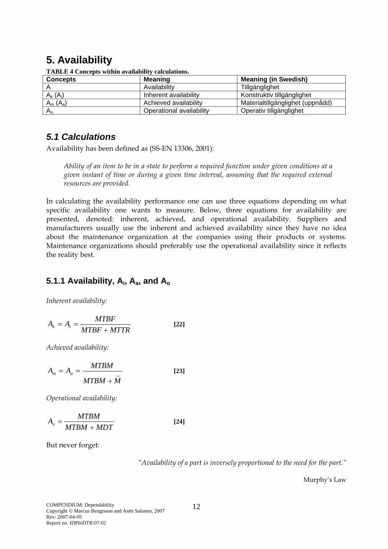
5. Availability TABLE 4 Concepts within availability calculations. Concepts Meaning Meaning (in Swedish) A Availability Tillgänglighet Ak (Ai) Inherent availability Konstruktiv tillgänglighet Am (Aa) Achieved availability Materialtillgänglighet (uppnådd) Ao Operational availability Operativ tillgänglighet

5.1 Calculations Availability has been defined as (SS-EN 13306, 2001):

Ability of an item to be in a state to perform a required function under given conditions at a given instant of time or during a given time interval, assuming that the required external resources are provided.

In calculating the availability performance one can use three equations depending on what specific availability one wants to measure. Below, three equations for availability are presented, denoted: inherent, achieved, and operational availability. Suppliers and manufacturers usually use the inherent and achieved availability since they have no idea about the maintenance organization at the companies using their products or systems. Maintenance organizations should preferably use the operational availability since it reflects the reality best.

5.1.1 Availability, Ai, Aa, and Ao Inherent availability:

MTTRMTBFMTBFAA ik +

== [22]

Achieved availability:

__MMTBM

MTBMAA am

+== [23]

Operational availability:

MDTMTBMMTBMAo +

= [24]

But never forget:

“Availability of a part is inversely proportional to the need for the part.”

Murphy’s Law


13

6. Overall Equipment Effectiveness In order to measure the effectiveness of production equipment and also to back track the lack of effectiveness to its sources, OEE is often used. OEE is a loosely defined measurement more focusing on usability than accuracy. The original definition was made by Nakajima (1989) who means that OEE is a very useful indicator for the performance of a production facility. Nakajima (1989) defines OEE as stated below: OEE = Availability x Performance rate x Quality rate

Availability measures the amount of production time that is lost due to failures, change over, adjustments, and other types of down time (Bamber, et al., 2003). The measurement is the quota between actual operative time and planned, available operative time. This definition is based on planned available production time which is not the same as theoretically available production time. This fact, mean Bamber et al. (2003), is a problem since for example planned maintenance is not considered a loss. This fact means that there is no incitement for rationalization of the preventive maintenance. Ljungberg (1998) means that the availability should be calculated based on full calendar time i.e. 8760 hours available production time per year. Ljungberg (1998) as well as Jeong and Phillips (2001) argue that Nakajima’s definition of OEE does not consider planned stops as much as would be desired. Performance rate is the quota between real performance and theoretical performance. Nakajima uses a time based measurement while De Groote (1995) for example uses the quota between achieved production volume and theoretical production volume. The two different bases for calculation, however, give the same result (Bamber et al., 2003). Quality rate is the quota between number of defect free products and number of produced products. Bamber et al. (2003) point out that this calculation is based on defects detected in direct proximity to the measured operation. A wider definition of quality rate would, as Bamber et al. (2003) see it, be desired, but it would probably become more complicated to use.

Availability = Planned production time – stop time Planned production time

Performance rate = Bought cycle time x items produced Available operative time

Quality rate = Items produced – defect items

Items produced


14

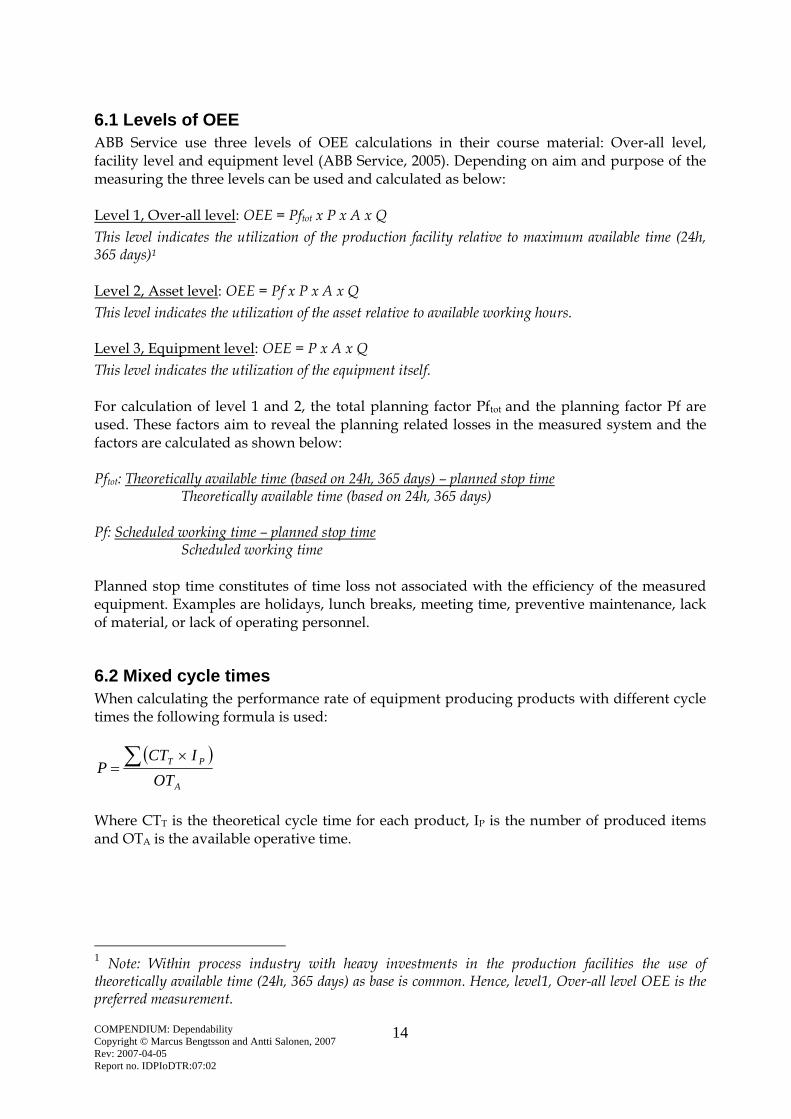
6.1 Levels of OEE ABB Service use three levels of OEE calculations in their course material: Over-all level, facility level and equipment level (ABB Service, 2005). Depending on aim and purpose of the measuring the three levels can be used and calculated as below: Level 1, Over-all level: OEE = Pftot x P x A x Q This level indicates the utilization of the production facility relative to maximum available time (24h, 365 days)1 Level 2, Asset level: OEE = Pf x P x A x Q This level indicates the utilization of the asset relative to available working hours. Level 3, Equipment level: OEE = P x A x Q This level indicates the utilization of the equipment itself. For calculation of level 1 and 2, the total planning factor Pftot and the planning factor Pf are used. These factors aim to reveal the planning related losses in the measured system and the factors are calculated as shown below: Pftot: Theoretically available time (based on 24h, 365 days) – planned stop time Theoretically available time (based on 24h, 365 days) Pf: Scheduled working time – planned stop time Scheduled working time Planned stop time constitutes of time loss not associated with the efficiency of the measured equipment. Examples are holidays, lunch breaks, meeting time, preventive maintenance, lack of material, or lack of operating personnel.

6.2 Mixed cycle times When calculating the performance rate of equipment producing products with different cycle times the following formula is used:

( )A

PT

OTICT

P ∑ ×=

Where CTT is the theoretical cycle time for each product, IP is the number of produced items and OTA is the available operative time.

1 Note: Within process industry with heavy investments in the production facilities the use of theoretically available time (24h, 365 days) as base is common. Hence, level1, Over-all level OEE is the preferred measurement.


15

7. Examples Example 1 A machine has a value of MTTR of 1 hour; the machine fails its operation every 300 hour. Calculate the machines’ inherent availability. Example 2 A machine has an inherent availability of 0.99. The machine fails its operation every 400 hour. Calculate the machines’ MTTR. Example 3 Consider a machine with exponentially distributed time to failure with following data: Failure rate, λ = 0.0015 faults/hour MTTR = 3h MTBMPM = 3000h M(dash)PM = 3h Calculate the achieved availability. Example 4 A machine have a MTBF of about 1000h, the same machine has a preventive maintenance schedule saying it needs maintenance every 200 hour. Calculate the Mean Time Between Maintenance, MTBM. Example 5 Consider a machine with exponentially distributed time to failure with following data: λ = 0.001 faults/h f = 0.0001 times/h M(dash)CM = 1h M(dash)PM = 3h Calculate Mean Time Between Maintenance, MTBM and the Mean Maintenance Time M(dash). Example 6 Consider a machine with exponentially distributed time to failure with following data: MTBM = 750h MLDT = 8h MTW(A) = 4h M(dash) = 1h Calculate the operational availability. Suggest how the company might be able to increase the operational availability and calculate again.


16

Example 7 Consider a machine with exponentially distributed time to failure with following data: λ = 0.004 faults/h f = 0.002 times/h M(dash)CM = 3h M(dash)PM = 2h Calculate the inherent and the achieved availability. Example 8 Consider a machine with exponentially distributed time to failure with failure rate λ = 200x10-

6 fault/h and a Mean Down Time of 40 hours, calculate the operative availability. Example 9 A laser machine that is run in dayshift, 8h/day, 200 days/year, are usually maintained 15 times/year. A repairman is leased from another company every time the machine fails to operate. It takes the repairman about 1.5 hours of travel to make it to the laser machine and roughly 5 hours to repair it. The paperwork takes about 1 hour of the previously mentioned 5. Of all the maintenance occasions, 10 are caused by unexpected breakdowns, the rest of the occasions are preventive maintenance that takes about 8 hours every time. Calculate the inherent, achieved, and operational availability of the laser machine. Example 10 A machine has a measured value of the achieved availability of 0.8. The Mean Time Between Maintenance is 100 hours, the Mean Time To Repair is 36 hours, the Mean Time Between Failure is 200h, and M(dash) PM is 2 hours. Calculate with what frequency that preventive maintenance was carried out on this specific machine. (The example contains a built in fault, there is a possibility to calculate the frequency in two different approaches which will give two different answers.) Example 11 Consider a machine with exponentially distributed time to failure with following data: MTBF = 110 h MTBM = 55 h M(dash) = 1.5 h MTW(A) = 1 h MTTR = 2.5 h MLDT = 1 h Calculate the inherent, achieved, and operational availability.


17

Example 12 Consider a machine with exponentially distributed time to failure with following data: MTBF = 1000 h MTTR = 4 h M(dash)PM = 1.5 h MTBMPM = 200 h MTW(A) = 1 h MLDT = 0.5 h Calculate the inherent, achieved, and operational availability. Example 13 Consider a machine with exponentially distributed time to failure with following data: MTBM = 1000 h M(dash) = 1.2 h Ao = 0.96 Calculate the Mean Time Waiting. Example 14 A system has a Mean Time Between Failure of 500 hours and a Mean Time To Repair of 5 hours. The system is run continuously around the clock with a production value of 15 000 SEK/hour. Calculate if a modification of the system so that the MTTR would decrease to 4 hours with a once-for-all payment of 150 000 SEK prove to be a wise investment seen out of perspective of the inherent availability. Example 15 A system has an achieved availability of 0.985 and a Mean Time Between Maintenance of 300 hours, calculate the Mean Maintenance Time. Example 16 Consider a machine with exponentially distributed time to failure with following data: λ = 0.001 faults/h MTTR = 1.5 h MTBMPM = 2500 h M(dash)PM = 1 h MTW(A)CM = 1.2 h MTW(A)PM = 0.2 h MLDTCM = 1.5 h MLDTPM = 0 h Calculate the inherent, achieved, and operational availability.


18

Example 17 A manufacturing company is experiences problems with a low availability on one of their production systems. The equipment works according the figure below.

It is the station 3 that does not work satisfactorily. The other equipment all together has an availability of 85%. Following data has been measured for station 3, failure occurs in mean every 5 hours and it takes approximately 1.5 hours to repair these. The company wishes to increase the availability on station 3 so that all equipment together receives an availability of 80%. What must the company decrease the Mean Time To Repair to, alternatively, what must they increase the Mean Time Between Failures to in order to achieve the goal. Example 18 An indicator, measuring oil level, need a reliability of Rsystem = 0.95. The system comprises of four components in series with the following reliability: Sensor R1 = 0,985 Indicator R2 =0,985 Instrument R3 =0,990 Relay R4 = unknown What reliability is required on the relay? Example 19 Calculate the reliability of an electric system with 25 mass produced components where each component has the reliability 0.985. The system is connected in series. Calculate again but consider the system being connected in parallel. Example 20 Calculate the median time for a component that has Exponential distributed time to failure with the failure rate λ. Example 21 Consider two components with Exponential distributed time to failure with the parameters λ1 and λ2, calculate the Mean Time Between Failure for a system with these components if they are connected in:

a) Series b) Parallel

Station 1 Conveyer belt Station 2 Station 3


19

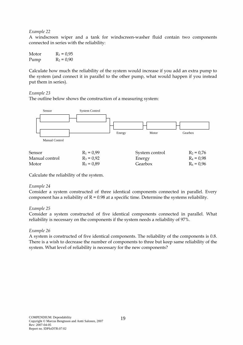
Example 22 A windscreen wiper and a tank for windscreen-washer fluid contain two components connected in series with the reliability: Motor R1 = 0,95 Pump R2 = 0,90 Calculate how much the reliability of the system would increase if you add an extra pump to the system (and connect it in parallel to the other pump, what would happen if you instead put them in series). Example 23 The outline below shows the construction of a measuring system:

Sensor R1 = 0,99 System control R2 = 0,76 Manual control R3 = 0,92 Energy R4 = 0,98 Motor R5 = 0,89 Gearbox R6 = 0,96 Calculate the reliability of the system. Example 24 Consider a system constructed of three identical components connected in parallel. Every component has a reliability of R = 0.98 at a specific time. Determine the systems reliability. Example 25 Consider a system constructed of five identical components connected in parallel. What reliability is necessary on the components if the system needs a reliability of 97%. Example 26 A system is constructed of five identical components. The reliability of the components is 0.8. There is a wish to decrease the number of components to three but keep same reliability of the system. What level of reliability is necessary for the new components?

Manual Control

Sensor System Control

Energy Motor Gearbox


20

Example 27

Consider a machine with exponentially distributed time to failure with following data: λ1 = 0.001 fault/h λ2 = 0.0025 fault/h Calculate the reliability after 100 hours. Example 28 Consider a machine with exponentially distributed time to failure with following data: λ = 0.0001 fault/h Calculate the MTTF, median time, and reliability after 1000, 10 000, and 100 000 hours. Example 29

R1 = 0.99 R2 = 0.99 R3 = 0.995 R4 = 0.985 Rsystem = ? Calculate Rsystem. Example 30 Consider an electronic component with Exponential distributed time to failure with the failure rate λ = 0.001 faults/hour. If you want to exchange the component when the reliability has decreased to 0.95, how many hours can you let it run?

λ1

λ2

λ2

R1 R2

R3

R3

R1

R2

R3

R4


21

Example 31 A system consists of three components connected in parallel with the failure rate 0.001. What is the reliability after 1000 hours for the system as well as the components? Example 32 Calculate the Asset effectiveness PfOEE and Equipment effectiveness OEE for a milling machine under the following circumstances: Production time: 2-shift, Mon.-Fri.

Shift hours: Morning shift, 06:00 – 14:12 Afternoon shift, 13:48 – 22:00, fridays, 13:48 - 20:00

Lunch break: 30 minutes lunch each shift, with no production.

Meetings: Department meeting every Thursday, 12:48 – 13:48, without production.

Maintenance: Preventive maintenance is performed daily, 13:48 – 14:00.

Production speed: The equipment has a bought cycle time of 6 minutes per product.

Outcome during one week

Break downs: Mon. 08:30 – 10:00 Wed. 07:00 – 10:12 Thu. 15:30 – 17:24

Actual production: 523 items of which 3 items were scrap.


22

Answers: 1. Ai = 0.9967 2. MTTR = 4.04h 3. Aa = 0.9945 (MTBM = 545.45h and M(dash) = 3h) 4. MTBM = 166.7h 5. MTBM = 909.1h, M(dash) = 1.182h 6. Ao = 0.983, both MLDT and MTW(A) feels unnecessarily high, if decreasing these to half (through better planning, spare part planning, contract with suppliers etc.) the operational availability increases to 0.991. 7. Ai = 0.988 and Aa = 0.984 8. Ao = 0.992 9. Ak = 0.976, Aa = 0.952 samt Ao = 0.944 10. f = 2.39x10-3

11. Ai = 0.977, Aa = 0.973 and Ao = 0.940 12. Ai = 0.9960, Aa = 0.9886 and Ao = 0.9799 13. MTW = 40,467 h 14. Yes, if calculated in one year. Aold = 0.990, equals 87.6 hours in production losses (cost for this 1 314 000 SEK). Anew = 0.992, equals 70.08 hours in production losses (cost for this 1 051 200 SEK). 15. M(dash) = 4.568 h 16. Ai = 0.9985, Aa = 0.9981 and Ao = 0.9953 17. MTTR = 0.3125h = 18.75 min, MTBF = 23.92 h 18. R4 > 0.989 19. RS = 0.685, RP = 1 20. tm = (ln2)/λ 21. MTBFS = 1/(λ1 + λ2), MTTFP = 1/λ1 + 1/λ2 - 1/(λ1 + λ2) 22. From R = 0.855 to R = 0.9405 23. RSystem = 0.82 24. R System = 0.999 25. R Component = 0.504 26. The new components need R = 0.9316 27. R(100) = 0.8605 28. MTTF = 10000 h, tm = 6931 h, R(1000) = 0.905, R(10000) = 0.368, R(100000) = 0.000045 29. Rsystem = 0.965 30. t = 51.3 h 31. RComponent(1000) = 0.3678, Rsystem(1000) = 0.747 32. PfOEE = 66.6%, OEE = 73.2%


23

8. References ABB Service, (2005). Powerpoint presentation: “TAK-definitioner 051117”. Bamber, C.J. Castca, P. Sharp, J.M. and Motara, Y., (2003). Cross-functional team working for overall equipment effectiveness (OEE), Journal of Quality in Maintenance Engineering, Vol. 9 No. 3, pp. 223-238. Bergman, B. och Klefsjö, B. (1996). Tillförlitlighet. Studentlitteratur, Luleå Tekniska Universitet. Bergman, B. och Klefsjö, B. (2001). Kvalitet – från behov till användning. Studentlitteratur, Lund. Blomgren, S. (1993). Underhållsmässighet. Faktarapport, Sveriges Verkstadsindustrier, Industrilitteratur. De Groote, P. (1995). Maintenance performance analysis: a practical approach, Journal of Quality in Maintenance Engineering, Vol. 1 No. 2, pp. 4-24. Høyland, A. and Rausand, M. (1994). System Reliability Theory – Models and Statistical Methods. USA: John Wiley & Sons, Inc. Jeong, K. Phillips, D. T. (2001). Operational efficiency and effectiveness measurement, International Journal of Operations and Production Management, Vol. 21 No. 11, pp. 1404-1416. Johansson, K-E. (1993). Driftsäkerhet och underhåll. Studentlitteratur, Lund. ISBN 91-44-39111-0. Ljungberg, Ö. (1998). Measurement of overall equipment effectiveness as a basis for TPM activities, International Journal of Operations & Production Management, Vol. 18 No. 5 pp. 495-507. Nakajima, S. (1989). TPM Development Program. Cambridge: Productivity Press Inc. Stenmark, J. (1996). Underhållssäkerhet. Faktarapport, Sveriges Verkstadsindustrier, Industrilitteratur. Svensk Standard SS-EN 13306. (2001). Underhåll – Terminologi. SIS, Swedish Standards Institute.

dependabilityzoomin.idt.mdh.se/course/kpp202/ht2010/le11asn101007/dependability_3.pdf ·...

Documents