€¦ · dr. eugene terray woods hole oceanographic institution – technical lead dr. brian howes,...

OCS Study BOEM 2014-604

US Department of the Interior Bureau of Ocean Energy Management Office of Renewable Energy Programs

Roadmap: Technologies for Cost Effective, Spatial Resource Assessments for Offshore Renewable Energy

US Department of the Interior Bureau of Ocean Energy Management Office of Renewable Energy Programs January, 2014

Roadmap: Technologies for Cost Effective, Spatial Resource Assessments for Offshore Renewable Energy

Authors

Dr. Eugene Terray Woods Hole Oceanographic Institution – Technical Lead Dr. Brian Howes, University of Massachusetts Dartmouth Mr. William Stein, University of Massachusetts Amherst Dr. Jon McGowan, University of Massachusetts Amherst Dr. James Manwell, University of Massachusetts Amherst Dr. Pierre Flament, University of Hawaii Dr. William Plant, University of Washington Dr. Paul Dragos, Battelle Memorial Institute Dr. Dennis Triza, Imaging Science Research Mr. Robert Anderson, Ocean Server Technology Dr. Jerry Mullison, Teledyne RD Instruments Prepared under BOEM Contract M10PC00096 by University of Massachusetts-Dartmouth Marine Renewable Energy Center (MREC) 151 Martine St., Fall River, MA 02723

i

DISCLAIMER This study was administered by the US Department of the Interior, Bureau of Ocean Energy Management, Environmental Studies Program, Washington, DC. Funding for the study was provided through the National Oceanographic Partnership Program (NOPP) project # M10PS00152 FY10. Additional partial funding for this study came from the US Department of Energy and National Oceanic and Atmospheric Administration. This report has been technically reviewed by BOEM and it has been approved for publication. The views and conclusions contained in this document are those of the authors and should not be interpreted as representing the opinions or policies of the US Government, nor does mention of trade names or commercial products constitute endorsement or recommendation for use.

REPORT AVAILABILITY To download a PDF file of this Environmental Studies Program report, go to the US Department of the Interior, Bureau of Ocean Energy Management, Environmental Studies Program Information System website and search on OCS Study BOEM 2014-604. This report can be viewed at select Federal Depository Libraries. It can also be obtained from the National Technical Information Service; the contact information is below.

US Department of Commerce National Technical Information Service 5301 Shawnee Rd. Springfield, VA 22312 Phone: (703) 605-6000, 1(800)553-6847 Fax: (703) 605-6900 Website: http://www.ntis.gov/

CITATION Terray, E., B. Howes, W. Stein, J. McGowan, J. Manwell, P. Flament, W. Plant, P. Dragos, D.

Triza, R. Anderson, and J. Mullison. 2014. Roadmap: Technologies for Cost Effective, Spatial Resource Assessments for Offshore Renewable Energy. US Dept. of the Interior, Bureau of Ocean Energy Management, Office of Renewable Energy Programs, Herndon. OCS Study BOEM 2014-604. 169 pp.

ABOUT THE COVER Front cover photo: Boston Light located on Little Brewster Island about 2.5 miles off Hull, MA. Electric power is available and it is an excellent site for wind resource assessment data gathering. Photo provided by UMass Amherst.

http://www.boem.gov/Environmental-Stewardship/Environmental-Studies-Program-Information-System.aspx

http://www.boem.gov/Environmental-Stewardship/Environmental-Studies-Program-Information-System.aspx

http://www.ntis.gov/

ii

TABLE OF CONTENTS 1 EXECUTIVE SUMMARY ......................................................................................... 1 2 RESEARCH SYNOPSIS .......................................................................................... 5

2.1 Introduction ........................................................................................................ 5 2.2 Focus and Aims of Individual Research Programs ............................................. 6 2.3 Summary of Individual Research Programs ....................................................... 7

2.3.1 High Resolution Wind Observations ............................................................ 7 2.3.2 Statistical Characterization of Winds, Waves and Currents over Larger Areas 10 2.3.3 High Resolution, Spatial Imaging of Waves and Currents ......................... 11 2.3.4 High Resolution Profiling of Currents and Turbulences ............................. 13 2.3.5 Spatial Surveys of Bottom Sediment and Biotic Communities ................... 14

3 HIGH RESOLUTION WIND PROFILING FROM BUOYS AND SMALL BOATS .... 16

3.1 Technical summary .......................................................................................... 16 3.2 Introduction/Background .................................................................................. 17

3.2.1 Overview .................................................................................................... 17 3.2.2 Potential Wind Measurement Systems ...................................................... 18 3.2.3 SODAR and LIDAR systems ..................................................................... 18 3.2.4 Other potential remote sensing systems.................................................... 18

3.3 Scope of Report ............................................................................................... 19 3.4 Review of State-of-the-art Instrumentation for SODAR and LIDAR ................. 19

3.4.1 SODAR: Principles of Operation ................................................................ 19 3.4.2 Wind Energy SODAR Applications ............................................................ 21 3.4.3 LIDAR Principles of Operation ................................................................... 24 3.4.4 Offshore Wind Energy LIDAR Applications................................................ 27 3.4.5 Summary of Current Manufacturers and Specifications............................. 33

3.5 Potential Sea Platforms for Instrumentation ..................................................... 38 3.5.1 Fixed Platforms .......................................................................................... 38 3.5.2 Long Term Platforms ................................................................................. 38 3.5.3 Short Term Platforms................................................................................. 39 3.5.4 Nearby Islands ........................................................................................... 40 3.5.5 Re-tasking an Existing Offshore Structure ................................................. 42 3.5.6 Coastal Onshore Location ......................................................................... 43 3.5.7 Floating Platforms ...................................................................................... 43 3.5.8 SeaZephIR ................................................................................................ 44 3.5.9 AXYS WindSentinel ................................................................................... 45 3.5.10 FLiDAR ...................................................................................................... 45 3.5.11 Fugro Seawatch ........................................................................................ 46

3.6 Recommendations/Conclusions ....................................................................... 47 3.7 References ....................................................................................................... 49

4 COHERENT MARINE AND HF RADAR VALIDATION TESTS FOR MEASUREMENT OF OCEAN WAVES AND CURRENT .............................................. 56

iii

4.1 Coherent Marine Radar Measurements of Directional Wave Spectra Using Vertically Polarized Antennas .................................................................................... 56

4.1.1 Technical summary ................................................................................... 56 4.1.2 OMEGA-K Spectra .................................................................................... 56 4.1.3 Coherent Radar Description ...................................................................... 57 4.1.4 OMEGA-K Spectra of CORrad .................................................................. 60 4.1.5 Frequency Spectra and Hm0 ..................................................................... 61 4.1.6 H-Polarization: Hurricane Ida ..................................................................... 62 4.1.7 V-Polarization: Hurricane Irene .................................................................. 63 4.1.8 Summary ................................................................................................... 64

4.2 DEVELOPMENT AND VALIDATION OF NEW COMPACT HF RADAR .......... 65 4.2.1 Technical Summary ................................................................................... 65 4.2.2 Introduction ................................................................................................ 66 4.2.3 New Hardware Developments ................................................................... 66 4.2.4 Sea Scatter Doppler Spectra ..................................................................... 68 4.2.5 2nd Order Doppler Continuum Due to Longer Wave Spectrum Components .......................................................................................... 70 4.2.6 Inversion of the Doppler Spectrum for Ocean Wave Spectra .................... 72 4.2.7 Acknowledgements ................................................................................... 72 4.2.8 References ................................................................................................ 72

5 HIGH RESOLUTION, SPATIAL IMAGING OF WINDS, CURRENTS AND BATHYMETRY .............................................................................................................. 74

5.1 Technical Summary ......................................................................................... 74 5.2 Introduction ...................................................................................................... 74 5.3 The Coherent Real Aperture Radar (CORAR) ................................................. 76 5.4 The R/V Thompson Cruise ............................................................................... 78 5.5 Wind Measurements ........................................................................................ 80 5.6 Current and Doppler Measurements ................................................................ 83 5.7 Wave Measurements, Phase-resolved and Statistical ..................................... 86 5.8 Conclusions...................................................................................................... 97 5.9 References ....................................................................................................... 99

6 MAPPING CURRENTS AND WAVES USING DOPPLER SONAR ..................... 102

6.1 Technical Summary ....................................................................................... 102 6.2 Turbulence Measurement Approaches .......................................................... 102 6.3 Mixed Sea State ............................................................................................. 102 6.4 Groups ........................................................................................................... 103 6.5 Background .................................................................................................... 103

6.5.1 Spatial Domain Processing for Horizontal ADCP Waves......................... 105 6.5.2 Traditional Time Domain Horizontal ADCP Deployment ......................... 105

6.6 Deployment Details ........................................................................................ 105 6.7 Raw Data ....................................................................................................... 106

6.7.1 Spatial Domain Results ........................................................................... 108 6.7.2 A Simple Approach for Estimating Wave Direction .................................. 110 6.7.3 Steps Investigated ................................................................................... 111

iv

6.7.4 The Value of Knowing Wave Direction .................................................... 113 6.8 Looking for Frequency/Phase Rate of Change .............................................. 113 6.9 Looking for Approaching Waves in Time ........................................................ 115 6.10 Turbulence ..................................................................................................... 116

6.10.1 Outer Scale Turbulence ........................................................................... 117 6.10.2 Turbulence Measurement Through Subscale Decorrelation.................... 119 6.10.3 Turbulent Spectra .................................................................................... 120

7 SURVEYS OF BOTTOM SEDIMENT AND BIOTIC COMMUNITIES .................. 121

7.1 Technical Summary ....................................................................................... 121 7.2 Background .................................................................................................... 122 7.3 Navigational Precision .................................................................................... 124 7.4 Acoustic Doppler Current Profiling ................................................................. 128 7.5 Side Scan Sonar ............................................................................................ 133 7.6 Multi-beam Sonar ........................................................................................... 139 7.7 Sediment Photography ................................................................................... 142 7.8 Sub-bottom Profiling ....................................................................................... 147 7.9 Conclusions.................................................................................................... 147

8 GEO-REFERENCING AND DATA MANAGEMENT ............................................ 148

8.1 Technical Summary ....................................................................................... 148 9 CONCLUSIONS ................................................................................................... 149

v

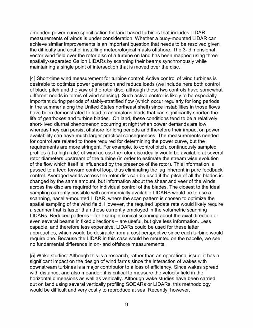
LIST OF FIGURES Figure 3-1: Measurement Solutions of Offshore Wind Projects .................................... 17 Figure 3-2: An Autonomous SUMO airplane and Ground Control Station. . ................ 19 Figure 3-3: The MVCO Platform (UMass photo) ........................................................ 22 Figure 3-4: Time Series of UMass MVCO SODAR Data .............................................. 23 Figure 3-5: Beam path in typical LIDAR ....................................................................... 25 Figure 3-6: Basic Components of a LIDAR System ..................................................... 26 Figure 3-7: Schematic of Risø Multi-Lidar System. ...................................................... 30 Figure 3-8: LIDAR at FINO 1 Offshore Platform ........................................................... 32 Figure 3-9: Left- Natural Power LIDAR System; Right- Leosphere WINDCUBE

LIDAR System. ........................................................................................................ 33 Figure 3-10: Sgurr (left) and Catch the Wind/Vindicator (BlueScout) LIDAR Systems

(right). ...................................................................................................................... 34 Figure 3-11: Lockheed Martin LIDAR System. ............................................................. 34 Figure 3-12: Cape Wind meteorological tower and Naikun Platform. ........................... 39 Figure 3-13: Jack-up Barge .......................................................................................... 40 Figure 3-14: Little Brewster Island ................................................................................ 41 Figure 3-15 Muskeget Island ......................................................................................... 41 Figure 3 - 16: ART VT-1 at WHOI platform. ................................................................. 42 Figure 3-17: Bishop & Clerks Lighthouse ..................................................................... 43 Figure 3-18: SeaZephIR ............................................................................................... 44 Figure 3-19: AXYS WindSentinel ................................................................................. 45 Figure 3-20: FLiDAR Buoy (Courtney et al, 2012) ........................................................ 46 Figure 3-21: Fugro SeaWatch LIDAR Buoy ................................................................. 46 Figure 4-1: ISR coherent marine radar used for wave sensing. ................................... 57 Figure 4-2: A, top: Chirped pulse transmitted, after mixing to X-band. B, middle:

In-phase pulse compressed echo using A. C, bottom: Quadrature signal (90 deg out of phase with I). .................................................................................... 58

Figure 4-3: A, top: Radar echo intensity image. B, bottom: Radial velocity image. ...... 59 Figure 4-4: Kx-Ky Spectra at each of a series of wave frequencies from the Ω-K

spectral analysis. ..................................................................................................... 60 Figure 4-5: Frequency spectra from COHrad and FTF pressure array.......................... 61 Figure 4-6: Hm0 time series from radar vs FRF pressure array compared. ................. 62 Figure 4-7: CORrad Hm0 vs FRF pressure array results .............................................. 63 Figure 4-8: COHrad data during Irene with a V-pol antenna. ....................................... 64 Figure 4-9: Layout of a typical bistatic two-site HF radar, only left portion discussed

here. ......................................................................................................................... 67 Figure 4-10: Compact loop and standard wide-band copper pipe loops are shown

for size comparison. ................................................................................................. 67 Figure 4-11: Loaded 7’ helix antenna, 1/3 size of resonant monopole, and

corresponding VSWR measurement. ....................................................................... 68

vi

Figure 4-12: Beam-formed Doppler-Range-Amplitude plots, showing good 2nd

order contributions. .................................................................................................. 69 Figure 4-13: The results from Fig. 4-12 shown from another perspective to

demonstrate the change in Bragg ratio of the first order peaks that occur due to beam pointing at different angles relative to the wave field. The shift of the Bragg lines from their expected position is negligible in each, indicating little radial current. ........................................................................................................... 69

Figure 4-14: Double first order scatter from pairs of ocean wave trains satisfying Equation1 ................................................................................................................. 71

Figure 4-15: Forward model of HF Doppler spectrum using Pierson-Moskowitz spectrum (Trizna, et al, 1977), using an angular ocean wave spreading function from Long and Trizna (1973) ................................................................................... 71

Figure 5-1: The APL/UW coherent real-aperture radar CORAR mounted on the R/V Thompson. All four parabolic antennas are vertically polarized. ...................... 77

Figure 5-2: a) The APL/UW coherent radar, CORAR (circled), mounted on the R/V Thompson. b) Ship track on the August 9 to 18, 2008 cruise. ............................... 79

Figure 5-3: Wind conditions during the remote sensing cruise of 2008 on the R/V Thompson. ............................................................................................................... 79

Figure 5-4: Speed, heading, and track of the R/V Thompson on August 13, 2008. ..... 80 Figure 5-5: a) Azimuth angle dependence of the VV polarized NRCS for wind

speeds of 4, 6, and 8 m/s (from Plant et al., 2010). b) Same as a) but for HH polarization. c) Azimuth angle dependence of the NRCS, averaged between grazing angles of 1o and 3o, measured on this cruise at a wind speed of XX m/s. The ship’s superstructure interfered with the sea return at angles above 200o. The red curve is a fit to the data over the angular range 0o to 200o. ........................ 81

Figure 5-6: a) the model function used here to retrieve wind speeds (black curve) compared with data taken on two earlier cruises in 2005 (asterisks) and 2006 (circles) [Plant et al., 2010]. Data and model are for upwind looks at grazing angles between 1o and 3o. b) Dependence of the normalized radar cross section in dB on grazing angle. Squares show predictions of the multiscale model at wind speeds of 4 (blue), 8 (green), and 12 m/s (red) (Plant, 2002). The curves show σo(θg) used for wave retrieval at the same wind speeds. ......................................... 82

Figure 5-7: a) Wind speeds from radar (open circles) compared with those from the ship’s anemometer (triangles). b) Wind directions from radar (open circles) compared with those from the ship’s anemometer (triangles). Rms differences in speed and direction are 2.8 m/s and 18o, respectively. ............................................ 83

Figure 5-8: Wavenumber-frequency spectra of space-time images obtained from CORAR when looking into the wind. The top row is original, aliased spectra and the bottom row are dealiased, filtered spectra. The left row is from space-time images of NRCS while the right row is from Doppler velocities. The sampling rate was 3.3 seconds. .............................................................................................. 84

Figure 5-9: Time plot of the current in the direction of the ship’s heading as measured by the ship’s pitot tube (triangles) and by the radar (circles). .................. 85

Figure 5-10: Comparison of currents measured using the dispersion relation (a) with apparent currents from the Doppler centroid (b). Both sets of

vii

measurements were obtained on August 13, 2008 at 21:00 UTC. The wind speed was 16.9 m/s from 341oT. ............................................................................. 86

Figure 5-11: Comparison of wave heights derived from Doppler offsets (red) and received power (black). From the top, the directions of look are upwind, downwind, up swell, and down swell. Data were taken on August 13, 2008 at 17:57 UTC ........................................................................................................... 90

Figure 5-12: Phase-resolved waves around the R/V Thompson obtained from CORAR’s received power (left) and Doppler offsets (right). Data were taken on August 13, 2008 at 17:56 UTC................................................................................. 92

Figure 5-13: Comparison of various time series from CORAR and the buoy located at (60,-460) m in Figure 12 on August 13, 2012. a) Comparison of buoy wave heights (black) and those from Doppler shifts (red). b) Comparison of buoy wave heights and those from cross sections (green). c) Comparison of wave heights from Doppler shifts (red) and from cross sections (green). ......................... 93

Figure 5-14: Significant wave heights, Hs, obtained from the phase-resolved wave fields measured by CORAR around the R/V Thompson on August 13. Asterisks show Hs from Doppler velocities, circles show Hs from the NRCS, and the X’s show Hs measured by buoys that were tethered to the ship. ................................... 94

Figure 5-15: a) Directional wave spectra from cross sections. b) Directional wave spectra from Doppler shifts. c) Omni directional wave spectra from cross sections (black) and from the buoy (red). d) Omni directional wave spectra from Doppler shifts (black) and from the buoy (red). The black line in the upper panels show the direction toward which the wind blows, from the center out. Significant wave heights, Hs, are shown in the upper right corner of the lower panels. ...................... 95

Figure 5-16: a) Wave height variance spectra integrated over azimuth (upper curves) and curvature variance spectra integrated over azimuth angle (lower curves). Solid curves are from Doppler and dashed curves are from cross section. Vertical dotted line shows the wave number at which radar spectra and theoretical spectra were matched. b) 1000 times Phillips’ α versus wind speed. Circles are from Doppler, triangles are from cross section, and the line shows Banner’s relation 𝜶 = 𝟎.𝟎𝟎𝟏𝟖 𝑼/𝒄𝒑. c) Ship speed (solid curve) and α from Doppler offsets. Note the high α values when the ship speed was high. .............................. 96

Figure 6-1: Illustration of vertically and horizontally oriented ADCPs. ......................... 104 Figure 6-2: Horizontal ADCP array geometry (Top View). ......................................... 106 Figure 6-3: Sequential along beam profiles of wave orbital velocity show the

advancing wave. .................................................................................................... 107 Figure 6-4: A single along beam profile is zero filled to create a larger

sample space. ........................................................................................................ 107 Figure 6-5: Wave spectrum along each of the three beams. ...................................... 108 Figure 6-6: Spatially determined peaks line up when wavenumber is corrected for

a priori wave direction. ........................................................................................... 109 Figure 6-7: Wave magnitudes match better when corrected for a priori

wave direction. ....................................................................................................... 109 Figure 6-8: Longer FFT improves resolution around the peak. .................................. 110 Figure 6-9: Higher resolution data that is corrected for wave direction in both peak

shift and magnitude. ............................................................................................... 110

viii

Figure 6-10: Histograms of directions based upon single ping snap shots and different power spectra averaging. ......................................................................... 112

Figure 6-11: Frequency determined by averaging phase rate of change from one snapshot to the next. .............................................................................................. 114

Figure 6-12: Estimate of frequency using sample to sample phase rate of change, shows best 1:1 correspondence with frequency derived from dispersion relationship, at the peak of power. ......................................................................... 114

Figure 6-13: Horizontal orbital velocity data along the beams. ................................... 115 Figure 6-14: Wave crest arrival count down. More than one wave crest is in the

range of the instrument (red is further away). ........................................................ 116 Figure 7-1: Schematic of the OceanServer IVER2 AUV ............................................. 124 Figure 7-2: a) Compass heading calibration test mission. b) Test mission to

determine navigational accuracy. North-South distance 2.5 km (OceanServer, J. DeArruda). ......................................................................................................... 125

Figure 7-3: Mission test pattern used to create side scan sonar mosaic to test AUV position and image registry (OceanServer, Coastal Systems Technology). .......... 126

Figure 7-4: Side scan mosaic created from mission in Figure 7-3. Variable transparency in images shows no change in image fidelity despite overlap of multiple passes (OceanServer, Coastal Systems Technology). ............................ 126

Figure 7-5: Dive ladder lying on sediment surface was viewed on two consecutive survey lines with opposite headings. AUV position differed by 2 meters. Divers found marker placed from surface between top rung of ladder. ............................. 127

Figure 7-6: Velocity heading results from static comparison ...................................... 129 Figure 7-7: Velocity magnitude results from static comparison .................................. 130 Figure 7-8: Velocity headings results for moving cross-channel transect

comparison test of ship mounted ADCP and AUV. ................................................ 131 Figure7-9: Velocity magnitude results for moving cross-channel transect

comparison test of ship mounted ADCP and AUV. ................................................ 132 Figure 7-10: Polar plots of velocity and heading for the previous time series plots

shown with tables of means and standard deviations for each condition. .............. 132 Figure 7-11: Side scan sonar mosaic of Muskeget Channel with bathymetry. ........... 134 Figure 7-12: Detail from Figure 7- 11 showing USCG aid to navigation mooring

weight and chain. ................................................................................................... 135 Figure 7-13: Detail from Figure 7-11 showing break in western shoal which

supplies sand to the channel basin. ....................................................................... 136 Figure 7-14: Detail from Figure 7-11 showing northern slope into the channel

basin. Erosional area was dominated by shallow laminations in the sediment as well as cobbles and boulders. ........................................................................... 137

Figure 7-15: Detail from Figure 7-11 showing shallow water approach to the northern slope into the channel basin. Current oriented cobbles form striations along the bottom. ................................................................................................... 138

Figure 7-16: Bathymetry of N. Wattuppa Pond shown with example segment of mutli-beam survey (black line). Survey segments maximize the numbers of depth contours. Arrow indicates segment in Figure 7-18. ..................................... 140

Figure 7-17: Sample multi-beam sediment characterization transect from N. Watappa Pond. ................................................................................................ 141

ix

Figure 7-18: Magnification of multi-beam survey line following sediment characterization...................................................................................................... 142

Figure 7-19 Medium and high density mussel beds photographed from AUV in Ashumet Pond, Falmouth, MA. ............................................................................. 143

Figure 7-20: Map showing Ashumet Pond transect lines for bottom photography in 2010. Yellow areas on map indicate the presence of live mussels in a single frame. ..................................................................................................................... 143

Figure 7-21: Mussel Survey transects assessed by AUV camera survey in 2012.. .... 144 Figure 7-22: Light colored mantle and siphons visible in actively ventilating mussel

represents the most important criteria for determining the community viability. ..... 145 Figure 7-23: Side scan sonar survey (Yellow fin) performed concurrently with

sediment photography provided images only during turns. Blanking distances were not compatible with low altitudes required for photography. .......................... 146

x

LIST OF TABLES Table 3-1: Specifications of Commercially Available SODARsError! Bookmark not defined. Table 3-2: Fixed Platform LIDAR System Specifications ............................................... 37 Table 3-1: Floating Platform LIDAR System Specifications…………………..............…39 Table 5-1: Specifications of the APL/UW COherent Real Aperture Radar (CORAR) .. 101

xi

ABBREVIATIONS AND ACRONYMS ADCP Acoustic Doppler Current Profiler ATMC Advanced Technology Manufacturing Center at UMass Dartmouth AUV Autonomous Underwater Vehicle APL/UW Applied Physics Laboratory at University of Washington BOEM Bureau of Ocean Energy Management BF Radar Beam Forming Radar DF Radar Direction Finding Radar DVL Doppler Velocity Log CODAR Coastal Ocean Dynamics Applications Radar CORAR Coherent Real Aperture Radar CORrad Coherent on Receive Radar CHIRP Compressed High-Intensity Radio Pulse EWEA European Wind Energy Association FFT Fast Fourier Transform FRF Field Research Facility at Duck, NC GPS Geographic Positioning System HADCP Horizontal Acoustic Doppler Current Profiler HDOP Horizontal Dilution of Precision HF High Frequency IEC International Electrotechnical Commission ISR Imaging Science Research LIDAR Light Detection and Ranging MHK Marine Hydrokinetic MRU Motion Reference Units MTF Modulation Transfer Function MEMS Micro-electrical and Mechanical System MVCO Martha’s Vineyard Coastal Observatory NCRS Normalized Radar Cross Section NOAA National Oceanic and Atmospheric Administration OEM Original Equipment Manufacturer OPenNDAP Open Source Directory Access Protocol RTK Real Time Kinetics SODAR SOnic Detection and Ranging SONAR SOund Navigation and Ranging TRDI Teledyne RD Instruments USACE United States Army Corps of Engineers USCG United States Coast Guard USGS United States Geological Survey UMD University of Massachusetts Dartmouth (UMass-D) UMA University of Massachusetts Amherst (UMass-A) UNOLS University-National Oceanographic Laboratory System WAAS Wide Area Augmentation System WaMoS Wave Monitoring System WHOI Woods Hole Oceanographic Institution

1

1 EXECUTIVE SUMMARY The future of offshore renewable energy is at a crossroads. Energy extraction devices utilizing wind, waves and currents are being rapidly developed in the US and abroad, yet very few examples of offshore renewable power use exist. In an apocryphal statement made several years ago, a US developer estimated 75% of the cost to market was site characterization, monitoring and permitting. In order for offshore renewable energy to be a viable alternative to traditional power systems, cost effective measurement technologies capable of operating in the harsh marine environment need to be available and their performance characteristics need to be assessed relative to needs of the renewable energy sector. This report assesses the available technology for renewable energy site characterization, describes new and innovative ways to enhance the usefulness of current technology, and in some cases creating new technology. A combination of the three approaches provides a roadmap for the cost effective, spatial resource assessments for offshore renewable energy for the near future. This project uniquely involved a consortium of five major academic institutions, four leading technology companies and the government of the Commonwealth of Massachusetts under the program management of the New England Marine Renewable Energy Center all devoted to the use and manufacture of instruments used to characterize and monitor marine energy resources. In some cases the performance of monitoring technologies were assessed in the role of overall site characterization and monitoring, while in others the manufacturers explored the limits of existing technologies for addressing concerns specific to offshore renewable energy. This broad based program examined measurements from the sediment surface to the top of the marine atmospheric surface boundary layer with an emphasis on technologies providing spatial-temporal measurements. Thus, the program included technologies used to assess offshore wind potential, wave energy conversion, tidal turbine performance and efficiency, as well as the potential environmental impact of commercial installations on sensitive marine resources. Offshore wind monitoring technology is burdened with tradeoffs and compromises further complicated by site specific requirements. Available technologies include LIDAR (Light Distance and Ranging), SODAR (Sound Distance and Ranging) and traditional anemometers. While anemometers provide dependable proven data, their spatial range is extremely limited. LIDAR and SODAR both provide extended ranges, as much as 10-15km for the former, however, both technologies require a stable reference to provide accurate measures of wind velocity and direction. The result is that expensive permanent or semi-permanent offshore platforms are required. The alternative, software that can compensate for movement on a floating platform, is not widely available and generally is not adequate to compensate for large movements associated with high wind speeds and large seas. Large size and high power requirements further limit the utility of incorporating these systems on floating platforms.

2

Of the extended range options, LIDAR shows significantly more promise over SODAR at the present time. Test deployments on existing permanent offshore structures were confounded by artifacts from tower shadows and extraneous noise from wind interaction with the tower structure at higher velocities. The most effective (and most expensive) LIDAR systems were extremely accurate, but not purpose built for marine applications. As interest in offshore resources has increased over the last decade, manufacturers have introduced new advancements to fill this niche. If this trend continues, then increased miniaturization of electronics, power efficiency, and sensitivity of motion reference units and compensatory software could make LIDAR universally acceptable for offshore renewable energy applications. Higher demand for these instruments or increased public interest in renewable energy, however, will likely be necessary to speed advancements in this technology that currently have a limited market. At the ocean atmospheric boundary, this program examined a suite of radar technologies through modification of existing systems and the creation of novel radar arrays. Both approaches sought to use x-band radar to determine wave regimes and to a lesser extent currents, wind and bathymetry. Currently available radar arrays such as Coastal Ocean Dynamics Applications Radar (CODAR) are expensive, have a large footprint and are tuned to specific wavelengths. The expense and lack of tunability greatly limit usage, which is exacerbated by diminished deployment options in coastal areas sensitive to the aesthetics of radar arrays. Project sub-contractor, ISR, Inc., developed and tested a low cost, small footprint, variable wavelength coherent radar array capable of discriminating wave height, wave number and direction as well as shallow bathymetric measurements. Though the radar array is not commercially available, the technology developed by collaboration of both industry and academia promises a new tool to address specific concerns of the renewable energy sector as well as the broader interests of marine scientists in general. Existing ship radar is designed specifically to minimize background noise created by waves. By modifying existing ship board radars, project collaborators at the University of Washington have demonstrated that wave regimes can be successfully resolved in space and time with reasonable fidelity. Additional data transformation also allowed for the inference of wind and current parameters. The data compared well with data from an adjacent buoy. The extended range of radar as well as its prevalent use throughout the world places this development high on the list of future technologies with the potential to greatly expand the scope of wave energy monitoring. Beneath the water surface, Acoustic Doppler Current Profilers (ADCP) have been the workhorse for determining current velocities for decades. Although the

3

basic design has changed little over the years the rapidly decreasing cost of microprocessors has enhanced data throughput and storage capacity by orders of magnitude allowing statistical studies of near real time data. Project partner Teledyne RD Instruments performed desktop studies on data collected from horizontally and vertically deployed ADCPs for the express purpose of determining whether component data could provide new sources of predictive real time data to safeguard marine renewable energy assets against extreme damaging events and to optimize equipment operation in ever changing sea states. By focusing attention on spatial data of individual beams collected from horizontally mounted ADCPs, it is shown that wave height, wave number, and direction data could be derived in near real time. This approach obviates the need for post processing statistical analysis of long data sets and thus, could afford a short time window for responding to future conditions. In addition to addressing wave energy concerns, Teledyne RD Instruments also addressed fundamental problems in measuring turbulence which can seriously damage tidal turbines by overstressing blade components. Although detailed site characterization may identify ranges of current velocities and potential stresses, transient stresses produced by turbulence can result in cumulative damage which may lead to failure. Existing technology relies upon statistical analysis of current data to calculate variance around a mean through time which is ascribed to turbulence. By modifying existing technology and analysis approaches, Teledyne RD Instruments demonstrates a path by which parameters critical for calibrating turbulence models may be obtained without waiting for the next generation of instruments to come on the market. One of the biggest obstacles to developing marine renewable energy sources is the cost of site characterization, particularly with regards to quantifying potential environmental impacts. By definition offshore areas deemed suitable for commercial extraction of wind, wave and current energy are difficult areas to work in. These rugged conditions typically prevent direct observation by diver and require vessels of greater size than are warranted in adjacent areas to provide a safe and stable platform for over- the- side and towed instrumentation packages. The availability of small and relatively inexpensive autonomous underwater vehicles (AUV) deployable from a small boat by one or two people was investigated as an alternative to large surface craft, which entail high fuel, personnel and maintenance costs. Ocean Server, one of the industrial partners in this project provided vehicles, expertise, and field assistance for numerous test missions. AUV performance was found to be comparable to towed or ship mounted instrumentation of similar quality. Unlike traditional survey methods, the AUV was much less sensitive to surface sea state. Autonomy and compact size was found to be an advantage allowing maneuverability in close quarters allowing for more detailed imaging around shoals and obstructions obtainable from towed instruments. In addition, the ability to equip the AUV with various instrument packages including ADCP,

4

multi-beam sonar, side scan sonar, environmental sensors and cameras allowed multiple surveys to be conducted simultaneously greatly reducing days at sea. Some survey techniques were incompatible and some of the available instrument packages were not of the highest quality leading to limited success with benthic habitat assessment. However, Ocean Server has been aggressively pursuing vendors of state-of-the-art instrumentation and has already integrated top tier instruments. Future refinements to AUV technology promise a survey platform equivalent to any ship board system especially suited to the rigorous demands of marine renewable energy site characterization, with significantly lower operational costs. Many of the advancements studied to enhance the cost effectiveness of spatial resource assessment revolve around solutions linked to increased data density. Though it was initially believed that data management experts and GIS proficiency would be a requirement, we quickly found that desktop applications have progressed to the point that specialized computer programming skills were unnecessary. In addition, GIS capability has become a common tool easily accessed by academic institutions making the geo-registration of disparate data sets available to even the smallest laboratories. Data sets created in this program were from various locations or based upon theoretical or statistical analysis of existing data sets and were, therefore, not appropriate for integration into interactive data bases. Such tools, especially suited for oceanographic studies, do exist; one of the most popular is OPeNDAP. Long-term monitoring of environmental and physical parameters will benefit from further development of this resource, allowing for assessment of changes resulting from deployment of renewable energy technology.

5

2 RESEARCH SYNOPSIS Project Technical Director, Eugene Terray, Woods Hole Oceanographic Institution 2.1 Introduction The winds, waves and currents in the coastal oceans of the United States offer tremendous resources for renewable energy if that energy can be extracted in a cost effective manner. For sustainability, the potential environmental impacts must be surveyed from over a hundred meters in the air, through the water column, and into the bottom sediment. To ensure economic viability, the resources (winds, waves and currents/tides) must be surveyed over the size of the offshore facility to estimate its generating potential. Further, these surveys must span significant time periods to capture seasonal variability, requiring information across four dimensions, the volume of sea and air, and time. The development of an offshore power generation facility passes through a number of stages, extending from the initial site and resource characterization, through construction, to operation and maintenance. All of these phases require spatially-extended environmental measurements. We illustrate these points with the specific example of wind power (similar considerations apply to wave and current power generation). Initial resource assessments and site decisions require maps of the annual wind speed and direction over the spatial extent of the proposed wind facility. Once a site has been selected, an assessment of the likely environmental impact of the facility requires observations of birds, bats, fish, turtles, marine mammals, and benthic vegetation and organisms. Bottom surveys of sediment type and thickness are required to evaluate the effect of the installation on sediment transport, as well as determining optimal routes for buried power cables, and (in the case of floating turbines) the design of anchors. Additionally, sub-bottom surveys are required for piling-anchored towers. All of these are spatially-distributed measurements and hence require remote-sensing techniques. Once a site has been selected, construction activities require good forecasts of weather conditions and sea state, which are greatly improved if observations are assimilated into models, For example, real-time observations of waves can provide both a medium-time predict-ahead capability that can be helpful in deciding whether to undertake at-sea activities, and time resolved wave estimates that can facilitate the transfer of personnel and cargo from a ship moving in the waves to and from a fixed platform. Once operational, the wind facility can benefit from real-time observations of winds on several scales. For example, long-range mapping of the upstream wind field on scales of the order of 10 km will allow advance prediction of the expected power output of the facility, which can facilitate optimizing grid performance. Higher resolution measurements (both spatially and temporally) of the winds just upstream of the turbines are useful for real-time control to maximize their power output, and smooth out the mechanical loading on the blades. Lastly, as a research tool, mapping the vertical profile of the wind velocity within a facility will lead to a better understanding of wake interactions between the turbines in an array.

6

To address these various environmental sensing needs, this project has brought together investigators from the Woods Hole Oceanographic Institution (WHOI), the Universities of Massachusetts at Amherst and Dartmouth (UMass-A and UMass-D), the University of Hawaii (U-Hawaii), and the University of Washington, Applied Physics Laboratory (UW-APL), as well as the companies Teledyne RD Instruments (TRDI), Imaging Science Research (ISR), Ocean Server Technology (OST), and Battelle Laboratories. This report will address the following specific topics:

• High Resolution Wind Observations (Chapter 3) • Statistical Characterization of Winds, Waves and Currents over Large

Areas (Chapter 4) • High Resolution, Spatial Imaging of Waves and Currents (Chapter 5) • High Resolution Profiling of Currents and Turbulence (Chapter 6) • Spatial Surveys of Bottom Sediment and Biotic Communities (Chapter 7) • Geo-referencing and Data Management (Chapter 8)

2.2 Focus and Aims of Individual Research Programs Chapter 3. High Resolution Wind Observations This topic focuses on the use of LIDAR for volumetric wind mapping over ranges of the order 10–20 km, vertical wind profiling over the blade span of a turbine, and “look-ahead” profiles of winds across the rotor disc at distances of several diameters upstream (i.e. a few hundred meters).

Chapter 4. Statistical Characterization of Winds, Waves and Currents over Large Areas

The focus of this section is on the use of shore-based phased-array HF Doppler radar to map waves, currents and wind stress over ranges of many 10s of kilometers. The use of HF radar for measuring surface currents is well-understood, and there is an evolving operational network of direction-finding HF along the United States coasts for mapping currents. In addition, the use of HF radar to map wave height and direction and (more speculatively) surface wind stress is also addressed.

Chapter 5. High Resolution, Spatial Imaging of Waves and Currents HF radar can map waves and currents over very large areas, but the wave information is necessarily statistical (i.e. a frequency-direction spectrum), and the spatial resolution of the wave spectrum is relatively coarse. In contrast, coherent microwave Doppler radar (typically X-band) can provide real-time imaging of individual wave trains, as well as wave number spectra of the waves with high spatial and temporal resolution. This section evaluates the potential of microwave radars for measuring the small scale variability (over scales of less than a kilometer) of the waves and currents. Moreover, because in intermediate water depths, the propagation characteristics of the waves depend on the water depth, information can be recovered about changes in bathymetry on the same scales.

7

Chapter 6. High Resolution Profiling of Currents and Turbulence This section focuses on the capabilities of Doppler sonar, which measures fluid velocity. Such devices have been in use since the 1980s to vertically-profile currents in lakes, rivers and oceans. Because wave orbital velocities are easily measured by these sonars, they can be used to estimate the wave frequency-direction spectrum. They can also provide an estimate of the second order turbulence statistics. Chapter 7. Spatial Surveys of Bottom Sediment and Biotic Communities These surveys have typically been carried out by divers, and so are extremely labor intensive. Moreover, diving activities require a calm sea state, and therefore large surveys can present severe scheduling difficulties. The use of small, relatively inexpensive, Autonomous Underwater Vehicles (AUVs) for making automated benthic surveys, is employed. Chapter 8. Geo-referencing and Data Management At the outset of this program, it was anticipated that there would be issues with geo-referencing various data sets, and a contingency, to be funded by non-programmatic funds, was developed to provide support to investigators. However, advances in this area made the contingency unnecessary and no requests were made for assistance. Each group has made contributions to one or more of these technology areas, and their respective reports are attached. In many cases, these contain new results that resolve an issue related to a specific technology and its application to environmental sensing offshore. 2.3 Summary of Individual Research Programs

2.3.1 High Resolution Wind Observations Recognizing the need for deployment flexibility offshore, the vendors of the ZephIR, WindCube and Vindicator vertical wind profilers have been working with marine companies to integrate their devices on floating platforms. Different buoy designs have been pursued. To date, field validation tests have compared the performance of the floating LIDARs in measuring the mean wind to a second, identical, instrument located nearby on land or an offshore tower. These comparisons show good agreement for the mean wind speed, but poorer agreement for wind direction, suggesting contamination by the buoy motion. Several schemes are being tried to reduce this dependence, ranging from mechanical stabilization to algorithmic corrections based on measurements of the buoy motion. The latter is typically accomplished using a MEMS-based attitude-heading-reference-system (AHRS). These are relatively low grade inertial sensors and their estimate of attitude can have significant error. We are not aware of any careful analysis of the errors involved in correcting vertically-profiling LIDAR measurements from buoys. It is important to note that the highly dynamic environment presented by a floating platform at sea is likely to affect different LIDARs in different ways, depending on the details of their construction. For example, LIDARs that have moving parts will almost certainly be affected differently by acceleration than those that do not. Another example is that because of the time lag, the effect of platform

8

motion on LIDARs, like the WindCube, that shift a single beam sequentially to different azimuthal positions will differ from its effect on a LIDAR, such as the Vindicator, that transmits simultaneously along three separate beams. As mentioned above, this is an area that is undergoing rapid commercial development – particularly of the lower cost vertical profiling Doppler LIDARs. Most of these were initially developed by companies or laboratories with optical systems expertise (e.g. Halo Photonics, Optical Air Data Systems, ONERA, and Qinetiq). They then transitioned their systems to companies (Sgurr Energy, Catch-the-Wind, NRG Systems, and Natural Power, respectively) for purposes of marketing the devices to the wind power industry. These companies contract for comparison/ calibration studies, and collaborate with “beta users” to generate initial results. In most cases, the results of those studies are poorly documented with the result that end-users in the wind community must regard these systems as “black boxes”. Before concluding this section, we briefly discuss the utility of LIDAR in addressing some specific measurement needs related to offshore wind power development. [1] Resource/site assessment: For this application volumetric scanning Doppler LIDAR is the obvious choice. The long range capability of the Lockheed-Martin WindTracer (up to 30 km under favorable conditions) permits its use from land for many of the sites currently under consideration along the coasts of the United States, and in fact it is already being used in this way by Fisherman’s Energy to collect long-term wind observations at their proposed site off the coast of New Jersey near Atlantic City. Both the Sgurr Galion and Leosphere WindCube 100S, 200S and 400S s have a somewhat shorter range (5.5, 8.5 and 10 km, respectively for the WindCubes, and 4 km for the long range version of the Galion), and so can map sites closer to shore. Buoy-based, vertically-profiling LIDARs (ZephIR, WindCube V2, and Vindicator) can provide resource assessment by mooring them at prospective sites. Such systems can be used anywhere and are not restricted in terms of distance from shore. [2] Medium time-scale wind prediction for grid optimization: Scanning is necessary in order to look sufficiently far upstream in various directions. The long range of the WindTracer (up to ~30 km) is a distinct advantage in this application. For example, the winds in a frontal system moving at ~20 mph could be predicted close to 1 hr ahead by extrapolating the upstream observations. However, assimilating upstream sector scans into a numerical weather model could result in substantially longer prediction periods (of many hours to a substantial fraction of a day) with acceptable error. The shorter range scanning LIDARs would have a correspondingly shorter prediction horizon. [3] Power curve measurement: The current IEC standard (61400-12-1) for power curve measurements specifies that the necessary wind measurement be taken using cup anemometers on a mast. Vertically-profiling LIDAR can measure the shear across the rotor span (for example, the Leosphere WindCube measures winds at 10 heights between 40 and 200 m at a sample rate of 0.67 Hz), and has been shown in several experiments to lead to improved estimates of the wind forcing on the turbine. An

9

amended power curve specification for land-based turbines that includes LIDAR measurements of winds is under consideration. Whether a buoy-mounted LIDAR can achieve similar improvements is an important question that needs to be resolved given the difficulty and cost of installing meteorological masts offshore. The 3- dimensional vector wind field over the rotor disc of a turbine on land has been mapped using three spatially-separated Galion LIDARs by scanning their beams synchronously while maintaining a single point of intersection that is moved over the disc. [4] Short-time wind measurement for turbine control: Active control of wind turbines is desirable to optimize power generation and reduce loads (we include here both control of blade pitch and the yaw of the rotor disc, although these two controls have somewhat different needs in terms of wind sensing). Such active control is likely to be especially important during periods of stably-stratified flow (which occur regularly for long periods in the summer along the United States northeast shelf) since instabilities in those flows have been demonstrated to lead to anomalous loads that can significantly shorten the life of gearboxes and turbine blades. On land, these conditions tend to be a relatively short-lived diurnal phenomenon occurring at night when power demands are low, whereas they can persist offshore for long periods and therefore their impact on power availability can have much larger practical consequences. The measurements needed for control are related to those required for determining the power curve, but the requirements are more stringent. For example, to control pitch, continuously sampled profiles (at a high rate) of wind across the rotor disc ideally would be available at several rotor diameters upstream of the turbine (in order to estimate the stream wise evolution of the flow which itself is influenced by the presence of the rotor). This information is passed to a feed forward control loop, thus eliminating the lag inherent in pure feedback control. Averaged winds across the rotor disc can be used if the pitch of all the blades is changed by the same amount, but information about the shear and veer of the winds across the disc are required for individual control of the blades. The closest to the ideal sampling currently possible with commercially available LIDARS would be to use a scanning, nacelle-mounted LIDAR, where the scan pattern is chosen to optimize the spatial sampling of the wind field. However, the required update rate would likely require a scanner that is faster than those currently employed in the volumetric scanning LIDARs. Reduced patterns – for example conical scanning about the axial direction or even several beams in fixed directions – are useful, but give less information. Less capable, and therefore less expensive, LIDARs could be used for these latter approaches, which would be desirable from a cost perspective since each turbine would require one. Because the LIDAR in this case would be mounted on the nacelle, we see no fundamental difference in on- and offshore measurements. [5] Wake studies: Although this is a research, rather than an operational issue, it has a significant impact on the design of wind farms since the interaction of wakes with downstream turbines is a major contributor to a loss of efficiency. Since wakes spread with distance, and also meander, it is critical to measure the velocity field in the horizontal dimensions as well as vertically. Although wake studies have been carried out on land using several vertically profiling SODARs or LIDARs, this methodology would be difficult and very costly to reproduce at sea. Recently, however,

10

measurements of multiple wakes have been reported in a wind farm in the Baltic using a Galion scanning LIDAR (this builds on previous studies employing the Galion in wind farms on land). Such an approach is extremely promising, and is one that we believe will revolutionize observational wake studies, leading to improved design based on computational fluid dynamics modeling of a proposed farm as a whole.

2.3.2 Statistical Characterization of Winds, Waves and Currents over Larger Areas

This topic explores the utility of high-frequency (HF) Doppler radar as a large-area mapping technique for currents, waves and surface winds. HF radar measures the Doppler shift in the backscattered radiation from surface waves whose wavelength is half the wavelength of the incident radiation. For example, at a radio frequency of 15 MHz, the dominant scattering is from waves having a wavelength of 10 m, and a period of 2.5 s in deep water. These are gravity waves in the equilibrium range of the wave spectrum. There are two different types of HF radars in use today – direction-finding (DF) and phased array beam-forming (BF). By far the most common, particularly in the United States, is known generically as CODAR, and is manufactured by CODAR Ocean Sensors. It uses a compact dipole antenna and uses data adaptive processing to determine the direction-of-arrival of the backscattered signal. In contrast, beam-forming radars employ an extended array of receive antennas and use conventional Fourier transform techniques to steer the main lobe of the receive beam pattern to different directions. DF radars give excellent performance in measuring the spatial distribution of currents (two are required to resolve the current magnitude and direction). The range and spatial resolution vary from the order of 10–100 km in range and 100 m to a few km in resolution, depending on the operating frequency of the radar. There currently is an informal operational network of these along the coasts of the United States that is coordinated by NOAA. In addition to maps of currents, it is also possible to estimate the direction of the wind stress on the surface with comparable spatial resolution. An estimate of significant wave height and dominant period can be recovered from DF radar observations at each radial range, but these quantities are averaged over the full annular region in front of the radar, and so provide wave information on a very coarse scale. A pair of beam-forming HF radars can map currents and the direction of the wind stress with comparable range and spatial resolution. However, BF radar can also measure the frequency-direction spectrum of the longer waves over comparable ranges to the current measurement, but somewhat coarser spatial resolution. Although this is still a topic of research, it may be possible to use the wave spectra to estimate the magnitude of the wind stress on comparable scales since the waves responsible for the backscatter are wind-speed dependent. The only commercially-available beam-forming HF radar, known as WERA, is manufactured by Helzel Messtechnik GmbH. As part of this work, both ISR and U-Hawaii have completed development of phased-array HF radars that are significantly less expensive than the WERA (by roughly a factor of 4). Comparison of the U-Hawaii radar (known as LERA) against a WERA shows that its performance is equivalent. The ISR radar results have been compared extensively with in-situ measurements of

11

currents at the USACE coastal research facility in Duck, North Carolina and have been demonstrated to produce current measurements with excellent fidelity at the comparison locations. Work is underway to evaluate its performance in measuring waves. We foresee the principal application of beam-forming HF radar to be resource assessment in connection with wave power generation. It might also have application to medium-time “look ahead” prediction of the wave climate at the generating facility, but since it fundamentally yields statistical information about the waves and does not phase resolve them, it is not useful for control. Similar remarks apply to tidal power generation. However, since the tidal forcing is known, the tides can be predicted, even in relatively complex bathymetry/topography using data from a few point measurements of current or tidal height assimilated into a model. This would be the preferred method because of cost. To date, because of their compact antenna structure, DF radars such as CODAR have been preferred because it is easier to obtain permits to deploy them than to deploy the extended array required of BF radars. ISR has developed compact loop antennas for use in the receive array to minimize the visual impact of the installation. Further work along these lines is warranted in order to make BF radars an acceptable alternative to DF systems.

2.3.3 High Resolution, Spatial Imaging of Waves and Currents This topic investigates the use of X-band microwave Doppler radar for measuring waves and currents over distances of 2–3 km, but with high spatial resolution. The wavelength of X-band microwave radiation is ~3 cm, and therefore it scatters strongly from waves having a wavelength of ~1.5 cm, which is in the gravity-capillary range. These waves are advected, strained, and tilted by the orbital motions of the longer gravity waves, which makes the long waves “visible” to the radar. To better evaluate the utility of X-band Doppler radar, it is useful to contrast it to a commercially available X-band backscatter radar, WaMoS-II (Wave Monitoring System), intended for wave measurements. WaMoS makes use of conventional X-band marine radar to measure the backscattered power as a function of range and azimuth. The modulation of the intensity is attributed to the effect of the longer waves on the short waves responsible for the backscatter through the modulation transfer function (MTF). If the MTF is known, the wavenumber-frequency spectrum of the long waves can be computed. There are two issues in doing this. First, the significant wave height cannot be unambiguously determined from the radar images. This necessitates the application of an empirical correlation based on the observed signal-to-noise ratio. Second, although the WaMoS approach has been shown to work well in relatively open water, applying a simple MTF based on scaling can be problematic in coastal regions because the winds and wave field are much more complex there. The dispersion relation obtained from the WaMoS spectra are functions of the current and water depth, and so information about those two quantities are available on the same scales as the spectral estimates.

12

Doppler microwave radar, on the other hand, directly measures the velocity of the short waves on the surface due to the orbital motion of the longer gravity waves. The velocity potential can be recovered by integrating the surface velocities along radial lines, from which the surface displacement can be computed – including nonlinear contributions – from the exact kinematic and dynamic surface boundary conditions, and consequently, individual waves can be time resolved. These estimates can also be processed to compute the wavenumber-frequency spectrum, in much the same way as WaMoS. This spectrum yields a measurement of the dispersion relation from which the current and water depth can be estimated. The UW-APL work has demonstrated that winds (both speed and direction), waves (the full frequency-direction spectrum) and currents (from the dispersion relation) can be measured by a shipboard X-band coherent Doppler radar operating at vertical polarization and low grazing angles. Both time-resolved surface height and wave spectra were measured to ranges of 2.2 km. Significant wave heights derived (as by WaMoS) from the backscattered cross-section were found to have greater error than those derived from the Doppler velocities. Winds were estimated from the dependence of the normalized radar cross-section on wind speed and direction, with root-mean-square differences between the radar and the ship’s anemometer of 2.8 m/s in magnitude and 18° in direction. These uncertainties can likely be improved by increasing the transmit power and broadening the beam in elevation to reduce the effect of the ship’s pitch and roll. Currents were estimated from the dispersion relation. ISR found similar results using their vertically-polarized coherent Doppler radar. Whether currents can be estimated directly as the mean of the Doppler shifts remains an open research question. However, the work done here to date shows that if this is possible it will require the use of vertical rather than horizontal polarization. Presented next is the applicability of coherent Doppler radar – both fixed and shipboard – to various sensing needs in connection with offshore renewable energy. [1] Wave resource characterization: When operated from a fixed platform these radars provide the highest resolution measurement (far exceeding that of a directional buoy) of the wave frequency-direction spectrum, and hence would give the most detailed information concerning the wave resource. If the proposed site of a wave power generator was within a few kilometers of shore, the radar could be situated on land. [2] Active control of wave power generators: The range of these X-band radars is not great enough to permit medium-time prediction of the expected sea state. However, they can produce a high-resolution, time-resolved map of the sea surface elevation, and so can be used to make excellent short-time predictions of the forcing on a wave power generator. Note that because spatial maps of the sea surface are being produced at a high sample rate, the extrapolation error will be small since individual waves can be “tracked” as they move through the field of view. This contrasts with using a single upstream point measurement, such as a wave directional buoy, where the extrapolation errors will be much higher. The radar heights, and hence the directional decomposition,

13

can include nonlinearities, whereas the directional information from a buoy assumes linear waves. Hence the down wave extrapolation from the buoy data will likely underestimate the wave height and steepness at the wave generator. [3] Advance warning of high waves for at-sea operations: This is relevant to maintenance operations in connection with any offshore installation. Since these radars can be operated from a ship, they can be used to give warning of expected lulls and high waves. In deep water the envelope of a group of 10 s waves travels at ~8 m/s. If those waves are first seen at a range of 2 km, the radar gives approximately a 4 minute warning before the arrival of the group (and similarly for lulls). As with active control, this will assist ship operations – for example in transferring personnel or cargo between the ship and a stationary platform.

2.3.4 High Resolution Profiling of Currents and Turbulences The report examines the use of range-gated Doppler sonar for measuring waves, currents and turbulence. Long-range, phased-array Doppler sonars have been constructed by the research community. These use transducer arrays that form beams that are wide in elevation but narrow in azimuth that can be steered in different directions. When projected at a slight angle upward, these devices can estimate the Doppler velocity of the surface at many ranges and azimuths – similar to the coherent Doppler microwave radars. However, the backscatter in this case is from small waves on the surface and subsurface bubbles. As a result, the measurement is not confined strictly to the surface as it is for the radar (due to the very short skin depth of microwave radiation in seawater). Ranges of order 1 km have been demonstrated using low acoustic frequencies (~20 kHz). The data can be analyzed in the same way as described earlier for the X-band Doppler radar to produce time-resolved pictures of propagating waves over the ensonified area, as well as wavenumber-frequency spectra. These instruments, however, are not available commercially. Consequently, the researchers looked at the capability of shorter range (~150 m) Doppler sonars where several narrow “pencil” beams are projected horizontally. A 3 beam unit, called the Horizontal Acoustic Doppler Current Profiler (HADCP), is available from TRDI. Since it is a Doppler device, the HADCP measures the component of velocity projected along the beam. The reconstruction of waves is similar to the case of vertical-profiling LIDARs where the velocities are sampled in different directions (i.e. along the beams) at spatially non-uniform points. The report suggests a method for estimating the direction and height of the waves at the peak of the spectrum (these are the most energetic and hence are the most relevant for power generation). The report also considers the use of 4-beam, Janus configuration, upward-looking ADCP to measure turbulence statistics – namely variances and Reynolds stresses. It concludes that an ADCP mounted on the bottom at 45° to the mean flow direction is the best approach for measuring vertical profiles of turbulence statistics, such as outer length scales, variances and stresses and the turbulent kinetic energy dissipation rate.

14

These are all parameters that can be used to formulate and validate second order turbulence closure models for predicting the bulk turbulence characteristics of the flow. The applicability of these results is primarily related to marine hydrokinetic (MHK) power generation. Specific issues addressed are summarized as follows: [1] Measuring the mean flow and bulk turbulence characteristics: As discussed above, the bulk parameters of the flow can be characterized using a bottom-mounted ADCP. Several spatially separated ADCPs can be deployed to assess flow homogeneity. Time-resolved measurements of turbulence cannot be obtained by this approach, and requires single point Doppler velocimetry, which is outside the scope of this review. [2] Wave measurements for characterizing wave power generator performance: ADCPs, either upward-looking bottom-mounted, or utilizing a moored ADCP with horizontally-projected beams (HADCP), can be used to statistically characterize the wave field via measurement of the frequency-direction spectrum. An HADCP, rigidly-mounted near the surface, can reconstruct time-resolved profiles of the oncoming waves for real-time control.

2.3.5 Spatial Surveys of Bottom Sediment and Biotic Communities This section addresses the use of small Autonomous Underwater Vehicles (AUVs) for benthic site surveys. Autonomous underwater vehicles have advanced rapidly over the last decade. Prices have decreased to the point where they are generally available and competitive with shipboard instrumentation. AUV’s can be a cost effective alternative to traditional site characterization and monitoring that is required for the optimization, permitting, monitoring of marine renewable energy sites. After extensive testing with a suite of variously instrumented example vehicles (OceanServer IVER2) AUV’s have been shown to match or exceed surface vessel alternatives as well as provide unique capabilities that enhance traditional methods. The compact, highly maneuverable AUV platform was ideal for surveying MHK sites. Regions deemed dangerous for ship and crew were easily surveyed with AUV’s and by descending below the surface the number of suitable survey days increased at least 10 fold. Positional accuracy is unlikely to surpass that of surface vessels that can continually update position and take advantage of GPS enhancements such as real time kinetics (RTK) to make immediate corrections to GPS position through the use of on-shore base stations. However, with the use of WAAS technology and prudent mission planning that allows sufficient time for multiple satellite signal acquisition, accuracies approaching the theoretical 1m threshold are possible in littoral environments. Position precision appeared to be as good as surface vessels in most applications, perhaps better in some cases. The small size of AUV’s, positive and reactive depth control as well as the absence of towline layback improved accuracy and precision, especially during turns. Studies involving image collection, either acoustic or photographic, displayed virtually no offsets. Implementation of inertial guidance systems, now underway on the test vehicles and currently available on other AUV platforms, should further enhance AUV performance underwater. The quality of

15

instruments deployed on a research platform is a key determinant for the quality of the results. Many vendors of oceanographic instruments have realized the promise of AUV platforms and now offer OEM versions for integration into AUV’s. Some of the most advanced acoustic devices including ADCP’s, side scan sonars, and multi-beam sonars are being deployed on AUV’s with no compromise in quality compared to vessel mounted alternatives. Computer memory no longer presents a barrier to performing detailed surveys. However, the large amount of data collected from multiple instruments presents a bottleneck for the transfer of data to memory and the synchronizing of measurements. Assessing the presence and distribution of submerged aquatic vegetation and epifauna with AUV’s will provide a great leap forward in the rapid determination of critical environments. Multiple surveys conducted over time frames ranging from tidal to seasonal periods provided valuable information on the both the presence and health of eel grass and the movement of macroalgae. These surveys covered large areas quickly, accurately, and much more cost effectively than traditional diver or underwater viewer. Epifaunal studies met with similar success, particularly with regards to protected mussel species. Density and distribution of animals was quickly and accurately assessed and shows enough promise that AUV’s may be adopted as a preferred survey method. Although attempts to automate image analysis were not possible, unlike traditional survey images were geo-referenced and available for more detailed analysis at a later time. The combination of multiple imaging methods in high registry to address surveys of sediment facies, epifaunal and infaunal communities, perhaps the most interesting prospect offered by AUV’s, may not be realized for many years. While quite successful on larger scale open water environments (e.g. Gulf of Mexico) and blue water reef environments, the fine scale heterogeneity and poor water clarity of coastal waters in the region of the present study gave less than satisfactory results. Water clarity and light penetration often limited photographic imaging, a problem only exacerbated by use of auxiliary lighting, and resolution was not high enough to capture the fine scale sediment architecture associated with most infauna. Multi-beam back scatter analysis provided information on the gross differences in sediment type, though porosity, grain size, and bottom roughness created by infauna were usually confounded by signal averaging. Although a finer resolution system may improve overall results in the future the number of variables involved will likely limit this approach to regional studies.

16

3 HIGH RESOLUTION WIND PROFILING FROM BUOYS AND SMALL BOATS

Principle Investigator: John McGowen, University of Massachusetts Amherst 3.1 Technical summary The overall objective of this section is to present a detailed technical review (with all corresponding open source references) of the available technologies and current state-of-the-art of instrumentation systems for the measurement of offshore winds, with an emphasis on utility scale power generation wind farms. In the introduction/background section of the report, SODAR, LIDAR, and other potential measuring systems (balloons, remote sensing vehicles) are investigated. As a result of this investigation, it was concluded that the scope of the remainder of the section would be limited to SODAR and LIDAR based wind monitoring systems. The principles of operation for both of these system types are summarized and their current commercial status is reviewed (including a summary of instrument specifications and power source requirements). The next section presents a summary of potential offshore-sited platforms for wind resource assessment. The potential designs of a number of manufacturers are summarized. The options are categorized according to whether the platforms are fixed or floating. The fixed platform category includes long and short-term platforms, nearby islands, and retasking an existing offshore platform. Next, four floating platform systems are reviewed. This includes the SeaZephIR, AXYS WindSentinel, FliDAR, and Fugro’s Seawatch. The final conclusions/recommendations section presents a summary of the researcher’s current opinions on the subject. They concluded that LIDAR systems are technically superior to SODAR systems, but they express concern about their relatively high costs. Problems with day-to-day operation and power requirements of measurement systems are pointed out. For floating systems, the need for stable platforms or motion compensating software is also discussed. The rapid commercial development and corresponding offshore wind measurements standards development will require constant monitoring of technical developments.

17

3.2 Introduction/Background

3.2.1 Overview Due to higher potential energy yield and abundant available sites offshore wind has been established - led by researchers and developers from Europe. However, as pointed out by (Ummels et al., 2011), compared to onshore wind power, offshore wind power still has a steep learning curve; it is more capital intensive, and it holds much higher risks for developers. These authors also note that for offshore wind to reach its full potential, assessment and mitigation of the risks most important for the financial aspects of such systems are required. Here, the key factors for the economics are the meteorological/oceanographic (or “metocean”) conditions are primarily wind, waves and currents at a particular site. Measurements on site permit the best assessment of the project developer’s risk. In fact, the internationally accepted design standards for offshore wind turbines, IEC 61400-3, require the use of site specific data. As shown in Figure 3-1 (Ummels, 2011), the range of available measurement solutions (beyond the current use of fixed masts) must be extended. Thus additional solutions such as semi-permanent buoys, re-deployable meteorological masts, and floating and fixed SODAR and LIDAR systems must be considered in the future.

Figure 3-1: Measurement Solutions of Offshore Wind Projects (Ummels et al., 2011) Furthermore, a detailed knowledge of a site’s wind resource is essential for many aspects of wind energy system design and development including resource assessment, site wind flow characteristics, wind turbine design, turbine micrositing, wind farm energy yield optimization, wind-induced load measurements, (Manwell, McGowan, and Rogers (2009) and (Lang and McKeogh, 2011). Thus, the state-of-the-art of site-specific methods for the collection of high quality, low uncertainty wind data collection for offshore wind systems summarized below.

18

3.2.2 Potential Wind Measurement Systems In general, an offshore wind siting study requires the input of measured wind data at the site of interest. The importance of the determination of the wind characteristics for offshore wind sites has been emphasized in recent papers by European researchers (Sempreviva, et al., 2008) and comprehensive reports by state sponsored organizations in Virginia (Virginia Department of Mines, Minerals, and Energy, 2010) and North Carolina (North Carolina Scientific Advisory Panel, 2011). Both of these studies included a review of SODAR and LIDAR wind measurement systems for the determination of the offshore wind resource. Also, as summarized here there are other potential systems (e.g., balloons and remote drones) that are currently under investigation that could be used for wind resource and characterization purposes.

3.2.3 SODAR and LIDAR systems A recent review by (Lang and McKeogh 2011) presents a summary review of two remote sensing techniques used in both onshore and offshore wind energy applications: 1) SODAR (Sound Detection and Ranging, and 2) LIDAR (Light Detection and Ranging). Both of these techniques use the Doppler effect to detect the movement of air near the earth and infer wind speed and direction. For LIDAR, electromagnetic radiation is reflected off particles, and with SODAR a pulse of sound is reflected off the varying temperature structures in the atmosphere.

3.2.4 Other potential remote sensing systems A number of recent investigations have considered innovative systems that could be applied to wind energy resource and characterization development. As summarized below, these include: 1) Balloons and 2) Autonomous Aerial Sensors. 1) Balloons Wilkerson et al. (2010) from Energy Dynamics Laboratory in Utah have used laser rangefinders to track small helium-filled balloons in order to obtain wind velocity profiles in real time. As noted by these authors, this technique appears to have potential for early wind prospecting studies. NOAA researchers (NOAA, 2011) have recently used (high altitude) balloons to capture wind data near a Texas wind farm. Of direct interest to this project, researchers (lead by Professor Gene Takle) at Iowa State University have recently started (August 2012) a project to develop a balloon-borne buoy-mounted measurement platform for offshore wind energy resource assessment (Environmental Monitor, 2012). They calculate that the total cost of energy for an off-shore wind farm could be reduced by up to four percent if a buoy-based system was used for wind resource assessment rather than an off-shore meteorological tower (Iowa Alliance for Wind Innovation and Novel Development, 2012). 2) Autonomous Aerial Sensors Autonomous Aerial Sensors or Unmanned Aerial Vehicles (UAVs) have been used by a number of European Investigators (Giebel et al, 2010 and Kocer et al, 2011). This work

19

has primarily concentrated on the investigation of the flow field in the wake region of on-shore wind farms and has used Small Unmanned Meteorological Observer (SUMO) devices such as shown in Figure 3-2 (Reuder et al., 2008). At the present time this work has not considered the use of such systems for long-term wind data acquisition.

3.3 Scope of Report Following the initial review of the collected technical literature on available instrumentation systems, it was decided to limit the scope of this section of project to the consideration of SODAR and LIDAR based wind monitoring systems, and the requirements (power and structural) for these systems on fixed or floating platforms.

3.4 Review of State-of-the-art Instrumentation for SODAR and LIDAR

3.4.1 SODAR: Principles of Operation SODAR uses sound waves to measure wind speed. A sound pulse is transmitted (via speakers) into the atmosphere. Fluctuations of the refractive index of air (nominally equal to 1.000293) caused by turbulent eddies or small particles in the atmosphere scatter some of the sound wave. Movement of the eddy as it scatters the sound pulse causes a change in the frequency of the sound wave due to Doppler shift. This frequency shift can be detected and used to estimate the speed of the eddy within the atmosphere. The time delay of the returned signal is used to determine the height of the moving fluctuation of the particle (see below). The theoretical basis of the SODAR technique and real applications are summarized in (Bradley, 2008) and (Antoniou et al. 2003).

Figure 3-2: An Autonomous SUMO airplane and Ground Control Station. (Reuder et al, 2008).

20

The maximum height at which a SODAR may measure depends mainly on the strength of the backscattered signal that is received by the receiver. This in turn depends on the transmitter power and the frequency of the sound pulse. The transmitter power is limited by hardware and local environmental laws, while the frequency of the sound pulse has limitations at opposing ends of the spectrum, “background noise decreases when the frequency increases but the absorption in the atmosphere increases with frequency” (Antoniou et al, 2003). The choice of frequency may gravitate towards the higher end because a higher wind speed resolution may be obtained. Two major types of SODAR systems have been developed based on the transmitter and receiver configuration. A mono-static system is one in which the transmitter and receiver are collocated while a bi-static system is one in which the transmitter and receiver are located some distance apart from each other. All of the commercial SODAR designed for wind power measurements are currently of the mono-static configuration but interest in the bi-static configuration is increasing. Temperature fluctuation is the key driver in a mono-static system in which a scattering angle of 180 is needed to allow for receiving the sound pulse at the same location of the transmitter (Kadygrov, 2008). This required angle also limits the mono-static SODAR to measure wind speed along the direction of the emitted pulse. Therefore, in order to resolve the 3-dimensional wind vector and estimate the horizontal wind speed, the sound pulse needs to be transmitted in three directions, usually one vertical and two slightly off the zenith (that is, slightly off vertical, typically on the order of 20°). Assuming there is horizontal homogeneity within the volume in which the 3 separate measurements are made, the three vectors allow for the horizontal wind speed to be resolved. In complex terrain, however, this tends to introduce errors because the measurements are made in different volumes of air at different heights above ground. Early designs of the mono-static SODAR used separate transmitters and receivers pointed to the three directions, but later designs have employed the same unit both as a transmitter and receiver, ensuring true collocation. The use of phased-array technology further allows the same bank of transmitters/receivers to be used for all three directions necessary to resolve the horizontal wind speed. (Note: As defined by http://www.its.bldrdoc.gov/fs-1037/dir-027/_3979.htm, a “phased array” is a group of antennas in which the relative phases of the respective signals feeding the antennas are varied in such a way that the effective radiation pattern of the array is reinforced in a desired direction and suppressed in undesired directions.) Mono-static SODAR derives the height at which the measurement is made by calculating it from the local speed of sound and the time it takes for the sound pulse to travel out and the backscattered echo to return. The return signal received at the SODAR is separated into different “range gates” and attributed to different heights based on when it arrived and the wind speed at different heights are resolved from these. In order to eliminate overlapping signals, the SODAR may not transmit during the receiving phase so that proper range gating may occur.

http://www.its.bldrdoc.gov/fs-1037/dir-027/_3979.htm

21

In a bi-static system no range gating is required because the measurement is made at the intersection of the transmitter and receiver axes, and the height of measurement may be obtained by geometry. Without the necessity for the transmitter to halt for range gating, continuous measurement may then be made. The component of the wind vector in the direction of the receiver is measured and so three receivers are required in order to resolve the 3-dimensional wind vector, but measurement is made on a single column of air in which the transmitted pulse is traveling, thereby eliminating the problem of measuring at different heights over complex terrain. The necessary precision for locating and pointing the transmitter and receiver separately has been the major issue with bi-static SODAR, however, and this issue is compounded on complex terrain. Both temperature and wind velocity (or mechanical) fluctuations are the drivers in a bi-static SODAR system since scattering angles of other than 180 can be used. This enhances the returned signal strength.

3.4.2 Wind Energy SODAR Applications Lang and McKeogh (2011) present a short summary of recent onshore applications of SODAR. The installation and operation of meteorological stations using fixed masts at offshore locations is costly and complicated especially when it is the intent to measure the wind at the hub heights of current generation wind turbines. Thus, the use of remote sensing equipment has been thought of as a potentially better solution to measure the wind resource for offshore wind turbines. The use of SODAR for offshore wind measurements has been documented in a few cases, namely:

• Vindeby wind farm, Denmark (Barthelmie, et al, 2003) -AeroVironment AV4000 mini SODAR

• Nysted wind farm, Denmark (Antoniou, I. et al, 2006) -AQ500 wind profiler from AQSystem -AV4000 from AeroVironment

• UMass and Woods Hole Oceanographic Institute, Martha’s Vineyard Coastal Observatory (MVCO) tower

-ART VT-1 SODAR

• South Carolina (US Coast Guard platform) -Triton

As an example of an offshore SODAR application, the UMass Wind Energy Center participated in a research program entitled “Environmental Data Collection without a Meteorological Tower” which included the installation of the UMass SODAR on a platform off of Martha’s Vineyard, (MVCO). Data was collected, analyzed, command compared with data from a WHOI SODAR, which was on a nearby buoy (Berg, 2006).

22

The UMass SODAR was installed on the MVCO platform, 12 m above the sea surface, on September 22, 2005. The SODAR collected data from 30 m to 150 m above the SODAR (42 m to 162 m above the sea surface). A significant amount of data was collected, but power outages to the tower resulted in some periods of no data. An anemometer was also installed on a short pole above the platform as an independent method of checking the data. The platform is shown in Figure 3-3. As discussed later, reflections from the lattice structure of the platform picked up by the SODAR receiver were interpreted as zero wind motion. This biased the signal, giving a lower reported value than the true wind speed.

A time series graph of the wind speed data is shown in Figure 3-4. The graph shows data from the anemometer, from the SODAR at 30 m above the SODAR (42 m above the mean water level) and from 40 m and greater above the SODAR. The 30 m data are significantly different than data at higher elevations. A close examination of the data shows that both the 30 and 40 m data are affected by airflow interactions with the tower and possibly by acoustic interactions between the SODAR, the platform and the sea surface. As a result, the data at 30 and 40 m above the SODAR are not considered reliable. The graph also shows periods in which some of the SODAR data are missing (Since the SODAR relies on acoustic signals reflected from the atmosphere when the background noise increases or atmospheric conditions result in low amplitude reflections the SODAR is unable to determine the wind speed). At the MVCO site, one source of noise was the wind blowing through the platform, which increased when the wind increased and resulted in fewer data points at higher wind speeds. Another source

Figure 3-3: The MVCO Platform (UMass photo)

23

of noise was waves breaking on the structure. The graph also shows that the data ends around the 325th day of the year. Power supply problems at the MVCO resulted in a lack of power for the final month of the year. Nevertheless, data were collected for about two months.

Other previous offshore SODAR installations have been on existing towers except for one which was on a boat at the Vindeby, Denmark, wind farm. The biggest issue reported was the potential for external noise and vibration to affect the SODAR performance. The noise and vibration may have been due to the interactions of the supporting structure with the sea and air. Other sources may be machinery on the same support structure. Another issue is the inherent problem with the performance of mono-static SODAR in neutral conditions when there are fewer temperature fluctuation induced eddies to reflect the sound pulse back towards the receiver. This is especially significant during periods of high wind speed. The lower level of reflected signal reduces the reliability of readings made by the SODAR and thus the reported wind speed. When higher wind speeds are not measured, the overall average becomes biased lower and adversely affects the reported wind conditions.

Figure 3-4: Time Series of UMass MVCO SODAR Data

24

A recent Virginia report on offshore wind instrumentation (Virginia Department of Mines, Minerals, and Energy, 2010) eliminated SODAR systems from consideration. That report noted that although SODAR units, are at best, three to four times less costly than profiling LIDAR units, they show five time greater deviation when compared with cup anemometers and suffer from poor availability at high wind speeds due to acoustic beam bending. Furthermore, the report considered SODARs too large to be mounted on buoys. The UMass offshore SODAR testing experience, previously mentioned, was consistent with this statement. Table 3.1 lists examples of commercially available SODARs and their power requirements.

Table 3.1. Summary of Current Manufacturers and Specifications

Model Power requirement Weight/size

Measurement height max, min, resolution

Frequency, Hz

ASC 4000W 25 W

Trailer mounted 170 x 101 x 95.5 inches 200m, 30m, 5m 4500

ASC 2000S 70-0250 W

Trailer mounted, 119" height 700, 80, 20 2000

ASC 3000s 70 W Trailer mounted, 80" height 400, 50, 10 2800

Triton 7 W 350 - 450 kg 200, 40, 10-20 4500

ART VT-1 40 W 135 kg, 1.5 x 1.5 x 1.8 m modular 300, 15, 10 4504

METEK PCS 2000-24 80 - 170 W

94 kg, .75 x .75 x 1.5 m, modular

500, 15, 5 (40 heights) 2000

AQ 500 Wind Finder

30 - 50 W, 300 W Max

70 kg, 1100 kg with trailer 200, 20, 5 3100

All of the SODAR above are of mono-static configuration and most use phased-array antenna except for the ASC 2000S and AQ 500 Wind Finder, which use dedicated speaker-microphones in three directions.

3.4.3 LIDAR Principles of Operation Conducting measurements in the atmosphere using light goes back several decades, beginning with using search lights to determine air density profiles back in the 1930s (Weitkamp, 2005). With the invention of the laser in the early 1960s, technologies developed leading to modern LIDARs (LIght Detection And Ranging) to remotely measure the winds aloft.

25

LIDARs operate by means of a laser. LIDARs may be placed on the ground, on buoys or mounted on wind turbines. The laser beam emitted from the LIDAR interacts with the aerosol particles in the column of air through which the beam passes. A portion of this light is reflected back to a receiver on the LIDAR. This backscattered light is detected and analyzed to calculate the atmospheric phenomena of interest, using the Doppler shift principle (Argall and Sica, 2002). The beam typically rotates about the vertical at an angle to the vertical as shown in Figure 3-5.

The backscattered light must be decomposed into the three wind speed components (Hasager et al, 2008). From these components, both the wind speed and direction may be determined. The wind speed may be determined at a number of heights, up to approximately 200 m above ground level, either by focusing the beam in continuous wave (CW) LIDAR or by determining the time delay of the returned signal in a pulsed LIDAR. The fundamental physics of the way LIDARs operate results in different types of data than comes from conventional anemometers. These differences need to be taken into account when the data are being used. Figure 3-6 presents a block diagram of the basic components of a LIDAR system.

Figure 3-5: Beam path in typical LIDAR (http://alphawind.dk/lidar_campaign)

http://alphawind.dk/lidar_campaign

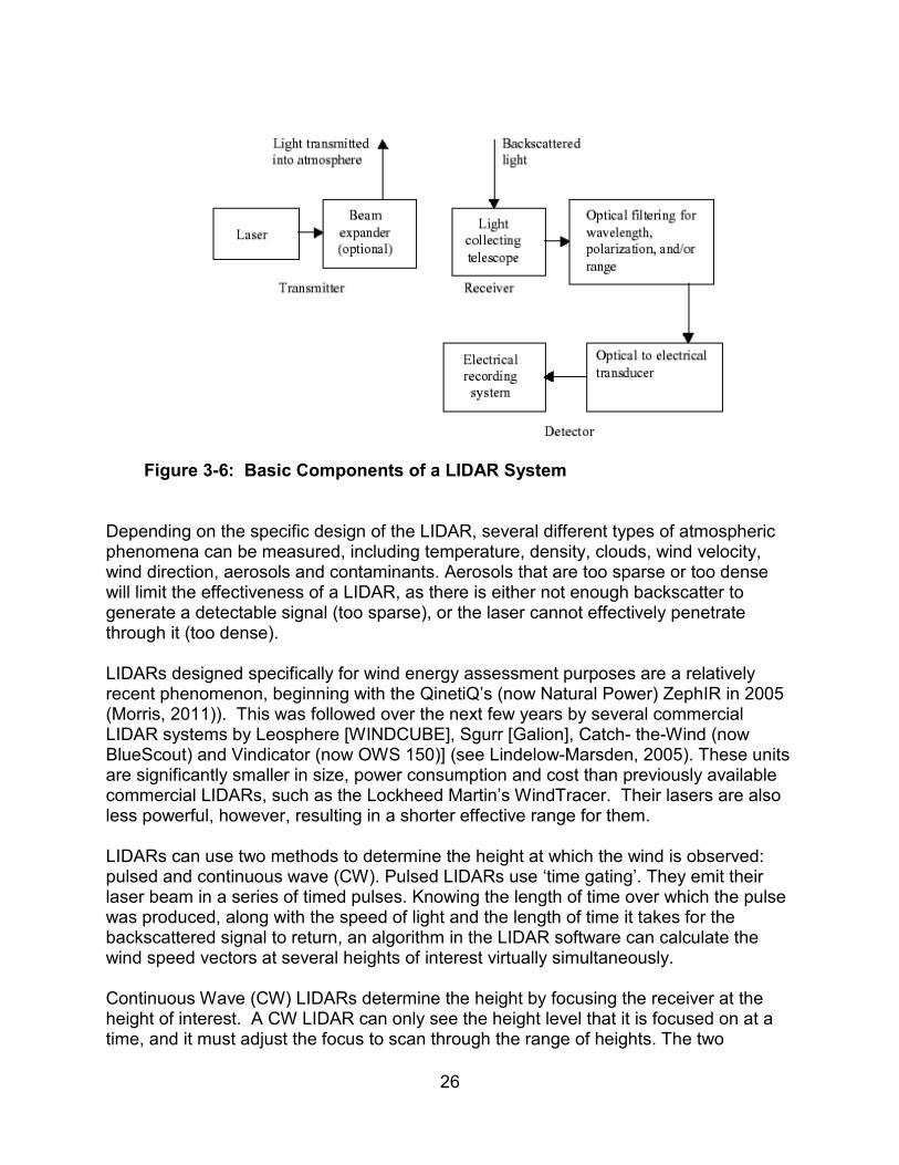
26

Depending on the specific design of the LIDAR, several different types of atmospheric phenomena can be measured, including temperature, density, clouds, wind velocity, wind direction, aerosols and contaminants. Aerosols that are too sparse or too dense will limit the effectiveness of a LIDAR, as there is either not enough backscatter to generate a detectable signal (too sparse), or the laser cannot effectively penetrate through it (too dense). LIDARs designed specifically for wind energy assessment purposes are a relatively recent phenomenon, beginning with the QinetiQ’s (now Natural Power) ZephIR in 2005 (Morris, 2011)). This was followed over the next few years by several commercial LIDAR systems by Leosphere [WINDCUBE], Sgurr [Galion], Catch- the-Wind (now BlueScout) and Vindicator (now OWS 150)] (see Lindelow-Marsden, 2005). These units are significantly smaller in size, power consumption and cost than previously available commercial LIDARs, such as the Lockheed Martin’s WindTracer. Their lasers are also less powerful, however, resulting in a shorter effective range for them. LIDARs can use two methods to determine the height at which the wind is observed: pulsed and continuous wave (CW). Pulsed LIDARs use ‘time gating’. They emit their laser beam in a series of timed pulses. Knowing the length of time over which the pulse was produced, along with the speed of light and the length of time it takes for the backscattered signal to return, an algorithm in the LIDAR software can calculate the wind speed vectors at several heights of interest virtually simultaneously. Continuous Wave (CW) LIDARs determine the height by focusing the receiver at the height of interest. A CW LIDAR can only see the height level that it is focused on at a time, and it must adjust the focus to scan through the range of heights. The two

Figure 3-6: Basic Components of a LIDAR System

27

methods have varying strengths and weakness. The most prominent features involve probe length and cloud sensitivity (Courtney, 2008; Morris, 2011). On a pulsed type LIDAR, a pulse of light traveling upward can be viewed as a volume with a distinct probe length. Its length does not change as it propagates through the air. When a CW LIDAR focuses in at a given height, the effective probe length is the length of the beam that is in focus. This makes the probe length of a CW LIDAR increase with height, thus giving a smaller probe length at lower heights, and a greater probe length at greater heights. For example the ZephIR CW LIDAR has a probe length of 0.07m at 10 m, and 7.7m at 100 m (Natural Power, 2012). The sensitivity of the CW LIDAR does not degrade with height as the focus is adjusted. However, clouds above the focus height can backscatter additional light, which can degrade the signal, biasing the measurement. The solution to this is a cloud detection algorithm, which detects the erroneous signal and subtracts it from the data (Morris, 2011). A continuous wave LIDAR with a cloud detection algorithm has the advantage of working on low-level clouds or fog. LIDARs, whether CW or pulsed, do not measure wind like a cup anemometer. Cup anemometers measure the scalar wind speed essentially at a single point in space. LIDARs, like SODARs, measure the wind in a volume, breaking the wind down into its vector components. The biases introduced by vector averaging and volume averaging must be understood in order to make useful comparisons between the two types of wind data. Clive (2008) found that the ratio of vector to scalar averages depends on “wind direction variability according to a Bessel function of the standard deviation of the wind direction during the averaging period”. LIDAR data generally correlates well with meteorological tower anemometry (Courtney et al, 2008; Jaynes, 2011; Hasager, 2007; Margulis, 2012) but only to the degree that the assumptions made are correct (Bradley, 2008a). Another distinction in LIDAR types is between vertical profilers and scanning types. A vertical profiler LIDAR measures the wind straight above the LIDAR, similar to the data one would get from a tower at that location. A scanning LIDAR is able to direct its laser beam from horizon to horizon, generating a 3D view of the wind field in the area around the LIDAR. A complete scan takes substantially longer than a vertical profiler type. Examples of a scanning type LIDAR include the Sgurr Galion and the LM WindTracer.

3.4.4 Offshore Wind Energy LIDAR Applications As noted in the recent review of Lang and McKeogh (2011) there have been numerous applications of LIDAR technology applied to onshore wind applications. Following a review of the world technical literature, the same can be said for LIDAR technology applied to offshore wind research and development. A summary of this work for a number of research, development, and technical organizations is given below.

28

1) GL Garrad Hassan

A. Jaynes and Jacquemin (2009) reviewed the use of LIDAR for offshore wind resource monitoring applications.

B. Kindler and Oldroyd (2010) reviewed the use of offshore LIDAR for the EU

project NORSEWinD (North Sea).

C. Jaynes and Landberg (2011) worked with AXYZ (WindSentinel floating LIDAR system) and Lockheed Martin on floating LIDAR motion compensation algorithms for offshore wind resource assessment.

2) DNV (GEC) Consultants This organization is just starting work on this subject. The latest papers are from 2011 and include the following:

A. Hughes (2011) discussed innovative methods for offshore wind resource assessment with emphasis on recommendations for offshore resource assessment that minimize uncertainty in a cost-effective manner. The author looked at data collection technologies that included: offshore meteorological mast, fixed platform remote sensing, remote sensing on floating platforms, buoys, and scanning LIDAR. This work also considered floating remote sensing- with no motion compensation. On this subject, the findings included: motion introduces greater scatter (at small timescales); scalar averages could be biased high; and, with motion compensation, instrument should be able to provide correct measurements. Recommendations included: use as stable a platform as possible to minimize tilt, an on-board 2-axis inclinometer could potentially be used to correct tilt bias, and any floating instrument needs a system for direction measurement.

B. Conover, et al (2011). This paper is a shortened version of the previous

presentation and refers to the next paper by Rogers. It does mention the use of long-range scanning LIDAR.

C. Rogers, et al (2011). This presentation specifically addresses remote sensing on

moving offshore platforms. It summarizes the advantages (lower cost than bottom-mounted tower, moveable from site to site) and the disadvantages (offshore reliability and maintenance access, power supply reliability and size) of such platforms.

3) DTU Risø (Danish National Laboratory for Sustainable Energy This well-established European research laboratory has been a pioneer in remote wind resource assessment and has performed numerous experiments and studies for SODAR and LIDAR systems- for both onshore and offshore applications. A majority of

29

their recent work on this subject has been sponsored by the European UpWind project that is investigating the design of wind turbines up to 20 MW in size. Papers of most interest include the following:

A. Joergensen, et al (2008) outlined the scope of their UpWind research on both SODAR and LIDAR systems.

B. Kindler, Courtney, and Oldroyd (2009) summarized the testing and calibration of

LIDAR systems for a 2 year offshore wind measurement program. The project was designed to serve as a benchmark test study so that future validation tests performed by researchers and industry could have a common basis of comparison.

C. Courtney (2010) reviewed the 2010 state-of-the-art of LIDAR systems for wind

measurement and summarized some of the problems of its use in complex terrain. Of interest in offshore applications, the author pointed out hidden or forgotten costs of LIDAR systems (Power supply, maintenance, and repairs)

D. Courtney (2011) in the final report of the UpWind project, gave a comprehensive

review of the state-of-the-art of LIDAR technology (and some SODAR developments) and presented a summary of projected future developments in remote sensing for wind energy applications. In addition to showing the latest Risø developments for LIDAR systems (see Figure 3-7), the following areas of interest for offshore wind applications were summarized: better LIDARS used less power and were less expensive: value of turbulence measurement with LIDARs; value of LIDARs mounted on wind turbines; and value of multiple LIDAR systems.

E. Wagner, et al. (2011) in the most recent EWEA Offshore Conference

summarized the results of an experimental program that investigated the performance of a nacelle mounted LIDAR system in the context of the current IEC testing standards (61400-12). The authors concluded that, subject to some minor deviations, nacelle LIDAR can be successfully used for wind turbine power curve measurement.

F. Pena, et al. (2011) summarized the results of long-term use of 4 platform

mounted LIDARs (WINDCUBE) in the North Sea for providing input to wind research and forecast (WRF) models.

30

4) University of Stuttgart/ AREVA (Germany) Researchers from the University of Stuttgart and AREVA wind in Germany have been investigating the performance of LIDAR systems with various enhancement systems (such as nacelle mounted systems) for both onshore and applications. A summary of their latest work includes the paper of Bischoff, et al. (2011). This paper summarizes the results of load analyses based on LIDAR data for the AREVA M5000 (5 MW) wind turbine. 5) 3E (Brussels) In a presentation at the 2011 EWEA Offshore Wind Conference, Duffey, et al. (2011) summarized their work on a floating LIDAR system that is based on a mechanical

Figure 3-7: Schematic of Risø Multi-Lidar System. (Courtney, 2011)

31

stabilization and software correction systems. Their system used Leosphere LIDAR technology. Unfortunately, few details of the stabilization and software systems are given in this paper. In another paper 3E researchers (Coppye et al, 2011) present the results of a case study showing the value of floating LIDAR systems for offshore wind farm development. 6) Grand Valley State University/ AXYZ Technologies In a presentation from the EWEA 2011 Offshore Wind Conference, Boezaart, Howe and Belen (2011) summarize the development of an offshore buoy system that features a LIDAR system. AXYZ Technologies provided the LIDAR instrumentation and the system was designed to be used for a Great Lakes Offshore wind feasibility study. 7) University of Strathclyde/ Oldbaum Services/ Risø DTU Strickland, et al. (2011a) present the results of a feasibility study using a WINDCUBE LIDAR for the determination of the offshore wind profile off an offshore platform. Another paper from this research group (Strickland, 2011b) compared the results of WINDCUBE and ZephIR LIDARs from the same platform. 8) Von Karman Institute for Fluid Dynamics, Belgium/Deutsches Windenergie-Institut GmbH Von Karman Institute researchers (Munoz-Esparza, et al., 2011) used a LIDAR system from the FINO 1 platform to measure a number of atmospheric characteristic properties. 9) DEWI GmbH- Deutsches Windenergie-Institut DEWI (see Neumann, et al. (2012) used a Leosphere WINDCUBE pulsed LIDAR on the FINO 1 offshore platform in order to measure wind profiles at the Alpha Ventus wind farm site (See Figure 3-8). They also carried out LIDAR experiments on a wind turbine nacelle and an offshore transformer substation. 10) Norwegian Researchers As summarized in the latest IEA Annex 32 proceedings (IEA, 2012), there is a considerable amount of offshore LIDAR research in Norway at the present time. This includes the following:

A. University of Bergen (Norway) and the Norwegian Center for Offshore Wind Energy (NORCOWE). At the University of Bergen, this work is being lead by Professor Joachim Reuder who has also noted that a LIDAR system in conjunction with Microwave temperature profiler looks interesting for stability studies. For the latest information on the NORCOWE activities see http://www.norcowe.no, and

http://www.norcowe.no/

32

http://www.norcowe.no/doc//Norges%20Forskningsr%C3%A5d/NORCOWE%20annual%20report%202011_low%20resolution.pdf

B. Norwegian Research Centre for Offshore Wind Technology (Nowitech). This organization has several international projects in offshore wind energy including a project for LIDAR based studies of offshore wind farm wakes (see http://www.sintef.no/projectweb/nowitech/)

C. The University of Agder. This organization is active in the use of offshore LIDAR.

Agder has two land-based, articulated 6 degree-of-freedom platforms for a variety of purposes. The smaller one carries 1.8 tons, the larger carries 6 tons. These platforms are useful for calibrating floating LIDARs. See http://www.youtube.com/watch?v=bJQWBHRlaMA. Agder also has two buoys with LIDARs, but they were damaged in storms.

Figure 3-8: LIDAR at FINO 1 Offshore Platform (Neumann et al, 2012)

http://www.norcowe.no/doc/Norges%20Forskningsr%C3%A5d/NORCOWE%20annual%20report%202011_low%20resolution.pdf

http://www.norcowe.no/doc/Norges%20Forskningsr%C3%A5d/NORCOWE%20annual%20report%202011_low%20resolution.pdf

http://www.sintef.no/projectweb/nowitech/

http://www.youtube.com/watch?v=bJQWBHRlaMA

33

3.4.5 Summary of Current Manufacturers and Specifications As recently as 2008, there were only about three LIDAR system manufacturers that specialized in instrumentation for wind assessment purposes (Courtney, 2008; Lindelow-Marsden, 2009). At the present time there are five well-established commercially available vertical-profiling LIDAR systems. They are shown in Figures 3- 9 to 3-11 and include the following manufacturers:

• Natural Power (Figure 3-9A) • Leosphere (Figure 3-9B) • Sgurr (Figure 3-10) • Catch the Wind/Vindicator (BlueScout) (Figure 3-10) • Lockheed Martin (Figure 3-11)

Figure 3-9: Left- Natural Power LIDAR System; Right- Leosphere WINDCUBE LIDAR System. (http://www.naturalpower.com/products), (http://www.leosphere.com/)

http://www.naturalpower.com/products

34

Figure 3-10: Sgurr (left) and Catch the Wind/Vindicator (BlueScout) LIDAR Systems (right). (http://www.sgurrenergy.com/galion-lidar/); (http://www.bluescout.com/products/BlueScoutOWS150)

Figure 3-11: Lockheed Martin LIDAR System. (http://www.lockheedmartin.com/us/products/windtracer.html)

http://www.sgurrenergy.com/galion-lidar/

http://www.bluescout.com/products/BlueScoutOWS150

35

The five manufacturers previously mentioned have carried out or sponsored a number of development programs on both onshore and offshore applications of LIDAR systems. Offshore use of LIDAR systems are summarized below. Natural Power: Natural Power’s CW LIDAR ZephIR (Natural Power, 2012) was initially developed in 2001 by QinetiQ, a UK research and development laboratory, and was released for commercial sales in 2003. Starting with the initial work on the ZephIR system at DTU Risø, Denmark’s national wind energy research center, there have been many onshore demonstrations and applications of this system. In 2007 Natural Power exclusively licensed the technology from QinetiQ to market ZephIR to the global market and to commence serial production. For offshore applications, the ZephIR LIDAR has been used at over 30 offshore sites, including the following (Smith, 2012):

o Beatrice Platform, North Sea (2005) o Horns Rev, North Sea (2006) o FINO 1, North Sea (2006) o NaiKun, Hecate Strait (2006) o Cleveland Crib, Great Lakes (2009) o FINO 3, North Sea (2010) o Robin Rigg, Solway Firth (2010) o Dogger Bank, North Sea (2011)

Leosphere: This pulsed beam LIDAR system (WINDCUBE) was developed in cooperation with the French Aerospace agency (ONERA). At the present time NRG and Leosphere are the distributors for the WINDCUBE system that has two commercial versions (Leosphere, 2012). This system has a number of recent offshore applications including the following:

o North Sea, Germany: In 2010 a one year LIDAR measurement test was carried out on the FINO 1 Platform (Westerhellweeg et al, 2010).

o Thevenoud et al. (2012) used a WINDCUBE on the FLIDAR buoy platform

o China: Guodian Corporation purchased a WINDCUBEv2 Offshore to evaluate the

wind resource twenty-five kilometers off the shores of China’s Shandong Province, in the Yellow Sea.

Sgurr: The Sgurr Galion Pulsed beam LIDAR system was tested by Risø Laboratories in 2009 (Gottschall et al, 2009) and has been deployed in a number of onshore sites. The current product line is considered as a second generation LIDAR system (Clive, 2009) and is available in onshore and offshore versions. As summarized by Clive (2011), this type of remote sensing can be used for significant advantage in offshore wind energy projects. In 2012, in cooperation with the German Wind Energy Institute, DEWI, a Galion LIDAR system was deployed on FINO 1 in the German North Sea. In

36

addition, Sgurr Energy has been commissioned by Hong Kong Electric Company, to deploy Asia’s first LIDAR device for capturing wind speed and directional data in an offshore environment. Catch the Wind/ Vindicator: This pulsed beam LIDAR system developed by Catch the Wind (Vindicator) was originally developed for real time control using a nacelle mounted LIDAR measurement system. The Vindicator LIDAR uses platform motion correction algorithms based on its original use for wind shear sensing aboard in-flight helicopters. This has led to its incorporation in the WindSentinel buoy marketed by AXYS Technologies in British Columbia (see section 3.5.10). Catch the Wind has recently been acquired by BlueScout Technologies (BlueScout, 2012). Lockheed Martin: The WindTracer LIDAR system is the only commercial system for long-range volume scanning (Lockheed, Martin, 2012). It was originally developed for wind shear monitoring at airports (Lerner, 2002). As described in the publication of Hannon (2009), the WindTracer has demonstrated clear-air effective ranges of 15-25 km. In November 2011, a team of Fishermen’s Energy engineers and specialists from Lockheed Martin installed a WindTracer LIDAR on the rooftop of a seaside apartment building in Margate, New Jersey. The system is used for wind resource assessment of two off-shore wind farms: one at 2.8 miles off the coast of Atlantic City, in New Jersey state waters and the second at 10 miles off shore in Federal water (Lockheed Martin, 2011). For potential offshore wind monitoring applications, the summary in Table 3.2 lists the commercial LIDAR systems that could be mounted on fixed platforms and Table 3.3 summarizes the systems that could be mounted on floating platforms. This summary, which should not be considered exhaustive due to the rapid expansion of models, has identified 5 separate manufacturers making distinct LIDAR systems, 4 fixed and 4 floating. As shown, there are many LIDAR design options, including laser modes (pulsed vs. continuous wave), configuration (single, three, four, and five beam systems), and vertical profile vs. scanning LIDARs. At the present time no one design philosophy predominates, suggesting that the field is still in a degree of flux and growth. For the design of complete systems, in addition to weight and volume specifications, the power requirements of the LIDAR systems are major design variables that must be considered. For example, as shown for floating platforms, the power requirements can range from 45 to 250 watts. A summary of existing LIDAR offshore wind monitoring applications will be presented in the next section.

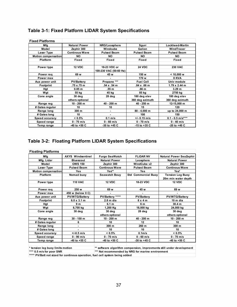
37

Table 3-1: Fixed Platform LIDAR System Specifications

Table 3-2: Floating Platform LIDAR System Specifications

Fixed PlatformsMfg Natural Power NRG/Leosphere Sgurr Lockheed-Martin

Model Zephir 300 Windcube Galion WindTracerLaser Type Continous Wave Pulsed Beam Pulsed Beam Pulsed Beam

Motion compensation NO NO NO NOPlatform Fixed Fixed Fixed Fixed

Power type 12 VDC 18-23 VDC or 24 VDC 230 VAC100-230 VAC (50-60 Hz)

Power req 69 w 45 w 150 w < 10,000 wPower max - - 170 w 8 KVA

Aux power unit PV/Battery Propane *** Fuel Cell Univ module Footprint .75 x.75 m .54 x .54 m .84 x .66 m 1.79 x 2.44 m

Hgt 0.85 m .55 m .66 m 3.29 mWgt 55 kg 45 kg 85 kg 2750 kg

Cone angle 30 deg 28 deg 180 deg elev 180 deg elevothers optional 360 deg azimuth 360 deg azimuth

Range reg 10 - 200 m 40 - 200 m 40 - 250 m 12-15,000 m# Gates regular 10 10 15 120

Range long 300 m - 80 - 4,000 m up to 24,000 m# Gates long 10 - 100 150

Speed accuracy < 0.5% 0.1 m/s +/- 0.15 m/s 0.1 - 0.5 m/s****Speed range 0 - 70 m/s 0 - 60 m/s 0 - 70 m/s 0 - 40 m/sTemp range -40 to +50 C -30 to +45 C -15 to +35 C -20 to +40 C

Floating PlatformsMfg AXYS Windsentinel Furgo SeaWatch FLiDAR NV Natural Power SeaZephir

Mfg, Lidar Bluescout Natural Power Leosphere Natural PowerModel OWS 150 Zephir 300 WindCube v2 Zephir 300

Laser Type Pulsed Beam Continous Wave Pulsed Beam Continous WaveMotion compensation Yes Yes** Yes Yes*

Platform Nomad buoy Seawatch Bouy Std Commercial Buoy Tension Leg Buoy20m min water depth

Power type 110 VAC 12 VDC 18-23 VDC 12 VDC

Power req 250 w 69 w 45 w 69 wPower max 450 w (below 0 C) - - -

Aux power unit PV/WTG/Battery PV/Battery ***** PV/Battery PV/WTG/BatteryFootprint 6.0 x 3.1 m 2.8 m dia 8 x 4 m 10 m dia

Hgt 9 m 6.1 m 6 m 30.4 mWgt 8,700 kg 1,200 Kg 18,000 kg 24,000 kg

Cone angle 30 deg 30 deg 28 deg 30 degothers optional others optional

Range reg 30 - 150 m 10 - 200 m 40 - 200 m 10 - 200 m# Gates regular 6 10 12 10

Range long - 300 m 260 m 300 m# Gates long - 10 10 10

Speed accuracy +/-0.5 m/s < 0.5% 0.1m/s < 0.5%Speed range 0 - 90 m/s 0 - 70 m/s 0 - 60 m/s 0 - 70 m/sTemp range -40 to +55 C -40 to +50 C -30 to +45 C -40 to +50 C

* tension leg buoy limits motion ** software algorithm compension, improvments still under development **** 0.5 m/s for poor SNR *** Not recommended by NRG for marine environment***** PV/Batt not sized for continous operation, fuel cell system being added

38

3.5 Potential Sea Platforms for Instrumentation Based on past experience, installing an offshore platform at sea for wind assessment purposes can be a multi-million dollar expense with a range of $2.5 – 10 million dollars US (Nordman, 2012). This is a significant startup cost; much more than typically seen on a land based study. For example, if the subsequent wind data suggests relocating either the study area or the platform location itself, then moving that platform essentially means starting over (BTT Marine, 2011-2012). The offshore terrain may appear quite uniform, but shore effects can be detected in the wind profiles even miles out to sea (Hasager, 2007). As such, lower expense alternatives to a permanent offshore platform ought to be carefully considered when the option(s) are available. Thus, the following sections will review both fixed platform LIDAR systems as well as floating platform systems.

3.5.1 Fixed Platforms As will be discussed below, fixed platforms that were considered in this work include the following:

• Long term platforms • Short term platforms • Nearby islands • Re-tasking existing offshore structures • Coastal onshore locations

3.5.2 Long Term Platforms

Typical offshore monitoring platforms are steel or concrete structures anchored to the seabed by piles or gravity caisson. Depending on the size and type of equipment carried (meteorological tower, LIDAR, helipad, etc.) the deck size can be quite large. The technology is well established, but costly (Nordman, 2012). Platforms can be used in both shallow and deeper waters. As shown in Figure 3-12, examples include the Cape Wind meteorological tower (left) and the Naikun tower off Vancouver, BC (right).

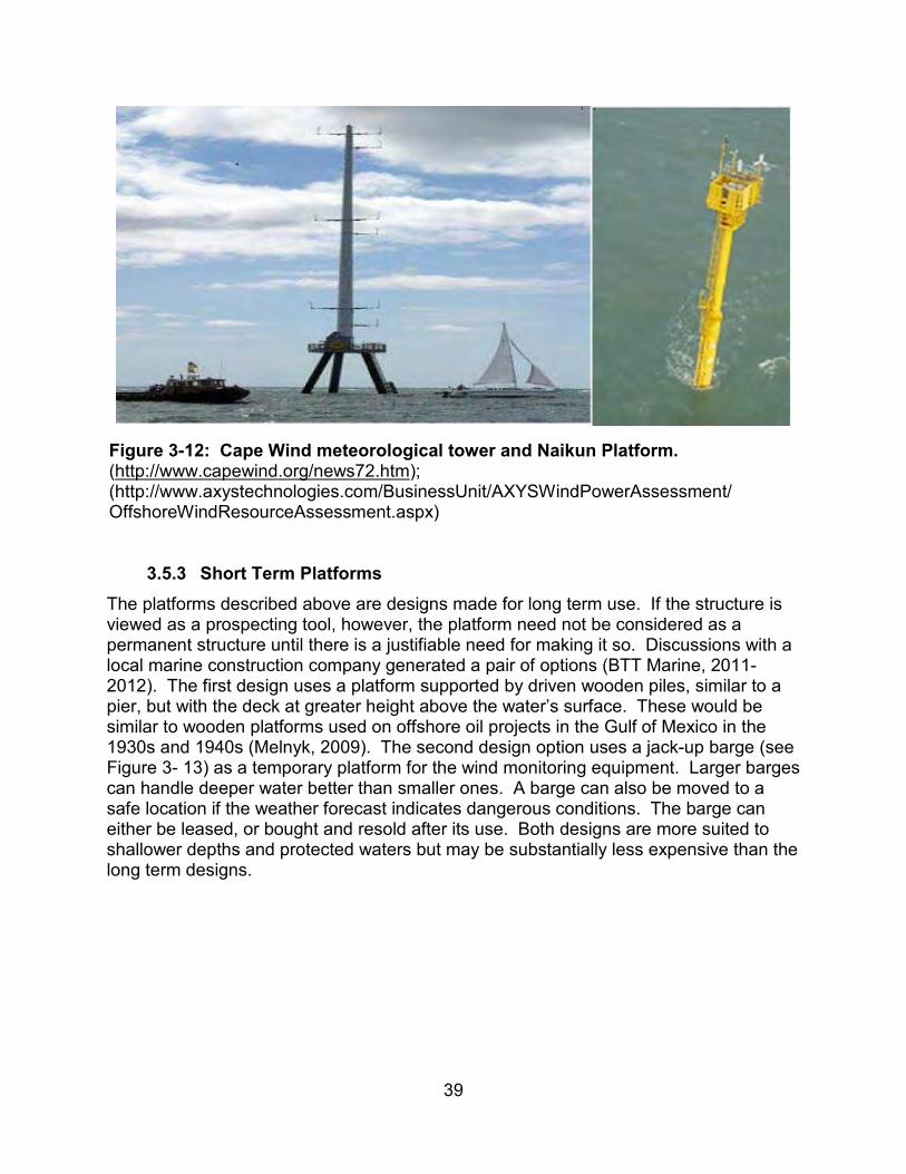
39

3.5.3 Short Term Platforms

The platforms described above are designs made for long term use. If the structure is viewed as a prospecting tool, however, the platform need not be considered as a permanent structure until there is a justifiable need for making it so. Discussions with a local marine construction company generated a pair of options (BTT Marine, 2011-2012). The first design uses a platform supported by driven wooden piles, similar to a pier, but with the deck at greater height above the water’s surface. These would be similar to wooden platforms used on offshore oil projects in the Gulf of Mexico in the 1930s and 1940s (Melnyk, 2009). The second design option uses a jack-up barge (see Figure 3- 13) as a temporary platform for the wind monitoring equipment. Larger barges can handle deeper water better than smaller ones. A barge can also be moved to a safe location if the weather forecast indicates dangerous conditions. The barge can either be leased, or bought and resold after its use. Both designs are more suited to shallower depths and protected waters but may be substantially less expensive than the long term designs.

Figure 3-12: Cape Wind meteorological tower and Naikun Platform. (http://www.capewind.org/news72.htm); (http://www.axystechnologies.com/BusinessUnit/AXYSWindPowerAssessment/ OffshoreWindResourceAssessment.aspx)

http://www.capewind.org/news72.htm

40

3.5.4 Nearby Islands In the case where an island is nearby to the study area, it may be useful to locate the LIDAR there. In coastal New England, there are several potential islands that could be of use to various wind projects. For example, as shown in Figure 3-14, Little Brewster, one of the harbor islands of Boston, is home to Boston Light, the last manned USCG lighthouse in the United States. It is about 2.5 miles from Hull, Massachusetts, a town that has considered building an offshore wind park. Electric power is available and the UMass Wind Energy Center once used the site for testing a ZephIR/Natural Power LIDAR.

Figure 3-13: Jack-up Barge (http://www.pajot.com/product/jack-up-barge/)

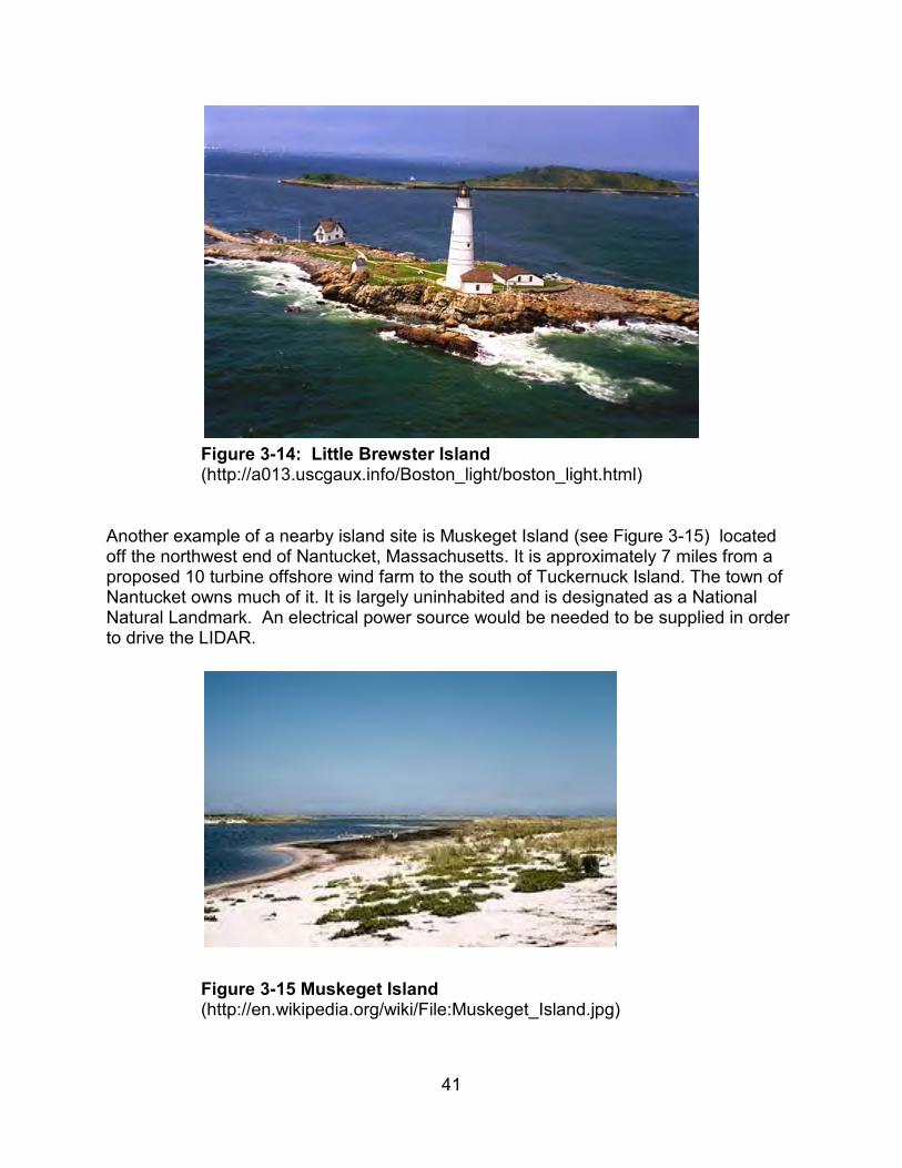
41

Another example of a nearby island site is Muskeget Island (see Figure 3-15) located off the northwest end of Nantucket, Massachusetts. It is approximately 7 miles from a proposed 10 turbine offshore wind farm to the south of Tuckernuck Island. The town of Nantucket owns much of it. It is largely uninhabited and is designated as a National Natural Landmark. An electrical power source would be needed to be supplied in order to drive the LIDAR.

Figure 3-14: Little Brewster Island (http://a013.uscgaux.info/Boston_light/boston_light.html)

Figure 3-15 Muskeget Island (http://en.wikipedia.org/wiki/File:Muskeget_Island.jpg)

42

3.5.5 Re-tasking an Existing Offshore Structure

Offshore structures, originally constructed for other purposes, may sometimes be used as platforms for deploying LIDARs. For example, the Woods Hole Oceanographic Institution maintains an offshore research structure located approximately 1.6 miles south of Martha’s Vineyard. It is well suited to host some of the smaller LIDARs, with electric power available on the platform. It was designed to be a minimal cost, rapid deployment time structure, so the design can also be considered as a potential short term platform template (Gaythwaite and Mellor, 2004). As previously discussed, in 2005, the UMass Wind Energy Center tested an ART VT-1 SODAR at this location (see Figure 3-16). The echo that bounced off the meteorological mast limited the SODARs effectiveness. A LIDAR would not have had that problem because the laser can be oriented away from the mast.

There are other existing ocean-based structures, but not all of them are so well suited to be used without significant modifications. Two possible locations are the Cape Wind meteorological tower, mentioned earlier, and the Bishop and Clerks lighthouse, south of Hyannis, MA (see Figure 3-17). At the present time, both lack sufficient deck space for both the LIDAR and for a power supply needed to provide electricity.

Figure 3 - 16: ART VT-1 at WHOI platform. (UMass photo)

43

3.5.6 Coastal Onshore Location

If the study area is not too far offshore, an onshore location may become suitable for the LIDAR. What can be considered ‘too far’ is a function of which type LIDAR is used. A vertical profiling LIDAR needs to be close to the target area, while scanning LIDAR can reach out and directly measure the site, up to 15 km in the case of the WindTracer.

3.5.7 Floating Platforms When suitable monitoring sites cannot be found, whether onshore, on an island, or on an existing platform, one has to be constructed. One of the more recent developments in the technology has been designing floating structures to support the LIDARs on station. At the present time four different designs are currently available or completing the final testing stages (Nordman, 2012; Jaynes, 2011a; Jaynes 2011b; Courtney, 2012; CMR and Univ. of Bergen, 2012). Three of the designs use a motion correcting algorithm to stabilize the scans the LIDAR makes. Details of the motion correction algorithms are all proprietary: only the results of said compensation tests are available. The fourth buoy design relies on an inherently stable tension-leg design to control its motion so there is no need to correct for motions. All of these are capable of being operated in deeper waters than the existing meteorological tower platforms currently in use. As described below, these four are:

Figure 3-17: Bishop & Clerks Lighthouse (UMass photo)

44

• SeaZephIR • AXYS WindSentinel • FLiDAR • Fugro

3.5.8 SeaZephIR The SeaZephIR, shown in Figure 3-18 uses a tension-leg buoy to support a ZephIR 300 LIDAR. Power is supplied by solar panels, wind turbines and battery setup. In extreme sea states, if the motion exceeds tolerated limits, the data is marked as such. That data is either rejected outright or will have a lower quality rating assigned to it. This system is the heaviest of the four designs. It includes a gravity type anchoring system. The SeaZephIR is currently available for deployment. For example, such a system was installed off the New Jersey coast in November of 2012 (North American Windpower, 2012).

Figure 3-18: SeaZephIR (http://www.searoc.com/index/99/News)

45

3.5.9 AXYS WindSentinel The AXYS WindSentinel uses a BlueScout OWS-150 LIDAR paired with a Nomad buoy. Nomad is a standard buoy design with a long operational history, and is boat-like in appearance (see http://www.ndbc.noaa.gov/mooredbuoys.html). The OWS-150 has a built-in motion correction algorithm. Power is supplied by a combination of solar, wind and batteries. This system, shown in Figure 3-19, is currently available for deployment.

3.5.10 FLiDAR The FLiDAR (Figure 3-20) uses a Leosphere WINDCUBE v2 for its LIDAR system (see Douglas, 2012). A motion correction algorithm was specifically developed for the WINDCUBE for this system. The buoy itself is of a standard commercial design. Like the previous two LIDAR systems, power is supplied by a combination of solar, wind and batteries. Sea trials were completed in the North Sea off the coast of Belgium in late 2011and the system was validated in May 2012 (Courtney, 2012). It is commercially available for deployment.

Figure 3-19: AXYS WindSentinel (http://www.axystechnologies.com/BusinessUnit/ AXYSWindPowerAssessment/OffshoreWindResourceAssessment/ WindSentinel.aspx)

http://www.ndbc.noaa.gov/mooredbuoys.html

http://www.axystechnologies.com/BusinessUnit/

46

3.5.11 Fugro Seawatch

The Fugro Seawatch uses a ZephIR 300 LIDAR, the same as in the SeaZephIR. It is paired with a SeaWatch buoy (Figure 3-21), a standard commercial design. The first test was done without a motion correcting algorithm, but the manufacturer has more recently been testing a compensating algorithm to see if it can improve the results (CMR/Univ. of Bergen, 2012; Mathisen, 2012). The buoy is the smallest and lightest of the four floating designs, but currently is not capable of long deployments because it has an undersized solar and battery power supply. The manufacturer intends to add a fuel cell power plant to the package, which will require periodic boat trips to refuel, unlike the other three buoy systems. Accordingly, it cannot be utilized as a long-term wind assessment tool at present, but it should be considered again when the design is more mature and tested.

Figure 3-20: FLiDAR Buoy (Courtney et al, 2012)

Figure 3-21: Fugro SeaWatch LIDAR Buoy (http://renews.biz/fugro-launches-new-lidar-buoy-2/)

47

3.6 Recommendations/Conclusions Based on this review, the following conclusions and recommendations may be made: 1) LIDAR is a better choice for offshore wind and direction measurements than SODAR: The researchers first concluded that balloons and UAVs systems are not available for long-term offshore data acquisition. In general, SODAR systems have greater scatter (e.g., standard deviation) referenced to cup anemometry than LIDARs. That is, LIDARs have been tested in various manners against cup anemometry and can give good service in the simple terrain environments expected offshore. Most importantly, no commercial SODAR has been given a motion compensation system suitable for a floating structure, so they must be based on either a fixed platform ($2.5-10 million) or on land. Also, as previously discussed, the UMass offshore experience with ART VT-1 SODAR at the WHOI platform was not successful - the SODAR was affected by wind passing through the base structure or noise from waves breaking on the structure. 2) For LIDAR systems the required power and other system factors are important: As noted in this review there is a large variation (45W to 10KW) in the power requirements for commercially available LIDAR systems. For example, for offshore platform systems, the Fugro Seawatch power supply, due to its short battery life, is not now suitable until the manufacturer installs a fuel cell (estimated for 2014) to power it (currently only a week or so on batteries). In any case, the fuel cell would require periodic refueling, unlike the PV/Battery/WTG systems that the other floating LIDARS use. The Seawatch is, however, the lightest buoy design and probably the most easily deployable. 3) Different locations should be considered for offshore LIDAR system measurements: Just one type of LIDAR does not fit all possibilities. Thus, one has to decide what kind of LIDAR to use and where to locate it (between near onshore and floating). For near onshore the Galion LIDAR has a relatively short range as compared to (the much more expensive) Lockheed- Martin WindTracer system. Thus, a good system for distances close to shore would be a land based scanning LIDAR (Galion – up to 4 km /WindTracer – up to 15 km). Also, if one has to put up a multimillion dollar platform, one might as well go with a mast plus a floating LIDAR. Furthermore, the WindTracer has very high power requirements in relation to the others, and it should be kept on land. Its ability to see the whole field of view is preferred, but the long time to complete a full scan means that the data has to be a bit more pixelated than what a vertical profiler would show at the same location. 4) For far offshore LIDAR applications, where floating systems would be used, no clear choice is apparent: There is no clear choice in terms of quality of data between the SeaZephIR and the SeaWatch systems. The SeaZephIR and SeaWatch can be deployed as needed in water depths up to their anchoring limitations. Further out from shore- there is not strong preference. The SeaZephIR, having a tension leg design, must be deployed in deeper waters (20 m min) than the others, so is more limited in where it can go. Since the tension leg design eliminates the need for motion compensation algorithms, it is simpler than the others (lower risk?). It is however,

48

massively heavy due to the 220 tonne anchor system, so one would not want to move it around very often. A question that must be answered– can a tension leg design be stable enough for a scanning LIDAR? If so, how long a range is possible before an algorithmic software correction would be needed? 5) LIDAR systems are still in a period of technical improvement: At the present time the wind system measurement LIDAR technology is constantly changing, hopefully gaining more reliability, requiring less operational expertise and maintenance along with improved (lower power) power supplies. In addition, testing, validation, and standards development are under way in many detailed studies (e.g., via IEA Wind Annex 32 work).

49

3.7 References Antoniou, I, Jorgensen, A., Ormel, F., Bradley, S., von Hunnerbein, S., Emeis, S., and

Warmbier, G. (2003) “On the Theory of SODAR Measurement Techniques”, Risø National Laboratory report Risø-R-1410(EN).

Antoniou, I., Jorgensen, A., Mikkelsen, T., Frandsen, S., Barthelmie, R., Perstrup, C.,

and Hurtig, M. (2006) “Offshore wind profile measurements from remote sensing instruments”, EWEC 2006 (Athens, Greece).

Argall, P. S. and Sica, R. J. (2002) “Lidar” in Encyclopedia of Imaging Science and

Technology, Wiley Barthelmie, R., Folkerts, L., Ormel, F., Sanderhoff, P., Eecen, P., Stobbe, O., and

Nielsen, N. (2003) “Offshore Wind Turbine Wakes Measured by SODAR”, Journal of Atmospheric and Oceanic Technology, 20.

Berg, A. (2006) “The feasibility of sodar wind profile measurements from an

oceanographic buoy” MS Thesis: Woods Hole Oceanographic Institute/ MIT. Bischoff, O., Anger, J., Hofsaess, M., Rettenmeler, A., Schlipf, D., and Siegmeier, B.

(2011) “Vertical Wind Shear Measured with a Nacelle-Based LIDAR system and its Impact on Mechanical Loads,” Proc. 2011 EWEA Offshore Wind Conference.

BlueScout, (2012) BlueScout Technologies, Internet: http://www.bluescout.com/,

accessed Dec. 31, 2012. Boezaart, T. A. Howe, G., and Belen, F. (2011) “Implementing Offshore Remote Wind

Sensing Technologies including Protocols for the Evaluation, Selection, and Validation,” Proc. 2011 EWEA Offshore Wind Conference.

Bradley, S. (2008a) “Wind Speed Errors for LIDARs and SODARs in Complex Terrain”,

IOP Conference series: Earth Environ. Sci. 1 01261 (Risø DTU 2008) Bradley, S. (2008) Atmospheric Acoustic Remote Sensing, CRC Press, Boca Raton, FL. BTT Marine (2011-2012) Personal Communication, East Boston MA. Clive, P. (2008) “Compensation of Bias in Lidar Wind Resource Assessment, Wind

Engineering” 32, no. 5. Clive, P. (2009) “Wind Monitoring Using 2nd Generation Wind Lidars, Wavenet

Conference Proceedings, Internet: http://www.wakenet3-europe.eu/index.php?id=125&no_cache=1&type=98, accessed December 31, 2012.

http://www.bluescout.com/

http://www.wakenet3-europe.eu/index.php?id=125&no_cache=1&type=98

http://www.wakenet3-europe.eu/index.php?id=125&no_cache=1&type=98

50

Clive, P. (2011) “Remote Sensing Standards: Their Current Status and Significance for Offshore Projects,” Proc. EWEA 2011. Internet: http://www.sgurrenergy.com/wp-content/uploads/2012/12/Industry-paper-Remote-sensing-standards-their-current-status-and-significance-for-offshore-projects.pdf, accessed December 31, 2012.

CMR and Univ. of Bergen (2012) “Measurements of Wind Profile from a Buoy Using

LIDAR – Final Report”, ref 9631/R0/05-06-2012 (June). Conover, K., Randall, G., Briggs, K., Hughes, H., Rogers, T., and Martin, V. (2011)

“Innovative Methods for Offshore Wind Resource Assessment,” Proc. EWEA 2011.

Coppye, W., Kyriazis, A., Mijlemans, L., and Duffey, T. (2011) “Case Study: The Value

of Floating LIDAR Technology During the Different Phases of Offshore Wind Farm Development,” Proc. 2011 EWEA Offshore Wind Conference.

Courtney, M., Wagner, R., and Lindelow, P. (2008) “Commercial Lidars for Wind

Energy, a Comparative Guide”, EWEC 2008, Brussels. Courtney, M. (2010) “Wind lidars- Not the final answer in complex terrain,” Proc. Ice and

Rocks 3, May 6. Courtney, M. (2011) “UpWind WP6- Remote Sensing Final Report- Deliverable D6.17,

RISO Technical Report Contract No. 019945(SE56). Courtney, M. and Wagner, R. (2012) “Validating the 3E FLiDAR’, DTU Wind Energy

VindKraftNet Meeting (Lyngby), May. Douglas, B. (2012) “ Floating Lidar Wind Measurement,” Windtech International,

Jan/Feb, p7. Duffey, T., Devriendt, D., Guidon, N., KyriaZis, T., and Picot, N. (2011) “Validated

Measurements of a Floating LIDAR Device Based on Mechanical Stabilization and Software Correction”, Proc. Offshore EWEA 2011.

Environmental Monitor (2012) “Buoys may best towers in offshore wind assessments”

Internet: http://www.fondriest.com/news/buoys-may-best-towers-in-offshore-wind-assessments.htm (Accessed September 20, 2012).

Gaythwaite, J. W. and Mellor, D. C. (2004) “Design of an Offshore Tripod Structure for

MET/OCEAN Research”, ASCE publication Ports 2004: Port Development in a Changing World.

Giebel, G., Bange, G. and Reuder, J. (2010) “Autonomous Aerial Sensors for Wind

Power Meteorology,” Proc. EWEA 2010.

http://www.sgurrenergy.com/wp-content/uploads/2012/12/Industry-paper-Remote-sensing-standards-their-current-status-and-significance-for-offshore-projects.pdf



http://www.fondriest.com/news/buoys-may-best-towers-in-offshore-wind-assessments.htm

http://www.fondriest.com/news/buoys-may-best-towers-in-offshore-wind-assessments.htm

51

Gottschall, J., Lindelöw-Marsden, P., Courtney, M. (2009) “Executive summary of key

test results for SgurrEnergy Galion” Risø Report, July 14, Internet: http://www.sgurrenergy.com/wp-content/uploads/2012/08/Riso_ExecutiveSummary_-Galion_lidar.pdf, accessed December 31, 2012.

Hannon, S. M. (2009) “Wind Resource Assessment Using Long Range Pulsed Doppler

Lidar,” Proc. 15th Coherent Laser Radar Conference, Toulouse, France. Internet: http://www.meteo.fr/cic/meetings/clrc/Hannon.pdf, accessed Dec. 31, 2012.

Hasager, C., Pena, A., Mikkelsen, T., Courtney, M., Antoniou, I., Gryning, S-E., Hansen,

P., and Sorensen, P. (2007) “12 MW Horns Rev Experiment”, Riso-R-1506(EN) Oct.

Hasager, C., Pena, A., Christiansen, M., Astrup, P., Nielsen, M., Monaldo, F.,

Thompson, D., and Nielsel, P. (2008) “Remote Sensing Observation Used in Offshore Wind Energy”, IEEE Journal 1, No 1.

Hughes, H. (2011), “Innovative Methods for Offshore Wind Resource Assessment,” DNV Presentation, Internet: http://www.all-energy.co.uk/userfiles/file/holly-hughes-190511.pdf, accessed 9/5/11.

IEA (2012) Proceedings of IEA Annex 32 LIDAR: Wind LIDAR Systems for Wind

Energy Deployment Meeting 2: at ForWind, University of Oldenburg, Germany, November 5-6.

Iowa Alliance for Wind Innovation and Novel Development (2012) “Iowa Alliance for

Wind Innovation and Novel Development Provides $300,000 Research Grant to Iowa State University” Internet: http://www.iawind.org/news-events/grant-isu-takle.pdf (Accessed September 20, 2012).

Jaynes, D. (2011) “LIDAR Lends a Hand in Resource Assessment”, North American

Windpower Supplement (Summer 2011)

Jaynes, D. and Jacquemin, J. (2009) “Exploring LIDAR Remote Sensing Technology for Offshore Wind Resource Monitoring Applications,” Proc. AWEA Annual Meeting.

Jaynes, D. and Landberg, L. (2011), Investigating the Efficacy of Floating LIDAR Motion

Compensation Algorithms for Offshore Wind Resource Assessment Applications,” Proc EWEA 2011.

Jaynes, D. (2011a) “Investigating the Efficacy of Floating Lidar Motion Compensation

Algorithms for Offshore Wind Resource Assessment Applications”, EWEC 2011 (Brussels, Belgium)

http://www.sgurrenergy.com/wp-content/uploads/2012/08/Riso_ExecutiveSummary_-Galion_lidar.pdf

http://www.sgurrenergy.com/wp-content/uploads/2012/08/Riso_ExecutiveSummary_-Galion_lidar.pdf

http://www.meteo.fr/cic/meetings/clrc/Hannon.pdf

http://www.all-energy.co.uk/userfiles/file/holly-hughes-190511.pdf

http://www.all-energy.co.uk/userfiles/file/holly-hughes-190511.pdf

http://www.iawind.org/news-events/grant-isu-takle.pdf

http://www.iawind.org/news-events/grant-isu-takle.pdf

52

Jaynes, D. (2011b) “LIDAR Lends a Hand in Resource Assessment”, North American Windpower Supplement (Summer)

Joergensen, H. E., Courtney, M., Mikkelsen, T., and Antoniou, A. (2008) “UpWind Progress in Remote Sensing of the Wind using LIDARS and SODARS, Proc. EWEA 2008.

Kadygrov, E. (2008) “Operational Aspects of Different Ground-Base Remote Sensing

Observed Techniques for Vertical Profiling of Temperature, Wind, Humidity, and Cloud Structures: A Review” World Meteorological Organization Report WMO/TD-No. 1309.

Kindler, D, Courtney, M., and Oldroyd, A. (2009) “Testing and Calibration of Various

LIDAR remote sensing devices for a 2 year Offshore Wind Measurement Campaign,” Proc. EWEWC 2009.

Kindler, D. and Oldroyd, A. (2010) “NORSEWinD: First Offshore LIDAR Deployments,”

Proc EWEA 2010. Kocer, G., Monsour, M, Chokani, N., and Abhari, R. S. (2011) “Full-Scale Wind Turbine

Near Wake Measurements Using an Instrumented Uninhabited Aerial Vehicle” ASME J. of Solar Energy Engineering, 133, No. 4.

Lang, S. and McKeogh, E. (2011) “LIDAR and SODAR Measurements of Wind Speed

and Direction in Upland Terrain for Wind Energy Purposes,” Remote Sensing, 3, PP1871-1901.

Leosphere, (2012) “Scanning Doppler Radar Lidar Systems” Internet:

http://www.lidarwindtechnologies.com/file_bdd/1334336572_windcube100s200s.pdf, accessed December 31, 2012.

Lerner, E. J. (2002) “Laser gyros, lidars guide air and space craft,” OptoIQ, April 1.

Internet: http://www.laserfocusworld.com/articles/print/volume-38/issue-4/features/laser-gyros-lidars-guide-air-and-space-craft.html, accessed Dec. 31, 2012.

Lindelow-Marsden, P. (2005) ‘Five Years of Lidar Anemometry in the Wind Energy

Industry – from Prototype to IEC Standard’, Risø DTU. Lockheed Martin (2011) “WindTracer Updates,” Dec. Internet:

http://www.lockheedmartin.com/us/products/windtracer/windtracerupdates.html (Accessed December 31, 2012)

http://www.lidarwindtechnologies.com/file_bdd/1334336572_windcube100s200s.pdf

http://www.lidarwindtechnologies.com/file_bdd/1334336572_windcube100s200s.pdf

http://www.laserfocusworld.com/articles/print/volume-38/issue-4/features/laser-gyros-lidars-guide-air-and-space-craft.html

http://www.laserfocusworld.com/articles/print/volume-38/issue-4/features/laser-gyros-lidars-guide-air-and-space-craft.html

http://www.lockheedmartin.com/us/products/windtracer/windtracerupdates.html

53

Lockheed Martin (2012) “WindTracer Lidar” Internet: http://www.lockheedmartin.com/content/dam/lockheed/data/space/documents/windtracer/WindTracer_Wind%20Energy.pdf (Accessed December 31, 2012).

Manwell, J.F., McGowan, J. G. and Rogers, A.R. (2009) Wind Energy Explained: Theory, Design and Application, Wiley, Chichester, UK.

Margulis, M. (2008) “WindTracer LIDAR and Wind Forecasting” Internet:

http://www.arpa-e.energy.gov/Portals/0/Documents/ConferencesAndEvents/PastWorkshops/Emerging%20Ideas/Improved%20wind%20and%20solar/Margulis_Presentation_ARPA-E_20120330.pdf (Accessed September 21, 2012)

Mathisen, J. (2012) Personal Communications with Manager of Seadata, Oceanor

(August) Melnyk, M. and Anderson, R. (2009) “Offshore Power: Building Renewable Energy

Projects in US Waters”, PennWell Books. Morris, L. (2011) “Second Generation LIDAR Boosts Wind Power”, Power Engineering,

Feb.

Munoz-Esparza, D., Canadillas, B., Neumann, T., and vanBeeck, J. (2011) “WRF Mesoscale Modelling and LIDAR Measurements of tall wind profiles at FINO 1,” Proc. 2011 EWEA Offshore Wind Conference.

Natural Power. (2012) “ZephIR” Internet: http://www.zephirlidar.com/, accessed

December 31, 2012) Neumann, T., Kinder, F., Canadillas, B, and Westerhellweg, A.. (2012) “Investigation of

wind flow disturbances by offshore wind turbines based on LIDAR measurements,” Proc. EWEA 2012.

(NOAA 2011)”NOAA Using Balloons to Capture Wind Data from Texas Wind Farm”

Internet http://www.nawindpower.com/e107_plugins/content/content.php?content.8537, accessed September 15, 2012.

Nordman, E. (2012) “Evaluating Offshore Wind Resources and Ecological Conditions in

Lake Michigan with a NOMAD buoy and laser sensor,” Proc. 2012 AWEA Annual Conference, Atlanta.

North American Windpower (2012) “SeaRoc Installs Floating Offshore Wind LIDAR

System Off New Jersey Coast,” Nov. 15, Internet http://www.nawindpower.com/e107_plugins/content/content.php?content.10690, accessed Nov. 16, 2012.

http://www.lockheedmartin.com/content/dam/lockheed/data/space/documents/windtracer/WindTracer_Wind%20Energy.pdf

http://www.lockheedmartin.com/content/dam/lockheed/data/space/documents/windtracer/WindTracer_Wind%20Energy.pdf

http://www.arpa-e.energy.gov/Portals/0/Documents/ConferencesAndEvents/PastWorkshops/Emerging%20Ideas/Improved%20wind%20and%20solar/Margulis_Presentation_ARPA-E_20120330.pdf





http://www.zephirlidar.com/

http://www.nawindpower.com/e107_plugins/content/content.php?content.8537

http://www.nawindpower.com/e107_plugins/content/content.php?content.10690

54

North Carolina Scientific Advisory Panel (2011), “Report of the Governor’s Scientific

Advisory Panel on Offshore Energy,” September 30. Pena, A., Gryning, S-S., Mikkelsen, T., Hasager, C., and Kelly, M. (2011) “Long-term

Vertical Wind Shear Observed by Wind LIDARs at Several Locations in the North Sea,” Proc. 2011 EWEA Offshore Wind Conference.

Reuder, J., Jonassen, M., Mayer, S., Brisset, P., and Muller, M. (2008) “SUMO: A small

unmanned meteorological observer for atmospheric boundary layer research,” Proc. 14th International Symposium for the Advancement of Boundary Layer Remote Sensing.

Rogers, T., Briggs, K., Randall, G., and Hughes, H. (2011) “Remote Sensing on Moving

Offshore Platforms,” Proc. EWEA 2011. Sempreviva, A. M., Barthelmie, R. J., and Pryor, S. C. (2008) “Review of Methodologies

for Offshore Wind Resource Assessment in European Seas,” Surveys in Geophysics, 29, No. 6, pp. 471-497.

Smith, M. (2012) “An Insight into LIDARs for Offshore Wind Measurements.” Proc.

SINTEF 2012, Trondheim, Jan. Strickland, M., Scanlon, T., Fabre, S., Oldroyd, A., Mikkelsen, T., and Astrup, P. (2011a)

“Feasibility Study of using LIDAR in the Complex Flowfield of an Offshore Platform to Measure Wind Shear Profile,” Proc. 2011 EWEA Offshore Wind Conference.

Strickland, M., Scanlon, T., Fabre, S., Oldroyd, A., Mikkelsen, T. and Astrup, P. (2011b)

“Comparison of Zephir and Windcube results in same Complex Flow Field,” Proc. 2011 EWEA Offshore Wind Conference.

Thevenoud, J-M, Boquet, M., Thobois, L. and Davoust, S. (2012) “Lidars for Offshore

Applications,” Proc. EWEA 2012, Paper 287. Ummels, B. (2011) “Offshore Wind Project Risks: Experience, Assessment and

Reduction, Proc. 2011 EWEA Offshore Wind Conference. Virginia Department of Mines, Minerals, and Energy (2010), “Meteorological Tower

Placement Report to the Virginia Offshore Wind Development Authority (VOWDA).” December 7 (http://www.dmme.virginia.gov/DE/VOWDA/MetTowerUpdateReport.pdf ).

Wagner, R., Pedersen, T., Courtney, M., Antoniou, I., Pedersen, S., Bardon, M.,

Davoust, S., Velociter, T., Le, N., and Mouritzen, A. (2011) “Nacelle Lidar Power

http://www.dmme.virginia.gov/DE/VOWDA/MetTowerUpdateReport.pdf

55

Performance Measurement in the Context of the IEC 61400-12-1 Standard,” Proc. 2011 EWEA Offshore Wind Conference.

Weitkamp, C. (2005) Lidar: Range-resolved Optical Remote Sensing of the

Atmosphere, Springer Science. Westerhellweeg, A., Canadillas, B., Beeken, A., and Neumann, T. (2010) “One Year of

LIDAR Measurements at FINO 1-Platform: Comparison and Verification to Met-Mast Data,” Proc. 10th German Wind Energy Conference DEWEK 2010.

Wilkerson, T., Marchant, A., Apedaile, T., Scholes, D., Simmons, J., Bradford, B.

(2010) “ValidWind Applications: Wind power prospecting, aerosol transport,” Proc. of SPIE, Vol 7832.

http://spie.org/app/profiles/viewer.aspx?profile=ESBGTE

56

4 COHERENT MARINE AND HF RADAR VALIDATION TESTS

FOR MEASUREMENT OF OCEAN WAVES AND CURRENT Subcontractor, Dennis Trizna, ISR, Inc. 4.1 Coherent Marine Radar Measurements of Directional Wave Spectra

Using Vertically Polarized Antennas

4.1.1 Technical summary Coherent marine radar has been developed by project sub-contractor, ISR, Inc. for imaging ocean wave orbital wave velocity wave patterns. This new coherent radar provides a direct measurement of ocean wave orbital wave velocity without relying on a modulation transfer function (MTF) that has been used with previous systems that map radar echo intensity. The latter approach is prone to error due to environmental dependencies of the MTF, particularly when winds blow into incoming waves, which then produces an enhanced echo strength that is misinterpreted by the MTF scaling as due to larger wave slopes and heights. With this new direct measurement of orbital wave velocity, directional ocean wave spectra can be measured unambiguously, and deterministic ocean wave height fields that can be mapped for real-time input into wave forecasts for ship motion response applications. Results of experiments conducted at the USACE pier in Duck, NC, during the passage of Hurricane Irene are presented, showing the effect of using vertically polarized antennas, minimizing wave breaking effects for wave heights above 2.5 m.

4.1.2 OMEGA-K Spectra Marine radar offers a snapshot sequence every 1.25 to 2.5 s of the coastal wave field that can be used for the application of a number of image processing algorithms. A number of researchers have established the utility of using both radar and optical video image sequences to derive useful coastal ocean properties from such data (Dankert, 2005; Young et al,1985; Trinzna, 2001; Senet et al.,1997; Dugan et al., 1996; Dugan, et al.,1997;Stockton, 2000). We have recently developed an integrated radar and data acquisition package to make such measurements synoptically and unattended. The prototype system has been set up at the U.S. Army Corps of Engineers Field Research Facility (FRF), Duck, NC for extensive testing and ground truth comparison. Real time results can be viewed at the FRF website (http://www.frf.usace.army.mil/ ). The coherent marine radar processing is very similar to that of the non-coherent version, as maps of ocean waves are also created. However, in the case of the standard marine radar, the image is one of backscatter intensity. For the coherent marine radar, the image will be the radial component of orbital wave velocity that will represent traveling ocean wave orbital wave velocity maps. As

57

the processing is similar for both cases, we first present the general approach used for the standard marine radar.

4.1.3 Coherent Radar Description Use of non-coherent marine radar for ocean wave spectra measurement is feasible by making use of multiple-rotation images, and 3-D Fast Fourier Transform (FFT) image processing to derive Ω-K ocean wave spectra. We have developed a similar capability, based on the Sitex family of marine radars. The coherent radar has a similar look to standard marine radars, as shown in Figure 4-1, for such a system currently operating at the USACE Field Research Facility, Duck NC.

Figure 4-1: ISR coherent marine radar used for wave sensing.

Two different radars were used for the results presented here. The first is our coherent-on-receive ISR CORrad Digital Imaging Radar Model 25.9, based on a modified Koden 25kWatt 9’ antenna system, with our digital acquisition system and signal processing systems, Radar Image Processing Suite (RIPS). A fully coherent prototype radar (COHrad) was developed in house, and a new solid state transceiver for our commercial version. With suitable processing, the COR IF signal can be used to retrieve coherent estimates of radial velocity similar to CORrad, as will be demonstrated later. The radar makes use of pulse compression to achieve improved gain over the standard marine radar, allowing it to operate with just 5-watts of peak power. A 1-μs pulse that is transmitted is shown in Fig.4-2a, chirped over 30 MHz in this case, and mixed up to X-band for transmission. Echoes have a similar shape and pulse compression correlation creates in-phase (I) and quadrature (Q) samples that are used for velocity measures. These are shown in Figure 4-2b and 4-2c.

58

Figure 4-2: A, top: Chirped pulse transmitted, after mixing to X-band. B, middle: In-phase pulse compressed echo using A. C, bottom: Quadrature signal (90 deg out of phase with I).

59

The phase at each time sample is determined from the equation ATAN(I/Q), and a phase difference, dφ, from two consecutive pulses is calculated for each range sample. This is proportional to the radial velocity using the Doppler equation, v = dφ / (λ/2). The range-azimuth matrix of radial velocities are then transformed into Cartesian co-ordinates for each rotation of the radar. The radar video echo intensity signal, S(R.φ), can be formed at each pixel for comparison using S(R.φ) = (I2+Q2)1/2. A map of images of intensity and radial velocity is shown in Figure 4-3a and 4-3b.

Figure 4-3: A, top: Radar echo intensity image. B, bottom: Radial velocity image.

60

The radial velocity map appears to show usable information at ranges where the intensity signal is weak, but still provides quality I/Q values to allow phases to be determined. There is an offset due to current here that will be discussed later. The red box represents a user-selectable set of pixels that can be chosen for successive rotations to be used as input to a 3D-FFT analysis that is used to determined values of spectral samples of wave height squared/Hz. This window can be moved about the radar coverage scene to study wave dissipation, for example, or wave refraction spectra in unusual bathymetry environments. One must correct for the radar aspect relative to the primary wave direction, as the radar radial component will vary like cosine of the difference of wave travel vs. radar illumination.

4.1.4 OMEGA-K Spectra of CORrad Figure 4-4 represents a subset of frequency spectra from a set of 32 that are available when using 64 rotations of 64x64 pixels, then averaging over 8 of such sets covering a 10-min period. The yellow circle seen represents the shallow water dispersion rule for the depth chosen, 10 m, while the red circle represents deep water.

The spectral peaks clearly lie on the shallow water dispersion circle chosen, and each image can be filtered using a band between 80% and 120% of this radius, to account for tidal changes in depth. All energy in this band will represent samples of wave height squared per unit Hz, (0.4Hz/64 in this case). This is obtained by relating the radial velocity from the radar measure to the spectral wave height component using the time derivative of the equation defining the x-position of a patch of water on a wave surface: X(t) = (H/2) cos(Ωt) (1)

Figure 4-4: Kx-Ky Spectra at each of a series of wave frequencies from the Ω-K spectral analysis.

61

In the case of processing the intensity image of standard marine radar, similar image intensity spectra result, but each radar frequency component must be scaled to some surface truth representation of the wave frequency spectrum using an empirical constant, a spectral Modulation Transfer Function. This has shown to be in error when environmental conditions change (wind direction relative to wave direction, for example), and if the radar modulator ages with time and exhibits changing output power. The coherent radar approach requires no such scaling, and is independent of such environmental factors. A patent based on this approach has been applied for by ISR and is pending, and an international provisional patent has also been filed.

4.1.5 Frequency Spectra and Hm0 If one sums the spectral energy in the band about the shallow water dispersion relation for each of 32 windows, one derives an omni-directional frequency spectrum. A comparison of that derived from coherent radar data over 10 minutes, and the pressure array sensor at the FRF for two overlapping periods of 3-hr each is shown in Fig. 4-5.

Figure 4-5: Frequency spectra from COHrad and FTF pressure array.

If one sums the energy from each spectral peak in the frequency spectrum above, one forms Hm0, a RMS wave height estimate. Examples of results of Hm0 comparisons are now made for both horizontal and vertical antenna polarization cases.

62

4.1.6 H-Polarization: Hurricane Ida During November of 2009, Hurricane Ida passed offshore of the FRF site and waves of 4-m were observed. Below are plotted the time series of Hm0 from the radar versus that from the FRF pressure sensor array.

Figure 4-6: Hm0 time series from radar vs FRF pressure array compared.

The black circles represent very short times of collections, just 64 rotations covering ~2.5 minutes, enough for a single 3D-FFT analysis. As the winds subsided but the waves still being high, the collections were increased to 256 rotations, represented by the red circles. The initial interpretation of these outliers for waves 4-m and higher was that insufficient time was used for the data collection periods. These data were collected looking directly offshore into the onshore advancing long waves from the storm. An analysis was performed for look angles of the 64x64 pixel analysis window further north, and it was found that the outliers were reduced in number. The outliers reduced in number for other windows chosen further left of off-shore. This suggested that perhaps breaking waves offshore for the highest wave conditions were causing anomalous contributions to the radial velocity, causing an enhancement in the radar derived wave height estimates. The greatest effect breaking waves will have in echo amplitude will be when illuminated nearly perpendicular to the breaking wave face or edge. A Coherent-on-Receive radar (CORrad) was run during the same time from the same location a few meters away, and processing that data in a similar fashion produced results for Hm0 as well. These are shown in Fig. 4-7, also using a horizontally polarized antenna. The results from the CORrad system are quite similar to those of the COHrad for the same period, and the same outlier behavior is seen for waves above 4 meters.

63

4.1.7 V-Polarization: Hurricane Irene

In the summer of 2011, Hurricane Irene passed the Outer Banks inland of our radar site, but waves generated earlier while the storm was still offshore generated 4.2 m waves at the FRF pier. In preparation for this storm, the COHrad antenna was switched from a 9’ horizontally polarized antenna to a 4’ vertically polarized unit. The hypothesis to explain the outliers seen in the previous figures was that for very high waves, severe spilling breakers were occurring in far deeper water than under lower wave conditions, and the acceleration of wave breaking crests under such conditions might be biasing the radial velocity measurements made with horizontal polarization. In a previous work (McGregor, 1994), we showed the dramatic difference between low grazing angle images for HH and VV polarization. For HH, small scale breaking features dominate the scene, with their azimuthal echo strength dependence falling off when illuminated further off normal to the breaking edge. This behavior suggested a scattering width of about 25 cm for the small pancake breakers that were observed visually, with virtually no echo when seen from a direction illuminating the back of these waves, opposite the wind. For VV, these discrete echoes do not appear, and distributed Bragg sources dominate the scattering process, with a modest front-to-back ratio of 6 dB or so when looking into the wind versus opposite it. This suggests that a vertically polarized antenna might eliminate outliers due to breaking wave crests of a much larger scale than observed in Trizna (1996). Figure 4-8 shows a time series of Hm0 measured using COHrad with the V-pol antenna for wave conditions up to 4.2 m. The outliers that occurred previously are not seen here.

For the same time, a CORrad was run with an H-pol antenna, covering the same period of collection and location at the end of the FRF pier. There were outliers in these data, starting at about the same Hm0 value as in figures 4-6 and 4-7. Thus, we feel that our hypothesis has been validated, that outliers for high sea states above 3.5 m or so will generate errors in Hm0 retrieval. However, as small scale breaking allows one to image the location of the offshore bar, as we have shown

Figure 4-7: CORrad Hm0 vs FRF pressure array results

64

previously, there may be a trade off in keeping an H-pol antenna for coastal sites, where the very high sea conditions are rarely encountered, but bar imaging is important. We have not yet compared the sensitivity between the two polarizations for very weak wave conditions, where H-pol might provide a reasonable echo for other applications as well. The agreement for the 0.4-m minima seen in Figure 4-8 suggests that the ability to retrieve wave spectra for small waves is not hampered severely.

4.1.8 Summary We have demonstrated the use of newly designed coherent marine radar to measure directional wave spectra and surface radial currents. Data were compared with surface truth instrumentation from the USACE Field Research Facility, both pressure array sensor data for wave height, and AWAC acoustic sensors. Data from a coherent on-receive radar that was run simultaneously from the end of the pier at the FRF and compared favorably as well. Both types of radars operating with horizontally polarized antennas produced excessively high Hm0 retrievals for wave heights above 2.5 meters, when the analysis window was directly offshore, and radar illumination was directly into the advancing dominant waves, which were breaking for this limit. The hypothesis was made that these outliers were caused by breaking wave crest accelerations that were higher than the orbital wave velocity of these dominant waves. Only for waves 2.5 m and higher does breaking occur in the deeper waters used for the analysis. A vertically polarized antenna was used during the passage of Hurricane Irene, and the outlier effect was not observed, confirming our hypothesis. The choice of polarization will depend on the emphasis of the type of output required. i.e., if accurate wave spectra are desired, vertical polarization should be used. If bar location and mapping is the prime product, then horizontal polarization should be used. For this location, we have shown previously (Trizna, 2011) that surface currents along shore can be measured reasonably accurately for the modest radar height

Figure 4-8: COHrad data during Irene with a V-pol antenna.

65

of roughly 11 m, as the radar is looking along the crests and troughs and does not suffer shadowing, even for modest to low radar height for this geometry. Looking offshore, the troughs would be shadowed by the crests for very steep waves, and the orbital wave velocity would not present a zero mean to the radar look. We found this to be the case for shore based radar on another occasion, where the currents were in error due to crest orbital wave influences. For this case, the wave height analysis was still quite respectable. On more recent observations at other sites with radar heights ranging from 19 m to 26 m, no shadowing was encountered and long range currents could be measured accurately. A pair of radars discussed here, placed of the order of 300 to 1,000 m apart, should be able to provide a vector map of surface currents at 3-m resolution. Such a method should be useful for detection of rip currents and riverine flow, in addition to currents in harbors for ship traffic application. 4.2 DEVELOPMENT AND VALIDATION OF NEW COMPACT HF RADAR

4.2.1 Technical Summary New compact HF radar has been developed for measurement of ocean wave directional spectra. It is based upon digital receiver technology, compact transmit and receive antennas, and a simplified Doppler spectrum inversion algorithm. The radar has been developed with partial support from NOAA and BOEM under a National Ocean Partnership Program study as a supporting technology for offshore renewable energy systems that will be sited a few tens of kilometers offshore. Rather than mapping wave energy over a large area requiring large steerable arrays, the radar requires just 8 elements and minimizes azimuthal steering due to side lobe contamination that arises for beam steered very far off of bore site. Instead, it is designed to replace individual wave buoys offshore and can make range-variable measurements to study fetch behavior of wave growth for offshore winds. As such it can be also used for tsunami detection, with appropriate monitoring software. The system is designed as two frequency radar to allow measurements over a wide range of sea states, as a single frequency designed for moderate seas may suffer 2nd order Doppler scatter saturation for high seas. The radar is designed to automatically determine an optimal frequency based on the measure of saturation of second order continuum at the higher frequency. Due to surface wave propagation loss, the second order signal will deteriorate with range, and require larger power amplifiers to achieve longer ranges. We will present results of a preliminary study of the amplifier size range dependence for a two frequency system. The radar cost is priced to compete with directional buoy systems, typically one third or less of currently available commercial beam forming radars. Comparisons will be made with directional buoy data from 5-20 km offshore of the North Carolina coast where the radar is situated, at the U.S. Army Coastal Engineering Field Research Facility in Duck, N.C.

66

4.2.2 Introduction The compact HF radar is based on the design described in the 2010 PORSEC meeting, where it was presented as a bistatic radar pair, originally developed for a variety of U.S. Navy applications. As locations for a pair of radar sites may be difficult to come by, a new concept was developed for a specialized application of ocean wave spectrum measurement, along a radial line perpendicular to shore, rather than over an extended area. As such, the measurements represent the equivalent of a series of directional wave buoys located along a line offshore at 3 to 6 km intervals. The projected cost is of the order of a single directional wave rider buoy, with much simpler and less expensive deployment costs and upkeep. The system was developed with partial support from a National Ocean Partnership Program sponsored by NOAA and the Bureau of Offshore Energy Management (BOEM) in the U.S. Reliable wave spectra information is necessary to support offshore renewable energy generation systems that depend on knowledge of the local wave spectrum to determine efficiency of operation.

4.2.3 New Hardware Developments A layout of the bistatic radar is shown in Figure 4-9 for a 2-site system, with the master site on the left and a bistatic transmitter shown on the right. For the application discussed here, just the monostatic site on the left is used. The heart of the radar is the Octopus transceiver card (OctRec), which has both a programmable pulsing capability and eight receive channels per card. (For a sixteen-element array, a second OctRec card in the acquisition computer provides eight additional channels of receive capability, but this is not used here.) For typical operation for short range wave spectrum measurement, a 25-µs frequency-modulated (FM) pulse is transmitted, forcing a 3.75-km blind area in front of the radar during pulse transmission while the received signal is gated off. This pulse is compressed to 10-µs (100 KHz band width), achieving a 4-dB pulse compression gain, which is proportional to pulse length, δt, times band width, δF. This allows a 250-watt peak power pulse to be compressed to the equivalent of a 625 watt peak pulse for the 25-µs case. The average power, which is to be compared with FM-CW radars, such as WERA, is found by taking the ratio of pulse length, to pulse repetition period, T, (25-µs / 1,000-µs) for a 1 KHz repletion frequency. The 250-watt peak transmit power is then reduced by 16 dB by this ratio, or to just 6.75 watts average power. For 50 and 100-µs pulses, the average power is 12.5 and 25 watts, with corresponding blind ranges of 7.5 and 15 km, and pulse compression gains of 7 and 10 dB, respectively. The latest development for the ISR HF radar has been in the area of transmit and receive antennas. In order to allow wide band operation over the entire 3-30 MHz HF band, we continue to utilize loop antennas. These have the advantage of a figure-eight beam pattern in azimuth, with peaks perpendicular to the coastline both out to sea and landward, and nulls pointing along the coast parallel to the array. We have developed a new compact loop antenna that fits into an 18-in high, 6-in PVC pipe that has the same characteristics as the 1-m diameter

67

copper pipe loops that we have used in the past. In Figure 4-10, the new compact loop is shown with the standard loop group, at the near end of the array and in close proximity.

Figure 4-9: Layout of a typical bistatic two-site HF radar, only left portion discussed here.

Figure 4-10: Compact loop and standard wide-band copper pipe loops are shown for size comparison.

68

The transmit antenna we have built and tested is a top-loaded helix antenna, designed to a center frequency of 12.15 MHz. The attractive feature of this antenna is the reduction in size to approximately 1/3 the size of a resonant monopole at the same frequency. This minimizes wind loading and is less intrusive visually, important to deployments at coastal parks or areas where the public is affected. The antenna is shown (Figure 4- 11, left) along with a measure of standing wave ratio vs. frequency (Figure 4- 11, right).

Figure 4-11: Loaded 7’ helix antenna, 1/3 size of resonant monopole, and corresponding VSWR measurement.

4.2.4 Sea Scatter Doppler Spectra A storm in February of 2012 occurred during data runs with the prototype compact radar. Data were collected for 4.25 min each 15 minutes. Three results of 8 summed Doppler spectra are shown (Figure 4-12) for 8 beam steered angles, using just 6.25 watts of average power. In these spectra, the 8 element’s individual spectra were beam formed in steps of 5 deg to the right of bore sight to create these results. Each complex spectral sample was summed with appropriate phase shifts applied to steer the beam in 5-deg steps. The results (Figure 4-13) show the Bragg peaks changing relative to one another as the beam is steered right of bore sight. At +5 deg, the waves are traveling near perpendicular to the radar offshore look direction, where the Bragg lines are nearly equal. As one steers to the right, the negative Doppler peak representing echo energy from receding resonant Bragg waves becomes slightly weaker than the approach positive Doppler peak. The decibel ratio is a measure of the angle of the wave field relative to the look direction for each beam pointing angle, as discussed in (Long and Trizna, 1973), where the ratio was first used to map wave field direction over the area of large pressure.

69

Figure 4-12: Beam-formed Doppler-Range-Amplitude plots, showing good 2

nd order contributions.

Figure 4-13: The results from Fig. 4-12 shown from another perspective to demonstrate the change in Bragg ratio of the first order peaks that occur due to beam pointing at different angles relative to the wave field. The shift of the Bragg lines from their expected position is negligible in each, indicating little radial current.

70

4.2.5 Second Order Doppler Continuum Due to Longer Wave Spectrum Components

The complex Doppler spectrum that fills the region either side of the main two Bragg peaks is due to second order scattering contributions that result from (a) double first-order scattering from pairs of resonant waves, and, (b) first-order scattering contributions to the spectrum from second order Bragg-resonant wave components that are phase locked to longer waves that occur as the result of the departure of waves from sinusoidal forms. The double scatter occurs from two waves with vector water wave numbers K1 and K2 that satisfy the Bragg resonant equation,

2kB= K1+ K2 (1) where kB is the radar signal wave number, = 2π/λ. The dominant term in equation (1) occurs when two water wave trains are nearly perpendicular, creating a corner reflector pattern that scatters energy back to the radar. The geometry for this mechanism is shown in Figure 4-14 below, for the two waves at 45-deg relative to the incident radar wave, where the wave number magnitudes for both are KB/2

1/2. However, this occurs for all corner reflector angles possible, e.g.,

waves at 44 and 46 deg, 43 and 47, and so on. For the case shown in the figure, the approach-recede combination produces a Doppler spectrum contribution at 0 Hz. As one rotates the corner reflector, different ocean wavelengths are selected by the mechanism, one wave becomes longer, while the other wave shortens and approaches the Bragg resonant wave. When the wave train pair travels toward and away from the radar, the scatter lies between the two first order Bragg lines. When the pair both travel toward the radar, the second order scatter lies outside of the positive Bragg line. Similarly, when they both travel away from the radar, the contribution lies to the left of the negative Bragg line. In this way, all three regions can be used to invert the Doppler sea echo spectrum for contributions to the directional ocean wave spectrum, and a full directional spectrum can be estimated from these retrieved components. An example of a Doppler spectrum generated by such a scattering model is shown in Figure 4-15, from Trizna et al, 1977), for a radar frequency of 6.92 MHz. Wind speed increases the wave spectrum cut-off frequency, thus expanding the Doppler width of the second order contribution, and the cutoff frequency where it drops precipitously as it approaches the Bragg line on either side.

71

Figure4-14: Double first order scatter from pairs of ocean wave trains satisfying Eg. 1

Figure 4-15: Forward model of HF Doppler spectrum using Pierson-Moskowitz spectrum (Trizna, et al, 1977), using an angular ocean wave spreading function from Long and Trizna (1973)

72

4.2.6 Inversion of the Doppler Spectrum for Ocean Wave Spectra The inversion of experimental data such as that shown in Figure 4-6 involves assumption of a spreading function model, and results in ocean wave spectral amplitude samples in wave number and angle derived from second order HF Doppler components. We are currently in the process of completion of this inversion method. As a first product, RMS wave height will be retrieved with primary and secondary wave component directions, sea and swell. An attempt will be made to cast the directional spectrum into a number of coefficients, similar to the way directional buoys report data. An ultimate product goal is a full directional spectrum in wave frequency and azimuth.

4.2.7 Acknowledgements The author wishes to acknowledge the U.S. Army Corps of Engineers Field Research Facility (FRF) for their hospitality in providing dune space and infrastructure support for our HF radar deployment, as part of a Cooperative Research and Development Agreement with ISR. Special thanks to Kent Hathaway who extracted the data from historical records, thus allowing comparisons to be made on a timely basis. We will be using surface truth provided by two FRF offshore buoys that provide directional spectrum information in future comparisons with radar inversion results. We also acknowledge support from NOAA and BOEM, as a subcontractor on a National Ocean Partnership Program study, “Roadmap: Technologies for Cost Effective, Spatial Resource Assessments for Offshore Renewable Energy”, U. Mass. Dartmouth, prime contractor.

4.2.8 References Dankert, H., J. Horstmann, and W. Rosenthal. 2005. Ocean Wind Fields

Retrieved from Radar-Image Sequences, J. Geophys. Res.. Vol. 108. Dugan, J.P., H.H. Suzukawa, C.P. Forsythe, M.S.. 1996. Farber, Oceanwave

dispersions surface measured with airborne IR imaging system, IEEE Trans. Geosciences and Remote Sensing, 34, pp. 1282-1284.

Dugan, J.P., C.P. Forsythe, H.H. Suzukawa, M.S. Farber. 1997. , Bathymetry

estimates from long range airborne imaging systems,Proc. 4th

Int. Conf. On Remote Sensing for Marine and CoastalEnvironments, Orlando FL, 1997. Stockton, 2000)

Long, A.E., and D.B. Trizna. 1973. Mapping of North Atlantic winds by HF radar

sea backscatter interpretation, IEEE Trans. Ant. & Propag., AP-21, No.5, pp. 680-685.

73

McGregor, J.A., E.M Poulter, M.J. Smith. 1994. Switching systemfor single antenna operation of an S-band FMCW radar, IEEProc. –Radar, Sonar, Navig, Vol. 141, pp 241-248.

Senet, C.M.. J. Seemann, F. Ziemer. 1997. An iterative technique todetermine

the near surface current velocity from time series ofsea surface images, Oceans ’97, Halifax.

Stockdon, H.F., and R.A. Holman. 2000. Estimation of wave phasespeed and

nearshore bathymetry from video imagery, J. Geophysical Res., 105, pp. 22,015-22,034.

Trizna, D.B., J.M. Headrick, R.W. Bogle, J.C. Moore. 1977. Directional sea

spectrum determination using HF Doppler radar techniques, IEEE Trans. Ant. & Propag., AP-25, pp. 4-11.

Trizna, D.B., and D. Carlson. 1996. Studies of low grazing angle radar

seascatter in nearshore regions, IEEE Trans. Geosciences and Remote Sensing, 34, pp. 747-757.

Trizna D.B.. 2001. “Errors in Bathymetric Retrievals using Linear Dispersion In

3D FFT Analysis of Marine Radar Ocean Wave Imagery,” IEEE Trans. Geosciences and Remote Sensing, 39, pp. 2465-2469.

Trizna, D.B. 2011. Coherent Marine Radar Measurements of Ocean Surface

Currents and Directional Wave Spectra, Oceans 2011, Santander Spain, 6-10 June 2011.

Young, I.R., W. Rosenthal, F. Ziemer. 1985. , A three-dimensional analysis of

marine radar images for the determination of ocean wave directionality and surface currents, JGR, 90, C1, pp. 1049-1059.

74

5 HIGH RESOLUTION, SPATIAL IMAGING OF WINDS, CURRENTS AND BATHYMETRY

Principle Investigators: William Plant, University of Washington and Dennis Trizna, ISR Inc. 5.1 Technical Summary In August 2008, we deployed a VV-polarized, X-band (9.36 GHz), coherent radar on a UNOLS ship, the R/V Thompson, on a cruise along the west coast of the United States. The purpose of the cruise was to measure phase-resolved waves around the ship using the low-grazing angle sea return to the radar. The radar signal also proved capable of determining winds and currents around the ship. Reported here are the measurements of winds, waves, and currents compared with similar quantities measured by more standard techniques. Wind speeds were determined from wind speed dependence of the upwind maximum of the mean normalized radar cross section (NRCS) measured by the radar. These wind speeds compared well with those measured by the shipboard anemometer. The 180o ambiguity of the wind direction from the radar (because upwind and downwind maxima were nearly the same) was overcome by looking at the direction of propagation of wind waves determined from the wave dispersion relation. This dispersion relation was derived from wave number-frequency spectra obtained from space-time images of both the NRCS and the Doppler offsets. Fitting the dispersion relation to the standard form including currents allowed the current magnitude and direction to be determined. The component of current in the direction of the ship heading agreed well with currents from the ship’s pitot tube. Finally, phase-resolved wave fields around the ship were determined using wave-induced variations in the NRCS and Doppler offsets under the assumptions that our k-space azimuthal resolution was high and that NRCS variations were mostly due to changes in local grazing angle, i.e., tilt modulation. These phase-resolved wave heights compared fairly well with those measured by a buoy. Significant wave heights and mean omni-directional spectra also agreed reasonably well with the buoy measurements. However, a close look at the spectra revealed that additional modulation transfer functions were probably necessary to produce accurate wave fields from NRCS variations. 5.2 Introduction Output from microwave marine radars is increasingly being recorded and used to monitor sea-surface features around ships and platforms and to study air-sea

75

interactions (Dankert, et al., 2002; Nieto Borge, et al., 2004, Chang, et al., 2008). The simplest way to produce such data is to tap into the standard marine radar that is available on every ship to record and process the data. This method has proven to be rather effective at producing information about the air-sea interface but it has a number of drawbacks related to the nature of standard marine radars. In particular, these radars are nearly always noncoherent, horizontally polarized on both transmit and receive (HH polarization), and utilize antennas with very narrow beam widths in the horizontal but very broad beam widths in the vertical. The very narrow horizontal beam width has the large advantage of being able to produce images of waves travelling in all directions, although it is sometimes forgotten that waves travelling perpendicular to the antenna look direction are severely reduced in amplitude. Being non-coherent, the standard marine radar produces only half the information available in received fields. The magnetron used in these radars does not maintain its phase from pulse to pulse and therefore, without modification of the radar, the phase information in the received signal is lost. The modulation of the received power is available to obtain wind, wave, and current information but the Doppler part of the signal is not. Furthermore, HH polarization was originally chosen for these radars not only because such waveguide antennas are easier to produce than VV polarized antennas but also because it suppresses the sea return outside of regions of breaking waves. When the goal is the detection of objects on the surface, such suppression of sea return (noise) is very useful. The difficulty becomes distinguishing target return from breaking wave return rather than locating targets within a field of backscatter of similar magnitude over the whole sea surface. When the goal is to utilize the sea return as the signal, the low level of HH polarized return away from breaking waves becomes a drawback, causing parts of the surface to appear to be shadowed due to their low return (Plant and Farquharson, 2012). Furthermore the broad vertical beam width of the antenna causes nearly half of the transmitted power to be directed upward, away from the sea surface. The part of the transmitted signal that does strike the sea surface, when combined with the R-3 fall-off of the received power, where R is range, causes most of the sea return to come from the region near the ship. Consequently, even when transmitting 25 kW of power, marine radars typically observe sea return only out to 2 km or so. Finally, the very broad vertical beam width of these antennas makes it very difficult to calibrate standard marine radar to obtain the normalized radar cross section of the sea (NRCS) from the received power. In an attempt to overcome these drawbacks of marine radars, we have deployed a VV-polarized, X-band (9.36 GHz), coherent radar with four pencil-beam antennas on a UNOLS ship, the R/V Thompson, on a cruise along the west coast of the United States in August 2008. This radar, which we call CORAR for COherent Real Aperture Radar, was designed and constructed at the Applied

76

Physics Laboratory of the University of Washington (APL/UW). Reported here are measurements of winds, waves, and currents using CORAR and their comparisons with more standard measurement techniques. 5.3 The Coherent Real Aperture Radar (CORAR) In addition to collecting the received power available from standard marine radars, CORAR maintains the phase of the return signal in order to produce complete Doppler spectra at each range bin. The first three moments of these spectra are computed and stored in real time, along with a subset of the complete spectra. These moments correspond to the received power (zeroth moment), the Doppler offset (first moment) and the Doppler bandwidth (second moment). They were stored at each of 256 range bins in each of 64 different azimuthal directions. Due to storage limitations, complete Doppler spectra were stored only for every 16th range bin. The radar was calibrated on an outdoor antenna range at our laboratory so that received power could be converted to calibrated NRCS values in subsequent processing. Also in subsequent processing, Doppler offsets were converted to horizontal Doppler velocities simply by adjusting for signal-to-noise ratio, multiplying by one-half of the microwave length and dividing by the cosine of the grazing angle. All of these techniques have been reported in detail for similar radars (Plant et al., 1998). CORAR transmitted only 40 watts of peak power but coherently averaged 16 pulses to increase the signal-to-noise ratio. Furthermore, the radar utilized two-foot parabolic antennas to increase the antenna gain compared to a standard waveguide antenna, thus concentrating more power on the sea surface. The result was a maximum range of 1 to 2 km, depending on wind speed, quite similar to standard marine radars transmitting much higher power. Because we calculated that the minimum time necessary to obtain Doppler spectra with sufficiently high frequency resolution and signal-to-noise ratio was 41 msec, the antenna rotation rate had to be much slower than that of standard marine radar; rather than 1 to 2 sec, it was 13.2 sec. In order to make the revisit time of any azimuth angle approach that of marine radar, we deployed four rotating antennas looking 90o apart on a stabilized mount. Figure 5-1shows CORAR deployed on the R/V Thompson. The returns from these four antennas were interleaved in the final processing so that the output closely resembled the output of a single antenna rotating at 13.2/4 = 3.3 sec. Dealiasing of wavenumber-frequency spectra, as discussed in more detail below, further increased the effective temporal resolution by a factor of three, to about 1.1 sec between looks. Specifications of CORAR are given in Table 5-1.

77

The antenna mount used on the ship was able to stabilize the antennas only to within rms angles of about 1o. Thus it was necessary to determine the precise grazing angle of each antenna in order to convert received power to NRCS. This was accomplished by smoothing the return power along each look direction and determining the range of the maximum power return. From this maximum, the bore sight grazing angle of the antenna could be determined using the radar equation, the parameters of the radar, and an approximate dependence of NRCS on grazing angle. The inferred bore sight angles from the four antennas tracked each other very well. The NRCS values used to determine wind speed and direction below were averaged over a range of grazing angles from 1o to 3o (Plant et al., 2010). We averaged over the same range of grazing angles to produce mean Doppler velocities in each look direction before detrending. The ship speed and Bragg wave phase speeds were removed from these mean Doppler velocities and they were compared with currents inferred from the first-order dispersion relation observed in wavenumber-frequency spectra of time series of range returns in each look direction. This will be discussed in more detail later. To measure the wave height, it was necessary to detrend both the NRCS and the measured Doppler velocities to get their deviations from the local mean values. Because of the broad (3.5o one-way) horizontal beam widths and the filtering around the dispersion relation that we used to eliminate noise (see below), variations in NRCS and Doppler velocities were caused by surface waves travelling very nearly in the antenna look direction. Thus we related them to the

Figure 5-1: The APL/UW coherent real-aperture radar CORAR mounted on the R/V Thompson. All four parabolic antennas are vertically polarized.

78

component of local surface wave slope and orbital velocity in that direction. Note that this assumption will become less good for longer waves. The horizontal components of measured line-of-sight Doppler velocities were used in order to maintain the phase of the orbital velocities of these waves across ranges. De-trending the NRCS was necessary due to its natural decrease with decreasing grazing angle. The reason to de-trend measured velocities after conversion to horizontal values was primarily to remove ship motions. Mean values of both ship velocity and currents are horizontal so that they should not vary with range. However, variations of the ship motion, that is variations in bore sight caused by pitch and roll, always produce radial velocities that yield constant Doppler shifts with range and therefore larger horizontal Doppler velocities at small ranges. We de-trended the spatial variations of both NRCS and Doppler velocities by Fourier transforming, setting the two lowest-wave number bins to zero, and inverse transforming. This means that variations longer than 420 m will not be included in our analysis. 5.4 The R/V Thompson Cruise From August 9 to 18, 2008, we mounted CORAR on the R/V Thompson on the roof of the wheel house for a cruise along the west coast of the United States. CORAR mounted on the Thompson is shown in Figure 5-2a while the track of the cruise is shown in Figure 5-2b. Wind conditions during the cruise are shown in Figure 5-3. CORAR began collecting data with its antennas rotating on the morning of August 10, while the ship was in transit to its primary station off the Oregon/California border. Except for some intermittent periods of downtime, CORAR continued to operate in this mode until the evening of August 13. At that point we switched to non-rotating modes, first for interferometric studies and then for studies of space-time data. The latter study has already been reported (Plant and Farquharson, 2012) and the interferometric study will not be reported here.

79

Figure 5-3: Wind conditions during the remote sensing cruise of 2008 on the R/V Thompson. During the cruise, the University of Michigan deployed two buoys on August 13. The buoys were tethered to the ship rather than moored due to the depth of the water. Omni directional wave height spectra from these buoys will be shown below for the following time periods on August 13: 09:53:07' to 10:27:14, 13:50:25' to 14:24:33', and 17:37:16' to 18:11:25'. Because August 13 will be an

Figure 5-2: a) The APL/UW coherent radar, CORAR (circled), mounted on the R/V Thompson. b) Ship track on the August 9 to 18, 2008 cruise.

80

important day in the data to be discussed, we show in Figure 5-4 the ship speed, heading, and track during this day.

Figure 5-4: Speed, heading, and track of the R/V Thompson on August 13, 2008.

The solid curve shows the ship’s speed in m/s, the dashed curve shows its heading in oT divided by 100, and the dash-dotted curve shows its track in oT divided by 100. 5.5 Wind Measurements The basis of our radar wind measurements was our observation that at VV polarization, the azimuth-angle dependence of the NRCS showed the same second-harmonic behavior that is familiar at both polarizations at lower incidence angles (Plant et al., 2010; Jones et al., 1977). This is not true for the HH polarization used by most marine radars, where a single, broad upwind peak exists to produce a first-harmonic behavior. Figures 5-4a and 5-4b show the results from Plant et al. (2010). On most ships, infrastructure blocks part of the field of view. For the broad peak characteristic of HH polarization, this can often make it difficult to detect the upwind peak. For the two narrower peaks characteristic of VV polarization, on the other hand, even severe blockage by superstructure does not obscure both peaks. This is illustrated in Figure 5-5c where NRCS data from this cruise averaged over the grazing angle range from 1o to 3o. For azimuth angles greater than 200o clockwise from the bow, the superstructure interferes with the sea return. Nevertheless, the second harmonic behavior of the NRCS is clear.

00:00 06:00 12:00 18:00 00:000

1

2

3

4

5

August 13, 2008, UTC

Ship

Par

amet

er

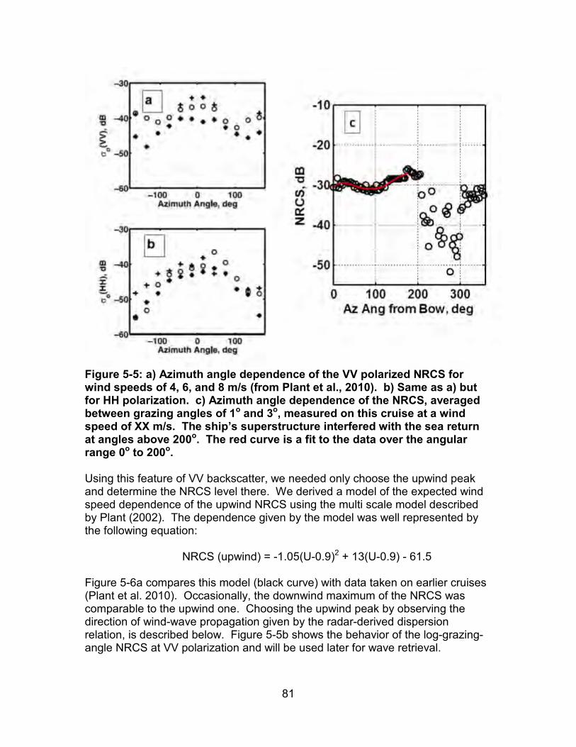
81

Figure 5-5: a) Azimuth angle dependence of the VV polarized NRCS for wind speeds of 4, 6, and 8 m/s (from Plant et al., 2010). b) Same as a) but for HH polarization. c) Azimuth angle dependence of the NRCS, averaged between grazing angles of 1o and 3o, measured on this cruise at a wind speed of XX m/s. The ship’s superstructure interfered with the sea return at angles above 200o. The red curve is a fit to the data over the angular range 0o to 200o. Using this feature of VV backscatter, we needed only choose the upwind peak and determine the NRCS level there. We derived a model of the expected wind speed dependence of the upwind NRCS using the multi scale model described by Plant (2002). The dependence given by the model was well represented by the following equation: NRCS (upwind) = -1.05(U-0.9)2 + 13(U-0.9) - 61.5 Figure 5-6a compares this model (black curve) with data taken on earlier cruises (Plant et al. 2010). Occasionally, the downwind maximum of the NRCS was comparable to the upwind one. Choosing the upwind peak by observing the direction of wind-wave propagation given by the radar-derived dispersion relation, is described below. Figure 5-5b shows the behavior of the log-grazing-angle NRCS at VV polarization and will be used later for wave retrieval.

82

Figure 5-6: a) the model function used here to retrieve wind speeds (black curve) compared with data taken on two earlier cruises in 2005 (asterisks) and 2006 (circles) [Plant et al., 2010]. Data and model are for upwind looks at grazing angles between 1o and 3o. b) Dependence of the normalized radar cross section in dB on grazing angle. Squares show predictions of the multiscale model at wind speeds of 4 (blue), 8 (green), and 12 m/s (red) (Plant, 2002). The curves show σo(θg) used for wave retrieval at the same wind speeds. Figure 5-7 compares wind speed and direction obtained from the radar with those given by the ship’s anemometer on August 13. The rms difference between speeds from the ship’s anemometer and the radar is 2.8 m/s while that between the directions is 18o. This is sufficiently encouraging to believe that a VV polarized radar on a ship can yield viable wind fields around the ship, perhaps with somewhat refined antennas and model function.

83

Figure 5-7: a) Wind speeds from radar (open circles) compared with those from the ship’s anemometer (triangles). b) Wind directions from radar (open circles) compared with those from the ship’s anemometer (triangles). Rms differences in speed and direction are 2.8 m/s and 18o, respectively. 5.6 Current and Doppler Measurements As the antennas rotated, recorded were the spatial dependence of both the cross section and scatterer velocity every three seconds in any particular direction. Two-dimensional spectra of such space-time series are displayed in Figures 5-8a and 8b while the antenna was looking into the wind. The dashed lines in these plots show the first-order dispersion relation ω = �gk + 𝐤 ⋅ 𝐔

00:00 06:00 12:00 18:00 00:000

5

10

15

20

25

30


Win

d S

peed

(m/s

) a

00:00 06:00 12:00 18:00 00:00280

300

320

340

360

380

400

420


Win

d D

irec

tion

(°T)

b

84

where ω is angular frequency, k is wave vector and k is its magnitude, g is gravitational acceleration and U is the current vector. In Figure 5-8, U was set to be the negative of the component of ship velocity along the antenna-look direction. The dispersion relation folds back at the upper and lower Nyquist frequencies of 0.15 Hz. (Note that this is the Nyquist frequency for NRCS and Doppler velocity samples, not for the Doppler spectrum.) Wave energy clearly lies near the first-order dispersion relation but it is aliased due to our 3.3 sec revisit time. Other features that lie off the first-order dispersion relation can also be seen in the spectra. These higher-order features have been identified as being primarily due to breaking waves (Plant and Farquharson, 2012; Plant, 2012).

Figure 5-8: Wavenumber-frequency spectra of space-time images obtained from CORAR when looking into the wind. The top row is original, aliased spectra and the bottom row are dealiased, filtered spectra. The left row is from space-time images of NRCS while the right row is from Doppler velocities. The sampling rate was 3.3 seconds. Consider unwrapping these spectra by translating the bottom half to sit on top of the figure and the top half to lie beneath the bottom of the figure. If these unwrapped spectra are filtered with a wide bandwidth around the nominal first-order dispersion relation, i.e., one that includes only ship motion, and only the branch with the highest level of energy above is kept, the spectrum clearly

85

indicates the direction of wave travel. This is shown in Figures 5-8c and 5-8d. In this case, it is clear that the wind waves propagate toward the radar since the antenna is looking upwind. In some directions, the wave components were very low and neither branch of the dispersion curve clearly contained the most energy. In these cases it was not possible to determine a wave direction, or even the existence of waves, and we assumed that no waves existed in this direction. Assuming that the radar responds only to waves travelling along the direction in which the antenna is looking, the component of current in that direction can be obtained by fitting the dispersion relation to the unwrapped, filtered data taken when waves are clearly evident. This was accomplished by varying the component of U along the antenna-look direction until we obtained the best fit to the maxima of the return power as a function of wavenumber and frequency. If this is done for all look directions and the ship velocity subtracted in each direction, then the current produces a sinusoidal plot versus azimuthal look direction. It is a simple matter to pick the current magnitude and direction. There was no comparison measurement of current magnitude and direction during the cruise. However, a pitot tube was located near the bow of the ship at a depth of about 3 meters pointing in the direction of the ship’s heading. This pitot tube gave a value for the component of current in the heading direction when the ship speed was subtracted. These are compared with current components from the radar in the same direction in Figure 5-9. The agreement is very good. This supports the validity of the radar measurements of current.

Figure 5-9: Time plot of the current in the direction of the ship’s heading as measured by the ship’s pitot tube (triangles) and by the radar (circles).

00:00 06:00 12:00 18:00 00:00-1

-0.5

0

0.5

1


Curr

ent a

long

Hea

ding

(m/s

)

(>0 ==> to ship)

86

Since CORAR is coherent, one might think that the centroid (first moment) of mean Doppler spectra could be used to measure currents in addition to the method relying on the dispersion relation described above. However, these measurements emphatically show that the mean Doppler centroid is not primarily a measure of the current. Figure 5-10 compares the current measured using the dispersion relation with the apparent currents derived from the Doppler centroid. Both measurements were made at 21:00 UTC on August 13. The Doppler centroid yields apparent currents that are much larger than those derived from the dispersion relation. Furthermore, the apparent current obtained when the antenna was looking upwind (up wave) is larger than that obtained when looking downwind. It appears that the correlation between received power and Doppler offset first described by Hasselmann and Schieler (1970) dominates the Doppler centroid in this case. This correlation is evidently higher looking upwind when breaking waves contribute more to both the received power and Doppler velocity than when looking downwind.

Figure 5-10: Comparison of currents measured using the dispersion relation (a) with apparent currents from the Doppler centroid (b). Both sets of measurements were obtained on August 13, 2008 at 21:00 UTC. The wind speed was 16.9 m/s from 341oT. 5.7 Wave Measurements, Phase-resolved and Statistical Having determined the wave propagation direction and the current component in cases when waves were clearly evident in a particular antenna-look direction, we then filtered more tightly around a dispersion relation that included the current and ship velocity. We kept both the filtered spectrum and the filtered Fourier transform (whose magnitude-squared is the spectrum) that resulted from these procedures. Thus, the components of the variations of the NRCS and Doppler

87

velocities that resulted from the action of the linear part of the surface waves were kept; nonlinear effects were discarded. Recall that only variations with wavelengths less than 420 m are included in our analysis. Inverse transforming these quantities produced the spatial and temporal variations of the NRCS and Doppler velocities caused by the first-order surface waves. From these variations in the NRCS and Doppler velocities, one can, in principle, obtain the surface-wave height. For the variations in Doppler velocities, the procedure is straightforward. At each time step, the measured spatial variations in Doppler offset, fd(R, t), in a given direction, indicated by “i” are converted to velocity:

Vi(R, t) = λofdi(R, t)2cosθgo

where R is range, λo is the microwave length, and θgois the mean grazing angle at that range. Then the surface displacement, ηi, is easily obtained in K-space:

ηi(K, t) =Vi(K, t)ωi(K)

The Fourier transform of ηi(K, t) is the desired ηi(R, t). Because the velocity at the wave crest changes signs when the wave travels the opposite direction, we have to set

ηi(R, t) = −sgn(K) ∗ ηi(R, t) where sgn(K) is positive for waves traveling in the range direction and negative in the opposite direction. We let sgn(K) = 0 when waves could not be detected in a given direction. The procedure for transforming temporal-spatial variations in received power into wave amplitude is not so straightforward. We may write the received power, Pr, as follows:

Pr = C σoA

R4 = ⟨Pr⟩ + ⟨Pr⟩ �δPr⟨Pr⟩

� = ⟨Pr⟩ + ⟨Pr⟩�m(K)S(K, t) exp(−iKR) dK

where C is constant, σo is normalized radar cross section, A is the area of a resolution cell, brackets indicate a spatial average, m is the modulation transfer function, S is (large-scale) surface slope, K is the long wave number. For pulsed radars such as CORAR, A is proportional to R/cosθg. Since σo is a function of grazing angle, θg, and the small scale roughness spectrum, ψ, we have

88

δPr⟨Pr⟩

=δσo⟨σo⟩

+δsecθgsecθgo

− 3δR⟨R⟩

= �1⟨σo⟩

∂σo∂θg

|θgo + tanθgo� δθg + 1⟨σo⟩

∂σo∂ψ

|⟨ψ⟩δψ − 3δR⟨R⟩

where θgo is the mean grazing angle at range R. But

δθg = dηdR

= S and

δR⟨R⟩

= ηh

where h is the height of the antenna. Fourier transforming, we may make the following identification:

m(K) = mt + mh(K) + mr(K) where the tilt modulation transfer function (MTF) is

mt = ∂ln⟨σo⟩∂θg

|θgo + tanθgo

the hydrodynamic MTF is

mh(K) = 1⟨σo⟩

∂σo∂ψ

δψS

|⟨ψ⟩

and the range-change MTF is

mr(K) = −3

Kh

Then,

δPr⟨Pr⟩

= �m(K)S(K, t) exp(−iKR) dK

This is the standard view of the MTF when received power is not calibrated into NRCS. By Fourier transforming the spatial variations in Pr, dividing by m(K), and inverse transforming, one obtains S(R,t). However, we relate Pr to σo using mean values of A and R. This means that

δPr⟨Pr⟩

= δσo⟨σo⟩

89

and the tanθgo term is not in mt and mr = 0. Therefore, we have

𝑆(𝑅, 𝑡) =1⟨σo⟩

�δσo(K, t)

m(K) exp(iKR) dK

The above MTF definitions are valid in deep water when the wave travels toward or away from the antenna. The hydrodynamic MTF, which accounts for long-wave-induced variations in small-scale roughness, is poorly characterized but known to be a function at least of microwave frequency, wind speed, wind direction, and K (Keller and Plant, 1990; Plant et al., 1993; Hara and Plant, 1994). Although its value varied somewhat from one data set to another and depended on the value assumed for the relaxation time, Hara and Plant found that mh was always less than 12 in magnitude. On a Bragg/composite surface model, the tilt MTF is between 77 and 230 for grazing angles between 1o and 3o for a pulsed radar like CORAR. Therefore, we shall follow Dankert and Rosenthal (1994) and omit mh in the calculations to follow. We note, however, that this may not be an entirely satisfactory assumption since mh is in phase with the wave amplitude while mt is 90o out of phase. With these assumptions, m(K) = mt is not a function of K so we have:

𝑆𝑖(𝑅, 𝑡) =1

mt⟨σo⟩�δσo(K, t) exp(iKR) dK =

𝛿𝜎𝑜𝑑𝐵(𝑅, 𝑡)𝑚𝑡𝑑𝐵

where 𝛿𝜎𝑜𝑑𝐵(𝑅, 𝑡) is the measured cross section in dB that has been detrended, mtdB is 𝑚𝑡 converted to decibels, or mt

dB = 23 mt. It is most convenient to implement this equation for S by finding the difference in grazing angle, 𝜃𝑔 − 𝜗𝑔𝑜, where the measured 𝛿𝜎𝑜𝑑𝐵(𝑅, 𝑡) is equal to ⟨𝜎𝑜𝑑𝐵�𝜗𝑔�⟩ − ⟨𝜎𝑜𝑑𝐵�𝜗𝑔𝑜�⟩ given by a model function. Then 𝑆𝑖 = tan (𝜃𝑔 − 𝜃𝑔𝑜). Once the slope has been determined, it is straightforward to determine ηi(K,t):

ηi(K, t) = Si(K, t)

jK

where j = √−1. ηi(R,t) is then the Fourier transform of ηi(K,t). No multiplication by sgn(K) is necessary in this case because increased power return always comes from the side of the wave facing the antenna. We still set ηi = 0 in directions where no waves could be detected, however.

90

In practice the determination of the model function ⟨𝜎𝑜𝑑𝐵�𝜗𝑔𝑜� ⟩ was done by attempting to get the best match between waveheights from Doppler shifts and those from the NRCS. The resulting model function, which had to include a dependence on wind speed, was checked against predictions of the multiscale model (Plant, 2002). The results are shown in Figure 5-6b. Note that only the slope of the resulting model function is required to retrieve wave heights. Figure 5-11 shows wave heights in different look directions derived from both the NRCS and Doppler velocities. The figure shows, from top to bottom, wave heights looking upwind, downwind, up swell, and down swell. While wave heights measured by the two different methods are certainly not identical, they are well correlated. Because of our spectral unwrapping procedure, such plots can be produced every 1.1 seconds so that one can easily look at many comparisons. The one shown is fairly representative. We will look into the similarities and differences of the results of the two methods in more detail below.

Figure 5-11: Comparison of wave heights derived from Doppler offsets (red) and received power (black). From the top, the directions of look are upwind, downwind, up swell, and down swell. Data were taken on August 13, 2008 at 17:57 UTC

91

These measurements along the various azimuth angles were used to determine the two-dimensional, phase-resolved surface displacements around the ship. The results obtained above for ηi(R, t) were Fourier transformed to get ηi (K, t). We got the corresponding spectral density of this wave of wavenumber K traveling in the antenna-look direction from the equation

𝐹𝑖(𝐾, 𝑡) =|𝜂𝑖(𝐾, 𝑡)|2

𝐾𝛥𝐾𝛥𝜙𝑡

where the Δφt is the total angular resolution in K-space including antenna beam width, angular rotation during data collection and the azimuthal length of the resolution cell. This total angular resolution is given by (Plant et al., 1987):

Δφt = 4√ln2 ⟨2

(KRφh)2 +φn2

2⟩

where

φn = �φp2 + (ΩTn)2

and

φp = φh

cosθg√2ln2

The brackets indicate an average over range, Ω is the antenna rotation rate in rad/sec and φh is the one-way, half-power, full antenna horizontal beamwidth. All angles are in radians. Our two major assumptions are that the radar responds only to waves travelling along the radar’s line of sight and that the Fourier components ηi(K,t) are valid everywhere in the vicinity of the ship. With these assumptions, we can obtain the two-dimensional wave field around the ship as follows:

η(x, y, t) = �√2i

Ai(K, t)cos (sgn(𝐊 ⋅ 𝐑)(K(x sin αi + y cos αi) + φ1) − ωit)

where x and y are coordinates in the east and north directions, αi is the compass angle of the ith look direction, and ωi is the angular frequency in the ith direction determined from the measured dispersion relation. The sign of the cosine of the angle between the antenna look direction and the direction of wave travel is indicated by sgn(𝐊 ⋅ 𝐑). Also,

Ai(K, t) = �Fi(K, t)KΔKΔϕ/Δϕt

92

which is simply ||η(K, t)|�𝛥𝜙/𝛥𝜙𝑡. The phase of η(K,t) is 𝜑1 for the initial look in each direction. An example of phase-resolved waves around the ship obtained by this procedure using 3.3 seconds of data (one interleaved rotation) is given in Figure 5-12. Again, the waves from the two methods are highly correlated but not precisely the same. Because of de-aliasing, images can be produced such as those shown in Figure 5-12 every 1.1 seconds. Thus one can compare the time series of surface displacements from a spatial bin near the buoy with the time series of surface displacements from the buoy. Both the buoy and CORAR received a GPS signal so that time and location of CORAR and the buoy could be determined very accurately. The difference in the location of the buoy and the ship were tracked during the time of data collection and corrected for changes., resulting in the fact that the change in separation was never more than one range cell in either the east or north direction. The buoy was located approximately at coordinates (60,-460) m in Figure 5-12. A comparison of various time series after location had been corrected is shown in Figure 5-13. Clearly the agreement between the various time series is not perfect but the correlations are sufficiently high to encourage development of this technique.

Figure 5-12: Phase-resolved waves around the R/V Thompson obtained from CORAR’s received power (left) and Doppler offsets (right). Data were taken on August 13, 2008 at 17:56 UTC.

93

Once the spectral densities of the waves in different look directions have been calculated, it is a simple matter to obtain the rms wave height by integration followed by temporal averaging. This was done for a set of files taken 15 minutes apart. The averaging time was 54 seconds. Figure 5-14 shows the significant wave heights, Hs, obtained by multiplying these rms heights by 4 for 72 samples from August 13. The circles are from the NRCS, the asterisks are from the Doppler velocities, and the X’s are from the buoys that were deployed on that day. A general trend of increasing Hs as the duration of wind speeds between 15 and 20 m/s increased is seen in the figure. However a significant decrease in wind speed and an accompanying small shift in wind direction occurred at about 8:00 UTC. A corresponding small dip in the significant wave height is observed at about this time.

Figure 5-13: Comparison of various time series from CORAR and the buoy located at (60,-460) m in Figure 12 on August 13, 2012. a) Comparison of buoy wave heights (black) and those from Doppler shifts (red). b) Comparison of buoy wave heights and those from cross sections (green). c) Comparison of wave heights from Doppler shifts (red) and from cross sections (green).

23:42:00 23:42:30 23:43:00 23:43:30 23:44:00-202

Buoy(black), Doppler(red), NRCS(green)

a

23:42:00 23:42:30 23:43:00 23:43:30 23:44:00-202

Surf

ace

Dis

plac

emen

t, m

b

23:42:00 23:42:30 23:43:00 23:43:30 23:44:00-202

Time on August 13, 2008

c

94

Figure 5-14: Significant wave heights, Hs, obtained from the phase-resolved wave fields measured by CORAR around the R/V Thompson on August 13. Asterisks show Hs from Doppler velocities, circles show Hs from the NRCS, and the X’s show Hs measured by buoys that were tethered to the ship. By plotting spectral densities in all look directions on a polar plot, averaging over all spectra obtained in our 162 second time record, and smoothing the resulting spectrum over four bins in range and azimuth, we produced the directional wave spectra shown in Figure 5-15a and 5-15b. The components of the spectra moving toward the radar and doubled those moving away have been omitted. Thus, the spectra indicate the direction toward which the waves travel. The black lines in these panels give the wind direction; from the center out is the direction toward which the wind blows. By further integrating over azimuth angles the omni-directional spectra shown in Figures 5-15c and 5-15d resulted. These spectra are defined by:

F(K) = �⟨Fi(K, t)⟩i

Δϕ

When multiplied by K and integrated over K, they yield the mean-square wave height. Four times the square root of this value is Hs given in the upper right corner of each plot as is Hs from the buoy. The red curves in the lower panels show omni-directional spectra from the buoy. Note that in converting these buoy spectra from frequency to wave number, the magnitude and direction of the current had to be known very accurately.

00:00 06:00 12:00 18:00 00:000

1

2

3

4

5

6


Sign

ifica

nt W

ave

Hei

ght (

m)

95

Figure 5-15: a) Directional wave spectra from cross sections. b) Directional wave spectra from Doppler shifts. c) Omni directional wave spectra from cross sections (black) and from the buoy (red). d) Omni directional wave spectra from Doppler shifts (black) and from the buoy (red). The black line in the upper panels show the direction toward which the wind blows, from the center out. Significant wave heights, Hs, are shown in the upper right corner of the lower panels. Data were taken on August 13, 2008 at 17:55 UTC. Researchers expect F(K) to depend on K approximately as K-4 at high wavenumbers so that the curvature variance spectrum in the wind direction, K4Fi(K), has a value between 0.001 and 0.002 for wavenumbers near 0.3 rad/m. This is usually called “α” since it is the same as the coefficient of the frequency spectrum first proposed by Phillips (1958). We attempted to determine the value of α from our spectra by using the multi-scale model of Plant (1990) but adjusting the value of α to match our spectra at high wavenumbers. Figure 5-16 shows this fitting procedure and the values of α obtained. Figure 5-16a shows both wave height variance spectra (upper curves) and curvature variance spectra (lower curves). Solid curves are from Doppler velocities while dashed curves are from the NRCS. The vertical dotted line shows the wavenumber at which the radar-derived spectra were matched to spectra from the multi-scale model. The figure shows that spectra from the NRCS are higher at low frequencies and lower at high frequencies than spectra from Doppler velocities. The K-4 spectrum also appears to provide a better fit to the high-wavenumber spectra from the Doppler velocities.

96

Figure 5-16: a) Wave height variance spectra integrated over azimuth (upper curves) and curvature variance spectra integrated over azimuth angle (lower curves). Solid curves are from Doppler and dashed curves are from cross section. Vertical dotted line shows the wave number at which radar spectra and theoretical spectra were matched. b) 1000 times Phillips’ α versus wind speed. Circles are from Doppler, triangles are from cross section, and the line shows Banner’s relation 𝜶 = 𝟎.𝟎𝟎𝟏𝟖 �𝑼/𝒄𝒑. c) Ship speed (solid curve) and α from Doppler offsets. Note the high α values when the ship speed was high.

97

Figure 5-16 b shows the values of α necessary to produce the fits shown in Figure 5-16a along with the values obtained from Banner’s form, which may be written

α = 0.0018 �U/cp

where U is wind speed and cp is the speed of the wave at the peak of the wave-number spectrum derived from the radar-measured spectra (Banner, 1990). There are seven circles above α = 3 shown in Figure 5-16b. As Figure 5-16c shows, these all come from files where the ship speed was high. The reason for this is unknown but without these high values, the average α from Doppler shifts is 0.0015 while that from the cross sections is 0.0006. The mean of Banner’s value of α over the range of wind speeds shown in Figure 5-16b is 0.0018. It appears that spectra from Doppler velocities yield better levels of the high-wave number spectrum than those from the NRCS. 5.8 Conclusions This work has shown that winds, waves, and currents can all be measured by a coherent shipboard radar operating at vertical polarization and low-grazing angles. Currents were probably the most accurate of the quantities measured by the radar. These were determined by fitting the first-order surface wave dispersion relation to measurements along a series of azimuth angles by varying the current component along each azimuth angle. The resulting currents tracked current components measured by the shipboard pitot tube to within a few cm/s. The work showed that these currents could not explain the frequencies of the centroids of the Doppler spectra measured by the coherent radar. These centroids were at frequencies that implied much larger velocities as their cause, and velocities that were larger looking upwind than downwind. These results show that these large Doppler offsets are a manifestation of the correlation between wave-induced backscattered power and wave-induced Doppler shifts, as first described by Hasselmann and Schieler (1970), probably augmented by breaking wave effects. Raster scans of Doppler spectra from a CW microwave system illuminating a small spot on the sea surface clearly illustrate this effect (Keller et al., 1986). Winds measured around the ship by the radar tracked those measured by the ship’s anemometer with rms accuracies reminiscent of early satellite scatterometer winds. The rms difference in speed was 2.8 m/s and that in direction was 18o. While these are not as small as one might wish, indications are that the use of antennas with somewhat wider vertical beamwidths could improve the numbers. Transmitting more power should also help.

98

Finally, this work showed that both phase-resolved wave fields and the statistical properties of these fields could be measured within an area approximately 2.2 km on a side using both measured Doppler shifts and measured cross sections. These agreed, again, reasonably well with similar quantities measured at a single point by a buoy. The primary assumptions used to compute these wave fields from the radar return were that the radar responded only to waves travelling very close to its look direction, that measured Fourier components were valid everywhere around the ship, and that the wave-induced variations in NRCS were primarily due to local changes in grazing angle. For the longer waves, the unidirectional assumption may break down, although it appeared to be accurate at least up to the 100 m waves encountered in our experiments. In general, wave spectra from Doppler shifts seemed to fit buoy spectra better than did wave spectra from cross sections, being better fits at both low and high wave numbers. Interestingly, however, phase-resolved surface displacements from cross sections were somewhat more correlated with those measured by the buoy than were surface displacements from Doppler shifts. However, it is well known that the MTF is large at low wave numbers and low at high wave numbers. Therefore, the higher correlations for wave heights from the NRCS could simply be due to this effective smoothing by the MTF since it has not been removed in this work. The technique used in this work is quite different from the technique often used to retrieve phase-resolved wave heights from marine radar images. These often use data from only small rectangles in the radar image, obtaining spectra through Fourier transforms and wave heights via a modulation transfer function. These techniques can respond only weakly to waves travelling perpendicular to the mean look direction of the rectangle for three reasons. First of all, phenomena that produce wave-induced variations of the received power and radial velocity are much weaker for waves travelling perpendicular to the antenna look direction. Second, even though a marine radar has a very narrow beam width, it is not infinitely narrow so it produces some K-space angular discrimination against waves travelling perpendicular to the look direction. Finally, all these techniques filter around the dispersion relation, which rather efficiently discriminates against waves travelling perpendicular to the look direction. For these reasons, a technique which utilized data from only a small part of the radar image cannot capture waves travelling perpendicular to the mean antenna-look direction of this part. Since mixed seas are the rule rather than the exception on the ocean, this technique cannot produce correct wave heights most of the time. While none of the radar measurements reported here agreed perfectly with those from the more standard instruments, the agreement was sufficiently promising to encourage continued development of the radar techniques. The research team is in the process of making improvements to the radar that will lead to winds, waves and currents that more closely agree with in situ measurements.

99

5.9 References Banner, M.L., Equilibrium spectra of wind waves, J. Phys. Ocean., 20, 966-984,

1990. Chang, M-H, R-C Lien, Y.J. Yang, T.Y. Tang, and J. Wang, A Composite View of

Surface Signatures and Interior Properties of Nonlinear Internal Waves: Observations and Applications, J. Atmos. Ocean. Tech., 25, 1218 – 1227, DOI: 10.1175/2007JTECHO574.1, 2008.

Dankert, H., J. Horstmann, and W. Rosenthal, Wind- and Wave – Field

Measurements Using Marine X-Band Radar-Image Sequences, J. Ocean. Eng., 30(3), 10.1109/JOE.2005.857524, 534– 542, 2005.

Dankert, H., and W. Rosenthal, Ocean surface determination from X-band radar-

image sequences, J. Geophys. Res., 109, C04016, doi:10.1029/2003JC002130, 2004.

Hara, T. and W.J. Plant, Hydrodynamic modulation of short wind-wave spectra

by long waves and its measurement using microwave backscatter, J. Geophys. Res., 99 (C5), p. 9767-9784, 1994.

Hasselmann, K., and M. Schieler, Radar backscatter from the sea surface,

Eighth Symp. On Naval Hydro., Rome, Italy, 361-388, 1970. Jones, W.L., L. C. Schroeder, and J. L. Mitchell, “Aircraft measurements of the

microwave scattering signature of the ocean,” J. Oceanic Eng., vol. OE-2, pp. 52-61, 1977.

Keller, W.C., W.J. Plant, and G.R. Valenzuela, Observations of breaking ocean

waves with coherent microwave radar, in Wave Dynamics and Radio Probing of the Ocean Surface, ed. O.M. Phillips and K. Hasselmann, Plenum Publishing Corp., 285-293, 1986.

Keller, W.C., and W.J. Plant, Cross sections and modulation transfer functions at

L- and Ku-Bands measured during the TOWARD experiment. J. Geophys. Res., 95 (C9), 16,277-16,289, 1990.

Nieto Borge, J.C., G.R. Rodriquez, K. Hessner, and P. I. Gonzalez, Inversion of

Marine Radar Images for Surface Wave Analysis, J. Atmos. Ocean. Tech., 21, 1291-1300, 2004.

Phillips, O.M., The equilibrium range in the spectrum of wind-generated ocean

waves, J. Fluid Mech., 4, 426-434, 1958.

100

Plant, W.J., W.C. Keller, A. Cross, Parametric dependence of ocean wave-radar modulation transfer functions. J. Geophys. Res., 88(C14), 9747-9756, 1983.

Plant, W.J., W.C. Keller, A.B. Reeves, E. Uliana, and J.W. Johnson, Airborne

microwave Doppler measurement of ocean wave directional spectra, Intl. J. Remote Sensing, 8 (C3), 315-300, 1987.

Plant, W. J., W. C. Keller, V. Hesany, and K. Hayes, Measurements of the

marine boundary layer from an airship, J. Atmos. Oceanic Technol., 15, 1433–1458, 1998.

Plant, W.J., A stochastic, multiscale model of microwave backscatter from the

ocean, J. Geophys. Res.,107(C9), 3120, doi:10.1029/2001JC000909, 2002.

Plant, W. J., W. C. Keller, K. Hayes, and G. Chatham, Normalized radar cross

section of the sea for backscatter: 1. Mean levels, J. Geophys. Res., 115, C09032, doi:10.1029/2009JC006078, 2010.

Plant, W.J. and G. Farquharson, Origins of features in wavenumber-frequency

spectra of space-time images of the ocean, J. Geophys. Res., 117, C06015, doi:10.1029/2012JC007986, 2012.

Plant, W.J., Whitecaps in deep water, Geophys. Res. Ltrs., 39, L16601,

doi:10.1029/2012GL052732, 2012.

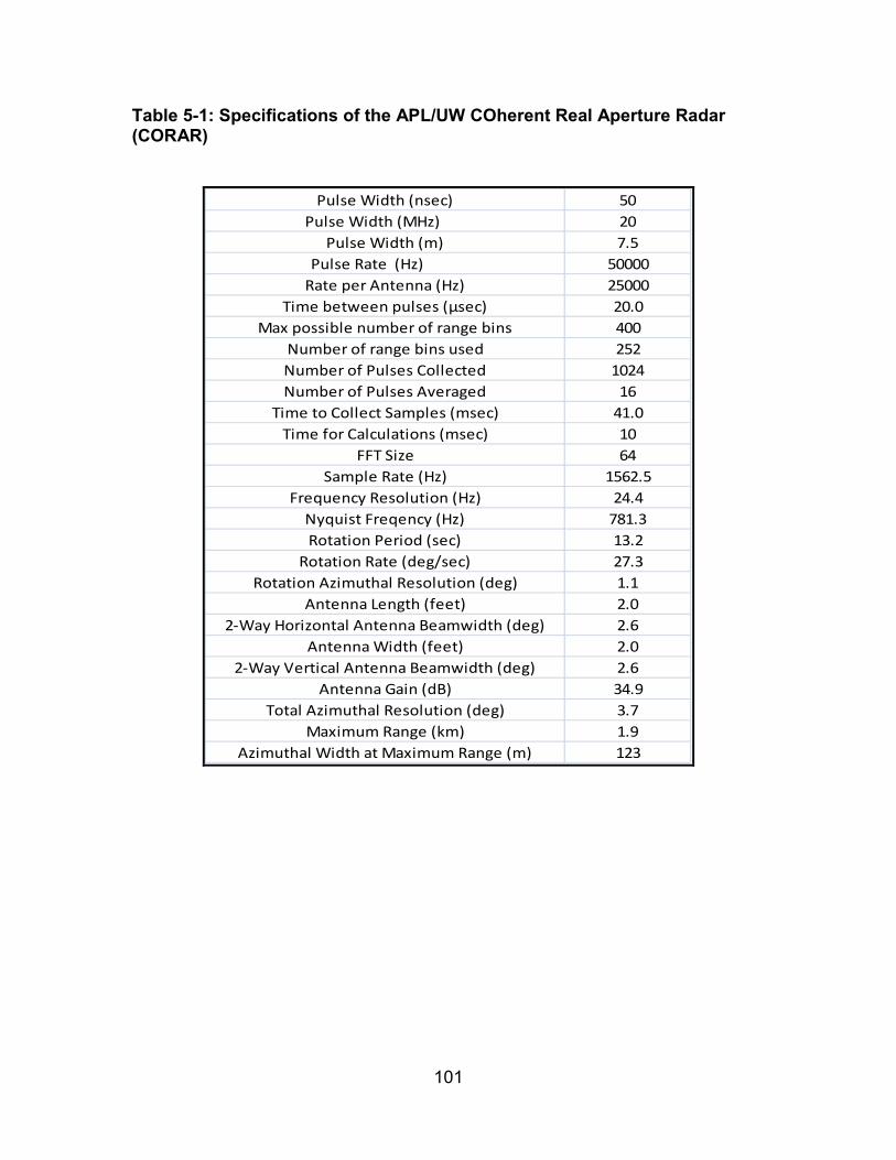
101

Table 5-1: Specifications of the APL/UW COherent Real Aperture Radar (CORAR)

Pulse Width (nsec) 50Pulse Width (MHz) 20

Pulse Width (m) 7.5Pulse Rate (Hz) 50000

Rate per Antenna (Hz) 25000Time between pulses (μsec) 20.0

Max possible number of range bins 400Number of range bins used 252Number of Pulses Collected 1024Number of Pulses Averaged 16

Time to Collect Samples (msec) 41.0Time for Calculations (msec) 10

FFT Size 64Sample Rate (Hz) 1562.5

Frequency Resolution (Hz) 24.4Nyquist Freqency (Hz) 781.3Rotation Period (sec) 13.2

Rotation Rate (deg/sec) 27.3Rotation Azimuthal Resolution (deg) 1.1

Antenna Length (feet) 2.02-Way Horizontal Antenna Beamwidth (deg) 2.6

Antenna Width (feet) 2.02-Way Vertical Antenna Beamwidth (deg) 2.6

Antenna Gain (dB) 34.9Total Azimuthal Resolution (deg) 3.7

Maximum Range (km) 1.9Azimuthal Width at Maximum Range (m) 123

102

6 MAPPING CURRENTS AND WAVES USING DOPPLER SONAR

Principle Investigator: Jerry Mullison, Teledyne RD Instruments 6.1 Technical Summary The Horizontal ADCP measurement has the inherent information necessary to estimate waves on short timescales using spatial domain processing. Further analysis will shed more light on best approaches and operational bounds. Directional waves are possible using the approach though longer profiling range may be important to resolving phase of long period waves spatially. The method seems well suited to creating a real-time wave predictor. There are likely to be limitations when the sea state is exceptionally broadband or very small. 6.2 Turbulence Measurement Approaches A conventional bottom-mounted geometry with four upward-looking beams in Janus configuration mounted at 45 degrees azimuth to the flow direction is currently the best approach to measuring vertical profiles of conventional turbulent parameters such as outer length and velocity scales and dissipation rate, whether in pre-deployment site selection studies or upstream monitoring of existing systems. In high-current sites, considerable care is needed to ensure that the instrument stays fixed to the bottom. Supplementing a bottom-mounted ADCP with a downward-looking ADCP mounted on a buoy containing inertial sensors to remove buoy motion would confirm that the profiles measured by the upward-looking system are not being biased by the linear increase in measurement cell separation with height. For highly-instrumented research sites, it may be useful to supplement upstream ADCPs with single-beam Doppler sonars at a small number of depths mounted on the turbine structure and pointed upstream. These could be separate but synchronized ADCPs, one beam of each pointing upstream and the others pointed upward and to the sides. 6.3 Mixed Sea State Anyone who has spent time looking at arriving waves in a mixed up, broadband sea state, knows that the higher frequency waves sometimes add up to form a peak, but this peak seldom lasts as the waves move apart. A surfer will look for coherent structure in the approaching waves when the sea state is mixed, because the longer period coherent waves are more likely to be significant in shallower water, and their propagation can be predicted amidst the background.

103

Our expectation based on this data, is that the approach will low pass filter the output. It will favor the bigger, longer, more coherent waves and produce a non-result for all else. In the context of trying to produce a wave predictor, or early warning system we would most likely be addressing the biggest, longest period waves. This is a benign characteristic under many circumstances. In a mixed sea state it will likely show mostly the largest longest periods because the spatial domain approach is using sub-surface horizontal orbital velocity, it selectively favors bigger, longer period waves. Because the approach will not estimate wave number for frequencies that are not coherent over the span of the array it also favors coherent waves of any size. 6.4 Groups Another condition that one might like to address is wave groups. If for example, the purpose was to use the system as a wave predictor in order to protect turbines used for renewable energy, then wave groups become important. Due to the dispersion relationship waves that have propagated for some time tend to form groups. If the sea is rough then equipment can be protected. If the sea is calm then the equipment can be optimized for energy efficiency. If there are wave groups however, the sea may be calm, then sporadically a set of structurally significant waves will arrive in a group. In this case one might like to see the group coming and adapt to protect, then turn efficiency back up until the next group arrives. The spatial domain approach could provide the kind of short time scale warning of an approaching group that would allow real-time adaptation.

6.5 Background The development of offshore renewable energy sources (wind, wave and in-stream) requires knowledge of the statistics of oceanic waves and currents for site selection and, in the case of wave and current extraction devices, ongoing monitoring for optimization of the efficiency of the device. This section of the report focuses on the utility of Doppler sonar for these applications, and differentiates between traditional Acoustic Doppler Current Profilers (ADCPs) oriented vertically for high resolution current profiles through the water column and ADCPs oriented horizontally to provide large spatial coverage with high resolution within a single horizontal layer. ADCPs of various types are in widespread use throughout the world, providing measurements of currents, waves and turbulence parameters to researchers and

104

operational decision makers. TRDI ADCPs traditionally vertically project four beams in orthogonal pairs (see the various depiction deployed instruments in Figure 6-1), and measure the component of the fluid velocity along each beam which allows measurement of several parameters of critical interest in siting and monitoring of renewable energy devices. First, assuming the mean velocity is homogeneous over the horizontal span of the beams (generally a good assumption in the mean), the current can be recovered by differencing opposing beams. Second, since the second order statistics of the wave field are also horizontally homogeneous, the frequency-direction spectrum of the waves can be recovered by a bottom-mounted, upward-looking ADCP in moderate water depths (typically less than 20 m). And third, a great deal of work has been accomplished from ADCPs with four and five beams to measure turbulence parameters such as Reynolds stresses and Turbulent Kinetic Energy. That is, a single ADCP can be used to gather measurements of currents, waves and turbulence parameters: three parameters that are of critical interest in site selection and monitoring for renewable energy devices.

Of particular interest to the renewable energy community is the potential to forecast the waves a few seconds into the future. This is because the energy in a typical wave field can rapidly change over several orders of magnitude, and it would be useful to have some short term indicator of a pending large event to

Figure 6-1: Illustration of vertically and horizontally oriented ADCPs.

105

allow energy shunting to protect the devices from large events. For turbulence the outer scale turbulence seems far more important than the inertial scale, however there seems to be considerable uncertainty as to which turbulent parameters will eventually prove to have the most utility. Therefore, the results from short term wave forecasting are the primary focus of this report.

6.5.1 Spatial Domain Processing for Horizontal ADCP Waves At any given moment in time, there are a number of different waves (wave frequencies) at a single location. Typically waves are sampled in time from a single stationary location. Often the time series are converted to the frequency domain (power spectra) because each wave frequency can be addressed independently (linear wave theory). This statistical measure of waves usually takes from 10 to 40 minutes. It would however, be valuable to be able to estimate the wave field in the immediate vicinity, at a single moment in time. Clearly the time domain approach does not work at a single instant. The 300 kHz horizontal ADCP (HADCP) presents us with the opportunity to look forward spatially into the wave field to see advancing waves at an instant. The spatial domain approach involves doing FFTs spatially along the beams of the HADCP at a snapshot in time, and creating a wave-number spectrum.

6.5.2 Traditional Time Domain Horizontal ADCP Deployment The HADCP is a horizontally mounted 3 beam, 300 kHz ADCP, with 2 beams at 20 degrees Janus and one beam in the center. The ceramics are large to create a narrow beam and increase range. The application is to measure both near surface currents and wave directional spectra from the unit. The importance of this configuration to Ports, to offshore industry, and renewable energy is that near surface currents and waves can be measured, oncoming, at substantial range from the instrument. The ADCP can be mounted where it is safely out of the way of operations, and directed away from the platform to provide waves and currents information from regions uninfluenced by the presence of boundaries. A 2 Hz sample rate is possible even at long range. In the typical installation, directional waves are determined using phase coherent array processing applied to velocity time series measurements in the virtual array of ADCP range cells (Figure 6-2). 6.6 Deployment Details This analysis was carried out on an historical deployment that was known to have provided high quality currents and wave data using our more traditional time domain analysis and to have compared well with nearby wave buoys. Details of the deployment and conclusions are:

106

Figure 6-2: Horizontal ADCP array geometry (Top View).

• 30 m water depth, 12 m submergence, decent size sea state • Wave direction was from 122 degrees geographic. -25 degree offset from

beam 3 center = 335 degrees relative to beam 3 (the center beam in Figure 6-1).

• 135 m profile range with 4 m bins • 135 m wavelength at the peak period • Spatial aperture limited

6.7 Raw Data Figure 6-3 shows the along beam component of the wave orbital velocity for successive 0.5 second snap shots. One can see that the full wavelength of 135m is just about the same as the range of the along beam profile. The implication is that this deployment setup is spatial aperture limited. While sampling was adequate to avoid the Nyquist limit, the ability to resolve the exact phase of the wave along each beam is limited by the fact that we have not quite sampled a single full wave.

107

Figure 6-3: Sequential along beam profiles of wave orbital velocity show the advancing wave.

Figure 6-4: A single along beam profile is zero filled to create a larger sample space. One of the first challenges to overcome is the mathematical logistics of not having very many samples spatially along each beam. In this setup, we had 35 bins of 4 meters. To improve the resolution of the FFT a longer (128 samples) FFT was performed, and the remainder of the series are zero filled. The resulting wave number spectrum has improved resolution around the peak. To get a frequency domain power spectrum we can assume that the dispersion relationship for gravity waves holds true. In doing this, one simply remaps the x axis to units of frequency rather than units of wavelength. The dispersion relationship is:

𝜔2 = 𝑔𝑘 𝑡𝑎𝑛ℎ(𝑘ℎ) ω is the radian frequency, g is acceleration due to gravity, k is wave number, and h is the bottom to surface water depth.

108

6.7.1 Spatial Domain Results The first thing observed in Figure 6-5 is that the peaks don’t line up and they have different magnitudes. This is reasonable to expect because the arriving waves have a particular direction and the projection of those waves down each beam should scale wave number and magnitude by the cosine of the angle offset to each beam. (Cos(α)2 for power spectra) Because the along beam spectra show that peak magnitude and wave numbers are influenced by wave direction it is reasonable that one might be able to calculate the wave direction by measuring the shift of the peak for each beam and assuming that the wave state around the peak is moderately coherent. Likewise, if one assumes that they are measuring in all three beams, at any moment in time is predominantly a single wave (at the peak), then one can compare the peak magnitudes of each beam to get an estimate of wave direction. Additionally, the range cell spacing (ΔS) along the middle beam is different from the other two beams. The convention for this instrument was to have the range cells equal in perpendicular range from the instrument (along beam 3 axis). They are not equal in size, beam radial, along the beams. This must be accounted for prior to doing any phase shift analysis to determine wave direction.

Figure 6-5: Wave spectrum along each of the three beams.

109

Figure 6-6: Spatially determined peaks line up when wavenumber is corrected for a priori wave direction. In Figure 6- 6 one can see that if the known wave direction is applied to determining the true wavelength from the observed wavelength along each beam, the peaks appear to line up. This does not guarantee a unique solution, however, it is consistent with our expectation of this simple geometrical approach.

Figure 6-7: Wave magnitudes match better when corrected for a priori wave direction. Similarly if one scales the magnitude of the peak based on wave direction (Figure 6-7), then one can find that the peak magnitudes also match better. It is possible that if the sea state is substantially broadband or high frequency then the ability to look for spatially coherent features across all of the beams, at a single moment in time, may be compromised. One can also observe that spreading occurs with the beam at the greatest angle offset to the waves, leading to speculation that this is possibly due to the small array aperture relative to observed wavelength.

110

The resolution around the peak is poor. If one were to estimate wave direction at the peak by measuring the peak magnitude and the peak shift, one would like to have better resolution. Extending the time series with zero fill even further and taking larger FFTs one can reduce quantization error on the peak. Figures 6-8 and 6-9 show 512 sample FFTs for the same data.

Figure 6-8: Longer FFT improves resolution around the peak.

• Because the proposed approach utilizes the magnitude and location of the peak, improved resolution on the peak is desirable.

• Increasing the FFT length to 512 samples resolves the peak better but

generally spreads or smears the wave number spectrum. This is because the sampling range and resolution of the FFT has been artificially increased, but has not actually added any new information beyond the original 35 range cells for each beam.

Figure 6-9: Higher resolution data that is corrected for wave direction in both peak shift and magnitude.

6.7.2 A Simple Approach for Estimating Wave Direction Looking at Figure 6-8 it appears encouraging that one could estimate wave direction at the peak by looking for coherent features to be consistent across all three beams. The result show that one can take a known wave direction and by

111

applying simple geometry get the measured wave number spectra to match with peak position and height. Instead the researcher propose that one could search all valid wave directions, calculate observed wave number for each direction candidate, and look for a best fit across the beams between measured wave number peak and predicted wave number peak. This best fit approach was implemented for both peak wave number shift and magnitude.

6.7.3 Steps Investigated

• Peak magnitude and peak shift are used. • Wave direction determined by searching for a best fit to wave magnitude,

and wave number.

o Model the expected observed wave number if waves are coming from a particular direction.

o Determine measured wave number at the peak for each beam. o Search wave direction looking for minimum square error in wave

number. o Search also works by minimizing error in magnitude. o Approach assumes all of the beams are seeing the same wave

magnitude and wave number in the earth reference frame. In other words the approach assumes the waves are relatively coherent over the array.

In order to evaluate the approach, this team chose to first compare this independent spatial measure of wave direction to their accepted statistical methods that use the time domain. A way of comparing single instants in time with the statistical answer estimated from 17 minutes of data was needed. They chose to calculate spatial domain estimates of wave direction based on averaged power spectra, then accumulating a histogram of these estimates that spanned the entire 17 minutes. Figures 6-10a-d show histograms of directional estimates derived from peak shift matching (red) and peak magnitude matching (blue). As progressively more averaging was used, the variance reduced and the estimate converged to the peak direction estimated by time domain analysis.

112

a) Histogram of directions based on single ping snap shots. 17 minutes of 2Hz samples.

b) Histogram as above but power spectra averaged by 8

c) Histogram as above but power spectra averaged by 64

d) Histogram as above but power spectra averaged by 256 Figure 6-10: Histograms of directions based upon single ping snap shots and different power spectra averaging. An average of all 2048 samples produces a correct direction identical to the time domain approach (335 degrees offset from beam 3). Clearly, there is significant variance in the single sample estimates. A Gaussian fit to the distribution might improve the peak estimate when the number of samples is small.

113

Looking at the width of the directional distribution in the histograms of wave direction in figures 6-10a-d, it was observed that there is not much change in the width with pre-averaging. The distribution appears to be about +- 20 degrees around the statistical peak. While it is unclear exactly how much of this directional width is true environment vs. measurement, the fact that the width does not change much with averaging implies that at least a part of the width observed is true environment. It is clear from the time domain statistics that the directional distribution is of similar width to the spatial domain and that the sea state is a stormy 4-6 m event.

6.7.4 The Value of Knowing Wave Direction There are at least two important reasons for wanting to know the wave direction. Unlike sampling time series from a single location, these researchers are attempting to measure the waves spatially along the beams at an instant in time. As such we do not directly have a measure of frequency or wave period. While one can use the dispersion relationship to connect the dots between frequency and wave number one must first have a way to unambiguously determine the wave number in the direction of propagation.

1. In order to know the wave number in the direction of propagation we must simultaneously find a wave direction that is self consistent with the wave number spectra that are observed along all three beams. Wave direction is important mostly because it is necessary to resolving the wave number (k) in the earth reference frame.

2. Once the wave number k is known, then we can use the dispersion

relationship to determine frequency f. This allows one to calculate the phase speed and therefore the rate at which wave crests will be approaching.

6.8 Looking for Frequency/Phase Rate of Change Another aspect that was evaluated was the ability to measure the changing phase of the waves in real time. The along beam spectra contain phase information. The researchers attempted to measure the phase rate of change from one sample to the next. This estimate of frequency should agree with their calculation of frequency based on the wave number spectrum and the dispersion relationship. Ideally, plotting the two measures of frequency against each other should give a diagonal line of slope 1.0 from corner to corner. Instead, figure 6-11 shows an odd shape. The peak frequency (about 0.1Hz) seems to have good agreement for all of the beams and a 1:1 ratio. Outside of this range the values are not 1:1 or consistent across the beams. It is not expected that this test will be

114

valid for frequencies that had no measurable power or for frequencies that are not coherent across the array. Their assumption that there is a single dominant, coherent wave is not necessarily the case.

Figure 6-11: Frequency determined by averaging phase rate of change from one snapshot to the next.

Figure 6-12: Estimate of frequency using sample to sample phase rate of change, shows best 1:1 correspondence with frequency derived from dispersion relationship, at the peak of power. Figure 6-12 shows that the frequencies that can be most accurately estimated using this technique are also the longest period and have significant measurable power. Intuitively this makes sense. One can expect that small waves and higher frequencies will not be coherent over the array. One can also expect that frequencies that have no wave energy will not be coherent either.

Peak power and longer period also show best estimate of

1:1

115

6.9 Looking for Approaching Waves in Time Another useful way to represent the HADCP data was to simply search for peaks using zero crossing analysis. This approach shows the waves approaching relatively directly (See Figure 6-13). Briefly, a wave arrival countdown was investigated.

Figure 6-13: Horizontal orbital velocity data along the beams.

• The along beam orbital velocity data can be used to create a map of the wave peaks using basic zero crossing methods.

• Once the peaks have been identified, one can use the spatial separation

of our samples along the beam to determine the range to the peaks. 𝑟𝑎𝑛𝑔𝑒 = (𝑏𝑖𝑛# 𝑎𝑡 𝑝𝑒𝑎𝑘) ∗ 𝑏𝑖𝑛 𝑠𝑖𝑧𝑒 + 𝑏𝑙𝑎𝑛𝑘.

• Using the best fit approach detailed above, estimates for direction and

wavenumber k (in the direction of propagation) can be made.

• Calculate frequency using dispersion relationship. 𝑓 = �𝐺 ∗ 𝑘 ∗ tanh (𝑘ℎ)

• 𝐴𝑟𝑟𝑖𝑣𝑎𝑙𝑇𝑖𝑚𝑒(𝑠) = 𝑟𝑎𝑛𝑔𝑒 ∗ 𝑘/𝑓 In Figure 6-14 the wave crests and their relative range along the beams are directly used to create a countdown to arrival.

116

Figure 6-14: Wave crest arrival count down. More than one wave crest is in the range of the instrument (red is further away). 6.10 Turbulence In conversations with researchers working on turbine development, the outer scale turbulence seems far more important than the inertial scale. However, there seems to be considerable uncertainty as to what turbulent parameters will eventually prove to have the most utility, resulting in an expressed desire for comprehensive velocity field measurements with high spatial and temporal resolution considerably beyond the constraints of practicality. A specific concern is characterization of coherent structures and the ability to synchronously link such observations to measurement time series of turbine blade loading and power transients. This concern may stem from analogous problems with wind turbines from Kelvin-Helmholtz breaking-wave structures interacting with turbine blades under moderately-stratified atmospheric conditions and causing unexpectedly high stresses that can shorten the working life of the blades significantly. Although most sites being considered for water turbine installations do not have comparable degrees of stratification, there is still research concern with identifying other coherent structures that could cause analogous problems, such as two-dimensional eddies shed from upstream islands, bathymetric features, or other upstream turbines. The required spatial resolution for identifying relevant coherent structures might be on the order of the blade width or somewhat larger, and definitely a small fraction of the blade length. The required temporal resolution can be calculated from the spatial resolution by scaling with the reciprocal of the mean velocity. Turbulence studies can also be characterized by their place in the life cycle of pre-installation monitoring of potential sites, highly-instrumented monitoring of installations at research sites, and finally routine minimally-instrumented monitoring at ordinary turbine installations. Although the instrumentation needs vary considerably over this life cycle, there is a consistent need for monitoring of upstream turbulence and mean flow conditions at sufficient distance from the turbine (if present) to be out of its range of significant hydrodynamic influence.

0

2

4

6

8

10

12

14

1 12 23 34 45 56 67 78 89 100

111

122

133

144

155

166

177

188

199

210

221

232

243

254

265

276

287

298

309

320

331

342

353

364

375

386

397

408

419

430

441

452

463

474

485

Series1

Series2

117

Because site selection is already well underway and research has already started, adaptation of existing instruments to this set of applications makes more sense than waiting for the optimal device to be developed. Even if there were both time and money for such development, we could not precisely define its performance specifications at this time.

6.10.1 Outer Scale Turbulence The traditional method of deriving outer velocity scales from ADCP data is to use long-term averages of the variances of the beam velocities, assuming that the instrument Z axis is aligned perpendicular to the bottom and to the mean flow direction. In the simplest case where the mean flow azimuth is aligned in the plane of a beam pair, the expected value of the difference in the variances is proportional to the Reynolds stress <uw> and of the average of the variances is <u2> sin2J + <w2> cos2J. The expected value of the average of the variances of the other pair of beams is <v2> sin2J + <w2> cos2J. If one assumes that the other Reynolds stress terms <uv> and <vw> are zero, that leaves the four Reynolds stress tensor components <uw>, <u2>, <v2>, and <w2> to be determined from the four beam variances. Unfortunately, when all beams share a common Janus angle J, the matrix relating the beam variances to the four unknowns is rank deficient (rank 3 instead of 4), no matter what beam azimuths are used, so it cannot be inverted and some of the unknowns cannot be separated. If the beam Janus angles were varied somewhat among beams, the matrix would generally no longer be singular, but the determinant is still small, so a very long averaging time would be required to separate the unknowns. The traditional solution to this problem is to use an additional vertical beam to measure <w2> directly. Unfortunately, the matrix determinant, though improved, is still small, requiring long averaging times to measure <u2> and <v2>. For example, when the Janus angle is 20°, the average variance of one beam pair is <u2> sin2J + <w2> cos2J = 0.12 <u2> + 0.88 <w2>. An alternate practical solution is to assume that the anisotropy ratios (i.e., √<w2>/√<u2> ≈ 0.55 and √<v2>/√<u2> ≈ 0.71) match those of unstratified boundary layer turbulence measured in open channels or some other reference, which reduces the number of unknowns to two. Because yaw and especially tilts can bias Reynolds stress measurements, it is important to rotate the Reynolds stress matrix to correct for them. If the tilts are small, use of assumed anisotropy ratios should work well enough even if the values used are not perfectly accurate. The yaw does not have to be small. In principle, one can measure the Reynolds stress azimuth as arctan(<vw>/<uw>) and compare it to the mean flow direction, but long averaging times would be necessary to rule out the null hypothesis that the two directions are the same.

118

One possible method of improving the condition number of the matrix needed to solve for the Reynolds matrix unknowns is to combine data from range cells at the same depth that are upstream and downstream from each other, using interpolation to delay one time series relative to the other so they represent the velocity of the same water particle projected onto two different beam axes. This method effectively increases the number of velocity components measured at a particular range cell from one to two, the two components lying in the plane containing the two beam axes. This solves the problem of poor condition number. Two approaches can be taken that are essentially equivalent: correlation or subtraction. Subtracting the velocity measurements gives a time series proportional to the (horizontal) velocity component in the direction of flow (adding them gives that of a perpendicular component). The proper delay can be calculated either from the mean velocity and the beam geometry or by minimizing the variance. The minimum variance will be larger than <u2> by the variance of velocity fluctuations that occur during the delay interval, which should be small because the delay is small compared to the integral time scale. For a bottom-mounted instrument, the ratio of delay to integral time scale is (2/κ) (u’/U) tan J for opposite beams and (√2/κ) (u’/U) tan J for neighboring beams. Assuming a von Karman constant κ of 0.4 and a turbulent intensity u’/U of 0.1 gives 0.50 tan J and 0.35 tan J, respectively. For 20° Janus angle, the delay would be 18% and 13% of the integral time scale for opposite and neighboring beams. To make the estimate of <u2> as accurate as possible, therefore, it’s best to orient the beams at 45° azimuth to the flow direction. Yaw from this ideal orientation would tend to bias the estimate of <u2> high, but perhaps the bias could be estimated and removed. Wave contamination adds wave orbital variance to the turbulent energy terms in the Reynolds stress tensor. Because the horizontal and vertical components of wave orbital velocity are 90° out of phase, there should be no bias to the Reynolds stress <uw>, but the waves could add significant variance making its measurement more difficult. At high flow rates, there may not be sufficient frequency separation between the wave band and the energy-containing turbulent scales to use spectral filtering to separate waves from turbulence. To make matters worse, the wave orbital velocities modulate the mean flow carrying the spatial structure of the turbulence past the measurement cells, distorting the usual turbulent spectrum. Fortunately, distortion of the spectrum by this wave advection phenomenon is least when the ratio of mean velocity to wave orbital velocity is high, as is typical of turbine installations. If a vertical beam is available, the non-directional wave field can be measured directly from surface displacement without being significant affected by the turbulence. If the direction of the waves is known, the energy contribution from waves can be subtracted out, leaving the turbulent energy.

119

6.10.2 Turbulence Measurement Through Subscale Decorrelation Several phenomena can contribute to the reduction in the correlation coefficient associated with ADCP velocity measurements with increasing lag (decreasing ambiguity velocity setting). Self-noise gives a constant effect that can be factored out, while thermal and ambient acoustic noise only become significant near the end of the useful range. The two biggest remaining factors are turbulence at scales smaller than the scattering cell size that cause velocity variance within the cell, and beam divergence decorrelation due to curvature of the phase fronts resulting in small contributions from the cross-beam velocity component that vary across the beam with zero average. By adjusting the ambiguity velocity until there is a measurable decorrelation effect, the decorrelation time constant, and thus the turbulent dissipation rate, could be measured indirectly. When the ADCP is bottom-mounted looking upward and simple scaling models are used to estimate the decorrelation time constant associated with turbulent and beam divergence decorrelation, it turns out that the ratio of the time constants of the two phenomena is roughly constant with range and velocity, varying as the ratio of the cross-beam velocity to the mean velocity magnitude, times the 2/3 power or the beam width. Assuming that the dissipation length is 0.1 times the range, that the standard deviation of the longitudinal velocity fluctuations is at least 5% of the mean velocity, that the beam width is 1.4 degrees, and that the beam is perpendicular to the mean flow, the worst-case time constant ratio can be estimated to be less than 0.3, meaning that turbulence decorrelation always dominates over beam divergence decorrelation for unstratified flows with bottom-generated turbulence. The ratio is not so small that beam divergence decorrelation can be ignored, but it should be easy to account for its effect using mean velocity measurements. It seems not to be the case (as we had hoped) that we can vary the setup parameters to vary the relative contribution of turbulence decorrelation versus beam divergence decorrelation so as to separate them, since the beam width is the principle controlling parameter and it has a fixed value for off-the shelf instruments. Orienting one beam into the mean flow would eliminate the beam divergence decorrelation from that beam, but would defeat the objective of profiling since the dissipation would be measured only at a single depth. There actually is some variation with depth in the ratio of velocity standard deviation to mean velocity, with 5% being the approximate minimum near the surface, so there may be some variation with depth in the relative contribution of beam divergence to the decorrelation. The method needs confirmation by comparison of dissipation rate profiles with those determined by independent methods.

120

6.10.3 Turbulent Spectra Time series at any one range cell can be Fourier transformed and the magnitude averaged to give an estimate of the spectrum of the velocity component parallel to the beam for wave numbers in the direction of flow. The mean velocity can be used to convert frequency to wave number. The problem of rotating a set of spectra taken at the same depth to a conventional set of axes is analogous to solving for the components of the Reynolds stress tensor, since the Reynolds stress tensor is the correlation function tensor at zero lag and the spectral tensor is the Fourier transform of the latter tensor with frequency converted to wave number. The wave number direction is always in the direction of flow with this method, however. Essentially, with turbulent spectra, one can separate the contributions to the Reynolds tensor elements by frequency/wave number band. The only difference is that the bandwidth is narrower, so a longer averaging time is needed to reduce the variance to any particular desired level. The issue of having an ill-conditioned or singular rotation matrix is identical. If time-aligned measurements are combined from upstream-downstream measurement cells, the highest-frequency components of the signal will decorrelate during the delay between cells. A time ratio of 0.12 between the outer time scale and that of an eddy at the limit of measurement corresponds to a wavenumber ratio of 0.12-1.5 = 22, or 1.3 decades, so some of the spectrum may be useful, and in fact the unusable part of the spectrum may be beyond the Nyquist frequency in most practical cases. Integral length scales can be measured from the zero-wave number intercepts of the spectra. For example, the zero-wave number intercept of the F11 spectrum is proportional to the product of the L11 integral length scale and <u2>. By taking Fourier transforms of simultaneous measurements along beams, spectra can be measured with wave number directions other than the mean flow direction. If the beam direction has a vertical component, however, depth dependence may make this spectrum difficult to interpret. Therefore, this method is confined to horizontal beams. In particular, pointing the beam into the flow has the advantage that some major contributions to Doppler measurement error can be greatly reduced. It remains to be seen how much the range can be pushed while keeping in the pulse-coherent measurement mode at high mean velocity, but certainly the range of wavenumbers that can be measured is at a higher region of the wave number spectrum than that of longitudinal spectra determined from time series. This would be useful in measuring the dissipation rate in the equilibrium range of the turbulence. Dissipation rate is a parameter needed for calibrating turbulence models.

121

7 SURVEYS OF BOTTOM SEDIMENT AND BIOTIC COMMUNITIES

Principle Investigator: Brian Howes, University of Massachusetts Dartmouth 7.1 Technical Summary The use of AUV’s for offshore surveying has often been ignored because of real or perceived short comings in the technology. Recent advances in the technology make the use of AUV’s comparable to and possibly preferable to traditional ship board surveys of renewable energy sites. Positional accuracy is unlikely to surpass that of surface vessels that can continually update position and take advantage of GPS enhancements such as real time kinetics (RTK) to make immediate corrections to GPS position through the use of on-shore base stations. However, with the use of WAAS technology and prudent mission planning that allows sufficient time for multiple satellite signal acquisition, accuracies approaching the theoretical 1m threshold are possible in littoral environments. Position precision appeared to be as good as surface vessels in most applications, perhaps better in some cases. The small size of AUV’s, positive and reactive depth control as well as the absence of towline layback improved accuracy and precision, especially during turns. Studies involving image collection, either acoustic or photographic, displayed virtually no offsets. Implementation of inertial guidance systems, now underway on the test vehicles and currently available on other AUV platforms, should further enhance AUV performance underwater. The quality of instruments deployed on a research platform is a key determinant for the quality of the results. Many vendors of oceanographic instruments have realized the promise of AUV platforms and now offer OEM versions for integration into AUV’s. Some of the most advanced acoustic devices including ADCP’s, side scan sonars, and multi-beam sonars are being deployed on AUV’s with no compromise in quality compared to vessel mounted alternatives. Computer memory no longer presents a barrier to performing detailed surveys. However, the large amount of data collected from multiple instruments presents a bottleneck for the transfer of data to memory and the synchronizing of measurements. Assessing the presence and distribution of submerged aquatic vegetation and epifauna with AUV’s will provide a great leap forward in the rapid determination of critical environments. Multiple surveys conducted over time frames ranging from tidal to seasonal periods provided valuable information on both the presence and health of eel grass and the movement of macroalgae. These surveys covered large areas quickly, accurately, and much more cost effectively

122

than traditional diver or underwater viewer. Epifaunal studies met with similar success, particularly with regards to protected mussel species. Density and distribution of animals was quickly and accurately assessed and shows enough promise that AUV’s may be adopted as a preferred survey method. Although attempts to automate image analysis were not possible, unlike traditional surveys images were geo-referenced and available for more detailed analysis at a later time. The combination of multiple imaging methods in high registry to address surveys of sediment facies, epifaunal and infaunal communities, perhaps the most interesting prospect offered by AUV’s, may not be realized for many years. While quite successful on larger scale open water environments (e.g. Gulf of Mexico) and blue water reef environment, the fine scale heterogeneity and poor water clarity of coastal waters in the region of the present study gave less than satisfactory results. Water clarity and light penetration often limited photographic imaging, a problem only exacerbated by use of auxiliary lighting, and resolution was not high enough to capture the fine scale sediment architecture associated with most infauna. Multi-beam back scatter analysis provided information on the gross differences in sediment type, though porosity, grain size, and bottom roughness created by infauna were usually confounded by signal averaging. Although a finer resolution system may improve overall results in the future, the number of variables involved will likely limit this approach to regional studies. 7.2 Background Site characterization and post-installation environmental monitoring of marine renewable energy projects represents one of the largest indirect costs associated with implementation. In addition to monitoring the environment at the point of power generation, transmission of that power to land-based distribution nodes represents a significant environmental concern as many critical habitats such as eelgrass beds exist only in shallow coastal waters. Present approaches using shipboard and diver surveys are typically limited in spatial and temporal coverage due to their high cost. This typically results in surveys only of areas determined a priori, and does not support the development of alternative placements (primarily of power cables) that avoid key benthic habitats and thereby ease environmental permitting. This task addresses the need for cost-effective survey tools for assessing bottom sediments and associated biotic communities, and sub-bottom structure as required for the siting of offshore wind and hydrokinetic energy generators, and in monitoring long term benthic changes during the operation of such facilities. A promising new approach that addresses both cost and coverage is to use Autonomous Underwater Vehicles (AUVs), suitably instrumented, to characterize sediments, bottom morphology and sub-bottom structure, submerged vegetation, benthic epifauna, and through their surface expressions (worm tubes, castings, burrows), the abundance of benthic infauna. Required instrumentation includes multi-beam and side scan sonar, chirp sonar (for sub-bottom profiling), and high

123

definition video and still photography. By deploying all of these technologies on a precisely-navigated AUV that flies a fixed distance above the bottom, high resolution data collection over a broad range of areal and temporal scales are possible at a significantly reduced cost. In addition, the AUV approach is ideally suited for longer term post-deployment monitoring given the repeatability of monitoring tracks. The ability to survey the same area of the bottom time and again solves the common problem of accurate registration of the various imaging sources when heterogeneous platforms and imaging devices are used, and greatly enhances the accuracy over traditional ship based approaches. We propose to evaluate the AUV characteristics (endurance and payload), navigation precision, and instrumentation required to enable the benthic survey capabilities outlined above. However, we also conducted field tests using an OceanServer IVER2 AUV to determine the utility of the AUV survey data for assessing submerged aquatic vegetation coverage, identifying infaunal and epifaunal assemblages, and characterizing the sediments. The IVER2 AUV (Figure 7-1) is a small, low cost vehicle developed by OceanServer Technology Inc., who is a participant in the technology incubator program at the UMass Dartmouth Advanced Technology Manufacturing Center (ATMC). An IVER2 with side scan and multi-beam sonar, and high definition video and still cameras, will be available for our use at no cost through the MREC component of this proposal. This field work was intended to evaluate whether AUV-based surveys are an effective approach for lowering the cost of collecting the data required for effective environmental characterization of benthic habitats. The IVER2 vehicle navigates based on periodic GPS fixes, combined with dead-reckoning using a compass and bottom-tracking Doppler velocity log, and a key point of our testing will be to determine the repeatability of survey lines over several deployments. We expect that the AUV, programmed to cruise at a constant elevation above the bottom, will provide improved resolution over traditional ship-mounted or towed arrays, and that combining side-scan and multi-beam sonar and high definition video and still photography on a single platform will significantly improve image registry. Initial surveys were conducted in areas of known benthic infaunal communities, sediment grain size and areal extant of submerged aquatic vegetation. Manual sample collection along AUV track lines were made to provide ground truth data. Comparisons between acoustic data and validated sediment grain size samples are reported to evaluate several common algorithms used to interpret sediment backscatter data.

124

Figure 7-1: Schematic of the OceanServer IVER2 AUV The project utilized 3 AUV’s designed and built by OceanServer and which constitute a research pool of instruments available to University of Massachusetts Dartmouth researchers. Each AUV has a payload optimized for particular types of studies. The configurations are listed below:

• Imagenex Mult-ibeam 837B Delta T Imaging Sonar • Imagenex YellowFin Side scan Sonar or L3 Klein UUV-3500 Side Scan

Sonar • Sontek 10 beam DVL

The AUVs were all based upon a standard platform which integrates different instruments. The underlying platforms were each evaluated to ensure high performance and then each subsystem was evaluated as they related to the goals of this project. 7.3 Navigational Precision Navigation of the IVER2 integrates two systems depending on whether the vehicle is on the surface or beneath the water. On the surface, the vehicle’s position is determined by GPS. While underwater a Doppler velocity log (DVL) is used to calculate velocity vectors relative to the bottom and the vehicle clock is used to translate those velocity vectors into distance traveled in a particular direction. Typical missions include transects beneath the water surface punctuated by periodic surface checks to verify position through GPS readings. GPS positions obtained at the surface create a new starting point for under water navigation so that positional errors do not accumulate or propagate through an extended mission. Sources of error during underwater legs of a mission include uncertainty in velocity magnitude and direction, as well as any internal clock errors. Clock errors over the relatively short intervals during which the vehicle is submerged (i.e. typically no more than 60 minutes) are trivial even when temperature excursions are extreme. Thus, positional errors underwater are a function of the precision and accuracy of both the DVL and compass as well external factors such as bed load which may prevent an accurate bottom reference. Surfacing after an extended dive, the vehicle switches from bottom tracking to GPS navigation. The accumulated error can be seen as a jump in position as the

125

vehicle changes reference frames. Extensive testing included three approaches that identified errors in heading, distance travelled and position. The first approach was to run the vehicle through missions requiring many changes in direction and then examine the differences between observed and planned heading, distance and position. These tests were performed in a lake; two examples shown below (Figure 7-2). After system calibration, compass or heading errors were found to be <0.5o. Distance errors with positive bottom lock from the DVL were <0.25% of the travel distance. Figure 7-2b shows a typical test mission which includes three waypoints for the start of the mission beginning with a surface start position for GPS position fix, followed by a waypoint to initiate the vehicle diving to depth and finally the specified survey depth. At the end of the mission the vehicles position upon surfacing (GPS with WAAS) was compared to that specified by the mission. The average difference was less than 2 meters or approximately one and a half vehicle lengths.

Figure 7-2: a) Compass heading calibration test mission. b) Test mission to determine navigational accuracy. North-South distance 2.5 km (OceanServer, J. DeArruda).

The second approach focused on the internal navigational consistency in a more dynamic environment utilizing the side scan sonar package (Klein UUV-3500). Multiple passes were made to survey a ship wreck located near Prudence Island, RI. The first pass created a base image; subsequent passes made at different angles were then overlaid on the original image to establish whether the images were registered (Figure 7-3 and Figure 7-4). Though the wreck site was in relatively shallow water (20m) the current velocities ranged from 0-1.2 m/s throughout the survey period. Little to no distortion or smearing was observed when the multiple images were overlaid. This would indicate that despite positional and navigational errors observed in the first set of trials the errors are small, consistent, and unaffected by currents.

a

b

126

Figure 7-3: Mission test pattern used to create side scan sonar mosaic to test AUV position and image registry (OceanServer, Coastal Systems Technology).

Figure 7-4: Side scan mosaic created from mission in Figure 7-3. Variable transparency in images shows no change in image fidelity despite overlap of multiple passes (OceanServer, Coastal Systems Technology).

127

The third approach compared the AUV positional accuracy to an independent platform. During surveys utilizing an integrated camera the positions of discrete objects on the sediment surface were recorded and then markers were deployed at the same positions using comparable hand held GPS units. Divers descended to the bottom and determined the distance between the markers and observed objects. Objects included tires, hubcaps, boat ladders, etc. Markers deployed on 5 such objects were within 1 foot of the imaged objects. Figure 7-5 shows an example of a dive ladder imaged on two survey lines. Divers found the marker, placed from water surface using a hand held GPS, between top rung and deployment hooks.

Figure 7-5: Dive ladder lying on sediment surface was viewed on two consecutive survey lines with opposite headings. AUV position differed by 2 meters. Divers found marker placed from surface between top rung of ladder.

128

Limitations to the navigational and positional accuracy of the AUV appear to be primarily related to GPS precision. Although the AUV utilizes WAAS corrections which should provide lateral accuracy to better than 1 meter, the GPS receiver must have: a) unobstructed view of the sky and b) adequate surface time to acquire satellite signals. The vehicle currently records horizontal dilution of precision (HDOP), but no algorithm has been implemented to override the preplanned mission to force the vehicle to remain on the surface until an HDOP threshold has been reached. Given the high level of precision in the navigation system (<1m) and the level of complication typical of implementing conditional commands, the best solution would be to mandate minimum surface times at constant intervals during long missions. While below the surface the use of bottom tracking sonar to track position may be confounded by poor bottom acquisition and moving bed loads. Inertial guidance systems are now being tested and may soon be available, greatly increasing the position accuracy, particularly in high current situations such as rivers where large amounts of material may be suspended in the water column and bed loads are more common than in marine systems. As an essentially passive system inertial guidance would not consume much power, however, that power consumption would have to be added to that of the current DVL which would still be required to maintain the proper depth in the water column. Users will need to weigh the importance of a potential trade-off between mission longevity and position accuracy. 7.4 Acoustic Doppler Current Profiling Tidal currents represent one of the most important marine renewable resources; however, quantifying this resource on the spatial scale of tidal turbines represents an enormous challenge. Changing direction and velocity of the tidal stream combined with bottom interactions often require significant amounts of empirical data to optimize turbine placement. While published tide tables and bathymetry provide an adequate baseline to identify a potential resource they do not provide the necessary scale to define eddies, shear zones, and directional asymmetries that can greatly reduce overall efficiency. Fine scale modeling often misses such phenomena or become computationally prohibitive; ultimately modeling efforts still require proper ground-truth measurements. The dynamic nature of these environments also dictates that there will be very few days in a year where surface wave and wind conditions will be conducive to precise measurements with surface vessels, while at a few meters below the water surface heave, pitch and roll become inconsequential. We assessed the AUV’s ability to collect reliable current profiles in two stages. First we compared the performance of a surface vessel mounted ADCP (RDI Sentinel, 1.2 MHz) to the AUV in static tests. Since ADCP measurements remove vessel movement, determined from independent GPS measurements or bottom tracking, from the recorded velocities to provide outputs of net current velocity, a static test eliminates any errors associated with the vehicle’s

129

navigational or position systems. In the second series of tests, the AUV was run on the surface and followed closely by the surface vessel to determine the impact of adding position and navigation errors on the ADCP performance. The ADCP onboard the AUV uses a ten beam system with 5 beams looking up and 5 beams looking down (4x 1MHz beams for current profiling with 25o slant, beam width 3.5o, Janus configuration; 1x 0.5Mhz vertical beam for bottom tracking and altitude, beam width 5o). Demands of the vehicle operating system limit the ADCP updates to 1Hz, however, measurements were made continuously, serially cycling between the beams at a frequency determined by user inputs of maximum range and the speed of sound in water to avoid signal interference. Users are able to select 4 sub-sets of beams depending on the application need, (surface tracking, bottom tracking, current velocity [four beams] above or below vehicle), thus potentially altering the sample rate, although measurements for each beam are averaged and recorded at 1Hz regardless. Water column depth bins and blanking distances were comparable and both systems utilized bottom tracking to assess vehicle movement. The reference surface platform consisted of an RDI Sentinel (1.2 MHz) configured to average 20 pings.

Figure 7-6: Velocity heading results from static comparison test of ship mounted ADCP and AUV.

130

Figure 7-7: Velocity magnitude results from static comparison test of ship mounted ADCP and AUV.

Results of static tests comparing velocity heading and magnitude (Figures 7-6 & 7-7) showed a much higher variability in the AUV compared to the ship mounted device. This was not a result of ping averaging as a running average was applied to the AUV data to match the output of the shipboard ADCP. The presence of boat traffic and numerous wakes caused significant roll and yaw in both systems, more so in the AUV. In addition synchronization of AUV DVL and internal logging rate caused apparent time shifts in the signal. Despite these problems there is general agreement between the two systems. Comparison of velocity magnitude results in the static test showed much better agreement; however there was again higher variability in the AUV. Better correlation between the two platforms made the slight time shifts in the record more obvious, particularly around peaks at sample number 25, 69, and 97. It should be noted most of the largest differences in velocity coincide with large deviations of heading between the two platforms suggesting that much of the error in both parameters may be the consequence of movement induced by boat wakes during the test. Results of the moving tests in the Taunton River (Figures7-8 & 7-9) showed similar differences in variability. Both the heading and magnitude variation in the AUV were higher than that seen in the ship board ADCP. On average the headings and velocities agreed (Figure 7-10). The standard deviations in heading for the two platforms were consistent for the hypothesized problems encountered during the testing. Velocity headings displayed greater variability

131

for both systems in the static test suggesting that high frequency jostling was occurring. The standard deviation in velocity heading decreased two and three fold in the moving test for the AUV and ship mounted ADCP, respectively. While on the water surface, the primary control surfaces for the AUV are often exposed and demonstrate greatly reduced efficiency in maintaining vehicle orientation. Similar tests were performed with the AUV maintaining a distance of 1 meter below the surface in the Taunton River and the heading variability was greatly reduced. Unfortunately the ship board ADCP was unavailable for comparison. In general, the AUV performance as an ADCP platform was less stable than a traditional surface vessel. However, sub-surface performance was significantly better. The difference was primarily a result of poor vehicle control on the water surface. Tests by the Naval Underwater Warfare Center have demonstrated that the AUV platform has sufficient power to maintain transect lines normal to current velocities of more than 5 knots indicating the AUV could be suitable for current surveys in areas with renewable energy potential. Unfortunately, these same tests showed poor navigational performance when moving against the current. Thus, AUVs are unlikely to become a preferred platform for current velocity studies until advances in propulsion and power storage can sustain greater speeds for extended periods of time. The event timing and data logging issues encountered could be addressed immediately by synchronizing an independent DVL internal clock with the AUV and logging the data separately for post-processing.

Figure 7-8: Velocity headings results for moving cross-channel transect comparison test of ship mounted ADCP and AUV.

132

Figure7-9: Velocity magnitude results for moving cross-channel transect comparison test of ship mounted ADCP and AUV.

Figure 7-10: Polar plots of velocity and heading for the previous time series plots shown with tables of means and standard deviations for each condition.

133

7.5 Side Scan Sonar The IVER2 standard side scan sonar is a Imagenex Yellowfin. For this study the optional Klein L3 Klein UUV-3500 side scan sonar was used. Image resolution was superb and mosaics showed no offsets in image registry (Figure 7-4). The advantages of a small AUV platform were immediately obvious during surveys of Muskeget Channel which is characterized by depths ranging from less than 5 to more than 50 meters, steep walls, and areas of limited maneuverability constrained by numerous shoals and navigation aids (Figure 7-11). Unlike towed systems, the AUV was able to maintain a constant distance from the bottom, providing uniform, high resolution of the bottom while optimizing swath width. Multiple transects at different depths enabled full coverage of the channel wall which would have been impossible for a surface platform. The imaging required passing through a gap of less than 50 meters between the channel wall and a channel marker and maintaining a short distance from the abutting shoals at all times (Figure 7-12). The presence of breaking waves at the surface and the necessity for high maneuverability (i.e. short turning radius) prohibited the use of a surface vessel and towed array. Close approaches to the channel wall allowed us to determine that the dominant source of sediment to a proposed tidal turbine mooring field was a sub-tidal cut in the shoals. Sand entered the channel through this cut propelled by predominate south west winds and currents largely deflected to the north and south by the intervening shoals (Figure 7-13). Higher resolution obtained by close bottom tracking also allowed imaging of erosional areas (Figures 7-14 & 7-15). Surface exposure of what we believe to be glacial clay lens could have a profound impact on the anchoring methods used for a proposed tidal energy project. These finding will be verified with targeted sediment sampling and sub-bottom profiling in the 2013 field season. The AUV’s power limitations prohibited a standard “lawnmower” survey pattern consisting of multiple transects alternating up and down stream relative to the tidal current which averaged 2 knots over a tidal cycle. Instead, missions were planned as single down-stream transects with the AUV recovered and returned to the up-stream end of the survey area following each transect. Using this method the survey of 2.5 km2 was completed in less than five hours while using approximately 50% of the vehicles power reserves. Power estimates calculated with no current was greater than three times the AUV’s power reserves. While working with the high current velocities in this environment extended the vehicles range, the repeated recovery and redeployment also highlighted the vehicles positional and navigational ability in high current velocities. Swath overlap between transects was ~60% (swath width 100 m left and right, transect separation ~90 m, height above bottom 10 m), thus providing coverage of the nadir, but also providing significant image overlap which showed no detectable offsets.

134

AUVs make an excellent platform for side scan sonar. The instrumentation is nearly identical to that used on surface vessels. Small size and increased maneuverability, combined with the ability to maintain or change the altitude from the bottom easily more than compensates for the shorter range compared to surface vessels. As shown here, creative mission execution can greatly enhance performance nearly eliminating shortcomings in range.

Figure 7-11: Side scan sonar mosaic of Muskeget Channel with bathymetry.

135

Figure 7-12: Detail from Figure 7- 11 showing USCG aid to navigation mooring weight and chain.

136

Figure 7-13: Detail from Figure 7-11 showing break in western shoal which supplies sand to the channel basin.

137

Figure 7-14: Detail from Figure 7-11 showing northern slope into the channel basin. Erosional area was dominated by shallow laminations in the sediment as well as cobbles and boulders.

138

Figure 7-15: Detail from Figure 7-11 showing shallow water approach to the northern slope into the channel basin. Current oriented cobbles form striations along the bottom.

139

7.6 Multi-beam Sonar Multi-beam sonar has been available for many years, used primarily for high resolution bathymetry in both commercial and research applications. Until recently the cost of this technology was beyond the means of most. A large proportion of the total cost was motion reference units (MRU) to track vessel heave, roll and pitch required to keep the many bottom measurements in register with each other. Advances in computing power, computer storage, and market competition have resulted in many low cost multi-beam systems becoming available. Micro-electrical and mechanical systems (MEMS) technology has further reduced both the cost and size of MRU’s. The IVER2 may be equipped with integrated Imagenex Multi-beam sonar. Though the resolution is relatively coarse it is adequate for shallow water applications and an additional MRU is not required as one is integrated into the AUV’s navigation system. The particular interest in multi-beam sonar was in using backscatter analysis to determine changes in sediment facies. Presently, sediment facies and infaunal communities are determined by manual collection of sediment cores. Choosing collection sites is usually based upon randomized sampling grids or directed by observed changes in bathymetry and other physical factors affecting sediment deposition. Collection of physical sediment samples can be very time consuming and expensive in high energy environments most suitable for marine renewable energy projects (i. e. steady waves or strong currents). These dynamic regions tend to be characterized by sandy or hard packed sediments that are hard to penetrate with gravity driven coring methods and prone to “wash out” of the core barrel once collected. Strong currents make methods which require precise station keeping such as vibra-coring and diver collection difficult or dangerous while dynamic wave fields create dangerous situations for traditional box coring techniques. By providing information on the location of differing sediment types, sediment gradients, and discontinuities (including those caused by infaunal communities) sediment surveys could be completed with less time and cost and greater accuracy. Multi-beam work was limited to near shore and fresh water environments to facilitate core collection and because extant infaunal samples were available. With the Imagenex Delta-T, bathymetry was of high quality; however, backscatter analysis for bottom type determination was never satisfactory. It is unclear whether the cause was user error, data resolution, software limitations, sediment patchiness and heterogeneity, or most likely a combination of all these factors. Analysis was done with GEOCODER developed by L. Fonseca of University of New Hampshire and licensed to Hypack Inc. The program provides a large degree of parameterization and was specifically designed for bottom characterization. Snippets were not available, so average backscatter was used. Transects in North Watuppa Pond, Fall River, MA (Figures 7-16 and 7-17) demonstrate that discrimination was possible. However, sediment types did not conform to either predicted types or to ground truth core samples, nor could a correlation be found with respect to benthic infauna. The specific parameters

140

leading to apparent discontinuities in the record could not be determined. It appeared as if the backscatter averaging led to the averaging of disparate sediment types. Changes in porosity, and surface architecture or roughness caused by infauna could not be separated. An example of the problems encountered was seen in N. Watuppa Pond (Figure 7-18) where areas of fine mud interspersed with cobbles presented as silty sand.

Figure 7-16: Bathymetry of N. Wattuppa Pond shown with example segment of mutli-beam survey (black line). Survey segments maximize the numbers of depth contours. Arrow indicates segment in Figure 7-18.

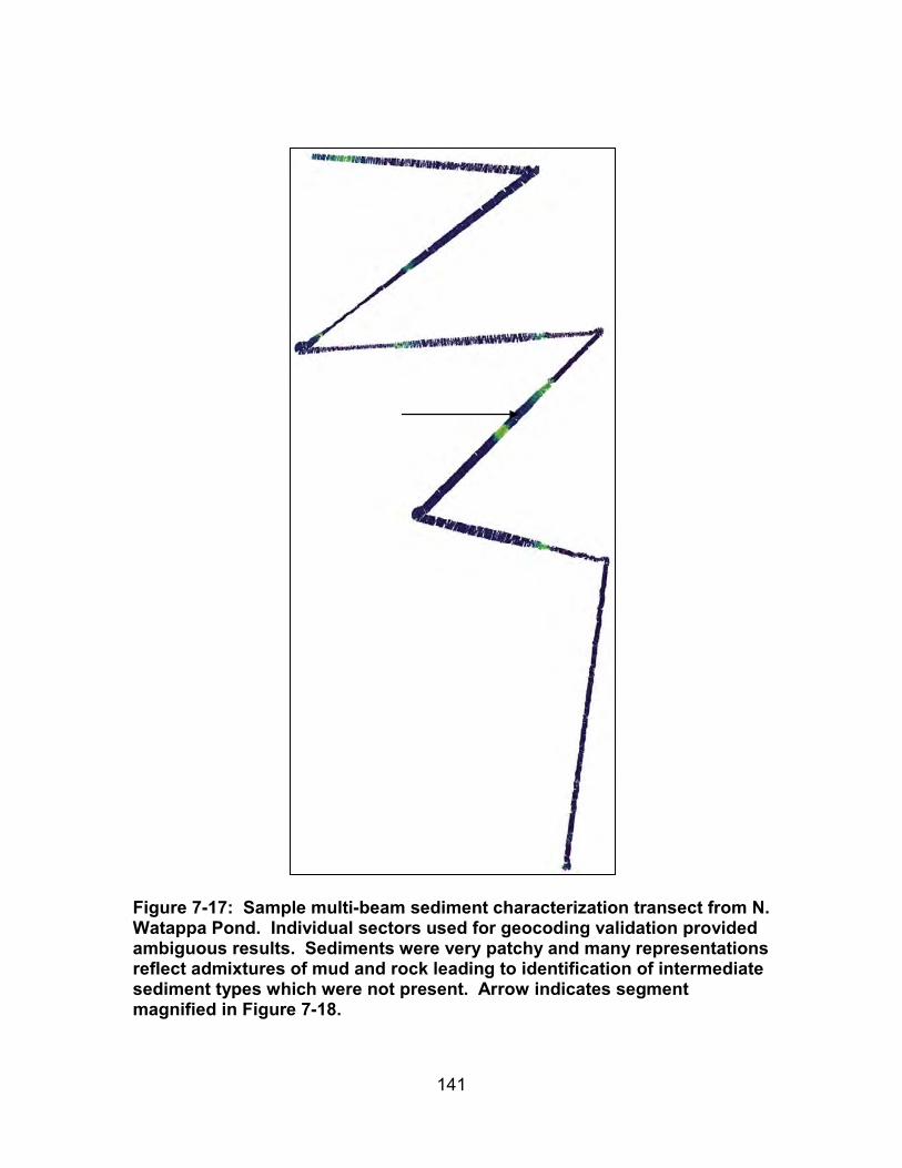
141

Figure 7-17: Sample multi-beam sediment characterization transect from N. Watappa Pond. Individual sectors used for geocoding validation provided ambiguous results. Sediments were very patchy and many representations reflect admixtures of mud and rock leading to identification of intermediate sediment types which were not present. Arrow indicates segment magnified in Figure 7-18.

142

Figure 7-18: Magnification of multi-beam survey line following sediment characterization.

7.7 Sediment Photography Photography provides greater resolution than acoustic imaging as well as color rendering and is an ideal way to assess sediment architecture and identify epifauna. In waters as shallow as 2 meters SCUBA gear is required to produce high quality images and the images are not easily geo-referenced to allow detailed work for time series studies. Initial work with the IVER2 utilized an integrated, high-definition camera with time stamps and geo-referencing synchronized with other measurements made by the vehicle. Later work relied upon a GOPRO Hero3 high–definition camera mounted to the bottom of the AUV. Photographs from the mounted camera could not be accessed by the AUV’s operating software, but the camera’s internal clock was synchronized with the AUV’s internal clock so that photographs could be precisely correlated with time-stamped positions generated by the AUV. The AUV was trimmed and ballasted to run 1m from the bottom at a speed of 1m/s. With this configuration, one square meter of sediment was captured with each photograph and a full coverage mosaic could be created. In practice,

143

photo-mosaics of the entire bottom were too memory intensive to generate, but known field of view and precise altitude control allowed calculation of epifaunal density (Figure 7-19). This setup was used repeatedly in Ashumet Pond, Falmouth, MA to determine the density and distribution of threatened fresh-water mussels to determine potential impacts on the population resulting from nutrient remediation activities (Figures 7- 20, 7-21).

Figure 7-19 Medium and high density mussel beds photographed from AUV in Ashumet Pond, Falmouth, MA.

Figure 7-20: Map showing Ashumet Pond transect lines for bottom photography in 2010. Yellow areas on map indicate the presence of live mussels in a single frame.

144

Figure 7-21: Mussel Survey transects assessed by AUV camera survey in 2012. The yellow and white dots represent way points with the connecting lines indicating the survey lines. The red lines indicate frames where freshwater mussels were observed. Transect locations were identical to those surveyed in 2010.

145

Figure 7-22: Light colored mantle and siphons visible in actively ventilating mussel represents the most important criteria for determining the community viability.

146

Figure 7-23: Side scan sonar survey (Yellow fin) performed concurrently with sediment photography provided images only during turns. Blanking distances were not compatible with low altitudes required for photography.

Transects separated by a distance of 15 m were performed in regions that had mussel populations identified from previous studies (Figure 7-20). Mussel populations were assessed before and after remediation efforts (Figures 7-20 and 7-21). Slow dissolution of empty mussel valves required close examination of the images to determine whether observed mussels were alive, and therefore part of a viable population, or dead. Image detail was sufficient to identify the siphons and light colored mantle of mussels actively filtering water and mussels in a normal life position. These criteria were verified by diver (Figure 7-22). Results demonstrated an apparent expansion of mussel habitat, though there is speculation that decreased sedimentation attributed to remediation efforts may account for higher visibility of epifauna.

147

Side scan sonar surveys run concurrently with the photographic bottom surveys were unsatisfactory. The sonar blanking distance was greater than the altitude above bottom required to provide photographic detail. As seen in Figure 7-23, the side scan images were only resolved when the AUV was at the surface (eastern side), performing turns or getting a GPS fix at the end of a survey line. Limited photographic surveys of submerged aquatic vegetation were also performed with the AUV specifically to determine the density and distribution of eel grass beds and benthic macro-algae. The surveys verified direct observations made by divers. Changes in the density and distribution of drift macro-algae were determined through time series observations. Although the study showed the efficacy of using an AUV, nearly all of the surveys were performed from a surface vessel as boat traffic and mooring fields hindered movement of the AUV and created a hazard for other vessels. Numerous attempts were made to automate the photographic analysis through the use of ImageJ software and user created open source modules. Neither mussels nor submerged aquatic vegetation were suitable candidates for automated identification; the one exception was eel grass. Software could not distinguish mussel valves from rocks. The presence of branching macroalgae was correctly identified only when very sparse and on top of a light background, such as sand. The principle drawback to using photography was the need for water clarity. Regular measurements within Ashumet Pond indicated an upper threshold for photography of around 10 µg/L chlorophyll. 7.8 Sub-bottom Profiling Sub-bottom profiling has not been instrumented on the AUV’s available to our group. Testing of a low power CHIRP system was initiated during the last few months, but implementation is many months away. Power consumption appears to be the primary concern. 7.9 Conclusions Autonomous underwater vehicles have advanced rapidly over the last decade. Prices have decreased to the point where they are generally available and competitive with shipboard instrumentation. AUV’s can be a cost effective alternative to traditional site characterization and monitoring that is required for the optimization, permitting, and monitoring of marine renewable energy sites. After extensive testing with a suite of variously instrumented example vehicles (OceanServer IVER2), AUV’s have been shown to match or exceed surface vessel alternatives as well as provide unique capabilities that enhance traditional methods. The compact, highly maneuverable AUV platform was ideal for surveying MHK sites. Regions deemed dangerous for ship and crew were easily surveyed with AUV’s and by descending below the surface, the number of suitable survey days increased at least 10 fold.

148

8 GEO-REFERENCING AND DATA MANAGEMENT 8.1 Technical Summary The data sets being developed during the various studies done under this contract were envisioned to require management particularly in the area of geo-referencing. Battelle Corporation was enlisted to meet any challenges identified by the various investigators. This effort was not funded under this contract but a reserve for the work was established under another MREC grant. However, it was soon discovered that geo-referencing as a data management requirement was advancing rapidly due to the increase in use of various global positioning based software packages and the challenges envisioned at the time of proposal never materialized. At several junctions in the program, particularly the program review at the end of year one, the investigators were queried as to whether they required any assistance and none identified a need. Additionally, during this time the Battelle entity with which we had proposed was reorganized and the participating group was disbanded. Therefore, no work was done under this topic area.

149

9 CONCLUSIONS Spatial resource assessment for offshore renewable energy is technology intensive. In order for offshore renewable energy to be competitive both the technology and its use must be cost effective. Throughout this report technologies used to monitor and assess wind, wave, current, and environmental resources have been examined to determine the best directions technology should pursue to provide cost effective tools for offshore renewable energy. Available technologies for assessing offshore wind resources were evaluated and compared. While two dominant technologies exist, LIDAR and SODAR, the investigators found that LIDAR holds the greatest promise for spatial assessment of offshore renewable energy resources. A great impediment for development of this resource is the cost of deployment which requires either a stable platform or ways to compensate for the movement of floating platforms. The latter is the preferred pathway for the future as it provides the greatest flexibility from site prospecting through to post installation monitoring. Traditional methods for assessing offshore wave resources rely on buoys with high deployment and maintenance costs or radar arrays which lack flexibility and often are at odds with the aesthetic ideals of coastal and beach communities. Smaller inconspicuous arrays were developed which can operate at multiple frequencies providing greater information in many varied conditions. In addition, traditional marine radars were modified and repurposed to provide similar information from ships farther out to sea. Both of these studies provide a path towards economical spatial assessment of offshore wave resources. Furthermore, these studies provide an example of how incentives for collaboration between industry and manufacturers can pave the way for technology development specific to the needs of offshore renewable energy. Development of new technology is not the only way to increase cost effectiveness. Doppler current data produced by existing technology was reexamined with reference to the specific needs of offshore wave and tidal current renewable energy. By reinterpreting data from horizontal acoustic Doppler current profilers it was found that invaluable near real time wave prediction was possible. Not only could these insights provide cost effective wave resource assessment, but if developed further, these insights could provide early warning of incoming damaging waves allowing time to protect wave energy converters. In addition, the same information could be used to optimize the efficiency of wave energy conversion to a constantly changing wave regime. Tidal current and environmental resources were assessed with available technology deployed from an AUV instead of using traditional ship mounted or towed arrays. It was shown that AUV technology has advanced to the point that they can provide data comparable to the best traditional methods. Furthermore, in the difficult, energetic environments characteristic of offshore renewable

150

energy sites, AUV’s were able to maneuver in critical regions safely, unobtainable by surface vessels. The initial capital cost of AUV’s has also decreased significantly allowing rapid cost recovery as a result of being able to use less personnel and smaller vessels to perform simultaneous surveys of multiple parameters. AUV’s point towards a future in which current velocity prospecting, as well as critical baseline environmental surveying, may be performed better, in less time and at lower expense than today. These studies have mapped out promising pathways to cost effective spatial resource assessment for offshore renewable energy ranging from wind to the benthos. The common thread throughout has been close collaboration between the manufacturers of required technology and the scientists and developers that use that technology. Fostering this collaboration provides incentive for manufacturers to focus limited resources towards finding solutions to problems specific to the needs of the maturing offshore renewable energy industry.

The Department of the Interior Mission As the Nation's principal conservation agency, the Department of the Interior has responsibility for most of our nationally owned public lands and natural resources. This includes fostering sound use of our land and water resources; protecting our fish, wildlife, and biological diversity; preserving the environmental and cultural values of our national parks and historical places; and providing for the enjoyment of life through outdoor recreation. The Department assesses our energy and mineral resources and works to ensure that their development is in the best interests of all our people by encouraging stewardship and citizen participation in their care. The Department also has a major responsibility for American Indian reservation communities and for people who live in island territories under US administration.

The Bureau of Ocean Energy Management As a bureau of the Department of the Interior, the Bureau of Ocean Energy (BOEM) primary responsibilities are to manage the mineral resources located on the Nation's Outer Continental Shelf (OCS) in an environmentally sound and safe manner.

The BOEM Environmental Studies Program The mission of the Environmental Studies Program (ESP) is to provide the information needed to predict, assess, and manage impacts from offshore energy and marine mineral exploration, development, and production activities on human, marine, and coastal environments.