fleet of intermodal containers carrying domestic freight on rail network in the u.s., mexico and...
TRANSCRIPT


Fleet of Intermodal Containers carrying Domestic freight on rail network in the U.S., Mexico and Eastern Canada.
Business Model is rail ramp to rail ramp Wholesale loaded moves (does not include the pickup and delivery components of the moves). Customers are IMC’s.
Objective is to maximize the ultimate return on the container assets. How to identify and capture more of the most beneficial freight in the network to drive the best total profit contribution from the fleet.


Variable contribution to fixed costs◦ Revenue (ramp to ramp paid by
IMC)◦ - Rail Linehaul (ramp to ramp paid to Rail)◦ Contribution
Other Network Costs◦ Container cost◦ Chassis costs◦ Maintenance & Repair of Assets◦ Repositioning costs (empty containers to next
load point)

City A City B ($300)
City A City C ($250)

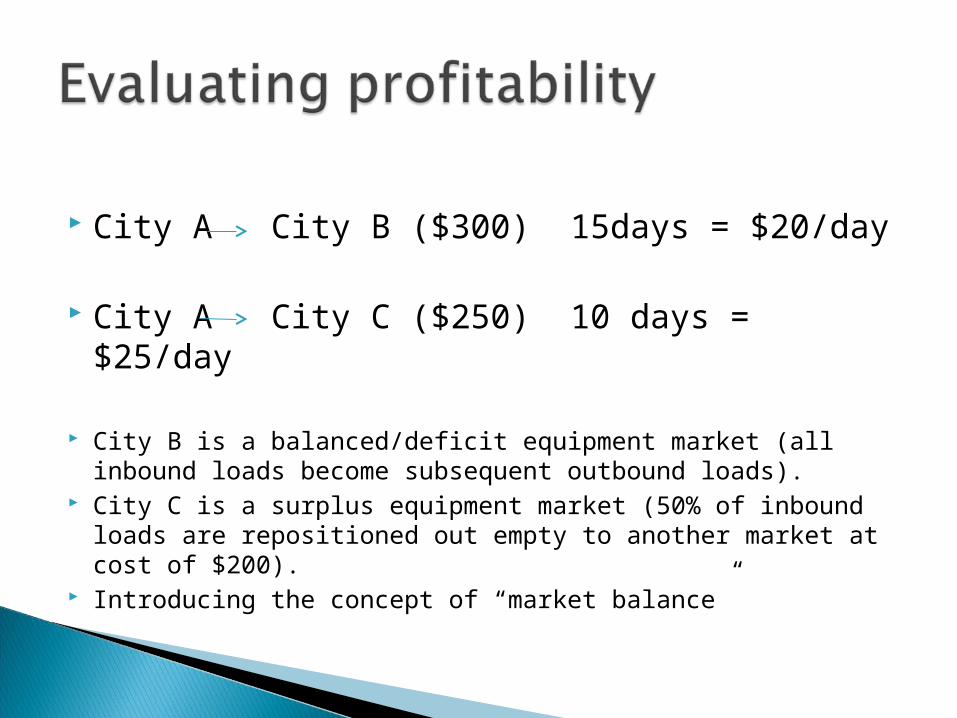
City A City B ($300) 15days = $20/day
City A City C ($250) 10 days = $25/day
Introducing the concept of “velocity”
Trip days include empty awaiting dispatch, pickup, rail transit, delivery, return of container.
Contribution/day more of a surrogate for return on investment
City A City B ($300) 15days = $20/day
City A City C ($250) 10 days = $25/day
City B is a balanced/deficit equipment market (all inbound loads become subsequent outbound loads).
City C is a surplus equipment market (50% of inbound loads are repositioned out empty to another market at cost of $200).
Introducing the concept of “market balance”

City A City B ($300) 15days = $20/dayCity B outbound loads avg. $250 contrib.
City A City C ($250) 10 days = $25/dayCity C outbound loads avg. $200 contrib.Surplus equipment is repositioned out at $200 cost to another market. Subsequent loads from that market avg. $500 contrib.
And so on………………

Each Market evaluated for Outbound CTB/day adjusted for empty repositioning costs out net of the subsequent load CTB at repo destination
100 Outbound Loads:
◦ 80 at $350 CTB; avg. $25/day (multiple destinations and customers)
◦ 20 repos at $200; subsequent load at $300; net=$100 CTB; avg. $5/day (including repo + load days)
◦ Load Center weighted avg. = $21/day

Drive more business into profitable Load Centers
Drive less business into less desirable Load Centers
“High Grade” business into surplus markets by choosing the best inbound business and handling less low end business (more important if total fleet is fully utilized)
Accommodate seasonality by viewing Load Center on Quarterly basis.

Sales Focus◦ Seek business into attractive Load Centers◦ Deemphasize growth into underperforming markets
Pricing◦ Establish pricing floors on new business in/out markets
to improve network profitability Repositioning
◦ Direct repo flows to most optimal market opportunities Equipment Dispatch
◦ Influence volume flows in support of network optimization. “Street turns” defeat next load discretion.

Total Contribution Per Period $5,400,000
Number of Containers
10,000
Contribution per Container/Period
$540
Loads per Container/Period
1.68
Contribution Per Load
$320
Empty Repo Cost/Load
$30
Empty to Load Ratio
10%
Unit Empty Repo Cost
$300
Contribution b4 Equip per Load
$350
Loads per Active Box
1.9
Active Inventory
89%
Total Inventory
10,000
Out of Service
Inventory 300/ 3.0%
Surplus Container Inventory
800/ 8.0%

Fleet Capacity Planning Empty Repositioning Network Balance (Including Spot Pricing) Network Directed Sales Network Pricing Guidance (Floors, Targets)
◦ At Capacity: High Grading, Velocity◦ Underutilized: Incremental Opportunities
Load Center Management (Cross-Functional Teams to Implement)

Using equipment dispatch to influence the network
Constraining dispatch to undesirable markets “Wait List” management (constrained
environment)◦ Customer priority◦ Destination priority◦ Dispatch Limits (allow “overdispatch” based on
historical gate turn data and customer behavior)◦ Equipment Specifications (limited to selected
customers or destinations)

Simulation to identify optimum flows/mix
Challenge in setting proper boundaries and constraints in the model (demand, limits, etc)
Work began but not seen through with change in the network business model
Provided some insights into opportunities that we had not fully considered previously.
Complexity of any modeling will be greatly increased by incorporating the “street” economics of the load pickup, delivery and empty miles.