ill a model to determine benefits obtainable from the ... · a model to determine benefits...
TRANSCRIPT

.. .
ill
A Model to Determine BenefitsObtainable from the ManagementI
i~7 of Riverine Fisheries of~~: . Bangladeshc.l
Mahfuzuddin AhmedtIP
.,
~
. 111][)t~IMINTERNATIONAL CENTER FOR LIVING AQUATIC RESOURCES MANAGEMENT
MANILA, PHILIPPINES
...

c/ A Jkkodel to Determine Benefits
06ainable from the Management of Riverine Fisheries of Bangladesh
Mahfuzuddin A med ,h
INTERNATIONAL CENTER FOR LIVING AQUATIC RESOURCES MANAGEMENT MANILA, PHILIPPINES

A Model to Determine Benefits g28
/ I 1 W i l
Obtainable from the Management of Riverine Fisheries of Bangladesh AX 1 1 1993
Printed in Manila, Philippines
Published by the International Center for Living Aquatic Resources Management, MC P.O. Box 1501, Makati, Metro Manila, Philippines through the financial assistance of the Ford Foundation, Dhaka; and Winrock International Institute for Agricultural Development, c/o the Bangladesh Agricultural Research Council, Farm Gate, Dhaka, Bangladesh.
Ahmed, M. 1991. A model to determine benefits obtainable from the management of riverine fisheries of Bangladesh. ICLARM Tech. Rep. 28, 133 p.
ISSN 01 15-5547 ISBN 971-8709-08-8
Cover: Small-scale fishing using liftnet in a small river adjoining the Jamlrna River near Dhaka, during the flood season, Bangladesh. Photo by M. Ahmed.
ICLARM Contribution No. 728.

CONTENTS
List of Tables ..............................................................................................................
List of Figures ...............................................................................................................
Foreword ......................................................................................................................
Abstract ........................................................................................................................
Aspects of the Riverine Fisheries in Bangladesh ..................................................
Chapter 1 . Introduction ................................................................................................
Resources Externalities and Economic Inefficiency in Open-Access Fisheries ................ Management Alternatives ..................................................................................................... Analysis of Existing Economic Models of Fisheries ........................................................... Conclusion .............................................................................................................................
Chapter 2 . Inland Fisheries of Bangladesh .............................................................
The Production System ........................................................................................................ Major Inland Fisheries ....................................................................................................
Hilsa Fishery ............................................................................................................ Carp Fishery ............................................................................................................. Giant Freshwater Prawn .......................................................................................... Floodland-Dependent Species .................................................................................
Production Organization and Dynamics of Fleet Operations ............................................. Demand Relations and Markets ........................................................................................... Management and Tenure: Their Implications ......................................................................
Chapter 3 . Methodology ..............................................................................................
Fundamental Relationships .................................................................................................. Product Market Equilibrium in Fishery ................................................................................ Structure of a Price Endogenous Fisheries Programming Model ......................................
Individual Model .............................................................................................................. Aggregate Model ............................................................................................................ Linear Programming (LP) Approximation ......................................................................
The Riverine Fisheries Model of Bangladesh ..................................................................... General Characteristics .................................................................................................. Objective Function .......................................................................................................... Activity Set and Constraints ..........................................................................................
Harvesting Block ...................................................................................................... Postharvest Handling Block ..................................................................................... Selling Block .............................................................................................................
Model Parameters and Functional Relations ................................................................ Bioeconomic Production and Market Submodels ................................................................
Bioeconomic Production and Fishery Supply ................................................................
iii
vii

Fishery Production Function .................................................................................... Biological Production .......................................................................................... Bioeconomic Production ....................................................................................
Fishing Effort and Its Internal Structure ................................................................. Production Models for the Riverine Fisheries of Bangladesh ......................................
Identification and Definition of Variables and Models ............................................ Specifications of the Econometric Model ................................................................ Gear Capacity and Methods of Standardization ..................................................... Cost Function ........................................................................................................... Components of Cost ................................................................................................
The Market Submodel .................................................................................................... Ex-Vessel Market ..................................................................................................... Wholesale Market ..................................................................................................... Retail Market ............................................................................................................ Specification of the Econometric Model .................................................................. Market Demand Equations ...................................................................................... Aggregation of Submarkets ..................................................................................... Functional Form and Choice of Variables ..............................................................
Price Differences Between Market Levels and Postharvest Cost ...............................
Chapter 4 . Parameter Estimation: Bioeconomic and Market Submodels ..........
Bioeconomic Submodel ........................................................................................................ Production and Cost Equations ..................................................................................... Data ................................................................................................................................ Estimation and Results ..................................................................................................
Market Submodel .................................................................................................................. Market Demand Equatpns and Data ............................................................................ Data Evaluation .............................................................................................................. Estimation and Results ..................................................................................................
Chapter 5 . Model Implementation: Results and Discussion .................................
Introduction ........................................................................................................................... Results of the Base Model .................................................................................................. Sensitivity Analysis ...............................................................................................................
Variation of Effort and Model Response ....................................................................... Simulation of Cost and Demand Changes and Implications for Policy .......................
Changes in the Cost of Harvest ............................................................................. Changes in Aggregate Demand ..............................................................................
Implications ...........................................................................................................................
Chapter 6 . Policy Implications and Conclusion ......................................................
Acknowledgements .......................................................................................................
..................................................................................................................... References
Appendices
A: Tables 33 to 54 ............................................................................................................... B: Questionnaire ................................................................................................................... C: List of Important Fish and Prawns Harvested
from the Riverine Fisheries of Bangladesh ...................................................................

LIST OF TABLES
Table 2.1. Areas of different types of fisheries and annual production in Bangladesh, 1988-89 ... 8 Table 2.2. Recent annual catches (t) of various species from the rivers of Bangladesh ............. 10 Table 2.3. Percentage share of annual iandings of different species from rivers in different
regions of Bangladesh, 1983-87. ............................................. ............................. ........... . . . . 12 Table 2.4. Seasonal share (%) of landings of different species from rivers in each region of
Bangladesh, 1983-87 ................... . .... ................ ........... . . . ........... . . . ................ . ........... . . . . . . . . 13 Table 2.5. Distribution of annual catch (t) from the rivers of Bangladesh by type of gear,
1985-86 . ....... . . ....... . ....... ............ . . . . . ........... .......... . .......... . . ............ . ................... ........... . . . . . . . 14
Table 3.1. A schematic of the LP Tableau for the riverine fisheries of Bangladesh ..................... 26
Table 4.1. Regression of average cost for a fishing unit in different riverine fisheries of Bangladesh . . . . . . . . . . . . . . . . . . . . . . . . . . . . . . . . . . . . . . . . . . . . . . . . . . . . . . . . . . . . . . . . . . . . . . . . . . . . . . . . . . . . . . . . . . . . . . . . . . . . . . . . . . . . . . . . . . . . . . . . . . . . . . . . 49
Table 4.2. Computed average cost equations for a hilsa fishing unit in various seasons in the riverine fisheries of Bangladesh .......................................................................................... 50
Table 4.3. Aggregate average cost equations for hilsa fishery in various seasons in the riverine fisheries of Bangladesh .......................................................................................................... 50
Table 4.4. Estimates of monthly retail demand models for various species harvested from the rivers of Bangladesh ............................................................................................................. 54
Table 4.5. Estimates of monthly ex-vessel demand models for various species harvested from the rivers of Bangladesh .................................................................................................. 54
Table 4.6. Price flexibility coefficients for retail demand parameters of various riverine species in Bangladesh ............................................................................................................................. 55
Table 4.7. Price flexibility coefficients for ex-vessel demand parameters of various riverine species in Bangladesh ............................................................................................................. 56
Table 4.8. Monthly retail demand equations for various species landed from rivers of Bangladesh ................................................................................................................................. 57
Table 4.9. Monthly ex-vessel demand equations for various species harvested from the rivers of Bangladesh ............................................................................................................................. 57
Table 5.1. Summary of results for the Base Model for riverine fisheries of Bangladesh ............. 61 Table 5.2. Distribution of catch (t) of various species and level of effort (gear hours x lo6)
in the Base Model for riverine fisheries of Bangladesh by river group .................................. 62 Table 5.3. Regional share of total landings and postharvest cost in the Base Model for
riverine fisheries of Bangladesh ................................................................................................ 64 Table 5.4. Aggregate values of different variables at various levels of total effort in the Base
Model for riverine fisheries of Bangladesh ............................................................................... 65 Table 5.5. Changes in effort (gear hours x lo6) availability for each fishery in the Base Model
for riverine fisheries of Bangladesh .......................................................................................... 69 Table 5.6. Shadow prices of effort for various fisheries (Dual value in million BDT) ................... 70 Table 5.7. Behavior of the riverine fisheries of Bangladesh under alternative cost conditions
(changes in the cost of harvesting from the Base Model) ...................................................... 71 Table 5.8. Total catch, price and effort for individual species under alternative cost conditions . 72 Table 5.9. Changes in the availability of effort for a 25% increase in the cost of harvest from
the Base Model for riverine fisheries of Bangladesh ............................................................... 73 Table 5.10. Changes in the availability of effort for a 2Soh decrease in the cost of harvest from
the Base Model for riverine fisheries of Bangladesh ............................................................ 74

Table 5.1 1 . Behavior of effort (gear hours x lo6) use and landings (t) of individual species at various levels of effort availability and under alternative cost conditions ............................... 76
Table 5.12. Shadow prices (BDT x 106 per gear hour x 109)of effort under alternative conditions ....................................................................................................................... of cost of harvest 77
Table 5.13. Behavior of different riverine fisheries of Bangladesh under alternative demand conditions (changes in the demand intercept from the Base Model) ...................................... 78
Table 5.14. Total catch, price and effort for individual species under alternative demand conditions .................................................................................................................................... 78
Table 5.15. Changes in the availability of effort for a 10% decrease in the aggregate demand from the Base Model for riverine fisheries of Bangladesh ..................................................... 79
Table 5.16. Changes in the availability of effort for a 10% increase in the aggregate demand from the Base Model for riverine fisheries of Bangladesh ...................................................... 81
LIST OF FIGURES
Fig . 2.1. Map of Bangladesh: river systems and geographic regions .............................................. 7 Fig . 2.2. Seasonal changes in the biology and fisheries of fish and prawns in the open waters
of Bangladesh ............................................................................................................................... 9 Fig . 2.3. Percentage composition of average yearly catch in the rivers of Bangladesh,
.................................................................................................................... 1 983-84 to 1 988-89 14 Fig . 2.4. Main marketing channels of fresh fish from the inland open waters of Bangladesh ...... 15 Fig . 2.5. Monthly average retail prices of major riverine species in Bangladesh, showing
seasonal trends and overall price increases over time ............................................................ 15 Fig . 2.6. Capture of fish and number of fishers in the inland fisheries of Bangladesh ................ 17
Fig . 3.1. Fundamental relationship between catch, effort and cost in a fishery ............................ 20 Fig . 3.2. Market equilibrium of fishery sector in a supply-demand model ...................................... 21 Fig . 3.3. Segmentation of demand and benefit functions for linear programming . .
approxlmatlon .............................................................................................................................. 27 Fig . 3.4. Short-run yield curves as a function of nominal efforts ............................................. 37 Fig . 3.5. Short-run total cost as a function of fish output ............................................................... 37 Fig . 3.6. Short-run average and marginal cost curves for fish output ............................................ 38 Fig . 3.7. Long-run average cost curve of fish output in a steady-state fishery ............................. 38 Fig . 3.8. Relationships between market levels in terms of marketing margins of fish output ....... 46
Fig . 5.1. Comparison of Base Model landings and official landings from the rivers of Bangladesh. 1983-84 to 1986-87 . A . by species groups; B . by river groups ......................... 63
Fig . 5.2. Aggregate catch and effort relationships in the Base Model ........................................ 66 Fig . 5.3. Benefit, cost and effort relationships in the Base Model ................................................ 66 Fig . 5.4. Benefit, cost and catch relationships in the Base Model ................................................. 66 Fig . 5.5. Shadow prices of effort in the Base Model ...................................................................... 66 Fig . 5.6. Catch and effort relationships for individual groups in the Base Model .......................... 67 Fig . 5.7. CPUE and effort relationships for various groups in the Base Model ............................ 68 Fig . 5.8. Shadow prices of effort for various fisheries in the rivers of Bangladesh ...................... 68 Fig . 5.9. Catch and effort under alternative cost conditions ........................................................... 74 Fig . 5.10. CPUE and effort under alternative cost conditions ......................................................... 74 Fig . 5.1 1 . Gross benefit and effort under alternative cost conditions ............................................. 74 Fig . 5.1 2 . Cost and effort under alternative cost conditions ........................................................... 74
........................... Fig . 5.1 3 . Net benefit and effort relationships under alternative cost conditions 75 Fig . 5.1 4 . Shadow prices of effort under alternative cost conditions ............................................. 76 Fig . 5.15. Catch and effort under alternative demand conditions ................................................... 80 Fig . 5.16. CPUE and effort under alternative demand conditions .................................................. 80
...................................... Fig . 5.1 7 . Gross benefit and effort under alternative demand conditions 80 Fig . 5.1 8 . Cost and effort under alternative demand conditions .................................................... 80
..................... Fig . 5.19. Net benefit and effort relationships under alternative demand conditions 81 ....................................... . Fig 5.20. Shadow prices of effort under alternative demand conditions 82

CHAPTER 1
INTRODUCTION
The pervasive tendency of open-access fisheries to expand effort to the point where resource rent is dissipated, first pointed out by Gordon (1954) and then by many others after him, has been a major cause of concern within the sector all over the world. In many fisheries, the tendency to overexploit the resources has driven stocks to levels below their (maximum yield) potential and has worsened economic conditions of the fishing communities depending on these resources.
The fisheries of Bangladesh contribute 71% of the animal protein supply of the country. Nearly one-tenth (1 0 million) of the country's population is involved as part-time and full-time workers in fishing and related activities. The inland fisheries employ nearly one million full-time fishers (BBS 1986; World Bank 1991).
The conditions of the inland capture fisheries of Bang!adesh have deteriorated in recent years and production has either stagnated or even decreased for some major species (DOFIBFRSS 1985, 1986, 1991). On the other hand, the fishing-dependent population has been on the increase, signifying a mounting pressure on the available fisheries resources (BBS 1989 and previous issues). The traditional system of administering fisheries activities is insufficient to maintain production from the various fisheries and, more importantly, to the task of maintaining the flow of benefits that the fisheries are capable of generating.
In Bangladesh, most of the inland fisheries exploitation activities are small-scale and traditional. Over the years, these fisheries have retained an open-access character in the absence of a consistent and effective management policy. For a long time the fisheries had been managed by a group of middlemen who secured yearly leases from the government through auctions. Consequently, an increasingly large fishing dependent population and an excess fishing effort relative to the availability of stock have contributed to declining catches of some or all species and a deteriorating fishing income. These fisheries will require some kind of control of effort in order to improve their economic performance.
In response to these problems, a comprehensive policy for inland fisheries management is in the process of implementation by the government. The objective of this New Fisheries Management Policy (NFMP) is mainly to redirect the potential benefits of fisheries exploitation activities to "actual fishers" and at the same time maintaining and improving the productivity of the fisheries on a sustainable basis. In this effort, a system of licensing of water bodies to actual fishers or groups of fishers has been introduced in selected areas of inland fisheries. This would replace the traditional system of leasing out the water bodies to private individuals. The economic consequences of these new practices are yet to be addressed (Aguero et al. 1989).
A major problem confronting management policies is the determination of the type and level of control which should be applied to the fisheries in order to achieve best the above objectives. This necessitates the understanding of the performance-response of the fisheries to alternative management policies in terms of the resultant impact on the beneficiaries or users of the resources, i.e., the fishers, the trading community and the consumers.

The principal objective of this research was to develop a bioeconomic model that would provide a basis for assessment of economic consequences of various alternative management measures for the inland fisheries of Bangladesh.
Resources Externalities and Economic Inefficiency in Open-Access Fisheries
In an open-access fishery, benefits tend to be dissipated because whenever a positive benefit occurs (as in a newly developing fishery or with an increase in the price for the product), additional factor inputs of labor and capital are attracted. This tends to continue until revenue per unit of fishing effort is equated to the level of its marginal opportunity cost (Scott 1955; Copes 1972; Munro and Chee 1978; Christy 1982). The exploitation of fishery resources under open-access conditions, as such, will result in a suboptimal allocation of resources as far as strict economic efficiency is concerned. This was established in the seminal work on fisheries economics by Gordon (1954), by introducing economic variables into the logistic model of population growth in fisheries of Schaefer (1954).
Uncontrolled access to fishing stocks induces fishers to compete among themselves for available fish resources. As a result, there is little incentive for individual fishers to restrict their fishing effort in the general interest of maintaining fish stocks since any fish that an individual fisher leaves in the water may be captured by another fisher. This situation results in dissipation of the economic rent that resources can generate, through overcapitalization and overfishing. As such, we find the industry characterized by production costs that are excessive relative to the value of production. Fishers, therefore, eventually find themselves in an untenable position with considerable investment in vessels and equipment that cannot be instantly liquidated (Cauvin 1979). In small-scale fisheries of developing countries, investments are not as great as in large-scale fisheries, but the results are the same as there are few employment opportunities consistent with their skills and experience.
Second, as a result of excessive fishing effort, and despite harvest control measures, fisheries resources are subject to overexploitation (Scott 1979). Finally, the potential economic value of the resource to society in the form of a resource rent becomes dissipated (Cauvin 1979). This is a classic case of the "Tragedy of the Commons" (Hardin 1968).
Various forms of externalities result from open competition in the harvesting sector of the fishery. They include: (i) crowding externalities due to vessel congestion on fishing grounds; (ii) misallocation of effort among species and fishing grounds; and (iii) distortion in the use of factors of production, e.g., incentive to adopt new technologies faster than is socially desirable (Greboval 1985).
Management Alternatives
The literature on fisheries economics divides fisheries regulations into two broad categories: conservation measures to protect and enhance stock productivity and management measures aimed at economic efficiency.
Conservation measures such as closed season or area and control of mesh size have received considerable attention by fisheries regulatory authorities. For instance, following the conceptualization of eumetric fishing by Beverton and Holt (1957), the control of mesh size became a very popular regulatory instrument. The consequence of eumetric fishing is to increase the yield and biomass; the latter being important if

FOREWORD
The present document is based on a thesis in resource economics presented at the Faculty of Economics and Management, Universiti Pertanian Malaysia, Kuala Lumpur, in July 1989.
In the course of his thesis work, Dr. M. Ahmed spent, besides the obligatory field work in Bangladesh, his homeland, a period of almost three years at ICLARM Headquarters in Manila from 1986 to 1988, both to learn from and contribute to various projects related to his work, and conducted by other ICLARM staff, notably Dr. M. Agiiero and Ms. A. Cruz- Trinidad.
It is now with considerable pleasure that I introduce this document - our first Technical Report devoted to Bangladesh - to its readers. It illustrates - if need be - that economists have much to contribute to fisheries research and management. Indeed, such a comprehensive view of the freshwater fisheries of Bangladesh as presented in this document has never been elaborated by the biologists - local and expatriate - who have studied the inland fisheries of Bangladesh: the biologists have tended to concentrate on details of the biology of the resources species and to forget the "big picture".
This big picture, as presented to us by Dr. Ahmed, is that the fisheries in question are extremely valuable and could generate, under the optimal conditions he identifies, a net surplus of nearly 1.4 billion Taka, i.e., over US$40 million per year. He also identifies and quantifies the main constraint to the realization of this surplus: excess fishing effort, the plague of the world of fishing.
Finally, he presents a cogent case for the implementation of the New Management Policy promulgated by the Government of Bangladesh, as well as providing guidelines for further studies.
I can only hope that this document will find, among decisionmakers and scientists alike in Bangladesh and elsewhere, an attentive readership. Comprehensive studies such as that presented here are few and far between.
Dr. DANIEL PAULY Director Capture Fisheries Management
Program International Center for Living
Aquatic Resources Management

A Model to Determine Benefits Obtainable from the Management of Riverine Fisheries of Bangladesh
MAHFUZUDDIN AHMED International Center for Living Aquatic
Resources Management (ICLARM) MC P.O. Box 1501, Makati Metro Manila, Philippines
ABSTRACT
An operational model was derived which can be used to analyze the performance of Bangladesh riverine fisheries under different simulated alternatives of technical, economic and biological conditions.
Functions and parameters of a Base Model were estimated by deriving two submodels: (a) bioeconomic production and (b) the market, using regression techniques. Both primary and secondary data were used for empirical estimation of the submodels.
The model was developed in a linear programming framework to represent various fisheries in the riverine waters of Bangladesh. Results of the Base Model suggest that the riverine fisheries of Bangladesh are capable, under optimal conditions, of generating a total net benefit of BDT (Bangladesh Taka) 1,383 million per annum (US$1 = BDT32), of which 96% would accrue as producer surplus. Also, a significant overcapacity (118%) exists in the existing fleet in terms of application of effort relative to the resource availability.
Simulation of cost and demand changes reveal that the effect of changes in the cost condition of harvest will in general be related negatively to the intensity of total effort use, total landings, benefits and costs while the effects of changes in the aggregate demand on total effort, total costs, landings, prices and net benefits will be positive. The implication of the results for management is that intervention into the fisheries through control on effort intensity would produce substantial net benefits from the fisheries.
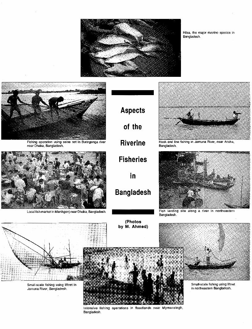
Hilsa, the major Bangladesh.
riverine species in
Fishing operation using seine net in Buringonga river near Dhaka, Bangladesh.
Local fish market in Manikgonj near Dhaka, Bangladesh.
Aspects
of the
Riverine
Fisheries
in
Bangladesh
(Photos by M. Ahmed)
Hook and line fishing in Jamuna River, near Aricha, Bangladesh.
Fish landing site along a river in northeastern Bangladesh.
Intensive fishing operations in floodlands near Myrnensingh, Bangladesh.

recruitment is stock dependent. However, in an open-access fishery, the rent created by eumetric fishing will only induce additional entry and the basic problem of economic inefficiency will persist (Turvey 1964). Therefore, these traditional forms of control may help protect stocks from destructive forms of effort, but are ineffective in regulating the amount of effort. In fact, severe overcapitalization occurred in some world fisheries as a consequence of measures such as catch quotas or closed seasons or areas (Crutchfield 1965; Greboval 1985). In addition, these measures (catch quota, season and area closure) affect the processing and marketing sector of the fishery by inducing peak and slack processing times, increased inventories and freezing, and price distortions (Anderson 1977). Thus, economists have tended to rely on management measures that reduce total inputs (effort) for any given catch level and encourage least- cost combination of inputs. Such measures include taxes, limited entry and quotas.
Theoretically, with an appropriate tax, fisheries could be left to the market without fear of biological depletion, of excessive inputs in general, or of the incorrect combination of inputs (Crutchfield 1979). Either inputs (effort) or output (landings) may be taxed. However, in order to produce its fullest effect, taxes must be factor-neutral (Crutchfield 1979). In this respect, a tax on landings makes a better impact. In addition, McConnell and Norton (1978) suggest that differential landing taxes in a mixed-species fishery could improve economic output significantly by making use of the fishers' self- interest and their limited ability to alter the species mix in their catch.
Finally, taxes serve as means of offsetting any adverse effects on the distribution of wealth, income or employment; taxes could be used to convert the social costs of management to an explicit charge on the productive activity of the participants.
There are, however, at least two practical difficulties with using taxes. First, they are politically infeasible in most parts of the world. Second, if taxes were used they would have to be dynamic, changing frequently, causing enormous administrative difficulties (Moloney and Pearse 1979).
Entry restriction reduces fishing inputs directly, by restricting fishing to holders of a legal right of access - a license, permit, or other legal evidence that a particular vessel and crew may use the resource. However, entry restrictions must be in terms of a limit upon one or more of the measures used in the industry. This is because rationing the supply of any resource used in the industry through entry restrictions will invite substitution of other resources for it (Turvey 1964).
Experiences with limited entry programs in many fisheries across the world have proven to be ineffective because some of the unregulated dimension of the fishing effort expanded to such an extent that substantial overcapitalization (capital stuffing) had occurred and much of the potential rents were eventually dissipated (Fraser 1979; Meany 1979; Pearse and Wilen 1979; Copes and Cook 1982).
There are exceptions. Newton (1978) acknowledged the growth of excess capital under limited entry in British Columbia fisheries with qualifications. Also, Meany (1979) citing the cases of rock lobster and shrimp fisheries of Australia under limited entry programs showed that there has been less tendency of overcapitalization and, hence, little dissipation of resource rent in shrimp fisheries compared to lobster fisheries.
In tropical multispecies fisheries, limited entry programs by license limitations and vessel and gear restrictions have been used to restrict catch level and to change catch compositions in order to prevent overexploitation (Beddington and Rettig 1983; Majid 1984). Although the success of such measures have not been fully assessed, Yahaya (1988) in discussing the issues and constraints of fishery management and regulation in Peninsular Malaysia, pointed out that license limitation may also lead to operating inefficiency among licensed vessels through increase of unregulated dimension of effort.

The third alternative in regulating exploitation intensity would be to create rights to specific quantities of fish (individual quotas) rather than simple rights to participate in the fishery through vessel or personal license. Under an individual quota system there is no incentive to overinvest in the vessel and gear. This would avoid some of the regulatory problems encountered in limited entry licensing, the dilemma between restricting technology to check capital stuffing through socially inefficient increase in fishing capacity and allowing free play to promote socially efficient cost reducing techniques.
The quota holders will select the least cost combination and deployment of inputs, including technological improvement and innovation without subjecting the resource to a surge of new fishing mortality (Crutchfield 1979). In addition, harvest glut can be avoided or reduced and a higher value of sales achieved by optimally meeting the time patterns of demand over the year (Copes 1986).
Despite the superiority of quotas, especially over limited entry licensing (see Christy 1973; Moloney and Pearse 1979; Scott and Neher 1981), in practical management terms, deliberate application of individual quotas are not seen free of defects. Copes (1986) gave an exhaustive list of areas where individual quotas face problems of implementation. Most of them are relevant for tropical fisheries where the operations are small scale with numerous actual and potential marketing channels and geographically widely dispersed activities.
In the case of inland fisheries of Bangladesh, thousands of small boats land their catches at hundreds of places and sell directly to the public at numerous local markets. Monitoring and enforcing any kind of limits on inputs and outputs would appear impossible. However, a limited entry program through licensing may still conform to ease of implementation and flexibility compared to taxes and quotas. The fear of capital stuffing through overinvestment in unregulated dimension of effort would be minimal, since the fisheries are mainly traditional and nonmechanized.
Analysis of Existing Economic Models of Fisheries
Fisheries are complex systems, consisting not only of the stocks of fish species and their surrounding environment, but also including the mechanisms of harvesting, processing, transporting and marketing activities, as well as the social and institutional setup under which the economic organization of the fishing industry takes place (Charles 1988). A multidimensional approach has to be adopted for capturing the essence of its various aspects, e.g., production, population dynamics, marketing and property systems.
Certain types of models, each used separately, could not suitably deal with the problem at hand. Each of them could only represent a part or subsystem, e.g., production, fish population, marketing and management, of the entire fishery process.
Several approaches to analyzing the implications of various management schemes are available. Mathematical models of the fishery which include biological and some economic factors have been found to be useful tools for determining the best regulatory scheme. Some familiar examples of these models are given by Schaefer (1954, 1968), Beverton and Holt (1957), Ricker (1 958), Larkin (1 963, 1966), Pella and Tomlinson (1969) and Fox (1970).
However, the above models dealt mostly with biological parameters and describe how fisheries (often a single-species fishery) change with time under a steady-state situation, whereas, in most cases fisheries operate under complex biotechnological and
socioeconomic conditions. The inclusion of these factors in the analysis results in multivariable models which are complex.
Much of the previous analysis of fisheries is based on the concept of an equilibrium, e.g., the maximum equilibrium yield analysis. Such an equilibrium is an idealization and is never encountered in reality because of the continually changing environment which acts as a disturbance and thereby displaces the system from its equilibrium conditions (Palm 1975). Moreover, the steady-state models may lose their applicability in complex fisheries when the time dimension is considered.
Unlike biological fishery management models, most of the fisheries economics models dealing with management problems were cast largely in static terms, based on a theory of fisheries management founded by Gordon (Clark and Munro 1975). Scott (1955) viewed fish population and biomass as a capital stock, capable of yielding a sustainable consumption flow through time, and thus attempted to cast the problem of management of a fishery resource as a problem in capital theory. This was followed by Crutchfield and Zellner's (1962) formulation in terms of a dynamic mathematical problem.
Optimization techniques, to maximize or minimize a particular function, may involve either linear or quadratic programming. Zellner (1961), Rothschild and Balsiger (1 971), Mueller et al. (1979) and Aguero (1987) applied linear programming to the economics of fisheries management. Mueller and Vidaeus (1981) developed a quadratic programming model for an optimal fishery strategy. The problem can be set either in a static or a dynamic frame. A simple dynamic approach was used by Rothschild (1971), who optimized the route of a fishing vessel. Quirk and Smith (1970) applied a time dynamic programming model to economic optimization of a fishing industry. Booth (1972) developed a discrete time-profit maximizing model. More recently, Wang and Mueller (1981) developed a model that deals with intertemporal issues and economic analysis in fisheries management. Palm (1975) showed the use of a static optimization method in conjunction with a dynamic method as a total approach. In this method, maximization is first done with static methods and then a feedback control function is constructed to keep the system near the resulting equilibrium condition.
In selecting models, several considerations have to be made. For instance, if the multispecies fishery characteristics call for an interactive approach, analytical models are more appropriate than single-species production models based on catch and effort data derived for a multispecies fishery (Greboval 1985). Another consideration is the data requirement of analysis. For example, in multiple strategy fishing, the catchability coefficient (fraction of stock removed by a unit of effort) can be better estimated using cluster analysis. However, the need for intensive data renders the use of such methods impracticable (Greboval 1985).
Technologocial interaction and mixed harvest strategy would yield an optimal harvest rate for the aggregate of stocks different from the theoretical maximum of each ,+
individual stock. However, if economic yield is maximized by equating marginal cost of fishing effort to the marginal revenues of a mixed catch, an optimal mix of production is achieved. Proper bioeconomic management of multispecies fisheries, therefore, requires control of overall amount of effort and some degree of control over the mix of production. An interactive method can be applied to achieve such objectives. Optimization techniques have been used for economic optimization of mixed stocks by several authors, e.g., Quirk and Smith (1970), Anderson (1975), Meuriot (1981), Aguero (1 983) and Logan (1984).

Conclusion
The situation in Bangladesh warrants developing or devising methods that will take proper account of the problem of poor quality data and the complex interaction of various factors, e.g,, technological interaction and mixed species harvest. It is important that the fishery process be represented by a model that is flexible and powerful enough to accommodate data and information gaps. A mathematical programming approach is considered appropriate and suitable because:
(i) it can handle a large number of variables of complex interdependence; (ii) the objective function (e.g., maximization of consumer plus producer surplus) can
measure the achievement of management objectives; and (iii) the model is capable of identifying an optimal strategy for allocation of effort in a
mixed-species harvest with geographical and seasonal variability in the species distribution.

CHAPTER 2
INLAND FISHERIES OF BANGLADESH
Bangladesh is a huge delta of 144,000 km2 formed by three main rivers: the Padma (Ganges), Meghna and Jamuna-Brahmaputra and their tributaries (Fig. 2.1). The size of the riverine (flowing river and estuaries) and other large inland perennial water bodies has been estimated to be about 12,200 km2, i.e., over 8OlO of the area of Bangladesh (Table 33 in Appendix A). The major fisheries take place in: (a) rivers and estuaries, (b) beels (natural depressions) and baors (dead rivers), (c) floodlands (seasonal floodplains) and (d) an artificial lake (Kaptai Lake).
The Production System
The inland capture fisheries are tightly bound to the pattern of the floodings which take place during the monsoon season. The yearly inundation of the countryside connects all the aquatic areas into one production system for up to four months (July-October). It is during this season that a major expansion in both numbers and biomass of fish takes place. Some of the major carps (Cyprinidae) and various floodland-dependent species spawn then and the fry spread all over the flooded area during this period. The ability of the fisheries to sustain themselves depends on extensive systems of interconnected areas of aquatic habitat that provide for reproduction and growth.
Estimates of the annual fish production from various water environments and area under each environment are shown in Table 2.1; a total of 424,140 t of fish were produced in 1988-89 from four million
Nathwest Region ,
0 Northeast Region - lnternationol boundary
Southwest Region ---- Region boundary
Southeast Region \< Rivers '+ I I I i
E 89"E 90°E 9i0E 92"E 9
Fig. 2.1. Map of Bangladesh: river systems and geographic regions.
hectares of inland open-water area. Moreover, the area of land intermittently inundated during the monsoon season to a depth of 30 cm or more (sufficient to support fish production) is estimated to be about 5.5 million ha (MPOIHARZA 1985b). Hilsa (Hilsa ilisha), carps (e.g., rohu Labeo rohita, catla Catla catla, mrigal Cirrhinus mrigala and kalbasu Labeo calbasu) and a few floodland-dependent species like catfish (e.g., "boal" Wallago attu, "pangas" Pangasius pangasius, "air" Mystus aor) and different types of prawns (Macrobrachiurn spp.) are the important species in the inland open waters. The

Table 2.1. Areas of different types of fisheries and annual production in Bangladesh, 1988-89. (Source: DOF, unpubl. data)
Area Production Yield Subsector of fisheries (ha.1o3) (t.10~) YO (kg.hal)
Inland fisheries Open waterlcapture
Rivers and estuaries Sunderban Beels Lake Kaptai Floodlands (seasonal)
Subtotal Closed water
Baors Ponds Coastal aquaculture
Subtotal Total inland Marine fisheries
Industrial (trawl) Artisanal Total marine
Grand total
major harvest periods of some economically important fish of Bangladesh are presented in Fig. 2.2. In general, except for hilsa, harvests from rivers take place in the postmonsoon period. The peak harvest of hilsa is during the spawning migration in the late monsoon period (August-October). A list of important fish is contained in Appendix C.
The annual or seasonal beels, which either dry up or are dried intentionally, are completely harvested each year during postmonsoon months. The permanent beel is a shelter fishery, and under the current management system, harvest is recommended only every third year to allow the fish populations to recover.
Harvest of the floodlands fish is done mainly for subsistence throughout the monsoon months (June through September). The peak harvest generally occurs during periods of receding or rising water when fish are trapped while coming to or going from the floodlands. The annual fish harvest from the floodlands through subsistence fishing has been estimated at 186,130 t in 1988-89 (Table 2.1), and as many as 10.8 million (73%) households were involved in these fishing activities in 1987-88 (World Bank 1991).
On the other hand, riverine fisheries are important for small-scale commercial fishing year-round. The total area of river environments scattered all over the country is 10,316 km2 producing about 181,140 t of fish annually (Table 2.1). Table 2.2 shows the production figures for different species in the riverine waters (rivers and estuaries). Hilsa is the dominant species, amounting to about 44% of the average annual riverine fish production (Table 2.2).
Major Inland Fisheries
HILSA FISHERY
The hilsa, an anadromous fish (i.e., migrating from the sea into rivers to spawn), is found in the foreshore areas, estuaries, brackishwater lakes and freshwater rivers of

Jan Feb Mar Apr May / ~ u n / Jul j Aug ; Sep j Oct i Nov Dec
Spawn~ng mlgratlon 1 1 1 l l l
Spawn~ng rn Seaward mlgratlon of
adults I I I I I I 3 Riverme harvest I I -I---
Estuar~ne residence and 1 1 - harvest at sea I 1 1 1 1 1 1 1 1
D~spersal of young In I ' I I I I rivers (downstream) 1 I I / I I I I
I I I I I I
Spawn~ng mlgratlon Spawn~ng
- I I I I I
m Dispersal of young over -+I I I
floodpla~n I I I I I I
? Return of young to -
beel and rlver I I I I
Hamest ln beel and I I 1 1, rlver Indry season I I I / / !-
Harvest dur~ng spawnlng mlgratlon A ! ! ! ! !
Lateral mlgratlon to I I I I I I floodpla~ns 1 1 1
C Reproduct~on - 1 1 D~spersal and growth &-I
o w Return to stand~ng water Harvest
g Dry season res~dence In standmg water
I I I I I I I 1 1 1 1 1 1 1
M~grat~on to estuary I I I I I I
% $ , Spawnmg In estuary I l l 2 2 2 Juven~le mlgratlon to
I l l fresh water
2 b 2 Feed~ng d~spersal mto & S k? - floodpla~n 3 - Hawest - <
I I I I I I
Fig. 2.2. Seasonal changes in the biology and fisheries of fish and prawns in the open waters of Bangladesh (Source: MPOIHARZA 1985a).
South and West Asia. The largest yields of hilsa fishery come from the deltaic region of the Gangetic system of India and Bangladesh. Of the three countries in the upper Bay of Bengal region (India, Bangladesh and Burma), where hilsa forms a commercial fishery, Bangladesh secures the largest share (more than 80%) of the landings, about 150,000 tyear-I from its inland river systems and inshore waters (Raja 1985; Islam 1989). In Bangladesh, the share of riverine production is at present less than 50% of the national production of hilsa (World Bank 1991).
No scientific assessment has been made so far on the population distribution of the various stocks of hilsa in the rivers, estuaries and inshore marine waters of Bangladesh (Dunn 1982). However, the dominant age and size in the population distribution is believed to be 1+ to 2+ years and 25-40 cm, respectively (Raja 1985). Normally, hilsa attains maturity at the age of I+ year when it has reached a size of 25-30 cm. Two principal breeding runs have been reported in Bangladesh, one during the southwest monsoon (June-October) and the other during winter (November-March). The latter is of smaller magnitude (Raja 1985).
The fishing season of riverine and estuarine stocks extends from June to March, with a major peak in September-October and a minor one in February-March. In 1988- 89, over 81,000 t of hilsa were harvested from various inland rivers and estuaries, 68% of which came from the principal river, Meghna (Table 2.2). The fishery belongs to the artisanal sector using mainly gillldriftnets and operates with the help of traditional
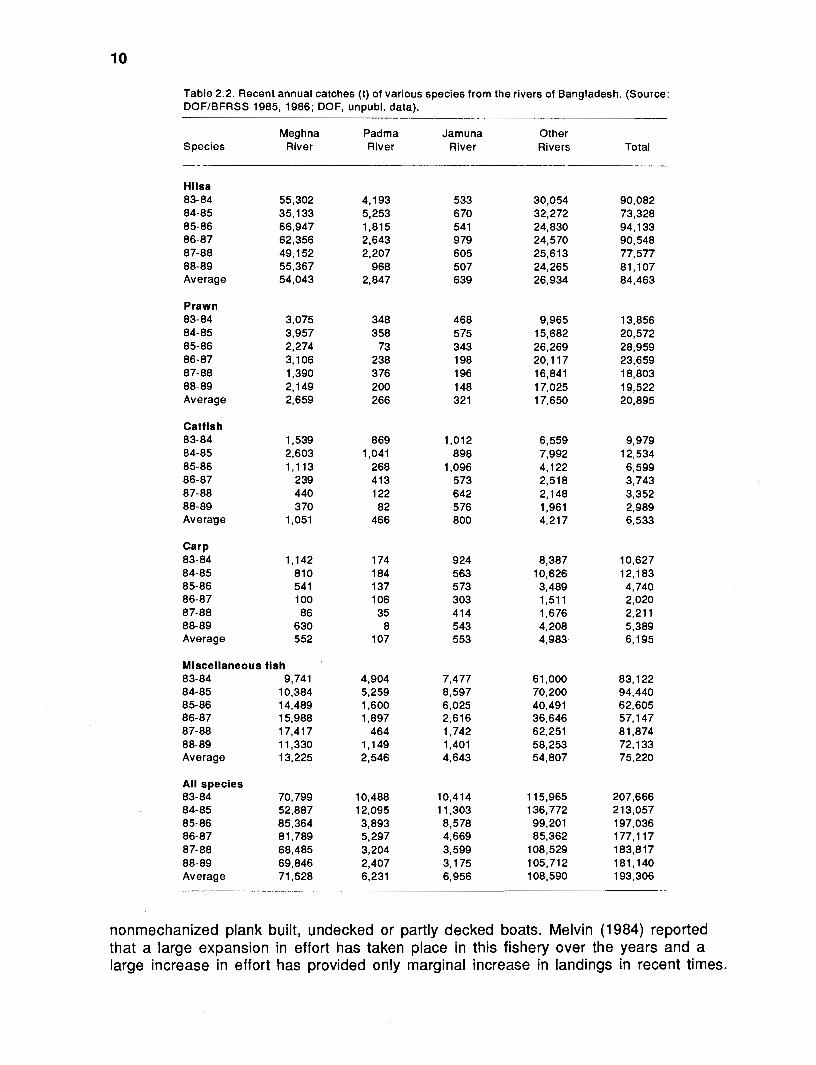
Table 2.2. Recent annual catches (t) of various species from the rivers of Bangladesh. (Source: DOFIBFRSS 1985, 1986; DOF, unpubl. data).
Meg hna Padma Jamuna Other Species River River River Rivers Total
Hilsa 83-84 84-85 85-86 86-87 87-88 88-89 Average
Prawn 83-84 84-85 85-86 86-87 87-88 88-89 Average
Catfish 83-84 84-85 85-86 86-87 87-88 88-89 Average
Carp 83-84 84-85 85-86 86-87 87-88 88-89 Average
Miscellaneous fish 83-84 9,741 84-85 10,384 85-86 14,489 86-87 15,988 87-88 17,417 88-89 11,330 Average 13,225
All species 83-84 70,799 84-85 52,887 85-86 85,364 86-87 81,789 87-88 68,485 88-89 69,846 Average 71,528
nonmechanized plank built, undecked or partly decked boats. Melvin (1984) reported that a large expansion in effort has taken place in this fishery over the years and a large increase in effort has provided only marginal increase in landings in recent times.

CARP FISHERY The carp fishery is important in the principal rivers Padma, Jamuna and
Brahmaputra and the beels and basins of Faridpur, Rajshahi and Sylhet-Mymensingh. The populations of major carps in various parts of the Padma-Meghna-Brahmaputra river system come from three main stocks: the Brahmaputra stock, Padma stock and Meghna stock (Tsai and Ali 1985). In their early life (up to 3+ years of age), the carps prefer to reside in the beels, basins and floodlands. After they become sexually mature at the age of 3+ years, they become permanent riverine residents. During their first three years of life, they aisperse amongst the inundated basins in the flooding season and resettle randomly in beels, rivers and baors as the water level subsides during the dry season (Tsai and Ali 1985). The spawning migration of carps toward (upstream) rivers occurs in February-June. Spawning continues until August. Young carps disperse over the floodlands during the monsoon months (June-October). From September until November, when the water level starts subsiding in the dry season, the young carps return to the beels and rivers. Harvest of carps in beels and rivers takes place mostly in dry season (January-April); the peak fishery occurs between February and March. Carps are also harvested during the spawning migration between February and June.
Studies on carp populations have shown that the population structure differs in different beels and river habitats, particularly across different geographical locations. These differences could be due to the differences in the origin of the stock and the size, depth and physical structure of the various river and bee1 habitats. However, the important factors that cause significant differences in the population structure, particularly age structure, are the effectiveness of gear used and the intensity of fishing. For instance, intensive use of katta (fish aggregating device) fishing in beels in Faridpur and drift gillnet (fasi ja l and pait jal) fishing in the Padma River might have caused a decline of the stock of young carp over one year old in these areas. At present about 6,200 t of various carp species are harvested annually from rivers (Table 2.2). The size of the carp harvest from other environments (e.g., beels, floodlands and baors) is more than 10,000 t (World Bank 1991). In pond culture, carp is considered one of the preferred species, which is supported by a fry gathering industry in the rivers (Tsai and Ali 1985).
A wide variety of gear is used for carp fishing. In the riverine fishery, katta fishing and ja l (net) fishing are important. Katta fishing operates in the secondary rivers and associated canals. Drift gillnet, fixed gillnet, dragnet and castnet are extensively used for carp fishing in the rivers. In "beel" fisheries, small beels are harvested through dewatering. For large seasonal beels and permanent beels, katta, castnet, dragnet and mosquito netting seine are the important gears (Tsai and Ali 1985).
GIANT FRESHWATER PRAWN The rivers Padma and Meghna are important sources of giant freshwater prawns
(Macrobrachiurn spp.). The adult prawns migrate toward estuarine waters for spawning during February-April. Spawning in estuarine water takes place between April and June. The juvenile prawns migrate toward freshwater during the monsoon rains (June- September) and disperse into the floodlands for feeding and growth. Harvest of freshwater prawns in the rivers takes place from September until March (when adult prawns migrate toward estuaries for spawning) (Goodwin and Hanson 1974). A variety of gear is used to harvest prawns. Important are the dragnet, seine, fixed pursenet, stakenet, dipnet and castnet.
In terms of total landings, freshwater prawns constitute the second largest fishery after hilsa in the rivers. Total average landings of prawns from the rivers are 20,895

tyear-'(Table 2.2). However, a declining trend in the proportion of large individuals in the total catch of freshwater prawns from the rivers has been observed in recent times (DOF, unpubl. data).
FLOODLAND-DEPENDENT SPECIES
A number of fish are captured from the open-water fishery. A majority of these species depend on floodlands for their spawning and early life. Lateral migration of these species toward the floodlands takes place during April-August and reproduction occurs between May and September. Throughout the flooding season they disperse into the floodlands and grow fast. As soon as the monsoon waters start receding, these fishes return to the small rivers and/or to beels and reside there during the whole dry season. Harvesting takes place from May until December, with a peak occurring between October and December. The gears used for harvesting these species are numerous as they are spread in different types of open-water environments. Appendix C contains a list of the most important among these species.
Some of the catfishes (e.g., pangas, boa1 and air) constitute a major fishery in the rivers. The total catch of catfish in 1984-85 was 6% (12,500 t) of the total riverine harvest. However, the species have been showing a declining trend.
Finally, a feature that characterizes the fisheries in the rivers are the geographical and seasonal variability of species composition in the total harvest. Table 2.3 shows the percentage composition of annual landings from the rivers in the three geographic regions. As an example, nearly 90% of the hilsa and 60% of the total riverine landings come from the Lower Meghna and other smaller rivers in the southwest region (Region
Table 2.3. Percentage share of annual landings of different species from rivers in different regions of Bangladesh (1983-87). (Source: DOF, unpubl. data).
Region Hilsa Carp Catfish Prawn Misc. Total
Region A 9 74 42 62 55 34 Region B 89 8 36 36 3 1 59 Region C 2 18 22 2 14 7 Total 100 100 100 100 100 100
Region A : Southeast and northeast region (Upper Meghna river and other rivers in the region); Region B: Southwest region (Lower Meghna, Lower Padma and rivers in the region); Region C: Northwest region (Upper Padma, Jamuna-Brahmaputra and other rivers in the region).
B) of Bangladesh. Table 2.4 shows the composition of annual landings by season (wet and dry). It shows that 73% of hilsa and 60% of total catch are landed during the wet season. This feature is reflective of varying species abundance among different fishing grounds and seasons. This is also evident from Fig. 2.3, which shows the distribution of catch by species and by river.
Production Organization and Dynamics of Fleet Operations
Activities in inland open-water fisheries can be divided into three major parts: harvesting, postharvesting handling (processing, transporting, storing and marketing) and retail selling. Of these, harvesting is the most critical, involving the interaction of biotechnology and economic factors.

Table 2.4. Seasonal share (%) of landings of different species from rivers in each region of Bangladesh, 1983-87. (Source: DOF, unpubl. data).
Items Hilsa Carp Catfish Prawn Misc. Total
Region A Dry season Wet season Total
Region B Dry season Wet season Total
Region C Dry season Wet season Total
All Regions Dry season Wet season Total
Region A : Southeast and northeast region (Upper Meghna river and other rivers in the region); Region 6: Southwest region (Lower Meghna, Lower Padma and rivers in the region); Region C: Northwest region (Upper Padma, Jamuna-Brahmaputra and other rivers in the region).
Harvesting activities are organized by traditional fishers from the poor and landless population. The primary level of the harvesting organization is a fishing unit. A unit consists of a group of two to fifteen fishers depending on the size and type of boat and gear.
Fishing in the rivers requires a substantial investment in vessel and gear, which the majority of fishers cannot afford. Generally, a few rich fishers and middlemen traders own these inputs. The other fishers either rent these inputs for fishing purposes or join as a crew member on a catch sharing basis. The distributional mechanism of catch among boat and gear owners and labor fishers varies among fisheries and fishing grounds. In general, 50% of the net revenue (total sales minus operating expenses) is taken by the boat and gear owner(s), called the proprietor or malik, and the remaining 50% is shared among the crew members according to their roles and skills (Khaled 1985; Ullah 1985).
The fleet is heterogeneous with respect to boats and gear. Table 2.5 shows the distribution of annual landings of different species of fish by type of gear. As high as 94% of hilsa and 52% of the total landings are caught by gillnet and 42% of the operating units are gillnetters. Statistics on the distribution of gear by species are not available. However, individual fishing units normally direct their efforts toward target species. The catch includes a significant by-catch (i.e., nontarget species). Since the abundance of species varies across seasons, the fleet dynamics also allow individual fishing units to change their target species between seasons.
Demand Relations and Markets
Fish are transported from the fishing grounds to the principal landing centers and wholesale markets through various market intermediaries and middlemen dealers, e.g.,

9or A : ~y species oA 80r 6: ~y river groups
" " Hllsa Prawns Catfish Carp Misc All specles Meghna Podma B~a~",;~U;ra Other rlvers All rlvers
Meghna 0 Padma Jamuna- Brohmaputra @ Other rlvers ~ i l s a ~ r o w n s B ~ o t f ~ s h carp ~ M I S C
Fig. 2.3. Percentage composition of average yearly catch in the rivers of Bangladesh, 1983-84 to 1988-89
Table 2.5. Distribution of annual catch (t) from the rivers of Bangladesh by type of gear, 1985- 86. (Source: DOFIBFRSS 1985, 1986; DOF, unpubl. data).
Other Species Gillnet Seine Clapnet Liftnet Selnet Castnet nets Total
NO. Of fishing units ,5,444 1.329 8,619 2.630 5,323 2,184 1,553 37.101 (W (42) (4) (23) (7) (14) (6) (4) (1 00)
assemblers, commission agents (aratdars) and local traders. Fig. 2.4 shows the main marketing channels of fresh fish harvested from open waters of Bangladesh. Transportation takes place by water, rail and road. In urban areas, fish are distributed by headload, push cart and rickshaw (FAOIRapport 1986).
Generally, fish reach the domestic consumers in the form in which they are captured or harvested, without processing. However, preservation techniques of freezing, icing, salting and drying are used to move products to distant markets.
Except for giant freshwater prawns taken for export, all fish from the inland open waters are consumed locally. Domestic fish prices at the ex-vessel landing centers and wholesale and retail locations are generally determined by the interplay of market

Fishermen
I
Assemblers
Commision Agents
I Wholesalers I
Retailers -* Consumers I
Fig. 2.4. Main marketing channels of fresh fish from the riverine fisheries of Bangladesh.
forces. However, since fishing is still a hunting activity, periods of glut and scarcity alternate. These influence market supply in the short run. In the medium run, seasonality is the influencing factor. Accordingly, the trend is for price to be lower in the dry season (November-February) when beels are intensively fished; higher in the early wet season (March-May) when there are less fish in the rivers; and moderate in the later part of the wet season (June-September) when monsoon rain introduces extensive floodlands fisheries ( ~ i g . 2.5).
.
rn Hilsa
* Prawns
Catfish
-Carp 1
I 1 I I I 1 I 1 I Jan Apr Jul Oct Jan Apr Jul Oct Jan Apr Jul Oct 1984 1985 1986
Year
Fig. 2.5. Monthly average retail prices of major riverine species in Bangladesh, showing seasonal trends and overall price increases over time.

Management and Tenure: Their Implications
Following the provisions for settlement of land and waters under British rule (Permanent Settlement of 1793), fisheries in Bangladesh were classified as either "proprietary fishing" or public right of fishing. Proprietary fishing was characterized by an exclusive right to fish (or to allow fishing), whereas the public right of fishing was characterized by open access with common rights of fishing. With the commencement of the East Bengal Estate Acquisition and Tenancy Act of 1951, both common property rights as well as the private property rights in the fisheries of Bangladesh were substantially abridged by the government. The government possesses the rights of exclusion or the right to set the conditions and terms of access to the fishery resource or its services. Other than the privately owned freshwater ponds and some brackishwater areas, all the inland water areas are, in fact, state property, held under the jurisdiction of different government agencies. There are three broad categories of public water bodies and of the fisheries they support, each having a separate system of administration and control: (i) open fisheries; (ii) closed fisheries; and (iii) reservoir fisheries. The management mechanism in the open fisheries and its implications for exploitation pattern and income generating potentials are discussed below.
Open fisheries consist of rivers and canals, beels, baors and lakes linked to the river system. These are divided into units of variable sizes and shapes, leased out to individuals or groups of individuals (e.g., cooperatives) on an annual basis, except in certain cases where three-year leases are allowed. The leaseholders collect tolls from fishers depending on the type and size of boats used for fishing. The type of toll is also different in different open-water environments. In some areas, the toll is a fixed amount (e.g., in Meghna River) while in other areas (e.g., Jamuna River, Kaptai Lake), it is a percentage of total fish output. In some cases, the proportion of toll ranges up to one-third of the gross catch (Ullah 1985). The leaseholder keeps a big group of employees who help in the collection of tolls as well as in the administration of the leasehold.
In some permanent beels, which are considered as closed fisheries, a three-year leasing system is followed. These types of bee1 are concentrated in the Sylhet- Mymensingh basin in the northeast and Faridpur basin in the southwest.
Aside from these, there are small fisheries which are either free (water bodies reserved to support worship of Hindu deities) or held at a fixed rent in perpetuity (which were previously owned by private owners before the East Bengal Estate Acquisition and Tenancy Act 1951 came into effect). The government earns no revenue from these types of fisheries.
In principle, the leasing policy for fishing rights ascribes to sustainable productivity of the fisheries, raising government revenue and spreading the benefits to more disadvantaged segments of the population. Such aims of the government were manifested in its attempt to amend the leasing procedure to include provision of preferences to fishers, strict adherence to fishing regulations and raising the lease-value from time to time.
While fishing regulations (Fish Act 1950) are incorporated in the lease agreement in an effort to sustain productivity, in practice the lessee is seldom constrained by them. In fact, anybody engaged in fishing in a particular leasehold can retain access into the fishery as long as the leaseholder is paid the toll or tax from time to time. Therefore, in the absence of explicit adherence to the minimal regulatory measures, the open-water capture fisheries of Bangladesh retain an unrestricted free-access nature. (The term

free-access (Weitzman 1974), open-access (Clark 1976) and free entry (Hartwick 1982) are all used to describe the same phenomenon).
Although access rights are privatized by the highest bidder in the leasing process and thus water bodies become a sole ownership property, theoretically an efficient way to manage the resources (Copes 1972; Clark and Munro 1980), the specific procedures and conditions under which the leasing mechanism operates turn resources eventually to open access. Periodicity of leasing (usually one year) with no assured renewal gives a low degree of security of tenure. As such, the lease holders set a revenue-oriented objective in the management and organization of harvesting activities during the period of lease tenure. Often, this induces lessors to seek the largest possible aggregate fishing toll by encouraging entry of as many possible fishers into the fishery (Aguero and Ahmed 1990). All of these imply that no individual, collectivity, or planner is able to control the rate of exploitation of the fish stocks. Access or entry to the stock is virtually free or open. The stock is exploited (or is exploitable) by all fishers.
It is feared that there has been an enormous decline in the inland fishery (especially hilsa and carp) resulting from overfishing (Raja 1985; Tsai and Ali 1985). As seen from Fig. 2.6, the total inland catch of fish dropped by more than 25% in 1975-76. However, the fishing dependent population has been steadily increasing over time. Indeed, the total catch over the years is more or less stable, except for the sudden drop in 1975- 76. One might suspect such a fluctuation could have occurred due to some adjustment in the statistical recording procedure after 1974-75. Another possible reason could be the loss of capital assets, e.g., gear and boat during the famine of 1974, implying a substantial loss of fishing power which could not be replaced in the subsequent years.
o--o No fishers
e-. Catch ( t )
Fiscal years
Fig. 2.6. Capture of fish and number of fishers in the riverine fisheries of Bangladesh.
In any case, given the lack of information and a weak and inconsistent database, it is hard to quantify biological overfishing.
Nevertheless, the situation is alarming on economic grounds. The free entry situation in the fisheries continues to cause an increase in the fishing dependent population even though the industry is operating at very low rates of return, due to the low opportunity cost of labor and the high unemployment and population growth rates.

Fundamental Relationships
The economic component in the biological production of a fishery is the fishing effort and its associated cost. This was first pointed out by Gordon (1954). Conversion of cost of effort into cost of output gives the traditional supply relationship in the product market. Copes (1970) incorporated the Schaefer-type sustainable yield curve in the cost of output relations. This is represented in Fig. 3.1.
The long-run yield function (biological production) for a fishery can be exhibited in terms of the sustainable yield curve (SYC) shown in quadrant IV of Fig. 3.1, derivable from Schaefer-type logistic growth of stocks, which is assumed to be a function of its biomass (Schaefer 1954, 1957; Anderson 1977).
The curve in quadrant IV of Fig. 3.1 shows the relationship between catch and effort. It shows that successive units of catch would require a higher amount of effort. In other words, catch per unit of effort decreases with the increase in the level of effort. Moreover, once the maximum sustainable yield level (MSY) is reached, subsequent increase in effort will reduce the total catch that can be obtained on a sustainable basis.
In physical terms, each unit of effort can be said to be composed of a combination of standard size of labor, vessel, gear and other production inputs per unit of time. The market price of these inputs constitutes the cost of effort. Under perfect competition this market price represents the opportunity cost of effort. Since each unit of effort is capable of catching a certain amount of fish, the cost of a particular unit of effort is equivalent to the cost of producing the corresponding amount of fish. If cost per unit of physical inputs (effort) is constant, a decreasing catch per unit of effort as shown by the SYC would imply an increasing cost per unit of catch. This relationship is shown in quadrant I of Fig. 3.1, where the long-run average cost curve for fish harvesting wiil slope upward and bend backward beyond the MSY, shown in quadrant IV.
If there are other costs per unit of fish produced at the processing, storing and transporting stages before it is sold to the consumers in final product form, the average cost curves can be moved up proportionately to include those dimensions of costs. The
c / Y Cost Der unit
-Y nar r n t r h
I f Effort
Fig. 3.1. Fundamental relationship between catch, effort and cost in a fishery. Explanation in text.

costs involved at the postharvest levels can be considered as margins in the marketing chain, and under perfect competition they represent the opportunity cost of all the factor inputs used along the marketing chain (Tomek and Robinson 1981).
Product Market Equilibrium in Fishery
The long-run (marginal) cost curves of output consistent with the long-run biological yield function can be used to represent the supply relationships in the market. The market demand function can be super-imposed to determine the optimal strategy for fisheries exploitation. Assumptions on different producer behavior can also be simulated in terms of product market equilibrium (Fig. 3.2). In Fig. 3.2, the line labeled DD is the demand curve for fish, AC is the average cost of output (fish) and MC represents the marginal cost of cutput.
I Output 0 Output
Fig. 3.2. Market equilibrium of fishery sector in asupply-demand model. See text for explanation.
Generally, in an open-access fishery each fisher operates in such a way that the aggregate effort expands to a point where the value of fish caught per unit of effort is equal to the cost of effort. In the output space (Fig. 3.2) such a point is reached where price of fish equals the average cost per unit of fish caught (point A). Under this circumstance net economic surplus (net value of the fishery to society) reduces to only consumer surplus (area under the demand curve above the equilibrium price).
On the other hand, if the fishery is managed with the objective of yielding maximum benefits to society, then the equilibrium would be reached at the point where price equals marginal cost (shown by point B in Fig. 3.2). At this level the net value to society would be the area above the marginal cost curve and below the demand curve, or in other words, the sum of producer and consumer surplus. This net value, however, will include management cost not borne by the industry, such as regulations and enforcement costs paid by the taxpayer. On the other hand, where management actions affect the productivity of vessels, the cost curves would shift, resulting in reductions in consumer and producer surplus. These would be management costs paid by the industry (Mueller and Wang 1981).

Therefore, if the fishery operates at the open-access equilibrium, NSB are always lower whereas cost per unit of fish output is always higher than where economic efficiency is introduced through optimal management (the point where price equals marginal cost). However, the amount of fish harvested can be different. If under open- access equilibrium the amount of effort or production inputs applied are below or equal to that required to harvest MSY, the output will be higher than suggested by or consistent with maximum economic efficiency (the output for which NSB is maximum). This is shown in diagram (a) of Fig. 3.2. Again, when open-access equilibrium is only slightly beyond MSY, the open-access harvest is likely to be larger than the optimal (maximum economic efficiency) harvest. But if open-access harvest is far beyond MSY the opposite is likely to be the case. This is shown in diagram (b) of Fig. 3.2.
In an economy where resources are to be allocated to harvest several independent stockslspecies commanding different prices depending upon the species type and product processing, programming formulation can be used to determine the optimal harvesting strategy for each stock/species with an objective function that maximizes net economic benefit to society. The programming model can be used to depict optimal solutions consistent with economic efficiency.
Structure of a Price Endogenous Fisheries Programming Model
Individual Model An individual fisher or fishing unit is assumed to produce some amount of
homogeneous output of fish and compete with others for the same factors of production. Each producer has a finite set of production processes (technology) and alternatives, each representing a particular way of combining various factors to produce one unit of output. The objective of the individual (fisher or fishing unit) would be to maximize profit. Therefore, the production process andlor alternatives that maximize profit is chosen (McCarl and Spreen 1980).
Suppose there are s different methods of harvesting a unit of fish from an environmentlfishing ground j composed of i different species. Let C, be the cost of harvesting a unit of fish from the jth environmentlfishing ground using the sth method. Denoting the amount of fish harvest by Hie, the total cost of harvesting will be equal to ZZC. .HjS.
1-
&suming g different alternative ways of processing the harvested fish before they are stored and subsequently shipped to the market as final product, denote R i, to be the amount of processed fish of species i obtainable from a total harvest Hi; 07 the jth environmentlfishing ground, so that Hi, = Ztq9i,R9ij (the variable q being the multiplier between harvested and processed species indicating the amount of harvest required to produce one unit of processed fish). If CPgi denotes the cost per unit of processed fish of species i processed by method g, then the total processing cost for the harvested species will be equal to CCCCPgijRgij.
Assuming differences in the cost of transportation to the market centers for each species processed under each of g different alternative ways and transported by h different alternative methods, the total cost of transportation can be represented by ZZZZCtg,i,.T.g,i,, where T is the total amount of processed fish and Ct is the cost of transportation per unit of processed fish at the level of transport.
Let Qki be the amount of final fish product k of species i sold in the market at a price of Pki. Therefore, the total revenue will be CCP,;Q,,.

Given the prior assumptions, the producer's profit function can be written as:
where ZZPk;Qki = total revenue; CZC.,H, = total cost of harvest; Z C C ~ .:R = total processing cost; and z~~~~ = total transport cost.
Now, assume that A,, is the use of the eth factor in the sth activity (production process) and Ae is the quantity of eth factor available to the producer.
From the definitions given above the following constraints occur:
Resource Constraint
Balance Equation between Harvesting and Processing
where a,js = % of species i out of total H, and, Za, = 1
Balance Equation between Processing and Transport
Balance Equation between Transport and Marketing
Thus, the producer's problem may be formulated as the following linear programming problem:
subject to (2) to (5) above, and
Given the values for all the necessary parameters and prices, the problem can be solved easily via linear programming. The Khun-Tucker conditions provide the necessary and sufficient conditions for a constrained maximum at the equilibrium values of the variables in equation (6).

Aggregate Model
In a perfectly competitive market, the individual producer cannot affect factor or product prices. However, when the number of producers of a certain sector are significant consumers of a factor or suppliers of a product, the interrelationship of prices and quantities needs to be considered in dealing with an aggregate model. Furthermore, since all individual producers in a fishery direct their efforts in competition with the others to harvest a common stock of fish, the decision to invest by an individual depends, among other factors, on the level and intensity of effort being exerted as an aggregate, relative to the availability and abundance of the stock of fish. Such interrelationships are more clearly reflected in aggregate models.
Assume that the inverse demand relation for the final product k of the sector exists as given by equation (7).
...... P, = f(Q,, Y), (k = 1, 2, n) ... 7)
where Y is a vector of exogenous factors and Q is a n x 1 vector with elements which equal the total sector's output consumption.
On the other hand, considering the smallness of the fishery sector relative to the agricultural sector as a whole, we assume the supply price of factors to be given even at the aggregate level. Nevertheless, the fact that as effort expands the amount of catch per unit of effort declines will eventually make the average and marginal cost of output (supply function) an increasing function of output (Fig. 3.2).
Therefore, the function relating cost to output is given by
where N is a vector of exogenous factors and Q is a n x 1 vector with elements which equal the total sector's output.
The underlying premise for the aggregate model that would incorporate behavior of micro firms can then be stated as follows (McCarl and Spreen 1980):
The production levels of each activity can be determined by the first order conditions with which an individual producer will select a production level. Additionally, demand and supply relations lead to an aggregate model wherein participants individually behave as small competitive units, yet collectively, price and quantities are endogenous. Therefore, the conditions that reflect this premise can be constructed and an optimization model can be developed to yield these conditions. This will require redefining of all variables to include producer dimensions. Let H, be the level of harvest by the Ith producer (I= 1, 2, ...... L). Similarly, let R,, TI and Q, be the levels of processing, transporting and selling activities (in terms of quantity of fishlfish products) performed by the Ith individual. Using these definitions, it follows that the sectoral harvest of fish from jth environmentlfishing ground and final supply of the kth output are, respectively,
From the above micro conditions the aggregate conditions can be constructed so that maximization of equation (1) subject to equations (2) to (5) will provide inputs for the aggregate model.

In the aggregate model, however, rather than output price and cost being constant, it may now be given by the functional relations (1 1) and (12), respectively.
Assuming that both demand and marginal cost functions are linear in output space, and that H and Q are the same, price and marginal cost may be defined as follows:
MC, = c + d.Qk
where a and c are scalars and b and d are row vectors; Q are quantities of the kth product.
Given these definitions and following procedures suggested by Samuelson (1947), it is possible to formulate conditions of equilibrium as those of an extremum (McCarl and Spreen 1980). However, this step is based on two assumptions: (a) the demand and supply functions are integrable, and (b) the demand and supply functions are independent of sector activity, i.e., the model must reflect a partial equilibrium. The substitution of product-demand function with product price and cost function with cost coefficients transforms the objective function for an individual given in equation (1) into an aggregate objective function shown by
Max z*= P,-6Q - I MCiGQ
subject to
The objective function in equation (13) is convex (or quasi-convex) in the output range. Its value gives a measure of consumer plus producer surplus. The sum of these surpluses, constituting the net social benefit (Samuelson 1952; Takayama and Judge 1971), is defined as the area between the demand and marginal cost curves to the left of their intersection (Fig. 3.2).
The price endogenous mathematical programming model for a fishery sector discussed above can be characterized as a simulation of industry behavior under the assumption of competition. The constrained optimization model takes as data production coefficients (A,,), and demand and supply (marginal cost) functions for outputs. The solution to the model generates equilibrium prices and quantity of outputs, and factor inputs.
In deriving the model it is assumed that the sector is composed of many competitive micro units, none of which can individually influence output or factor prices. Under appropriate management each producer would supply according to the rule: equate product price to marginal cost of producing one more unit of that product. Thus, the sectoral supply schedule will be an aggregate marginal cost schedule and vice versa. Similarly, each producer uses purchased factors according to the rule: equate factor price to its marginal value product. Thus the sectoral derived demand for factors will be an aggregate marginal value product schedule. These schedules can be derived or projected internally based upon production possibilities, output demand, and factor supply (McCarl and Spreen 1980).

Finally, the competitive behavior simulating properties of the model provides a potentially powerful tool for policymakers. The model allows the policy analysts to specify a change designed to meet some governmental objective, and then observe simulated sectoral response to the policy change. Such analysis can be done through validation of the model for base periods and updating based upon projected shifts in supply and demand, then simulating response to changes induced by policies. The model does not assume that sectoral participants will respond to what the government "wants"; rather, each producer optimally adjusts so as to maximize profits. Furthermore, producer adjustment is endogenous to the model (McCarl and Spreen 1980).
Linear Programming (LP) Approximation
The model maximand in the transformed objective function, shown by equation (13) is nonlinear in Q. However, for linear programming approximation the technique described by Duloy and Norton (1975) can be used. The method is applicable for both marginal cost and demand functions which are assumed independent by specieslfishery (in the case of cost) and by-product forms (in the case of demand). In order to set up the LP Tableau, the linear approximation procedure involves direct segmentation of the functions representing the objective function (Aguero 1983, 1987; Hazell and Norton 1986). Each segmented function can be decomposed into severai arbitrary subactivities in the LP Tableau (Table 3.1).
Table 3.1. A schematic of the LP Tableau for riverine fisheries of Bangladesh.
Max NSB Harvesting
(Cost)
Catch qijll ... qijlN - 1 I I Obj. coeff. -Hijll ... -HijlN 0 0 variables Xijll ... X i j l ~ Qijl ~ a . . 1~11
Postharvest handling (Cost)
I -Cirkl ... -CirkB ... WikV Girkl ... G i r k ~ 1 . Dikv
Demand bal. Convex set
Retail demand (Benefit) / RHS
Notations: H = total harvest cost C = total postharvest cost W = total gross benefit N = segments on total harvest cost function B = segments on total postharvest cost function V = segments on total benefit function X = segment variable for harvest cost function G = segment variable for postharvest cost function D = segment variable for benefit function Y = available fish biomass E = total available effort a = fraction of catch handled by each region p = fraction of catch going to each product form
where Zaijlr <= 1, Qijlr e= 1 and Zkijlr-pijlr e= 1
1 = O , <= 1
<= Yijl <= Ell
<= 0 <= 1
By-catch qamij1l ,.. qaijlN -1 / Convex set 1 ... 1
species (1, 2, 3, 4, 5) river group (1, 2,3, 4) season ( l ,2 ) region of postharvest handling (1, 2,3) product form species harvested as by-catch (1, 2, 3, 4, 5) direct catch by-catch total harvest of target species quantity of regional share at postharvest retailed quantity effort corresponding to harvest cost segment total quantity of by-catch
Biomass 1 1 Effort 'ijll ... f i j ~ ~
Product bal. -ijlr.Pijlk -aijlr.pijlk Convex set
Q*irkl ... Q+i rk~ 1 ... 1

Fig. 3.3 illustrates the decomposition procedure for the benefit segment of the objective function. The curve in the upper diagram (A) of Fig. 3.3 is a downward sloping linear demand function. The integral of the demand function, shown in equation (13), is a benefit function labeled as W in the lower diagram (B) of Fig. 3.3. The curve W in diagram B is decomposed into six subactivities covering the whole range of the demand function in the diagram A. The coefficient of each subactivity is an area under the demand function corresponding to the Q defined by the subactivity. Similar methods can be applied to determine the subsegments of each of the cost segments in the objective function. The segmented activities approximating the nonlinear objective function is linear in its segment variables and can be readily solved by using the LP technique. Logan (1984) discussed the necessary convexity conditions that need to be satisfied in the linear approximation process of the individual functions as well as their aggregates in terms of objective function and constraints.
A. Demand function
B. Benefit function
I
Quantity Quantity
Fig. 3.3. Segmentation of demand and benefit functions for linear programming approximation (adapted from Duloy and Norton 1975).
The Riverine Fisheries Model of Bangladesh
General Characteristics
The mathematical model developed in this chapter takes into account simultaneously the various forms of interdependence that results from the biology of the resource and technology and market interactions. Specifically, the model includes: (i) relationships between catch, effort and stocks of various species and their interactions in terms of joint harvesting and/or by-catch ratios; and (ii) market interactions.
The objective of the model is, therefore, to assess the maximum benefit that the fisheries are capable of generating under different biotechnoeconomic and policy alternatives. The distribution of benefit between consumers and producers can also be evaluated in terms of the outcome of the model.
It must be noted that this model does not include any relationship linking parental stock sizes to subsequent recruitment and hence yield. Thus, the model cannot be used to predict or account for reductions of yield due to recruitment failure. We shall return to this point when evaluating the output of the model.

Objective Function
To represent the fishery process and evaluate economic effects of alternative managementlpolicy interventions in the riverine fisheries of Bangladesh, the goal of fisheries management has been represented in terms of maximizing the NSB which is the sum of producers and consumer surplus. The management problem is to make the NSB as great as possible (maximize) without violating the restrictive conditions (constraints) imposed by the system. The function has been expressed in terms of physical output.
Activity Set and Constraints
The model consists of several blocks each representing an activity or set of activities with corresponding constraints. Some activities are artificially created (pivots) in order to facilitate the sequential flow among activities and/or to calculate values of certain variables determined by the model (e.g., producers income, total input use, etc.).
Activity set and constraints can be grouped into three blocks: harvesting, postharvest handling (processing, transporting, storing and marketing), and selling (retail demand). These blocks represent biological, technological and market characteristics, and interdependencies across species, space (region) and time period of fishing (season in this case) and environment (different fishing grounds and/or rivers in this case).
HARVESTING BLOCK
This block represents the dynamics of fishery production, its relationship with fishing effort and associated cost.
1. Activities: Harvesting activities represent the cost of fishing for each of the target species with associated by-catch relationships. The cost function reflects the inverse relationship between fish catch and fishing effort. The bioeconomic relationships convert cost per unit of effort into cost per unit of output. They consist of cost coefficients of catch and the technology matrix of effort per unit of catch for each species. Each successive unit of catch is drawn up from the available biomass at a higher level of effort, and hence at a higher level of cost. The harvesting activities define points on the upward sloping marginal cost curve defined as the integral of one independent species of fish. Cost of catch refers only to the catch of the target species. Production of by- catch (species other than the directed species) is external to each directed fishery (species). Therefore, they are considered free and costless in each directed fishery.
The activities in this block consist of (i) catch (representing direct harvest cost), (ii) by-catch and (iii) total catch activities. The latter two are pivot activities representing transfer activities for accounting and linking with other blocks of the model (e.g., postharvest handling and retail selling).
In the LP framework the catch activities are composed of a set of subactivities (segments) representing different values per unit of catch defined by corresponding segments of the bioeconomic production function. The number of segments defined for the subactivities is arbitrary and may be expanded to approximate the function (see Fig. 3.3 for segmenting procedure).
Externalities imposed by by-catch of one species on the cost per unit of catch of the other is also accounted for in the model in terms of by-catch activities. Each unit of principal species will accompany a ratio of by-catch of other species (expressed in terms of a coefficient) which will be treated as by-catch activities for the respective species. However, the by-catch will be drawn from the stocks of species which are also vulnerable to catch as a target species. Since each species is subjected to exploitation both as a target species and as by-catch, such a relationship will exhibit technological

interdependencies affecting the cost of one species while increasing fishing effort on the other species.
2. Constraints/Restrictions: Constraints defined for this block are the biomass or stock of each species, by-catch ratios, harvest limits (catch-by-catch balance), convexity conditions and effort restrictions. The biomass and effort restrictions represent the biological and economic relationships derived in the bioeconomic submodel (see next section).
Given that there are i different species of fish harvested from j different fishing environments or grounds (riverslgroup of rivers) in I different seasons over a year, the activities representing the total annual cost of harvest (TC,) in the objective function can be expressed as
where H is the cumulative area under the harvest cost (marginal) function, X is the segment variables for the harvest cost function and n is segment of harvest cost function (n = 1, .., N)
Accordingly, the constraints for this block would include:
Direct catch:
Effort:
Available biomass (catch + by-catch):
Convexity:
where q = cumulative quantity of targetted species (direct catch) harvested by segment of
harvest cost; cumulative quantity of by-catch of other species; total quantity of targetted (direct) species; total quantity of by-catch; cumulative quantity of effort required by segment of harvest cost function that corresponds to the rising portion of the yield-effort curve; maximum available effort; maximum available biomass (allowable landings); and species harvested as by-catch.

POSTHARVEST HANDLING BLOCK
This block accounts for cost involved in processing, transporting and marketing between ex-vessel landings and retail sales. The activities represent postharvest total cost of output. The model assumes an increasing marginal cost for postharvest. The function can be derived from the difference between retail and ex-vessel demand functions (Tomek and Robinson 1981). The cost for each species can be separated by geographic region as well as product form. For each species the activity set represents the total postharvest cost (area under the marginal postharvest cost curve) corresponding to various segments of total output. The constraints in this block include distribution and balancing equations and convexity conditions. It should be noted that postharvest losses have not been considered in the model, for most of the fish species harvested from the inland open waters of Bangladesh are consumed fresh.
Given that each of the ith species of fish harvested from r different regions is transformed into k different product forms during the course of processing, transporting, storing and marketing in the final retail market, the activities representing total postharvest cost (TC,) in the objective function can be expressed as
TC, = CCCCCirkb.Girkb ... 21)
where C is the cumulative area under the postharvest cost (marginal) function, G are the segment variables for the postharvest cost function and b are the segments of postharvest cost function (b = 1, 2, ..., B).
The constraints for this block will be
Harvest and postharvest balance:
Convexity:
where a = fraction of total product k handled in region r; p = fraction of regional catch going to product line (product form) k; and
CCalJk plJlk =
=a,,,r = ZP,,Ik = 1 ;
Q* = cumulative quantity of regional share of fish catch by segment of postharvest cost.
SELLING BLOCK
Selling activities represent the demand function for each commodity/product. If the products are independent in demand (zero cross elasticity), the selling activities will represent the area under the demand curve corresponding to successive segments of demand (see Fig. 3.3). The coefficients of each activity will thus represent the total benefit to society from the level of demand represented by the corresponding activity. Thus, the activities represent points on a curve defined as the integral of one independent (in demand) fish product.

If the products are interdependent, implying substitution in demand (nonzero cross elasticity), the activities will represent points on the benefit surface (function) defined as the line integral over the quantities of two or more interdependent (in demand) species (Duloy and Norton 1975; Agiiero 1983; Logan 1984).
Assuming independent demand functions for each of the kth fish products from each species of fish, the activities representing the total benefit (TB) in the objective function can be represented as
where W = cumulative area under the demand function; D = segment variables for demand the function; and v = segment of demand function (v = 1, 2, ..., V).
The constraints applicable to this block will be
Sales balance:
Convexity:
where F = cumulative quantity of product sold in the retail market by segment of demand function.
Given the above description of the different blocks, the model can now be specified to maximize the sum of total benefit (TB) minus total cost (TC1 + TC2), i.e.,
Max Z = - ECCHijln.Xijl, - CCCCCirkb.Girkb + CCCWikv.Dikv
subject to the constraints (16) to (20), (22), (23), (25) and (26). A schematic of the LP Tableau is shown in Table 3.1.
Model Parameters and Functional Relations Continuous functional relationships have to be considered for harvesting, postharvest
handling and retail selling blocks in the implemention of the model specified above. Accordingly, at the harvesting level, the functional relationships representing cost-output and effort-output are needed. Various levels of market demand (e.g., ex-vessel and retail demands) can be used to establish postharvest cost structure and retail prices. The difference between retail demand and ex-vessel demand would represent the postharvest cost functions. The retail demand function(s) represent(s) the benefit andlor revenue functions in the retail selling block.
Bioeconomic Production and Market Submodels
This section discusses the two important submodels that provide the basis for interaction of elements in the fisheries harvesting, postharvest handling and retail selling blocks in the programming formulation.
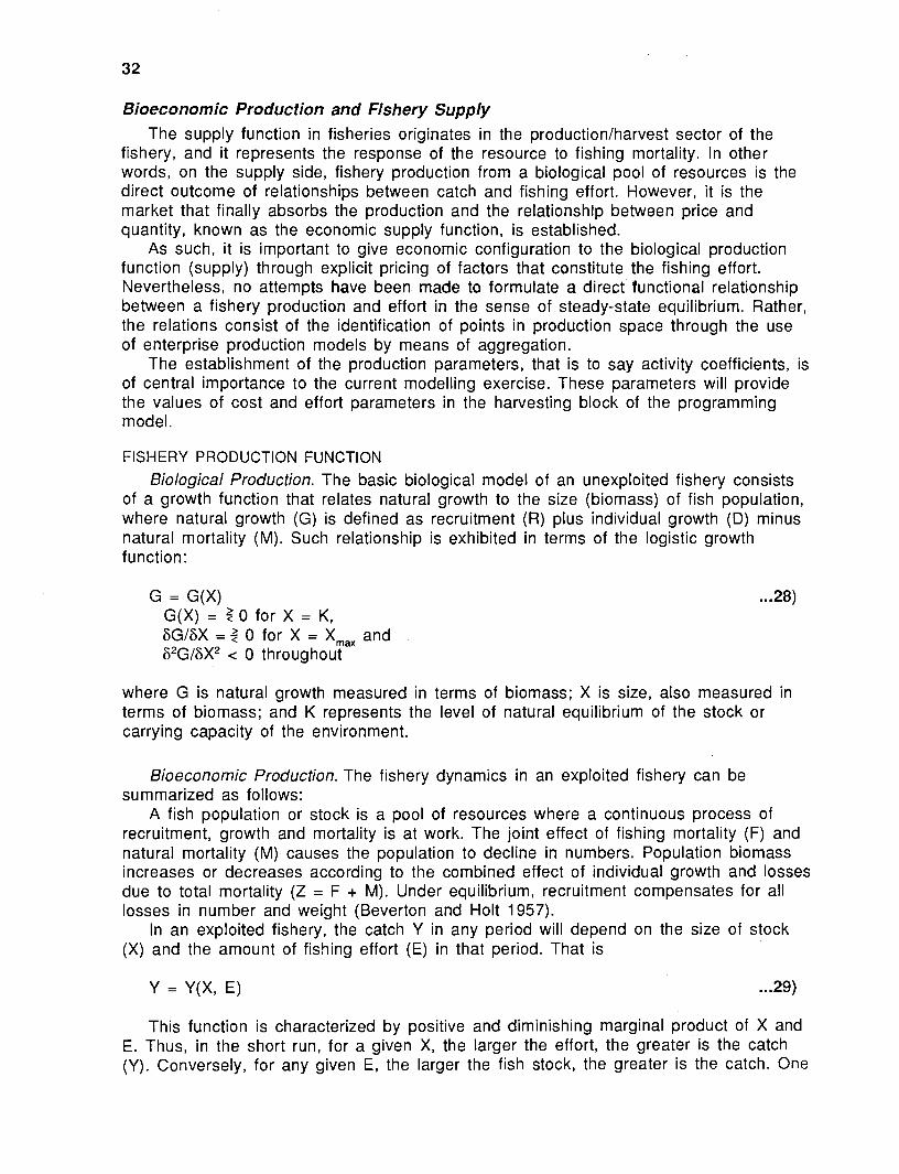
Bioeconomic Production and Fishery Supply The supply function in fisheries originates in the production/harvest sector of the
fishery, and it represents the response of the resource to fishing mortality. In other words, on the supply side, fishery production from a biological pool of resources is the direct outcome of relationships between catch and fishing effort. However, it is the market that finally absorbs the production and the relationshtp between price and quantity, known as the economic supply function, is established.
As such, it is important to give economic configuration to the biological production function (supply) through explicit pricing of factors that constitute the fishing effort. Nevertheless, no attempts have been made to formulate a direct functional relationship between a fishery production and effort in the sense of steady-state equilibrium. Rather, the relations consist of the identification of points in production space through the use of enterprise production models by means of aggregation.
The establishment of the production parameters, that is to say activity coefficients, is of central importance to the current modelling exercise. These parameters will provide the values of cost and effort parameters in the harvesting block of the programming model.
FISHERY PRODUCTION FUNCTION
Biological Production. The basic biological model of an unexploited fishery consists of a growth function that relates natural growth to the size (biomass) of fish population, where natural growth (G) is defined as recruitment (R) plus individual growth (D) minus natural mortality (M). Such relationship is exhibited in terms of the logistic growth function:
G = G(X) G(X) = 5 0 for X = K, 6G/6X = 3 0 for X = X,, and 62G/6X2 c 0 throughout
where G is natural growth measured in terms of biomass; X is size, also measured in terms of biomass; and K represents the level of natural equilibrium of the stock or carrying capacity of the environment.
Bioeconomic Production. The fishery dynamics in an exploited fishery can be summarized as follows:
A fish population or stock is a pool of resources where a continuous process of recruitment, growth and mortality is at work. The joint effect of fishing mortality (F) and natural mortality (M) causes the population to decline in numbers. Population biomass increases or decreases according to the combined effect of individual growth and losses due to total mortality (Z = F + M). Under equilibrium, recruitment compensates for all losses in number and weight (Beverton and Holt 1957).
In an exploited fishery, the catch Y in any period will depend on the size of stock (X) and the amount of fishing effort (E) in that period. That is
This function is characterized by positive and diminishing marginal product of X and E. Thus, in the short run, for a given X, the larger the effort, the greater is the catch (Y). Conversely, for any given E, the larger the fish stock, the greater is the catch. One

can have a family of short-run production (yield) curves, each defined for a particular population size. These are shown in Fig. 3.4, where the greater the population the greater will be the yield resulting from a given level of effort.
Combining equations (28) and (29) and setting Y = G, gives:
X* = @(E) 6@(E)/6E < 0 and 62@(E)/6E2 < 0
where X* is the population equilibrium size, i.e., the fish stock corresponding to a catch that is equal to natural growth (Y* = G). Equation (30) represents the population equilibrium curve (Panayotou 1985).
Substituting equation (30) in equation (29) gives the yield effort curve or the sustainable yield equation (31)
where Y* is sustainable yield in the sense that Y* = G and that corresponding fish stocks remain unaffected by fishing (as long as E remains constant).
The following properties hold for equation (31):
(a) 6 ~ * / 6 ~ > 0 for OcEcEmSy (b) 6 ~ * / 6 ~ = 0 for E=Em9 (c) GF*/FE < 0 for E'E,,,,
Any point on F*(E) gives a sustainable yield, i.e., a catch that is equal to natural growth of the corresponding fish stock, which can be maintained as long as effort remains unchanged.
The representation in equation (31) gives the long-run steady-state yield (production) function of a fishery. Although the fish stock size or resource abundance varies among fishing grounds and time periods (seasons), in the short run, under a defined seasonal context, the fish stock (X) in a particular fishery will be here assumed to be constant. This allows estimation of the production function of the simple form given in equation (32) .
where Y = catch and E = effort (index).
FISHING EFFORT AND ITS INTERNAL STRUCTURE
The concept of fishing effort occupies a central position in fisheries economics literature. This is due to the emphasis given by management regimes to regulate one or more of its components as management tools (Clark 1976; Anderson 1977; Scott 1979). The term fishing effort in equation (32) is a composite input, often broken down into its typical elements such as labor, capital, material and time spent. These elements can be further decomposed depending on the nature and the type of fishery. For example in small-scale and traditional nonmechanized fishing, it is boat and gear that make up the major capital, as opposed to engine, power block, refrigeration facilities and fishing aids along with vessel and gear that constitute the major elements of capital in large-scale industrial fishing.

The amounts of all the capital components mentioned above, plus labor (assuming a fixed crew size) determine the catching power of a fishing unit, whereas the time spent in fishing determines the rate of utilization of existing fishing capacity. If a variety of fishing gear is used, it may be necessary to classify fishing units by type of gear used, as they represent different fishing strategies and hence different catching power. For instance, the use of push nets, trawl nets, gillnets, seine nets, hooks and line etc., may all represent different catching power in the context of a particular fishery.
In fact, the operators of a fishing unit combine capital (K), labor (L), materials (M) and managerial skill (N) to produce catching power, which when multiplied by time (h) spent in fishing gives the total amount of effort expended. This gives:
The variable effort in equation (33) is typically part of an input combination process. Often, factors of production are combined to form a composite input index of effort, which becomes an input in the fishery production function (Anderson 1976; Squires 1987). However, direct estimation of the effort through use of specifications similar to equation (33) may not always be practical.
Production Models for the Riverine Fisheries of Bangladesh
IDENTIFICATION AND DEFINITION OF VARIABLES AND MODELS
The formulation of a production model for these fisheries requires the identification of the important variables that define fishing effort and subsequently determine yield. They include: (i) population size of different species and their periods of abundance; (ii) type of environment and their geo-physical features; (iii) type, size and other characteristics of boat and gear; (iv) the number of fishers, time spent in fishing and their skills; and (v) intensity of fishing over season (i.e., length of fishing periodlseason).
The major groups are hilsa, carp, catfish and prawns, constituting 62% of the average annual catch, hilsa alone being 44% (Table 2.2). Moreover, the distribution of these species seems to follow spatial and seasonal patterns as described earlier. Although groups other than the above do not individually constitute a separate fishery, their aggregate can do so. Fishers who catch these mixed species rather than the four major groups are found everywhere. As such, these species can be said to constitute a fifth fishery based on "miscellaneous species".
Although boat characteristics do not differ across fisheries except in size, the types of gear used and their size exhibit wide variation as stated in Chapter 2.
As regards fishing labor, its size and skill depend on the size of boat and gear and type of gear used. Usually fishers spend more hours in fishing during the peak months of harvest than in lean months. In addition, there are other factors that contribute to the harvesting process, such as floats and weights for keeping nets upright, sails of a boat, lanterns and flashlights, deck facilities, etc.
Given the above description on the variables defining effort and determining the resultant fish production from the in lwd open waters, a traditional functional relationship for each individual species i at time t can be shown by equation (34)
where i = species (group); t = time; Y = tonnage of harvest; S = fishing season; A = river andlor fishing ground); B = boat capacity; R = gear capacity; L = fishing crew; and 0 = other inputs (floats and weights, sail, lanterns, flashlights, etc.).

The variables on the right hand side of equation (34) can also serve as factors that define an effort index similar to that in equation (33).
SPECIFICATIONS OF THE ECONOMETRIC MODEL
In the absence of confirmed biological knowledge of the number and stock size of each species group and their distribution across water areas (or rivers) and over seasons, fluctuation as well as the spatial differences in both absolute and relative harvest of each group can serve as a basis for making seasonal and spatial distinctions. Thus, the production models are separated by seasons (dry and wet season) and rivers (four river groups). The separation of fisheries in terms of two seasons is consistent with the fishing calendar followed by both management authorities and fishers. The grouping of rivers in terms of three principal river systems and other small rivers is also consistent with the grouping followed by the Fisheries Resource Survey System (BFRSS) of the Department of Fisheries (DOF).
While fishing seasons (S) and rivers and/or fishing grounds (A) are distinguishable in the manner discussed above, variables B, R and 0 require further specification. Since the boats vary in length, width and draft, they all are considered as principal determinants of boat capacity (B). However, these parameters usually follow a definite proportion, and they might give rise to the problem of multi-collinearity when used as independent variables in an econometric estimation model. A single measure to represent boat capacity could be the total volume (length x width x draft) or tonnage. Khaled (1985) used tonnage of boat capacity and found it significant in estimating the production technology of hilsa fishing in the Meghna and Padma Rivers.
Similarly, capacity of a gear (G) depends on the type of gear (net type, hook or lines), length, depth and mesh size (in case of net) and number of hooks and their size (in the case of hooks and lines). Therefore, these parameters of gear should also be treated as determinants of production. However, mesh size of net is found to be typical for a particular target but varies over seasons where the size of fish caught is different. For instance, the size of hilsa caught during the dry season is smaller than that caught in the wet season. As such, mesh size would not be significant in explaining production differentials (Khaled 1985). On the other hand, to capture differences in net type, either dummy variables or a standard unit of gear can be used, while the size of net can be measured by the surface area (m2) of the net.
As for the other inputs (0), most (e.g., sail, floats and weights) are proportional either to the size of boat or to size of net. Hence they can be excluded from the function.
The catch quantity (Y) includes only that of the target species. Other species would be treated as by-catch obtained from the effort directed to the major species groups being modelled.
Thus, an econometric model for seasonally and spatially (riyers) distributed target groups can be further specified as
where i = groups (1,2,..,5); r = river (1,2,3,4); s = season (1,2); t = time (year); Y =
tonnage of production; B = tonnage of boat(s); R = surface area of net(s); L = size of crew; H = fishing time (hours); D = dummy variable for gear type; and U = error term.
The functional relation in equation (35) is a multiple-input production function. As such, effects of changes in the effort intensity on fishing mortality are only partially represented by changes in each of the individual factor inputs. A single relation of

production and effort, is therefore, more useful for explaining the fishery dynamics. As mentioned earlier, effort in equation (32) translated in terms of component factors in equation (33) is an index and, as such, gives a single measure of effort. However, the measurement of an index through equation (33) may give biased resuits if the relative weights of individual factors and their variants are arbitrary. The use of a single real economic factor that can serve as an indicator of fishing power as a measure of effort is more appropriate. Also, factor inputs both in equations (33) and (35) may follow a definite proportion in producing effort as well as output, thereby exhibiting a high correlation between each other.
Considering the above, fishing gear capacity (defined below) has been chosen as a measure of effort in the current framework. This variable appeared more relevant in defining the fishing power of an individual fishing unit as well as that of the fleet in the concerned fisheries, although it is the boat that normally defines a fishing unit and holds the fishing crew, gear (nets or hooks) and other material on-board while fishing. The Fisheries Resource Survey System initiated through the FAOIUNDP used gear as a unit of effort (Tsai and Ali 1985).
Usually, boat and crew size are weak indicators of fishing power in small-scale multispecies and multigear fisheries (Prof. H.C. Lampe, pers. comm.). The size of crew follows a proportionate relation to the size of gear in a particular fishery at a given time. That proportion can, however, change independently of gear size depending on the opportunity cost of labor and overall economic situation in the country.
Similarly, boats of a certain size-range are found to operate with a wide range of gear capacity. This is because gear is a less durable and more highly depreciable asset than a boat, and investment on gear depends on the financial strength of the individual fishing units. In essence, it is the size and capacity of gear (including the time spent in fishing) that makes a marked distinction between the fishing power of individual fishing units.
Given the gear capacity as the single explanatory variable determining the production, the input-output relationship in equation (35) reduces to a more useful yield- effort relationship similar to equation (32), this time with a unit measure of effort. However, rather than the total tonnage of harvest the dependent variable could as well be the catch per unit of effort (CPUE) shown in terms of equation (36).
CPUE = G(E) ... 36)
where CPUE = catch per unit of effort; and E = total fishing effort (gear capacity).
GEAR CAPACITY AND METHODS OF STANDARDIZATION Gear capacity is defined as:
G = S x T
where S = surface area of the net(s), = lengthlpiece x width (depth) x no. of pieces of net; and T = total fishing hours during the season, = total days of fishing x average fishing hours per day.
The above definition of gear capacity will not hold good for all types of gear used in a particular fishery. In standardizing the effort (gear capacity) of each species I have assigned the fishing gear that catches the major portion of the catch as the standard. The efforts of all other gear are expressed in terms of the dominant gear by dividing their gross catch by the average CPUE of the dominant gear (Tsai and Ali 1985).
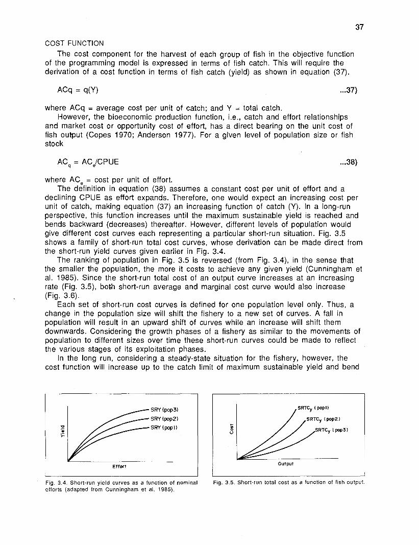
COST FUNCTION
The cost component for the harvest of each group of fish in the objective function of the programming model is expressed in terms of fish catch. This will require the derivation of a cost function in terms of fish catch (yield) as shown in equation (37).
where ACq = average cost per unit of catch; and Y = total catch. However, the bioeconomic production function, i.e., catch and effort relationships
and market cost or opportunity cost of effort, has a direct bearing on the unit cost of fish output (Copes 1970; Anderson 1977). For a given level of population size or fish stock
AC, = ACelCPUE ... 38)
where Ace = cost per unit of effort. The definition in equation (38) assumes a constant cost per unit of effort and a
declining CPUE as effort expands. Therefore, one would expect an increasing cost per unit of catch, making equation (37) an increasing function of catch (Y). In a long-run perspective, this function increases until the maximum sustainable yield is reached and bends backward (decreases) thereafter. However, different levels of population would give different cost curves each representing a particular short-run situation. Fig. 3.5 shows a family of short-run total cost curves, whose derivation can be made direct from the short-run yield curves given earlier in Fig. 3.4.
The ranking of population in Fig. 3.5 is reversed (from Fig. 3.4), in the sense that the smaller the population, the more it costs to achieve any given yield (Cunningham et al. 1985). Since the short-run total cost of an output curve increases at an increasing rate (Fig. 3.5), both short-run average and marginal cost curve would also increase (Fig. 3.6).
Each set of short-run cost curves is defined for one population level only. Thus, a change in the population size will shift the fishery to a new set of curves. A fall in population will result in an upward shift of curves while an increase will shift them downwards. Considering the growth phases of a fishery as similar to the movements of population to different sizes over time these short-run curves could be made to reflect the various stages of its exploitation phases.
In the long run, considering a steady-state situation for the fishery, however, the cost function will increase up to the catch limit of maximum sustainable yield and bend
SRY (pop3)
SRY (pop21
I! SRY (popl) .- t
Effort I Output
Fig. 3.4. Short-run yield curves as a function of nominal efforts (adapted from Cunningham et al. 1985).
Fig. 3.5. Short-run total cost as a function of fish output.
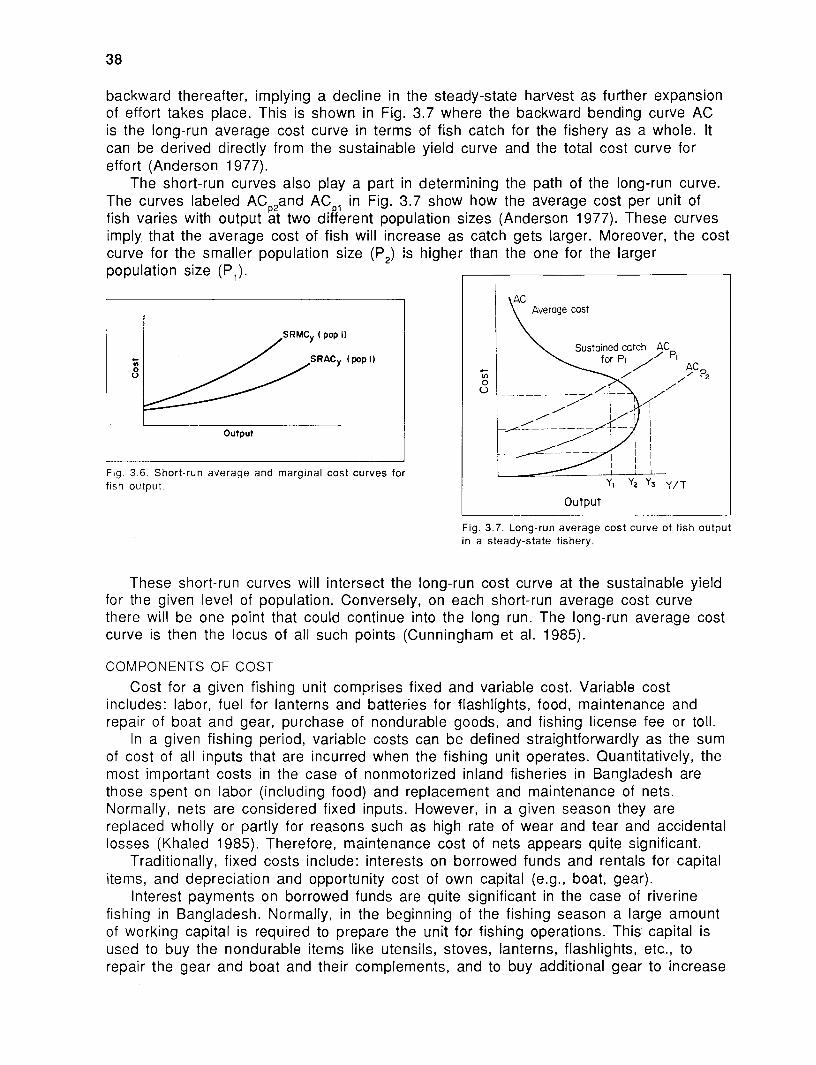
backward thereafter, implying a decline in the steady-state harvest as further expansion of effort takes place. This is shown in Fig. 3.7 where the backward bending curve AC is the long-run average cost curve in terms of fish catch for the fishery as a whole. It can be derived directly from the sustainable yield curve and the total cost curve for effort (Anderson 1977).
The short-run curves also play a part in determining the path of the long-run curve. The curves labeled ACp,and AC , in Fig. 3.7 show how the average cost per unit of fish varies with output at two difierent population sizes (Anderson 1977). These curves imply that the average cost of fish will increase as catch gets larger. Moreover, the cost curve for the smaller population size (P,) Is higher than the one for the larger population size (P,). r
Output
Fig. 3.6. Short-run average and marginal cost curves for fish output
Output
Fig. 3.7. Long-run average cost curve of fish output in a steady-state fishery.
These short-run curves will intersect the long-run cost curve at the sustainable yield for the given level of population. Conversely, on each short-run average cost curve there will be one point that could continue into the long run. The long-run average cost curve is then the locus of all such points (Cunningham et al. 1985).
COMPONENTS OF COST
Cost for a given fishing unit comprises fixed and variable cost. Variable cost includes: labor, fuel for lanterns and batteries for flashlights, food, maintenance and repair of boat and gear, purchase of nondurable goods, and fishing license fee or toll.
In a given fishing period, variable costs can be defined straightforwardly as the sum of cost of all inputs that are incurred when the fishing unit operates. Quantitatively, the most important costs in the case of nonmotorized inland fisheries in Bangladesh are those spent on labor (including food) and replacement and maintenance of nets. Normally, nets are considered fixed inputs. However, in a given season they are replaced wholly or partly for reasons such as high rate of wear and tear and accidental losses (Khaled 1985). Therefore, maintenance cost of nets appears quite significant.
Traditionally, fixed costs include: interests on borrowed funds and rentals for capital items, and depreciation and opportunity cost of own capital (e.g., boat, gear).
Interest payments on borrowed funds are quite significant in the case of riverine fishing in Bangladesh. Normally, in the beginning of the fishing season a large amount of working capital is required to prepare the unit for fishing operations. This capital is used to buy the nondurable items like utensils, stoves, lanterns, flashlights, etc., to repair the gear and boat and their complements, and to buy additional gear to increase

the fishing capacity of the unit. The source of such capital is from usury sources (private moneylenders or fish traders), and they usually charge a rate of interest ranging from 8 to 10% per month (BCAS 1987).
To calculate depreciation (d), the purchase price or capital cost (P,) of such fishing assets such as boats, anchors and nets, their economic life (L) and their scrap or salvage value (S) are needed.
However, calculation of depreciation for boats or nets is not important as a component of cost in the context of fishing. In fact, in fishing operations constant repair and maintenance keep the asset almost equally productive for a longer time than contemplated in the approach of depreciating the asset at a certain rate. Moreover, if proper repair and maintenance costs are included in the calculation of cost, inclusion of typical depreciation allowances may result in double counting.
Aside from these, there is a wide range of variations in the structure of fishing costs, delivered through several channels; modes of payment for each of them vary across fishing unit and fishing ground. Important among them are labor and capital items. In terms of the previous definition of cost, labor cost is treated as a variable cost. This assumes a fixed wage rate, similar to that of hired labor in agriculture. However, in practice, it is common for the crew to be paid a share of the value of catch instead of the fixed wage rate. In addition, among individual crew members, payment or share varies according to skill and role in the fishing process. This procedure applies to owner's labor also, and thus makes such cost a real one.
Similarly, if capital items such as boat and gear are rented by the fishing unit, payment is made most of the time in terms of a share of catch, instead of cash rents. This is a common practice when the crew members provide some of the capital items to be used by the fishing units.
The Market Submodel
A quantitative analysis of demand-supply and price relationships of different species of fish is necessary to provide an appropriate price mechanism in the programming model. The parameters of econometrically estimated functions are required as inputs into the programming model to determine solutions to the market model simultaneously with the other submodels (technological and biological).
The price analysis will provide two important informations: (i) specific economic coefficients (parameters) such as price and income elasticities (or flexibilities) of demand (or prices); and (ii) forecasts of prices or variables affecting prices.
The model was conceived at three levels, i.e., ex-vessel, wholesale and retail markets between the fishers and the consumers in terms of important determinants, although the model for wholesale market could not be estimated because of lack of data. Effort was made to isolate and demonstrate spatial differences and seasonal changes in the demand for each of the fish species, especially at the ex-vessel level. The model contains equations wherein the functional relations of the major determinants of supply and demand are postulated.
EX-VESSEL MARKET
The ex-vessel market refers to the market where fishers deal with the first buyers. The buyers are mostly assemblers or collectors. The process of collecting is confined to the area comprising the fishing grounds up to assembly points or landing sites. A large number of nonmotorized (a few motorized) boats are engaged in collecting fish from the small fishing units scattered over the fishing grounds in the riverine waters in different

regions of the country. The conduct at this level is rather simple. Harvested fish are channelled to the assembly point by a group of middlemen (agents) whose numbers are more or less limited, having some informal agreement with the harvesters with regard to the transaction.
Variables that reflect behavior of price in this market are: the level of harvest, their size and quality, the fishing ground, cost of transportation, existence of landing stations and their proximity to the fishing grounds, weather conditions affecting harvesting activity and seasonal abundance of harvest.
Although markets are separated between locality or area of fishing and hence prices of individual fish species in each market would differ, the free flow of information among markets can easily act against marked price differential among small local ex- vessel markets.
The existence of a strong seasonality in the abundance and availability of various groups of fish in different fishing grounds would also influence the pricing of fish in each market. This might give rise to separate seasonal markets at the ex-vessel level reflecting seasonal differences.
Distinction between markets can also be made by region as there are important differences in the availability and abundance of species in each region as well as final demand conditions.
Another factor that could affect the pricing mechanism is the market power of buyers (collectors) and sellers that determine the degree of competition in each individual market. At the ex-vessel market buyers are able to exert some extra- economic power on the sellers because of credit ties, the buyers being the suppliers of capital for fishing to the sellers (fishers). The existence of such force could possibly distort the competitive pricing process. However, as the numbers of buyers and sellers become large and there is better flow of information between markets, the distorting forces become weaker. The same is true in the long-run, whereby forces of competition would correct such distortions.
Also, if the flow of information on prices and harvest is perfect, the prices prevailing in other areas affect the price in a particular market and vice versa. The distance between the area of fishing and the landing center also affects the price through its effects on communication means, transport cost, postharvest handling and freshness. However, if the flow of information is perfect and complete among markets, other things remaining the same, the prices in each market will only differ by the extent of transport costs.
Since the demand at the ex-vessel market is derived from the upper markets (wholesale and retail), the prices in the upper markets, especially the wholesale price, directly influence the price in the ex-vessel market.
On the demand side, a particular ex-vessel market price at any point in time (t) would generally depend on the landings. As stated earlier, the production (supply side of the fishery) being dependent upon various exogenous factors, it is the quantity demanded that determines the price, at least in the short run. As such it is more logical to conceive the demand in terms of price (Farrell and Lampe 1965; Waugh and Norton 1969; Wang 1976; Bockstael 1977; Storey and Willis 1978; DeVoretz 1982; Wang et al. 1978, 1986; Cook and Copes 1987).
Thus, separating markets by species, locality, landing center, fisheries region and seasons of fishing we can state the ex-vessel demand prices (Pvd)as:

where i = species j = locality/ area of fishing k = landings market I = fisheries region m = season of fishing t = time period (a month) Qi = landing quantities of the species Si = size (or weight) of landed species Po,x = composite prices of other species P,,,,, = average price of species (i) in the upper (wholesale) market(s).
The supply side of the market for fish at the ex-vessel level needs special explanation. Unlike many other industrial and agricultural commodities, the supply of fish in the short run is governed more by biological, environmental and technological factors than by price. Such factors are dominant in the short and medium run. Moreover, fish are usually marketed fresh. As such, the important determinant of supply is the current rate of fishing mortality and past history of mortality rates, which in turn are determined by the aggregate level of effort devoted to fishing and also on catchability coefficient (Lampe 1967). If the level of fishing does not change (which is likely in the short run), the supply is predetermined by natural factors in a particular ex-vessel market.
In the long run, however, supply (harvest) of a fish species will be affected by its price, prices of other species, prices or opportunity cost of inputs (effort) and productivity of inputs (amount of effort per unit of output).
The ex-vessel supply (QvS) of a particular species (i), in a particular local ex-vessel market (j), within a landing center (k), region of fishing (I), season (m) and at time period (t) can, therefore, be regarded as predetermined as shown in equation (40).
where 'A' is a predetermined value of landings of species (i), which is the outcome of several exogenous natural and physical factors. Hence, the supply price is perfectly flexible with respect to given quantities of ex-vessel landings.
The above formulation assumes separate markets for each locality or area of fishing. As such, markets are considered relatively thin and are confined to a limited number of buyers and sellers who are isolated from their counterparts in other areas. However, if one considers the free flow of information on price, landings of species and other variables affecting price relations, these small markets could be aggregated into one single market over a region or at least over a landing center for wholesale trading. This generalization appears more realistic as discussed in the next section (section on wholesale market) in that the market operating between the fishers and assemblers/ collectors is part of the same market based in the landing centers or docksides. In fact, the collectors/ assemblers are in most cases the commission agents or buying agents of the fish traders based in the landing centers or dockside markets (FAO/Rapport 1986).
Based on the above generalization the specification of demand and supply model within the regions can be simplified.
WHOLESALE MARKET
At this level demand is broad with alternatives available. Moreover, the market is stretched in a long chain (vertical and horizontal) of intermediaries spread all over the region/country dealing with the fish before it goes to the retail market.

The chain of marketing immediately after the first level of wholesale (sale by the assemblers or collectors) is complex, involving movement across regional boundaries and changes of intermediaries and dealers. Therefore, the number of variables that enters into the market clearing process can be quite large depending on the stage of wholesale in the marketing chain in the course of horizontal and vertical movement of fish. Important among them are: prices (including other species), net amount of fish available for wholesale (including other species), regional location of fishing and markets, distance between assembly point and wholesale market, type and extent of postharvest handling operations, means of transport and its cost, regional preference for the species, prices in the retail market and seasonality.
Although markets at the wholesale levels consist of two submarkets and several intermediate stages performing marketing functions they can be simplified into one level by treating the first level wholesale market (i.e., the transaction between collectors or assemblers as part of the ex-vessel market and subsuming the other intermediate market levels into the final wholesale market (urban or suburban wholesale markets) along the chain as transportation and commission service activities.
Even though supply at the ex-vessel level is predetermined, at the wholesale level it would be considerably affected by price, as the amount of fish inflows and outflows to and from each region will respond to price movements. The net flow (regional import - regional export) will be a function of price. Therefore, at the wholesale level the net supply quantity (which is different from landing quantities) will become a determinant of price or vice versa.
Given the above simplifications the wholesale price equations for demand (Pwd) and quantity equations for supply (QwS) for a species (i), in region (I) and season (m) can be represented by equations (41) and (42).
where i = species I = region m = season of fishing t = time period (a month) Qwi = quantities of the species (i) demanded Si = size of species (i) Pwx = composite prices of other species -Pri = price of species (i) in the upper (retail) market Np = size of population
where i = species I = region m = season of fishing t = time period (a month) Q,, = Q[(landings) + M(import) - F(export)] Pwi = price of species (i) Pwx = composite prices of other species (x)
Pri = price of species in the upper (retail) market PwZ = wholesale price of species (i) in other regions.

RETAIL MARKET
This market represents the primary demand (consumer demand) from which demands in the lower markets are derived. Transactions take place between retailers and consumers. At this level variables that are important determinants of supply- demand and price relationships are quantities and prices of fish and other substitute goods, income, population and taste. However, since individual retail markets are scattered and have considerable difference in terms of transport and communication as well as purchasing power of the consumers (e.g., urban and rural), distinct independent local or regional retail markets can exist.
In functional form the price equation for demand (Prd) and quantity equation for supply (QrS) at the retail level can be represented in terms of equations (43) and (44), respectively.
where i = species I = region m = season of fishing t = time period (a month) Qr, = quantities of the species (i) demanded in the retail market S, = size of species (i) Prx = composite prices of other species Pa = prices of substitute animal proteins Np = size of population served by the retail market In = personal income of consumer Cf, = consumer preference for fish (i)
where i = species I = region m = season of fishing t = time period (a month) Pr = price in the retail market Prx = price of other species Pa = price of other animal proteins
SPECIFICATION OF THE ECONOMETRIC MODEL
In the definition of general economic relationships in the previous sections we have seen that the role of price (demand) is more important in the market model, at least in the ex-vessel market. Moreover, in a market where supply is predetermined at a given time 't', it is the variable 'P' (price) that is required to be determined. The quantities can at best be assumed to be determined recursively, i.e., supply is determined by past prices (Tomek and Robinson 1981). Keeping this in view, the interest in the following sections will be to specify the demand equations for econometric estimation.

MARKET DEMAND EQUATIONS
In our demand model price is the logical dependent variable, while quantity of fish as well as prices and/or quantities of other substitute goods are specified as independent variables. There are other independent variables that will also be used in the model as important explanatory variables in estimating demand equations for different market levels. Moreover, since one of the objectives of the model building is to simulate price movements, it is quite logical to treat prices as a dependent variable (Waugh 1964; Tomek and Robinson 1981). Two recent studies by Wang et al. (1986) and Cook and Copes (1987) followed similar specifications, consistent with previously cited fishery economic models, e.g., Farrell and Lampe (1965), Waugh and Norton (1 969), Bockstael (1 977) and DeVoretz (1 982).
AGGREGATION OF SUBMARKETS
Some of the submarkets at various market levels, defined earlier, can be aggregated into a single market with regard to the formulation of empirical function expressing the demand equations at various market levels. Such aggregation has been applied over space, species of fish and time.
Spatial aggregation. The specification of demand function for ex-vessel market within the space of the region will bring all scattered local markets and landing centers within one region under the influence of the same market forces and other exogenous factors. Such simplification is logical considering the fact that ex-vessel prices generated at the landing markets are based upon the flow of information and competition among buyers and sellers in regional, ex-vessel, and wholesale markets. The Padma-Meghna and Brahmaputra river system divides the whole country into four separate geographic regions. These four regions are quite distinct in terms of availability of fisheries resources, means of transport and communications. On this basis, therefore, we aggregated the small and segregated markets into four regional markets comprising the regions defined as SE (southeast), SW (southwest), NE (northeast) and NW (northwest) parts of the country. In the empirical models three instead of four regions have been distinguished by combining the southeast (SE) and northeast (NE) regions into a single region. However, at the retail level the aggregation will be broadened to reduce the regions into a single retail market.
Species aggregation. There are many varieties of species of fish captured from the rivers. However, not all of them are important in terms of ability to form a separate market. In fact, a great many of them are similar biologically and ecologically and/or have similar preference among buyers in terms of price and tastes.
The model considers six separate species markets, one each for four major species, i.e., hilsa, carp, catfish and prawn. The fifth market includes the remaining categories of fish (miscellaneous fishes) harvested from the open waters. The sixth market is considered for large prawns, since a sizeable quantity of large prawns are exported.
Temporal aggregation. Given the pattern of periodicity in the catch rates of different species of fish, two distinct seasonal markets (wet and dry season) have been distinguished for each species, which are quite consistent with the fishing calendar followed by small-scale riverine fishing. Based on the above, the monthly markets have been aggregated into two different seasonal markets. The months covered under each season are: April-September for the wet season and October-March for the dry season.
FUNCTIONAL FORM AND CHOICE OF VARIABLES
In selecting the functional form, simplicity was considered as one of the important criteria, although care was exercised to conform to the criteria of mathematical

properties of functions and statistical tests. We defined the demand functions at various levels in terms of equations (45) to (47).
where i = species (1, 2, ..., 5) I = region (1, 2, 3) m = season (1, 2) t = monthlyear Pv, = ex-vessel price of species (i) Pw, = wholesale price of species (i) Pr, = retail price of species (i) Qv, = landed quantity of species (i) Qw, = net wholesale quantity traded in the region
= Qv, + Mi - Fi = landed quantity + regional import - regional export
Qr, = retail quantity of species (i) Pvx = ex-vessel price of other species Pwx= wholesale price of other species Pr, = retail price of other species or substitute products Pv, = ex-vessel price of species (i) Pwi = price of species (i) in the wholesale market Pr, = price of species (i) in the retail market Np = populaton size In = personal income Si = size of fish caught.
Price Differences Between Market Levels and Postharvest Cost
A relationship between demand functions at various market levels (equations (45) to (47)) can now be established in terms of marketing margins, defined as the difference between primary and derived demand curves for a particular fishlfish products (Tomek and Robinson 1981). In such a case, retail demand function representing the primary demand is determined by the response of the ultimate consumer, while the ex-vessel and wholesale demand functions are derived demand functions determined by the price quantity relationship which exists at the ex-vessel level or an intermediate point where fish is purchased by wholesalers or processors. Thus, given several simplifying assumptions, the derived demand for fish at the ex-vessel and/or wholesale levels is obtained by subtracting the per unit costs (prices) of all the marketing and processing components from the primary demand functions. Fig. 3.8 shows demand curves at two market levels (ex-vessel and retail), assuming a perfectly elastic supply functions for marketing services (Tomek and Robinson 1981).
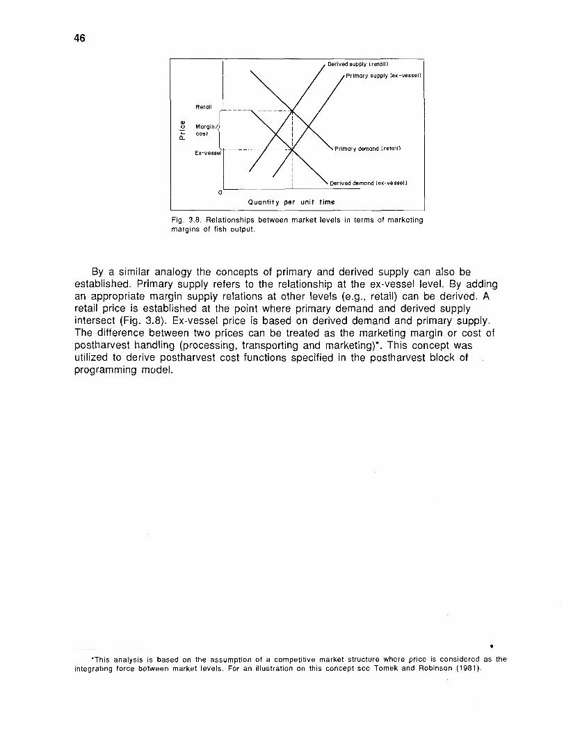
Derived supply (retall)
Primary supply (ex-vessel)
Primary demand (retail) Ex-vessel
Derived demand (ex-vessel
0
I Quantity per unit time
Fig. 3.8. Relationships between market levels in terms of marketing margins of fish output.
By a similar analogy the concepts of primary and derived supply can also be established. Primary supply refers to the relationship at the ex-vessel level. By adding an appropriate margin supply relations at other levels (e.g., retail) can be derived. A retail price is established at the point where primary demand and derived supply intersect (Fig. 3.8). Ex-vessel price is based on derived demand and primary supply. The difference between two prices can be treated as the marketing margin or cost of postharvest handling (processing, transporting and marketing)*. This concept was utilized to derive postharvest cost functions specified in the postharvest block of programming model.
'This analysis is based on the assumption of a competitive market structure where price is considered as the integrating force between market levels. For an illustration on this concept see Tomek and Robinson (1981).

CHAPTER 4 PARAMETER ESTIMATION: BlOECONOMlC AND MARKET SUBMODELS
Bioeconomic Submodel
Production and Cost Equations
Since the programming model is cast in a long-run framework, the cost coefficients must be derived from a long-run production function. Unfortunately, precise estimates for a long-run production function (yield function) are impossible at this stage as time series of catch and effort on each of these fisheries (either separate or in aggregate) are not available. Instead, a short-run relationship of yield and effort [equation (36)] was used, and subsequently the relationship of cost and yield shown in equation (37) was established for the current level of population through modelling individual fishing enterprises for each of the five species of fish mentioned earlier.
Also, the models for each species were separated by season (two seasons) and river groups (four groups). While separate equations were estimated for individual species in each season, dummy variables were used to capture structural differences in cost and production between the enterprises operating in different river groups. Equation (48) shows the structure of the cost function finaliy chosen for econometric estimation.
where i = species (1,2,..,5); I = season (1,2); Q= quantity of catch in weight; Dk= dummy variables for river groups (D,,D,,D,).
Given the short-run yield and cost curves for a given population size, the movement of the fishery with varying population sizes could be traced with the help of catchability coefficients, defined as the fraction of total stock removed by each unit of effort, assumed to be constant for each level of population size in the different fisheries. In such a case, a catchability coefficient for a fishery at any given level of population size will be proportional to the CPUE.
In determining such coefficients the relative fish population/stock size in different fisheries at current times in terms of density or current catch levels can be used. The values of current catchability coefficients in different fisheries will indicate the relative status of each fishery and the movement of long-run yield and cost functions as the population/stock size moves towards low to high or vice versa.
The movement of production traced through the procedure described above may not yield the true function through which each individual long-run production would move. However, in a sectoral framework, where effort allocation among fisheries follows interdependencies, identification of relative positions will suffice the need of the true function for analysis of policies and management issues.

Data Data were obtained from a cross-sectional survey of fishing units operating in the
rivers. The samples include fishing units operating in the three main river systems (Meghna, Padma and Jamuna-Brahmaputra) and three small rivers representing other river groups in the present modelling framework. In selecting the sample we used the Fisheries Department's survey of fishing village and fishing boats as the main reference (DOFIBFRSS 1982). The number of fishing boats recorded in this survey was roughly proportional to the estimated number of fishing units operating in different rivers (Table 34 - Appendix A). Based on the fishing village and fishing boat survey information, 12 areas in nine different districts covering the four river groups (Table 35 - Appendix A) were identified. The district(s) chosen for each river group were those constituting the largest fraction of total area under the river group (Table 33 - Appendix A).
The survey areas were selected on the criterion of large concentrations of fishing households to minimize cost and time and to obtain adequate samples from each area. A total of 415 samples were randomly selected (Table 35 - Appendix A) from among the list of fisherslfishing units available with the local fisheries officers (in most cases only a partial list was available).
The sampling design (Table 36 - Appendix A) showed only the distribution of fishing units by river grol;p and season. Selection of sample fishing units by target species was not possible due to a lack of information in the sampling frame on the target species of ihe fishing unit. Data on input-output and costs were obtained for each fishing season by administering a structured questionnaire (Appendix B). The period covered was the 1987-88 fishing year (April-March) separated into the two seasons - wet season (April - September) and dry season (October - March).
Some important procedures followed in obtaining the data are as follows: input- output and cost data were obtained on a daily basis since the fishers customarily keep records and/or recall expenses for their day's fishing operation. Seasonal figures were obtained through multiplying by the total number of fishing days per season. In calculating the effort and cost per unit of effort only output of the direct (target) species group was considered. Catches of other species were considered incidental and treated as by-catch that augments income from fishing.
The raw data were processed using the statistical package SPSSPC*.
Estimation and Results The estimation of regression equations followed the usual ordinary least squares
(OLS). A linear functional form was fitted for equation (48). However, the dependent variable ACq was first computed using the formula in equation (38) before applying the OLS.
Although in each season models for each species in each river group were treated as separate, while performing the estimation a single regression was performed for all river groups, keeping only seasonal models separate (see specifications in equation (48)). However, dummy variables were used to distinguish one river group from the others in terms of production and cost structure in the cases of hilsa, carp, catfish and miscellaneous fish. For prawn, a single regression was performed combining datasets of all four river groups and two seasons. Two sets of dummy variables were used to represent differences due to season and river groups. This was done to have a larger sample size and thereby gain more degrees of freedom.
Table 4.1 shows the estimated average cost (ACq) equations for different species of fish in the rivers. As seen in Table 4.1, the 'F' values of AC equations for all the fisheries are significant. For hilsa and miscellaneous species fisheries, for instance, the
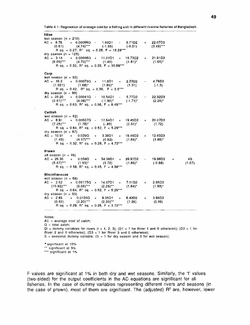
Table 4.1. Regression of average cost for a fishing unit in different riverine fisheries of Bangladesh.
Hilsa wet season (n = 210) AC = 8.78 + 0.00086Q - 1.60D1 - 3.71D2
(0.61) (4.74)"' (-1.55) (-0.31) R sq. = 0.27, R* sq. = 0.25. F = 13.28"'
dry season (n = 125) AC = 3.14 + 0.00056Q + 11.01D1 + 15.73D2
(8.05)"' (4.70)"' (1.40) (1.81). R sq. = 0.32, R* sq. = 0.29, F = 10.89"'
Carp wet season (n = 50) AC = 16.2 + 0.000750 + 1 l .8D l + 2.2302
(1.021) (1.68)' (1.85)' (1.31) R sq. = 0.42, R'sq. = 0.38, F = 5.5***
dry season (n = 80) A C = 2 8 . 2 0 + 0.00041Q - 10.54D1 - 5.77D2
(2.51)"' (4.06)"' (- 1 .go)* (-1.71). R sq. = 0.63, R' sq. = 0.56, F = 8.49"'
Catfish wet season (n = 62) A C = 8.91 + 0.00027Q - 17.64Dl + 19.45D2
(7.25)"' (1.78)' (-.85) (2.31)' R sq. = 0.64, R* sq. = 0.52, F = 5.29"'
dry season (n = 87) AC = 10.91 + 0.029Q + 3.38D1 + 19.45D2
(1.45) (4.1 7)'- (0.92) (1.66)' R sq. = 0.32, R* sq. = 0.28, F = 4.72"'
Prawn all season (n = 45) AC = 26.36 + 0.034Q + 34.38Dl + 39.97D2
(5.47)*** (1.93)* (1.72) (1 .86)* R sq. = 0.58, R* sq. = 0.45, F = 4.38"'
Miscellaneous wet season (n = 68) AC = 2.62 + 0.001 75Q + 14.07Dl + 7.01 D2
(1 0.92)"' (9.06)"' (2.26)" (1.84)' R sq. = 0.64, R* sq. = 0.52, F = 5.29"'
dry season (n = 93) AC = 2.83 + 0.0126Q + 9.95D1 + 6.42D2
(0.82) (2.20)'"' (2.30)** (1.26) R sq. = 0.29, R' sq. = 0.26, F = 3.72"'
Notes: AC = average cost of catch; Q = total catch; Di = dummy variables for rivers (i = 1, 2, 3); ( D l = 1 for River 1 and 0 otherwise); (D2 = 1 for River 2 and 0 otherwise); (D3 = 1 for River 3 and 0 otherwise); S = seasonal dummy variable; (S = 1 for dry season and 0 for wet season);
significant at looh " significant at 5% "' significant at 1%
F values are significant at 1% in both dry and wet seasons. Similarly, the 't' values (two-sided) for the output coefficients in the AC equations are significant for all fisheries. In the case of dummy variables representing different rivers and seasons (in the case of prawn), most of them are significant. The (adjusted) R2 are, however, lower

than 0.50 in most cases. The lowest R2 is observed for the miscellaneous species fishery in the dry season (0.26).
The AC equations for each fishery in Table 4.1 can be separated by river groups and seasons. Table 4.2 shows AC equations for the hilsa fishery separated by river groups in each season. The AC equations for other fisheries are shown in Table 37 - Appendix A.
Again, assuming that the cost parameters for the micro firms correspond to those for the entire fishery, the aggregate AC functions can be derived from the micro functions shown in Table 4.2 and Table 37 - Appendix A. The aggregate AC equations for each species separated by river group in each season are shown in Table 38 - Appendix A. Notice that the intercepts of the aggregate AC equations are the same as those of the corresponding sample AC equations, while only the slopes are different. In deriving the slope of the aggregate AC equations the aggregate average catch per season for the entire fishery has been substituted into the sample AC equation at the average catch rate for the sample, using the formula given below:
where C* = slope of aggregate AC equation; c* = slope of sample AC equation; q- = average catch rate for the sample; Q- = average catch rate for the fishery.
The aggregate AC functions for hilsa fishery are shown in Table 4.3.
Table 4.2. Computed average cost equations for a hilsa fishing unit in various seasons in the riverine fisheries of Bangladesh.
River group Equations
River 1 -dry season AC = 11.62 + 0.00056q -wet season AC = 7.185+ 0.00086q
River 2 -dryseason AC =18.87+0.00056q -wet season AC = 5.075+ 0.00086q
River 3 -dry season AC = 25.05 + 0.00056q -wet season AC = 30.85 + 0.00086q
River 4 -dry season AC = 3.14 + 0.00056q -wet season AC = 8.78 + 0.00086q
Table 4.3. Aggregate average cost equations for hilsa fishery in various seasons in the riverine fisheries of Bangladesh.
River group Aggregate AC equations
River 1 -dry season AC = 11.62 + 0.0002890 -wet season AC = 7.185+ 0.00021Q
River 2 -dry season AC = 18.87 + 0.00285Q -wet season AC = 5.075+ 0.00312Q
River 3 -dry season AC = 25.05 + 0.00225Q -wet season AC = 30.85 + 0.0035Q
River 4 -dry season AC = 3.14 ; 0.00057Q -wet season AC = 8.78 + 0.00029Q
- - ~ - - ~
Source: Based on estimated regression equations for sample fishing units. Notes: AC = average cost (BDT); q = catch (kg).
Source: Computed at the average rate of catch per season and based on equations in Table 4.2. Notes: AC = average cost (BDT); Q = catch ('000 kg).

Market Submodel
Market Demand Equations and Data In estimating the market demand models with the use of the specified choices of
variables in equations (45) to (47) an initial problem of data availability was encountered. First the complete absence of series and wholesale prices of different species of fish led to the dropping of the wholesale demand function from estimation. Price-quantity data on ex-vessel and retail levels were available only as monthly series for the period covering July 1983 - September 1987 mainly from published and unpublished records of the Bangladesh Fisheries Resource Survey System (BFRSS) in the Department of Fisheries and the published Monthly Statistical Bulletin of Bangladesh Bureau of Statistics (BBS 1984, 1985, 1986). The Department of Fisheries has available districtwise monthly records of ex-vessel landed quantities of fish from rivers by major species and their values. The Bangladesh Bureau of Statistics publishes monthly retail prices of important species of fish in selected districts. Monthly estimates of both ex- vessel and retail demand models were made based on districts.
With the time-frame of demand estimates being reduced to months, the use of size of population as a possible explanatory variable became less important, while the personal income data by month were unavailable from published statistical sources.
Since prices are nominal prices they have been deflated by the index of monthly consumer food price index (CPI) in the absence of an index of inflation. In a similar manner, catch quantities have been deseasonalized using a seasonal index in estimating retail demand equations.
Considering the data limitations and the above qualifications, retail and ex-vessel demand models were estimated for the six species groups.
For retail demand, a single market was assumed for each species (equation (50)). The variable list includes price of the species to be modelled as the dependent variable and its quantity and prices of all other groups as well as prices of chicken and beef as independent variables. The provision for a structurally different market between wet and dry seasons has been kept in the model through the inclusion of a dummy variable as one of the explanatory variables. In the case of big prawn the prices depend exogenously on the international market price. As such, their domestic retail price has been assumed to correspond to the export price and hence dropped from estimation in terms of a structural equation.
Significant structural differences over geographic regions and fishing seasons were explicitly considered in the case of the ex-vessel market [equation (51)l. Three regions (A, B and C) were defined for the ex-vessel market for each species. Catch quantities in Region A include the harvest from other rivers in the southeast and northeast Bangladesh and the Upper Meghna River; in Region B harvests include those from the lower Meghna River, Lower Padma River and other rivers in the southwestern part of Bangladesh; and in Region C they include the harvest from the Upper Padma River, Jamuna-Brahmaputra River and other rivers in northwestern Bangladesh. While separate functions were estimated for each region, seasonal differences in the price relations were explained with the help of a dummy variable. However, in the case of large prawns, only one ex-vessel market was assumed.
In the ex-vessel market model for a species in a particular region the variables included as explanatory variaMes were the region's ex-vessel quantity of the modelled species groups, ex-vessel prices of other groups in the region, ex-vessel prices of the various species groups in other regions, and retail prices of other species groups and other products. To model ex-vessel market for large prawns, their export price in the

international market was considered most important in addition to its ex-vessel price. However, in the absence of a time series on export price, FOB (freight on board) values of prawn and shrimp were used as a proxy variable.
Retail market: Pi = F(Q,, Pwi) ... 50)
where
Pi = retail prices of fish and other animal proteins;
Qi = retail quantity of ith species;
P-, = retail prices of cross products (fish and other animal protein; Px = ex-vessel price of ith species in jth region; Qx = ex-vessel quantity of ith species in the jth region; Px- = ex-vessel prices of other species in jth region; Px. = ex-vessel prices of all species in other regions; D = dummy variable;
= 1 for dry months: October-March = 0 for wet months: April-September
i = fish and animal protein (1, 2, .., 8) 1 = hilsa, 2 = carp, 3 = catfish, 4 = small prawns, 5 = miscellaneous fish, 6= beef, 7 = chicken, 8 = large prawns
j = region (1, 2, 3) 1 = Region A, 2 = Region B, 3 = Region C.
Data Evaluation The statistical characteristics of the raw data and their transformed version may give
rise to some potential biases and distortions open for questions and challenges. Some of the transformations and the potential biases in the data are discussed below:
First, the retail quantity data were the monthly amount produced - not consumed. Inventory adjustments, reductions due to postharvest processing and spoilage of production during postharvest handling in the course of marketing in the final retail market were not considered to correct for any difference in production and consumption. However, the resulting biases would still be considered minimum given the fact that most of the fishes harvested from the riverine environment are consumed fresh without much processing and product transformations.
Second, the quantity measures for each species were not ideal. They assume homogeneity within each fish species since quantity is defined in tonnes. Clearly, different sizes of fish that led to price differentials were not captured in the ex-vessel quantity and its value. Gates (1974) and DeVoretz (1982) cast serious doubt on such measures of quantity, and the former (Gates) opines that the same levels of landings in weight terms are associated with two equilibrium prices: one price for large fish and a lower price for small fish.
Third, the choice of substitute price for each species was arbitrary in the absence of a predetermined criterion. However, with respect to other substitute fish an arbitrary choice will not result in significant bias since consumers are largely indifferent in their preference and choice of fish. But the same may not be true with respect to choice between beef and poultry as substitute for each species. Fortunately, the price of beef has a direct bearing with imported livestock through informal trade in addition to

domestic beef production. This phenomenon might have introduced a bias in the price of beef and hence its inclusion as an explanatory variable might give less useful results. Considering this fact, and the presence of a high correlation between the beef price and poultry price we used poultry price as one of the explanatory variables in the final specification of retail demand models that were used for estimation.
Fourth, all prices, retail as well as ex-vessel, were deflated by the CPI. The biases resulting from such computation are also expected to be minimal.
Finally, the absence of an income variable in the model will introduce a bias in the estimates of flexibility (elasticity) coefficients for both own and cross prices, and, therefore, make the model less powerful for price (demand) forecasts.
Since the models are multivariate in nature they were a significant source of multicollinearity, one of the frequently encountered problems in econometric estimation of statistical models with multiple explanatory variables. Under this circumstance only a few among the listed variables in equations (50) and (51) were used in the final estimation keeping in mind the goodness of fit, level of significance of the model and its parameter estimates including the signs in each case. The rest of the variables were dropped from the specification of the models.
Similarly, the seasonal dummy variable 'Dl was also dropped from the specifications of those models where it appeared least important and/or became an additional source of multi-collinearity as well as distortion of expected signs, and a loss of goodness of fit and significance of the key variable (quantity) and the model itself.
Estimation and Results
The model has been cast as a single equation price dependent and supply independent. Therefore, the OLS method was chosen to fit a natural linear functional form and estimated. The natural linear functional form was estimated consistent with the main objective of its formulation, i.e., to provide an appropriate price mechanism in the programming model that can handle only linear demand specifications. The use of single equation model with OLS technique was found to be more practical in a number of instances and hence, it has been used and advocated by some authors, e.g., Labys (1 973), Wang (1976), DeVoretz (1982), Wang et al. (1986) and Cook and Copes (1 987).
It should be mentioned here that DeVoretz (1982) made a comparison between the parameter estimates of single equation price-dependent models and those of single equation quantity dependent and simultaneous equation models. His findings show that price dependent models are superior to their counterpart (quantity-dependent models). Also, between the OLS estimates of a price-dependent model and two SLS (two stage least square) estimates of simultaneous equation model, the former was found to yield best fit with little associated time series problems, whereas the latter yielded poor overall fit with some variables with either wrong sign or being insignificant.
The problem of autocorrelation and moving average errors also became significant for certain specifications. Under such circumstances attempts were made to correct them through a respecification. However, since such problems became unavoidable the familiar Box-Jenkin technique or ARlMA was applied to overcome the problem.
The empirical results of the market models for each species at both retail and ex- vessel level are presented in Tables 4.4 and 4.5, respectively. As shown in Table 4.4, in the case of retail demand the specifications have high explanatory power and are free from autocorrelation. The adjusted R2 ranges between 0.70 in the case of hilsa and 0.91 in the case of carp. The D-W are significant at 5% for all cases. The F values are significant at 1% level of significance. The coefficients of the explanatory

Table 4.4. Estimates of monthly retail demand models for various species harvested from the rivers of Bangladesh.
Species Equation R~ D-W Fvalue
Hilsa (n=50)
Carp (n=50)
Catfish (n=50)
Small prawns (n=50)
Miscellaneous fish (n=50)
Notes: Pi = retail price per kg of species; Qi = quantity sold in thousand kg; i = 1,2,3,4,5,7 where 1 = hilsa, 2 = carp. 3 = catfish, 4 = small prawns, 5 - miscellaneous fish and 7 = poultry.
significant at 10%. " significant at 5%. *** significant at 1%.
Table 4.5. Estimates of monthly ex-vessel demand models for various species harvested from the rivers of Bangladesh.
Species Equation R' D-W F
Hilsa P1.l = 1.80 - 0.0017Ql.l + 0.54P1.2 + 0.31P5 + 2.2501
(0.25) (- 1.24) (3.47)"' (1 .30) (1.32) P1.2 = -1.10 -O.OOOl9Ql.2 + 0.41Pl.l
(-2.8) (-2.35)" (3.71)"' +0.34P1.3+ 0.12P1 + 0.032P3.2 + 0.46P5.2
(1.96)' (0.86) (0.33) (0.26) P1.3 = 5.63 - 0.0024Q1.3 = 0.36P1.2 + 0.049P5 + 0.30P1
(0.89) (-0.78) (2.42)" (0.20) (1.69)
Carp P2.1 = 29.9 -0.0064Q2.1 +0.09P2.2 +0.14P3.1 - 3.76D
(6.89)"' (-2.48)"' (0.79) (0.96) (2.75)"' P2.2 = -7.15 - 0.024Q2.1 + 0.23P2.3 + 0.55P2 +0.12P4.2
(0.54) (- 1.12) (2.26)" (2.24)" (0.69) P2.3 = 5.33 - 0.04Q2.3 + 0.24P2.1 + 0.54P2.2 +0.27P4.3
(0.59) (2.28)" (2.04)" (3.83)"' (2.1 7)"
Catfish P3.1 = -0.73 - 0.002703.1 + 0.21P3.3 + 0.25P5 +0.15P4.3 + 0.19P4
(-0.13) (-0.65) (1.76)' (1.38) (1.86)' (2.1 3)" P3.2 = 10.25 - 0.008Q3.2 + O.079P3.3 0.58P5.2 + 4.64D1
(1.71). (-1.87). (0.44) (2.84)"' (2.56)"' P3.3 = 9.32 - 0.012Q3.3 + 0.1P3.2 + 0.25P5.3 + 0.39P1
(2.49) (-1.85)* (1 .OO) (1.41) (3.00)"'
Small prawns P4.1 = 16.97 - 0.0042Q4.1 + 0.12P4.2 + 0.21P1 + 2.54D1
(1.53) (-2.39)" (1.13) (0.76) (1 .08) P4.2 = 4.68 -0.006904.2 +0.18P4.1 + 0.35P2
(0.67) (-4.45)"' (1.66)' (2.93)"' P4.3 = -14.85 - 0.097Q4.3 + 0.1 P4.2 + 0.74P2 + 0.16P1
(-1.70) (-2.69)"' (0.49) (3.75)"' (0.83)
continued

Table 4.5 continued
Species Equation R~ D-W F
Miscellaneous fish P5.1 = 13.15 -0.0019Q5.1 + 0.2P5 + 0.11P1
(2.45)'*' (-4.21)"' (1.10) (1.55) P5.2 = -3.91 - 0.001Q5.2 + 0.49P5 + 0.47P1.2 - 2.12D1
(-0.55) (-2.09)" (2.1 1 )*** (3.38)"' (-1 5 9 ) P5.3 = 1.91 -0.0037Q5.3 + 0.63P5 +0.037P3.3
(0.25) (-2.87)"' (2.72)*** (0.35)
Large prawns P8.0 = 106.00 - 0.037Q8.0 +0.00006FOB + 1.04P4
(3.33)'"' (-4.40)"" (1.74)" (1.11)
Notes: "' significant at 1% ** significant at 5%
significant at 10% Pi = retail pricelkg; Pi j = ex-vessel pricelkg; Q = quantity sold in thousand kg; i = 1, 2, ..., 8 where (1 = hilsa, 2 = carp, 3 = catfish, 4 = small prawns, 5 = miscellaneous fish, 6 = beef,
7 = poultry, 8 = large prawns); j = 0, 1, 2, 3 where (0 = all region, 1 = region A, 2 = region B and 3 = region C); and FOB = export value of large prawns and shrimp.
Table 4.6. Price flexibility coefficients for retail demand parameters of various riverine species in Bangladesh.
Cross prices Species Own price
Hilsa Carp Misc. Poultry
Hilsa 0.06 1.00 0.24 Carp 0.08 0.49 0.1 5 Catfish 0.007 0.39 0.64 Small prawns 0.05 0.49 0.42 Miscellaneous fish 0.02 0.18 0.71
variables have correct signs, i.e., negative for its own quantity and positive for all substitute prices, and most of the parameter estimates are significant.
As for the ex-vessel demands (Table 4.5) the explanatory powers are, in general, poorer than their counterparts of the retail market, the R2 values being in the range of 0.49 and 0.71. However, the models themselves and most of the parameters are significant, with proper signs. The D-W values are also significant at the 5% level of significance.
The economic parameters e.g., price flexibilty coefficients have biased implications for the markets for various species of fish and their production in the absence of an income variable in the present models. Nevertheless, these measures are a useful indicator of relative movements in the sales revenue of both retailers and producers (fishers) of different species groups of fish in different regions of the country. The

Table 4.7. Price flexibility coefficients for ex-vessel demand parameters of various riverine species in Bangladesh.
Own price Species
Dry season Wet season All season
Hilsa - Region A 0.0037 0.05 - Region B 0.07 - Region C 0.02
Carp - Region A 0.03 0.02 - Region B 0.02 - Region C 0.08
Catfish - Region A 0.03 - Region B 0.03 0.04 - Region C 0.06
Small prawns - Region A 0.04 0.1 - Region B 0.16 - Region C 0.13
Miscellaneous fish - Region A 0.36 - Region B 0.05 0.05 - Region C 0.14
Large prawns 0.09
values of such parameters generated at the mean values of the sample data are summarized in Tables 4.6 and 4.7.
The demand for all the fish species is highly price inflexible in all markets for all species of fish (Tables 4.6 and 4.7). This implies that if there has been an increase in the supply, for instance through better management, there will be an increase in the sales revenue in both markets (retail and ex-vessel).
However, the degree of inflexibility differs among individual species as well as from market to market and region to region. This implies that there will be a differential effect on the sales revenue of the traders depending on the market level, species type and regions of fish production and trade, for a given change in the supply. For instance, in the retail market the positive revenue impact of an increased supply will be the largest for catfish (the price flexibility coefficient being the lowest at 0.007) and smallest for carp (the price flexibility coefficient being the highest at 0.08). Similarly, in the ex-vessel market such impact will be highest for the dry-season hilsa market in Region A and lowest for miscellaneous fish market in Region A (see Table 4.7).
Although in general ex-vessel prices are expected to be more flexible than the retail prices, the coefficients of price flexibility at the ex-vessel market of certain fish in certain regions are lower than that of the corresponding retail market.
In Tables 4.8 and 4.9 the retail and ex-vessel demand functions have been reduced to equations in terms of their own quantities. Since price of substitutes acted as shift variables in the demand models their average values were incorporated to compute the equations in Tables 4.8 and 4.9. These equations were used as functional parameters

Table 4.8. Monthly retail demand equations for various species landed from rivers of Bangladesh.
Species Equation Mean value of sample variables
(S.D.)
Hilsa N = 50
Carp N = 50
Catfish N = 50
Small prawns N = 50
Miscellaneous fish N = 50
Source: Computed at the mean value of the sample shift variables. Notes: Pi = retail price (i = 1, 2, 3, 4, 5, 7) of hilsa, carp, catfish, small prawns, miscellaneous fish and poultry,
respectively. Qi = retail quantity (i = 1,2, ..., 5) of hilsa, carp, catfish, small prawns and miscellaneous fish, respectively.
Table4.9. Monthly ex-vessel demand equations for various species harvested from the rivers of Bangladesh.
Mean value of sample variables Species Equations (S.D.)
Hilsa P1.l = 20.86 -0.0017Q1.1 + 2.25D N=33
Carp P2.1 = 35.86 -0.0064Q2.1 - 3.76D N=32
continued

Table 4.9. (Continued)
Species Equations Mean value of sample variables
(S.D.)
Catfish P3.1 = 21.35 -0.0027Q3.1 N=33
Small prawns P4.1 = 30.93 -0.0042Q4.1 + 2.54D N=32
Miscellaneous fish P5.1 = 21.53 -0.0019Q5.1 N=32
Large prawns P8.0 =I51 -0.037Q8.0 N=27
(28.0 =374 (417)
FOB =146,527 (109,634)
Source: Computed at the mean value of the sample shift variables. Notes: D = seasonal dummy variable (= 1 for dry season, = 0 otherwise). Pi = retail pricelkg; Pi.j = ex-vessel pricelkg; Q = quantity sold in thousand kg; 1 = 1, 2, ..., 8 where (1 = hilsa, 2 = carp, 3 = catfish, 4 = small prawns, 5 = miscellaneous fish,
6 = beef, 7 = poultry, 8 = large prawns); j = 0, 1, 2, 3 where. (0 = all region, 1 = region A, 2 = region B and 3 = region C); and FOB = export value of large prawns and shrimp.

in the programming model solved in Chapter 5. The retail demand equations in Table 4.8 yield the revenue and benefit functions of the programming model.
The difference between the retail price and ex-vessel price is treated as the margin of the fish trading sector (postharvest operators) from the point of ex-vessel trade to the retail sales. Under a perfectly competitive market this difference (margin) represents traders' (postharvest operators') nominal cost of transporting, handling, processing and marketing activities, and normal returns on trading capital as well as profits (payments) to their labor and enterpreneurial skills (Tomek and Robinson 1981). Therefore, the margins of the trading sector can be treated as the opportunity cost of postharvest handling, hence they constitute part of the social cost in the fisheries production process. Table 39 - Appendix A shows the equations of post-harvest cost (market margin) for different species produced from the rivers in different regions of the country, which have been derived as the difference between retail and ex-vessel prices shown in Tables 4.4 and 4.5, respectively.

Table 5.2. Distribution of catch (t) of various species and level of effort (gear hours x lo6) in the Base Model for riverine fisheries of Bangladesh by river group.
River 1 River 2 River 3 River 4 (Meghna) (Padma) (Jamuna- (Others)
Species B.putra) Total
Hilsa Total catch -direct catch - by-catch Total effort
Prawn Total catch -direct catch - by-catch Total effort
Catfish Total catch -direct catch -by-catch Total effort
Carp Total catch -direct catch -by-catch Total effort
Miscellaneous f ish Total catch -direct catch -by-catch Total effort
All species Total catch -direct catch -by-catch
Total estimated effort Total actual efforta Total actual catchb
'Approximate levels based on sample survey by the author, and survey of fishing units by DOF (unpubl. data).
b ~ c t u a l average annual catch during 1983-84 to 1986-87 (Source: DOF, unpubl. data).
Considering the year to year fluctuation of catch (Table 2.2), the model results (Table 5.2) can be considered as a reasonable approximation to the current exploitation intensity of the various species groups. Therefore, the structure of the Base Model can be used as a tool to simulate the behavior of the riverine fisheries of Bangladesh with respect to effort allocation, fish production and benefit generation to the society in an economically efficient manner.
In terms of fishing effort, the total amount of fish (173,163 t) per annum noted above requires 197,054 gear hours x 106 of fishing operations. Of these, hilsa alone

Hilsa Prawn Catfish Carp Misc.
Base Model Official statistics I
Fig. 5.1. Comparison of Base Model landings and official landings from the rivers of Bangladesh, 1983- 84 to 1986-87. A. by species groups; 8 . by river groups.
Meghna P a d m Jornuna- Other Brahrnaputra rivers
requires 54% (Table 5.1). The aggregate CPUE (catchigear hour x lo6) is 879 kg. However, the CPUE expressed as the ratio of direct catch to total effort is the highest (895 kgigear hour x lo6) for the miscellaneous group fishery and lowest for carp (420 kgigear hour x 106).
Again, as shown in Table 5.2 most of the effort is allocated in River 1 (Meghna) and River 4 (Other rivers) (48% and 45%, respectively). Thus, River 2 (Padma) and River 3 (Jamuna-Brahmaputra) employ only 7% of the total effort. River 4 (Other rivers) has the highest catch per unit of effort (1,091 kgigear hour x 106).
Given the available statistics on the total number of fishing units (Table 34 - Appendix A) operating in the riverine fisheries of Bangladesh and based on the average size of fishing gear and amount of fishing time per fishing unit (Tables 46 and 47 -
Appendix A), the current actual annual level of effort is roughly 430,304 gear hours x lo6, which is about 118% higher than the level of effort shown by the result of the Base Model. Compared to the current average catch level of 198,000 t.year-' the existing level of effort is, therefore, much in excess of what is economically desirable to produce the similar amount of catch.
As for individual rivers, shown in Table 5.2, the size of current effort is higher by 136% in River 1 (Meghna), 247% in River 2 (Padma), 140% in River 3 (Jamuna- Brahmaputra) and 87% in River 4 (Other rivers). This shows that the principal rivers, especially, the Padma River, have a relatively higher pressure of excess capacity than the Other rivers.

Table 5.3. Regional share of total landings and postharvest cost in the Base Model for riverine fisheries of Bangladesh.
Species Reg. A Reg. B Reg. C
(SE 8 NE) (sw) (NW) Total
Hilsa -landings (t) -postharvest costa -cost per landed kg (BDT)
Prawn (small) -landings (t) -postharvest costa -cost per landed kg (BDT)
Prawn (large) -landings (t) -postharvest costa -cost per landed kg (BDT)
Catfish -landings (t) -postharvest costa -cost per landed kg (BDT)
Carp -landings (t) -postharvest costa -cost per landed kg (BDT)
Miscellaneous fish -landings (t) -postharvest costa -cost per landed kg (BDT)
Total -landings (t) -postharvest costa -cost per landed kg (BDT)
-
aln million Bangladesh Taka (US$l = BDT32). b~ igu re shows column total only.
Total cost of harvest and postharvest activities is BDT4,083 million, which is 77% of the gross revenue. Again, of the total cost, 57% represents cost of fishing effort (harvest cost). The remaining 43% (BDT2,435 million) represents market margin or the cost of postharvest handling, processing and transporting of fish and fish products. Market margins vary widely among species groups. As shown in Table 5.1, postharvest cost (representing margins), is as high as 43% of retail price in the case of small prawns and as low as 19% of export price in the case of large prawns.
Moreover, the structure of postharvest cost is different in various regions of the country for each species group. Table 5.3 shows the distribution of catch by region and corrssponding cost of postharvest handling and marketing. Region A presents the highest average postharvest cost (BDT13Jkg) as compared to the other two regions ( BDTSJkg).
The cost of postharvest handling has a distributive implication on the benefits generated in the fisheries production process. The value of postharvest cost margins (shown in Tables 5.1 and 5.3) has been defined as the actual input cost (transportation, ice, labor, packing materials, etc.), plus the opportunity cost of capital and managerial skill. In the actual conduct of postharvest activities the operators incur a

relatively lesser cost in terms of actual input cost as compared to the opportunity cost of capital and enterpreneurship. Less than a third of the total market margin is accounted for by the actual inputs (Ahmed 1983; FAOIRapport 1986).
Again, given that 43% of the total cost represents market margin for the non-primary producers (traders) at the postharvest level, (33% of the consumer price) and considering that only a minimal amount of processing and product improvement is required, the gain of the non-primary producers is very significant. Producers (traders) at the secondary and tertiary levels of production are able to realize a larger pure profit or have a higher opportunity cost of their capital and labor than the primary producers (fishermen).
Sensitivity Analysis
Variation of Effort and Model Response As mentioned earlier, the Base Model was solved without any prior restriction on the
availability of effort. However, responses of the model to varying levels of effort would be useful to check its performance and consistency. More importantly, such exercise will allow us to identify values along paths of movements of shadow prices and other economic variables (e.g., catch, benefit, cost and price) for each of the individual fisheries as well as their aggregate.
Two types of variations in the availability of effort are examined. First, variations in the availability of aggregate effort in the Base Model are examined without any restriction on the allocation among various fisheries (species) and/or fishing grounds (river groups). This is assuming the flexibility characterizing effort allocation among species and fishing grounds. Thus, availability of aggregate effort in the base model is allowed to vary from zero to nonbinding levels.
Table 5.4. Aggregate values of different variables at various levels of total effort in the Base Model for riverine fisheries of Bangladesh.
Level of total effort (gear hours x 1 06)
Benefit-costa Net benefit Gross benefit Producer surplus Consumer surplus Total revenue Total cost -Harvest cost -Postharvest cost
Catch-effort Total catch (t) 36,709 -direct catch 28,380 -by-catch 8,329 Total effort (gear hours x lo6) 20,000 Catch per effort (kglgear
hour x lo6) 1,835 Shadow price of effort
(BDTlgear hour x lo3) 17.64
aln million Bangladesh Taka (US$l = BDT32).

A summary of results showing aggregate values of different variables at various levels of effort availability is shown in Table 5.4. A breakdown of the results for fisheries by species groups is shown in Table 48 - Appendix A. Fig. 5.2 shows the plot of aggregate catch and CPUE presented in Table 5.4. The curve of aggregate catch in Fig. 5.2 shows how catch would change as effort changes. The shape of the total catch curve shows that as effort increases, catch also increases but at a decreasing rate. This is consistent with the theoretical postulate that as more and more effort is exerted to a given level of stock, the marginal productivity of each additional effort, ceteris paribus, decreases, because of crowding externalities and vessel congestion relative to the availability of stock. Thus, CPUE also declines, as shown by the downward sloping curve in Fig. 5.2).
The plot of benefit and cost (harvest and postharvest cost) with effort and catch is shown in Figs. 5.3 and 5.4, respectively. The net benefit curve, defined as the difference between gross benefit and total cost in Figs. 5.3 and 5.4 increases at a decreasing rate and finally flattening out at 197,054 gear hours x 1 O6 of effort and 173,163 t of catch. This suggests that additional units of effort beyond 197,054 gear hours x 106 will not increase the net benefit. In other words, the opportunity cost of effort becomes zero for this level of effort and output. In terms of the programming model this implies that the dual activity of effort will have a zero value reflecting a
Effort (gear hours x 109) Catch ( t x lo3)
Fig. 5.2. Aggregate catch and effort relationships in the Fig. 5.3. Benefit. cost and effort relationships in the Base
Net benefit
0 L 1 I t t I 1 I I I I 20 40 60 80 100 120 140 160 180 200
Effort (gear hours x lo9) Effort (gear hours x 109)
Fig. 5.4. hef fit, cost and catch relationships in the Base Fig. 5.5. Shadow prices of effort in the Base Model. Model.

redundant character of the effort constraint beyond this limit. This is evident from Table 5.4 which also shows the shadow prices at various levels of aggregate effort. Fig. 5.5 shows the downward sloping curve for shadow prices of aggregate effort, signifying a diminishing contribution of effort at higher levels of its application to a given fish stock. Additionally (but this cannot be shown throughout this model), increased effort would increase the probability of recruitment failure, a biological consideration not discussed here.
Second, variations in the availability of effort are examined with prior restrictions on the allocation to each individual fishery. Thus, assuming fixed allocation of effort for each fishery the availability of such effort designated to each fishery (species groups) is allowed to vary from zero to nonbinding levels. There are, however, no prior bindings on allocation of effort among fishing grounds (rivers). This is considering that effort could be fishery-specific but flexible to operate in different fishing grounds. The implication of this case for management is that if fishing effort is allowed to move across species and fishing grounds and reallocation cost is minimal it would be profitable from a societal point of view to reallocate effort among species and fishing grounds until their shadow prices become equal. The results of the Base Model with unrestricted effort allocation show the optimal size of effort for each species in each river (Table 5.1).
Six different levels of effort allocation to each fishery were examined (Table 5.5). Figs. 5.6 and 5.7 show the total catch and CPUE for each fishery at various levels of effort. Total catch as well as CPUE is highest for the miscellaneous species fishery and lowest for the carp fishery for identical level of effort allocation to each fishery. For instance, at a level of 8,000 gear hours x 106 of effort available to each fishery the CPUE for the miscellaneous fishery is as high as 1,775 kglgear hour x 106 while that for carp fishery is only 486 kglgear hour x lo6.
50-
o Prawn
I Effort (gear hours x 10')
Fig. 5.6. Catch and effort relationships for individual groups in the Base Model.
The shadow prices of effort for each fishery are shown in Table 5.6 and Fig. 5.8. At a lower level of effort equal to 4,000 gear hours x 106 per fishery the shadow price of effort (gear hours x lo9) for the miscellaneous fishery is the highest (BDT28.9 x lo6) followed by hilsa (BDT15.6 x lo6), prawn (BDT14.7 x 106), catfish (BDT13.8 x lo6) and carp (BDT8.9 x 106). This implies that an additional unit of effort will yield the largest contribution to the net benefit if it is allocated to the carp fishery. As effort expands successively to each fishery, the shadow prices for each fishery diminishes. However,

0.2 1 carp
0 ' I I I I I - 0 10 20 30 40
Effort (gear hours x lo9)
Fig. 5.7. CPUE and effort relationships for various groups in the Base Model.
Misc.
+ Prawns
A Catfish
A Carp
Effort (gear hours x 10')
Fig. 5.8. Shadow prices of effort for various fisheries in the rivers of Bangladesh.
as seen in Fig. 5.8, although shadow prices diminish with increments in the level of effort the relative declines are different. Thus, at a higher level of effort equal to 24,000 gear hours x lo6, hilsa exceeds miscellaneous fish in terms of shadow price of effort (gear hours x lo9), the values being 7.34 and 5.95 million BDT, respectively. The shadow price for all other species are zero at 24,000 gear hours x 106 of effort available to each fishery. This signifies that if effort were increased above this figure, it would be a more rational choice to employ this to the hilsa fishery than to others, since extra effort contributes most to the net benefit when allocated to hilsa fishery. In fact, hilsa and miscellaneous fish have a positive shadow price for a wider range of effort than prawn, catfish and carp, implying the relatively gredter capability of absorbing effort with positive net benefits.
Comparing the results of the first case where effort can move freely among fisheries with those of the second case in which effort allocation is fishery specific, it is observed
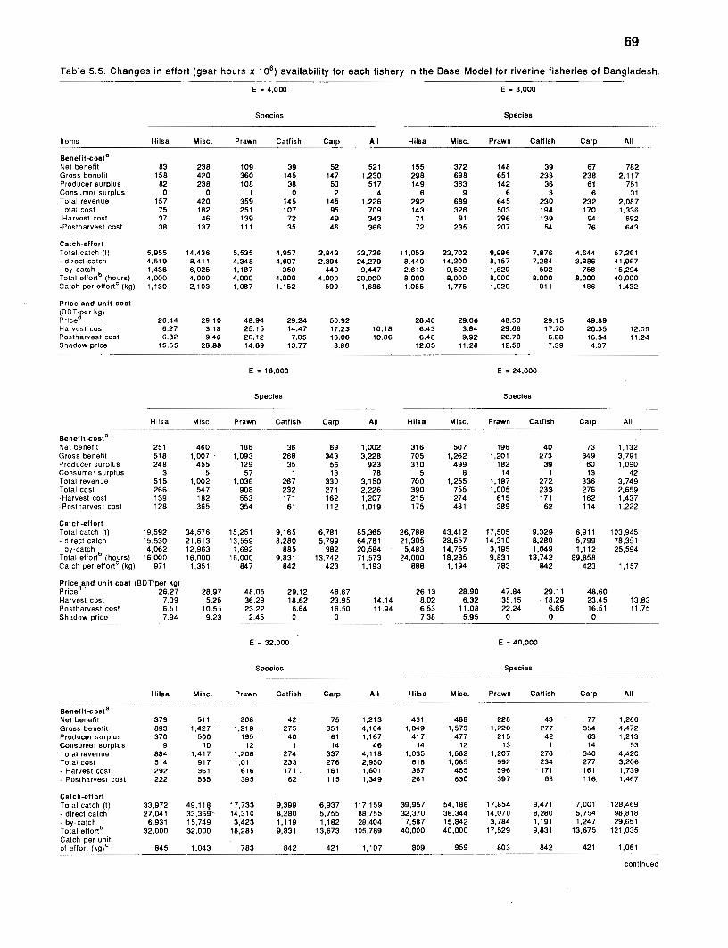
Table 5.5. Changes in effort (gear hours x lo6) availability for each fishery in the Base Model for riverine fisheries of Bangladesh.
Items
Species Species
Hilsa Misc. Prawn Catfish car^ All Hilsa Misc. Prawn Catfish Carp All
Benefit-costa Net benefit Gross benefit Producer surplus Consumer surplus Total revenue Total cost -Harvest cost -Pcstharvest cost
Catch-effort Totai catch (I) - direct catch - by-catch Total effortb (hours) Catch per effortC (kg)
Price and uni t cost ( B D T l p r kg) Price Harvest cost Postharvest cost Shadow price
Species Species
Hilsa Misc. Prawn Catfish Caro All Hilsa Misc. Prawn Catfish
~ e n e f i t - c o s t a Net benefit 25 1 460 Gross benefit 518 1.007 . Producer surplus 24 8 455 Consumer surplus 3 5 Total revenue 515 1.002 Total cost 266 547 -Harvest cost 139 182 -Postharvest cost 128 365
Catch-effort Total catch (I) 19,592 34.576 - d~rect catch 15.530 21 -61 3 - by-catch 4.062 12.963 Total effortb (hours) 16.000 16,000 Catch per effortC (kg) 971 1.351
P r ~ c e and uni t cost (BDTrper kg) priced 26.27 28.97 Harvest cost 7.09 5.25 Postharvest cost 6.51 10.55 Shadow ~ r l c e 7.94 9.23
Hilsa Misc.
Benefit-costa Net benefit Gross benefit Producer surplus Consumer surplus Total revenue Total cost - Harvest cost - Postharvest cost
car^ All
E = 32.000
Species
E = 40.000
Species
Prawn
208 1.21 9 195 12
1.206 1.011 61 6 395
Catfish Carp All
1,213 4.164 1.167
46 4.118 2,950 1,601 1,349
Hilsa Misc. Prawn Catfish Carp All
Catch-effort Total catch (I) 33.972 49,118 17.733 9.399 6.937 117.159 39.957 54.186 17,854 9,471 7.001 128.469 - d~rec t catch 27,041 33,369 14,310 8,280 5.755 88.755 32.370 38,344 14,070 8,280 5,754 98.818 - by-catch 6,931 15.749 3.423 1.119 1,182 28.404 7.587 15.842 3,784 1.191 1,247 29.651 Total effortb 32,000 32,000 18,285 9,831 13,673 105.789 40.000 40,000 17,529 9.831 13,675 121,035 Catch per unlt of effort lko\' 845 1.043 783 842 421 1.107 809 959 803 84 2 421 1,061
continued

Table 5.5 (continued)
Species Species
Hilsa Misc. Prawn Catfish Carp All Hilsa Misc. Prawn Catfish Carp All
Price and unit cost (BDTIkg) priced 26.01 28.85 47.82 29.1 1 48.59 25.91 28.82 47.81 29.10 48.55 Harvest cost 8.59 7.36 34.73 18.16 23.26 13.67 8.93 8.39 33.37 18.02 23.05 13.54 Postharvest cost 6.54 11.30 22.27 6.65 16.52 11.52 6.54 11.63 22.21 6.65 16.51 11.42 Shadow price 5.25 1.97 0 0 0
million Bangladgsh Taka (US$l = BDT32). gear hours x 10 .
'~a t i o of direct catch to total effort. d ~ s for prawn price indicates that of only small prawns; price of large prawns is fixed at BDT177lkg.
Table 5.6. Shadow prices of effort for various fisheries (Dual value in million BDT).
Available effort Shadow price in each fishery (gear hours x 10') (gear hours
x lo6 ) Hilsa Prawn Catfish Carp Misc.
Level of effort at which Dual value becomes zero 11 1,321
that a nonspecific effort allocation can bring higher net benefit to the society and a larger catch per unit of effort at all levels of effort availability. This is because, given that efforts are flexible, a nonspecific effort allocation would make interspecies allocation of effort in such a way that efforts will move from fisheries with lower shadow prices to fisheries with higher shadow prices. The process will continue until shadow prices in all fisheries become equal. For instance, as seen in Tables 5.5 and 5.6, when a total of 20,000 gear hours x 106 of effort are specified to be allocated equally among five existing fisheries, the shadow price of effort (expressed in gear hours x lo9) for the miscellaneous fishery is the highest (BDT28.88 million) while that for carp is the lowest (BDT8.86 million). On the other hand, as shown in Table 5.4, when the same effort is made unrestricted, the interspecies allocation will equate the shadow price of effort (gear hours x lo9) to BDT17.64 million for all fisheries, making the highest allocation to the miscellaneous fishery (7,274 gear hours x lo6) and the lowest allocation for carp (988 gear hours x 1 06).
Here again, it must be stressed that the increase of effort directed, e.g., against hilsa could actually lead to a rapid drop of catch and profits due to a failure of recruitment, an element not considered in the model.

Table 5.7. Behavior of the riverine fisheries of Bangladesh under alternative cost conditions (changes in the cost of harvesting from the Base Model).
Condition of cost
Items 50% 25% Base 25% 50% 100%
decrease decrease Model increase increase increase
Benefit-costa Net benefit Gross benefit Producer surplus Consumer surplus Total revenue Total cost -harvest cost -postharvest cost
Catch-effort Total catch ('000 kg) 305.65 230.06 173.16 130.23 96.58 54.13 -direct catch 245.87 184.26 139.86 104.67 77.36 44.30 -by-catch 59.77 45.80 33.31 25.56 19.22 9.83 Total effort (hourslb483,363 303,101 197,054 131,493 84,671 38,787 Catch per effort (kg/ gear hour x lo6)) 632 759 879 990 1,141 1,396
aln million Bangladesh Taka (US$1 = BDT32). gear hours x lo6.
Simulation of Cost and Demand Changes and Implications for Policy
In the supply-demand framework of the programming model, most of the policy and factor changes will affect the outcome through changes in the cost and price structure of the fisheries. Therefore, in the following sections efforts have been made to analyze the effects of changes in the cost and demand structure of the Base Model in terms of behavior ol the fisheries. Cost changes include shifts in the harvesting cost, while demand changes include changes in the aggregate price.
CHANGES IN THE COST OF HARVEST
The structure of cost functions for harvesting various species of fish from the rivers of Bangladesh was analyzed by performing systematic changes in the harvest cost functions used in the Base Model. Such changes were done in both directions (increase and decrease) from the level of Base Model harvest-cost functions.
Table 5.7 shows the aggregate results of variations of cost of harvesting in percentage terms of the Base Model costs. As seen in Table 5.7 a 25% decrease in the cost of harvest would allow aggregate efforts in the riverine fisheries of Bangladesh to expand by 54%, theoretically increasing the total landings by 33% and total net benefit by 63% from the levels shown by the resuits of the Base Model. However, the net benefit accrued would contribute more (in terms of percentage increase) to consumer surplus than to producer surplus. Thus, as a result of a 25% decrease in the cost condition of harvest, consumer surplus would increase by more than 500% (an increase from BDT94 million to BDT607 million) while producer surplus would increase by only 25% (an increase from BDT1,289 million to BDT1,653 million) from the Base Model levels.

Table 5.10. Changes in the availability of effort for a 25% decrease in the cost of harvest from the Base Model for riverine fisheries of Bangladesh.
Level of total effort (gear hours x 1 06)
20,000 40,000 80,000 120,000 200,000 303,101 Items - -
Benefit-costa Net benefit Gross benefit Producer surplus Consumer surplus Total revenue Total cost -Harvest cost -Postharvest cost
Catch-effort Total catch ('000 t) 37.35 -direct catch 27.52 -by-catch 9.84 Total effortb 20,000 Catch per unit of effort (kglgear hour x lo6) 1,867 Shadow price of effort (BDTlgear hour x lo3) 20.99
aln million Bangladesh Taka (US$l = BDT32). gear hours x lo6.
2 0 t ~ l l l l l l l l l l l ~ l l , O 0 40 80 120 150 200 240 ZBO
Effort (gear hours x 09)
t 0 . 6 A 1 1 1 1 1 1 1 1 1 1 1 1 1 1 J 40 80 120 160 Po 240 280
Effort (gear hours x lo9)
Fig. 5.9. Catch and effort under alternative cost conditions. Fig. 5.10. CPUE and effort under alternative cost conditions.
[ m Base Model
/#+=I 25% decrease
Effort ( gear hours x 10
Fig. 5.11. Gross benefit and effort under alternative cost conditions.
I Effort (gear hours x los)
Fig. 5.1 2. Cost and effort under alternative cost conditions.

As shown in Fig. 5.9 the movement of total landings at varying levels of effort availability under alternative cost conditions follows a steady pattern. A higher amount of total catch is predicted - again under the assumption of no stock-recruitment relationship - for higher levels of effort with catch increasing at a diminishing rate for all situations of cost. This implies a downward sloping curve of CPUE for all cost conditions, as shown in Fig. 5.10. Furthermore, as observed in Fig. 5.9, a higher total catch would be obtained at each given level of effort when the cost condition decreases and vice versa. This results in an increase in the CPUE when cost condition decreases and vice versa, particularly for relatively higher level of effort availability. Thus, as shown in Fig. 5.10, the CPUE curve would shift up for a decrease in the condition of cost and vice versa. This situation is equivalent to a stock change in a given fishing environment with resultant change in the CPUE, and a change in the cost of harvest. Therefore, the simulation of alternative cost conditions of harvest can as well be attribated to stock changes, with the resultant outcome being similar to cost changes.
A similar pattern is observed in the case of gross benefit and net benefit shown in Figs. 5.1 1 and 5.13, respectively. Thus, gross revenue as well as net revenue would be higher for lower cost conditions for all levels of effort availability and vice versa.
As for the cost of harvest (effort cost), shown in Fig. 5.12, however, the movement is still steady but the relationship is positive. A lower total cost of effort is incurred at lower levels of cost conditions and vice versa. This is because a change in the cost condition of harvest would also change the unit cost of effort proportionately.
A 25% decreose
25% increase
Base Model ,
I Effort (gear hours x lo9 )
Fig. 5.13. Net benefit and effort relationships under alternative cost conditions.
Also, when cost conditions change, the allocatim pattern of effort across fisheries changes. This is evident from Table 5.1 1. The inter-species reallocation of effort under alternative cost conditions would also produce differing effects on the pattern of landings of each individual species. For instance, for hilsa higher catches are recorded at higher cost conditions, whereas for prawn, lower catches are recorded at higher cost conditions, for a given level of aggregate effort (Table 5.11). The implication of such results is that if several interdependent fisheries are exploited by effort that is flexible to reallocation across fisheries, changes in the condition of cost of harvest may change

Table 5.1 1. Behavior of effort (gear hours x lo6) use and landings (t) of individual species at various levels of effort availability and under alternative cost conditions.
Available Cost Condition level of effort 25% increase 25% decrease Base Model
(gear - hour8 Direct By- Total Dlrecl By- Total Direct By- Total x 1 0 ) Effort catch catch catch Effort catch catch catch Effort catch catch catch
Hilsa 20,000 40,000 80.000
120.000 160.000 200,000 303.101
Prawn 20.000 40,000 80.000
120,000 160.000 200.000 303.101
Catfish 20,000 40,000 80,000
120,000 160,000 200,000 303,101
Carp 20,000 40.000 80.000
120.000 160,000 200.000 303.1 01
the effort allocation and landings pattern of individual fisheries, depending on the opportunity cost of effort relative to the CPUE in each fishery.
The shadow price of effort for alternative cost conditions are shown in Table 5.12 and plotted in Fig. 5.14. It is seen from Table 5.12 that the shadow prices of effort are lower for a cost increase and higher for a cost decrease at a given level of effort. In
A 25% decrease
1 25% increase / Base Model
Effort (gear hours x lo9
Fig. 5.14. Shadow prices of effort under alternative cost conditions.

Table 5.1 2. Shadow prices (BDT x 10' per gear hour x lo9) of effort under alternative conditions of cost of harvest.
Available Cost condition effort (gear hours 25% 25% Base x lo6) increase decrease Model
Level of effort at which Dual value becomes zero 131,493 303,101 197,054
terms of Fig. 5.14 this implies that an increase in the cost condition of harvest would shift the curve of shadow price down and vice versa. The implication of such movements of shadow prices across different cost conditions are that each additional unit of effort would result in a larger contribution to the net benefit when applied to a cost situation that is lower than the one assumed in the Base Model and vice versa.
CHANGES IN AGGREGATE DEMAND
Changes in the retail demand functions for various species of fish were simulated by changing the intercepts of the functions. Such changes imply changes in the aggregate demand attributable to changes in the population, real income, etc. The intercepts were shifted up and down by 10% and 20% from the Base Model demand intercepts.
Table 5.13 shows the aggregate outcome under alternative demand conditions. A decrease in the aggregate demand would reduce the level of effort while an increase in the aggregate demand would increase the level of effort as compared to the Base Model. The resultant effects on the landings (total catch), total cost and net benefit (producer and consumer surplus) would also be positive. As seen in Table 5.13 a 10% decrease in the aggregate demand for all fish species would decrease the level of effort by 28% from the Base Model level. This would reduce the total catch, total cost and net benefit by 20%, 26% and 32%, respectively. A 10% increase in the aggregate demand would increase the level of effort by 26% from the Base Model level. The model predicts that this would increase the total landings by 19%, total cost by 26% and total net benefits by 52%. Also since the level of effort changes with the changes in the aggregate demand, the CPUE would also change. Accordingly, the CPUE for the operating fishing units would be higher for a decrease in the aggregate demand and vice versa.
As for the individual fisheries, the effects of changes in the aggregate demand on total effort and total catch would also be positive (Table 52 - Appendix A). Effort use and landings would increase for all species if aggregate demand increases and vice versa. However, relative effects of a given change in aggregate demand would be different for each fishery. Table 5.14 shows the catch (direct catch and by-catch), price and effort for individual fisheries under alternative demand conditions. As for effort use, a decrease in aggregate demand from the Base Model level would decrease the effort use in carp, prawn and hilsa fisheries by as much as 36% 32% and 30%,

Table 5.13. Behavior of different riverine fisheries of Bangladesh under alternative demand conditions (changes in the demand intercept from the Base Model).
Items 20%
increase 10% Base
increase Model 10% 20%
decrease decrease
Benefit-costa Net benefit Gross benefit Producer surplus Consumer surplus Total revenue Total cost -Harvest cost -Postharvest cost
Catch-effort Total catch (t) 232,045 -direct catch 186,050 -by-catch 45,995 Total effortb (hours) 310,900 Catch per effortC
(kglgear hour x lo6) 746
"In million Bangladesh Taka (US$l = BDT32). gear hours x lo6.
'Ratio of total catch to total effort.
Table 5.14. Total catch, price and effort for individual species under alternative demand conditions.
Demand condition - - -
10% Base 10% decrease Model increase
Species Catch Price Effort Catch Price Effort Catch Price Effort (t) (BDTIkg) hour^)^ (t) (BDTlkg) (hours)" (1) (BDTIkg) hour^)^
Hilsa 59,816 (52,930)~
PrawnC 12,946 (9,560)
Catfish 9,017 (7,960)
Carp 5,602 (4,421
Misc. 51,690 (35.200)
Total 139,072 (1 10,071)
gear hours x lo6. b~ igures in parentheses indicate the direct catch. 'Price indicates that of small prawns only.
respectively, whereas there would be no change in the effort in the catfish fishery as compared to the effort levels for the respective fisheries in the Base Model. Again, a
increase in aggregate demand would increase the effort in the prawn fishery, for instance, by as high as 44% whereas there would be only 10% increase in the effort in the hilsa fishery.

With respect to catch as an outcome of effort use, particularly direct catch, the response of individual fisheries is different for changes in aggregate demand. Thus, as shown in Table 5.14, a 10% decrease in aggregate demand would result in a decline of direct catch of prawn, hilsa and carp by as much as 31°/0, 25% and 23% respectively, whereas that of catfish would remain unchanged at the Base Modei level. Similarly, a 10% increase in aggregate demand would increase the direct catch of prawn, miscellaneous fish and carp by as much as 34%, 32% and 28% respectively, whereas that of hilsa and catfish would only increase by 6% and lo%, respectively. The behavior of catch and effort to changes in aggregate demand, therefore, shows that prawn and carp fisheries are more sensitive to demand changes (in both directions), while the hilsa fishery is more sensitive for a decrease in aggregate demand.
Also, as expected, the equilibrium prices of all species would increase when demand increases and vice versa. Thus, as shown in Table 5.14, a 10% decrease in the aggregate demand would increase equilibrium price for hilsa by lo%, while a 10% decrease in the aggregate demand would reduce that of hilsa by 9.3%. The effects on prices of other groups is similar in magnitude, ranging between 8.6% and 10% for both increase and decrease in aggregate demand.
The behavior of the riverine fisheries for various given levels of effort under alternative demand conditions was also simulated through sensitivity analysis. The outcomes for each level of effort under alternative demand conditions show how the individual fisheries as well as their aggregate grow, responding to alternative market (demand) conditions. Effects of 10% changes from the Base Model are shown in Tables 5.15 and 5.16.
The movement of aggregate catch, CPUE and benefit (gross benefit) and cost of harvesting at varying levels of available effort and under alternative demand xmditions are shown in Figs. 5.15 to 5.18, respectively. At lower levels of effort, aggregate catch,
Table 5.15. Changes in the availability of effort for a 10% decrease in the aggregate demand from the Base Model for riverine fisheries of Bangladesh.
Level of total effort (gear hours x lo6)
Items 20,000 40,000 80,000 120,000 142,178
Benefit-cost Net benefita Gross benefit Producer surplus Consumer surplus Total revenue Total cost -Harvest cost -Postharvest cost
Catch-effort Total catch (t) 37,760 -direct catch 28,026 -by-catch 9,734 Total effortb (hours) 20,000 Catch per effortC
(kglgear hour x lo6) 1,888 Shadow price of effort
(BDTlgear hour x lo3) 14.8
aln million Bangladesh Taka (US$l = BDT32). gear hours x lo6 .
'Ratio of total catch to total effort.

" 200- 0 -
160- 4- - - 5 120- C - 0 0 80- - - 8 10% decrease 0
40- L -
Total ef fort (gear hours x 10 1 Total effort ( gear hours x l o 9 1
2.0-
Base Model 10% decrease
- 10% increase 4- 1.2- - W I.0-
2 0.81
Fig. 5.1 5. Catchand effort under alternative demand conditions.
0 0.61
0.4
0.2
Fig. 5.16. CPUE and effort under alternativedemand conditions.
- - - - -
8 10% decrease I0 % increase
O 0 4 j
O L b bo ' slo ' k o ' d o 2bo ' A 0 ' Total effort (gear hours x 10') I Total effort (gear hours x los )
"̂ 3.5- 2 11, 3.0- $ 2.5-
C 2.0 s - 5 - + l o - rn 8 0.5
Fig. 5.17. Gross benefit and effort under alternative demand conditions.
10% decrease
-
- 0 1 1 ' 1 1 ' 1 1 1 1 1 1 1 1
Fig. 5.18. Cost and effort under alternative demand conditions.
0 40 80 120 160 200 240
CPUE and cost of harvesting show little or no change under alternative demand conditions. Gross benefits are higher for higher levels of aggregate demand and vice versa. Consequently, net benefits shown in Fig. 5.19 would be higher at higher levels of aggregate demand. This is due mainly to the higher levels of equilibrium price showing higher willingness of consumers to pay.
The behavior of each fishery under two alternative demand conditions (10% decrease and increase) for varying levels of effort availability is shown in Tables 53 and 54 - Appendix A.
The shadow prices of effort under alternative demand conditions are shown in Fig. 5.20. At a given level of effort, the shadow prices of effort would be higher for higher levels of aggregate demand and vice versa, provided that effort is a binding variable. Also, in all cases of demand conditions the shadow prices would fall as the level of available effort increases. The implication of this result is that when demand condition improves through an increase in the aggregate demand each unit of effort would have a higher positive contribution to the net benefit. As a result, the limit to which effort could be expanded in order to achieve higher net benefit simultaneously would be higher. In other words, the shadow price of effort would become zero at a higher level of its use if aggregate demand increases. Thus, as seen earlier in Table 5.13, the

Table 5.16. Changes in the availability of effort for a 10% increase in the aggregate demand from the Base Model for riverine fisheries of Bangladesh.
Level of total effort (gear hours x lo6)
Items 20,000 40,000 80,000 120,000 160,000 200,000
Benefit-costa Net benefit Gross benefit Producer surplus Consumer surplus Total revenue Total cost -Harvest cost -Postharvest cost
Catch-effort Total catch (t) 37,760 -direct catch 28,026 -by-catch 9,734 Total effortb (hours) 20,000 Catch per effortC
(kglgear hour x 10') 1,888 Shadow price of effort
(BDTIgear hour x lo3) 22.58
'In million Bangladesh Taka (US$1 = BDT32). b ~ n gear hours x lo6. 'Ratio of total catch to total effort.
I I I I I I I 40 80 120 160 200 240 280
Total effort ( gear hours x 10' 1
Fig. 5.19. Net benefit and effort relationships under alternative demand conditions.
optimal level of effort is higher for increases in aggregate demand while lower for decreases in the aggregate demand.
Implications The above results of cost and demand changes can be interpreted in terms of
policy and factors that affect the bioeconomic and technological variables as well as those on the demand side of the market. Such factors include resource availability, CPUE, cost of fishing inputs, postharvest handling and processing costs, and market

10% decrease
40 80 120 160 200 240-
I Total effort (gear hours x 10')
Fig. 5.20. Shadow prices of effort under alternative demand conditions.
prices for fish and fish products. In terms of the model any policy would result in some parametric changes to the functional equations affecting directly or indirectly the CPUE, cost per unit of effort and output, and prices, (revenues and benefits). For instance, the impact of a stock reduction or stock enhancement can be viewed either in terms of a change in the catchability coefficient or a proportionate change in the CPUE. This in turn would imply a proportionate change in the cost per unit of catch. Similarly, a technological change that would increase the fishing power of the individual units of effort will imply some change (a short-term increase) in CPUE and hence, a decrease in the cost per unit of catch, if not cost per unit of effort. Further, a change in the price of constituent effort will affect the cost per unit of effort, and hence the cost per unit of catch. Similarly, changes in the aggregate demand and a change in consumer taste can be viewed in terms of a shift of the demand (intercept changes) and a change in the slope of the demand function, respectively. In effect, almost all changes in policy or management variables influence costs and or prices.

CHAPTER 6 POLICY IMPLICATIONS AND CONCLUSION
In Bangladesh riverine fisheries, the major concern is the presence of an oversized effort capacity (1 18%). Given that effort could be reduced to economically efficient levels (represented by the results of the Base Model) the existing riverine fisheries are capable of generating substantial net benefits (BDT1,383 million per annum) of which 96% accrues to producer surplus. Under the traditional management through leasing to private individuals such benefitlsurplus is either lost (at least partly) due to the overcapacity of the fishing fleet or captured (partly) as monopoly profits by the lease holders who act as middlemen between the resource owner (government) and the fishers. The government gets only a token amount of this benefit through open auctions of fishery rights.
Intervention into the system by a management entity capable of controlling the intensity of effort would help tap substantial positive net benefits from these fisheries. The surpluses could be used to support management costs and the program of effort reduction, including rehabilitation of displaced workerslfishers. The relative capacity of various fisheries and fishing grounds in generating this surplus can be made a basis for taxing purposes.
In the government's ongoing thrust to manage fisheries through a restrictive licensing system (under the New Fisheries Management Policy) uniformity of fees charged can be obtained by evaluating the relative benefit potentials of fisheries across river systems and environments. In other words, a differential intensity has to be applied with regard to taxation. Thus, fisheries and/ or fishing grounds which have more benefit potential would require more taxation than those of less potential. On. the basis of the results obtained from the Base Model, an estimate of the benefit potential of each individual fishery can be made in terms of producer surplus per unit of effort. Thus, the prawn fishery can be ranked as having the largest potential (BDT13,925/gear hour x 1 06), followed by miscellaneous fish (BDT10,753lgear hour x lo6), catfish (BDT5,141/gear hour x 1 06), carp (BDT4,834/gear hour x lo6) and hilsa (BDT4,015/gear hour x 106), respectively. Therefore, the highest rate of taxation should be on prawn fishing followed by miscellaneous fish, catfish, carp, and hilsa fishing.
Again, there are distributional implications of this surplus: provided that the surpluses are not fully taxed away this will raise the income level of the sectoral participants who will be allowed to remain in the fishery.
Finally, the present model sheds light on issues that require careful consideration in the government's management plans. Such issues include: ensuring a balance among regions and rivers in terms of effort allocation and benefit generation, and an equity in the distribution of benefits among primary producers (fishers), the trading and middlemen communities, and consumers.
While it is true that management can capture the fisheries benefits either partly or wholly through an appropriate rate of taxation on either inputs (effort), output or both to maintain an optimal level of effort, it is also necessary to improve landing, transport and communication infrastructures to correct the discriminatory cost and revenue structures between regions of fish harvest as well as between sectoral participants (e.g., fishers

and postharvest operators), and thereby ensure a balance in the distribution of benefits and/or profits among interest groups.
The previous chapters have developed a programming model of a fishery sector through which an assessment of the benefit potentials of fisheries exploitation and its end uses can be evaluated. Application of a programming technique is productive to analyze behavior of fisheries under alternative technoeconomic and market (price) conditions. However, despite the considerable extent in the programming framework of the model, its implementation has been limited to few interacting elements in the fishery process. This is due to the shortage of information on both biological and economic aspects of the riverine fisheries of Bangladesh. As such, on the basis of the short-run observations on the variables, the implications of the results for long-term behavioral stability of the fisheries require testing by future investigations. Particularly, model outputs referring to the yields and/or benefits that could be taken given an increase of present fishing effort must be taken with a grain of salt, because the model did not consider the impact of reduced (adult) broodstock on the production of (juvenile) recruits.
Such investigations would include scientific assessments of the level of stocks of important species and its dependence on the regime of the rivers, stock-recruitment relationships, study of the relationship between gear heterogeneity and fishing mortality across species and seasons, and the analysis of factors and channels of postharvest activities. If the information necessary for the analysis can be generated, the framework of the model can be expanded to include other bioeconomic systems (e.g., beels, floodlands, lakes and ponds).

ACKNOWLEDGEMENTS
This report is based on my Ph.D. thesis at Universiti Pertanian Malaysia (UPM). I would like to acknowledge the financial assistance of Ford Foundation and Winrock International toward the publication of this report.
I am thankful to the late Dr. Ian Smith and to Dr. Daniel Pauly, Dr. Roger Pullin, and Mr. Jay Maclean, and other ICLARM staff for their support and friendship while preparing this report.
Special thanks to Mr. Jay Maclean, Dr. D. Pauly and Ms. Letty Dizon for editing the manuscript and to Messrs. Ovidio Espiritu, Jr., Chris Bunao and Albert Contemprate for assisting with the drawings.
REFERENCES
Aguero, M. 1983. A bioeconomic conditional predictive trade model in fisheries: the hake fishery. University of Rhode Island, Kingston, Rhode Island. Ph.D. thesis.
LAguero, M. 1987. A bioeconomic model of Peruvian pelagic fishery, p.307-324. In D.Pauly and I. Tsukayama (eds.) The Peruvian anchoveta and its upwelling ecosystem: three decades of change. ICLARM Stud. Rev. 15, 351 p.
Aguero, M. and M. Ahmed. 1990. Economic rationalization of fisheries exploitation through management: experiences from the open-water inland fisheries management in Bangladesh, p. 747-750. In R. Hirano and I. Hanyu (eds.) The Second Asian Fisheries Forum. Asian Fisheries Society, Manila.
Agiiero, M., S. Huq, A.K.A. Rahman and M. Ahmed, Editors. 1989. Inland fisheries management in Bangladesh. Department of Fisheries, Dhaka, Bangladesh; Bangladesh Centre for Advanced Studies, Dhaka, Bangladesh; and International Center for Living Aquatic Resources Management, Manila, Philippines. 149 p.
Ahmed, N. 1983. Marketing of selected fishes in Bangladesh: a study in efficiency. Department of Marketing, University of Dhaka, Bangladesh. Ph.D. thesis.
Anderson, L.G. 1975. Analysis of commercial exploitation and maximum economic yield in biologically and technologically interdependent fisheries. J. Fish. Res. Board Can. 32(10): 1825-1 842.
Anderson, L.G. 1976. The relationship between firm and industry in common property fisheries. Land Econ. 52: 179-191.
Anderson, L.G. 1977. The economics of fisheries management. The Johns Hopkins Press, Baltimore, Maryland.
BCAS. 1987. Benchmark report: experimental project on improved management of open-water inland fisheries of Bangladesh. Bangladesh Center for Advanced Studies, Dhaka, Bangladesh.
BBS. 1984. Monthly statistical bulletin of Bangladesh. Bangladesh Bureau of Statistics, Dhaka, Bangladesh.
BBS. 1985. Statistical pocket book of Bangladesh, 1984-85. Bangladesh Bureau of Statistics, Dhaka, Bangladesh.
BBS. 1986. Statistical pocket book of Bangladesh 1986. Bangladesh Bureau of Statistics, Dhaka, Bangladesh.
BBS. 1989. Statistical yearbook of Bangladesh 1989. Bangladesh Bureau of Statistics, Dhaka, Bangladesh.
Beddington, J.R. and R.B. Rettig. 1983. Approaches to the regulation of fishing effort. FA0 Fish. Tech Pap. 243.
Beverton, R.J.H. and S.J. Holt. 1957. On the dynamics of exploited fish populations. Fish Invest. Min. Agric. Fish Food (G.B.) Ser. 11, 19. 533 p.
Bockstael, N. 1977. A market model for the New England groundfish industry. Agricultural Experiment Station Bull. No. 422, University of Rhode Island, Kingston, Rhode Island.
Booth, D.E. 1972. A model for optimal salmon management. U.S. Fish. Wildl. Sutv. Fish. Bull. 7O(2) : 497-506.
Bromley, D.W. and R.C. Bishop. 1977. From economic theory to fisheries policy: conceptual problems and management prescriptions, p. 281-302. In L.G. Anderson (ed.) Economic impacts of extended jurisdiction. Ann Arbor, Michigan.
Cauvin, D.M. 1979. Regulating access in Canada's inland fisheries. J. Fish. Res. Board Can. 36(7): 827-836.
Charles, A.T. 1988. Fishery socioeconomics: a survey. Land Econ. 64(3): 276-295.

Christy, F.T., Jr. 1973. Fishermen quotas: a tentative suggestion for domestic management. Occas. Pap. No. 19. Law of the Sea Institute, University of Rhode Island, Kingston, Rhode Island.
Christy, F.T., Jr. 1982. Territorial use rights in marine fisheries: definitions and conditions. FA0 Fish. Tech. Pap. No. 227. 9 p.
Clark, C. 1976. Mathematical bioeconomics: the optimal management of renewable resources. John Wiley, New York.
Clark, C.W. and G.R. Munro. 1975. The economics of fishing and modern capital theory: a simplified approach. J. Environ. Econ. Manage. 2: 92-106.
Clark, C.W. and G.R. Munro. 1980. Fisheries and the processing sector: some implications for management policy. Bell J. Econ. 1 l(2): 606-616.
Cook, B.A. and P. Copes. 1987. Optimal levels for Canada's Pacific halibut catch. Mar. Res. Econ. 4: 45-61.
Copes, P. 1970. The backward bending supply curve of the fishing industry. Scot. J. Polit. Econ. 17: 69-77.
Copes, P. 1972. Factor rents, sole ownership and optimum level of fisheries exploitation. Manchester School Economics and Social Studies 41 : 145-1 63.
Copes, P. 1986. A critical review of the ndividual quotas as a device in fisheries management. Land Econ. 62(3): 278-291.
Copes, P. and B.A. Cook. 1982. Rationalization of Canada's Pacific halibut fishery. Ocean Manage. 8: 151-175.
Crutchfield, J.A., Editor. 1965. The fisheries: problems in resource management. University of Washington Press, Seattle, Washington.
Crutchfield, J.A. 1979. Economic and social implications of the main policy alternatives for controlling fishing effort. J. Fish. Res. Board Can. 36(7): 742-752.
Crutchfield, J.A. and A. Zellner. 1962. Economic aspects of Pacific halibut fishery. US Dept. Interior (Washington) Fish. Industr. Res. l(1): 1-1 73.
Cunningham, S., M.R. Dunn and D. Whitmarsh. 1985. Fisheries economics: an introduction. Mansell Publishers Ltd., London.
DeVoretz, D. 1982. An econometric demand model for Canadian Salmon. Can. J. Agric. Econ. 30: 49-60.
DOFIBFRSS. 1982. Pilot surveys of rivers and beel fisheries. Department of Fisheries, Bangladesh Fisheries Resource Survey System, Dhaka, Bangladesh.
DOFIBFRSS. 1985. Fish catch statistics of Bangladesh, 1983-84. Department of Fisheries, Bangladesh Fisheries Resource Survey System, Dhaka, Bangladesh.
DOFIBFRSS. 1986. Fish catch statistics of Bangladesh, 1984-85. Department of Fisheries, Bangladesh Fisheries Resource Survey System, Dhaka, Bangladesh.
DOFIBFRSS. 1991. Fish catch statistics of Bangladesh, 1988-89. Department of Fisheries, Bangladesh Fisheries Resource Survey System, Dhaka, Bangladesh.
Duloy, J.H. and R.D. Norton. 1975. Prices and incomes in linear programming models. Am. J. Ag. Econ. 57: 591 -600.
Dunn, I.G. 1982. The hilsa fishery of Bangladesh, an investigation of its present status with an evaluation of current data. F1 .DP/BGDl81034. FAO, Rome.
FAOIRapport. 1986. Report on marketing of fish and shellfish in Bangladesh. Prepared by Rapport Bangladesh Ltd. for FAO. DP/BGD/79/015-3F1. 143 p.
Farrell, J.F. and H.C. Lampe. 1965. The New England fishing indust ry'/ functional markets for finned food fish II. Agricultural Experiment Station Bull. No. 380. University of Rhode Island, Kingston, Rhode Island.
Farrell, J.F. and H.C. Lampe. 1967. The revenue implications of changes in selected variables examined in the context of a model of the haddock market, p. 45-60. In F.W. Bell and J.E. Hazleton (eds.) Recent developments and research in fisheries economics. The New England Economics Research Foundation. Oceana Publishers Inc., Dobbs Ferry, New York.
Fox, W.W., Jr. 1970. An exponential surplus-yield model for optimizing.exploited fish populations. Trans. Am. Fish. Soc. 99: 80-88.

Squires, D. 1987. Fishing effort: its testing, specification, and internal structure in fisheries economics and management. J. Environ. Econ. Manage. 14: 268-282.
Storey, D.A. and C.E. Willis. 1978. Econometric analysis of Atlantic sea scallop markets. Department of Food and Resource Economics, University of Massachusetts, Amherst, Massachusetts.
Takayama, T. and G.G. Judge. 1971. Spatial and temporal price and allocation models. North- Holland Publishing, Amsterdam.
Tomek, W.G. and K.L. Robinson. 1981. Agricultural product prices. Cornell University Press, lthaca and London.
Tsai, C. and L. Ali. 1985 Open water fisheries (carp) management in Bangladesh. Fish. Info. Bull. 2(4):1-51.
Turvey, R. 1964. Optimization and sub-optimization in fishery regulation. Am. Econ. Rev. 54: 64- 76.
Ullah, M. 1985. Fishing rights, production relations, and profitability: a case study of Jamuna fishermen in Bangladesh, p. 211-223. In T. Panayotou (ed.) Small-scale fisheries in Asia: socioeconomic analysis and policy. International Development Research Centre, Canada.
Wang, D.H. 1976. An econometric study of Canadian sockeye salmon market. Oregon State University. 157 p. Ph.D. dissertation.
Wang, D.H., J.B. Dirlam and V.J. Norton. 1978. Demand analysis of Atlantic sea scallop fisheries. Department of Resource Economics, University of Rhode Island, Kingston, Rhode Island.
Wang, D.H. and J.J. Mueller. 1981. Intertemporal issues and economic analysis in fishery management under the Fishery Conservation and Management Act of 1976. In L.G. Anderson (ed.) Economic analysis for fisheries management plans. Ann Arbor, Michigan.
Wang, D.H., L.J. Goodreau and J.J. Mueller. 1986. Economics of Atlantic sea scallop management. Mar. Res. Econ. 3(2): 11 2-1 35.
Waugh, F.V. 1964. Demand and price analysis: some examples from agriculture. USDA Tech. Bull. 1316.
Waugh, F.V. and U.J. Norton. 1969. Some analysis of fish prices. Working Paper No. 32. Division of Economic Research, Bureau of Commercial Fisheries, Washington, DC.
Waugh, G. 1984. Fisheries management: theoretical developments and contemporary applications. Westview Press, Boulder, Colorado.
World Bank. 1991. Bangladesh Fisheries Sector review. World Bank Report. Weitzman, M. 1974. Free access vs private ownership as alternative systems for managing
common property. J. Econ. Theory 8: 225-239. Yahaya, J. 1988. Fisheries management and regulations in Peninsular Malaysia. Mar. Res. Econ.
5(2): 83-98. Zellner, A. 1961. Application of mathematical programming techniques to commercial fishery
conservation problems. FA0 Fish. Rep. 5: 515-534.

Appendix A Tables 33 to 54
T a b l e 3 3
Area o f Large Water Bodies i n Each Region o f Bangladesh by D i s t r i c t
( s q km)
R i v e r s and E s t u a r i e s Baor,
Region/ Jarnuna- Bee1 & Grand ~ i s t r i c t Meghna Padma B.Putra O t h e r s T o t a l Lakes T o t a l
N o r t h e a s t S y l h e t 0 Mymensingh 1 5 Comi l l a 276 T a n g a i l Dhaka 143 S o u t h e a s t Noakha l i 68 C h i t t a g o n g Ctg. H i l l s Nor thwes t Pabna Bogra Rangpur D i n a j p u r R a j s h a h i S o u t h w e s t F a r i d p u r 14 P a t u a k h a l i B a r i s a l 224 Khulna Jessore K u s h t i a T o t a l 740
Source : Water Area S t a t i s t i c s of Bangladesh, F i s h e r i e s I n f o r m a t i o n B u l l e t i n Vol. 2 (I), 1986. DOF.

Table 34
Number of Fishing Units and Fishing Boats Operating in Different Riverine Waters of Bangladesh
Meghna Padma J-B.putra Others Items (River 1) (River 2) (River 3) (River 4) Total
Fishinq unitsa Dry Season 10,117 2,228 1,989 17,006 31,340
( % I 3 2 7 6 54 100 Wet Season 15,722 2,922 1,728 19,283 39,655
4 0 7 4 4 9 100 Average 12,920 2,575 1,859 18,145 35,498
( % ) 3 6 7 5 51 100 Fishina 130atsb 24,641 9,049 3,065 N.A. 36,755
( % I 67 25 8 N.A. 100 -------------------------------------------------------- ........................................................ a: estimated based on monthly sample survey of operating
fishing units by BFRSS/DOF, Bangladesh for the period 1985-86 and 1986-87.
b: survey of fishing vilages and fishing boats by DOF.
Table 35
Distribution of Sample Fishing Units in the Selected Areas of Riverine Fishing in Bangladesh
......................................................
River No. of Sample as Group River District Samples % of boatsa ...................................................... Riv 1: Lower Neghna Comilla 50
Barisal 60 Upper Meghna Dhaka 15
Comilla 4 0 sub-total: 165
Riv 2: Lower Padma Faridpur 3 0 Dhaka 20
Upper Padma Rajshahi 25 sub-total: 75
Riv 3: Jamuna-B.putra Pabna 20 Rangpur 55
sub-total: 75 Riv 4: Garai-Madumati Faridpur 30
Old Brahinaputra Mymensingh 30 Tetulia Barisal 4 0 sub-total: 100
ALL Total : 415 ..................................................... ----------------------------------------------------- a: according to survey of fishing boats by DOF (unpub).


T a b l e 37
C o m p u t e d A v e r a g e C o s t of C a t c h ( A C ) E q u a t i o n s f o r R e p r e s e n t a t i v e ~ i s h i n g U n i t s i n
D i f f e r e n t R i v e r s of B a n g l a d e s h by Species and Season
A v e r a g e C o s t Species Season (AC) Mean S . D . M e a n S . D .
Prawn : - R i v e r 1 d r y A C = 6 4 . 7 4 + . 0 1 5 q
w e t A C = 7 3 . 8 0 + . 0 1 7 q - R i v e r 2 d r y A C = 7 0 . 3 3 + . 0 1 7 q
w e t A C = 8 0 . 9 9 + . 0 1 7 q - R i v e r 3 d r y A C = 1 0 . 3 8 + . 0 1 7 q
w e t A C = 2 4 . 1 7 + . 0 0 1 7 q - R i v e r 4 d r y A C = 3 0 . 3 6 + . 0 1 7 q
w e t A C = 2 6 . 3 6 + . 0 1 7 q C a t f i s h : - R i v e r 1 d r y A C = 1 4 . 2 9 + . 0 0 1 4 5 q
w e t A C = 2 6 . 5 5 + . 0 0 0 9 q - R i v e r 2 d r y A C = 3 0 . 3 6 + . 1 4 5 q
w e t A C = 2 8 . 3 6 - t . 0 0 0 9 q - R i v e r 3 d r y A C = 2 3 . 7 4 + . 0 0 1 4 5 q
w e t A C = 2 8 . 9 8 + . 0 0 0 9 q - R i v e r 4 d r y A C = 1 0 . 9 1 + . 0 0 1 4 5 q
w e t AC= 8 . 9 1 + . 0 0 0 9 q C a r p : - R i v e r 1 d r y A C = 1 7 . 6 6 + . 0 0 6 2 q
w e t A C = 2 8 . 0 0 + . 0 0 0 9 q - R i v e r 2 d r y A C = 2 2 . 4 3 + . 0 0 6 2 q
w e t A C = 1 8 , 4 3 + . 0 0 0 9 q - R i v e r 3 d r y AC= 5 . 8 8 + . 0 0 6 2 q
w e t A C = 1 1 . 4 4 + . 0 0 0 9 g - R i v e r 4 d r y A C = 2 8 . 2 0 + . 0 0 6 2 q
w e t A C = 1 6 . 2 0 + . 0 0 0 9 q M i s c l : - R i v e r 1 d r y A C = l 2 . 7 8 + . 0 0 3 1 5 q
w e t A C = l G . G 9 + . 0 0 1 7 q - R i v e r 2 d r y AC= 9 , 2 5 + . 0 0 3 1 5 q
w e t AC= 9 . 6 3 + . 0 0 1 7 q - R i v e r 3 d r y AC= 6 . 7 0 + . 0 0 3 1 5 q
w e t AC= 5 . 2 8 + . 0 0 1 7 q - R i v e r 4 d r y AC= 2 . 8 3 + . 0 0 3 1 5 q
w e t AC= 2 . 6 2 + . 0 0 1 7 q ------------------------------ ..............................
Source: B a s e d on e s t ima ted r e g r e s s i o n e q u a t i o n s for s a m p l e f i s h i n g u n i t s .
a : gear hou r s x l o 6 b: a m o u n t i n kg.

Table 3 8
Aggregate Average Cos t o f Catch (AC ) Equa t i ons f o r Var ious ~ i s h e r i e s i n t h e
R i v e r s of Bangladesh
S p e c i e s R ive r Season AC ~ q u a t i o n s
H i l s a R ive r 1
R i v e r 2
R ive r 3
Rive r 4
Prawn R ive r 1
Rive r 2
R ive r 3
Rive r 4
C a t f i s h R i v e r 1
Carp
Miscl.
R ive r 2
R ive r 3
R i v e r 4
R i v e r 1
R i v e r 2
R i v e r 3
R i v e r 4
R i v e r 1
Rive r 2
R ive r 3
R i v e r 4
d r y wet d r y w e t d r y w e t d r y w e t d r y w e t d r y w e t d r y w e t d r y w e t d r y w e t d r y w e t d r y w e t d r y wet d r y w e t d r y w e t d r y w e t d r y w e t d r y wet d r y w e t d r y w e t d r y w e t
Source: computed a t t h e average c a t c h per annum and based on sample AC e q u a t i o n s i n Tab l e 37-
Note: Q = t o t a l c a t c h ( '000 kg ) AC = ave rage cos t / kg .

T a b l e 39
Monthly Market Margin E q u a t i o n s f o r v a r i o u s S p e c i e s Landed from ~ i v e r s of Bangladesh
by Region and Season
S p e c i e s Region Season E q u a t i o n
H i l s a : Region A: Dry MM1.1.1= 5.73-0.01539Q1.1.1 Region A: W e t MM1.1.2= 3.48-0.00085Q1.1.2 Region B: A l l MT41.2 = 6.98-0.00003Q1.2 Region C: A l l MPI1.3 = 4.74-0.0076Q1.3
Smal l Prawn: Region A: Dry M134.1.1=16.00-0.0030Q4.1.1 Region A: W e t MM4.1.2=18.54+0.00125Q4.1.2 Region B: A l l MI44.2 =21.34+0.0033Q4.2 Region C: A l l MM4.3 =18.97+0.03244.3
Big Prawn: N a t i o n a l : A l l MM8.0 =22.00f0.03748.0
Carp : Region A : Dry MM2.1.1=20.44-0.0104Q2.1.1 Region A: W e t MM2.1.2=16.68-0.0133Q2.1.2 Region B: A l l MM2.2 =19.60-0.061Q2.2 Region C: A l l MM2.3 =14.26+0.0022Q2.3
C a t f i s h : Region A: A l l MM3.1 = 8.04-t-0.002Q3.1 Region B: Dry W13.2.1= 2.57f0.0063Q3.2.1 Region B: W e t MM3.2.2= 7.17-k0.0063Q3.2.2 Region C: A l l MM3.3 = 1.58-tO.0106Q3.3
M i s c e l l a n e o u s : Region A: A l l MM5.1 = 7.72f0.0017Q5.1 Region B: Dry MM5.2.1=11.75+00034Q5.2.1 Region B: W e t MM5.2.2= 9.63f0.00034Q5.2.2 Region C: A l l MM5.3 = 7.22+0.0030Q5.3
Source : Derived a s t h e d i f f e r e n c e between r e t a i l and e x - v e s s e l p r i c e s shown i n T a b l e s 11 and 12 ( C h a p t e r V ) .
Note: Q = q u a n t i t y i n thousand kg.


T a b l e 4 2
P e r c e n t a g e of BY-catch t o Direc t C a t c h f rom V a r i o u s F i s h e r i e s i n D i f f e r e n t R i v e r s o f
Bang ladesh i n Each S e a s o n
S p e c i e s of Direct C a t c h
S p e c i e s I4ilsa Prawn C a t f i s h Ca rp M i s c l . o f
By-ca tch Wet Dry Wet Dry Wet Dry Wet Dry Wet Dry
R i v e r 1 H i l s a Prawn C a t f i s h C a r p I l i s c l . R ive r 2 H i l s a Prawn C a t f i s h C a r p P l i s c l . R i v e r 3 H i l s a Prawn C a t f is11 C a r p M i s c l . R i v e r 4 H i l s a Prawn C a t f i s h C a r p Niscl. .......................................................... ----------------------------------------------------------
S o u r c e : F i e l d S u r v e y , 1987-88.

T a b l e 4 3
Percen tage D i s t r i b u t i o n of H a r v e s t of V a r i o u s Species from E a c h R i v e r t o D i f f e r e n t R e g i o n s of
B a n g l a d e s h i n E a c h F i s h i n g Season
W e t Season D r y Season
Species R e g . A R e g . B R e g . C T c t a l R e g . A R e g . B R e g . C T o t a l
H i l s a : - R i v e r 1 - R i v e r 2 - R i v e r 3 - R i v e r 4 P r a w n : - R i v e r 1 - R i v e r 2 - R i v e r 3 - R i v e r 4 C a t f i s h : - R i v e r 1 - R i v e r 2 - R i v e r 3 - R i v e r 4 C a r p : - R i v e r 1 - R i v e r 2 - R i v e r 3 - R i v e r 4 M i s c l . : - R i v e r 1 - R i v e r 2 - R i v e r 3 - R i v e r 4
S o u r c e : B a s e d on F i s h C a t c h S t a t i s t i c s by species, d i s t r i c t a n d r i v e r g r o u p ( 1 9 8 3 - 8 4 - 1 9 8 6 - 8 7 ) ,
DOF/BFRSS ( u n p u b l i s h e d ) .

T a b l e 4 7
Average S i z e of F i s h i n g Gear (Ne t ) P e r F i s h i n g U n i t f o r Var ious F i s h e r i e s i n
t h e R i v e r s o f Bangladesh ( s q m)
H i l s a : - w e t s e a s o n -d ry s e a s o n
Prawn: - w e t s e a s o n -d ry s e a s o n
~ a t f i s h : - w e t s e a s o n -dry s e a s o n
Carp: - w e t s e a s o n -d ry s e a s o n
M i s c l . : - w e t s e a s o n -d ry s e a s o n
Source : F i e l d s u r v e y ( 1 9 8 7 - 8 8 ) .

Table 4 8
Changes in Aggregate Effort (gear hours x lo6) Availability in the Base Model for Riverine Fisheries of Bangladesh
Items Hilsa Prawn Catfish Carp Miscl. All Hilsa Przwn Catfish Carp Miscl. All ................................................................................................ ~ e n e f it-costa Net Benefit 115.0 121.1 36.5 29.6 GrossBenefit 216.33640104.0 70.5 Producer Surplus (Pas) 102.9 119.8 36.3 29.1 Consumer Surplus (C.S.) 12.1 1.2 0.2 0.5 Total Revenue 204.1 362.8 103.9 70.0 Total Cost 101.3 243.0 67.6 40.9 -Harvest 51.3 131.3 43.1 12.0 -Post-harvest 50.0 111.7 24.4 28.9 Cztch-Effort Total catch (mt) 7,715 5,573 3,547 1,353 18,521 36,709 12,291 10,483 6,059 1,883 29,450 60,166 -directcatch 6,000 4,1203,200 91014,150 28,380 9,294 8,1605,5201,13421,596 45,704 -by-catch 1,715 1,453 647 443 4,371 8,329 2,997 2,323 539 749 7,854 14,462 Total effort 5,570 3,763 2,405 988 7,274 20,000 9,130 8,003 5,531 1,364 15,982 40,000 ~atchl~ffort~ (kg/gear hour x lo6) 1,0771,0951,331 921 1,945 1,835 1,018 1,020 998 838 1,351 1,504 Price,and Unit Cost ( ~ D ~ l k g ) p r i c e 26.46 48.94 29.28 51.77 29.1 26.38 48.45 29.21 51.47 29.01 Harvest Cost 6.65 23.55 12.15 8.86 4.75 8.87 6.53 26.62 15.7 9.42 6.16 10.86 Post-~arvest Cost 6.48 20.04 6.89 21.37 9.65 10.73 6.49 20.74 6.78 15.63 10.18 11.09

Table 4 9
~ e h a v i o u r o f D i f f e r e n t Fisheries i n the Rivers o f Bangladesh Under A l t e r n a t i v e Cost Cond i t ions
(Changes i n t h e Cost of ~ a r v e s t i n g from t h e Base Model)
I==="P=PPtl=====aP======P=I=========================================================================s==
BASE MODEL 253 inctease
Items Hilsa Prawn Catfish Carp Kiscl. A l l Wilsa Prawn Catfish Carp Miscl. ~ l l ____--_____------------------------------------------------------------------------------------------ ~enefit-costa Net Benefit 497.7 246.7 49.5 80.4 508.8 1,383.2 280.3 154.9 7.7 51 - 1 434.5 928.5 Gross benefit 2,025.4 l,21 9.5 271.2 359.1 1,758.8 5,634.1 1,509.0 747.5 248.3 277.2 ,370.6 4,152.5 Producer Surplus (P.S. 1 446.6 234.0 48.5 66.2 493.7 1,288-9 249.2 149.5 6.7 42.9 425.1 873.4 Consunar Surplus (C.S. ) 51.1 12.8 1.1 14.2 15.2 94.3 31.0 5.5 1.0 8.3 9.4 55.1 Total Revenue 1,974.3 1,206.8 270.2 344.9 1,743.6 5,539.8 1,478.0 742.1 247.3 268.9 1,361 - 2 4,097.4 Total Cost 1,527.8 972.8 221.7 278.7 1,250.0 4,250.9 1,228.7 592.6 240.6 226.0 936.1 3,224.0 -Harvest 1,017.5 574.7 159.6 161.2 522.1 2,435.2 851.2 350.3 182.9 136.8 407.5 1,928.7 -post-harvest 510.3 398.0 62.1 117.5 727.9 1,815.7 377.5 242.2 57.7 89.3 528.6 1,295.3 Catch-Effort Total Catch (mt 78,161 17,981 9,281 7,113 60,627 173,163 57,710 11,440 8,406 5,439 47,150 130,225 -direct catch 70,350 13,850 7,960 5,741 41,956 139,857 52,560 8,200 7,520 4,588 31,800 104,668 -by-catch 7,811 4,131 1,321 1,372 18,671 33,306 5,150 3,240 966 851 15,350 25,557 Total ~ f f o r t ~ 111.321 16,804 9,336 13,654 45,939 197,054 77,045 8.050 8,436 9,294 28,668 131,493 C a t c h / ~ f f o r t ~ ( k g / g e a r h o u r x l o 6 ) 632 824 853 421 91 3 879 682 1,079 891 494 1,109 990 price.and Unit Cost (BDT/X~] price0 25.26 47.79 29.11 48.49 28.76 25.61 48.37 29.14 49.44 28.87 Harvest Cost 13.02 31.96 17.20 22.67 8.61 14.06 14.75 30.62 21.55 25.15 8.64 8.87 Post-harvest cost 6.53 22.14 6.69 15.51 12.01 10.49 6.54 21.17 6.80 16.41 11.21 10.73 ---------5-------------------P------------------------------------------------------------------------ ___I_-_-- --------_---------- ......................................................................

Table 49 (continued ...)
I terns Hilsa Prawn Catfish Carp Miscl. All Hilsa Prawn Catfish Carp Miscl. All --_------------------------------------------------------------------------------------------------- ~enefit-costa Net Benefit 1 9 7 . 6 1 2 6 . 7 0.8 37.6 278.9 641.6 808.8 416.9 96.1 1 2 7 . 2 8 0 9 . 1 2 , 2 5 8 . 0 Gross ben. 7,040.7 470 .7 176 .5 184 .5 1 , 1 6 8 . 6 3 , 0 4 1 . 0 2 ,648.1 1,956.5 312.9 5 1 9.6 2 , 6 6 1 . 8 8 , 0 9 8 . 9 P.S. 1 8 4 . 4 1 2 4 . 8 0 . 4 34.1 2 7 2 . 6 616 .3 719.2 385.2 9 4 . 8 97.0 3 5 7 . 0 1 , 6 5 3 . 2 C.S. 13 .1 1.8 0.4 3.6 6.3 25.3 89.6 31.6 1.3 30.2 4 5 2 . 1 6 0 4 . 8 T. Rev. 1 , 0 2 7 . 5 4 6 8 . 8 1 7 6 . 1 180 .9 1 , 1 6 2 . 3 3 ,015 .7 2,558.5 1,924.8 3 1 1 . 6 489.4 2 ,209 .8 7 ,494 .1 T. Cost 843 .1 344.0 175 .7 146 .9 8 8 9 . 7 2 , 3 9 9 . 4 1 , 8 3 9 . 3 1 , 5 3 9 . 6 2 1 6 . 8 392 .4 1 , 8 5 2 . 7 5 ,840 .9 -Harvest 583.7 1 9 7 . 9 135 .2 88.9 4 5 0 . 8 1 , 4 5 6 . 5 1,174.1 854.8 1 4 5 . 2 2 2 2 . 5 521.8 2 ,918.5 -Post-harvest 2 5 9 . 5 146 .1 40.5 58 .0 4 3 8 . 9 943 .0 665.2 684 .8 71.6 169 .9 1 , 3 3 1 . 0 2 ,922 .5 Catch-Ef fort T. Catch(nt1 3 9 , 6 4 2 7 ,152 6,024 3,583 40 ,177 9 6 , 5 7 8 103 ,000 28,648 1 0 , 7 1 8 1 0 , 5 1 4 7 7 1 8 4 2 3 0 , 0 6 4 -direct catch 3 5 , 0 0 0 4 , 1 4 6 5 ,320 2 ,758 3 0 , 1 3 9 7 7 , 3 6 3 92,483 23 ,670 8 , 8 5 0 8 , 7 5 7 5 0 5 0 0 1 8 4 , 2 6 0 -by-catch 4 , 6 4 2 3 , 0 0 6 7 0 4 8 2 5 1 0 , 0 3 8 1 9 , 2 1 5 1 0 , 5 1 7 4,978 1 , 8 6 3 1 , 7 5 7 2 6 , 6 8 4 4 5 , 8 0 4 Tot21 l2ff0rtb 4 3 , 9 3 8 3 , 7 8 9 5,306 5 ,179 2 6 , 4 5 9 8 4 , 6 7 1 173 ,194 33 ,931 1 1 , 0 6 9 2 3 , 5 1 4 6 1 , 3 9 3 3 0 3 , 1 0 1 ~atch/~ffort' 7 9 7 1 , 0 9 4 1 , 0 0 3 5 3 3 1 , 1 3 9 1 , 1 4 1 534 698 8 0 0 3 7 2 a 2 3 7 5 9 Price-and Unit COS~(DDT/RCJ) priceu 25 .92 48.79 29 .23 50.50 28 .93 24.84 46.81 29.07 46 .55 2 8 . 6 3 Harvest Cost 14 .72 27.67 22.45 24.80 1 1 . 2 2 1 5 - 0 8 11 - 4 0 29.84 13.55 2 1 - 1 7 6 . 7 6 1 2 . 6 9 Post-har. Cost 6 .54 2 0 . 4 2 6.72 1 6 . 2 0 1 0 . 9 2 9.76 6.46 23.90 6.68 16 .16 17.24 1 2 . 7 0 ------------------------=----------------=---------------------------------------------------------- ........................ ---------------- ..........................................................

Table 4 9 ( c o n t i n u e d ...)
Items H i l s a Prawn C a t f i s h Carp M ~ S C ~ . All
~ e n e f i t - c o s t a Net Ben. 1,075.9 906.9 158.1 263.1 404.0 2,808.1 Gross ben, P.S. C . S . T. Rev. T . Cos t - H a w e s t -Pos t -harv C a t c h - E f f o r t T . Catch 132,070 45,837 12,433 15,711 98795 305,646 -dir. c a t c h 110,255 38,962 10,071 13,355 65229 245,872 -by-ca tch 14,615 6,875 2,362 2,356 33,566 59,774 T. J2ffor tb 275,011 66,037 13,609 41,734 86,972 483,363 C a t c h / E f f o r t C ( k g / g e a r h o u r x lo6) 430 530 740 320 750 632 p r i c e ,and Unit C o s t (BDrl?/Kg) priceU 24.33 45.18 29.02 43.58 28.46
a : m i l l i o n Bangladesh Taka (BDT) b: g e a r h o u r s x l o 6 . c: r a t i o o f d i r e c t c a t c h t o t o t a l e f f o r t . d: i n t h e c a s e o f prawn p r a c t i c e i n d i c a t e s t h a t o f o n l y s m a l l
prawns, p r i c e o f b i g prawn i s f i x e d a t BDT177/kg.

Table 5 0
Changes in the ~vailability of Effort (gear hours x lo6) for a 25% Increase in the Cost of Harvest from the Base Model for Riverine Fisheries of Bangladesh
Itens Hilsa Prawn Catfish Cerp Pliscl. All Ailsa Prawn Catfish Carp Miscl. All ................................................................................................ ~ e n e f it-costa Net Benefit 8 9 . 6 85 .2 25.8 34.9 2 6 0 . 4 495.8 1 8 2 . 9 1 2 3 . 1 20.1 42.2 306.9 6 7 5 . 3 Gross benefit 2 0 3 . 5 328 .6 Producer Surplus 89.3 84.3 Consumer Surplus 0 .3 0 .9 Total Revenue 2 0 3 . 2 3 2 7 . 7 Totzl Cost 1 1 3 . 9 243 .4 -Harvest 64.1 1 4 2 . 3
Catch-Effort Total Catch(nt1 7 . 6 9 1 5 . 0 2 3 -direct catch . 6 : 0 0 0 3: 5 6 1 -by-catch 1 , 6 9 1 1 , 4 6 2 Total Effort 5 . 5 7 0 3 . 2 6 1 catch/~ffort' 1 ; 0 7 7 1 ; 0 9 2 Shadow Price Price-and Unit Cost (BDT/K~) Price" 26 .42 48 .99 29.28 51.75 29.09

Table 50 ( c o n t i n u e d ...)
I terns Hi l sa Prawn Cat f i sh Carp Miscl. A l l H i l sa Prawn C a t f i s h Carp Miscl. A l l
~ e n e f i t - c o s t a N e t Ben. 273.8 146.6 22.9 56.7 370.1 869.9 294.1 158.4 9.7 51.1 413.3 926.5 Gross ben. 894.7 727.9 184.6 184.4 1,196.2 3,187.8 1,361.9 745.0 247.0 270.5 1,330.3 3,954.0 P.S. 263.7 141.4 22.3 53.1 363.4 843.9 271.5 153.0 8.7 43.3 407.6 884.0 C.S. 10.0 5.2 0.6 3.5 6.7 26.1 22.6 5.4 1.0 7.9 5.6 42.5 T. Rev. 884.7 722.7 184.0 180.9 1,189.5 3,161.8 1,339.3 739.6 246.0 262.6 1,324.7 3,912.1 T. Cost 621.0 581.3 151.8 127.8 826.1 2,317.9 1,067.8 586.6 237.3 219.3 917.03,028.1 -Harvest 398.2 318.8 118.9 69.7 374.2 1,309.8 726.5 348.8 180.0 132.3 407.5 3,020.1 -Post -harvest 222.0 232.6 42.9 58.0 451.9 1,008.1 341.3 237.9 57.4 87.0 509.5 1,233.0 Catch-Effort T. Catch 34,014 11,169 6,302 3582 41,130 96,197 52,112 11,397 8,442 5,303 45,868 123,122 - d i r . ca tch 29,228 8,160 5,520 2,673 30,059 75,640 46,978 8,160 7,520 4,251 31,800 98,709 -by-catch 4,786 3,009 782 909 11,071 20,557 5,134 3,237 922 1,052 14,068 24,413 T. E f f o r t 35,280 8,003 5,531 4,816 26,370 80,000 65.816 8,003 8,436 9,077 28,668 120,000 ~ a t c h / ~ f f orcc (kg/gear hour X lo6) 828 1,020 998 555 1,140 1,202 714 1,020 891 468 1,109 1,026 Shadow Price (BDT/gear hour x 103) 3.25 0.2 ?rice,and Unit Cost ( B D T / x ~ ) price" 26.01 48-40 29.20 50.50 28.92 25.70 48.37 29.14 49.52 28-88 Iiarvest Cost 11.71 31.23 18.87 19.47 9.10 13.62 13.94 30.60 21 -32 24.96 8.88 24.59 Post-har. Cost 6.53 6.53 6.53 6.53 6.53 6.53 6.53 6.53 6.53 6.53 6.53 6.53 ---------------------------------------------------------------------------------------------------- ....................................................................................................

Table 5 0 ( c o n t i n u e d . . . )
I t e m s Milsa Prawn c a t f i s h Carp ~ i s c l . A l l
~ e n e f i t - c o s t a --- N e t Ben . 2 8 0 . 3 1 5 4 . 9 7 . 7 5 1 . 1 4 3 4 . 4 9 2 8 . 5 Gross ben. 1 , 5 0 9 . 0 7 4 7 . 5 2 4 8 . 3 2 7 7 . 2 1 , 3 7 0 . 6 4 , 1 5 2 . 5 P.S. 2 4 9 . 2 1 4 9 . 5 6 . 7 4 2 . 9 4 2 5 . 1 8 7 3 . 4 C.S. 3 1 . 0 5 . 5 1 . 0 8 . 3 9 . 4 5 5 . 1 T. Rev. 1 , 4 7 8 . 0 7 4 2 . 1 2 4 7 . 3 2 6 8 . 9 1 , 3 6 1 . 2 4 , 0 9 7 . 4 T . Cost 3.,228.7 5 9 2 . 6 2 4 0 . 6 2 2 6 . 0 9 3 6 . 1 3 , 2 2 4 . 0 -Harves t 8 5 1 . 2 3 5 0 . 3 1 8 2 . 9 1 3 6 . 8 4 0 7 . 5 1 , 9 2 8 . 7 -Pos t -ha rv . 3 7 7 . 5 2 4 2 . 2 5 7 . 7 8 9 . 3 5 2 8 . 6 1 , 2 9 5 . 3 Catch-Ef f o r t T. Catch 5 7 , 7 1 0 1 1 , 4 4 0 8 , 4 8 6 5 , 4 3 9 4 7 , 1 5 0 1 3 0 , 2 2 5 - d i r . c a t c h 5 2 , 5 6 0 8 , 2 0 0 7 , 5 2 0 4 , 5 8 8 3 1 , 8 0 0 1 0 4 , 6 6 8 -by-catch 5 , 1 5 0 3 , 2 4 0 9 6 6 8 5 1 1 5 , 3 5 0 2 5 , 5 5 7 T. I2 f fo r tb 7 7 , 0 4 5 8 , 0 5 0 8 , 4 3 6 9 , 2 9 4 2 0 , 6 6 8 1 3 1 , 4 9 3 C a t c h l E f f o r t C ( k g / g e a r hour x lo6) 6 8 2 1 , 0 1 9 8 9 1 4 9 4 1 , 1 0 9 9 9 0 Shadow P r i c e (BDT/gear hour x lo3) 0 P r i c e a n d U n i t C o s t (BDT/ICg) ----a P r i c e 2 5 . 6 1 4 8 . 3 7 2 9 . 1 4 4 9 . 4 4 2 8 . 8 7 H a r v e s t Cos t 1 4 . 7 5 3 0 . 6 2 2 1 . 5 5 2 5 . 1 5 8 . 6 4 8 . 8 7 P o s t - h a r . C o s t 6 . 5 4 2 1 . 1 7 6 . 8 0 1 6 . 4 1 1 1 . 2 1 1 0 . 7 3
a : m i l l i o n Bangladesh Taka (BDT) . b : g e a r h o u r s x lo6. c : r a t i o o f d i r e c t c a t c h t o t o t a l e f f o r t . d : i n t h e c a s e o f prawn p r a c t i c e i n d i c a t e s t h a t o f o n l y s m a l l prawns, p r i c e o f b i g prawn i s fixed a t BDT177/kg.

Table 51 (continued . . . )
L = 200,000 E = 303,101
S p e c i e s Spscies
Items H i l s a P r a m C a t f i s h C a r p Miscl. A l l Ulsa Prawn C a t f i s h C a r p Miscl. A l l
~ e n e f it-costd N e t B e n e f i t 748.26 454.22 90.46 131.74 700.92 G r o s s b e n e f i t 1,824.16 P.S 707.26 C.S. 41 - 0 0 T o t a l Revenue 1,783.1 6 T o t a l C o s t 7,075.90 - H a r v e s t 618.13 - P o s t - h a r v e s t 457.77 Catch-Effort T o t a l C a t c h ( m t ) 70 ,203 - d i r e c t c a t c h 59,669 - b y - c a t c h 10,534 4,814 1,545 1,586 21,090 T o t a l E f f o r t
(Kg 6 8 1 717 806 476 81 8 920 534 698 800 372 823 759 Shadow P r i c e 2.72 0 P r i c e and Unit C O S ~ ( B D T / K ~ )
a : m i l l i o n BDT; b: g e a r hours x l o 6 ; c : r a t i o of d i r e c t c a t c h ( i n kg) t o t o t a l e f f o r t ; d : a s f o r prawn p r i c e i n d i c a t e s t h a t of o n l y s m a l l prawns; p r i c e of b i g prawn i s f i x e d atBDT177/kg.

Table 5 2
B e h a v i o u r o f D i f f e r e n t F i s h e r i e s i n t h e R i v e r s o f B a n g l a d e s h u n d e r A l t e r n a t i v e Demand C o n d i t i o n s
( C h a n g e s i n t h e demand i n t e r c e p t from t h e BASE MODEL)
B e n e f i t - C o s t a P
Net B e n e f i t 497.65 246.73 49.54 80.42 508.83 1,303.17 773.20 340.33 77.19 121 -47 787.05 2,099.24 G r o s s b e n e f i t 2,025.40 1,219.51 271 .24 359.11 1,758.81 5,634.07 2,452.00 1,713.91 334.97 494.40 2,941 .I3 7,936.41 P r o d u c e r S u r p l u s ( P . S . ) 446.60 233.98 48.47 66.22 493.65 1,288.92 711.78 318.42 75.64 99.82 290.41 1,496.08 Consumer S u r p l u s (C.S.) 51 -05 12.75 1 .07 14.20 15.18 94.25 61.42 21 .91 1.55 21 -65 496.64 603.16 T o t a l Revenue 1,974.35 1,206.76 270.17 344.91 1,743.63 5,539.82 2,390.58 1,692.00 333.42 472.75 2,444-49 7,333.25 T o t a l C o s t 1,527.75 972.78 221 -70 278.69 1,249.98 4,250.90 1,678.80 1,373.58 257.78 372.93 2,154.08 5,837.17 -Harvest 1,077.47 574.74 159.61 161.22 522.132,435.17 1,123.17 826.45 180.44 228.20 819.20 3,185.46 - P o s t - h a r v e s t 510-28 398.04 62.09 117.47 727.85 1,815.73 555.63 547.13 69.34 144.73 1,334.88 2,651 -71 Catch-Ef f o r t T o t a l c a t c h (at)78,161 17,981 9,281 7,113 60,627 173,163 86,023 23,720 10413 8,974 77,480 206,610 - d i r e c t c a t c h 70,350 13,850 7,960 5,741 41,956 139,857 74,900 18,560 8,730 7,333 55,324 164,847 - b y - c a t c h 7,011 4,131 1,321 1,372 18,671 33,306 11,123 5,160 1,683 1,641 22,156 41,753 T o t a l E f f o r t ' 1 1 1 ,321 16,804 9,336 13,654 45,939 197,054 122,932 24,205 10,837 17,723 72,298 247,995 Catch/EffortC (kq/gear hour x -lo6) 632 824 053 421 91 3 879 6 0 9 767 806 41 4 7 6 5 8 3 3 P r i c e , a n d U n i t cost ( B D T / X ~ ) ?riceL' 25.26 47.79 29.11 48.49 28.76 27.79 52.21 32.02 52.68 31.55 H a r v e s t C o s t 13.02 31.96 17.20 22.67 8.61 14.06 13.06 34-84 18.10 25.43 10.57 15.42 P o s t - h a r v e s t C o s t 6.53 22.14 6.69 16.51 12.01 10.49 6.46 23.07 6.66 16.13 17.23 12.83

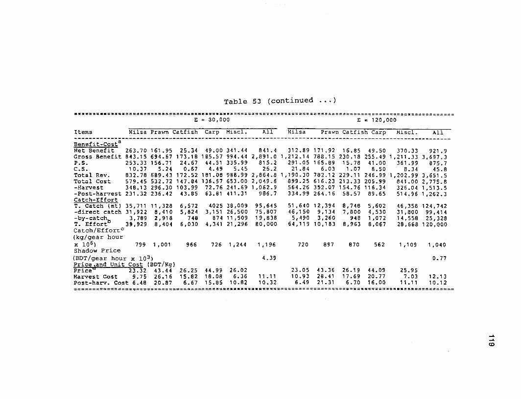


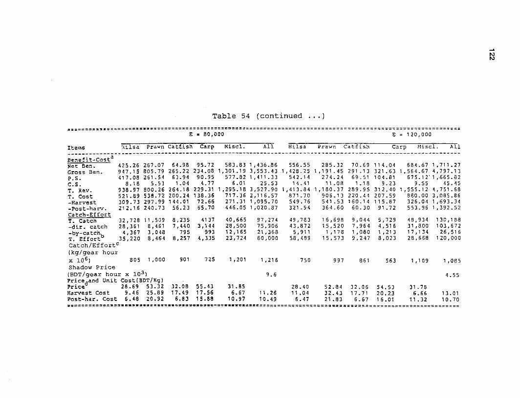


II1II .
=-
IIIIII
l1li
TITLES OF RELATED INTEREST ~
Theory and management of tropical fisheries. D. Pauly and G.L Murphy,Editors. 1982.ICLARMCont. Proc. 9, 360 p. US$17.50 surface; $28.50 airmail;"P200.
Phillppinetilapiaeconomlcs.LR. Smith, E.B.Torres and E.O.Tan, Editors. 1985.ICLARMCont. Proc. 12, 261 p. US$11 surface; $21 airmail;P1 00.
The economics of catfish farming Incentral Thailand. 1. Panayotou, S. Wattanutchariya,S.lsvilanondaand R.Tokrisna. 1982. Reprinted 1985.ICLARMTech.Rep. 4, 60p. US$6.50surface; $10 airmail;P80.
...
Production and marketing of milkfish InTaiwan: an economic analysis. C.S. Lee. 1983.ICLARMTech. Rep. 6, 41 p. US$6.30 surface; $9.50 airmail;"P80.
Small-scale fisheries of San Miguel Bay, Philippines: options for management andresearch. loR.Smith,D.PaulyandA.N.Mines.1983.ICLARMTech.Rep.11,80p.US$6.30surface; $9.50 airmail;"P80. .
Philippine municipal fisheries: a review of resources, technologyand socioeconomics.loR.Smith, M.Y. Puzon and C.N. Vidal-Libunao. 1980. Reprinted 1981, 1982. ICLARM Stud.Rev. 4, 87 p. US$5 surface; $12 airmail, P80.
l1li
I
The economics and management of Thai marine fisheries. T. Panayotou and S.Jetanavanich. 1987. ICLARM Stud. Rev. 4, 82 p. US$5 surface; $9 airmail; P90.
..
II .
HOW TO ORDER 'I)
Enquirers fromthe USAshould orderfrom ourexclusive distributor, the InternationalSpecialized Book Services, 5602 N.E. Hassalo Street, Portland, Oregon 97213-3640, to whom payment should be directed using the alrmailprice. Interested personsin Canada and Central and South America may also find ISBS a convenient source.
Enquirers in Europe may order from S. Toecha-Mlttler GmbH,Versandbuchhandlung, Hinde.rburgstrasse 33, D-61 00, FederalHepublic of Germany,
:.. using the airmail price.Enquirers elsewhere should address orders and payment (payable to ICLARM) in
US$ by international money order, bankdraft or Unesco cqupons to: The Editor,ICLARM, MC P.O. Box 1501, Makati, Metro Manila, Philippines. We can accept US$checks only if from from a US-based bank due to high clearan"ce fees of other banks.
Airmail is strongly recommended due to delays of up to six months and occasionallosses experienced with surface mail.
IIII'
III
a..
III
.