カルマンフィルタの基礎 - jmsfmml.or.jp · kalman filter basics t. enomoto 例: 酔歩...

カルマンフィルタの基礎

京都大学防災研究所榎本剛

[email protected]

2013年8月21日

第 17回データ同化夏の学校

Kalman Filter basics T. Enomoto

講義内容

本講義では，簡単な例を用いてカルマンフィルタの基礎について学ぶ。

• 線型フィルタ

• カルマンスムーザ

• 拡張カルマンフィルタ

• アンサンブル・カルマンフィルタ

第 17回データ同化夏の学校 1


副読本

• Rodgers, Clive, D, 2000: Inverse methods for atmospheric sounding:theory and practice. World Scientific, Singapore, 240pp.

• Kalnay, Eugenia, 2003: Atmospheric modeling, data assimilation andpredictability. Cambridge, UK, 341pp.

• 露木義・川畑拓矢（編）, 2008: 気象学におけるデータ同化. 気象研究ノート217, 日本気象学会, 東京, 277.



データ同化の原理

• 精度の良いデータに重く，悪いデータに軽く重みをつけて平均する。

xa =1/σ2

1

1/σ21 + 1/σ2

2

x1 +1/σ2

2

1/σ21 + 1/σ2

2

x2 (1)

1

σa2=

1

σ21

+1

σ22

(2)

• 予報を観測で修正する。（1: 予測xf, 誤差η，2: 観測y, 誤差ε）

xa = xf +1/σ2

ε

1/σ2η + 1/σ2

ε

(y − xf) (3)



カルマンフィルタ適用の前提

カルマンフィルタは，以下のような条件の下で有効である。

• 場の時間発展を記述するモデルがある。

xt = Mt(xt−1) + ηt (4)

• 連続的に観測データが得られている。

yt = Ht(xt) + εt (5)



線型フィルタ

基本的なカルマンフィルタは，線型問題に適用される。

xt = Mtxt−1 + ηt (6)

yt = Htxt−1 + εt (7)

予報

xft = Mtx

at−1 (8)

Pft = MtP

at−1M

Tt +Qt (9)



解析

Kt = PftH

Tt (HtP

ftH

Tt +R)−1 (10)

xat = xf

t +Kt(yt −Htxft) (11)

Pat = (I−KtHt)P

ft (12)

Ktは時刻 tにおけるカルマンゲインである。

この定式化では，時刻tまでの観測を連続的に同化し，時刻tにおける最適な推定値を与える。

カルマンゲインは最適内挿法の重みと同形であるが，予報誤差共分散が時間発展するとともに変化していく。



例: 酔歩

時間発展は次の式で与えられる。

xt = xt−1 + ηt (13)

ηtの分散は，σ2ηで与えられる。位置は，時刻t = 0, 1, ...において直接観測

され，欠測や不良データはないとする。

yt = xt + εt (14)

εtの分散は，σ2εとする。



予報

xft = xa

t−1 (15)

σft

2= σa

t−12 + σ2

η (16)

カルマンゲイン

Kt =σat−1

2 + σ2η

σat−1

2 + σ2η + σ2

ε

(17)

解析

xat = xf

t−1 +Kt(yt − xft) (18)

σat2 = (1−Kt)σ

ft

2(19)



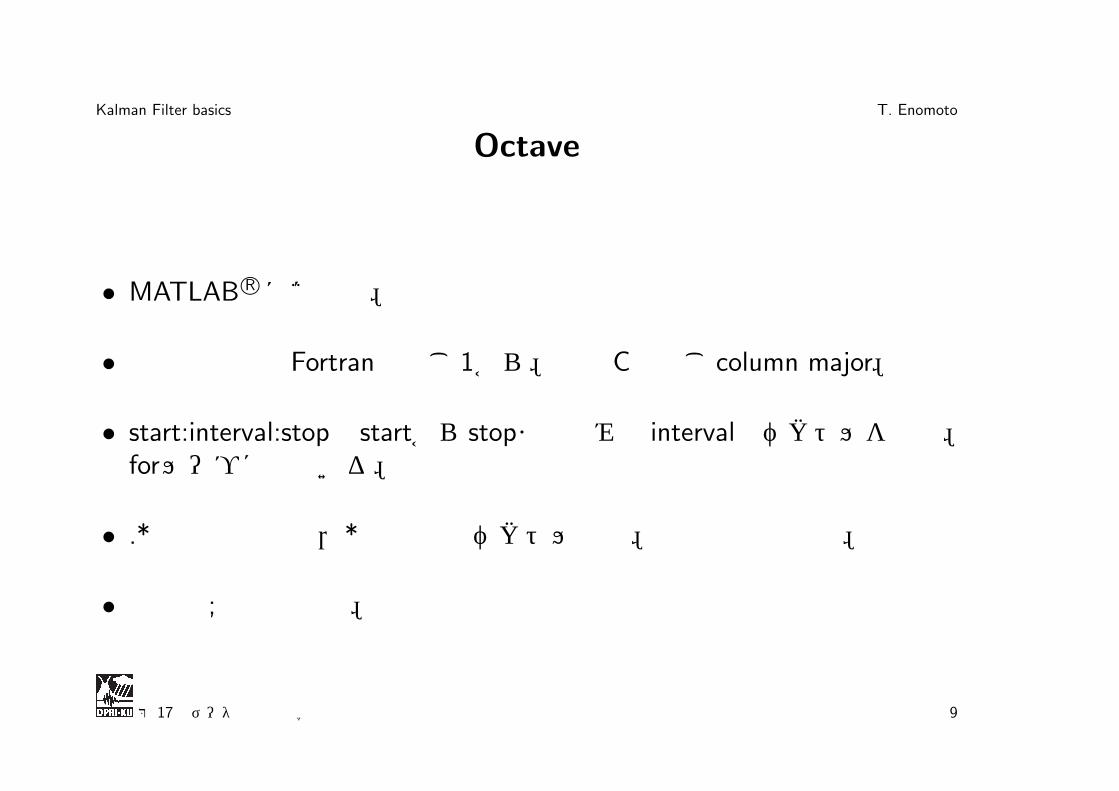
Octave

• MATLAB R⃝ほぼ互換。

• 配列の添字はFortranと同じ1から。でもCと同じcolumn major。

• start:interval:stopでstartからstopまで刻み幅intervalのベクトルを生成。forループにも用いる。

• .* は要素毎の積，* は行列やベクトルの積。累乗や商も同様。

• 行末の;は出力抑制。



酔歩: 数値実験

• ηの確率密度分布は，平均0，分散σ2η = 1の正規分布N(0, 1)に従う。

• σ2εの振幅は平均0，標準偏差2の正規分布に従い，観測毎に異なる。

N(0, σ2ε) = σεN(0, 1) =

√2N(0, 1)N(0, 1)



酔歩: 真値

ns t ep = 20 ;x t = zeros ( n s t ep+1, 1 ) ; % tru t hvq = 1 ; % model e r ror var ianceq = randn ( n s t ep+1, 1 ) ; % model e r rorf o r n=2: n s t ep+1

xt ( n ) = xt (n−1) + q (n ) ; % tru t hendfor



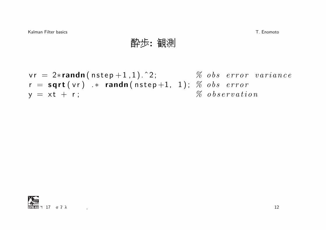
酔歩: 観測

v r = 2∗ randn ( n s t ep +1 ,1 ) .ˆ2 ; % obs error var iancer = sqr t ( v r ) .∗ randn ( n s t ep+1, 1 ) ; % obs errory = xt + r ; % obse r va t i on



-6

-5

-4

-3

-2

-1

0

1

0 5 10 15 20

distance

time



酔歩: カルマンフィルタ

x f (1 ) = xt ( 1 ) ;v f ( 1 ) = vq ;f o r n=2: n s t ep+1

x f ( n ) = xa (n−1); % fo r e c a s t NB. M=1v f ( n ) = va (n−1) + vq ;kg ( n ) = v f ( n ) / ( v f ( n ) + v r ( n ) ) ; % Kalman gainxa ( n ) = x f ( n ) + kg ( n )∗ ( y ( n ) − x f ( n ) ) ; % ana l y s i sva ( n ) = (1 − kg ( n ) ) ∗ v f ( n ) ;

endfor



-6

-5

-4

-3

-2

-1

0

1

0 5 10 15 20

distance

time



課題1

モデル誤差分散σ2ηだけでなく，観測誤差分散σ2

εも一定であるとき，解析誤差分散σa

t2は時刻t → ∞でどのようになるか述べよ。また，数値実験

でも確認せよ。



課題1 解答

σa2は一定になると考えられる。このとき，

σa2 = (1−Kt)(σa2 + σ2

η

)=

σ2ε

(σa2 + σ2

η

)σa2 + σ2

η + σ2ε

(20)

σa2 > 0となる解より次を得る。

σa2 =−σ2

η +√

σ4η + 4σ2

εσ2η

2(21)



0

0.5

1

1.5

2

0 5 10 15 20

variance

time



カルマンスムーザ

既に取得されている観測すべてを使ってデータ同化を行う場合は，解析時刻の前だけでなく後の観測も利用することができる。これをカルマンスムーザという。

• 前方にカルマンフィルタを適用し，予報値（アプリオリ）と解析値（推定値）を得る。

• 後方にカルマンフィルタを適用し，アプリオリと推定値を得る。

• 観測は一度だけ用いるという条件があるので，前方のアプリオリと後方の推定値，または前方の推定値と後方のアプリオリとの重み付き平均をとる。



後方推定を下線で表すと以下のようになる。

xft = Mtx

at+1 (22)

Pft = MtP

at+1M

Tt +Q

t(23)

Kt = PftH

Tt (HtP

ftH

Tt +R)−1 (24)

xat = xf

t +Kt(yt −Htxft) (25)

Pat = (I−KtHt)P

ft (26)

前方のアプリオリxftと後方の推定値xa

tを以下のように組み合せる。

P̃−1t =

(Pf

t

−1+Pa

t−1

)(27)

x̃t = P̃t(Pft

−1xft +Pa

t−1xa

t ) (28)



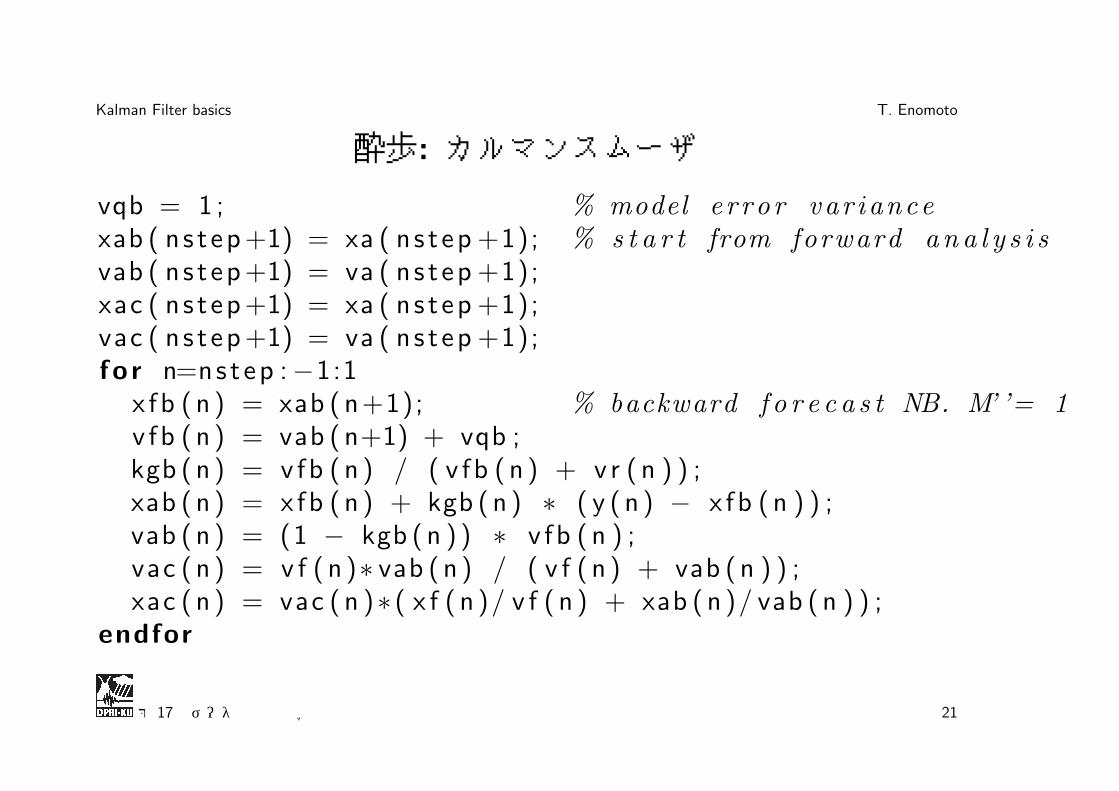
酔歩: カルマンスムーザ

vqb = 1 ; % model e r ror var iancexab ( n s t ep+1) = xa ( ns t ep +1); % s t a r t from forward ana l y s i svab ( n s t ep+1) = va ( ns t ep +1);xac ( n s t ep+1) = xa ( ns t ep +1);vac ( n s t ep+1) = va ( ns t ep +1);f o r n=ns t ep :−1:1

x fb ( n ) = xab ( n+1); % backward f o r e c a s t NB. M’ ’= 1v fb ( n ) = vab ( n+1) + vqb ;kgb ( n ) = v fb ( n ) / ( v fb ( n ) + v r ( n ) ) ;xab ( n ) = x fb ( n ) + kgb ( n ) ∗ ( y ( n ) − x fb ( n ) ) ;vab ( n ) = (1 − kgb ( n ) ) ∗ v fb ( n ) ;vac ( n ) = v f ( n )∗ vab ( n ) / ( v f ( n ) + vab ( n ) ) ;xac ( n ) = vac ( n )∗ ( x f ( n )/ v f ( n ) + xab ( n )/ vab ( n ) ) ;

endfor



-6

-5

-4

-3

-2

-1

0

1

0 5 10 15 20

distance

time



0

0.5

1

1.5

2

2.5

3

3.5

4

0 5 10 15 20

standard deviation

time



課題2

モデルMが時刻tに依存しないとき，前方及び後方過程は次のように書ける。

xt = Mxt−1 + ηt (29)

xt−1 = Mxt + ηt−1

(30)

ηtとxt−1，ηt−1とxtはそれぞれ無相関であるとき，xtとxt−1とのラグ

共分散を二つの方法で表記し，後方モデルMを前方モデルMで表せ。



課題2 解答

L ≡ E(xtxTt−1) = E(Mxt−1x

Tt−1 + ηtx

Tt−1) = MPf (31)

LT ≡ E(xt−1xTt ) = E(Mxtx

Tt + η

t−1xTt ) = MPf (32)

従ってM = PfMTPf−1

(33)



接線型モデル

基本解xに対する擾乱δxについて，時刻 t − 1から tまでの非線型モデルによる時間発展を考える。

xt = Mt(xt−1) (34)

xt−1の周りでTaylor展開を施すと

xt + δxt = Mt(xt−1 + δxt−1)

= Mt(xt−1) +Mtδxt−1 +O(|δx|2) (35)



ここで

Mt ≡∂M(xt)

∂x(36)

である。

従って，線型性が成り立つ場合，擾乱δxの時間発展は

δxt = Mtδxt−1 (37)

で記述される。

接線型モデルの随伴（adjoint）MTを随伴モデルという。



拡張カルマンフィルタ

モデルまたは観測演算子が非線型のときは，拡張カルマンフィルタが用いられる。予報値は，非線型モデルを用いて計算する。

xft = Mt(x

at−1) (38)

予報誤差共分散は，xat−1のまわりに線型化したモデルを用いて計算する。

Mt =∂M(xa

t−1)

∂x(39)

Pft = MtP

at−1M

Tt +Qt (40)



カルマンゲインは, 線型化された観測演算子を用いて計算する。

Ht =∂H(xf

t)

∂x(41)

Kt = PftH

Tt (HtP

ftH

Tt +R)−1 (42)

解析値の計算には，非線型の観測演算子を用いる。

xat = xf

t +Kt

[yt −H(xf

t)]

(43)

Pat = (I−KtHt)P

ft (44)



アンサンブル・カルマンフィルタ

• アンサンブル平均からのずれ δx = xfk − xfを誤差の標本とみなして，

予報誤差共分散を推定。

Pf ≈ 1

K − 1

∑k=1

Kδxfkδx

fk

T(45)

• 摂動観測法では，観測に摂動を与えて各メンバー独立に観測を同化。

• 平方根フィルタは，観測をアンサンブル平均に同化する。解析の摂動は予報の摂動の線型結合で表す。

δxat = δxf

tT (46)



アンサンブル・カルマンフィルタの利点

• 拡張カルマンフィルタよりも計算コストが低い。

• 接線型モデル，随伴モデルが不要。

• 時間発展する予報誤差共分散が陽に得られる。

• データ同化と同時にアンサンブル予報の初期擾乱を作成できる。



アンサンブル・カルマンフィルタの欠点

• モデルの自由度に比べてアンサンブル数が少ないため，サンプリング誤差が生じる。

• 偽りの相関による影響を取り除くため，局所化が必要。

• アンサンブル・スプレッドの過小評価を補うため，人工的なインフレーションが必要。

• 観測演算子やシステムには線型性，解析変数にはガウス分布を仮定している。



局所アンサンブル変換カルマンフィルタ

local ensemble transform Kalman filter (Hunt et al. 2007)

• 平方根フィルタの一つ。

• モデルの一部の領域で解析を行う。

• 領域毎に異なる線型結合をとることができるので，サンプリング誤差が軽減される。

• 並列計算機に適している。



LETKF: 解析

xa = xf +X fwa (47)

X fの第k列は予報の摂動δxf 重みは次のように求める。

wa = PaY fTR−1(y − yf) (48)

ここでY fは観測空間における予報摂動行列で，その第k列は

yfk − yf, yf

k = H(xfk) (49)

である。解析誤差共分散は

Pa = [(K − 1)I+ Y fTR−1Y f]−1 (50)

となる。



LETKF: アンサンブル更新

アンサンブルの更新は，解析誤差共分散行列を用いて

Xa = X fT (51)

T =√(K − 1)Pa (52)

のように行う。



アンサンブル・カルマンフィルタの予報解析サイクル



ALERA/ALERA2

AFES–LETKF experimental ensemble reanalysis

• 地球シミュレータ用大気大循環モデルAFESにLETKFを適用し，数値天気予報に用いられる全球大気観測データ（放射輝度を除く）を同化。

• ALERA (2005/5～2007/1): Miyoshi et al. 2007

• ALERA2 (2008/1～2010/8, 2010/8～2013/1): Enomoto et al. 2013

• 地球シミュレータセンターから入手可能（ALERA2は準備中）。



ALEDAS/ALEDAS2のデータフロー

AFES restartIC

t-3t-2t-1tt+1t+2t+3

merge

split

analysis

guess

LETKF

BC obs

Enomoto et al. 2013



海面気圧のスナップショット

ALERA CDAS

Miyoshi et al. 2007



ALERAスプレッド ALERA−CDAS

Miyoshi et al. 2007



観測システム実験: 氷上ブイによる気圧観測

Southern Hemisphere high latitudes. ALERA is open forscientific use and is distributed at http://www.jamstec.go.jp/esc/afes/alera/.[6] In this study, we regarded the 6-hourly ALERA data

as the control run (CTL). When producing ALERA data,patches of uniform grid spacing were used in LETKF forerror covariance localization. Contraction of the patches inthe zonal direction near the poles caused some discontinu-ities, particularly in the ensemble spread, due to excessivelocalization. AlthoughMiyoshi et al. [2007b] have proposeda new version of LETKF that does not require local patches,we used the version with local patches to allow forcomparisons with the original ALERA product. As will beshown below, discontinuities did not significantly affect ourevaluation of the impact of buoys in the Arctic region. In thetest run (ARC), the same observational data set, exceptwithout surface pressure observations north of 70 !N, wereassimilated using the identical system that producedALERA. These products include the analysis ensemblemean and analysis ensemble spreads of wind, temperature,humidity, dew point depression, and geopotential height at17 pressure levels between 10 and 1000 hPa. For this study,we examined the period from June 2006 to January 2007,during which many drifting buoys were deployed justbefore the International Polar Year (IPY). Further, the sea-ice extent in summer 2006 was relatively larger than that inthe summers of 2005, 2007, and 2008. Therefore, thisperiod is suitable for evaluating the impact of Arctic buoys.

3. Effect of Arctic Drifting Buoys

[7] Figure 1a shows the ensemble spread of sea levelpressure (SLPsprd) for CTL in August 2006. Because of thedense network of surface meteorological stations over land,the SLPsprd was extremely small in those areas (less than 1hPa). In contrast, SLPsprd over the Arctic Ocean wasgenerally much larger (more than 2 hPa) than that over

land. However, over the Beaufort Sea, where there wererelatively numerous drifting buoys on multi-year ice, theSLPsprd was relatively small. These characteristics were alsofound in other variables (e.g., air temperature and windspeed) and other months. The ARC results show largeSLPsprd over the Beaufort Sea (Figure 1b). The largerSLPsprd in the eastern Arctic suggests that buoy dataimproved the analysis accuracy both locally and over theentire Arctic region.[8] Figure 2a shows a time series of the difference (ARC!

CTL) in the ensemble spread of SLP (DSLPsprd) averagedover a dense-buoy area (the area is shown in Figure 1). TheDSLPsprd was always positive (1–3 hPa) during the anal-ysis period, suggesting that buoy data are effective inmaintaining SLP accuracy in all seasons, even thoughthe buoys drift. The stepwise increase in DSLPsprd at thebeginning of August would have been caused by thedeployment of six additional buoys in this region duringthe month (shading in Figure 2a). This result confirms thatdensely located drifting buoys contribute to more accuracyin SLP. As a whole, the difference (ARC ! CTL) in the SLPensemble mean (DSLPmean) had a negative bias (bars inFigure 2b) with larger amplitude in fall and winter than insummer partly due to the enhanced Beaufort high andfrequent passage of cyclones in fall and winter. However,there was no clear correlation between DSLPmean (Figure2b) and DSLPsprd (Figure 2a) although the correlationbetween DSLPmean and SLPmean itself (black line in Figure2b) was high. This result suggests that without the buoydata, the spatial patterns of high and low pressure systemsover the Beaufort Sea tend to be smoothed. The smootherSLP field (and higher pressure levels) would dampen thepressure gradients and winds.[9] The negative bias of DSLPmean should result in

modulated air temperature near the surface. Figure 2c showsa time series of the ensemble mean difference of air

Figure 1. Analysis ensemble spread of SLP in August 2006 for (a) CTL (b) and ARC. Dots depict the positions of theArctic drifting buoys. The thick line denotes ice concentration grater than 15%. The area enclosed by the dashed line is usedin Figure 2.

L08501 INOUE ET AL.: IMPACT OF ARCTIC DRIFTING BUOYS L08501

2 of 5

Inoue et al. 2009



観測システム実験: インド洋でのゾンデ観測Propagation of Observation Impact through Tropical 651

(a)

(b)

(c)

Figure 8. Horizontal distribution of the vertically integrated analysis ensemble spread (coloured every 10 m between 50 and 130 m and contoured every50 m) in (a) EX1 and (b) EX2 and (c) the vertically averaged analysis spread reduction rate (coloured) and the appearance frequency of the significantspread difference (contoured every 2% between 2% and 10%) in the layer of 1000–100 hPa averaged from 22 October to 2 December against geopotentialheight. Black dashed rectangles in (c) represent the area used to compute averages in Figure 9.

the Equator, z = 5000 m is a representative geopotentialheight, and Hs = 7300 m is a scale height in the tropicaltroposphere. The actual latitudinal positions are shiftednorthward by !10" because the 20 # 20 degree box can betaken as the average position. This latitudinal dependencyof the analysis spread reduction rate also corroborates thefinding that the dominant phenomenon in propagation ofobservation information to the east is the Kelvin waves.

Another factor that should contribute to the analysisspread reduction rate is the effect of the duration of theadditional observations. The time-averaged analysis spreadreduction rates for Cimaron, Chebi, and Durian, which are0.31%, 057%, and 3.18%, respectively, could include effectsof the duration of additional observations. Table II showsthe time-averaged analysis spread reduction rate from EX2to EX5 for each typhoon. The rates for Cimaron, Chebi, andDurian are interpreted as follows:

Cimaron: The assimilation of the MISMO data from3 days before genesis in EX2 for 17 days (22 October–7 November) results in a 0.17% higher spread reduction rate

than assimilation from 6 days after genesis in EX3 for 5 days(1 November–5 November).

Chebi: The assimilation of MISMO data from 16 daysbefore genesis in EX2 for 25 days (22 October–15 November)

• results in a 0.53% higher spread reduction rate thanassimilation from 7 days before genesis in EX3 for5 days (1–5 November), and

• results in a 0.31% higher spread reduction rate thanassimilation from 2 days before genesis in EX 4 for10 days (6–5 November).

Durian: The assimilation of the MISMO data from 33 daysbefore genesis in EX2 for 42 days (22 October–2 December)

• results in a 3.09% higher spread reduction rate thanassimilation from 24 days before genesis in EX3 for5 days (1–5 November),


Copyright c$ 2011 Royal Meteorological Society Q. J. R. Meteorol. Soc. 137: 641–655 (2011)

Propagation of Observation Impact through Tropical 651

(a)

(b)

(c)

Figure 8. Horizontal distribution of the vertically integrated analysis ensemble spread (coloured every 10 m between 50 and 130 m and contoured every50 m) in (a) EX1 and (b) EX2 and (c) the vertically averaged analysis spread reduction rate (coloured) and the appearance frequency of the significantspread difference (contoured every 2% between 2% and 10%) in the layer of 1000–100 hPa averaged from 22 October to 2 December against geopotentialheight. Black dashed rectangles in (c) represent the area used to compute averages in Figure 9.

the Equator, z = 5000 m is a representative geopotentialheight, and Hs = 7300 m is a scale height in the tropicaltroposphere. The actual latitudinal positions are shiftednorthward by !10" because the 20 # 20 degree box can betaken as the average position. This latitudinal dependencyof the analysis spread reduction rate also corroborates thefinding that the dominant phenomenon in propagation ofobservation information to the east is the Kelvin waves.

Another factor that should contribute to the analysisspread reduction rate is the effect of the duration of theadditional observations. The time-averaged analysis spreadreduction rates for Cimaron, Chebi, and Durian, which are0.31%, 057%, and 3.18%, respectively, could include effectsof the duration of additional observations. Table II showsthe time-averaged analysis spread reduction rate from EX2to EX5 for each typhoon. The rates for Cimaron, Chebi, andDurian are interpreted as follows:

Cimaron: The assimilation of the MISMO data from3 days before genesis in EX2 for 17 days (22 October–7 November) results in a 0.17% higher spread reduction rate

than assimilation from 6 days after genesis in EX3 for 5 days(1 November–5 November).

Chebi: The assimilation of MISMO data from 16 daysbefore genesis in EX2 for 25 days (22 October–15 November)


• results in a 0.31% higher spread reduction rate thanassimilation from 2 days before genesis in EX 4 for10 days (6–5 November).

Durian: The assimilation of the MISMO data from 33 daysbefore genesis in EX2 for 42 days (22 October–2 December)

• results in a 3.09% higher spread reduction rate thanassimilation from 24 days before genesis in EX3 for5 days (1–5 November),


Copyright c$ 2011 Royal Meteorological Society Q. J. R. Meteorol. Soc. 137: 641–655 (2011)

Moteki et al. 2011



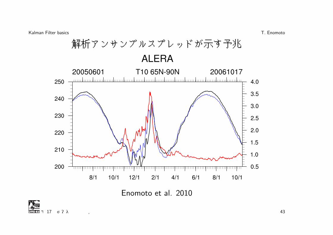
解析アンサンブルスプレッドが示す予兆

Enomoto et al. 2010



ランダム誤差を考慮した弱拘束随伴法

ランダム誤差を考慮する場合は，次の予報方程式を用いる。

xt = Mt−1(xt−1) + ηt−1 (53)

評価函数は次のようになり，初期値x0及びランダム誤差ηtを推定する。

J =1

2(x0 − xb

0)TB−1(x0 − xb

0)

+1

2

T∑t=0

(Htxt − yt)TR−1

t (Htxt − yt)

+1

2

T−1∑t=0

ηTt Q

−1t ηt (54)



ラグランジュ函数

L = J +

T∑t=1

[Mt−1(xt−1) + ηt−1 − xt]Tλt (55)

評価函数の勾配は

∇x0J =∂J

∂x0+

T∑t=1

MT0M

T1 · · ·MT

t−1

∂J

∂xt(56)

と表されることから，λtは以下を満たす。

λt+1 = 0 (57)

λt = MTt λt+1 +

∂J

∂xt(t = T, T − 1, ..., 0) (58)



ここで

∂J

∂x0= HT

0R−10 [H0(x0)− y0] +B−1(x0 − xb

0) (59)

∂J

∂xt= HT

t R−1t [Ht(xt)− yt] (60)

このときδL = δJとなり次を得る。

∇x0J = λ0 (61)

∇ηtJ = Q−1t ηt + λi+1 (t = 0, 1, ..., T − 1) (62)



例: 酔歩

評価函数

J =(x0 − xb)

2

2σ2b

+

T∑t=0

(xt − yt)2

2σ2rt

+

T−1∑t=0

η2t2σ2

η

(63)

勾配

∇x0J =x0 − xb

σ2b

+

T∑t=0

xt − ytσ2rt

(64)

∇ηtJ =ηtσ2η

+

T∑t=t+1

xt − ytσ2rt

(65)



酔歩: 随伴法

• 初期値x0とモデルのランダム誤差qを推定。

• x (t ̸= 0)はモデルで予測。

• コスト函数，勾配を計算。

• 線型探索をして降下法，共役勾配法の刻み幅を決定。

• ソースは長いので省略。

• 収束が遅い。ランダムだから?



-6

-5

-4

-3

-2

-1

0

1

0 5 10 15 20

distance

time



まとめ

• カルマンフィルタ: 解析時刻まで得られた連続的な観測を逐次的に同化。重みは最適内挿法と同形，誤差の少ないデータに大きな重み。

• カルマンスムーザ: 解析時刻より先のデータも利用できる場合，カルマンフィルタを後方にも適用，前方の予報と組み合わせ誤差をより減少。

• 拡張カルマンフィルタ: モデルと観測演算子を線型化することで非線型問題にも適用可。

• アンサンブル・カルマンフィルタ: アンサンブル予報を使って予報誤差共分散を近似。


カルマンフィルタの基礎 - jmsfmml.or.jp · kalman filter basics t. enomoto 例: 酔歩...

Documents