FALL 2006 EXAM M SOLUTIONS

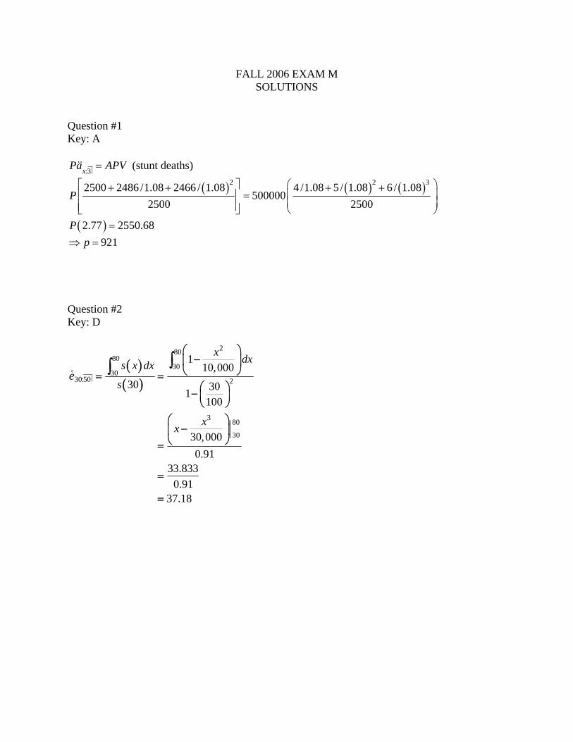
Question #1 Key: A

:3xPa APV=&& (stunt deaths)

( )22500 2486 /1.08 2466 / 1.082500

P⎡ ⎤+ +⎢ ⎥⎢ ⎥⎣ ⎦

( ) ( )2 34 /1.08 5/ 1.08 6 / 1.08500000

2500

⎛ ⎞+ +⎜ ⎟=⎜ ⎟⎝ ⎠

( )2.77 2550.68P = 921p⇒ =

Question #2 Key: D

( )( )

28080

3030

30:50 2

3 80

30

110,000

30 301100

30,0000.91

33.8330.91

37.18

x dxs x dx

s

xx

eo⎛ ⎞−⎜ ⎟

⎝ ⎠= =⎛ ⎞− ⎜ ⎟⎝ ⎠

⎛ ⎞−⎜ ⎟

⎝ ⎠=

=

=

∫∫

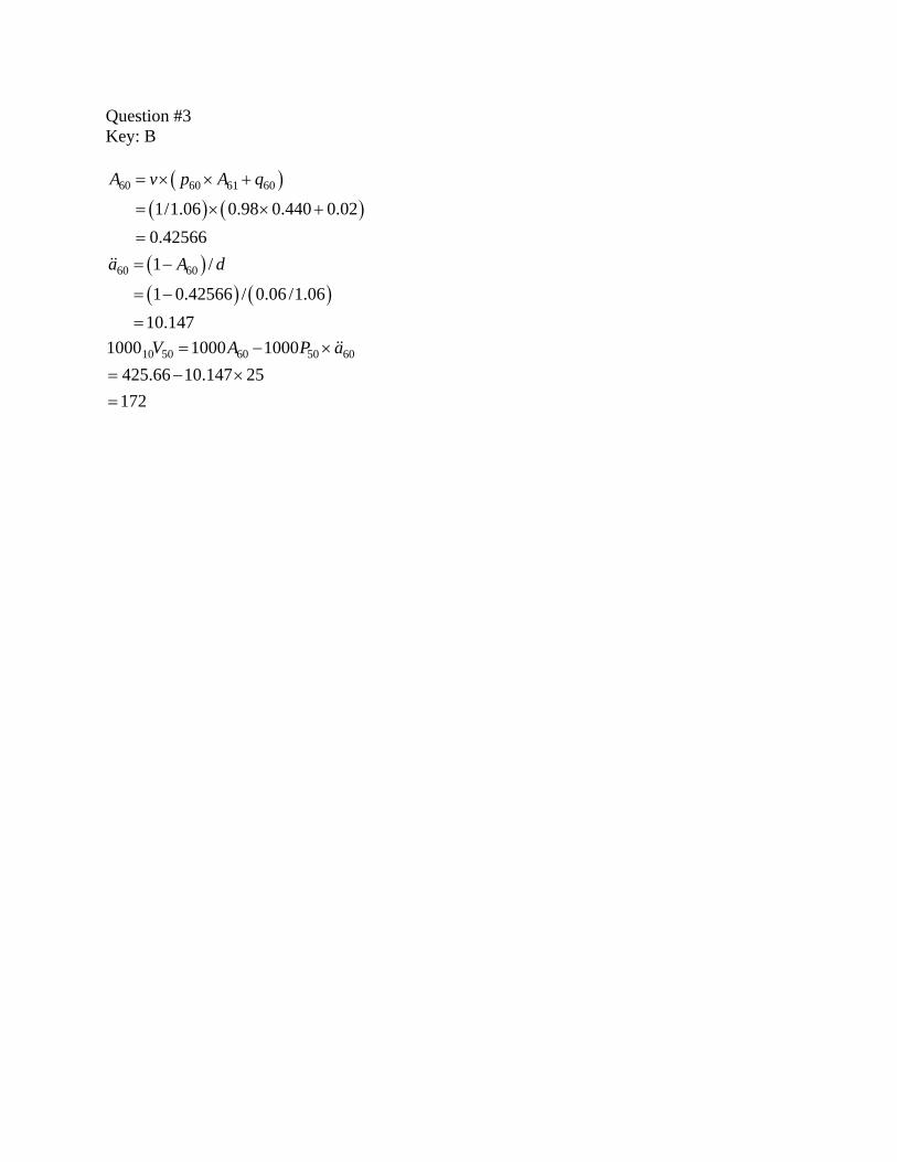
Question #3 Key: B

( )( ) ( )

60 60 61 60

1/1.06 0.98 0.440 0.020.42566

A v p A q= × × +

= × × +

=

( )( ) ( )

60 601 /

1 0.42566 / 0.06 /1.0610.147

a A d= −

= −

=

&&

10 50 60 50 601000 1000 1000425.66 10.147 25172

V A P a= − ×

= − ×=

&&

Question #4 Key: E Let Portfolio be the present value random variable for the aggregate payments. Let 65Y = present value random variable for an annuity due of one on one life age 65. Thus ( )65 65E Y a= && Let 75Y = present value random variable for an annuity due of one on one life age 75. Thus ( )75 75E Y a= && Let X represent the 95th percentile. E (Portfolio) ( ) ( )65 7550 2 30 1a a= +&& &&

( ) ( )100 9.8969 30 7.217 1206.20= + =

Var (Portfolio) [ ] ( ) [ ] ( ) ( )2265 7550 2 30 1 200 13.2996 30 11.5339 3005.94Var Y Var Y= × + = + =

where [ ] ( )( )

( )22 265 65 652 2

1 1 0.23603 0.4398 13.29960.05660

Var Y A Ad

⎡ ⎤= − = − =⎣ ⎦

and [ ] ( )( )

( )22 275 75 752 2

1 1 0.38681 0.59149 11.53390.05660

Var Y A Ad

⎡ ⎤= − = − =⎣ ⎦

( )( )

( ) [ ]PortfolioPr 1.645 0.95 Portfolio 1.645 Portfolio

PortfolioX E

X E VarVar

⎡ ⎤⎛ ⎞−⎢ ⎥⎜ ⎟ ≤ = ⇒ = +⎜ ⎟⎢ ⎥⎝ ⎠⎣ ⎦

( )1206.20 1.645 54.8261296.39

= +

=

Question #5 Key: C

0

1t ta e e dtδ μ

δ μ∞ − −= × =

+∫

( ) ( )1

0.5

1 150,000 100,000 ln 1 ln 0.50.5

APV dμ δ δδ μ

= × = × + − +⎡ ⎤⎣ ⎦+∫

0.045 1100,000 ln0.045 0.5

+⎛ ⎞= × ⎜ ⎟+⎝ ⎠

65,099=

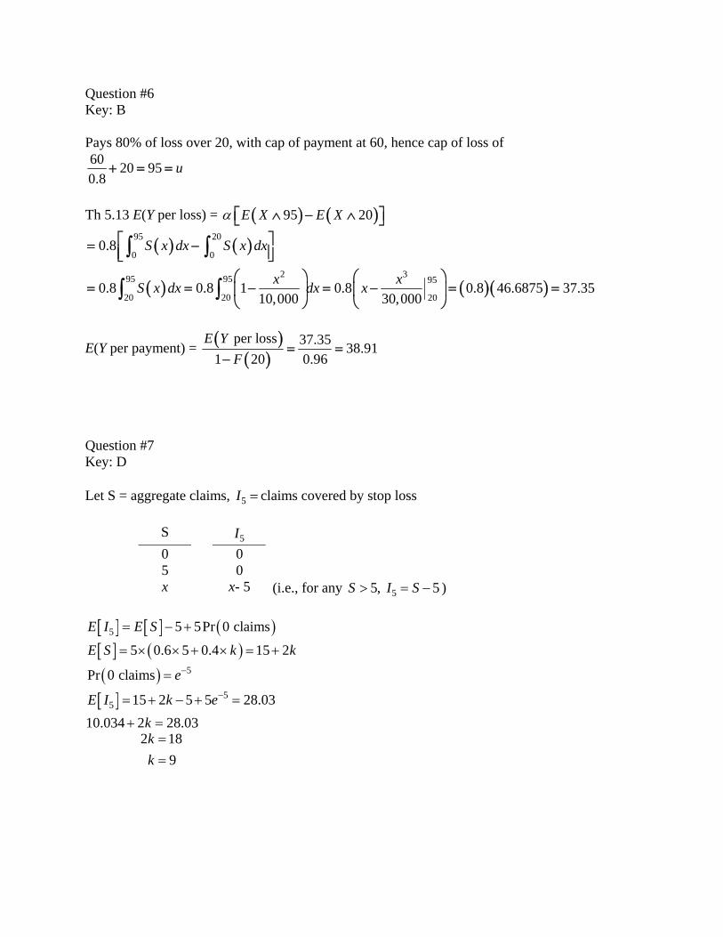
Question #6 Key: B Pays 80% of loss over 20, with cap of payment at 60, hence cap of loss of 60 20 950.8

u+ = =

Th 5.13 E(Y per loss) = ( ) ( )95 20E X E Xα ⎡ ⎤∧ − ∧⎣ ⎦

( ) ( )

( ) ( ) ( )

95 20

0 0

2 395 95 95

20 20 20

0.8

0.8 0.8 1 0.8 0.8 46.6875 37.3510,000 30,000

S x dx S x dx

x xS x dx dx x

⎡ ⎤= −⎢ ⎥⎣ ⎦⎛ ⎞ ⎛ ⎞

= = − = − = =⎜ ⎟ ⎜ ⎟⎝ ⎠ ⎝ ⎠

∫ ∫

∫ ∫

E(Y per payment) = ( )( )

per loss 37.35 38.911 20 0.96

E YF

= =−

Question #7 Key: D Let S = aggregate claims, 5I = claims covered by stop loss

S 5I 0 0 5 0 x x- 5 (i.e., for any 55, 5S I S> = − )

[ ] [ ] ( )5 5 5Pr 0 claimsE I E S= − +

[ ] ( )5 0.6 5 0.4 15 2E S k k= × × + × = +

( ) 5Pr 0 claims e−=

[ ] 55 15 2 5 5 28.03

10.034 2 28.03E I k e

k

−= + − + =

+ =

2 18

9kk==

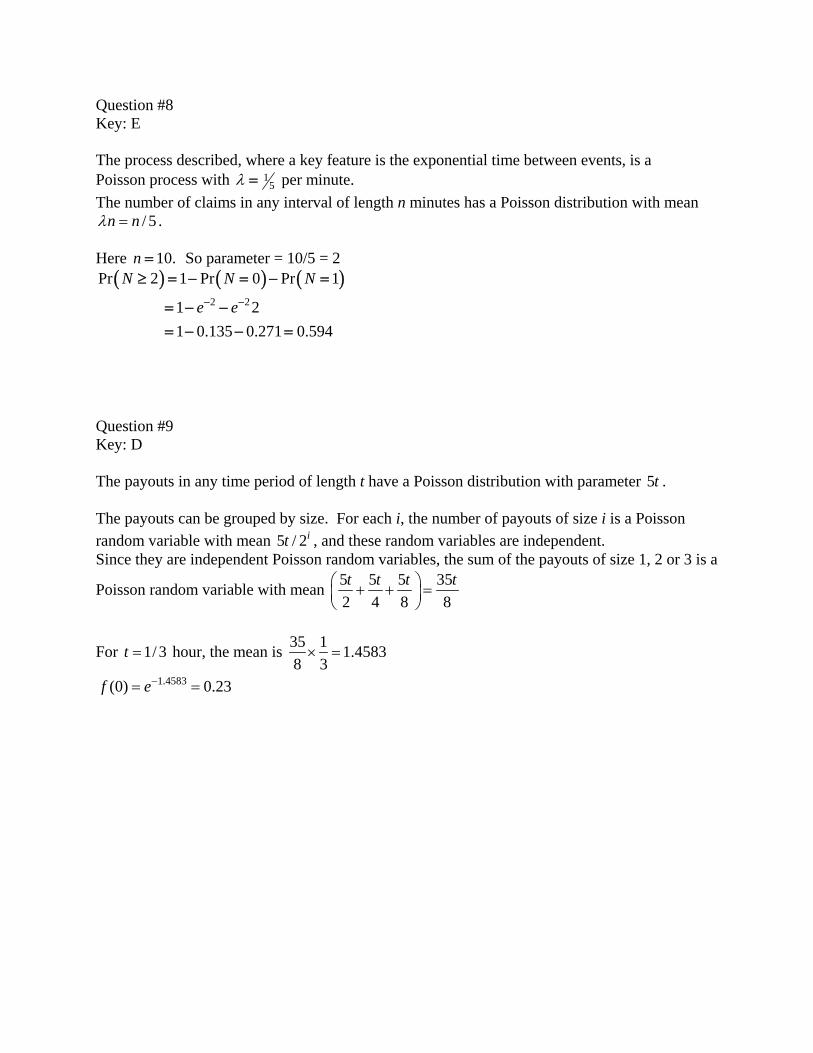
Question #8 Key: E The process described, where a key feature is the exponential time between events, is a Poisson process with 1

5λ = per minute. The number of claims in any interval of length n minutes has a Poisson distribution with mean

/ 5n nλ = . Here 10.n = So parameter = 10/5 = 2

( ) ( ) ( )2 2

Pr 2 1 Pr 0 Pr 1

1 21 0.135 0.271 0.594

N N N

e e− −

≥ = − = − =

= − −= − − =

Question #9 Key: D The payouts in any time period of length t have a Poisson distribution with parameter 5t . The payouts can be grouped by size. For each i, the number of payouts of size i is a Poisson random variable with mean 5 / 2it , and these random variables are independent. Since they are independent Poisson random variables, the sum of the payouts of size 1, 2 or 3 is a

Poisson random variable with mean 5 5 5 352 4 8 8t t t t⎛ ⎞+ + =⎜ ⎟

⎝ ⎠

For 1/ 3t = hour, the mean is 35 1 1.45838 3× =

1.4583(0) 0.23f e−= =

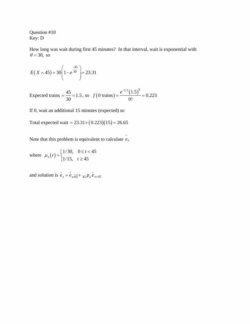
Question #10 Key: D How long was wait during first 45 minutes? In that interval, wait is exponential with

30,θ = so

( )45

3045 30 1 23.31E X e−⎛ ⎞

∧ = − =⎜ ⎟⎜ ⎟⎝ ⎠

Expected trains 45 1.530

= = , so ( ) ( )01.5 1.50 trains 0.223

0!e

f−

= =

If 0, wait an additional 15 minutes (expected) so Total expected wait ( )( )23.31 0.223 15 26.65= + =

Note that this problem is equivalent to calculate xeo

where ( )1/ 30, 0 451/15, 45x

tt

tμ

≤ <⎧= ⎨ ≥⎩

and solution is 45:45 45 xx x xe e p e += +o oo

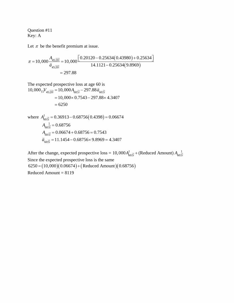
Question #11 Key: A Let π be the benefit premium at issue.

( )( )

45:20

45:20

0.20120 0.25634 0.43980 0.2563410,000 10,000

14.1121 0.25634 9.8969

297.88

Aa

π− +⎡ ⎤⎣ ⎦= =

−

=

&&

The expected prospective loss at age 60 is

15 45:20 60:5 60:510,000 10,000 297.88

10,000 0.7543 297.88 4.34076250

V A a= −

= × − ×=

&&

where ( )1

60:5 0.36913 0.68756 0.4398 0.06674A = − =

160:5 0.68756A =

60:5 0.06674 0.68756 0.7543A = + = 60:5 11.1454 0.68756 9.8969 4.3407a = − × =&& After the change, expected prospective loss = 1 1

60:5 60:510,000 (Reduced Amount) A A+ Since the expected prospective loss is the same

( )( ) ( )( )6250 10,000 0.06674 Reduced Amount 0.68756= + Reduced Amount = 8119

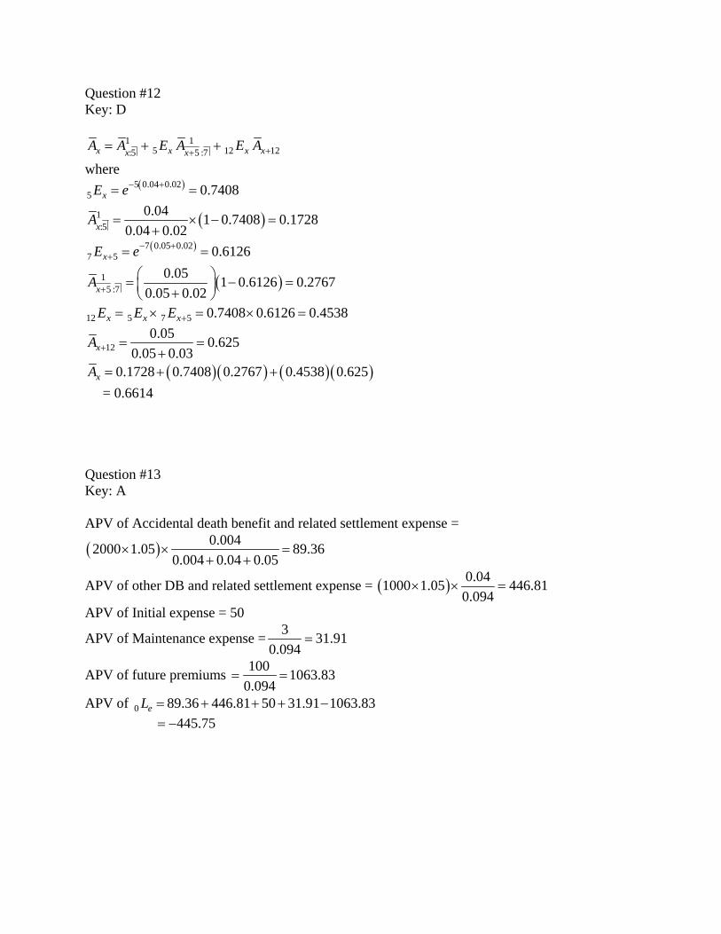
Question #12 Key: D

1 15 12 12:5 5 :7x x x xx xA A E A E A ++= + +

where ( )5 0.04 0.02

5 0.7408xE e− += =

( )1:5

0.04 1 0.7408 0.17280.04 0.02xA = × − =

+

( )7 0.05 0.027 5 0.6126xE e− +

+ = =

( )15 :7

0.05 1 0.6126 0.27670.05 0.02xA +

⎛ ⎞= − =⎜ ⎟+⎝ ⎠

12 5 7 5 0.7408 0.6126 0.4538x x xE E E += × = × =

120.05 0.625

0.05 0.03xA + = =+

( )( ) ( )( )0.1728 0.7408 0.2767 0.4538 0.625xA = + + = 0.6614 Question #13 Key: A APV of Accidental death benefit and related settlement expense =

( ) 0.0042000 1.05 89.360.004 0.04 0.05

× × =+ +

APV of other DB and related settlement expense = ( ) 0.041000 1.05 446.810.094

× × =

APV of Initial expense = 50

APV of Maintenance expense = 3 31.910.094

=

APV of future premiums 100 1063.830.094

= =

APV of 0 89.36 446.81 50 31.91 1063.83eL = + + + − 445.75= −

Question #14 Key: C Compute the probabilities of moving from healthy to NH. There are three paths. H to H to NH: (0.8)(0.05) = 0.04 H to HHC to NH: (0.15)(0.05) = 0.0075 H to NH to NH: (0.05)(1) = 0.05 Summing, we get 0.0975 as the probability for each member. Variance for m members = mpq, here = 50*(0.0975)(0.9025) = 4.40

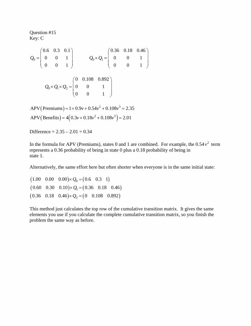
Question #15 Key: C

0

0.6 0.3 0.10 0 10 0 1

Q⎛ ⎞⎜ ⎟= ⎜ ⎟⎜ ⎟⎝ ⎠

0 1

0.36 0.18 0.460 0 10 0 1

Q Q⎛ ⎞⎜ ⎟× = ⎜ ⎟⎜ ⎟⎝ ⎠

0 1 2

0 0.108 0.8920 0 10 0 1

Q Q Q⎛ ⎞⎜ ⎟× × = ⎜ ⎟⎜ ⎟⎝ ⎠

( )( ) ( )

2 3

2 3

APV Premiums 1 0.9 0.54 0.108 2.35

APV Benefits 4 0.3 0.18 0.108 2.01

v v v

v v v

= + + + =

= + + =

Difference = 2.35 – 2.01 = 0.34 In the formula for APV (Premiums), states 0 and 1 are combined. For example, the 0.54 2v term represents a 0.36 probability of being in state 0 plus a 0.18 probability of being in state 1. Alternatively, the same effort here but often shorter when everyone is in the same initial state: ( ) ( )( ) ( )( ) ( )

0

1

2

1.00 0.00 0.00 0.6 0.3 1

0.60 0.30 0.10 0.36 0.18 0.46

0.36 0.18 0.46 0 0.108 0.892

Q

Q

Q

× =

× =

× =

This method just calculates the top row of the cumulative transition matrix. It gives the same elements you use if you calculate the complete cumulative transition matrix, so you finish the problem the same way as before.

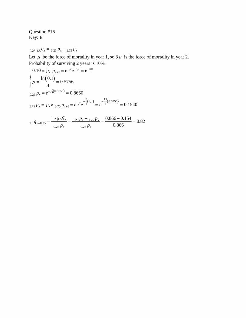
Question #16 Key: E

0.25 1.750.25 1.5 x x xq p p= −

Let μ be the force of mortality in year 1, so 3μ is the force of mortality in year 2. Probability of surviving 2 years is 10%

( )

3 410.10

ln 0.10.5756

4

x xp p e e eμ μ μ

μ

− − −+⎧ = = =

⎪⎨

= =⎪⎩

( )14 0.5756

0.25 0.8660xp e−= =

( ) ( )3 133 0.57564 4

1.75 0.75 1 0.1540x x xp p p e e eμμ − −−

+= × = = =

0.251.5 0.25 1.751.5 0.25

0.25 0.25

0.866 0.154 0.820.866

x x xx

x x

q p pqp p+

− −= = = =

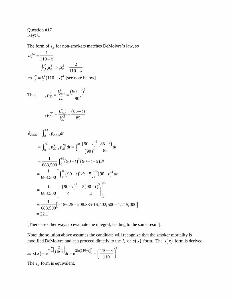
Question #17 Key: C The form of xl for non-smokers matches DeMoivre’s law, so

1110

NSx x

μ =−

212 110

S Sx x x

μ μ= ⇒ =−

( )20 110S S

xl l x⇒ = − [see note below]

Thus ( )220

20 220

9090

SS t

t Stlp

l+ −

= =

( )2525

25

8585

NSNS t

t NStlp

l+ −

= =

( )( )

( )

( ) ( )

8520:25 20:250

285 85

20 25 20 0

85 2

0

90 858590

1 90 90 5688,500

t

S NSt t

e p dt

t tp p dt dt

t t dt

=

− −= =

= − − −

∫

∫ ∫

∫

o

( ) ( )85 853 2

0 0

1 90 5 90688,500

t dt t dt⎡= − − −⎢⎣∫ ∫

( ) ( )854 3

0

90 5 901688,500 4 3

t t⎡ ⎤− − −= +⎢ ⎥

⎢ ⎥⎣ ⎦

[ ]1 156.25 208.33 16,402,500 1,215,000688,500

= − + + −

= 22.1 [There are other ways to evaluate the integral, leading to the same result]. Note: the solution above assumes the candidate will recognize that the smoker mortality is modified DeMoivre and can proceed directly to the xl or ( )s x form. The ( )s x form is derived

as ( ) ( )0 0

222ln 110110 110

110

x xtt xs x e dt e

⎛ ⎞⎜ ⎟⎝ ⎠

− −− −⎛ ⎞= = = ⎜ ⎟⎝ ⎠

∫

The xl form is equivalent.

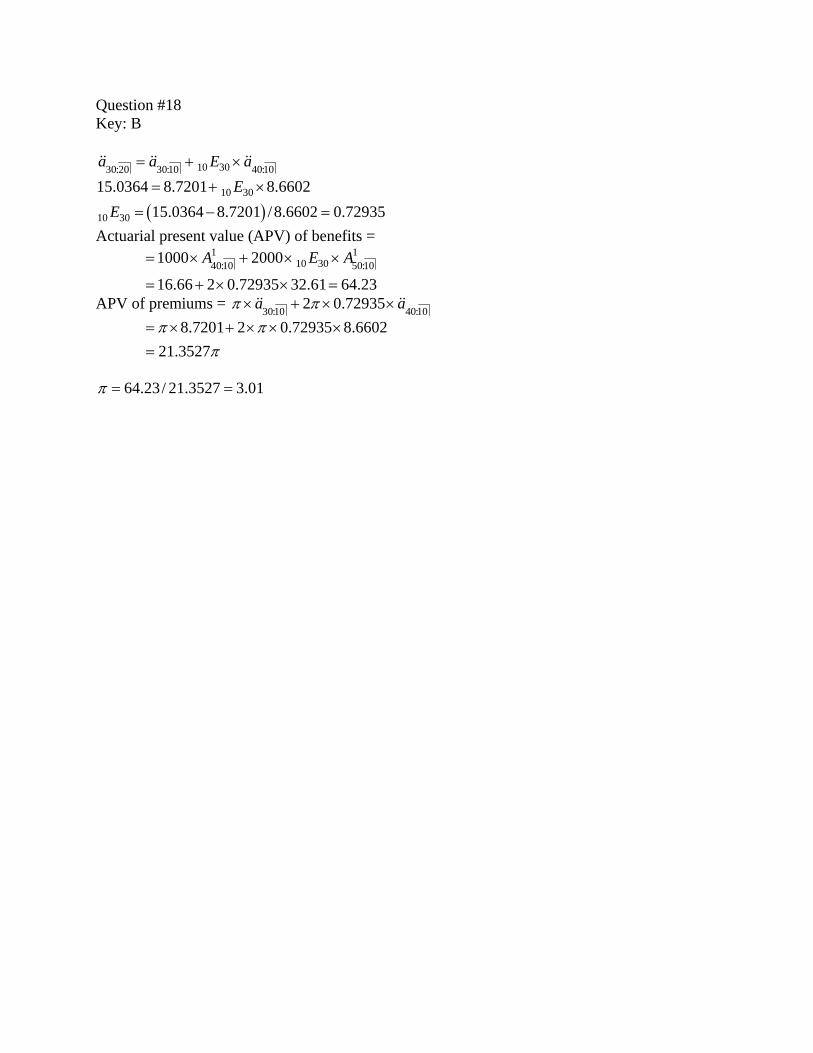
Question #18 Key: B

10 3030:20 30:10 40:10a a E a= + ×&& && &&

10 3015.0364 8.7201 8.6602E= + ×

( )10 30 15.0364 8.7201 /8.6602 0.72935E = − = Actuarial present value (APV) of benefits =

1 1

10 3040:10 50:101000 2000

16.66 2 0.72935 32.61 64.23

A E A= × + × ×

= + × × =

APV of premiums = 30:10 40:102 0.72935a aπ π× + × ×&& &&

8.7201 2 0.72935 8.6602

21.3527π π

π= × + × × ×=

64.23/ 21.3527 3.01π = =

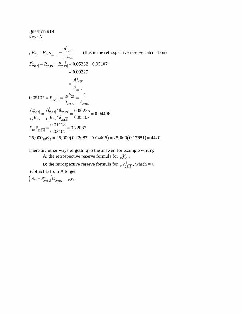
Question #19 Key: A

125:15

15 25 25 25:1515 25

(this is the retrospective reserve calculation)A

V P sE

= −&&

1 125:15 25:15 25:15

125:15

25:15

0.05332 0.05107

0.00225

P P P

Aa

= − = −

=

=&&

1 15 2525:15

25:15 25:15

10.05107 EPa s

= = =&& &&

1125:15 25:15 25:15

15 25 15 25 25:15

/ 0.00225 0.04406/ 0.05107

A A aE E a

= = =&&

&&

25 25:150.01128 0.220870.05107

P s = =&&

( ) ( )15 2525,000 25,000 0.22087 0.04406 25,000 0.17681 4420V = − = = There are other ways of getting to the answer, for example writing

A: the retrospective reserve formula for 15 25V .

B: the retrospective reserve formula for 115 25:15V , which = 0

Subtract B from A to get

( )125 15 2525:15 25:15P P s V− =&&

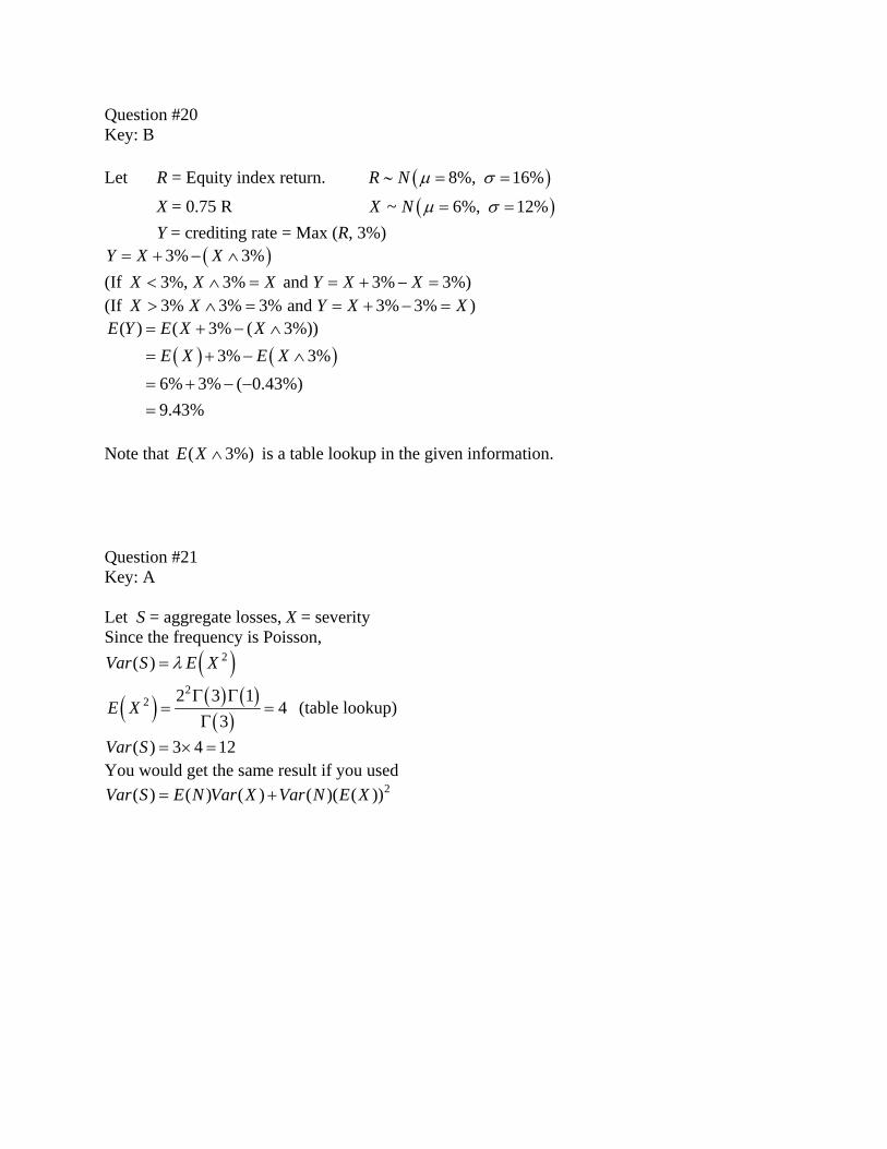
Question #20 Key: B Let R = Equity index return. ( )8%, 16%R N μ σ∼ = =

X = 0.75 R ( )~ 6%, 12%X N μ σ= = Y = crediting rate = Max (R, 3%)

( )3% 3%Y X X= + − ∧ (If 3%, 3% and 3% 3%)X X X Y X X< ∧ = = + − = (If 3% 3% 3% and 3% 3% )X X Y X X> ∧ = = + − =

( ) ( )( ) ( 3% ( 3%))

3% 3%6% 3% ( 0.43%)9.43%

E Y E X XE X E X

= + − ∧

= + − ∧

= + − −=

Note that ( 3%)E X ∧ is a table lookup in the given information. Question #21 Key: A Let S = aggregate losses, X = severity Since the frequency is Poisson,

( )2( )Var S E Xλ=

( ) ( ) ( )( )

22 2 3 1

43

E XΓ Γ

= =Γ

(table lookup)

( ) 3 4 12Var S = × = You would get the same result if you used

2( ) ( ) ( ) ( )( ( ))Var S E N Var X Var N E X= +

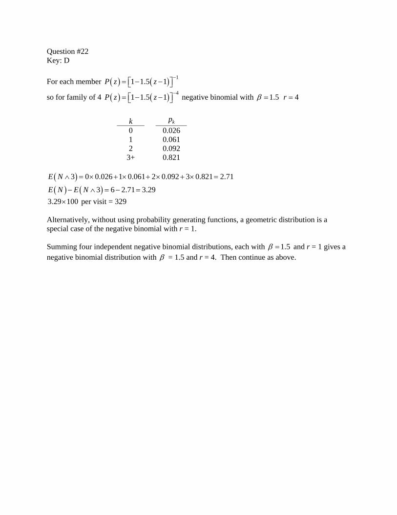
Question #22 Key: D For each member ( ) ( ) 11 1.5 1P z z −

= − −⎡ ⎤⎣ ⎦

so for family of 4 ( ) ( ) 41 1.5 1P z z −= − −⎡ ⎤⎣ ⎦ negative binomial with 1.5β = 4r =

k kp 0 0.026 1 0.061 2 0.092

3+ 0.821 ( )( ) ( )

3 0 0.026 1 0.061 2 0.092 3 0.821 2.71

3 6 2.71 3.29

E N

E N E N

∧ = × + × + × + × =

− ∧ = − =

3.29 100× per visit = 329 Alternatively, without using probability generating functions, a geometric distribution is a special case of the negative binomial with r = 1. Summing four independent negative binomial distributions, each with 1.5β = and r = 1 gives a negative binomial distribution with β = 1.5 and r = 4. Then continue as above.

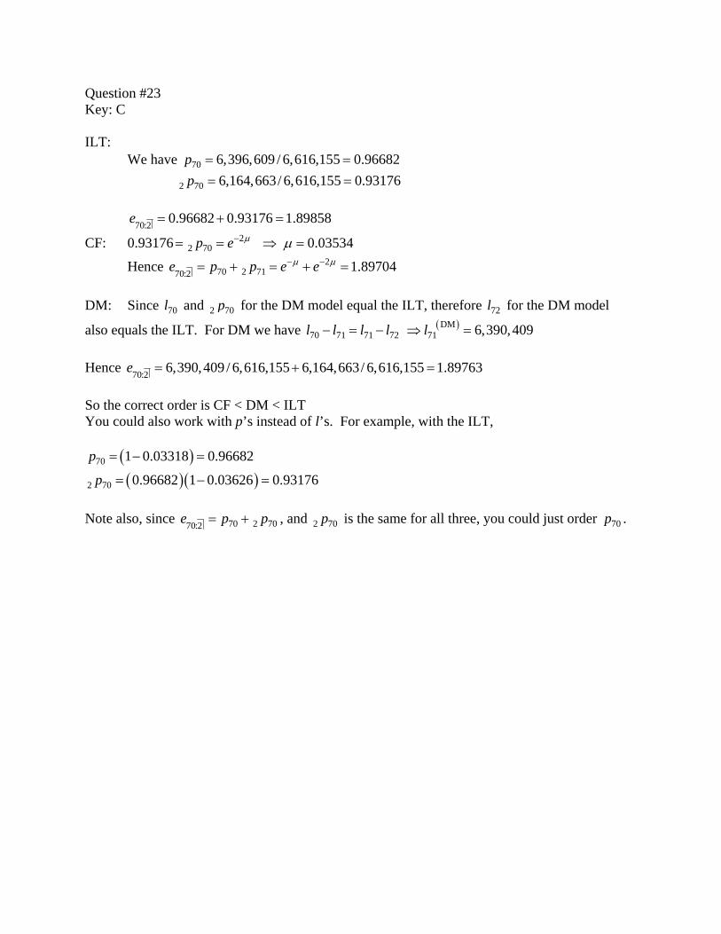
Question #23 Key: C ILT: We have 70 6,396,609 / 6,616,155 0.96682p = = 2 70 6,164,663/ 6,616,155 0.93176p = = 70:2 0.96682 0.93176 1.89858e = + =

CF: 0.93176 22 70 0.03534p e μ μ−= = ⇒ =

Hence 270 2 7170:2 1.89704e p p e eμ μ− −= + = + =

DM: Since 70l and 2 70p for the DM model equal the ILT, therefore 72l for the DM model

also equals the ILT. For DM we have ( )DM70 71 71 72 71 6,390,409l l l l l− = − ⇒ =

Hence 70:2 6,390,409 / 6,616,155 6,164,663/ 6,616,155 1.89763e = + = So the correct order is CF < DM < ILT You could also work with p’s instead of l’s. For example, with the ILT,

( )( )( )

70

2 70

1 0.03318 0.96682

0.96682 1 0.03626 0.93176

p

p

= − =

= − =

Note also, since 70 2 7070:2e p p= + , and 2 70p is the same for all three, you could just order 70p .

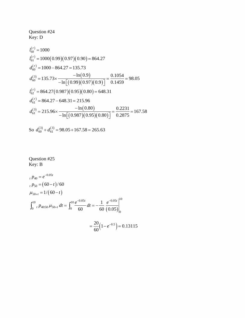
Question #24 Key: D ( )60 1000l τ = ( ) ( )( )( )( )

61

60

1000 0.99 0.97 0.90 864.27

1000 864.27 135.73

l

d

τ

τ

= =

= − =

( ) ( )( )( )( )

360

ln 0.9 0.1054135.73 98.05ln 0.99 0.97 0.9 0.1459

d−

= × = =− ⎡ ⎤⎣ ⎦

( ) ( )( )( )( )

62

61

864.27 0.987 0.95 0.80 648.31

864.27 648.31 215.96

l

d

τ

τ

= =

= − =

( ) ( )( )( )( )

361

ln 0.80 0.2231215.96 167.58ln 0.987 0.95 0.80 0.2875

d−

= × = =− ⎡ ⎤⎣ ⎦

So ( ) ( )3 3

60 61 98.05 167.58 265.63d d+ = + = Question #25 Key: B

0.0540

tt p e−=

( )( )

50

50

60 / 60

1/ 60t

t

p t

tμ +

= −

= −

( )

100.05 0.0510 1040:50 500 0

0

160 60 0.05

t t

t te ep dt dtμ− −

+ = = −∫ ∫

( )0.520 1 0.1311560

e−= − =

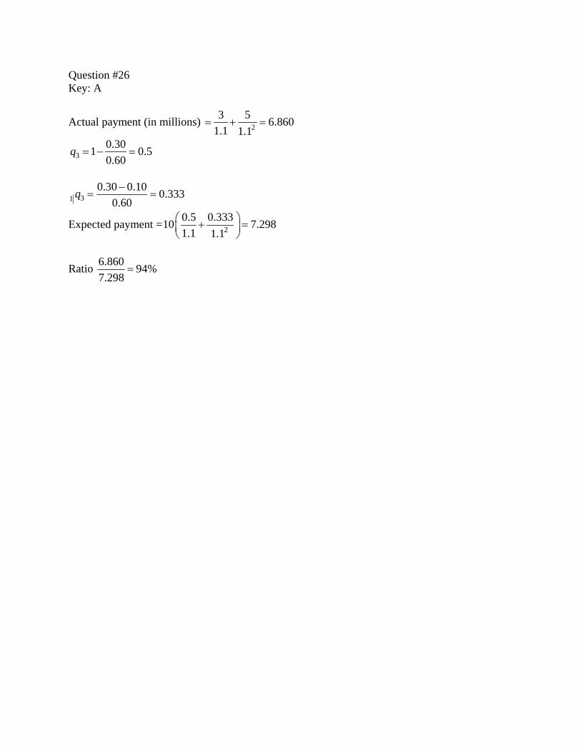
Question #26 Key: A

Actual payment (in millions) 23 5 6.860

1.1 1.1= + =

30.301 0.50.60

q = − =

310.30 0.10 0.333

0.60q −

= =

Expected payment = 20.5 0.33310 7.2981.1 1.1

⎛ ⎞+ =⎜ ⎟⎝ ⎠

Ratio 6.860 94%7.298

=

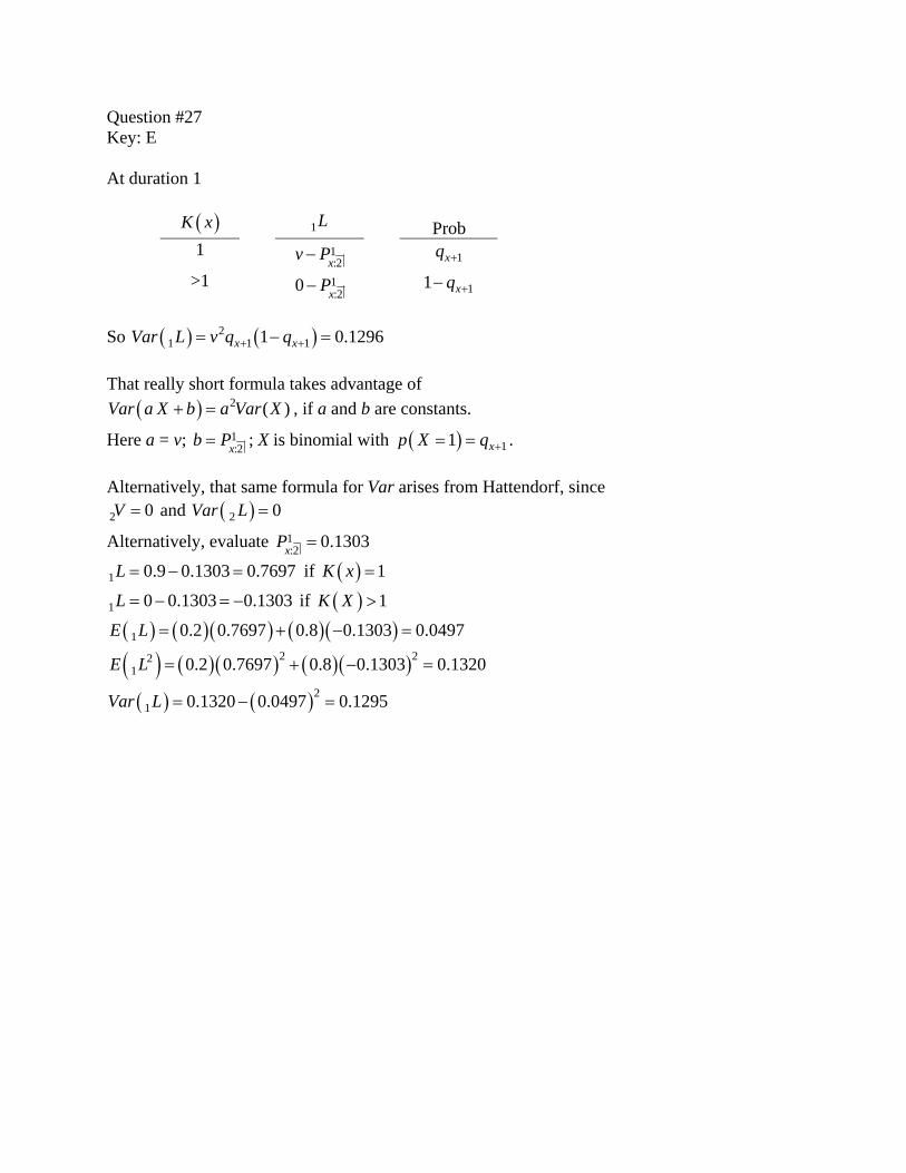
Question #27 Key: E At duration 1

( )K x 1L Prob 1 1

:2xv P− 1xq +

>1 1:20 xP− 11 xq +−

So ( ) ( )2

1 1 11 0.1296x xVar L v q q+ += − = That really short formula takes advantage of

( ) 2 ( )Var a X b a Var X+ = , if a and b are constants.

Here a = v; 1:2xb P= ; X is binomial with ( ) 11 xp X q += = .

Alternatively, that same formula for Var arises from Hattendorf, since 2 0V = and ( )2 0Var L =

Alternatively, evaluate 1:2 0.1303xP =

1 0.9 0.1303 0.7697L = − = if ( ) 1K x =

1 0 0.1303 0.1303L = − = − if ( ) 1K X >

( ) ( )( ) ( )( )1 0.2 0.7697 0.8 0.1303 0.0497E L = + − =

( ) ( )( ) ( )( )2 221 0.2 0.7697 0.8 0.1303 0.1320E L = + − =

( ) ( )21 0.1320 0.0497 0.1295Var L = − =

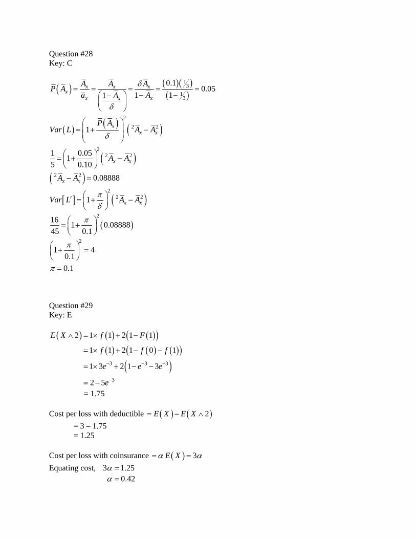
Question #28 Key: C

( ) ( )( )( )

13

13

0.10.05

1 11x x x

xx xx

A A AP Aa AA

δ

δ

= = = = =⎛ ⎞ − −−⎜ ⎟⎝ ⎠

( ) ( ) ( )2

2 21 xx x

P AVar L A A

δ

⎛ ⎞⎜ ⎟= + −⎜ ⎟⎝ ⎠

( )2

2 21 0.0515 0.10 x xA A⎛ ⎞= + −⎜ ⎟

⎝ ⎠

( )2 2 0.08888x xA A− =

[ ] ( )2

2 21 x xVar L A Aπδ

⎛ ⎞′ = + −⎜ ⎟⎝ ⎠

( )216 1 0.08888

45 0.1π⎛ ⎞= +⎜ ⎟

⎝ ⎠

2

1 40.10.1

π

π

⎛ ⎞+ =⎜ ⎟⎝ ⎠=

Question #29 Key: E ( ) ( ) ( )( )

( ) ( ) ( )( )( )3 3 3

3

2 1 1 2 1 1

1 1 2 1 0 1

1 3 2 1 3

2 5

E X f F

f f f

e e e

e

− − −

−

∧ = × + −

= × + − −

= × + − −

= −

= 1.75 Cost per loss with deductible ( ) ( )2E X E X= − ∧ = 3 – 1.75 = 1.25 Cost per loss with coinsurance ( ) 3E Xα α= = Equating cost, 3 1.25α = 0.42α =

Question #30 Key: A Let N be the number of clubs accepted X be the number of members of a selected club S be the total persons appearing N is binomial with m = 1000 q = 0.20 ( ) ( )( )1000 0.20 200E N = =

( ) ( )( )( )1000 0.20 0.80 160Var N = = ( ) ( ) ( ) ( )( )200 20 4000E S E N E X= = =

( ) ( ) ( ) ( ) ( )

( )( ) ( )( )

2

2200 20 160 2068,000

Var S E N Var X Var N E X= + ⎡ ⎤⎣ ⎦

= +

=

Budget ( )10 10 ( )E S Var S= × + ×

10 4000 10 68,00042,610

= × + ×=

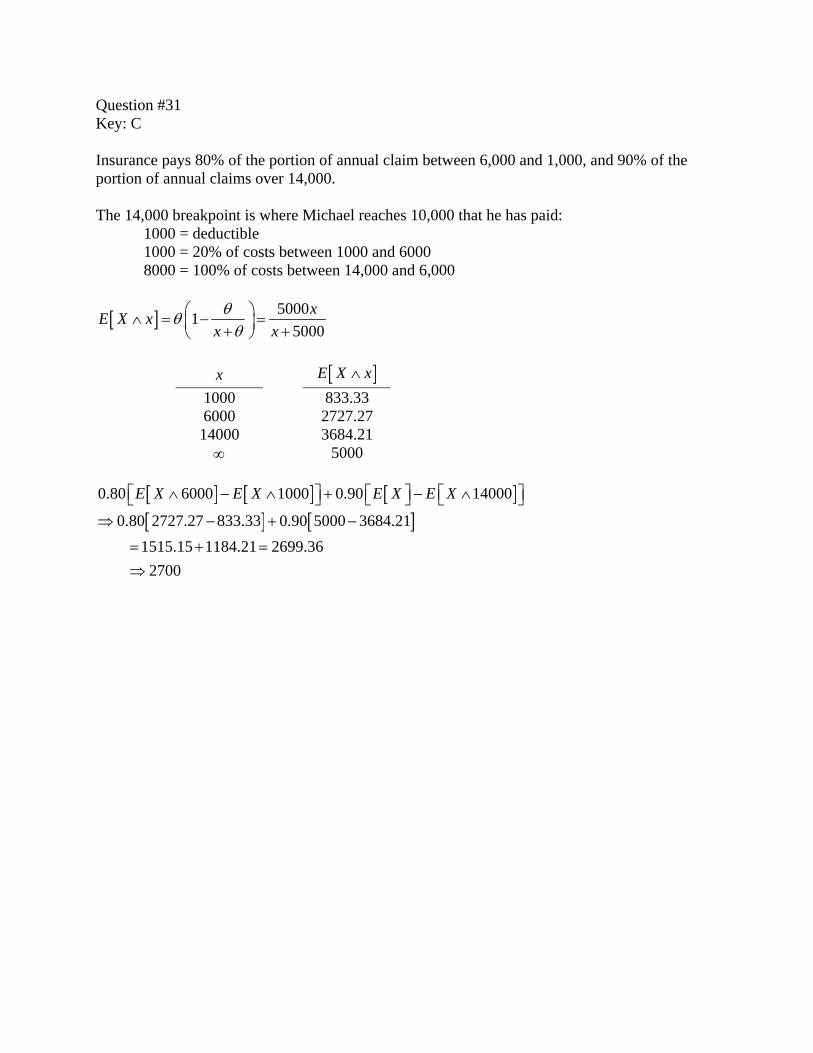
Question #31 Key: C Insurance pays 80% of the portion of annual claim between 6,000 and 1,000, and 90% of the portion of annual claims over 14,000. The 14,000 breakpoint is where Michael reaches 10,000 that he has paid: 1000 = deductible 1000 = 20% of costs between 1000 and 6000 8000 = 100% of costs between 14,000 and 6,000

[ ] 500015000

xE X xx xθθθ

⎛ ⎞∧ = − =⎜ ⎟+ +⎝ ⎠

x [ ]E X x∧

1000 833.33 6000 2727.27 14000 3684.21 ∞ 5000

[ ] [ ] [ ]0.80 6000 1000 0.90 14000E X E X E X E X⎡ ⎤ ⎡ ⎤ ⎡ ⎤∧ − ∧ + − ∧⎣ ⎦ ⎣ ⎦ ⎣ ⎦

[ ] [ ]0.80 2727.27 833.33 0.90 5000 3684.211515.15 1184.21 2699.36

2700

⇒ − + −

= + =⇒

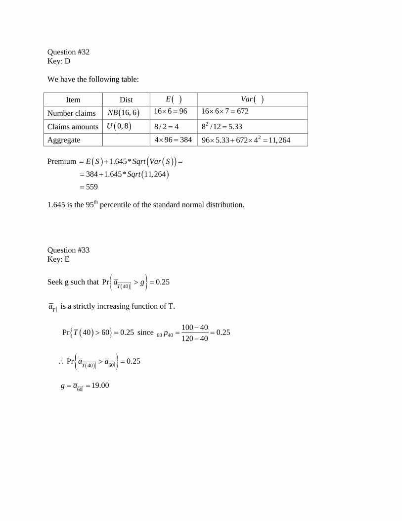
Question #32 Key: D We have the following table:

Item Dist ( )E ( )Var

Number claims ( )16, 6NB 16 6 96× = 16 6 7 672× × =

Claims amounts ( )0, 8U 8 / 2 4= 28 /12 5.33=

Aggregate 4 96 384× = 296 5.33 672 4 11,264× + × = Premium ( ) ( )( )1.645*E S Sqrt Var S= + =

( )384 1.645* 11,264559

Sqrt= +

=

1.645 is the 95th percentile of the standard normal distribution. Question #33 Key: E

Seek g such that ( ){ }40Pr 0.25

Ta g> =

Ta is a strictly increasing function of T.

( ){ }Pr 40 60 0.25T > = since 60 40100 40 0.25120 40

p −= =

−

( ){ }6040Pr 0.25

Ta a∴ > =

60 19.00g a= =

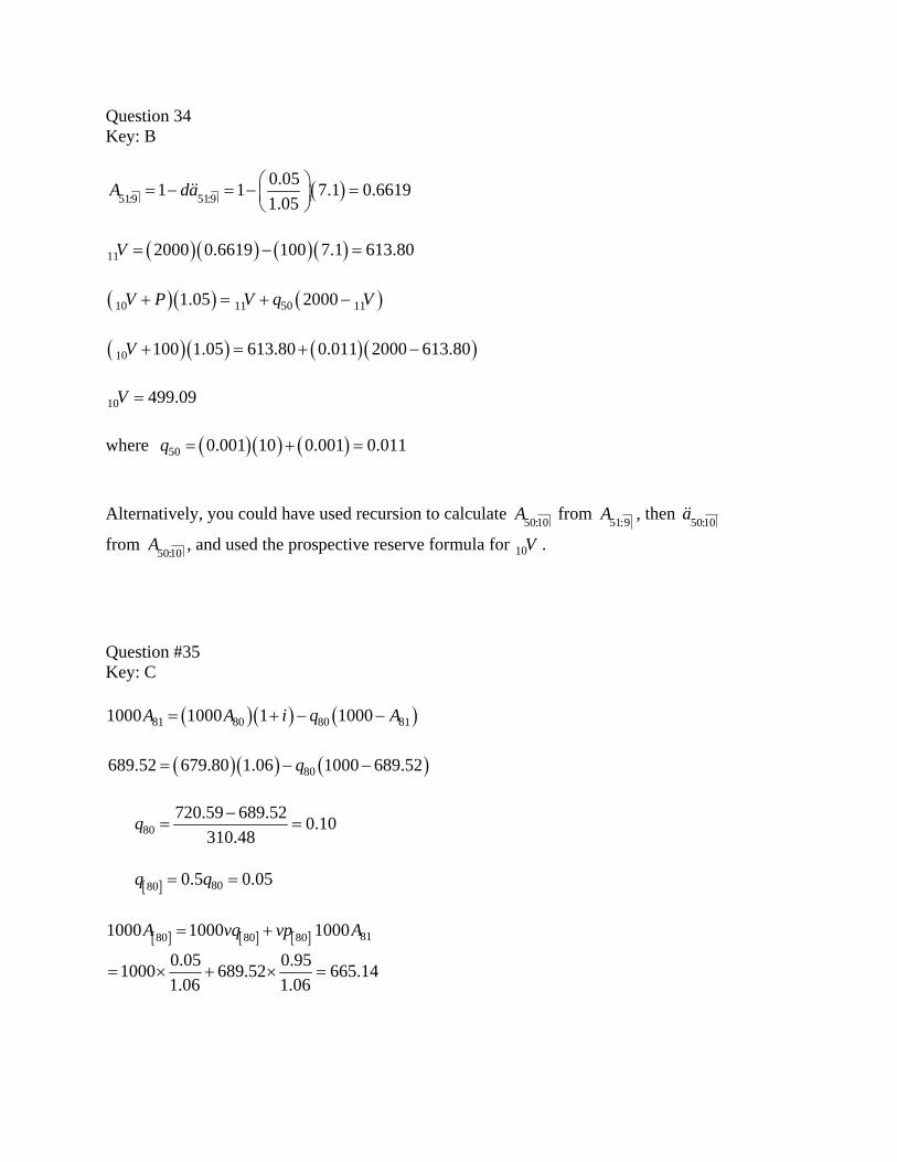
Question 34 Key: B

( )51:9 51:90.051 1 7.1 0.66191.05

A da ⎛ ⎞= − = − =⎜ ⎟⎝ ⎠

&&

( )( ) ( )( )11 2000 0.6619 100 7.1 613.80V = − =

( )( ) ( )10 11 50 111.05 2000V P V q V+ = + − ( )( ) ( )( )10 100 1.05 613.80 0.011 2000 613.80V + = + − 10 499.09V = where ( )( ) ( )50 0.001 10 0.001 0.011q = + = Alternatively, you could have used recursion to calculate 50:10A from 51:9A , then 50:10a&&

from 50:10A , and used the prospective reserve formula for 10V . Question #35 Key: C

( )( ) ( )81 80 80 811000 1000 1 1000A A i q A= + − −

( )( ) ( )80689.52 679.80 1.06 1000 689.52q= − −

80720.59 689.52 0.10

310.48q −

= =

[ ] 8080 0.5 0.05q q= =

[ ] [ ] [ ] 8180 80 801000 1000 1000A vq vp A= +

0.05 0.951000 689.52 665.141.06 1.06

= × + × =

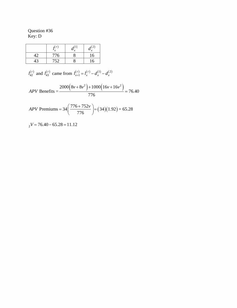
Question #36 Key: D

( )xlτ ( )1

xd ( )2xd

42 776 8 16 43 752 8 16

( )42l τ and ( )

43l τ came from ( ) ( ) ( ) ( )1 21x x x xl l d dτ τ+ = − −

( ) ( )2 22000 8 8 1000 16 16Benefits = 76.40

776

v v v vAPV

+ + +=

( )( )776 752Premiums 34 34 1.92776

vAPV +⎛ ⎞= =⎜ ⎟⎝ ⎠

= 65.28

2 76.40 65.28 11.12V = − =

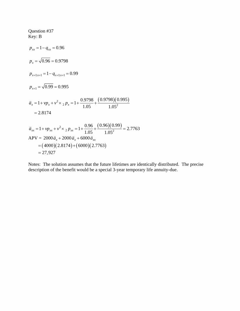
Question #37 Key: B

1 0.96xx xxp q= − =

0.96 0.9798xp = =

1: 1 1: 11 0.99x x x xp q+ + + += − =

1 0.99 0.995xp + = =

( )( )22 2

0.9798 0.9950.97981 11.05 1.05

2.8174

x x xa vp v p= + + × = + +

=

&&

( )( )2

2 20.96 0.990.961 1 2.7763

1.05 1.05xx xx xxa vp v p= + + × = + + =&&

APV = 2000 2000 6000x x xxa a a+ +&& && && ( )( ) ( )( )4000 2.8174 6000 2.7763= + 27,927= Notes: The solution assumes that the future lifetimes are identically distributed. The precise description of the benefit would be a special 3-year temporary life annuity-due.

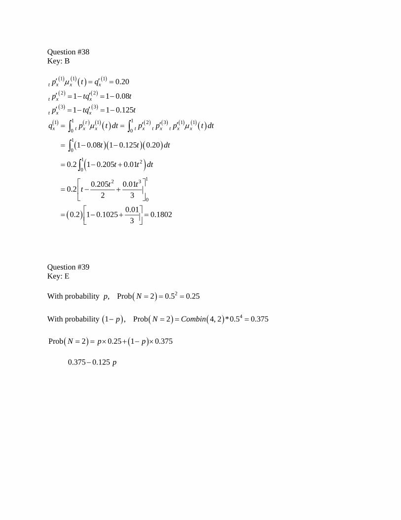
Question #38 Key: B

( ) ( ) ( ) ( )1 1 1 0.20t x x xp t qμ′ ′= = ( ) ( )2 21 1 0.08t x xp tq t′ ′= − = − ( ) ( )3 31 1 0.125t x xp tq t′ ′= − = −

( ) ( ) ( ) ( ) ( ) ( ) ( ) ( ) ( )

( )( )( )

( )

( )

1 11 1 2 3 1 10 0

1

0

1 20

12 3

0

1 0.08 1 0.125 0.20

0.2 1 0.205 0.01

0.205 0.010.22 3

0.010.2 1 0.1025 0.18023

x t x x t x t x t x xq p t dt p p p t dt

t t dt

t t dt

t tt

τ μ μ′ ′ ′= =

= − −

= − +

⎡ ⎤= − +⎢ ⎥

⎣ ⎦

⎡ ⎤= − + =⎢ ⎥⎣ ⎦

∫ ∫

∫

∫

Question #39 Key: E With probability ( ) 2, Prob 2 0.5 0.25p N = = = With probability ( ) ( ) ( ) 41 , Prob 2 4, 2 *0.5 0.375p N Combin− = = =

( ) ( )Prob 2 0.25 1 0.375N p p= = × + − × 0.375 0.125 p−

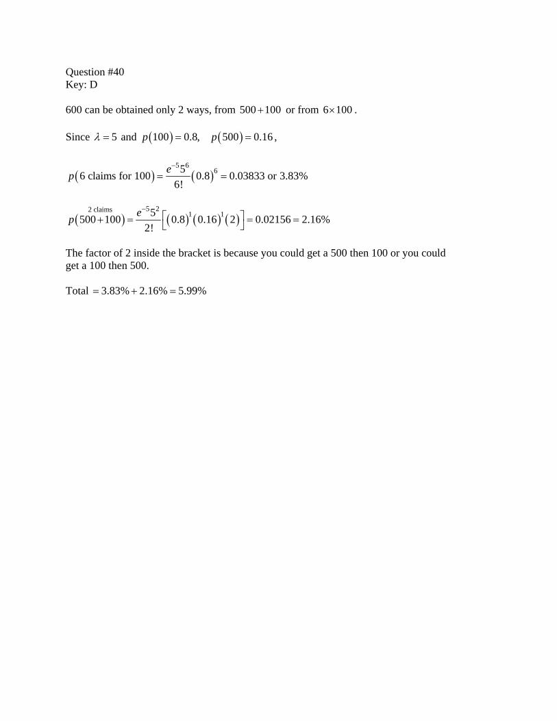
Question #40 Key: D 600 can be obtained only 2 ways, from 500 100+ or from 6 100× . Since 5λ = and ( ) ( )100 0.8, 500 0.16p p= = ,

( ) ( )5 6

656 claims for 100 0.8 0.03833 or 3.83%6!

ep−

= =

( ) ( ) ( ) ( )5 22 claims 1 15500 100 0.8 0.16 2 0.02156 2.16%2!

ep−

⎡ ⎤+ = = =⎣ ⎦

The factor of 2 inside the bracket is because you could get a 500 then 100 or you could get a 100 then 500. Total 3.83% 2.16% 5.99%= + =