MDX (Multi-Dimensional eXpressions) is a query language used to retrieve data from multi-dimensional databases.

MDX was originally designed by Microsoft and introduced along with Analysis Services 7.0 in 1998.

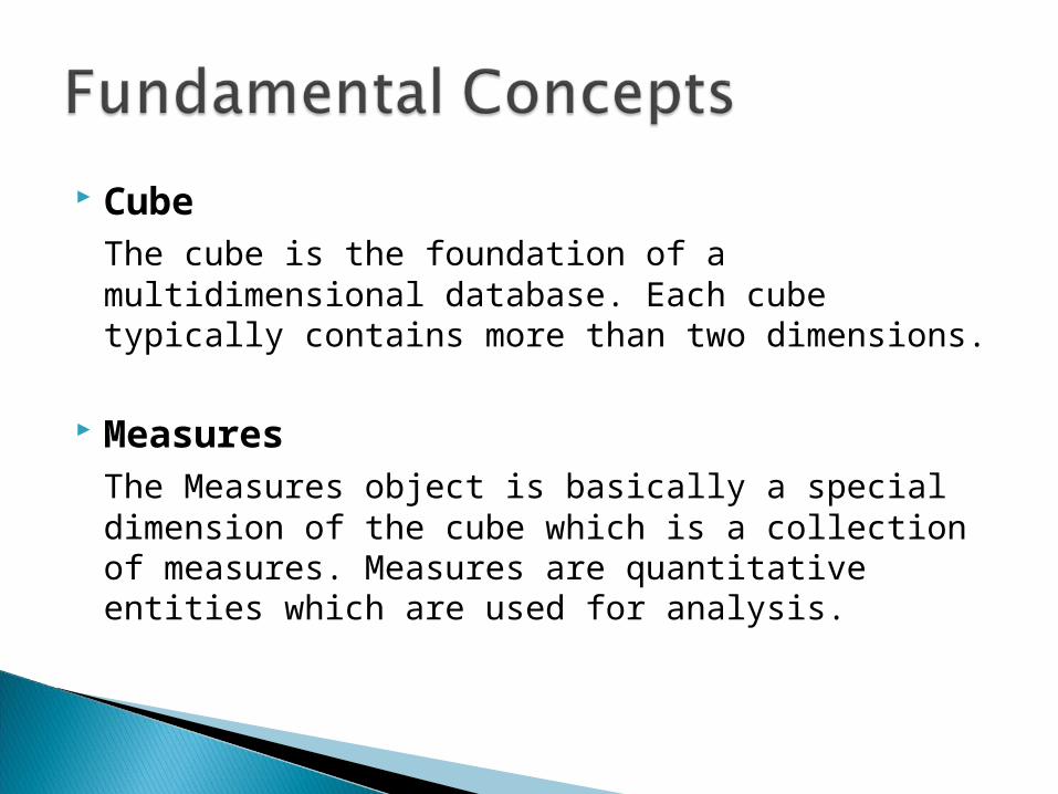
CubeThe cube is the foundation of a multidimensional database. Each cube typically contains more than two dimensions.

MeasuresThe Measures object is basically a special dimension of the cube which is a collection of measures. Measures are quantitative entities which are used for analysis.

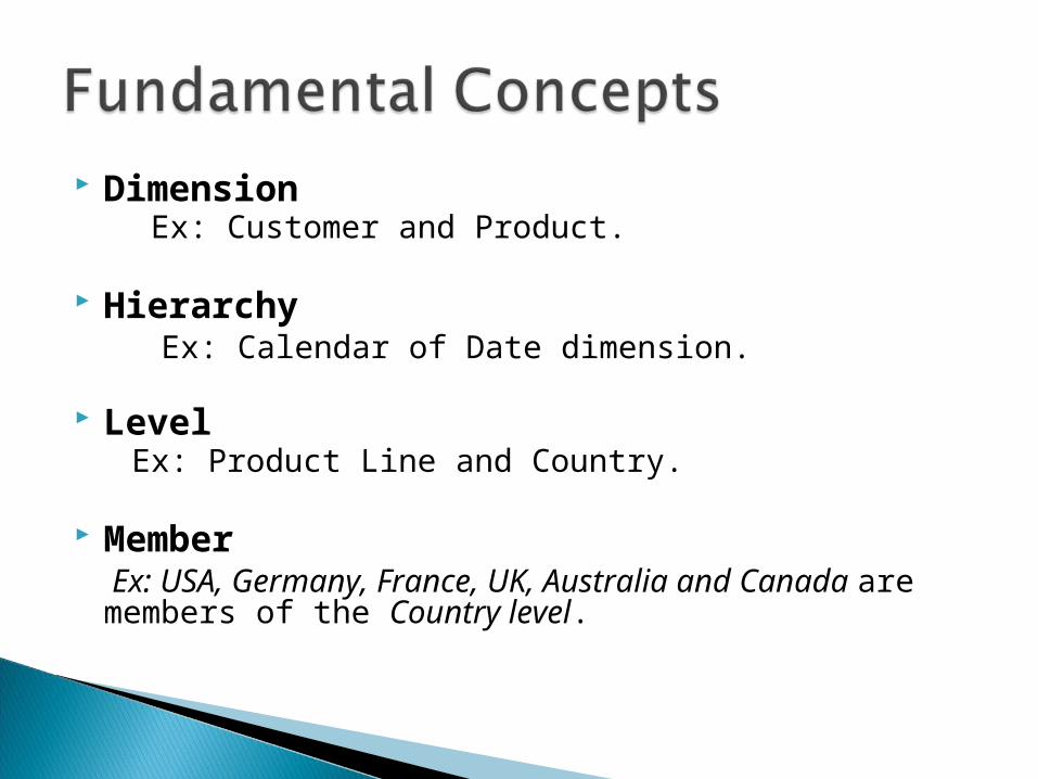
Dimension Ex: Customer and Product.

Hierarchy Ex: Calendar of Date dimension.

Level Ex: Product Line and Country.

Member Ex: USA, Germany, France, UK, Australia and Canada

are members of the Country level.

you can use the following format for accessing a member:

[DimensionName].[HierarchyName]. [LevelName].[MemberName]

Ex: [Customer].[Country].Australia

Let’s start to build our first MDX query. The basic MDX query has the following structure:

SELECT axisA1,……, axisAn ON COLUMNS,

axisB1,……, axisBn ON ROWS

FROM cube Let’s compare that to the similar SQL

statement: SELECT column1, column2, …, columnn

FROM table

SELECT Measures.[Internet Sales Amount] on

COLUMNS, {[Customer].[Country].[France], [Customer].[Country].[Germany], [Customer].[Country].[United Kingdom]}

on ROWS FROM [Adventure Works]

Country Internet Sales Amount

France 120,000

Germany 999,999

United Kingdom 55,000

SELECT Measures.[Sales] ON COLUMS

FROM ProductsCube

WHERE ([Product].[Color].[Silver])

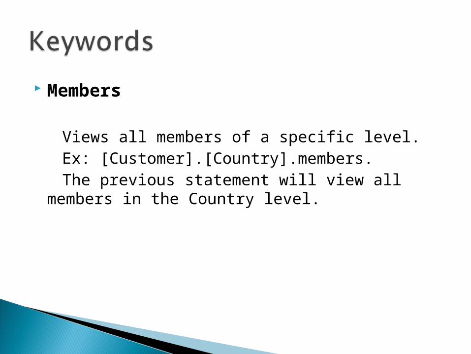
Members Views all members of a specific level. Ex: [Customer].[Country].members. The previous statement will view all members in

the Country level.

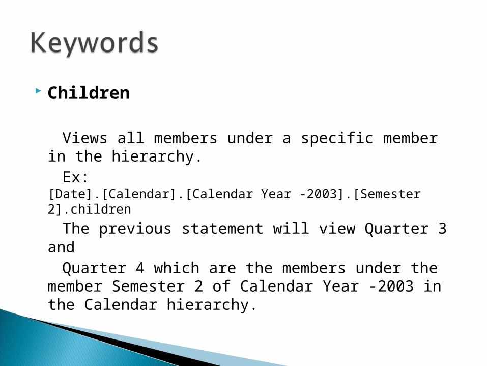
Children Views all members under a specific member in

the hierarchy. Ex: [Date].[Calendar].

[Calendar Year -2003].[Semester 2].children

The previous statement will view Quarter 3 and Quarter 4 which are the members under the

member Semester 2 of Calendar Year -2003 in the Calendar hierarchy.

Named Sets: SELECT Measures.[Internet Sales Amount]

on COLUMNS, {[Customer].[Country].[France], [Customer].[Country].[Germany], [Customer].[Country].[United Kingdom]}

on ROWS FROM [Adventure Works]

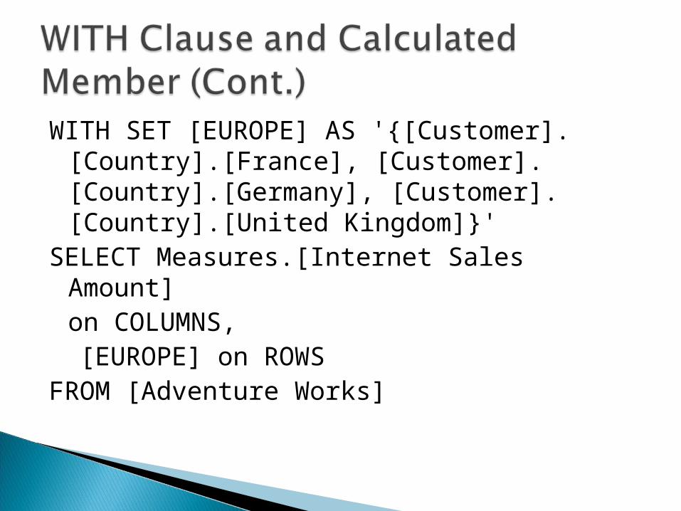
WITH SET [EUROPE] AS '{[Customer].[Country].[France], [Customer].[Country].[Germany], [Customer].[Country].[United Kingdom]}'

SELECT Measures.[Internet Sales Amount] on COLUMNS,

[EUROPE] on ROWS FROM [Adventure Works]

Calculated Members:

WITH MEMBER [MEASURES].[Profit] AS ([Measures].[Internet Sales Amount] - [Measures].[Total Product Cost]) SELECT [MEASURES].[Profit] ON COLUMNS, [Customer].[Country].MEMBERS ON ROWS FROM [Adventure Works]

2008/2/14 17

A data warehouse is a subject-oriented, integrated, time-variant, and nonvolatile collection of data in support of management’s decision-making process.

2008/2/14 18

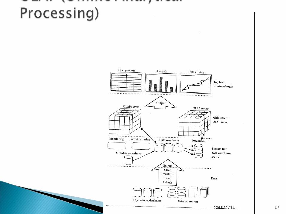
An OLAP system manages large amount of historical data, provides facilities for summarization and aggregation, and stores and manages information at different levels of granularity.

2008/2/14 19

High performance for both systems◦ DBMS— tuned for OLTP: access methods,

indexing, concurrency control, recovery◦ Warehouse—tuned for OLAP: complex OLAP

queries, multidimensional view, consolidation. Different functions and different data:

◦ missing data: Decision support requires historical data which operational DBs do not typically maintain

◦ data consolidation: DS requires consolidation (aggregation, summarization) of data from heterogeneous sources

◦ data quality: different sources typically use inconsistent data representations, codes and formats which have to be reconciled

2008/2/14 20

A data warehouse is based on a multidimensional data model which views data in the form of a data cube.

A data cube, such as sales, allows data to be modeled and viewed in multiple dimensions

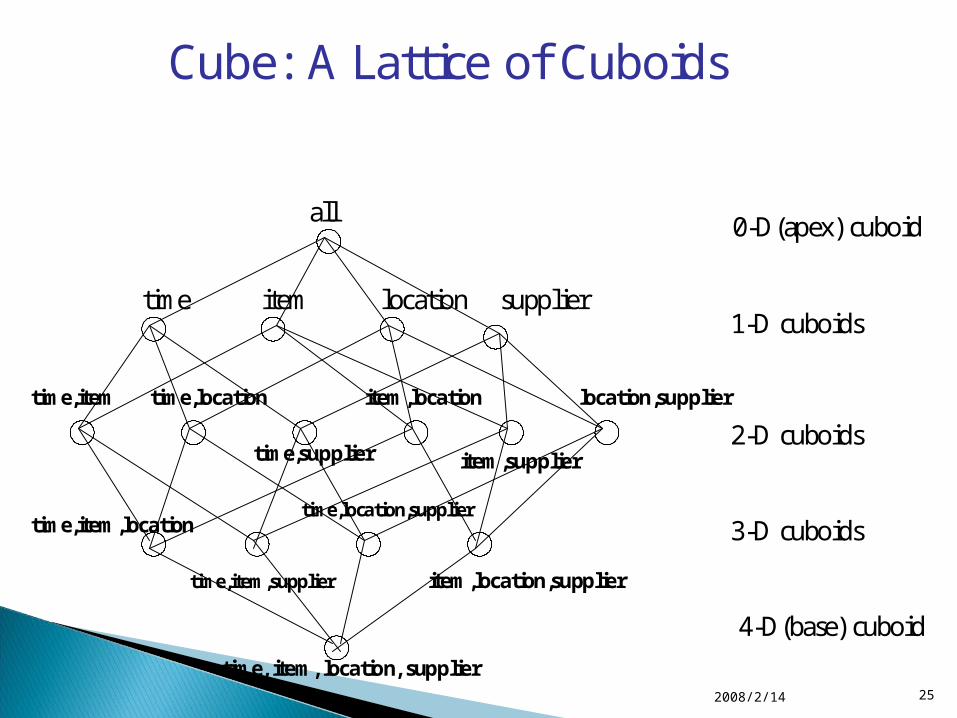
In data warehousing literature, an n-D base cube is called a base cuboid. The top most 0-D cuboid, which holds the highest-level of summarization, is called the apex cuboid. The lattice of cuboids forms a data cube.

2008/2/14 21

2008/2/14 22

OLTP OLAP

users clerk, IT professional knowledge worker

function day to day operations decision support

DB design application-oriented subject-oriented

data current, up-to-date detailed, flat relational isolated

historical, summarized, multidimensional integrated, consolidated

usage repetitive ad-hoc

access read/write index/hash on prim. key

lots of scans

unit of work short, simple transaction complex query

# records accessed tens millions

#users thousands hundreds

DB size 100MB-GB 100GB-TB

metric transaction throughput query throughput, response

Relational OLAP (ROLAP): ◦ Use relational or extended-relational DBMS to store and

manage warehouse data and OLAP middle ware to support missing pieces.

◦ Include optimization of DBMS backend, implementation of aggregation navigation logic, and additional tools and services

◦ greater scalability Multidimensional OLAP (MOLAP):

◦ Array-based multidimensional storage engine (sparse matrix techniques)

◦ fast indexing to pre-computed summarized data Hybrid OLAP (HOLAP):

◦ User flexibility, e.g., low level: relational, high-level: array. Specialized SQL servers:

◦ specialized support for SQL queries over star.snowflake schemas

2008/2/14 23

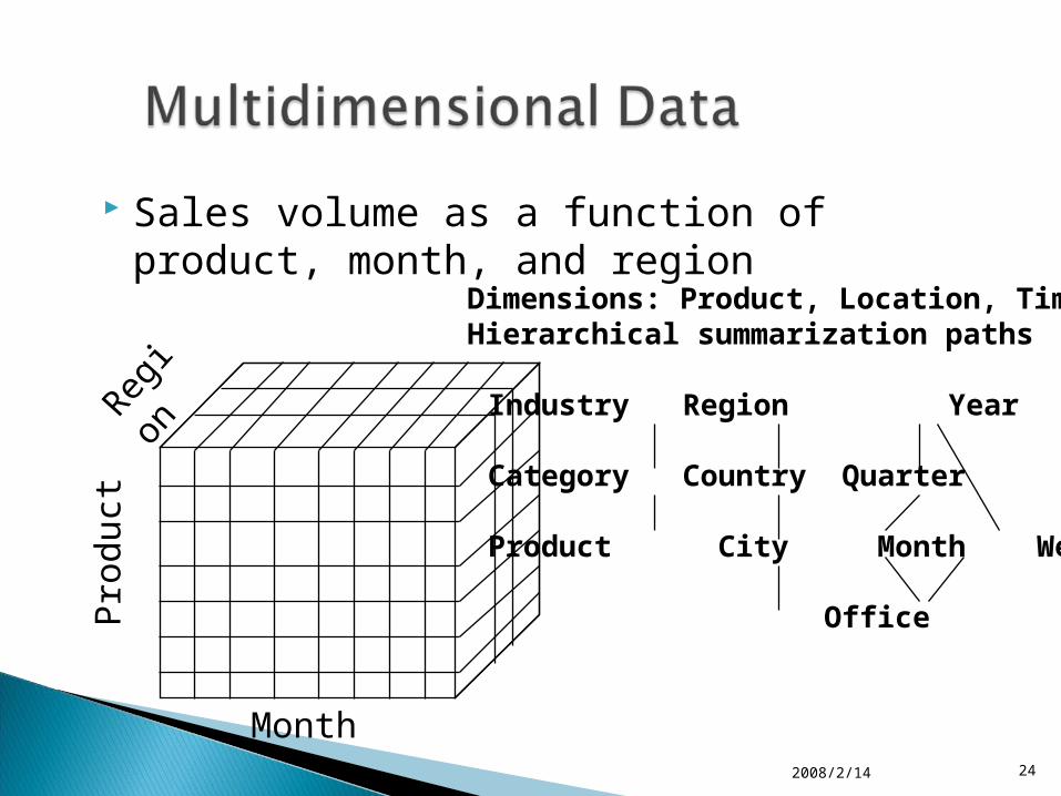
Sales volume as a function of product, month, and region

2008/2/14 24

Pro

duct

Regio

n

Month

Dimensions: Product, Location, TimeHierarchical summarization paths

Industry Region Year

Category Country Quarter

Product City Month Week

Office Day

2008/2/14 25

Cube: A Lattice of Cuboids

all

time item location supplier

time,item time,location

time,supplier

item,location

item,supplier

location,supplier

time,item,location

time,item,supplier

time,location,supplier

item,location,supplier

time, item, location, supplier

0-D(apex) cuboid

1-D cuboids

2-D cuboids

3-D cuboids

4-D(base) cuboid

Roll up (drill-up): summarize data◦ by climbing up hierarchy or by dimension reduction

Drill down (roll down): reverse of roll-up◦ from higher level summary to lower level summary or

detailed data, or introducing new dimensions Slice and dice:

◦ project and select Pivot (rotate):

◦ reorient the cube, visualization, 3D to series of 2D planes.

Other operations◦ drill through: through the bottom level of the cube to

its back-end relational tables (using SQL)2008/2/14 26

2008/2/14 27

2008/2/14 28

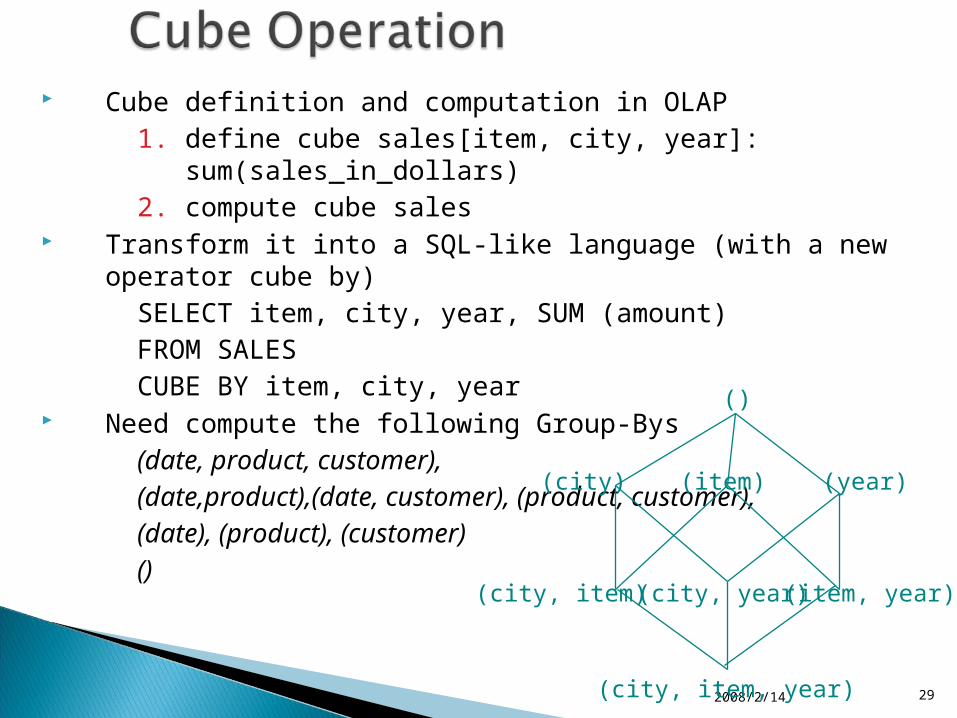
Cube definition and computation in OLAP1. define cube sales[item, city, year]: sum(sales_in_dollars)2. compute cube sales

Transform it into a SQL-like language (with a new operator cube by)

SELECT item, city, year, SUM (amount)FROM SALESCUBE BY item, city, year

Need compute the following Group-Bys (date, product, customer),(date,product),(date, customer), (product, customer),(date), (product), (customer)()

2008/2/14 29

(item)(city)

()

(year)

(city, item) (city, year) (item, year)

(city, item, year)

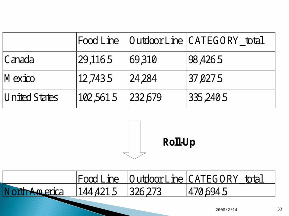
The roll-up operation performs aggregation on a data cube, either by climbing up a concept hierarchy for a dimension or by dimension reduction such that one or more dimensions are removed from the given cube.

Drill-down is the reverse of roll-up. It navigates from less detailed data to more detailed data. Drill-down can be realized by either stepping down a concept hierarchy for a dimension or introducing additional dimensions.

2008/2/14 30

The slice operation performs a selection on one dimension of the given cube, resulting in a sub_cube.

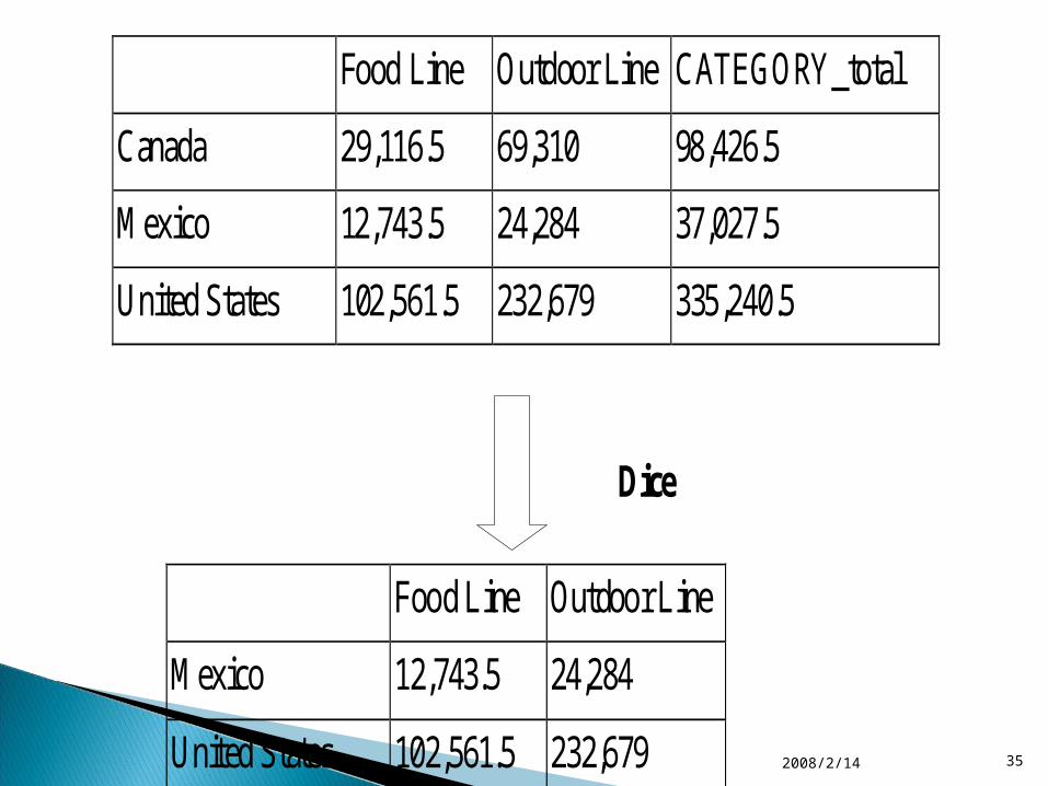
The dice operation defines a sub_cube by performing a selection on two or more dimensions.

2008/2/14 31

2008/2/14 32

Food Line Outdoor Line CATEGORY_total Asia 59,728 151,174 210,902

Food Line Outdoor Line CATEGORY_total

Malaysia 618 9,418 10,036

China 33,198.5 74,165 107,363.5

India 6,918 0 6,918

Japan 13,871.5 34,965 48,836.5

Singapore 5,122 32,626 37,748

Belgium 7797.5 21,125 28,922.5

Drill-Down

2008/2/14 33

Roll-Up

Food Line Outdoor Line CATEGORY_total

Canada 29,116.5 69,310 98,426.5

Mexico 12,743.5 24,284 37,027.5

United States 102,561.5 232,679 335,240.5

Food Line Outdoor Line CATEGORY_total North America 144,421.5 326,273 470,694.5

Slice

Food Line Outdoor Line CATEGORY_total North America 144,421.5 326,273 470,694.5

992,481690,751301,730REGION_total

470,694.5326,273144,421.5North America

310,884.5213,30497,580.5Europe

210,902151,17459,728Asia

CATEGORY_total

Outdoor Line

Food Line

992,481690,751301,730REGION_total

470,694.5326,273144,421.5North America

310,884.5213,30497,580.5Europe

210,902151,17459,728Asia

CATEGORY_total

Outdoor Line

Food Line

2008/2/14 34

2008/2/14 35

Food Line Outdoor Line

Mexico 12,743.5 24,284

United States 102,561.5 232,679

Dice

Food Line Outdoor Line CATEGORY_total

Canada 29,116.5 69,310 98,426.5

Mexico 12,743.5 24,284 37,027.5

United States 102,561.5 232,679 335,240.5

The select clause defines axis dimensions on COLUMNS and on ROWS, where clause supplies slicer dimensions, and Cube is the name of the data cube.

Select axis [, axis]From CubeWhere slicer [, slicer]

2008/2/14 36

For the majority of MDX statements, the context of the query will be limited to a single cube. It is important to know how all data within a cube is divided into the following relationship:

Dimensions Hierarchies Levels Members

2008/2/14 37

SELECT {[Gender].[Gender].Members} ON COLUMNS,{[Product].[Product Family].Members} ON ROWS,FROM [Sales]WHERE([Measures].[Unit Sales],[Customers].[All Customers],[Education Level].[All Education Level],[Marital Status].[All Martial status],[Promotions].[All Promotions],[Store].[All Stores],[Store Size in SQFT].[All],[Store Type].[All],[Yearly Income].[All Yearly Income]

2008/2/14 38

Example on Star Schema

2008/2/14 39

FT_sales

time_idstorecodedocnopluqtyamount

DM_store

storecodearealocationtypesize_rangesales_range

DM_product

pluseason_codecolor_codesize_code

DM_time

time_idthe_datethe_daythe_monththe_yearquarterweek_day1week_day2day_num

2008/2/19 40

SELECT [SALES].[AMOUNT] ON COLUMNS, SELECT [SALES].[AMOUNT] ON COLUMNS,

[store].[Kowloon][store].[Kowloon] ON ROWS ON ROWS

FROM SALESFROM SALES

MDX

SQLselect sum(amount), area select sum(amount), area from SALES from SALES where (area='Kowloon') group by areawhere (area='Kowloon') group by area

Graphical Description on Roll-up Example

2008/2/14 41

Tim

e

Store (store code)

100 200 ... ... 300 400

217 ... ... 268204 292

All

time

100 200 ... ...100 200 ... ...

100 200 ... ...100 200 ... ...

Tim

eStore (area)

NTHK

All

time

Kln.

1800 2500 3200

Roll-up on Store Dimension(from store to area)

Store is the child of Area

2008/2/19 42

SELECT [SALES].[AMOUNT] ON COLUMNS, SELECT [SALES].[AMOUNT] ON COLUMNS,

[time].[2003].[Q4].[Dec].[31],[time].[2003].[Q4].[Dec].[31],

[time].[2003].[Q4].[Dec].[30],… …, [time].[2003].[Q4].[Dec].[30],… …,

[time].[2003].[Q4].[Dec].[2], [time].[2003].[Q4].[Dec].[2],

[time].[2003].[Q4].[Dec].[1][time].[2003].[Q4].[Dec].[1] ON ROWS FROM SALES ON ROWS FROM SALES

MDX

SQLselect sum(amount), the_date select sum(amount), the_date from SALES from SALES where (the_date='2003-Dec-31')where (the_date='2003-Dec-31')or (the_date='2003-Dec-30')or (the_date='2003-Dec-30')or… …or (the_date='2003-Dec-2') or… …or (the_date='2003-Dec-2') or (the_date='2003-Dec-1') group by the_dateor (the_date='2003-Dec-1') group by the_date

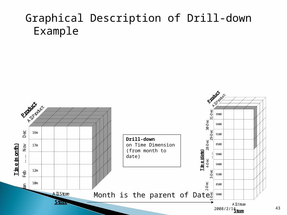
Graphical Description of Drill-down Example

2008/2/14 43

Tim

e (m

onth

)

Store

10m

12m

17m

16m

All Store

Jan

Dec

Nov

... ..

.Fe

b Tim

e (d

ate)

Store

All Store

All Pro

duct

1-D

ec31

-Dec

30-D

ec...

...

2-D

ec29

-Dec

28-D

ec4-

Dec

3-D

ec

9900

8500

9100

9400

9900

8500

9100

9400

9900

9900

8500

9100

9400

9900

8500

9100

9400

9900

9900

8500

9100

9400

9900

8500

9100

9400

9900

9900

8500

9100

9400

9900

8500

9100

9400

9900

Drill-down on Time Dimension(from month to date)

Month is the parent of Date

2008/2/19 44

MDX

SQL

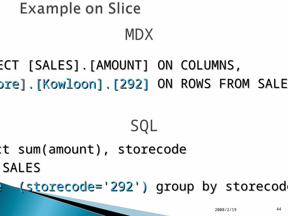
SELECT [SALES].[AMOUNT] ON COLUMNS, SELECT [SALES].[AMOUNT] ON COLUMNS,

[store].[Kowloon].[292][store].[Kowloon].[292] ON ROWS FROM SALES ON ROWS FROM SALES

select sum(amount), storecode select sum(amount), storecode

from SALES from SALES

where (storecode='292')where (storecode='292') group by storecode group by storecode

Graphical Description of Slice

2008/2/14 45

Tim

e

Store (store code)

100 200 ... ... 300 400

217 ... ... 268204 292

Product

All

tim

e

All Pro

duct

Slice WHERE store = ‘292’

Tim

eStore (store code)

400

292

All

tim

e

2008/2/19 46

MDX

SQL

SELECT [SALES].[AMOUNT] ON COLUMNS, SELECT [SALES].[AMOUNT] ON COLUMNS,

[store].[HK],[store].[NT], [store].[Kowloon] ON ROWS [store].[HK],[store].[NT], [store].[Kowloon] ON ROWS

FROM SALES FROM SALES WHERE [time].[2003].[Q4].[Dec].[24WHERE [time].[2003].[Q4].[Dec].[24]]

select sum(amount), area select sum(amount), area from SALES from SALES wherewhere ( (area='HK') or (area='NT') or (area='Kowloon')) ( (area='HK') or (area='NT') or (area='Kowloon'))andand (the_date='2003-Dec-24') (the_date='2003-Dec-24') group by areagroup by area

Graphical Description of Dice

2008/2/14 47

Tim

e (m

onth

)

Store

10m

12m

17m

16m

Product

All Pro

duct

Jan

Dec

Nov

... ..

.Fe

b

217 ... ... 292291244

16m16m

16m16m

Tim

e (m

onth

)

Store

14m

Dec

292

Dice WHERE (store = ‘292’) and (time = ‘Dec’) and product = ‘ALL’

The CrossJoin ( ) function is used to generate the cross-product of two input sets. If two sets exist in two independent dimensions, the CrossJoin operator creates a new set consisting of all of the combinations of the members in the two dimensions.

2008/2/14 48

In some respects, the Filter ( ) function and the slicer axis have similar purposes. The difference between the two is that the Filter ( ) function defines the members in a set, while slicers determine a slice of the cube returned from a query.

2008/2/14 49

The Order ( ) function provides sorting capabilities within the MDX language. When the Order expression is used, it can either sort within the natural hierarchy (ASC and BDESC), or it can sort without the hierarchy (BASC and BDESC). The “B” indicates “break” hierachy.

2008/2/14 50

The TopCount () and BottomCount() functions provide rank functionality critical in a decision support and data analysis environment. These expressions sort a set based on a numerical expression and pick the top index items based on rank order.

2008/2/14 51

Gender_member

Product name

All_Marital_status

Gender dimension tableMarital_status dimension table

Product dimension table

Measure fact table

Gender_member

Product_name

All_Marital_status

Promotions

Store

Yearly Income

Unit_SalesStore CostStore SalesSales Count,Store Sales Net

Promotions

StoreYearly income

Store dimension table

Promotion dimension table

Yearly dimension table

Year

Year

Time dimension table

2008/2/17 52

Dimension tables:[Gender].[Gender Members][Product].[Product Name][Marital Status].[All Martial status][Promotions].[All Promotions],[Store].[All Stores],[Store Size in SQFT].[All],[Store Type].[All],[Yearly Income].[All Yearly Income][Time].[Year]

Fact table:[Measures].[Unit Sales],[Measures].[Store Cost],[Measures].[Store Sales],[Measures].[Sales Count],[Measures].[Store Sales Net]

2008/2/14 53

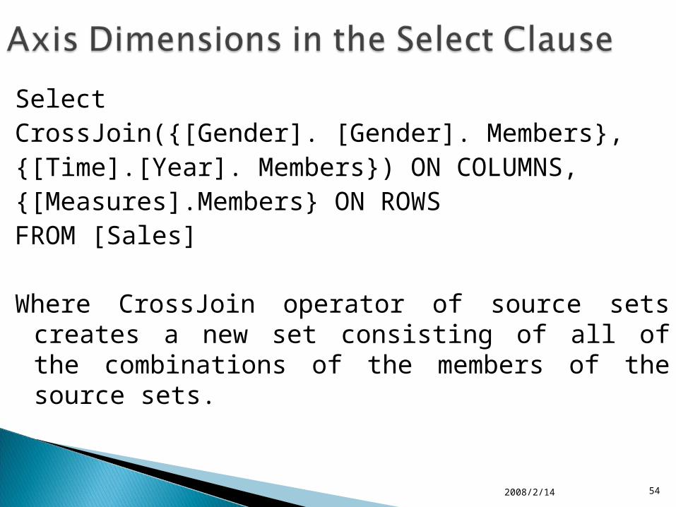
SelectCrossJoin({[Gender]. [Gender]. Members},{[Time].[Year]. Members}) ON COLUMNS,{[Measures].Members} ON ROWSFROM [Sales]

Where CrossJoin operator of source sets creates a new set consisting of all of the combinations of the members of the source sets.

2008/2/14 54

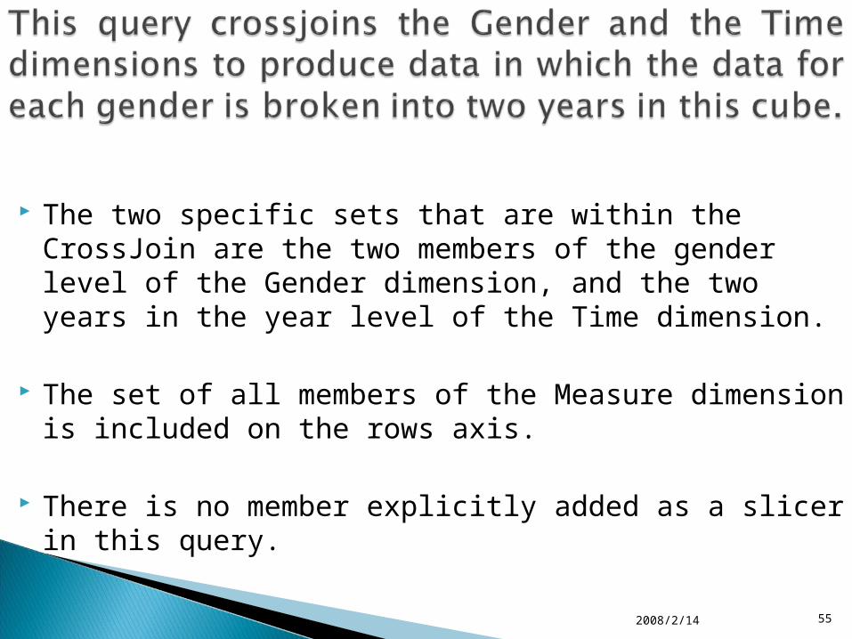
The two specific sets that are within the CrossJoin are the two members of the gender level of the Gender dimension, and the two years in the year level of the Time dimension.

The set of all members of the Measure dimension is included on the rows axis.

There is no member explicitly added as a slicer in this query.

2008/2/14 55

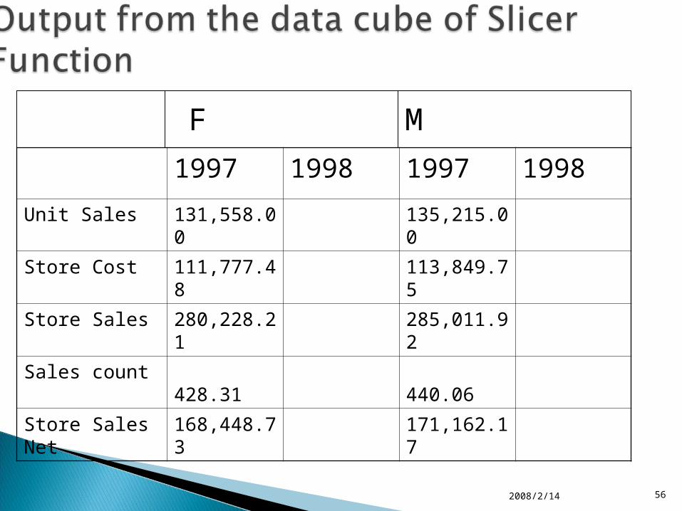
1997 1998 1997 1998

Unit Sales 131,558.00 135,215.00

Store Cost 111,777.48 113,849.75

Store Sales 280,228.21 285,011.92

Sales count 428.31 440.06

Store Sales Net 168,448.73 171,162.17

2008/2/14 56

F M

SELECT{[Measures]. [Unit Sales]} ON COLUMNS,{Filter({[Product]. [Product

Department].Members},([Gender]. [All Gender].[F],[Measures].[Unit Sales])

> 10000)} ON ROWSFROM [Sales]

2008/2/14 57

The results of this query show that the set returned on the rows axis consists of product departments for which unit sales to females is greater than $10000

2008/2/17 58

Unit Sales

Frozen Food 26,655.00

Produce 37,792.00

Snack Foods 30,545.00

Household 27,038.00

2008/2/14 59

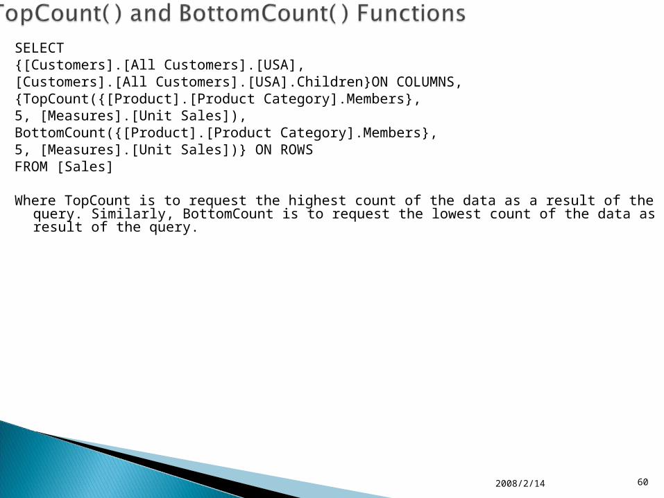
SELECT {[Customers].[All Customers].[USA],[Customers].[All Customers].[USA].Children}ON COLUMNS,{TopCount({[Product].[Product Category].Members},5, [Measures].[Unit Sales]),BottomCount({[Product].[Product Category].Members},5, [Measures].[Unit Sales])} ON ROWSFROM [Sales]

Where TopCount is to request the highest count of the data as a result of the query. Similarly, BottomCount is to request the lowest count of the data as a result of the query.

2008/2/14 60

The product categories are included on the rows axis in a comma-separated list where different operators are used to specify a particular subset of the [Product].[Product Category]. Members set. Unit sales is used as the measure with which to select the top five product categories and the bottom five product categories.

2008/2/14 61

USA CA OR WASnack Foods 30,545.00 8,543.00 7,789.00 14,213.00Vegetables 20,733.00 5,506.00 5,447.00 9,306.00Dairy 12,885.00 3,534.00 3,131.00 6,220.00Jams & Jelies 11,888.00 3,343.00 2,877.00 5,868.00Fruit 11,767.00 3,184.00 3,008.00 5,575.00Canned Oysters 708.00 220.00 182.00 296.00Canned Shimp 804.00 231.00 173.00 400.00Hardware 810.00 281.00 215.00 334.00Candies 815.00 286.00 248.00 303.00Canned Food 819.00 234.00 215.00 370.00

2008/2/14 62

Select{[Marital Status].[All Marital Status].[S]} ON

COLUMNS,{Order ({[Promotion Media].[Media Type].Members},[Unit Sales], BDESC)} ON ROWSFROM [Sales]

Where BDESC means sort descending without hierarchy.

2008/2/14 63

The sort was performed using the [Marital Status] .[All Marital Status].[S] member in descending order without hierarchy of the unit sales.

2008/2/17 64

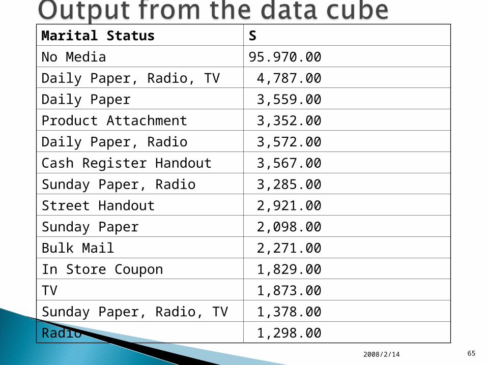
Marital Status S

No Media 95.970.00

Daily Paper, Radio, TV 4,787.00

Daily Paper 3,559.00

Product Attachment 3,352.00

Daily Paper, Radio 3,572.00

Cash Register Handout 3,567.00

Sunday Paper, Radio 3,285.00

Street Handout 2,921.00

Sunday Paper 2,098.00

Bulk Mail 2,271.00

In Store Coupon 1,829.00

TV 1,873.00

Sunday Paper, Radio, TV 1,378.00

Radio 1,298.00

2008/2/14 65

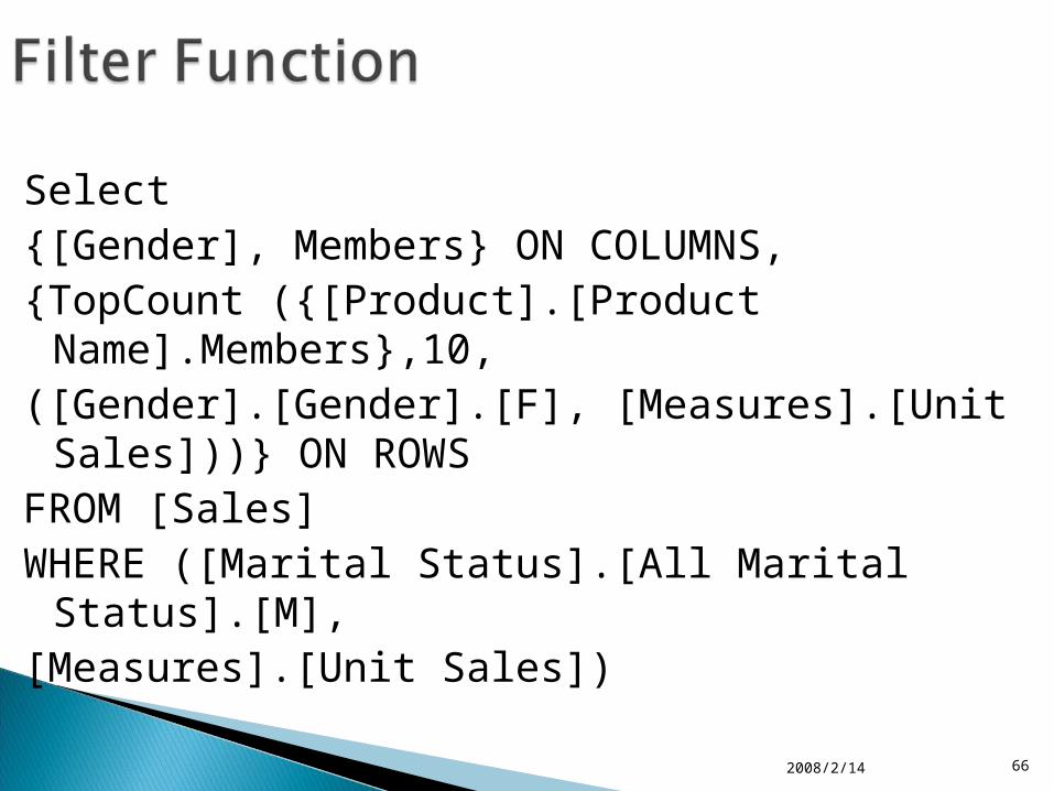
Select{[Gender], Members} ON COLUMNS,{TopCount ({[Product].[Product

Name].Members},10, ([Gender].[Gender].[F], [Measures].[Unit Sales]))}

ON ROWSFROM [Sales]WHERE ([Marital Status].[All Marital Status].[M],[Measures].[Unit Sales])

2008/2/14 66

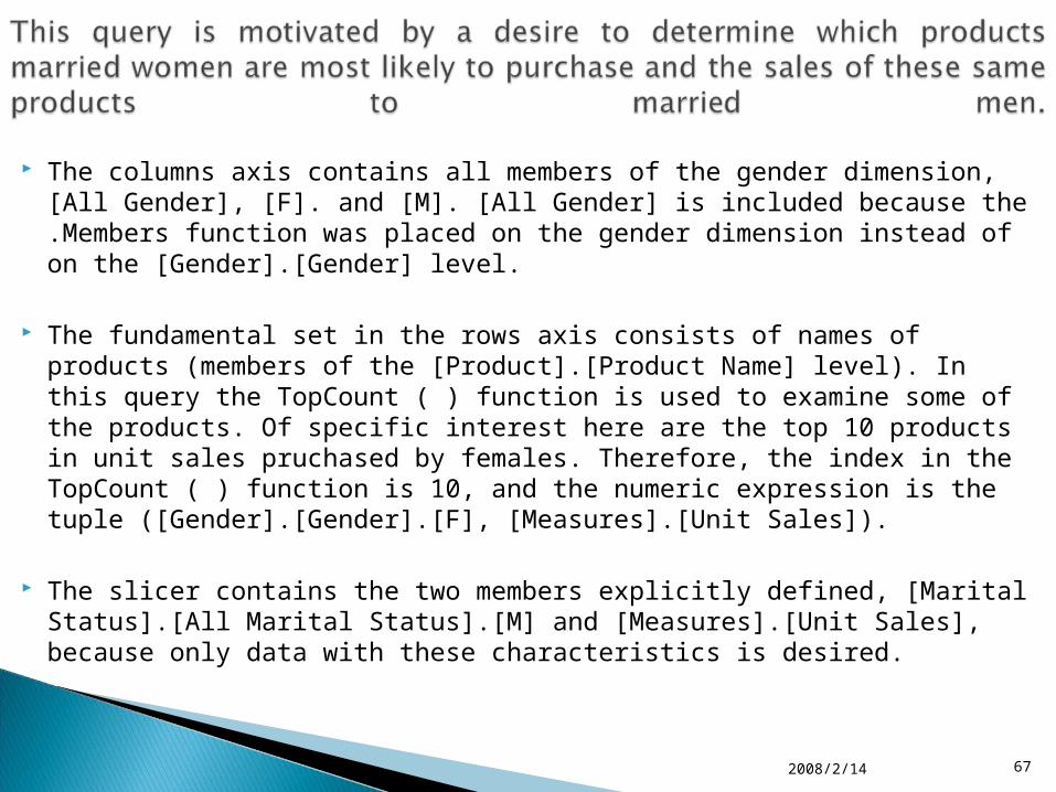
The columns axis contains all members of the gender dimension, [All Gender], [F]. and [M]. [All Gender] is included because the .Members function was placed on the gender dimension instead of on the [Gender].[Gender] level.

The fundamental set in the rows axis consists of names of products (members of the [Product].[Product Name] level). In this query the TopCount ( ) function is used to examine some of the products. Of specific interest here are the top 10 products in unit sales pruchased by females. Therefore, the index in the TopCount ( ) function is 10, and the numeric expression is the tuple ([Gender].[Gender].[F], [Measures].[Unit Sales]).

The slicer contains the two members explicitly defined, [Marital Status].[All Marital Status].[M] and [Measures].[Unit Sales], because only data with these characteristics is desired.

2008/2/14 67

All Gender F MFabulous Berry Juice 127.00 87.00 40.00Fast Beef Jerky 134.00 87.00 47.00BBB Best Pepper 134.00 82.00 52.00Ebony Cantelope 130.00 80.00 50.00Peart Cheable Wine 117.00 79.00 38.00Skinner Diel Cola 115.00 78.00 37.00Shdy Lake Manicotti 106.00 78.00 28.00Pearl Light Beer 130.00 77.00 53.00Shady Lake Rice Medly 131.00 77.00 54.00TriState Potatos 108.00 76.00 32.00

2008/2/14 68

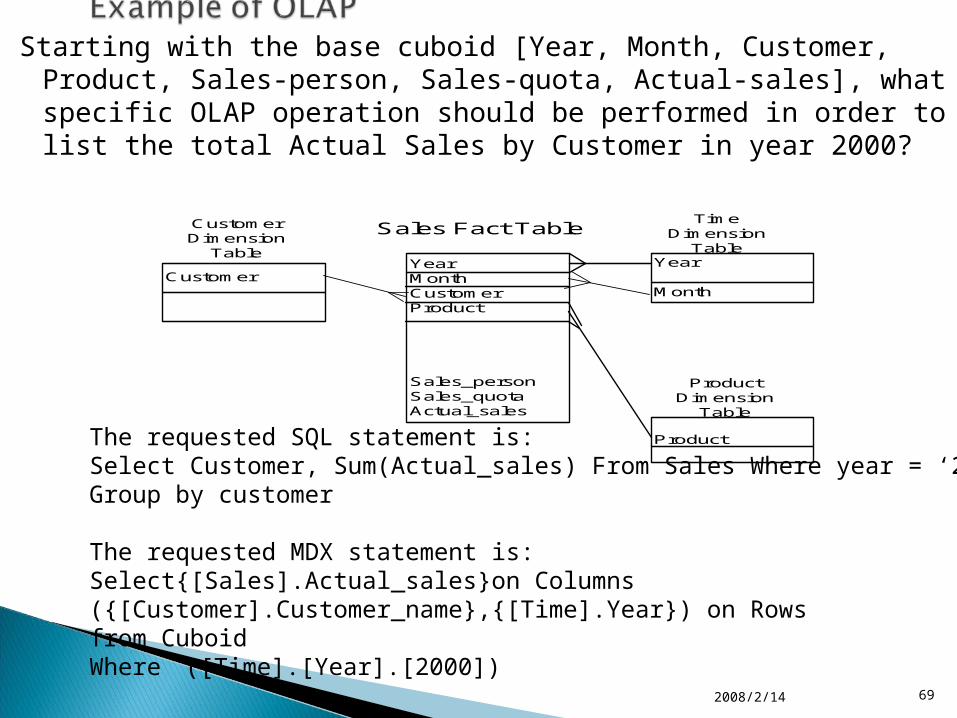
Starting with the base cuboid [Year, Month, Customer, Product, Sales-person, Sales-quota, Actual-sales], what specific OLAP operation should be performed in order to list the total Actual Sales by Customer in year 2000?

2008/2/14 69

CustomerYearMonthCustomerProduct

Sales_personSales_quotaActual_sales

Year

Month

Product

TimeDimension

Table

Sales Fact TableCustomerDimension

Table

ProductDimension

Table

The requested SQL statement is:Select Customer, Sum(Actual_sales) From Sales Where year = ‘2000’ Group by customer

The requested MDX statement is:Select{[Sales].Actual_sales}on Columns({[Customer].Customer_name},{[Time].Year}) on Rowsfrom CuboidWhere ([Time].[Year].[2000])

“Data Mining: Concepts and Techniques” Second edition by Han and Kamber, Morgan Kaufmann publishers, 2007, chapter 3, pp. 123-154.

2008/2/14 70

Discuss three methods of implementing an online analytical processing command. Give an example of using one of them with a given Star schema.

2008/2/14 71

Suppose that a data warehouse consists of the three dimensions time, doctor, and patent, and the two measures count and charge, where charge is the fee that a doctor charges a patient for a visit. Starting with the base cuboid [day, doctor, patient], provide a MDX (Multidimensional Expression) query to list the total fee collected by each doctor in 2000?

To obtain the same list, write an SQL query assuming the data is stored in a relational database with the table fee (day, month, year, doctor, hospital, patient, count, charge).

1. Starting with the base cuboid [day, doctor, patient], provide a MDX (Multidimensional Expression) query to list the total fee collected by each doctor in 2000?

2. To obtain the same list, write an SQL query assuming the data is stored in a relational database with the table fee (day, month, year, doctor, hospital, patient, count, charge).

2008/2/14 72

Doctor_id

Hospitaldoctor_namephone#addresssex

time_keydoctor_idpatient_id

chargecount

Time_key

dayday_of_weekmonthquarteryear

Patient_id

patient_namephone#sexdescriptionaddress

Time dimension tableFee fact tableDoctor dimension table

Patient dimension table