˘ ˇˆ - productivity commission preferential trading arrangement or agreement roo rules of origin...
TRANSCRIPT
����������������� ����������������������������������
������� �������������������������
������������������
�� �!""#
�������������� ����������������� �������������
����������$���������������������������������������������������������������������� �������������������������%����� &� ������'����������������������������������������'
Inquiries about this staff working paper:
Media and PublicationsProductivity CommissionLocked Bag 2 Collins St EastMelbourne VIC 8003
Tel: (03) 9653 2244Fax: (03) 9653 2303Email: [email protected]
General Inquiries:
Tel: (03) 9653 2100 or(02) 6240 3200
Citation, with permission from the author(s), should read:
Adams, R., Dee, P., Gali, J. and McGuire, G. 2003, The Trade and Investment Effectsof Preferential Trading Arrangements — Old and New Evidence, ProductivityCommission Staff Working Paper, Canberra, May.
Information on the Productivity Commission, its publications and its current work program can befound on the World Wide Web at http://www.pc.gov.au or by contacting Media and Publications on(03) 9653 2244.
CONTENTS III
Contents
Acknowledgments VI
Abbreviations VII
Summary IX
1 Introduction 1
1.1 First wave 2
1.2 Second wave 3
1.3 Third wave 6
1.4 Outline of this paper 7
2 A review of the theory of PTAs 11
2.1 The static welfare effects of PTAs 11
2.2 The dynamic effects of PTAs on multilateral liberalisation 20
2.3 The effects of non-trade provisions of PTAs 23
2.4 Summary 27
3 Review of the existing empirical evidence 29
3.1 Approaches to assessing PTAs 29
3.2 Evidence on trade creation and diversion effects of PTAs —assessment of first wave issues 38
3.3 Evidence on stumbling or building blocks — assessment ofsecond wave issues 57
3.4 Evidence on investment creation and diversion effects of PTAs— assessment of third wave issues 59
3.5 Summary 61
4 New evidence on trade creation and diversion 63
4.1 Analytical issues 64
4.2 Model specification 72
4.3 Main results 76
4.4 Puzzles on new evidence 81

IV CONTENTS
4.5 Summary 84
5 Investment creation and diversion 87
5.1 ‘New age’ or third wave provisions in PTAs 87
5.2 Model specification and estimation 90
5.3 Impact of merchandise trade and ‘new age’ provisions oninvestment 94
5.4 Summary 97
6 Summing up 99
6.1 Trade provisions 99
6.2 Non-trade provisions 100
A Member Liberalisation Index 103
B Data sources 119
C Econometric estimation and issues 125
D Econometric results 131
References 139
BOXES
Box 1.1 GATT provisions governing PTAs 5
FIGURES
Figure 1.1 Member Liberalisation Index for selected PTAs 2
Figure 2.1 An illustration of trade creation and diversion effects of a PTA 12
Figure 3.1 Use of PTA-specific dummy variables in a gravity model — theexample of NAFTA 33
Figure A.1 Member Liberalisation Index for selected PTAs 106
Figure A.2 Merchandise and non-merchandise MLIs for selected PTAs 107
TABLES
Table 3.1 Normal bilateral trade determinants included in past gravitymodel studies 34
CONTENTS V
Table 3.2 Past estimates of trade creation and diversion effects of AndeanPact/Community 40
Table 3.3 Past estimates of trade creation and diversion effects ofLAFTA/LAIA 43
Table 3.4 Past estimates of trade creation and diversion effects ofMERCOSUR 44
Table 3.5 Past estimates of trade creation and diversion effects of NAFTA 47
Table 3.6 Past estimates of trade creation and diversion effects of CER 49
Table 3.7 Past estimates of trade creation and diversion effects ofASEAN-FTA 50
Table 3.8 Past estimates of trade creation and diversion effects of EC/EU 52
Table 3.9 Past estimates of trade creation and diversion effects of EFTA 56
Table 3.10 Building blocks or stumbling blocks to free trade 58
Table 4.1 Provisions covering agriculture and industrial products and theirweights in the merchandise MLI 66
Table 4.2 Membership dynamics in major PTAs 69
Table 4.3 New evidence on PTAs as causing net trade creation ordiversion 78
Table 5.1 Non-merchandise trade provisions and their weights in the MLI 88
Table 5.2 Main drivers of investment in PTAs 94
Table 5.3 New evidence on investment creation and diversion 95
Table 5.4 Net impact of PTAs’ third wave provisions on investment 96
Table A.1 Member Liberalisation Index 108
Table A.2 Member Liberalisation Index — detailed results 114
Table B.1 Full sample of countires in the gravity model 120
Table B.2 Summary statistics for selected PTAs, 1997 121
Table C.1 Marginal effects and Tobit estimates 128
Table D.1 Gravity model of trade — econometric results from full sample 131
Table D.2 Gravity model of trade — results from limited sample with tariffvariable included 134
Table D.3 Tests of significance of groups of PTA dummy coefficients forbilateral versus plurilateral agreements 136
Table D.4 Gravity model of investment 137
VI ACKNOWLEDGMENTS
Acknowledgments
The authors thank, without implication, all those who have commented on thepaper. David Robertson from the Productivity Commission, Richard Pomfret fromthe University of Adelaide and Peter Lloyd from the University of Melbourneprovided referees’ comments. Mark Harris, then at the University of Melbourne,provided detailed comments and advice on econometric issues. An earlier version ofpart of the paper was presented at the Australian Conference of Economists,Adelaide, 30 September to 3 October 2002.
ABBREVIATIONS VII
Abbreviations
Abbreviations
ABS Australian Bureau of Statistics
AFTA ASEAN Free Trade Area
ANZCERTA Australia New Zealand Closer Economic Relations TradeAgreement
APEC Asia Pacific Economic Cooperation
ASEAN Association of South East Asian Nations
BIT Bilateral Investment Treaty
CAP Common Agricultural Policy
CER Closer Economic Relations (short for ANZCERTA)
CGE Computable General Equilibrium models
CRTA Committee on Regional Trade Agreements
CUSFTA Canada United States Free Trade Area
EEC European Economic Community
EFTA European Free Trade Area
EU European Union
FDI Foreign Direct Investment
GATS General Agreement on Trade in Services
GATT General Agreement on Tariffs and Trade
GCC Gulf Cooperative Council
GDP Gross Domestic Product
GSP Generalised System of Preferences
IMF International Monetary Fund
LAFTA Latin American Free Trade Area
LAIA Latin American Integration Association
VIII ABBREVIATIONS
MERCOSUR Southern Common Market (Mercado Común del Cono Sur)
MFN Most Favoured Nation
MITI Ministry of International Trade and Industry
MLI Member Liberalisation Index
NAFTA North American Free Trade Agreement
OAS Organization of American States
OECD Organisation for Economic Cooperation and Development
PATCRA Papua New Guinea Agreement on Trade and CommercialRelations
PPP Purchasing power parity
PTA Preferential Trading Arrangement or Agreement
ROO Rules of Origin
RTA Regional Trading Arrangement or Agreement
SITC Standard International Trade Classification
SPARTECA South Pacific Regional Trade and Economic CooperationAgreement
SPS Sanity and Phytosanitary
UN United Nations
UNCTAD United Nations Conference on Trade and Development
WDI World Development Indicators
WTA World Trade Analyzer
WTF World Trade Flows database
WTO World Trade Organisation
SUMMARY

X SUMMARY
SUMMARY XI
Summary
The number of preferential trading arrangements (PTAs) has grown dramaticallyover the last decade or so. By the end of 2000, there were 191 agreements in forcethat had been notified to the World Trade Organisation, compared with 40 in 1990.
The coverage of preferential trading arrangements has also tended to expand overtime. The preferential liberalisation of tariffs and other measures governingmerchandise trade remains important in many agreements. But they increasinglycover a range of other issues — services, investment, competition policy,government procurement, e-commerce, labour and environmental standards.
This paper examines, both theoretically and empirically, the effects of the trade andnon-trade provisions of PTAs on the trade and foreign direct investment flows ofmember and non-member countries.
Trade provisions
Theoretical work has always highlighted that while the merchandise tradeprovisions of PTAs can boost trade among members, this is often at the expense ofnon-members. So whether it benefits a country to join a PTA depends on the coststructures in partner countries, compared with the cost structures in third parties. If apreferential trade arrangement diverts a country’s imports from a low-cost thirdparty to a higher-cost preferential trade partner, it can be made worse off.Conversely, the opportunity for benefits is greater where the PTA partner is atworld’s best competitiveness, and where liberalisation under the PTA encouragesimports from that source.
Traditionally, there have been two ways of evaluating the effects of PTAsempirically.
• Ex post econometric approaches. These cannot measure the effects of PTAs onthe economic welfare of member or non-member countries directly, since this isunobservable. But they can examine the effects of actual PTAs as written,complete with non-trade provisions, on actual trade and investment flows.
• Ex ante computable general equilibrium analyses. These generally have enougheconomic structure to be able to draw inferences about the economic welfare of
XII SUMMARY
member and non-member countries. But they typically have a very idealised andtariff-oriented treatment of PTA provisions.
Since the purpose of this paper is to shed light on the effects of the non-tradeprovisions of PTAs, it uses econometric techniques to look at the effects of someexisting PTAs, particularly those containing significant non-trade provisions, on theactual trade and investment flows of member and non-member countries.
Because the paper uses econometric techniques, it cannot look at PTAs in prospect(including those being negotiated by Australia). And while it can examine theeffects of existing PTAs on trade and investment flows, it cannot draw strong directinferences about the consequences for economic welfare. The trade and investmenteffects are not always good indicators of the likely welfare effects, as elaborated inthe next chapter. But trade and investment effects are still likely to be of interest intheir own right.
New empirical work outlined in chapter 4 suggests that of the 18 recent PTAsexamined in detail, 12 have diverted more trade from non-members than they havecreated among members. What is more, some of the apparently quite liberal PTAs— including EU, NAFTA and MERCOSUR — have failed to create significantadditional trade among members (relative to the average trade changes registeredamong countries in the sample).
Part of the reason for this more negative finding than in previous studies is therigorous statistical test that has been applied to ascertain whether intra-bloc trade issignificantly greater after bloc formation (or expansion) than before. In the past, thiswas assessed, at best, only by reference to the point estimates from various crosssections. But the finding is also consistent with the observation that many of theprovisions needed in preferential arrangements to underpin and enforce theirpreferential nature — such as rules of origin — are in practice quite traderestricting.
Non-trade provisions
While the increasing focus of PTAs on non-trade provisions may suggest thatconventional concerns about trade diversion are outmoded, some theoreticalliterature suggests that such a conclusion would be premature.
On the one hand, in an increasingly integrated world economy, even minor tradeconcessions can have a significant impact on investment flows. And if investment isattracted into one PTA partner in order to serve the markets of the others, then thetrade from such ‘beachhead’ positions can constitute traditional trade diversion.
SUMMARY XIII
On the other hand, the non-trade provisions of PTAs, particularly those related toinvestment and services, can also have a significant impact on investment flows. Butthe preferential nature of the PTA provisions may mean that investment is divertedfrom a low-cost to a higher-cost host country, and such investment diversion canalso be harmful.
The analysis in chapter 5 is among the first to check these propositions empirically.It finds little evidence of beachhead investment, or an unwinding of ‘tariff-jumping’investment, in response to the trade provisions of PTAs. Only for SPARTECA andthe US-Israel agreement, for example, is there (weak) evidence of foreign directinvestment responding in beachhead fashion to trade provisions. And the result forUS-Israel is further qualified by the imprecision of the intra-bloc effect with justtwo countries involved.
Chapter 5 does find evidence that foreign direct investment responds significantly tothe non-trade provisions of PTAs. Interestingly, this is in contrast to a lack ofresponse of FDI to bilateral investment treaties.
Further, for most of those agreements where non-trade provisions have affectedFDI, the result has been net investment creation rather than diversion.
Although it is a weak test, this suggests that on balance, the non-trade provisions ofthese PTAs have created an efficient geographic distribution of FDI. This isconsistent with the fact that at least some of the non-trade provisions (egcommitments to more strongly enforce intellectual property rights ) are not stronglypreferential in their nature.
Further, the theoretical literature has stressed that if the non-trade barriers are of thesort to raise the real resource costs of doing business, rather than simply to createrents that raise prices above costs, then preferential liberalisation will be beneficial,even in the absence of net investment creation.
However, the trade that may be generated from the new FDI positions may still bediverted in the ‘wrong’ direction in response to the trade provisions of PTAs, andmay therefore contribute to the net trade diversion found in chapter 4.
Thus the results of this research suggest that there may be real economic gains fromthe non-trade provisions of third-wave PTAs, but they also suggest that there arestill economic costs associated with the preferential nature of the trade provisions.And these costs could be magnified in a world of increasing capital mobility.
Thus the findings of this research on the effects of the non-trade provisions of PTAsare more positive than those on the trade provisions. This suggests there could bereal benefits if countries could use regional negotiations to persuade trading partners

XIV SUMMARY
to make progress in reforming such things as investment, services, competitionpolicy and government procurement, especially if this is done on a non-preferentialbasis.

INTRODUCTION 1
1 Introduction
On 13 January 2002, the Prime Ministers of Japan and Singapore signed anagreement to create a preferential trading arrangement. The event is noteworthy, notjust because the bilateral arrangement is between two of Australia’s major tradingpartners. Until then, Japan had been the last major economy in the world not tobelong to a preferential trading arrangement.1
The agreement itself typifies many of the so-called ‘third wave’ of preferentialtrading arrangements, or PTAs.
In third wave agreements, provisions governing merchandise trade are often lessimportant than they were in the first or second waves, at least in relative terms. Inthe case of Japan and Singapore, both countries already have zero or very low tariffson imports of non-agricultural products. Trade in agricultural products betweenthem is minimal, but because of the sensitivity of the trade in cut flowers andgoldfish, agricultural and fishery products (along with some petrochemical andpetroleum goods) have been excluded from the bilateral agreement altogether.
Third wave agreements cover an increasing range of ‘new age’ issues — these caninclude services, investment, competition policy, government procurement, e-commerce, labour and environmental standards. In the Japan-Singapore EconomicAgreement for a New Age Partnership, as it is called, e-commerce and services areof particular importance.
Figure 1.1 shows the discernible upward trend in the breadth of coverage of PTAsover recent times. On the vertical axis is an index measure of breadth of coverage,with provisions governing merchandise and non-merchandise trade scoredseparately. The index is described in appendix A and has been applied to a numberof separate PTAs that have been established or had their membership changed inrecent times. On the horizontal axis is date of establishment. Coverage has clearlytended to increase in the more recently established or expanded PTAs, and this hasgenerally been because of an expansion in the coverage of non-merchandise tradeissues.
1 APEC (to which Japan belongs) is not a preferential arrangement. The Bogor goals of free and
open trade and investment by 2010 (for developed economies) and 2020 (for developingeconomies) are intended to be achieved on a non-discriminatory, most favoured nation basis.

2 TRADE ANDINVESTMENTEFFECTS OF PTAS
Figure 1.1 Member Liberalisation Index for selected PTAsIndex score ranges between zero and one
0.00.10.20.30.40.50.60.70.8
EU
(19
58)
EF
TA
(19
60)
AN
DE
AN
(19
69)
EU
-Sw
itz (
1973
)
PA
TC
RA
(19
77)
EU
-Egy
pt (
1978
)
LAIA
(19
80)
SP
AR
TE
CA
(19
81)
AN
ZC
ER
TA
(19
83)
Isra
el-U
S (
1985
)
AS
EA
N-F
TA
(19
92)
ME
RC
OS
UR
(19
91)
Chi
le-C
olom
bia
(199
3)
NA
FT
A (
1989
/199
3)
EU
-Pol
and
(199
4)
Chi
le-M
ER
CO
SU
R (
1996
)
Chi
le-M
exic
o (1
999)
Sin
gapo
re-N
Z (
2000
)
PTA (and its date of establishment)
Sco
re
Merchandise trade Non-merchandise trade
Data source: Appendix A.
1.1 First wave
By contrast, the ‘first wave’ of PTAs was more limited in scope, and preferentialliberalisation of merchandise trade generally played a more central role (EU beingan important early exception). In part, this was because general tariff levels werehigher to start with.
A key event in the first wave was the formation of the European EconomicCommunity (now European Union) in 1958, after several political agreements failedat the draft stage. Although EEC establishment was driven primarily by the politicalgoal of cementing European unity after two disastrous World Wars, internal tradeliberalisation was an important economic feature.
There was also a number of attempts to create PTAs among developing countries.These were aimed at reducing the costs of import-substituting industrialisation bypreferentially opening up the markets of the developing country members andexploiting economies of scale within that forum.
The focus of theoretical work on PTAs at the time was to challenge the popularnotion that any sort of trade liberalisation, even preferential, was a step in the right
INTRODUCTION 3
direction, and therefore beneficial to PTA members and to the world as a whole.The static analysis of PTAs, begun by Viner (1950), pointed out that although PTAformation reduced one distortion, namely, the average tariff on imports in general, itexacerbated another, namely, the geographical disparity in import tariffs. This was aclassic situation of ‘second best’, with no clear presumption in favour of gains toeither members or the world as a whole. The final outcome has defiedgeneralisation, though many analysts have chanced their arm. The answer‘depends’, and the devil is in the detail. The static theory of gains and losses frompreferential trading arrangements is summarised in chapter 2.
The literature has also recognised that if the answer ‘depends’, then the question isan empirical one. Various analysts have examined the trade effects of various PTAs,trying to determine whether they have encouraged imports in general — tradecreation — more than they have pushed the geographic source of imports in the‘wrong’ (higher cost) direction — trade diversion. There is a degree of apparentconsensus about which PTAs have been beneficial and which have not. There havealso been recent generalisations that PTAs as a whole are generally beneficial. Theexisting empirical literature on trade creation and trade diversion is reviewed inchapter 3.
1.2 Second wave
By the end of the 1960s, the PTAs established among developing countries as partof the first wave had largely collapsed.
The problem was that, rather than use trade liberalisation and hence prices to guideindustry allocation, the developing countries attempting such unions sought to allocateindustries by bureaucratic negotiation and to tie trade to such allocations, putting thecart before the horse and killing the forward motion. (Bhagwati 1999, p. 10)
The European Union (and its use of PTAs as a foreign policy instrument) is themain legacy from the first wave.
Interest in PTAs revived early in the 1980s as the United States reacted first to EUexpansionism and the loss of EU markets, and then to the uncertain prospects forlaunching the Uruguay Round, by selecting partners for bilateral and regional tradearrangements.
The United States had emerged from the 1930s experience of competitive tariffprotection with a strong distaste for preferential trading arrangements and a firmcommitment to multilateral trade liberalisation and the most favoured nation (MFN)principle — that trade concessions granted to any individual member of what wasthen the General Agreement on Tariffs and Trade (GATT) must be extended to all
4 TRADE ANDINVESTMENTEFFECTS OF PTAS
other GATT members. This was in contrast to the British, who wanted acontinuation of the Imperial Preferences in their favour. Although the US positiondid not rule out discrimination against non-GATT-members, it ensured tradeconcessions must be extended to countries accounting for the overwhelming bulk ofworld trade in any given commodity. The United States acceded to Article XXIV ofthe GATT, which allowed the formation of preferential trading arrangements undercertain circumstances. Box 1.1 gives a brief description of the provisions of ArticleXXIV, along with the two other mechanisms by which PTAs can be created in aGATT-consistent fashion. The United States also supported the formation of theEuropean Community for strategic political reasons. But prior to the 1980s, it hadnot entered any preferential trading arrangements of its own. Thus its entry intopreferential arrangements, first with Israel, then with Canada (through CUSTFA),Mexico (through NAFTA), and Caribbean countries (through the Caribbean BasinInitiative) represented a significant change in position.
The second wave of PTAs saw the inclusion of non-tariff barriers and other non-traditional areas, such as dispute resolution and competition policy. However, thesectoral focus remained on goods markets.
Rules of origin also became important. This was because the second waveagreements were predominantly free trade agreements, where members retainedtheir own external tariffs against non-members, in contrast to the EEC, which as acustoms union adopted a common external tariff. In free trade areas, rules of originwere needed, because otherwise there would be ‘trade deflection’ — imports wouldenter through the country with the lowest external tariff and then be re-exportedduty-free to other members. For example, one common type of rule specified that aproduct must have a given portion of its value added originating in the PTA beforeit qualified for duty-free movement to other member countries. Other types requireda product to undergo substantial transformation, or a change in tariff chapterheading, before being allowed duty-free into another member country.
Rules of origin can vary by product category, and so can greatly complicate theadministration of free trade areas. As such, they can also become an instrument totailor-make PTAs, in order to limit trade creation (which hurts domestic import-competing producers) or to encourage trade diversion (which hurts third-countryproducers). For example, NAFTA contains over 11,000 separate rules of origin, themost notorious of which is the ‘triple transformation’ rule for apparel — only ifeach step of the transformation from raw material to finished garment has beenundertaken within NAFTA will preferential treatment be given.
INTRODUCTION 5
Box 1.1 GATT provisions governing PTAs
Under Article XXIV, any two or more members of the WTO can form a free trade areaor customs union. Under both, a key requirement is that the exchange of preferencesshould not be partial, but ‘duties and other restrictive regulations of commerce’ shouldbe eliminated on ‘substantially all trade’ between PTA members. In a free trade area,members eliminate tariffs among themselves but keep their original tariffs against therest of the world — these must not be raised. In a customs union, members eliminatetariffs among themselves and adopt a common external tariff against the rest of theworld —the common external tariff must not exceed the members’ average pre-uniontariff. The EEC is a customs union and NAFTA is a free trade area. These two PTAswere concluded under GATT Article XXIV.
There are two other provisions allowing trade preferences within the GATT/WTOsystem. Developed countries can give developing countries one way trade preferencesunder the generalised system of preferences (GSP), designed to promote exports fromdeveloping to developed countries. Examples include the CARIBCAN agreement,where Canada offers duty free non-reciprocal access to most Caribbean countries; theUS-Andean Trade Preference Act; the EU’s preferences with many Latin American,Caribbean and Mediterranean countries; and Australia’s and New Zealand’spreferences with many developing South Pacific island countries under SPARTECA.
Under the Enabling Clause, developing countries can exchange virtually any tradepreferences to which they agree. This provision is intended to promote trade amongdeveloping countries themselves. Under this clause, partial preferences across asubset of goods are permitted. The ASEAN-FTA and MERCOSUR agreements wereestablished under this Clause.
Article XXIV and the Enabling Clause apply only to trade in goods. There are PTAprovisions relating to services within the General Agreement on Trade in Services,which largely mirror the Article XXIV provisions for goods. There are no WTOprovisions governing international movements of capital and labour within PTAs.
Within the GATT/WTO, the experience with PTAs has been beset by contradictoryviews on a series of systemic issues and lack of information on provisions. There hasbeen ongoing debate about the meaning of the key terms, such as ‘substantially alltrade’ and ‘other restrictive regulations of commerce’, which are not defined in theGATT documents. And of all the PTAs notified to the WTO, only the Czech-Slovakagreement has been endorsed as being GATT-consistent. In an effort to address theseconcerns, the General Council of the WTO established the Committee on RegionalTrade Agreements (CRTA) in 1996, to oversee all PTAs and to consider theimplications of such agreements for the multilateral trading system. So far, the CRTAhas achieved limited success — while processes have been streamlined, no PTAshave been endorsed by the Committee, and little progress has been made on systemicissues. In July 2001, the Chair reported to the General Committee on the persistentlydeadlocked situation in the Committee; the General Council urged the Committee tocontinue to make efforts to make progress in its work.
There will be an overall review of the WTO rules as part of the Doha Round, includinga review of those governing PTAs. It is not clear that the divergences of views oversystemic issues can be resolved in negotiations. A critical factor will be howinconsistencies between existing agreements and any new set of rules are handled —whether by grandfathering or by extended adjustment periods.
Source: Laird (1999), Panagariya (1999) and WTO (2002).
6 TRADE ANDINVESTMENTEFFECTS OF PTAS
With the second wave, the focus of theoretical work shifted to the dynamic questionof whether preferential trading arrangements were ‘building blocks’ or ‘stumblingblocks’ to multilateral trade liberalisation. Bhagwati, Krishna and Panagariya(1999) identified two distinct approaches.
• Suppose a PTA expands its membership. Will that reduce or increase welfare? Ifexpansion increases welfare, then PTAs are seen as building blocks.
• Will a PTA expand its membership? And if so, is there an incentive forexpansion to eventually cover the entire world, with non-discriminatory freetrade for all, or will it stop short?
The theoretical answers to these questions to date are summarised in chapter 2.Some of the empirical evidence is summarised in chapter 3.
1.3 Third wave
During the 1990s, the number of PTAs expanded dramatically. By the end of 2000,there were 191 PTAs in force that had been notified to the WTO, compared with 40such agreements in 1990. Many of the new PTAs were bilateral arrangementsbetween the European Union and the various newly emergent Central and EasternEuropean States, often initiated as a precursor to full EU membership. The EU’smembership of multiple, overlapping PTAs fully deserves Bhagwati’s (1995)characterisation of a ‘spaghetti bowl’, although it is not the only economy to be soinvolved. The United States has tailored its successive PTAs along ‘hub and spoke’lines, under which existing partners can be adversely affected by differentprovisions granted to new partners. Crawford and Laird (2001) reported that at thetime of writing, all but four WTO members were participants in at least one PTA.
But until 2001 Japan was among the exceptions (although as noted, it is a memberof non-discriminatory APEC). Despite the United States embracing regionalism inthe 1980s, Japan remained committed to multilateralism as the best route to tradeliberalisation. Its more recent interest in preferential trade arrangements has beenattributed in part to a breakdown of Japan’s monolithic policy consensus, oncecentralised in the Ministry of International Trade and Industry (MITI), and newthinking even within MITI circles in response to US actions and Japan’s waningeconomic performance (Drysdale 2002).
Japan’s recent acceptance of regionalism is of great potential significance toAustralia, because both Japan and its main bilateral trade partners (currentlySingapore, potentially ASEAN, South Korea and China) are, or are becoming,significant trading partners for Australia. There is clear potential for Australia, as anexcluded party, to be harmed by any resulting geographical shift in trade patterns.
INTRODUCTION 7
And yet some have argued that, because third wave PTAs are not primarily aboutmerchandise trade, conventional concerns about trade diversion are outmoded, andsuch PTAs have the potential to be highly beneficial for members, withoutdisadvantaging bystanders.
The scant theoretical literature on the economic effects of third wave agreements, inwhich non-trade measures predominate, is summarised in chapter 2. The limitedempirical evidence is reported in chapter 3.
1.4 Outline of this paper
The main aim of this paper is to provide additional information about thecharacteristics and potential economic effects of ‘third wave’ PTAs of the type thatJapan has begun negotiating. An important contribution of the paper is that it looksat their effects on investment as well as trade flows.
Traditionally, there have been two ways of evaluating the effects of PTAsempirically.
• Ex post econometric approaches. These cannot measure the effects of PTAs onthe economic welfare of member and or non-member countries directly, sincethis is unobservable. But they can examine the effects of actual PTAs as written,complete with non-trade provisions, on actual trade and investment flows.
• Ex ante computable general equilibrium analysis. These generally have enougheconomic structure to be able to draw inferences about the economic welfare ofmember and non-member countries. But they typically have a very idealised andtariff-oriented treatment of PTA provisions.
Since the purpose of this paper is to shed light on the effects of the non-tradeprovisions of PTAs, it uses econometric techniques to look at the effects of actualPTAs, particularly those containing significant non-trade provisions, on the actualtrade and investment flows of member and non-member countries.
The paper is therefore limited to looking at existing PTAs, not those in prospect. Inparticular, the paper does not examine the merits or otherwise of the PTA thatAustralia has just negotiated with Singapore, nor those it is currently seeking tonegotiate with Thailand and the United States.
In addition, because it uses econometric techniques, it is limited to examining theeffects of PTAs on trade and investment flows — it cannot draw strong directinferences about the consequences for economic welfare. The trade and investmenteffects are not always good indicators of the likely welfare effects, as elaborated in
8 TRADE ANDINVESTMENTEFFECTS OF PTAS
the next chapter. But trade and investment effects are still of interest in their ownright.
First, in chapter 4, the paper considers the potential of third wave PTAs to causetrade diversion. It does this by examining the effects on merchandise trade patternsof a range of PTAs using a dataset that includes most of the 1990s, and thereforecovers trade patterns after the introduction of some more recent, third wave PTAs.The analysis finds that recent, and even past, PTAs are not as beneficial as somerecent assessments have suggested. One reason is that those studies were notparticularly careful about characterising PTAs, either in terms of their product (andother) coverage, extent of tariff preference, or timing of establishment/expansion. Inaddition, many unnecessarily restricted the number of countries in the sample. Asystematic comparison of methodologies shows that it is the more carefulconsideration of these features, in particular the more rigorous test of whether tradeoutcomes are significantly different after PTA establishment/expansion than before,and the larger sample size, that accounts for the less favourable findings of thisstudy.
Second, the paper considers one additional feature of third wave PTAs — theirinclusion of non-merchandise trade provisions, including those that liberaliseinvestment and services trade. The paper uses available data on bilateral flows offoreign direct investment to examine whether recent PTA formation has had anyimpact on the size and geographic source of FDI flows.
There are two competing theories. One, suggested by work in Pomfret (1997), isthat investment flows respond to the liberalisation of investment provisions, in aparallel fashion to merchandise trade, with the possibility of investment creationand investment diversion. The welfare implications of these outcomes depend onwhether the investment barriers liberalised were of the sort to generate rents, orwhether they instead raised the real resource costs of doing business. The secondtheory, developed in a series of papers by Ethier (1998a, b, 1999, 2001) is thatinvestment flows respond in ‘beachhead’ fashion to the trade liberalisationprovisions of PTAs, as multinational enterprises establish facilities in one PTApartner in order to gain preferential trade access to the other. This is consistent withstatements sometimes made by officials that the trade provisions in PTAs are reallyabout attracting investment. Nevertheless, the trade carried out by the newlyestablished multinationals can in turn constitute traditional trade diversion.
The empirical work in chapter 5 devises a test to distinguish the alternativemotivations for changes in FDI flows in response to PTA establishment. Theanalysis finds that in most cases, investment has responded to the liberalisation ofnon-merchandise trade provisions, rather than to liberalisation of merchandise trade.

INTRODUCTION 9
Only in the case of SPARTECA and the US-Israel agreement is there weakevidence of beachhead investment responding to the trade provisions.
The concluding chapter summarises the findings of this paper.

10 TRADE ANDINVESTMENTEFFECTS OF PTAS
A REVIEW OF THETHEORY OF PTAS
11
2 A review of the theory of PTAs
Each wave of PTAs has brought a particular focus to theoretical work.
• In response to the first wave, the theoretical focus was on the static effects ofPTAs on trade flows, and whether they would bring benefits to individualmember countries, the membership at large, or to excluded countries.
• In response to the second wave, concern was on whether PTAs were ‘buildingblocks’ or ‘stumbling blocks’ to multilateral trade liberalisation.
• With the recognition of a third wave of PTAs, concern has begun to shift to theeffects of the non-trade provisions of PTAs on members individually andcollectively, and on excluded parties.
One of the most comprehensive theoretical surveys of the first and second waveissues is the book edited by Bhagwati, Krishna and Panagariya (1999). The next twosections of this chapter draw extensively on that book, along with several shortersurveys along similar lines by Panagariya (1999, 2000), and the survey material inPomfret (1997). Another comprehensive theoretical review is by Baldwin andVenables (1995), and policy-oriented reviews are by Schiff and Winters (2003), theWorld Bank (2000) and the WTO (1995).
2.1 The static welfare effects of PTAs
Simple case
PTAs that require the preferential reduction of tariffs among members may or maynot be beneficial for individual members, or for the world as a whole.1 PTAs reduceone source of economic distortion, by reducing the average tariff on imports fromall sources. But they exacerbate another distortion, by increasing the geographicdisparity in tariffs. They can therefore improve economic welfare for individualmembers by shifting production from a higher-cost domestic source to a lower-costPTA partner — trade creation. But they can also reduce welfare by shifting
1 Not all regional trading arrangements involve preferential tariff reductions. APEC is an important
exception and as such, is excluded from this study.
12 TRADE ANDINVESTMENTEFFECTS OF PTAS
production from a low-cost non-member to a higher-cost PTA partner — tradediversion. The net effect is ambiguous — it is unclear which effect will predominate— for the member granting the tariff concession, as it is for the PTA and the worldas a whole.
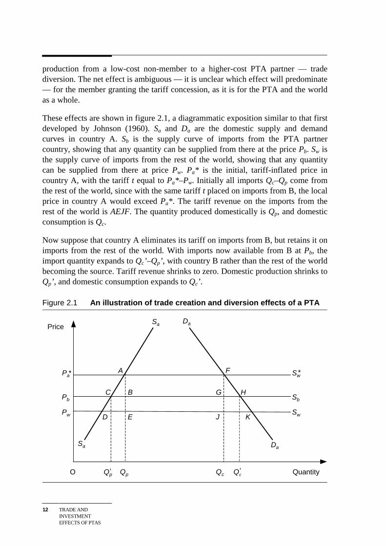
These effects are shown in figure 2.1, a diagrammatic exposition similar to that firstdeveloped by Johnson (1960). Sa and Da are the domestic supply and demandcurves in country A. Sb is the supply curve of imports from the PTA partnercountry, showing that any quantity can be supplied from there at the price Pb. Sw isthe supply curve of imports from the rest of the world, showing that any quantitycan be supplied from there at price Pw. Pa* is the initial, tariff-inflated price incountry A, with the tariff t equal to Pa*–Pw. Initially all imports Qc–Qp come fromthe rest of the world, since with the same tariff t placed on imports from B, the localprice in country A would exceed Pa*. The tariff revenue on the imports from therest of the world is AEJF. The quantity produced domestically is Qp, and domesticconsumption is Qc.
Now suppose that country A eliminates its tariff on imports from B, but retains it onimports from the rest of the world. With imports now available from B at Pb, theimport quantity expands to Qc’–Qp’, with country B rather than the rest of the worldbecoming the source. Tariff revenue shrinks to zero. Domestic production shrinks toQp’, and domestic consumption expands to Qc’.
Figure 2.1 An illustration of trade creation and diversion effects of a PTA
Price
Pa
Pb
Pw
* A
BC
D E
F
Sa
Sa
O Quantity
Da
Da
G H
J K
Sw
Sb
Sw
*
Qp Qp Qc Qc’ ’
A REVIEW OF THETHEORY OF PTAS
13
The net effect of PTA formation on economic wellbeing in country A is given byABC + FGH – BEJG. The first effect, the gain of ABC + FGH, is the net benefit toconsumers and the net resource saving in production from having domesticproduction shrink from Qp to Qp’ and consumption expand from Qc to Qc’. This isthe trade creation gain from shifting high-cost domestic production to a lower-costpartner.2 The second effect, the loss of BEJG, is that portion of the tariff revenuelost by shifting imports from the rest of the world to the higher-cost partner that isnot recouped in lower domestic prices to consumers. It is the welfare loss from tradediversion, and arises essentially because forgone domestic tariff revenue accruesinstead as profit to producers in the partner country.
The effect on country A is ambiguous a priori. If country A choses to form a PTAwith a partner that has a cost structure close to the world best, then Pb will be closeto Pw, and the height of the area BEJG will be small. But even then, if volumes oftrade are initially large relative to the net changes induced by formation of the PTA,then the width of BEJG will greatly exceed the width of ABC and FGH, and theresult could still be a net welfare loss from trade diversion. Alternatively, if trade isinitially small relative to consumption and production, then Qp and Qc will be closetogether and the width of BEJG will be small (similar to Lipsey 1958). Strictlyspeaking, only if the partner country is already at world-best production cost is awelfare gain to country A assured. But then A’s economic motive for preferentialrather than non-discriminatory trade liberalisation is unclear.
What about the welfare effects on the country receiving the preferential tariffconcession, and the effects on the rest of the world? If the simplifying assumptionsare taken seriously that both of these countries supply any quantity at a fixed price(completely elastic supply), then in the absence of other economic distortions inthese economies, the effect on their economic wellbeing is zero. Both face a changein demand for their product from country A, but because of the assumption ofconstant costs, there is no induced change in unit costs that can flow on to benefitdomestic consumers or drive an improvement in resource allocation in thosecountries.3 Thus, the effect on country A, the country granting the tariff preference,is the same as the welfare effect on the PTA and the world as a whole.
This highlights one of the key weaknesses of the simple analysis — its assumptionof constant costs of production in the partner country and in the rest of the world.The effects of relaxing these assumptions are examined shortly.
2 Viner’s (1950) original analysis omitted the consumption gain FGH. Johnson (1960) was the first
to include it as part of the gains from trade creation, thereby ending unproductive debates aboutthe possibility of welfare-increasing trade diversion (Gehrels 1957, Lipsey 1957, Michaely 1976).
3 If there is a preexisting distortion in the exporting sector of the exporting country, then anexpansion of that sector could worsen the allocation of resources.
14 TRADE ANDINVESTMENTEFFECTS OF PTAS
The simple analysis is nevertheless useful for outlining the nature of the empiricaltests for trade creation and trade diversion that are surveyed in the next chapter.Typically, these tests measure the amount by which the volume (or more often, thevalue) of trade increases with partner countries — Qc’–Qp’ in the above example —and compare it with the amount by which trade with the rest of the world is reduced— Qc–Qp in the above example. If the net effect is positive, it is still only a weaktest of whether the gains from trade creation outweigh the costs of trade diversion. Itestablishes that there is some positive width to the triangles ABC and FGH, but itdoes not establish that their areas exceed that of BEJG. This also depends on thereduction in costs per unit of newly created trade, and the increase in costs per unitof diverted trade. What can be concluded in this model is that if the empirical testsestablish net trade creation in a volume or value sense, then the PTA may still havegenerated welfare losses, but if the empirical tests establish net trade diversion, thenthe PTA cannot have created welfare gains.
Relaxing the assumption of constant costs
The assumption of constant costs in the partner country and in the rest of the worldis consistent with perfect competition in those two markets. There has been a greatdeal of analysis examining the welfare effects of instead allowing unit productioncosts to vary in those two markets, although it has not always been explicit aboutthe nature or source of the less-than-perfect competition there. More recent modelshave used product differentiation as the explicit source of market power and non-constant production costs, and are perhaps more convincing. In either case,however, the overall welfare conclusions defy simple generalisation as much asthey do in the simple case.
Terms of trade changes
Allowing unit production costs to vary and competition to be less than perfect in thepartner country and/or in the rest of the world introduces one additional source ofcomplication — the possibility of terms of trade changes for PTA partners and forthird parties, which contribute welfare effects in addition to those outlined above.Importantly, this leads to a breakdown in the one-to-one correspondence betweenthe welfare effects on the country granting the tariff preference and the welfareeffects on the PTA as a whole. Thus a PTA such as NAFTA can be beneficial as awhole, but still produce economic welfare losses for a small partner such as Mexico,as Panagariya (1999, 2000) has argued.
The easiest way to see the dramatic effects that less-than-perfect competition canhave is to imagine in figure 2.1 that the producers in country B form a cartel and
A REVIEW OF THETHEORY OF PTAS
15
‘price up’ to the world price plus external tariff after they are granted the tariffpreference. Their price would remain at Pa*, the losses to country A from tradediversion would expand to AEJF and the gains to A from trade creation woulddisappear completely! On the other hand, country B would now have a net gain inrent of ABGF that was previously tariff revenue accruing to A. The net loss to thePTA and the world as a whole would be BEGJ. Thus, less-than-perfect competitioncan preserve the losses from trade diversion but destroy the gains from tradecreation.
But even this conclusion is not completely robust. Panagariya (2000) shows how theanalysis of the previous paragraph assumed implicitly that after the formation of thePTA, country B maintained an external tariff equal to the pre-union tariff of A. Thissituation, where each country adopts a common external tariff, is known as acustoms union. If instead, each country retains its initial tariff, the PTA is a freetrade area. Panagariya (2000) shows that with less-than-perfect competition, thewelfare effects of a free trade area on country A and the PTA as a whole cansometimes (depending on initial production and trade shares) be ambiguous ratherthan negative, although the effect on B remains positive.
Panagariya (2000) also analyses several other special cases at length, someinvolving less-than-perfect competition in the rest of the world as well as in thepartner country. He also discusses the case where product differentiation is thesource of market power and less-than-perfect competition. While none of thesecases can claim full generality, the analysis that comes closest is that of Mundell(1964). Riezman (1979) is another early contribution. Panagariya (2000) argues thateven the later, differentiated products analysis is a special case of Mundell’s earlierwork.
Mundell (1964, p. 8) draws the following more general conclusions on the effects ofa customs union, assuming that all goods are gross substitutes and initial tariffs arelow:
(1) The discriminatory tariff reduction by a member country improves the terms oftrade of the partner country with respect to both the tariff reducing country and the restof the world, but the terms of trade of the tariff-reducing country might rise or fall withrespect to third countries.
(2) The degree of improvement in the terms of trade of the partner country is likely tobe larger the greater is the member’s tariff reduction; this establishes the presumptionthat a member’s gain from a free-trade area will be larger the higher are initial tariffs ofpartner countries.
A key to this result is the revenue transfer effect that can arise with less-than-perfectcompetition. It is also the basis for Panagariya’s conclusion that the United States is
16 TRADE ANDINVESTMENTEFFECTS OF PTAS
likely to gain, but that Mexico could lose, from NAFTA. Existing empirical tests ofthe effects of NAFTA are discussed in the next chapter.
Economies of scale
A final theme in the policy arena has been the possibility of gains to PTA formationarising from economies of scale. This was part of the rationale for the PTAsproposed among developing countries in the 1960s, and the argument has appearedfrequently in policy circles since. Corden (1972) showed that economies of scaledid not establish a stronger presumption in favour of PTAs being welfare improvingthan was the case under constant or increasing costs. While economies of scaleprovide an additional source of gain — a cost reduction effect as existing firmsexpand and unit production costs are lowered — they also provide an additionalsource of loss — a trade suppression effect as more expensive (but now viable)domestic production replaces cheaper imports from third countries. It is also true inCorden’s model that the PTA members could do better by liberalising unilaterallyor on non-discriminatory basis, as was the case under constant costs.
Baldwin and Venables (1995) explore further the pro-competitive cost reducingeffects of PTAs under imperfect competition and increasing returns to scale. Theyconclude that if PTA formation changes firm behaviour so that markets become lesssegmented and more integrated, there could be substantial pro-competitive gains.
The World Bank (2000) notes, however, that most of the efficiency gains fromopenness come from reductions in production inefficiencies, rather than from scaleeffects. They also note that estimates from the EU found that pro-competitiveeffects were largest, not in markets where there was a high level of intra-EU trade,but instead in markets where there was a high degree of competition from firmsoutside the union. They conclude that while there is potential for gains fromcompetition and scale effects in industrial sectors of the economy, achieving themmight require ‘deep integration’ policies — removing not just tariff barriers, butalso ‘trade chilling’ contingent protection, and other frontier frictions such asfrontier red tape and differences in national product standards. They also note thatthese gains may also be achievable through unilateral trade liberalisation.
A REVIEW OF THETHEORY OF PTAS
17
Intermediate goods and rules of origin
The above analysis also simplifies by ignoring production and trade in intermediategoods, and the effects that rules of origin can have on this trade. The literature onrules of origin is sparse, but the following points have been made.4
• In the absence of traded intermediate inputs, rules of origin have anunambiguously harmful effect. Without them, a free trade area would operatelike a customs union, with the lowest tariff among members being the externaltariff. Rules of origin generate additional trade diversion.
• With traded intermediate inputs, rules of origin could reduce trade diversion.This can happen if rules of origin require a producer to purchase inputs from amore expensive member source in order to qualify for a tariff concession onoutput. This can reduce the amount of trade diversion in the final product.
• But for the same reason, rules of origin can also counteract trade creation.
• In intermediate goods production, rules of origin are likely to encourage tradediversion and thus be harmful.
Thus rules of origin can transmit the trade diversion associated with preferentialliberalisation back up the production chain.
General conclusions from static analysis?
The above analysis shows that some of the generalisations that are sometimes madeabout the static effects of PTAs should be viewed with caution.
For example, it is sometimes claimed that the static gains will be greater, the largerthe trade barriers being reduced (Laird 1999). As the above analysis shows,however, it cannot be presumed that the gains will flow to the country with thosehigh tariffs initially (as would be the case with non-preferential trade liberalisation).Instead, the analysis using less-than-perfect competition suggests the opposite.
Similarly, it is sometimes claimed that the gains will be higher, the higher the shareof pre-existing trade between partners. This is one basis for the claim that there willbe gains to PTAs among ‘natural trading partners’, a claim originating withWonnacott and Lutz (1989). The reasoning is that there is not much trade with therest of the world that can be diverted. Bhagwati and Panagariya (1999) give adetailed critique of this proposition. Among the points they make are the following:
4 For analyses of the welfare effects of rules of origin, see Duttagupta and Panagariya (2002), Ju
and Krishna (1998), Krishna and Krueger (1994) and Krueger (1999b). The following summaryis drawn from Panagariya (1999).
18 TRADE ANDINVESTMENTEFFECTS OF PTAS
• the proposition is neither symmetric nor transitive — the United States isMexico’s largest trading partner, but the reverse is not true, and while the UnitedStates is also Canada’s largest trading partner, Mexico and Canada have littletrade with each other;
• the welfare effects of PTAs depend on the volumes of trade actually diverted,which need not be proportional to initial trade shares;
• in this respect, Lipsey’s (1958) observation about the importance of importsfrom either source relative to domestic consumption may have more force, buteven here, the relative cross-price elasticities of each import with the home goodalso matter.
A second variant of the ‘natural trading partner’ hypothesis is that PTAs are morelikely to be beneficial when they are among geographic neighbours, again becauseintra-bloc trade is likely to be large initially. Bhagwati and Panagariya (1999) pointout that although gravity equations (used in empirical tests of the gains from PTAs,and discussed more fully in subsequent chapters) show that there is an inverserelationship between distance and trade volumes, once other factors such as sizeand relative income levels are controlled for, there is no simple correlation betweendistance and trade volumes that would support this natural trading partnerhypothesis.
A final variant of the ‘natural trading partner’ hypothesis is that PTAs are morelikely to be beneficial when they are among geographic neighbours, becausetransport costs will be lower. Bhagwati and Panagariya (1999) construct acounterexample showing that the efficient policy choice of a preferential tradingpartner among countries with basically the same supply characteristics can beparadoxically the more distant. This is because transport costs can make the supplyfrom the distant partner more price responsive (elastic), and efficient pricediscrimination requires a lower tax (via the PTA) on the more elastic supply.
It is also claimed that trade creation and welfare gains will be larger, the larger thepartner country, the more diversified the partner country’s economy and the closerits prices resemble world prices (Laird 1999). The first two of these criteria appearto be proxies for the third, but as the above analysis under both perfect and less-than-perfect competition shows, having a partner’s price ‘close to’ the world bestprice may not be enough to prevent large losses from trade diversion, especially ifproducers in the partner country ‘price up’ to the external tariff.
Pomfret (1997, p. 174) claims:
Within the mainstream theory there is little scope for expecting the welfare impact onoutsiders to be non-negative, although the order of magnitude is an empirical matter.
A REVIEW OF THETHEORY OF PTAS
19
Non-participants will be affected primarily by terms of trade effects. The quotefrom Mundell above shows that from the outsider’s perspective, its terms of trademay rise against the tariff-reducing country, although they will fall against itspartner country, so even net losses to outsiders are not a sure thing in an asymmetricPTA (where only one partner lowers tariffs). They are much more likely in asymmetric PTA.
Pomfret (1997) also points out that in the simple case of constant costs, there was aclear policy prescription — avoid introducing the second policy distortion andliberalise on a non-discriminatory basis. It was this observation that led someanalysts (Johnson 1965, Cooper and Massell 1965) to conclude that preferentialtrading arrangements could be explained only by non-economic motives. But withnon-constant costs and less-than-perfect competition, even this presumptiondisappears:
Mundell (1964) identified realistic situations where all GDA [geographicallydiscriminatory arrangement] member countries could improve their terms of trade withthe rest of the world, with all participants benefiting in a manner that would not bereplicated by MFN tariff reductions, although clearly this is at the expense of countriesoutside the GDA and is possibly welfare-reducing for the world as a whole. (Pomfret1997, p. 204)
The one general conclusion that can be drawn from the static analysis is that it hasproved extremely difficult for analysts to come up with robust ‘rules of thumb’ tocharacterise situations where the gains from trade creation will exceed the lossesfrom trade diversion, so that PTAs will deliver gains to members and to the worldas a whole. This suggests that it will be equally difficult for governments to identifyreal-world PTA opportunities that meet this criterion. It also means that it will bedifficult, at least on static grounds, for WTO member countries to identify robustnew WTO disciplines on PTA formation that will minimise the possibility of lossesto either PTA members or third parties.5 The scope for designing such rules isexamined on political economy grounds briefly in the next section.
Other static arguments in favour of PTAs
The Kemp-Wan (1976) theorem offers the tantalising prospect of designing an PTAthat can benefit at least one member, without harming other members or outsideparties.
5 Pomfret (1997) and Panagariya (2000) note how volume-based rules of the sort proposed by
McMillan (1993) can be confounded by terms of trade effects.
20 TRADE ANDINVESTMENTEFFECTS OF PTAS
The key insight is that a second policy instrument is required to undo the damagedone by increasing the geographic dispersion in tariffs. That instrument is theexternal tariff. Instead of setting a common external tariff equal to members’average initial tariff, members of a customs union should reduce that external tariffby enough to ensure no change in the net trade of members with the rest of theworld. This ensures no harm to the rest of the world. To ensure that no unionmember is harmed, there also need to be appropriate compensation paymentsamong members.6
But therein lies the problem — by how much should the external tariff fall, andwhat are the compensation payments required? The theorem is an existenceproposition, rather than a policy prescription.
What is worse, several papers (Grossman and Helpmann 1995, Panagariya andFindlay 1996) show that, once political economy considerations are recognised, thepolitical incentives are for PTAs to be formed precisely when they are most tradediverting, and for external tariffs to be raised rather than lowered. Clearly, politicaleconomy considerations have a role to play in assessing PTAs.
2.2 The dynamic effects of PTAs on multilateralliberalisation
Building blocks or stumbling blocks?
A convincing answer to the question of whether PTAs are building blocks orstumbling blocks to multilateral trade liberalisation requires a political economyfocus. What are the incentives for countries to want to enter an existing PTA? Whatare the incentives for existing members to allow new entry? And what are theincentives for new or existing members to continue to seek multilateral tradeliberalisation?
Several papers have avoided these questions by simply assuming that a PTAexpands its membership. They then assess whether that will increase or reducewelfare. The most famous was the paper by Krugman (1993), which outlined a setof circumstances in which world welfare would first fall, and then rise, as the worldwas divided into fewer, larger trading blocks. World welfare was at its lowest whenthe number of trading blocks was three!
6 Panagariya and Krishna (2002) prove a similar result for free trade areas.
A REVIEW OF THETHEORY OF PTAS
21
Krugman’s analysis has been shown to be sensitive to his model’s assumptions(Srinivasan 1993, Deardorff and Stern 1994). For example, Deardorff and Sternshow instead that when trade is motivated by differences in factor endowments, asin many conventional trade models, world welfare rises monotonically with the sizeof the blocks.
Four key papers have examined the incentives for PTA membership to expand. Twoargue that PTAs will be stumbling blocks, by reducing the incentives of members toseek multilateral trade liberalisation. A third paper argues that there are incentivesfor non-members to seek entry into PTAs in domino fashion, until the whole worldis covered. A fourth paper shows that there are incentives for existing members toprevent such an outcome.
In Krishna (1998), governments respond to lobbying by firms. In this oligopolisticcompetition model, the bilateral PTA reduces the incentives of members toliberalise tariffs reciprocally with non-member countries, and with sufficient tradediversion, this incentive could be reduced enough to make impossible an initiallyfeasible multilateral trade liberalisation.
In Levy (1997), governments instead respond to the will of the median voter. In aricher model with scale economies and product variety, bilateral PTAs canundermine political support for multilateral free trade. What is worse, a benignimpact is impossible — if a multilateral free trade proposal is not feasible in theabsence of a PTA, it will not become feasible with the PTA.
In the third paper, Baldwin (1996) considers only the incentive of non-members tojoin a PTA, and argues that there will be a positive ‘domino’ effect. The PTAimplies a loss of cost competitiveness by imperfectly competitive non-memberfirms, whose profits in the PTA market decline because of the tariffs they still face.These firms lobby for entry, tipping the political balance towards entry in the non-member countries closest to the margin. This new entry sets up its own cycle of newcost pressures and further lobbying for entry.
Baldwin (1996) does not consider the incentives for existing members to allow newentrants into the PTA. Zissimos and Vines (2000) acknowledge that joining a PTAis the best safe-haven strategy when other countries are doing so. But they arguethat the same terms of trade changes that encourage non-members to seek entry arethe factors that will eventually discourage existing members from allowing it —terms of trade gains to members require there to continue to be some non-members
22 TRADE ANDINVESTMENTEFFECTS OF PTAS
to exploit in this fashion.7 PTA block formation will fall short of multilateral freetrade.8 They show how the provisions in Article XXIV that prevent an increase inexternal tariffs are not sufficiently strong to prevent terms of trade changes inducedby internal tariff reduction à la Mundell, the key to their result. For the same reason,block members would not be induced to accept ‘open regionalism’ as an alterativemultilateral discipline, whereby any trade block must be open to the membership ofany country that wants to join.
Thus the bulk of the existing literature seems to point to PTAs being stumblingblocks rather than building blocks to multilateral liberalisation. That said, the paperof Zissimos and Vines (2000) shows that for plausible parameters, worldequilibrium could involve one block being large — about 90 per cent of the worldeconomy.9 Perhaps this is not too dissimilar to the current WTO membership. Butthey also note that any attempt to tighten the WTO rules on PTA formation willneed to recognise that at least some current PTA members are better off than theywould be under global free trade. This dynamic makes the prospects for successfulredesign of the rules difficult.10
Other dynamic arguments in favour of PTAs
Bhagwati (1999) evaluates the arguments heard in policy circles that regionalism isa quicker, more efficient or more certain route to free trade than multilateralnegotiation.
On the question of speed, he notes that even now, the European Union has still notfully achieved its pledge to eliminate internal trade barriers, as required by ArticleXXIV. He also notes that PTAs have been no more successful than multilateralforums at tackling the hard cases such as agriculture and textiles. Indeed, Hoekmanand Leidy (1993) find that the holes (areas left out) and loopholes (areas where thedisciplines of free trade are avoided) are virtually identical in either case.
7 Zissimos and Vines (2000) is a further development of the arguments about negative externalities
from terms of trade changes developed by Bond and Syropoulos (1996) and Bagwell and Staiger(1998, 1999), among others.
8 Freund (2000) shows that this argument may not be robust to the presence of sunk costs, becausethen ‘first movers’ gain a permanent advantage from PTA formation that persists in a subsequentmove to free trade, albeit at the expense of non-members.
9 Andriamananjara (1999) has a similar theoretical finding, but finds that the larger block would beabout two-thirds of the world economy.
10 Lloyd (2002) argues that bilateral ‘hub and spoke’ arrangements can be beneficial because theycircumvent the unanimity rule presumed by Zissimos and Vines (2000). But this presupposes thatpreexisting spoke partners will stand silent as new bilateral spoke arrangements are negotiated,even ones that disadvantage preexisting spokes.
A REVIEW OF THETHEORY OF PTAS
23
On the question of efficiency, or the ability to ‘deliver the goods’, Bhagwati notesthat the concessions that hegemons may be able to extract from smaller tradingpartners in a regional forum may not exactly be in the best interests of those smallerpartners or the world as a whole, and may distort multilateral negotiations.
As is now widely conceded among economists, the case for TRIPS [the agreement onprotection of trade-related intellectual property rights under the WTO] for instance isnot similar to the case for free trade: there is no presumption of mutual gain, worldwelfare itself may be reduced by any or more IP protection, and there is little empiricalsupport for the view that ‘inadequate’ IP protection impedes the creation of newtechnical knowledge significantly. Yet the use of US muscle, unilaterally through‘Special 301’ actions, and the playing of the regional card through the NAFTA carrotfor Mexico, have put TRIPS squarely and effectively into the MTN. (Bhagwati 1999,p. 24)
On the question of certainty, and the ability of PTAs to lock in a reformcommitment, Bhagwati notes that multilateral forums also create commitments —tariffs are bound, and the WTO sanctions retaliatory action against members whoraise their tariffs above bound levels. He also notes that WTO disciplines on PTAsare lax, creating incentives to negotiate ‘second best’ PTAs. PTAs have also beenknown to fail or stagnate.
2.3 The effects of non-trade provisions of PTAs
So far, the discussion has been about the tariff provisions of PTAs, and the effectsof those provisions on merchandise trade. Despite the evolution of third wave ornew age agreements, there has been little literature dealing with the effects ofpreferential non-tariff provisions.
One exception is Pomfret (1997, chapter 10). He discusses three types of non-border measures — foreign direct investment policy, competition policy andmonetary integration. He notes that PTAs may contain preferential provisions inthese areas designed to be discriminatory, or PTAs may simply present regionalforums for negotiating geographically limited harmonisation when global regimesare unattainable.
• On investment, he concludes that investment provisions can be used asdiscriminatory protective devices, so that a preferential agreement that balancedthe interests of like-minded countries may not be in the interests of the rest of theworld — if a global investment code is desired, it should be designed by a globalrather than regional body.
• On competition policy, he concludes that the case for preferential ordiscriminatory competition policy is weak, but there are arguments for
24 TRADE ANDINVESTMENTEFFECTS OF PTAS
harmonising competition policies to reduce sources of international tension, andit may be easier to do this in a regional setting.
• On monetary integration, he concludes that the relationship between monetaryintegration and regional integration is weak, and at the level of most PTAs,monetary union is relatively unimportant.11
The welfare effects of preferential investment provisions
Pomfret (1997) does not discuss in detail the economic welfare effects ofdiscriminatory provisions governing foreign direct investment, but his discussion ofthe welfare effects of preferential non-tariff barriers to trade is suggestive. Thereason is that work at the Productivity Commission has shown how barriers to theestablishment and operation of foreign multinationals can be modelled as non-tariffbarriers on the flow of capital, and the output of FDI firms once established,respectively (Dee and Hanslow 2001, Dee, Hanslow and Phamduc 2003).
Pomfret (1997) notes that the critical distinction is whether non-tariff barriers arerent-generating — allowing a markup of price over cost — or whether they are cost-escalating — increasing the real resource costs of doing business.12
If they are rent-generating, then they operate much like tariffs, except that the rentsstay in the hands of importers or exporters rather than accruing to government in theform of tariff revenue. If non-tariff barriers are of this form, then preferentialliberalisation will have similar effects to preferential tariff liberalisation. There willbe welfare gains from trade creation where rents are reduced, and there will bewelfare losses from trade diversion on that trade where rents still accrue.13
If instead non-tariff barriers are cost-escalating, then liberalisation unambiguouslysaves real resources. As Baldwin (1994) has shown, in this situation preferentialliberalisation is always welfare-increasing, whether or not the trade partner is theleast-cost supplier.14
11 Frankel (1997) and Rose (2000), summarised in the next chapter, reach a different conclusion.12 Dee (2001) shows that the same distinction is critical for the welfare effects of barriers to
services trade.13 Pomfret (1997) acknowledges that there are situations (eg imperfect competition, uncertainty)
where this equivalence between tariffs and rent-generating non-tariff barriers breaks down.14 The unambiguous gains from removing cost-escalating non-tariff barriers (eg undertaking trade
facilitation) have also been stressed in studies of the effects of deep integration, such as Emersonet al. (1988) and Lawrence (1997).
A REVIEW OF THETHEORY OF PTAS
25
The analogy with preferential liberalisation of investment provisions can now bedrawn.
• If investment barriers are of the sort to generate rents, then preferentialliberalisation will generate gains from investment creation, as production ismoved from a high-cost domestically-owned producer to a lower-cost member’saffiliate. But it will also generate losses from investment diversion, asproduction is moved from a low-cost non-member affiliate (located somewherein the world) to a higher-cost member affiliate.
• If investment barriers are of the sort to escalate costs, then preferentialliberalisation will unambiguously save real resources and increase welfare.
Thus the welfare implications are more positive than with preferential tariffliberalisation, because of the possibility of saving real resources. But the potentialfor losses from investment diversion also remains.
The welfare effects of investment responding to preferential tradeprovisions
In a series of papers, Ethier (1998a, b, 1999, 2001) develops variants of a model inwhich investment responds in ‘beachhead’ fashion to the preferential tradeprovisions of PTAs.
This model is an explicit attempt to capture some of the salient features of thirdwave PTAs. He observes that many third wave agreements are between small,‘outside’ countries that are not yet members of the world trading system,15 andlarger, ‘inside’ countries that are. The small, outside countries want to reform theirinternal economies so that they can be accepted as members of the global tradingsystem. Ethier asserts that the sign of successful reform is whether these countriesattract foreign direct investment.16 Their problem is how to signal a crediblecommitment to reform in advance.
The outside country’s solution is to sign an PTA with an inside country involvingenough trade concessions to the inside country so that it in turn will have anincentive to act as an enforcer and retaliate if the outside country deviates from itsreform commitment. But the aim is not necessarily to receive enormous concessions
15 Ethier (2001) identifies these as countries that until recently adopted basically-autarkic,
antimarket policies. The issue is not membership of the WTO per se.16 Blustein’s (2001) account of how the ‘electronic herd’ responded to IMF reform programs in the
Asian crisis countries suggests that while there may be some truth to Ethier’s assertion, therelationship between reform programs and investment behaviour is more complex than Ethiersuggests.
26 TRADE ANDINVESTMENTEFFECTS OF PTAS
from the inside country in return. All that is required is a small trade concession, sothat multinationals have an incentive to locate in the outside country and to use it asa beachhead for trade to the inside country. Thus Ethier also explains the recentphenomenon of some third wave agreements being asymmetric:
What matters here is what the small reforming country gives, in terms of tradeconcessions, not what it gets, because it is the former which influences the likelihood ofretaliation by the partner in the event of backsliding. The external commitment in turnmakes the country more attractive for direct investment, relative to similar countrieswithout such external commitments. (Ethier 1998b, p. 1157)
Note too that there is no presumption that the investment comes from the large PTApartner.
The goal is to compete with other similar countries for direct investment, not to expandgreatly exports to their partners or to attract from them investments that wouldotherwise not be made at all. Such ‘investment creation’ will be modest at best. (Ethier1998b, p. 1158)
Ethier (2001) also examines in detail the incentives of the large inside country toaccede to such an arrangement, even in preference to pursuing further multilateralreform.
Finally, he shows that a world equilibrium in which small countries compete forinvestment in this fashion is beneficial, because it internalises an externality. Theglobal interest calls for successful reform to be as widespread as possible, but ifthere are agglomeration economies, then multinationals will want to cluster theirforeign investments together. A global web of bilateral PTAs, initiated by outsidecountries’ competition for investment, internalises the externality.
Ethier’s positive outlook on PTA formation comes from this benign view ofcompetition for investment, rather than from the characteristics of PTAs per se. Ashe acknowledges, his model of PTA formation is consistent with massive amountsof investment diversion to take advantage of trade beachheads, and subsequent tradediversion from those beachhead positions. But in his model, there is sufficientsymmetry between countries for this trade and investment diversion to have noadverse welfare consequences — every country is the ‘lowest cost’ source ofimports and the ‘best’ host for FDI. With more diversity, this massive diversion isno longer benign.
Ethier’s positive view also depends on the competition for investment occurringthrough reform, which is seen as a ‘good thing’. If it were to occur through thecompetitive granting of investment incentives, or if ‘reform’ involved inappropriateconcessions forced by a larger hegemon (as Bhagwati fears), the competition forinvestment may itself be less benign.
A REVIEW OF THETHEORY OF PTAS
27
2.4 Summary
The first wave of PTAs coincided with a theoretical examination of the static effectson trade flows and economic well-being in member and non-member countries. Thesimple analysis with constant costs led to the conclusion that because PTAs easeone economic distortion, but exacerbate another, gains to PTA members are notassured. The more recent analysis with non-constant costs confirms this finding. Italso suggests that because of the redistributive effects of less-than-perfectcompetition, individual PTA members need not gain, even when the PTA is goodfor the membership as a whole. And the losers will tend to be those members withhigh tariffs initially.
The second wave of PTAs spurred an examination of whether PTA formation was abuilding block or a stumbling block to multilateral trade liberalisation. The mostconvincing analyses were those that examined the incentives for non-members tojoin a PTA, and for existing members to allow that expansion. The most recent,comprehensive analysis finds that since PTA membership confers a terms of tradegain to members at the expense of non-members, at least some members will bebetter off limiting PTA membership than allowing expansion to cover the world as awhole. Any redesign of the WTO rules disciplining the formation of PTAs wouldneed to recognise that reality.
The third wave of PTAs has begun to spur analyses of the non-tariff provisions ofPTAs. At first sight, the focus of third wave agreements on non-tariff issues maysuggest that traditional concerns about trade diversion are outmoded. But a closerlook suggests otherwise. Investment barriers can be used as a protective device, andpreferential liberalisation of investment provisions can generate investmentdiversion, with adverse consequences, as well as beneficial investment creation.Even where investment is attracted in ‘beachhead’ fashion in response to tradeliberalisation provisions, both the investment and subsequent trade from thebeachhead position may be diversionary. Thus the non-tariff focus of third waveagreements cannot shake the first wave concerns about the adverse second-besteffects of preferential liberalisation.

28 TRADE ANDINVESTMENTEFFECTS OF PTAS
REVIEW OF THEEXISTING EMPIRICALEVIDENCE
29
3 Review of the existing empiricalevidence
Each wave of PTAs has brought a specific focus to empirical analysis.
• In response to the first wave, the empirical focus was to estimate the static grosstrade creation and trade diversion effects of PTAs. Empirical studies used eitherex ante or ex post techniques.
• In response to the second wave, PTAs were assessed as building or stumblingblocks according to their net trade creation or diversion effects. These studiesincreasingly used analytical and ex ante techniques.
• The empirical analysis of third wave issues is still in its infancy. A few studieshave provided analytical insights into the effects of trade provisions oninvestment. Little attention has yet been paid to non-trade provisions.
This chapter assesses the empirical evidence on static trade creation and tradediversion — the issue that drove the first wave. It has remained a preoccupation ofempirical research even with the second and third waves.
The different approaches used to estimate trade creation and diversion effects arediscussed in the next section, followed by more in-depth discussion of the gravitymodel, the key econometric method used. The chapter then reviews the findings onthe trade creation and diversion effects of PTAs. A brief summary is also given ofthe evidence on second and third wave issues.
3.1 Approaches to assessing PTAs
The key empirical task is to disentangle the effects of a PTA from other changes inan economy. There are two main approaches.
First, ex ante studies have used counterfactual analyses based on partial or generalequilibrium models. These models assume a certain model structure, with specificfunctional forms and parameter values to represent the countries in a base year priorto the formation of the PTA. Those models with a sufficiently tight theoreticalstructure are also able to be used to draw direct inferences about welfare. The modelis then subjected to the preferential removal of tariffs alone, and the welfare effects
30 TRADE ANDINVESTMENTEFFECTS OF PTAS
are calculated. Surveys of assessments of PTAs using general equilibrium modelscan be found in De Rosa (1998) and Robinson and Thierfelder (2002). Scollay andGilbert (2000) survey CGE assessments of APEC. Most of these studies find thatPTAs create additional trade for both members and non-members. Most also findthat PTAs improve welfare, at least among member countries.
However, these CGE analyses suffer from a number of theoretical and practicaldifficulties. Some (in particular, many of those covered by the Robinson andThierfelder survey) assume fixed terms of trade. As noted by Panagariya andDuttagupta (2002), this is inconsistent with one of their other key assumptions,namely, product differentiation at the national level. Deardorff and Stern (1994)note how the assumption of national product differentiation can itself leave an‘idiosyncratic stamp’ on examinations of PTAs, in particular helping to explainKrugman’s (1993) finding of welfare losses in a world of three trading blocs, aresult that does not appear to carry over to empirical CGE analyses. But in addition,the assumption of fixed terms of trade rules out one of the key effects of PTAs,namely, terms of trade changes.
Further, the CGE studies typically use a very simple characterisation of PTAs. Mostassume comprehensive across-the-board elimination of tariffs (and sometimes non-tariff barriers) among members, although most real-world PTAs have complexpatterns of exemptions. In addition, the studies typically ignore many of thepotentially trade-restrictive non-tariff measures, such as rules of origin or localcontent requirements, that typically accompany the merchandise trade measures.Finally, they typically ignore provisions affecting non-merchandise trade (althougha notable exception is Hertel, Walmsley and Itakura 2001).
This is not to deny that particular CGE models, when used with appropriateassumptions (such as variable terms of trade), can give valuable insights into thepossible effects of important tariff provisions of PTAs. But conclusions drawn fromsurveys of CGE studies should be treated cautiously. And the results from CGEstudies should not be generalised to draw conclusions about the effects of non-merchandise trade provisions of PTAs.
By contrast, ex post studies of PTAs measure their trade creation and tradediversion effects by using econometric methods to establish a link between actualPTA formation and actual trade outcomes, controlling for the effects of all otherinfluences. Since welfare is unobservable, these econometric studies cannotestablish welfare effects directly. And as noted in the previous chapter (p. 14), thelink between trade outcomes and welfare is weak. But the studies do examine actualPTAs, in all their complexity, including non-merchandise trade provisions.
REVIEW OF THEEXISTING EMPIRICALEVIDENCE
31
The present study focuses on these ex post evaluations of the effects of PTAs. Theex ante studies typically look only at the tariff provisions of PTAs (and then onlyimperfectly), so they do not evaluate the third wave aspects discussed in chapters 1and 2. By contrast, the ex post studies of actual PTAs include the actual responses toany third wave provisions embodied in them. The remainder of this chapter looks atthe existing evidence, while the following two chapters present new evidence on theex post effects of tariff and non-tariff provisions, respectively.
Gravity model
The gravity model is the key ex post econometric technique used to examine thedeterminants of bilateral trade flows. It is a model of trade flows based on ananalogy with the law of gravity in physics. Trade between two countries ispositively related to their size, and inversely related to the distance between them. Anumber of other explanatory variables are added to this model to analyse variousbilateral trade policy issues. In the augmented gravity model, trade between twocountries is determined by supply conditions at the origin, demand conditions at thedestination, and various stimulating or restraining forces. This specification hasrecently been shown to be consistent with a number of theoretical models ofinternational trade.1
The standard way of assessing the impact of PTAs is to add PTA-specific binarydummy variables to the augmented gravity model to capture effects not capturedthrough normal bilateral trade determinants.
PTA specific dummy variables
Studies adding PTA-specific dummy variables to capture the trade creation anddiversion effects of PTAs date back to the 1970s. Aitken (1973) initially added onedummy variable to his gravity model to capture the intra-bloc effect of a PTA — the‘gross trade effect’ of Balassa (1967).
Bayoumi and Eichengreen (1995) and Frankel (1997) added two dummy variablesfor each PTA to capture the separate effects on intra-bloc and extra-bloc trade. The‘net trade effect’ of Viner (1950) can be obtained by combining these two dummy
1 The gravity model is derived theoretically as a reduced form from a general equilibrium model of
international trade in goods. Baier and Bergstrand (2001) derived it from a model of monopolisticcompetition. Feenstra, Markusen and Rose (2001) derived it from a reciprocal dumping model oftrade with homogeneous goods. Deardorff (1998) derived it from a model with perfectlycompetitive markets. Evenett and Keller (1998) showed empirically that the monopolistic-competition based theory of trade fits the trade flows among industrialised countries well.
32 TRADE ANDINVESTMENTEFFECTS OF PTAS
variables to assess whether an increase in intra bloc trade has come at the expenseof lower extra bloc trade. The size, sign and the significance of the PTA-specificdummy coefficients has also been used to indicate whether a PTA is a building orstumbling block to multilateral trade liberalisation — the second wave issue.
The first dummy variable takes a value of one when the two countries are membersof the same PTA. The second dummy variable is one if either country in a particularpair belongs to the PTA. A positive coefficient on the first dummy variableindicates that members of a PTA trade more with each other than would bepredicted by their normal bilateral trade determinants and the average behaviour ofcountries in the sample. In other words, a positive coefficient on the first dummyvariable indicates that the formation of a PTA enhances intra-bloc trade. The seconddummy variable measures the extent of additional trade between an PTA memberand a non-member, relative to what the gravity model predicts for a random pair ofcountries that do not belong to that particular PTA. A negative and significantcoefficient for the second dummy variable suggests that the PTA leads to tradediversion.
If a positive coefficient on the first dummy exceeds a negative coefficient on thesecond, then trade creation may be said to outweigh trade diversion. But as noted inchapter 2, the effects of the PTA on welfare do not follow immediately. These alsodepend on the reduction in costs per unit of newly created trade, and the increase incosts per unit of diverted trade. They also depend on terms of trade effects, whichare not captured at all in this type of analysis (although their direction at least canoften be inferred from the changes in directions of trade).
Soloaga and Winters (2001) added three dummy variables for each PTA, todistinguish an intra-bloc effect, an extra-bloc effect on imports and an extra-bloceffect on exports (see figure 3.1). The second and third dummy variables in theirstudy measure the extent of import diversion and export diversion, respectively.They argued that both are needed because bloc members’ imports and exports couldfollow different patterns after the formation of a PTA.
As noted, the ‘net trade effect’ of a PTA has been used as a tentative indicator toassess the second wave issue — whether a PTA is a building or stumbling block tofree trade. Frankel (1997) used the sum of the significant intra-bloc and extra-bloceffects obtained from his gravity model to infer the second wave issue. Thiscriterion will be discussed further in section 3.3.
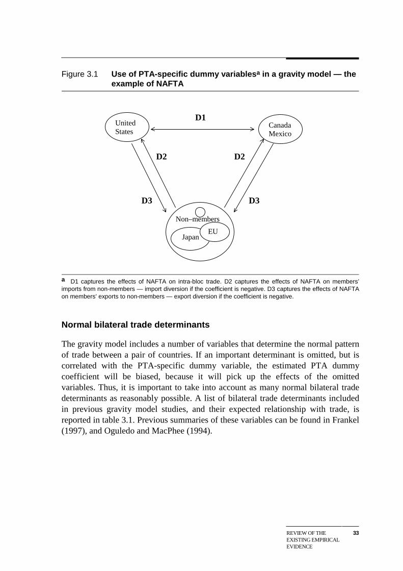
REVIEW OF THEEXISTING EMPIRICALEVIDENCE
33
Figure 3.1 Use of PTA-specific dummy variablesa in a gravity model — theexample of NAFTA
a D1 captures the effects of NAFTA on intra-bloc trade. D2 captures the effects of NAFTA on members’imports from non-members — import diversion if the coefficient is negative. D3 captures the effects of NAFTAon members’ exports to non-members — export diversion if the coefficient is negative.
Normal bilateral trade determinants
The gravity model includes a number of variables that determine the normal patternof trade between a pair of countries. If an important determinant is omitted, but iscorrelated with the PTA-specific dummy variable, the estimated PTA dummycoefficient will be biased, because it will pick up the effects of the omittedvariables. Thus, it is important to take into account as many normal bilateral tradedeterminants as reasonably possible. A list of bilateral trade determinants includedin previous gravity model studies, and their expected relationship with trade, isreported in table 3.1. Previous summaries of these variables can be found in Frankel(1997), and Oguledo and MacPhee (1994).
D2D2
D3 D3
D1UnitedStates
JapanEU
Non–members
CanadaMexico
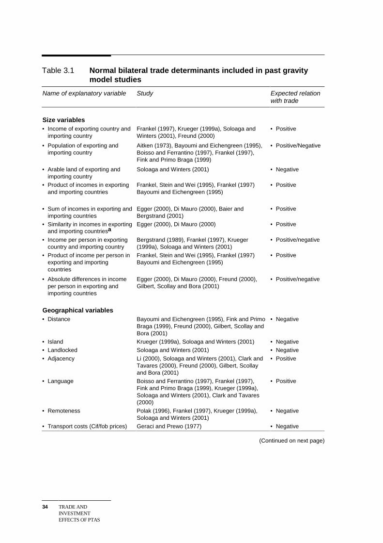
34 TRADE ANDINVESTMENTEFFECTS OF PTAS
Table 3.1 Normal bilateral trade determinants included in past gravitymodel studies
Name of explanatory variable Study Expected relationwith trade
Size variables• Income of exporting country and
importing countryFrankel (1997), Krueger (1999a), Soloaga andWinters (2001), Freund (2000)
• Positive
• Population of exporting andimporting country
Aitken (1973), Bayoumi and Eichengreen (1995),Boisso and Ferrantino (1997), Frankel (1997),Fink and Primo Braga (1999)
• Positive/Negative
• Arable land of exporting andimporting country
Soloaga and Winters (2001) • Negative
• Product of incomes in exportingand importing countries
Frankel, Stein and Wei (1995), Frankel (1997)Bayoumi and Eichengreen (1995)
• Positive
• Sum of incomes in exporting andimporting countries
Egger (2000), Di Mauro (2000), Baier andBergstrand (2001)
• Positive
• Similarity in incomes in exportingand importing countriesa
Egger (2000), Di Mauro (2000) • Positive
• Income per person in exportingcountry and importing country
Bergstrand (1989), Frankel (1997), Krueger(1999a), Soloaga and Winters (2001)
• Positive/negative
• Product of income per person inexporting and importingcountries
Frankel, Stein and Wei (1995), Frankel (1997)Bayoumi and Eichengreen (1995)
• Positive
• Absolute differences in incomeper person in exporting andimporting countries
Egger (2000), Di Mauro (2000), Freund (2000),Gilbert, Scollay and Bora (2001)
• Positive/negative
Geographical variables• Distance Bayoumi and Eichengreen (1995), Fink and Primo
Braga (1999), Freund (2000), Gilbert, Scollay andBora (2001)
• Negative
• Island Krueger (1999a), Soloaga and Winters (2001) • Negative• Landlocked Soloaga and Winters (2001) • Negative
• Adjacency Li (2000), Soloaga and Winters (2001), Clark andTavares (2000), Freund (2000), Gilbert, Scollayand Bora (2001)
• Positive
• Language Boisso and Ferrantino (1997), Frankel (1997),Fink and Primo Braga (1999), Krueger (1999a),Soloaga and Winters (2001), Clark and Tavares(2000)
• Positive
• Remoteness Polak (1996), Frankel (1997), Krueger (1999a),Soloaga and Winters (2001)
• Negative
• Transport costs (Cif/fob prices) Geraci and Prewo (1977) • Negative
(Continued on next page)
REVIEW OF THEEXISTING EMPIRICALEVIDENCE
35
Table 3.1 (Continued)
Name of explanatoryvariable
Study Expected relationwith trade
Monetary and price variables• Common currency Rose (2000)b • Positive• Exchange rate variability Thursby and Thursby (1987), Frankel and Wei
(1993), Eichengreen and Irwin (1995)• Negative
• Prices in exporting andimporting countries:(wholesale prices, unit exportand import prices, PPP rates,real exchange rates)
Bergstrand (1985, 1989), Oguledo and MacPhee(1994), Bayoumi and Eichengreen (1995), Boissoand Ferrantino (1997), Matyas (1997), Di Mauro(2000), Egger (2000), Winters and Chang (2000)
• Positive/negative
Policy and institutional variables• Tariffs, non tariff barriers
and export taxesGeraci and Prewo (1977), Oguledo and MacPhee(1994), Boisso and Ferrantino (1997), Di Mauro(2000), Baier and Bergstrand (2001)
• Negative
• Lagged trade flows Irwin and Eichengreen (1998) • Positive
• Colonial relations Frankel (1997), Soloaga and Winters (2001), Freund(2000)
• Positive
• Intellectual propertyrights/patent protection
Fink and Primo Braga (1999) • Positive/negative
• Corruption Anderson and Marcouiller (1999) and Di Mauro(2000)
• Negative
a [ ]1
22
+
−
+
−jtit
jt
jtit
it
GDPGDP
GDP
GDPGDP
GDPLn
which lies between ∞ and )5.0(Ln , and takes its maximum
when two economies are identical in size. b Studies have used exchange rate variability as a proxy formonetary integration. However, Rose argued that the effect, if any, is difficult to estimate as a very stableexchange rate may not be the same as membership of a common currency area. He estimated the effect ofcommon currency on trade directly and found that it was positive and significant and somewhat moreimportant than the effect of being in a common PTA.
Size variables
The size of economies, measured either in terms of income (mainly GDP),population or land area, is the main explanatory variable of a gravity model. Sizevariables act as a proxy measure for the level of demand in the importing countryand the level of supply in the exporting country. In general, trade is expected toincrease with size (attraction due to gravity), since large countries should trade morethan small ones, and with per capita incomes, since rich countries should trade morethan poor ones.2
2 Mathematically, it is equivalent to include either income and per capita income, or income and
population, as shown empirically by Frankel (1997, p. 58).
36 TRADE ANDINVESTMENTEFFECTS OF PTAS
Often, more than one size variable is included in the gravity model to find theirseparate effects. Consequently, the expected relationship of size variables with tradedepends on the form of the dependent variable (whether it is exports or totalbilateral trade — sum of imports and exports)3 and other included size variables.For example, when controlling for size measured by GDP, the coefficient onpopulation is generally negative. This captures the well-known phenomenon thatlarger countries tend to be relatively less open to trade as a percentage of GDP.
Bergstrand (1989) offered a way of understanding this specification that isconsistent with the traditional and modern trade theories of inter- and intra-industrytrade. Exporter income (GDPi) and per capita income (GDPCi) could be interpretedas national output per unit of capital, and the country’s capital-labour endowmentratio, respectively. Changes in importer income (GDPj) and per capita income(GDPCj) could be interpreted as changes in expenditure capabilities and tastepreferences, respectively. If the exporting country per capita income is estimated tohave a positive effect on trade, the products traded between countries are revealedas capital-intensive in production, while a negative effect indicates labour intensiveproduction. On the other hand, if the importing country per capita income has apositive effect on trade, imports are revealed as luxuries in consumption. A negativeeffect indicates the imported goods are necessities.
Geographical variables
Distance is a second pillar of the gravity model. Linnemann (1966) concluded thatdistance affects trade in the following ways:
• by raising transportation costs;
• by increasing the time involved, with associated concerns of perishability,adaptability to market conditions, irregularities in supply and interest costs; and
• by increasing ‘psychic’ distance, involving familiarity with laws, institutions andculture.
The last effect is sometimes captured separately in gravity models through ameasure of linguistic similarity. Specific features of a country, such as being anisland, being land-locked or being remote (distant from all trading partners) alsoaffect bilateral trade flows. A variant of the natural trading partner hypothesissuggests that countries sharing a border may trade more with each other than withother countries. This is sometimes captured in gravity models through an adjacencyvariable.
3 If the dependent variable is a total bilateral trade, the gravity variables enter in product form, and
if exports are specified as the dependent variable, the gravity variables enter in additive form.

REVIEW OF THEEXISTING EMPIRICALEVIDENCE
37
Every so often transport costs are measured directly, usually by the ratio of cif (costinsurance and freight) to fob (free on board) valuations. Transportation costs raisethe price of a good in the importing country and would have a negative effect ontrade.
Monetary and price variables
In addition to joining PTAs, countries sometimes seek to promote macroeconomicstability by linking their currencies. Having a common currency reduces foreignexchange risk and the transaction costs of doing business with the partner country.There is expected to be a positive relationship between currency links and trade orinvestment flows between pairs of countries (though currency links would also havewider macroeconomic effects). Rose (2000) finds the common currency effect to besizeable. Sometimes currency risk is measured directly, through a measure ofexchange rate variability.
Until recently the gravity model was viewed as a reduced form equation for trade inwhich prices did not appear because they were endogenous. The underlyingassumption behind this was that the products were perfectly substitutable inproduction and consumption. However, beginning with Armington (1969), tradetheorists have recognised that trade flows can be differentiated by place of origin.Thus, exclusion of price variables leads to misspecification of the gravity model.Studies that included price variables in a gravity model found a significant effect ontrade flows. Price variables have been proxied by unit value indexes, export andimport prices, wholesale price indexes or the exchange rate. The coefficient of theprice variables cannot be signed a priori since it depends on:
• the elasticities of substitution among importables;
• the elasticity of transformation among exportables; and
• the elasticity of transformation between production for the domestic market andfor the foreign market.
Policy and institutional variables
The PTA-specific dummy variables capture the existence of a PTA, but not the sizeof the tariff preferences thereby created. This requires some explicit measure oftariff levels. Only a few studies have included the bilateral average tariff level as acontrol variable in their cross sectional gravity models. They found that the tariff inthe importing country had a statistically significant negative effect on imports, asexpected. But since a bilateral tariff variable may include preferential tariffs, the
38 TRADE ANDINVESTMENTEFFECTS OF PTAS
overall measured effect of PTAs on trade would be split between the tariff variableand the PTA-specific dummy variables in specifications where both occurred.
The question of intellectual property rights has received increasing attention inrecent years. Fink and Primo Braga (1999) employed a gravity model to assess theeffects of intellectual property rights protection on trade flows and found that highprotection had a significant positive impact on non-fuel trade and an insignificantimpact on trade in high technology goods. Nevertheless, the effects of intellectualproperty rights protection on bilateral trade flows and investment are theoreticallyambiguous, because of the complex static and dynamic considerations related to apolicy of tighter protection (Chin and Grossman 1988, Deardorff 1992, Ferrantino1993, and Helpman 1993).
The level of corruption in the host country could also affect its attraction of trade orinvestment. Di Mauro (2000) found that corruption had a negative effect both onexports and investment. She found that inadequate institutions constrain trade farmore than tariffs do. This effect may be even more serious for investment. On theone hand, corruption makes local bureaucracy less transparent and increases thevalue of using a local partner to cut through the bureaucratic maze. On the otherhand, corruption decreases the effective protection of investor’s intangible assets.
3.2 Evidence on trade creation and diversion effects ofPTAs — assessment of first wave issues
The static trade creation and trade diversion estimates from previous gravity modelstudies are presented in this section. All of these studies suffer from deficiencies.
Few of the studies included all of the control variables outlined in the previoussection (table 3.1 shows which studies included which variables). Most early studiesomitted the tariff and price variables; some studies omitted a great deal more. Inaddition, only one controlled for differences in the breadth of coverage of thedifferent PTAs considered. And only one controlled for unobservable or non-measurable country-specific factors affecting bilateral trade flows. Thus all of thestudies surveyed in the remainder of this chapter suffer from omitted variable biasto various degrees. Haveman and Hummels (1998) note how serious this omittedvariable bias can be — it can lead researchers to conclude there is trade diversionwhen none exists, and to dismiss it when it does.
Some studies analysed a single year, after the formation of a PTA, and drewinferences based on whether the coefficients of the PTA-specific dummy variableswere positive or negative in that year. Other studies analysed a range of years, and
REVIEW OF THEEXISTING EMPIRICALEVIDENCE
39
drew inferences based on whether the point estimates of the coefficients werebigger or smaller after PTA formation than before. But none of the studiesconducted a formal test for whether there was a significant difference in thecoefficients before or after PTA formation.
Nevertheless, the studies constitute the available body of literature from whichpolicy conclusions have been drawn. This chapter reviews them, and the nextchapter compares their results with those from the current study, in which many ofthese deficiencies are addressed.
PTAs in America
Andean Pact / Community
Gravity model estimates for the Andean Pact, established in the late 1960s, arereported in table 3.2. The past estimates provide mixed evidence for the effect of thePact on intra-Andean trade. The estimated intra-bloc coefficient was found to beinsignificant by Boisso and Ferrantino (1997) and Frankel (1997). By contrast,Frankel, Stein and Wei (1995) found a positive and significant intra-Andean effectin 1990.
Li (2000) calculated an institutional variation index for major PTAs based on:
• their coverage (tariff and non tariff elimination, free trade in services, freemovement of labour and capital);
• implementation (whether a timetable was specified for liberalisation); and
• dispute resolution (whether dispute settlement procedures wereinstitutionalised).
Li included an institutional variation index in place of an intra-bloc dummy variablein Frankel’s (1997) gravity model. Li found that the intra-bloc effect was positiveand significant for the Andean Pact, implying that the members of this PTA trademore among themselves than predicted by normal bilateral trade determinants. Li(2000) concluded that:
The conventional bloc dummy variable approach that is widely used in econometricanalysis is good for showing the inter bloc differences, but falls short in delineating thecommonality in and impact of their institutional rules and arrangements. Integrating theinstitutional analysis provides a richer story about why the blocs may differ in theirperformance. (Li 2000, p. 99)
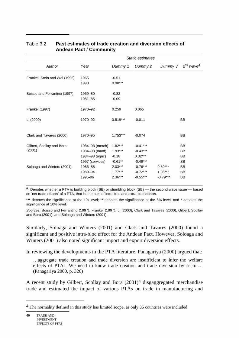
40 TRADE ANDINVESTMENTEFFECTS OF PTAS
Table 3.2 Past estimates of trade creation and diversion effects ofAndean Pact / Community
Static estimates
Author Year Dummy 1 Dummy 2 Dummy 3 2nd wavea
Frankel, Stein and Wei (1995) 19651990
-0.510.90***
Boisso and Ferrantino (1997) 1969–80
1981–85
-0.82
-0.09
Frankel (1997) 1970–92 0.259 0.065
Li (2000) 1970–92 0.819*** -0.011 BB
Clark and Tavares (2000) 1970–95 1.753*** -0.074 BB
Gilbert, Scollay and Bora(2001)
1984–98 (merch)1984–98 (manf)1984–98 (agric)
1997 (services)
1.82***1.93***-0.18
-0.61**
-0.41***-0.43***0.32***
-0.49***
BBBBBB
SBSoloaga and Winters (2001) 1986–88
1989–94
1995-96
2.03***1.77***
2.36***
-0.76***-0.72***
-0.55***
0.80***1.08***
-0.79***
BBBB
BB
a Denotes whether a PTA is building block (BB) or stumbling block (SB) — the second wave issue — basedon ‘net trade effects’ of a PTA, that is, the sum of intra-bloc and extra-bloc effects.
*** denotes the significance at the 1% level; ** denotes the significance at the 5% level; and * denotes thesignificance at 10% level.
Sources: Boisso and Ferrantino (1997), Frankel (1997), Li (2000), Clark and Tavares (2000), Gilbert, Scollayand Bora (2001), and Soloaga and Winters (2001).
Similarly, Soloaga and Winters (2001) and Clark and Tavares (2000) found asignificant and positive intra-bloc effect for the Andean Pact. However, Soloaga andWinters (2001) also noted significant import and export diversion effects.
In reviewing the developments in the PTA literature, Panagariya (2000) argued that:
…aggregate trade creation and trade diversion are insufficient to infer the welfareeffects of PTAs. We need to know trade creation and trade diversion by sector…(Panagariya 2000, p. 326)
A recent study by Gilbert, Scollay and Bora (2001)4 disgaggregated merchandisetrade and estimated the impact of various PTAs on trade in manufacturing and
4 The normality defined in this study has limited scope, as only 35 countries were included.
REVIEW OF THEEXISTING EMPIRICALEVIDENCE
41
agricultural products, separately. They also estimated creation and diversion effectsof trade in services. They found a positive intra-bloc effect and a negative extra-bloc effect for manufactured products, suggesting that though the overall bloc effectof Andean Pact/Community was positive, it had significantly diverted trade inmanufactured products from non-member countries. However, it had createdadditional trade in agricultural products with non-member countries. The estimateswere significant and negative for services, suggesting that trade in services wasbelow the expected levels for member and non-member countries of the AndeanPact/Community.
These various estimates reflect the changes made to the Andean Pact since itsinception. The pact was signed in 1969 and changed to the Andean Community in1996. It has included Bolivia, Colombia, Ecuador, Chile (left in 1976), Peru (left in1992) and Venezuela (joined in 1973). Initially, the agreement was ineffective. Allmembers, except Colombia, maintained significant barriers and there wereproduction-sharing arrangements between the countries during the first phase of itsoperation.
The agreement was revised in the mid 1980s in an effort to link individual countryreforms into a closer economic integration among the member countries. The resultwas free trade in some sectors, less bureaucracy, and an approach that was half freetrade area and half customs union. Trade among the members has grownconsiderably as the countries have liberalised their trade regimes and the AndeanCommunity has been reformed. However, trade is free from tariffs among only fourof the five member countries (Peru apart). Three countries share a common externaltariff, although there are exceptions even among these three. Meanwhile, Boliviaand Peru are outside the common external tariff.
Despite all this, the Andean Community seems to be moving forward with itsintegration goals, under the influence of a prospective Free Trade Area of theAmericas, and is expanding trade relations with other countries. These latterchanges were found effective, as suggested by the later gravity model estimatesreported in table 3.2.
This was a typical south-south agreement, with initial tariffs being reasonably high.Therefore, significant preferential trade liberalisation among members can beexpected to have increased intra-bloc trade significantly. Until recently, membercountries focused on border barriers related to merchandise trade. However,negotiations within the Andean Community have started on the harmonisation ofmacroeconomic and agricultural policies, and to develop and establish free trade inservices.
42 TRADE ANDINVESTMENTEFFECTS OF PTAS
The last column of table 3.2 reports the estimated ‘net trade effects’ of the AndeanPact/Community to assess the second wave issue. These results will be discussed indetail in section 3.3.
LAFTA/LAIA
Studies that have estimated the trade effects of LAFTA/LAIA are reported in table3.3. Boisso and Ferrantino (1997) included a number of bilateral trade determinantsand found that the intra-bloc effect of LAFTA/LAIA was negative in the initialyears, although it was positive and significant in later years. Other studies (Fink andPrimo Braga 1999, Li 2000 and Soloaga and Winters 2001) found a significant andpositive intra-bloc trade effect for members of LAFTA/LAIA. The study of Soloagaand Winters (2001) found that the LAIA produced significant import diversion, andexport diversion particularly in the early 1990s.
LAFTA was established early in the 1960s, and it eventually embraced all the SouthAmerican countries plus Mexico. In the LAFTA, high barriers to external tradewere maintained despite the Kennedy and Tokyo Rounds of multilateralliberalisation. Incoming investment was licensed. Within LAFTA, the reduction oftariffs and other barriers were negotiated based on product lists, which limited theextent of cross sector trade-offs. Other issues were likewise addressed in apiecemeal manner rather than on a comprehensive basis. Countries were initiallyenthusiastic about exchanging preferences within LAFTA, but once all the easyitems were liberalized, the process stalled when difficult sectors — autos, otherconsumer durables, agriculture, and textiles — came up for discussion. By 1980, theless ambitious Latin American Integration Association (LAIA) had replacedLAFTA. The LAIA was largely structured around bilateral trade preferences of themembers and a framework agreement for members of Andean and MERCOSUR.These changes have been partly reflected in the gravity model estimates, with theintra-bloc effect becoming positive, but the extra-bloc effect being increasinglynegative in the latter years.
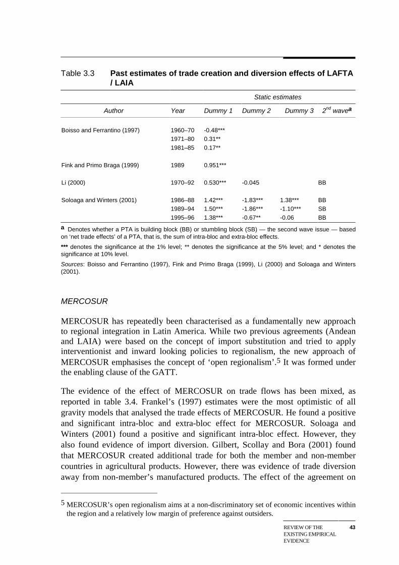
REVIEW OF THEEXISTING EMPIRICALEVIDENCE
43
Table 3.3 Past estimates of trade creation and diversion effects of LAFTA/ LAIA
Static estimates
Author Year Dummy 1 Dummy 2 Dummy 3 2nd wavea
Boisso and Ferrantino (1997) 1960–701971–80
1981–85
-0.48***0.31**
0.17**
Fink and Primo Braga (1999) 1989 0.951***
Li (2000) 1970–92 0.530*** -0.045 BB
Soloaga and Winters (2001) 1986–881989–94
1995–96
1.42***1.50***
1.38***
-1.83***-1.86***
-0.67**
1.38***-1.10***
-0.06
BBSB
BB
a Denotes whether a PTA is building block (BB) or stumbling block (SB) — the second wave issue — basedon ‘net trade effects’ of a PTA, that is, the sum of intra-bloc and extra-bloc effects.
*** denotes the significance at the 1% level; ** denotes the significance at the 5% level; and * denotes thesignificance at 10% level.
Sources: Boisso and Ferrantino (1997), Fink and Primo Braga (1999), Li (2000) and Soloaga and Winters(2001).
MERCOSUR
MERCOSUR has repeatedly been characterised as a fundamentally new approachto regional integration in Latin America. While two previous agreements (Andeanand LAIA) were based on the concept of import substitution and tried to applyinterventionist and inward looking policies to regionalism, the new approach ofMERCOSUR emphasises the concept of ‘open regionalism’.5 It was formed underthe enabling clause of the GATT.
The evidence of the effect of MERCOSUR on trade flows has been mixed, asreported in table 3.4. Frankel’s (1997) estimates were the most optimistic of allgravity models that analysed the trade effects of MERCOSUR. He found a positiveand significant intra-bloc and extra-bloc effect for MERCOSUR. Soloaga andWinters (2001) found a positive and significant intra-bloc effect. However, theyalso found evidence of import diversion. Gilbert, Scollay and Bora (2001) foundthat MERCOSUR created additional trade for both the member and non-membercountries in agricultural products. However, there was evidence of trade diversionaway from non-member’s manufactured products. The effect of the agreement on
5 MERCOSUR’s open regionalism aims at a non-discriminatory set of economic incentives within
the region and a relatively low margin of preference against outsiders.
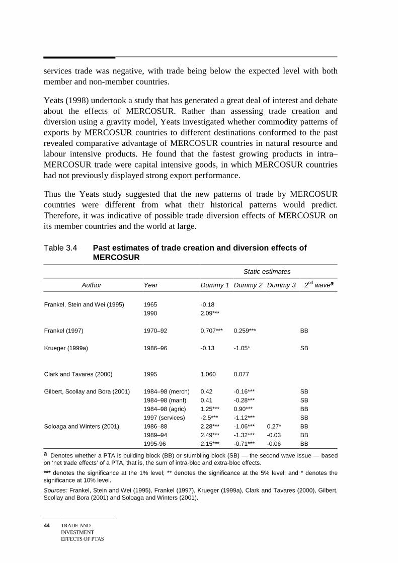
44 TRADE ANDINVESTMENTEFFECTS OF PTAS
services trade was negative, with trade being below the expected level with bothmember and non-member countries.
Yeats (1998) undertook a study that has generated a great deal of interest and debateabout the effects of MERCOSUR. Rather than assessing trade creation anddiversion using a gravity model, Yeats investigated whether commodity patterns ofexports by MERCOSUR countries to different destinations conformed to the pastrevealed comparative advantage of MERCOSUR countries in natural resource andlabour intensive products. He found that the fastest growing products in intra–MERCOSUR trade were capital intensive goods, in which MERCOSUR countrieshad not previously displayed strong export performance.
Thus the Yeats study suggested that the new patterns of trade by MERCOSURcountries were different from what their historical patterns would predict.Therefore, it was indicative of possible trade diversion effects of MERCOSUR onits member countries and the world at large.
Table 3.4 Past estimates of trade creation and diversion effects ofMERCOSUR
Static estimates
Author Year Dummy 1 Dummy 2 Dummy 3 2nd wavea
Frankel, Stein and Wei (1995) 19651990
-0.182.09***
Frankel (1997) 1970–92 0.707*** 0.259*** BB
Krueger (1999a) 1986–96 -0.13 -1.05* SB
Clark and Tavares (2000) 1995 1.060 0.077
Gilbert, Scollay and Bora (2001) 1984–98 (merch)
1984–98 (manf)1984–98 (agric)1997 (services)
0.42
0.411.25***-2.5***
-0.16***
-0.28***0.90***-1.12***
SB
SBBBSB
Soloaga and Winters (2001) 1986–881989–941995-96
2.28***2.49***2.15***
-1.06***-1.32***-0.71***
0.27*-0.03-0.06
BBBBBB
a Denotes whether a PTA is building block (BB) or stumbling block (SB) — the second wave issue — basedon ‘net trade effects’ of a PTA, that is, the sum of intra-bloc and extra-bloc effects.
*** denotes the significance at the 1% level; ** denotes the significance at the 5% level; and * denotes thesignificance at 10% level.
Sources: Frankel, Stein and Wei (1995), Frankel (1997), Krueger (1999a), Clark and Tavares (2000), Gilbert,Scollay and Bora (2001) and Soloaga and Winters (2001).
REVIEW OF THEEXISTING EMPIRICALEVIDENCE
45
However, Yeats study did not consider the imports into MERCOSUR countries,particularly from non-members, nor the trade and investment linkages amongmembers of MERCOSUR and with its non-members. Nagarajan (1998) arguedinstead that intra-regional trade should be compared with extra-regional imports, notextra-regional exports, and that by focusing on the latter, Yeats may haveexaggerated the effects of MERCOSUR.
Chang and Winters (2000) conducted a study that assessed the welfare effects ofMERCOSUR by looking at changes in import and export prices of commoditiestraded between Brazil, Argentina and the rest of the world. They assumed that non-member countries exported to two segmented markets, Brazil and the rest of theworld. In an imperfectly competitive setting with differentiated products, thechanges in Brazil’s general tariff rates led to price changes by non-member firmsexporting to Brazil, and tariff preferences offered to member Argentina led toadditional strategic price responses within the Brazilian market. They identifiedboth such responses in commodity-level import data from Brazil and export datafrom Brazil’s major trading partners — including United States, Germany, Italy,and Japan. They found that general tariff changes and preferential tariffs bothaffected Brazil’s import prices significantly, and that MERCOSUR’s preferentialtariffs caused a significant decline, ceteris paribus, in the prices of non-members’exports to Brazil. They concluded that:
Even if a PTA aims only to facilitate trade between the constituent territories and not toraise barriers to the trade of other contracting parties with such territories and indeed,even if, as with MERCOSUR, it simultaneously undertakes a general tradeliberalisation, other contracting parties may still be affected adversely, because they arecompelled to reduce their prices to meet competition from suppliers within the PTA …Of course this is only one part of the overall welfare calculus for non-members. Oneneeds also to consider the prices of their imports from the bloc and any volume effectson trade, which could tip the balance and generate overall gains. Nonetheless, theeffects identified here are large enough to warrant serious consideration. (Chang andWinters 2000, p. 32-3)
Based on casual evidence, MERCOSUR appears successful at stimulating trade andinvestment. Intra-MERCOSUR exports grew by an average of 30 per cent a year inits first five years of existence. MERCOSUR has not visibly restricted its trade andinvestment with the rest of the world, and both EU and US exports to thesecountries have grown at reasonable rates (WTF 2000, UNCTAD 1994).6
Like the original EC, MERCOSUR served an important political purpose, namelydefusing tensions between Argentina and Brazil. Unlike earlier Latin American 6 Exports from the United States to MERCOSUR grew at 1.1 per cent a year between 1991 and
1997. Exports from the EU to MERCOSUR grew at 6.7 per cent a year over the same period, orat 2.8 per cent a year if exports from Austria, Finland and Sweden are excluded.
46 TRADE ANDINVESTMENTEFFECTS OF PTAS
regional agreements, the MERCOSUR countries reduced their external barriers,liberalised investment, and tackled a range of sectors.7
However, many challenges remain to be tackled within MERCOSUR. Brazil named200 tariff lines in the exceptions list, mainly sensitive industries such as computers,electronics, chemical, agriculture, textiles, capital goods and the automotiveindustry. A combination of unilateral liberalisation and MERCOSUR negotiatedchanges reduced members tariffs substantially from an average of 50 per cent in1988 to a common external tariff average of 12 per cent in 1995. However, it hasremained the case that trade policy in Brazil has been subject to frequent changes tomeet short-term political objectives. For example, tariffs on textiles, toys and motorvehicles were increased to 70 per cent for non-members in 1995. Although it is tooearly for these later changes to be reflected in gravity model estimates, nonethelessthey raise a serious concern for the welfare of both members and non-members ofthis agreement. Preusse (2001) reviewed the progress of the MERCOSURagreement and argued that during 1991–1995, the integration process wassuccessful, but that after 1995, the integration process had virtually come to astandstill because of the inconsistency of the ‘open regionalism’ concept with theescape strategy on key sensitive sectors.
NAFTA
In table 3.5, the coefficient for the intra-bloc trade effect of NAFTA was found tobe positive and significant only in Frankel’s (1997) study. Gilbert, Scollay and Bora(2001) found a significant but negative NAFTA effect on its members’manufacturing trade. All other studies (Krueger 1999a, Clark and Tavares 2000,Soloaga and Winters 2001) found an insignificant effect for NAFTA on members’trade flows. There was clear evidence that NAFTA diverted trade from non-members, as indicated by the negative sign on the second and third dummycoefficients.
7 The auto industry is an important growth industry in MERCOSUR. Since Brazil had been a low
cost producer, it was economically efficient for foreign firms to establish their plants in Brazil inorder to serve a large MERCOSUR market. Argentina was worried that low cost Brazil wouldattract all of the foreign investment and dominate the market. Therefore, it was necessary toensure that some of the foreign investment was directed to Argentina in the absence of a directcompensation mechanism in the agreement. To convince Argentina to agree to the PTA, the autosectoral agreement was enacted. It is called the Compensated Trade Clause, which requires eachfirm to balance its trade between Brazil and Argentina. This mitigates the diversion problem byforcing firms to produce some models in Argentina and it enticed the governments to sign thePTA.
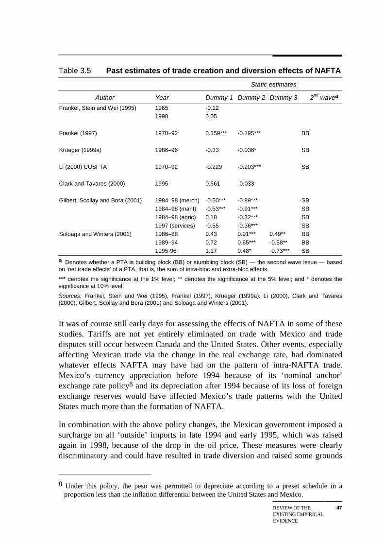
REVIEW OF THEEXISTING EMPIRICALEVIDENCE
47
Table 3.5 Past estimates of trade creation and diversion effects of NAFTA
Static estimates
Author Year Dummy 1 Dummy 2 Dummy 3 2nd wavea
Frankel, Stein and Wei (1995) 19651990
-0.120.05
Frankel (1997) 1970–92 0.359*** -0.195*** BB
Krueger (1999a) 1986–96 -0.33 -0.036* SB
Li (2000) CUSFTA 1970–92 -0.229 -0.203*** SB
Clark and Tavares (2000) 1995 0.561 -0.033
Gilbert, Scollay and Bora (2001) 1984–98 (merch)1984–98 (manf)
1984–98 (agric)1997 (services)
-0.50***-0.53***
0.18-0.55
-0.89***-0.91***
-0.32***-0.36***
SBSB
SBSB
Soloaga and Winters (2001) 1986–88
1989–941995-96
0.43
0.721.17
0.91***
0.65***0.48*
0.49**
-0.58**-0.73***
BB
BBSB
a Denotes whether a PTA is building block (BB) or stumbling block (SB) — the second wave issue — basedon ‘net trade effects’ of a PTA, that is, the sum of intra-bloc and extra-bloc effects.
*** denotes the significance at the 1% level; ** denotes the significance at the 5% level; and * denotes thesignificance at 10% level.
Sources: Frankel, Stein and Wei (1995), Frankel (1997), Krueger (1999a), Li (2000), Clark and Tavares(2000), Gilbert, Scollay and Bora (2001) and Soloaga and Winters (2001).
It was of course still early days for assessing the effects of NAFTA in some of thesestudies. Tariffs are not yet entirely eliminated on trade with Mexico and tradedisputes still occur between Canada and the United States. Other events, especiallyaffecting Mexican trade via the change in the real exchange rate, had dominatedwhatever effects NAFTA may have had on the pattern of intra-NAFTA trade.Mexico’s currency appreciation before 1994 because of its ‘nominal anchor’exchange rate policy8 and its depreciation after 1994 because of its loss of foreignexchange reserves would have affected Mexico’s trade patterns with the UnitedStates much more than the formation of NAFTA.
In combination with the above policy changes, the Mexican government imposed asurcharge on all ‘outside’ imports in late 1994 and early 1995, which was raisedagain in 1998, because of the drop in the oil price. These measures were clearlydiscriminatory and could have resulted in trade diversion and raised some grounds
8 Under this policy, the peso was permitted to depreciate according to a preset schedule in a
proportion less than the inflation differential between the United States and Mexico.
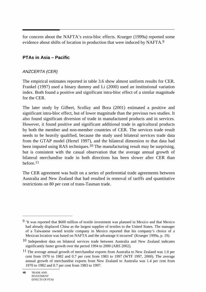
48 TRADE ANDINVESTMENTEFFECTS OF PTAS
for concern about the NAFTA’s extra-bloc effects. Krueger (1999a) reported someevidence about shifts of location in production that were induced by NAFTA.9
PTAs in Asia – Pacific
ANZCERTA (CER)
The empirical estimates reported in table 3.6 show almost uniform results for CER.Frankel (1997) used a binary dummy and Li (2000) used an institutional variationindex. Both found a positive and significant intra-bloc effect of a similar magnitudefor the CER.
The later study by Gilbert, Scollay and Bora (2001) estimated a positive andsignificant intra-bloc effect, but of lower magnitude than the previous two studies. Italso found significant diversion of trade in manufactured products and in services.However, it found positive and significant additional trade in agricultural productsby both the member and non-member countries of CER. The services trade resultneeds to be heavily qualified, because the study used bilateral services trade datafrom the GTAP model (Hertel 1997), and the bilateral dimension to that data hadbeen imputed using RAS techniques.10 The manufacturing result may be surprising,but is consistent with the casual observation that the average annual growth ofbilateral merchandise trade in both directions has been slower after CER thanbefore.11
The CER agreement was built on a series of preferential trade agreements betweenAustralia and New Zealand that had resulted in removal of tariffs and quantitativerestrictions on 80 per cent of trans-Tasman trade.
9 ‘It was reported that $600 million of textile investment was planned in Mexico and that Mexico
had already displaced China as the largest supplier of textiles to the United States. The managerof a Taiwanese owned textile company in Mexico reported that his company’s choice of aMexican location was based on NAFTA and the advantage it incurred’ (Krueger 1999a, p. 19).
10 Independent data on bilateral services trade between Australia and New Zealand indicatessignificantly faster growth over the period 1994 to 2000 (ABS 2002).
11 The average annual growth of merchandise exports from Australia to New Zealand was 1.0 percent from 1970 to 1982 and 0.7 per cent from 1983 to 1997 (WTF 1997, 2000). The averageannual growth of merchandise exports from New Zealand to Australia was 1.4 per cent from1970 to 1982 and 0.7 per cent from 1983 to 1997.
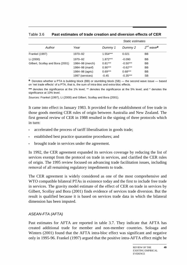
REVIEW OF THEEXISTING EMPIRICALEVIDENCE
49
Table 3.6 Past estimates of trade creation and diversion effects of CER
Static estimates
Author Year Dummy 1 Dummy 2 2nd wavea
Frankel (1997) 1970–92 1.554*** 0.021 BB
Li (2000) 1970–92 1.872*** -0.090 BBGilbert, Scollay and Bora (2001) 1984–98 (merch)
1984–98 (manf)
1984–98 (agric)1997 (services)
0.81***0.90***
0.69***-0.45
-0.50***-0.62***
0.68***-0.35***
BBBB
BBSB
a Denotes whether a PTA is building block (BB) or stumbling block (SB) — the second wave issue — basedon ‘net trade effects’ of a PTA, that is, the sum of intra-bloc and extra-bloc effects.
*** denotes the significance at the 1% level; ** denotes the significance at the 5% level; and * denotes thesignificance at 10% level.
Sources: Frankel (1997), Li (2000) and Gilbert, Scollay and Bora (2001).
It came into effect in January 1983. It provided for the establishment of free trade inthose goods meeting CER rules of origin between Australia and New Zealand. Thefirst general review of CER in 1988 resulted in the signing of three protocols whichin turn:
• accelerated the process of tariff liberalisation in goods trade;
• established best practice quarantine procedures; and
• brought trade in services under the agreement.
In 1992, the CER agreement expanded its services coverage by reducing the list ofservices exempt from the protocol on trade in services, and clarified the CER rulesof origin. The 1995 review focused on advancing trade facilitation issues, includingremoval of all remaining regulatory impediments to trade.
The CER agreement is widely considered as one of the most comprehensive andWTO compatible bilateral PTAs in existence today and the first to include free tradein services. The gravity model estimate of the effect of CER on trade in services byGilbert, Scollay and Bora (2001) finds evidence of services trade diversion. But theresult is qualified because it is based on services trade data in which the bilateraldimension has been imputed.
ASEAN-FTA (AFTA)
Past estimates for AFTA are reported in table 3.7. They indicate that AFTA hascreated additional trade for member and non-member countries. Soloaga andWinters (2001) found that the AFTA intra-bloc effect was significant and negativeonly in 1995-96. Frankel (1997) argued that the positive intra-AFTA effect might be
50 TRADE ANDINVESTMENTEFFECTS OF PTAS
partly due to Singapore’s entrepot trade. To examine this, he included a Singapore-specific dummy variable in the gravity model and found that
The Singapore dummy does indeed have a positive and very significant coefficient(1.51). The coefficient on the ASEAN dummy is reduced to 1.40 but remainsquantitatively large and statistically significant. This suggests that Singapore’s extremeopenness does not explain all of the apparent inward bias among the ASEAN countries(Frankel 1997, p. 98)
The ASEAN countries negotiated a PTA in 1977, but it had a limitedimplementation, because of administrative protection and opposition by industrialand agricultural interests.
In 1989, the fraction of goods eligible for preferences was only 3 per cent (Frankel1997). It was not until 1992 that that ASEAN Free Trade Area (AFTA) was formed,which would be implemented by reducing tariffs and non-tariff barriers in phasesfrom 1993 to 2008. AFTA was formed under the Enabling Clause of the GATT (seeBox 1.1).
Table 3.7 Past estimates of trade creation and diversion effects ofASEAN–FTA
Static estimates
Author Year Dummy 1 Dummy 2 Dummy 3 2nd wavea
Frankel (1997) 1970–92 1.318*** 0.767*** BB
Fink and Primo Braga (1999) 1989 2.476***
Krueger (1999a) 1986–96 0.78* 0.16* BB
Li (2000) 1970–92 1.311*** 0.653*** BB
Clark and Tavares (2000) 1995 1.673* 0.489* BB
Gilbert, Scollay and Bora(2001)
1984–98 (merch)
1984–98 (manf)1984–98 (agric)1997 (services)
0.65***
0.63***0.32***1.08***
0.54***
0.54***0.45***1.01***
BB
BBBBBB
Soloaga and Winters (1999) 1986–881989–941995-96
0.180.09-1.06***
0.150.30**0.82***
0.70***0.67***0.99***
BBBBBB
a Denotes whether a PTA is building block (BB) or stumbling block (SB) — the second wave issue — basedon ‘net trade effects’ of a PTA, that is, the sum of intra-bloc and extra-bloc effects.
*** denotes the significance at the 1% level; ** denotes the significance at the 5% level; and * denotes thesignificance at 10% level.
Sources: Frankel, Stein and Wei (1995), Frankel (1997), Krueger (1999a), Li (2000), Clark and Tavares(2000), Gilbert, Scollay and Bora (2001), Soloaga and Winters (1999).
REVIEW OF THEEXISTING EMPIRICALEVIDENCE
51
AFTA is politically and economically a diverse group and intra-AFTA tradeaccounted for only 15 per cent of AFTA exports in 1997, about half of which wasentrepot trade with Singapore that was basically duty-free already. AFTA membersvary greatly in the composition of their exports (industrial and agricultural) andtheir levels of protection. Consequently, going to zero tariffs on substantially allgoods will entail a very asymmetric impact on AFTA countries.
Singapore and Malaysia have significantly increased their bilateral trade with allother AFTA and non-AFTA members between 1986 and 1998. These two arerelatively high-income countries and relatively open, compared with other AFTAmembers. Theory suggests that such economies would receive only limited benefitfrom the formation of a PTA under the assumption of constant production costs. Butwith less-than-perfect competition, both countries might have benefited from thediversion of trade by other AFTA countries (De Rosa 1998). These two countriessupply the largest proportion of the increased intra-regional demand formanufactures previously supplied by non-members of AFTA. Besides, Singaporemight have also benefited from its real exchange rate appreciation with the othermembers of AFTA. This could be the possible reason for the positive and consistentintra- and extra-AFTA effects found by previous studies.
PTAs in Europe
EC/EU
Of all the PTAs, EC/EU is the one with the most far-reaching implications. It is themost long-lived and it:
• started life as a customs union;
• created a regional mechanism for limiting exchange rate flexibility amongmembers in the 1970s;
• established an integrated internal market in which goods, services, capital andlabour could flow in the 1990s;
• expanded its membership four times and plans to integrate eastern Europeancountries; and
• started monetary integration of members in 1995 and the currency union cameinto existence in January 2002.
Reflecting these changes, the empirical estimates reported in table 3.8 for EC/EUare not consistent across the studies.
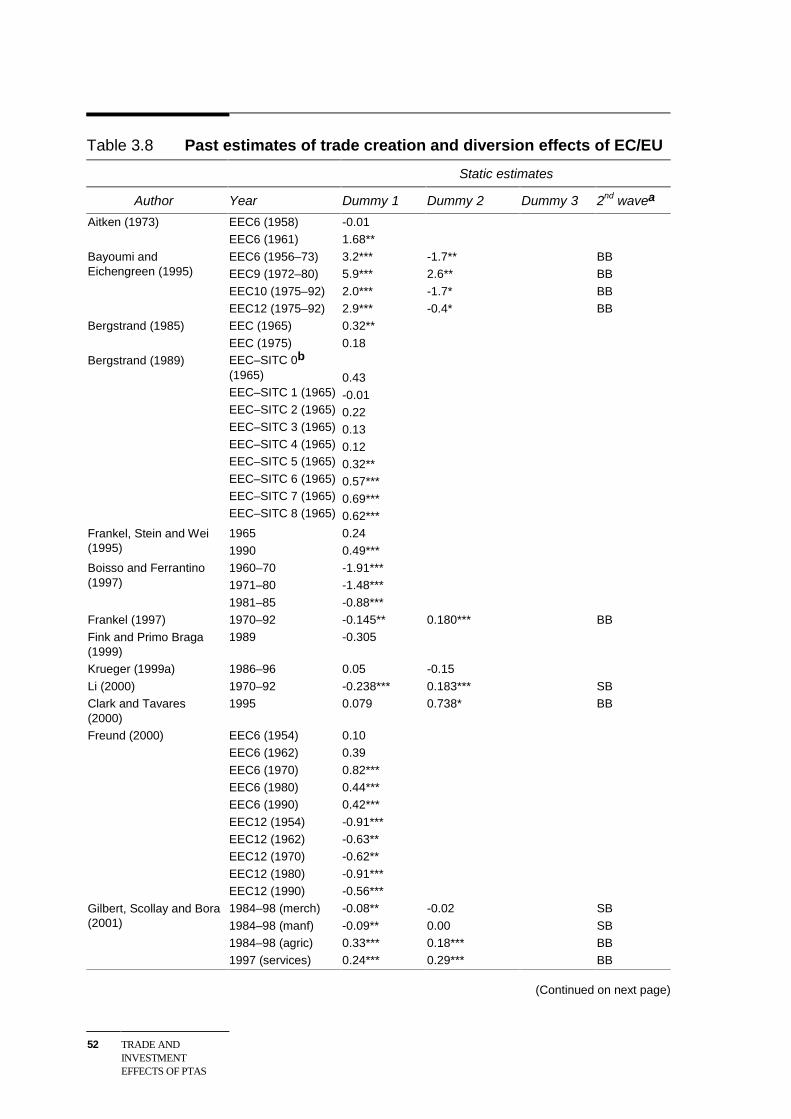
52 TRADE ANDINVESTMENTEFFECTS OF PTAS
Table 3.8 Past estimates of trade creation and diversion effects of EC/EU
Static estimates
Author Year Dummy 1 Dummy 2 Dummy 3 2nd wavea
Aitken (1973) EEC6 (1958)EEC6 (1961)
-0.011.68**
Bayoumi andEichengreen (1995)
EEC6 (1956–73)EEC9 (1972–80)
EEC10 (1975–92)EEC12 (1975–92)
3.2***5.9***
2.0***2.9***
-1.7**2.6**
-1.7*-0.4*
BBBB
BBBB
Bergstrand (1985) EEC (1965)
EEC (1975)
0.32**
0.18Bergstrand (1989) EEC–SITC 0b
(1965)EEC–SITC 1 (1965)EEC–SITC 2 (1965)
EEC–SITC 3 (1965)EEC–SITC 4 (1965)EEC–SITC 5 (1965)
EEC–SITC 6 (1965)EEC–SITC 7 (1965)EEC–SITC 8 (1965)
0.43
-0.010.220.13
0.120.32**0.57***
0.69***0.62***
Frankel, Stein and Wei(1995)
1965
1990
0.24
0.49***Boisso and Ferrantino(1997)
1960–701971–80
1981–85
-1.91***-1.48***
-0.88***Frankel (1997) 1970–92 -0.145** 0.180*** BB
Fink and Primo Braga(1999)
1989 -0.305
Krueger (1999a) 1986–96 0.05 -0.15
Li (2000) 1970–92 -0.238*** 0.183*** SBClark and Tavares(2000)
1995 0.079 0.738* BB
Freund (2000) EEC6 (1954)EEC6 (1962)
EEC6 (1970)EEC6 (1980)EEC6 (1990)
EEC12 (1954)EEC12 (1962)EEC12 (1970)
EEC12 (1980)EEC12 (1990)
0.100.39
0.82***0.44***0.42***
-0.91***-0.63**-0.62**
-0.91***-0.56***
Gilbert, Scollay and Bora(2001)
1984–98 (merch)
1984–98 (manf)1984–98 (agric)1997 (services)
-0.08**
-0.09**0.33***0.24***
-0.02
0.000.18***0.29***
SB
SBBBBB
(Continued on next page)

REVIEW OF THEEXISTING EMPIRICALEVIDENCE
53
Table 3.8 (Continued) Static estimates
Author Year Dummy 1 Dummy 2 Dummy 3 2nd wavea
Soloaga and Winters(2001)
1986–88
1989–941995–96
-1.45***
-1.17***-0.88***
1.25***
0.89***0.72***
0.49***
0.07-0.15*
BB
SBSB
a Denotes whether a PTA is building block (BB) or stumbling block (SB) — the second wave issue —based on‘net trade effects’ of a PTA, that is, the sum of intra-bloc and extra-bloc effects. b SITC 0 denotes food andlive animals; SITC 1 denotes beverages and tobacco; SITC 2 denotes raw materials; SITC 3 denotes fuels;SITC 4 denotes animal and vegetable oils and fats; SITC 5 denotes chemicals; SITC 6 denotes manufactureschiefly by material; SITC 7 denotes machinery and transport euipment; and SITC 8 denotes miscellaneousmanufactures.
*** denotes the significance at the 1% level; ** denotes the significance at the 5% level; and * denotes thesignificance at 10% level.
Sources: Aitken (1973), Bergstrand (1985, 1989), Bayoumi and Eichengreen (1995), Frankel, Stein and Wei(1995), Boisso and Ferrantino (1997), Frankel (1997), Fink and Primo Braga (1999), Krueger (1999a), Li(2000), Clark and Tavares (2000), Freund (2000), Gilbert, Scollay and Bora (2001) and Soloaga and Winters(2001).
The initial study by Aitken (1973) found that the EC experienced more growth intrade during the post-integration period than during pre-integration period. Heapplied only an intra-bloc dummy to assess EC’s impact collectively on the bloc —a gross trade creation effect. According to his estimates, by 1961, intra-EC tradewas ceteris paribus, 1.68 times larger than ‘normal’ European trade.
Bergstrand’s (1985, 1989) focus was on investigating the microeconomicfoundations behind the gravity model and related bilateral trade determinants. Heincluded the exchange rate and unit export and import price indices in his 1985gravity model and found that the EC’s intra-bloc effect in 1965 was positive andsignificant, but it turned out to be insignificant by the year 1975. In his later study,in addition to the above variables, he included per capita income as a proxy forfactor endowments. He disaggregated the merchandise trade into SITC one digitindustries and found that the intra-bloc effect for high SITC code manufacturedproducts (generally more highly processed) was more positive and significant thanfor lower SITC categories (including agriculture) in 1965.
Bayoumi and Eichengreen (1995) found that the creation and expansion of the ECwas responsible for increased trade volumes. For the founding members of EC6, thetrade creating effects were greater in the early years, consistent with the previousgravity model estimates for the same period by Aitken (1973) and Bergstrand(1985, 1989). One concern raised in the literature at that time was the impact ofunobserved variables biasing the PTA dummy coefficient. Bayoumi andEichengreen (1995) addressed this issue by simply differencing the variables. Theyargued that:
54 TRADE ANDINVESTMENTEFFECTS OF PTAS
We estimate our equation in differences rather than levels; thus unobservedheterogeneity across countries that is constant over time will not contaminate ourresults. (Bayoumi and Eichengreen 1995, p. ii)
The above four studies used data on trade among European countries excludingtrade among most non-European countries. So their standard of comparison hadlimited scope. These studies also did not include a number of bilateral tradedeterminants. Therefore, it is possible that the PTA dummies would have picked upsome of their effects. After controlling for common language and a common border,Frankel, Stein and Wei (1995) found an insignificant intra-bloc effect for the EC in1965, in contrast to the Bergstrand (1985) result for the same year.
Later studies reported in table 3.8 found that intra-bloc trade can be mostlyexplained by the various bilateral trade determinants. Boisso and Ferrantino (1997)found that trade among EC members was significantly less than would be predictedby the normal bilateral trade determinants. The negative effect steadily erodedthrough to the mid-1980s. Similar results for the intra-bloc effects of EC/EU wereobtained by Frankel (1997), Fink and Primo Braga (1999) and Li (2000). Fordisaggregated trade, Gilbert, Scollay and Bora (2001) found that the intra-bloceffect of EC/EU was positive and significant for agricultural products (despite EUagricultural measures being primarily about domestic support, not trade) andservices, but not for manufactured products.
The effect of EC/EU on non-member countries was mixed. Bayoumi andEichengreen (1995) found that each expansion of the EC had a different effect onnon-member countries. The first expansion in 1973, which added Denmark, Irelandand United Kingdom, created additional trade for members and non-members. Thesubsequent expansions, including Greece in 1981 and Spain and Portugal in 1986,created additional trade for members and diverted trade from non-membercountries. Frankel (1997) found a positive intra-bloc and negative extra-bloc effectfor the EU. He regarded this evidence in a very positive light:
…[the] net political effect of the removal of regional barriers can be to supportliberalization with respect to non-members as well. The effect of further liberalizationhas in many cases been more than enough to offset any trade diversion resultingdirectly from the original arrangements themselves. (Frankel 1997, p. 227)
Frankel’s conclusion appears to be optimistic. In a later study, Soloaga and Winters(2001) found that the propensity to export and import from non-members of the EUfalls over time, suggesting trade diversion. They found
evidence of export diversion in EU and EFTA, which would be consistent with theirimposing a welfare cost on the [rest of the world]. (Soloaga and Winters 2001, p.)
REVIEW OF THEEXISTING EMPIRICALEVIDENCE
55
Freund (2000) argued that in the presence of sunk costs, the trade diversion effectsof PTAs could be permanent. She used the EC to test the evidence of first moveradvantages among its six founding members. Her hypothesis was that trade betweenthe original members would be larger than otherwise predicted by the gravitymodel, even after other countries had joined the union. Her gravity model resultswere consistent with her hypothesis that early entry into the union allowed countriesto establish trade links that persisted over time. The intra-bloc effect on earlymembers was positive and significant, while the intra-bloc effect on later memberswas significant but negative.
EFTA
Some studies that analysed the EC also analysed EFTA during the 1960s and 1970s,though EC is a customs union and EFTA is a free trade area. The gravity modelestimates were similar for both PTAs in the initial periods of their implementation.Aitken (1973) found a significant intra-bloc trade effect for EFTA, althoughsubstantially less in proportional terms than the effect for the EC.
Bayoumi and Eichengreen (1995) reached a similar conclusion that the trade effectswere concentrated in the earlier years of EFTA formation. However, they foundthat, for the later years, the intra-bloc trade effect was negative because of the lossof two key countries, the United Kingdom and Denmark, to the EC.
Studies by Frankel, Stein and Wei (1995), Boisso and Ferrantino (1997), and Finkand Primo Braga (1999) found an insignificant effect of EFTA on members’ tradeflows. These studies applied only an intra-bloc dummy to assess the PTAs.
Frankel (1997), Li (2000) and Clark and Tavares (2000) used both intra-bloc andextra-bloc dummy variables and found a positive and significant effect of EFTA onmembers’ trade. However, its effect on non-member countries was negative.Soloaga and Winters (2001) found similar results for EFTA as for EC/EU andconcluded that the propensity for EFTA members to export and import from non-members fell over time, suggesting trade diversion.
As noted, a major limitation of the gravity model studies reviewed here is that fewhave controlled for all of the bilateral trade determinants listed in table 3.1, and fewhave controlled for additional but unobservable country- or time-specific influenceson bilateral trade. As a result, the influence of the omitted variables could bewrongly attributed to the PTA dummy variables, although it is difficult to evaluateby how much.
In addition, the technique of making one or several cross-sectional estimates hasseveral drawbacks. It risks attributing trade effects to PTAs ‘before the event’, and
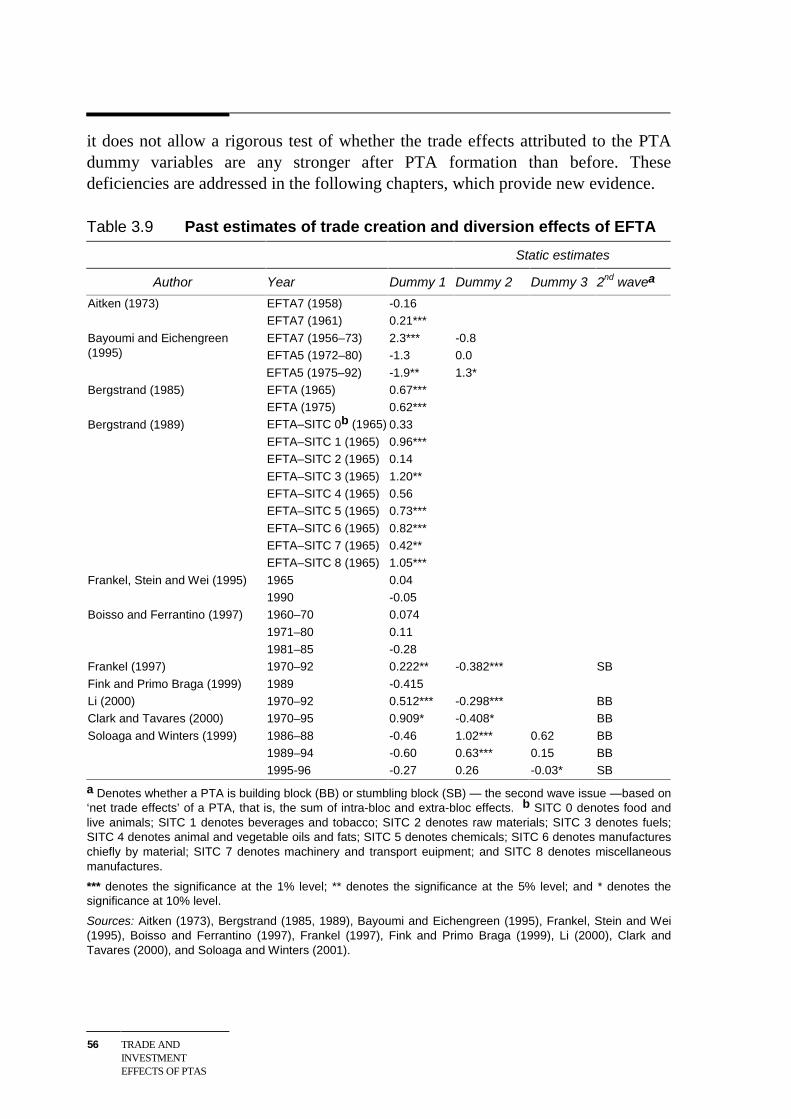
56 TRADE ANDINVESTMENTEFFECTS OF PTAS
it does not allow a rigorous test of whether the trade effects attributed to the PTAdummy variables are any stronger after PTA formation than before. Thesedeficiencies are addressed in the following chapters, which provide new evidence.
Table 3.9 Past estimates of trade creation and diversion effects of EFTA
Static estimates
Author Year Dummy 1 Dummy 2 Dummy 3 2nd wavea
Aitken (1973) EFTA7 (1958)EFTA7 (1961)
-0.160.21***
Bayoumi and Eichengreen(1995)
EFTA7 (1956–73)EFTA5 (1972–80)
EFTA5 (1975–92)
2.3***-1.3
-1.9**
-0.80.0
1.3*Bergstrand (1985) EFTA (1965)
EFTA (1975)0.67***0.62***
Bergstrand (1989) EFTA–SITC 0b (1965)
EFTA–SITC 1 (1965)EFTA–SITC 2 (1965)
EFTA–SITC 3 (1965)EFTA–SITC 4 (1965)EFTA–SITC 5 (1965)
EFTA–SITC 6 (1965)EFTA–SITC 7 (1965)EFTA–SITC 8 (1965)
0.330.96***0.14
1.20**0.560.73***
0.82***0.42**1.05***
Frankel, Stein and Wei (1995) 19651990
0.04-0.05
Boisso and Ferrantino (1997) 1960–70
1971–801981–85
0.074
0.11-0.28
Frankel (1997) 1970–92 0.222** -0.382*** SB
Fink and Primo Braga (1999) 1989 -0.415Li (2000) 1970–92 0.512*** -0.298*** BBClark and Tavares (2000) 1970–95 0.909* -0.408* BB
Soloaga and Winters (1999) 1986–881989–941995-96
-0.46-0.60-0.27
1.02***0.63***0.26
0.620.15-0.03*
BBBBSB
a Denotes whether a PTA is building block (BB) or stumbling block (SB) — the second wave issue —based on‘net trade effects’ of a PTA, that is, the sum of intra-bloc and extra-bloc effects. b SITC 0 denotes food andlive animals; SITC 1 denotes beverages and tobacco; SITC 2 denotes raw materials; SITC 3 denotes fuels;SITC 4 denotes animal and vegetable oils and fats; SITC 5 denotes chemicals; SITC 6 denotes manufactureschiefly by material; SITC 7 denotes machinery and transport euipment; and SITC 8 denotes miscellaneousmanufactures.
*** denotes the significance at the 1% level; ** denotes the significance at the 5% level; and * denotes thesignificance at 10% level.
Sources: Aitken (1973), Bergstrand (1985, 1989), Bayoumi and Eichengreen (1995), Frankel, Stein and Wei(1995), Boisso and Ferrantino (1997), Frankel (1997), Fink and Primo Braga (1999), Li (2000), Clark andTavares (2000), and Soloaga and Winters (2001).
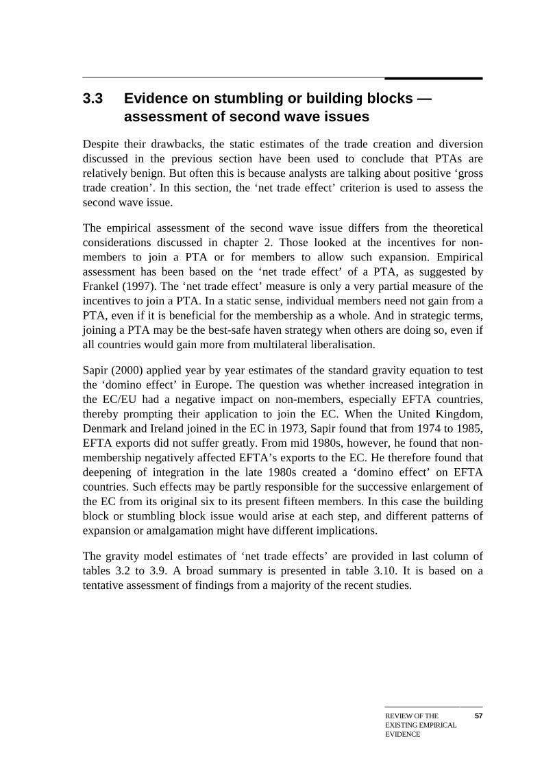
REVIEW OF THEEXISTING EMPIRICALEVIDENCE
57
3.3 Evidence on stumbling or building blocks —assessment of second wave issues
Despite their drawbacks, the static estimates of the trade creation and diversiondiscussed in the previous section have been used to conclude that PTAs arerelatively benign. But often this is because analysts are talking about positive ‘grosstrade creation’. In this section, the ‘net trade effect’ criterion is used to assess thesecond wave issue.
The empirical assessment of the second wave issue differs from the theoreticalconsiderations discussed in chapter 2. Those looked at the incentives for non-members to join a PTA or for members to allow such expansion. Empiricalassessment has been based on the ‘net trade effect’ of a PTA, as suggested byFrankel (1997). The ‘net trade effect’ measure is only a very partial measure of theincentives to join a PTA. In a static sense, individual members need not gain from aPTA, even if it is beneficial for the membership as a whole. And in strategic terms,joining a PTA may be the best-safe haven strategy when others are doing so, even ifall countries would gain more from multilateral liberalisation.
Sapir (2000) applied year by year estimates of the standard gravity equation to testthe ‘domino effect’ in Europe. The question was whether increased integration inthe EC/EU had a negative impact on non-members, especially EFTA countries,thereby prompting their application to join the EC. When the United Kingdom,Denmark and Ireland joined in the EC in 1973, Sapir found that from 1974 to 1985,EFTA exports did not suffer greatly. From mid 1980s, however, he found that non-membership negatively affected EFTA’s exports to the EC. He therefore found thatdeepening of integration in the late 1980s created a ‘domino effect’ on EFTAcountries. Such effects may be partly responsible for the successive enlargement ofthe EC from its original six to its present fifteen members. In this case the buildingblock or stumbling block issue would arise at each step, and different patterns ofexpansion or amalgamation might have different implications.
The gravity model estimates of ‘net trade effects’ are provided in last column oftables 3.2 to 3.9. A broad summary is presented in table 3.10. It is based on atentative assessment of findings from a majority of the recent studies.
58 TRADE ANDINVESTMENTEFFECTS OF PTAS
Table 3.10 Building blocks or stumbling blocks to free tradeBased on ‘net trade effect’ criterion
Building blocks Stumbling blocks Inconclusive
Andean CommunityCERAFTA
EEC/EU?EFTA?
NAFTA LAIAMERCOSUR
Sources: Tables 3.2 to 3.9.
Based on the past gravity model studies, Andean, CER, AFTA, and possiblyEEC/EU and EFTA have liberalised more internally than they have diverted tradefrom the rest of the world, as indicated by their positive ‘net trade effect’.Conversely, NAFTA has created negative net effects. The majority findings forLAIA and MERCOSUR are inconclusive.
For trade in agricultural products, based on the one available study, NAFTA wasassessed as net trade diverting (see table 3.5) and surprisingly, EU was found to benet trade creating (Gilbert, Scollay and Bora 2001). Agriculture is characterised bymassive intervention and numerous exceptions from general WTO rules. Thetreatment of agriculture in PTAs varies widely and in most cases, countriesparticipating in PTAs carefully craft their agreements so that they do not interferewith the autonomy of domestic farm programs and national food policies. In somecases, agriculture has been totally excluded because it was deemed too difficult tonegotiate.
EU has a number of bilateral agreements with the Eastern European andMediterranean countries and it has a generalised system of preferences (GSP) withmany developing countries. This could partly explain the positive and significanteffects of EU’s agricultural trade with the non-member countries. A number of EUbilateral agreements will be empirically assessed in chapter 4. In addition, EU’sexport subsidies may have enhanced trade in agricultural products with thedeveloping non-member countries. However, this does not take into account thedomestic inefficiencies caused by the Common Agricultural Policy (CAP).
For NAFTA, the agricultural provisions consist of three bilateral agreements. TheUnited States exports highly subsidised agricultural raw materials, particularlycotton and cereals, to Mexico. The rules of origin allow Mexico to re-export itsimports after processing. This could have created high trade diversion on theagricultural exports of non-member countries to the United States. The effects ofrules of origin on members’ and non-members’ trade flows are discussed further inchapter 4.
REVIEW OF THEEXISTING EMPIRICALEVIDENCE
59
The majority of studies find almost all PTAs to be net trade creating rather thandiverting — a relatively benign finding. Further, a comparison of gravity modelestimates of first and second wave issues can lead to different policy conclusions.For example, when Spain and Portugal joined the EC, it led to trade diversion fromnon-members (Bayoumi and Eichengreen 1995). But it could be considereddesirable on ‘dynamic path’ grounds because it signified expanding membershipand hence progress towards the goal of achieving multilateral trade liberalisation.
The net trade effect test is only a weak test of whether the gains from trade creationoutweigh the costs of trade diversion. It provides some positive evidence forcombined consumer and producer surplus (the triangles ABC and FGH in figure2.1), but it does not indicate whether their combined area exceeds that of lost tariffrevenue (the trapezoid BEJG in figure 2.1).
3.4 Evidence on investment creation and diversioneffects of PTAs — assessment of third wave issues
Empirical work on PTAs has mostly focused on static trade creation and tradediversion — the first wave issue.
However, countries participating in PTAs are equally concerned about the impacton investment flows and the potential for investment creation and diversion — athird wave issue. It was believed that the creation of NAFTA would attract foreigndirect investment (FDI) into Mexico. There was a surge in investment prior to theformation of NAFTA in the early 1990s. Spain and Portugal also experiencedsimilar investment booms once their accession to the EC became certain during mid1980s. Ethier (2001) argued that the attraction of FDI is one of the majormotivations underlying new age agreements, given the importance of FDI in drivinginstitutional change, new technology, increased competitiveness and exports.
There have been few empirical studies on this subject. One prominent ex ante studywas by Baldwin, Forslid and Haaland (1995). They assessed the ‘domino effect’ ofEC/EU on investment by analysing the effect of tariff provisions on investment inthe EC92 single market program. They showed that EC92 caused capital diversionfrom the EFTA countries to the EU and argued that the EC92 initiative causedinvestment diversion, which led several EFTA countries to join in EU.
Blomstrom and Kokko (1997) suggested that while the Canada-US Free Trade Areahad little effect on investment, MERCOSUR and NAFTA increased inflows ofinvestment. They focused on inter-regional inflows using aggregate investmentdata. Given the inadequate data and methodological difficulties involved, their
60 TRADE ANDINVESTMENTEFFECTS OF PTAS
study did not go far enough to establish a direct causal relationship betweenregional integration and FDI. They found an increase in inter-regional inflows afterthe PTAs were set up, but they could not isolate the integration effects from othermajor contemporaneous macroeconomic and institutional changes.
Another ex ante study was by Francois and Rombout (2000). They modified theHeckscher-Ohlin model to include intertemporal optimisation. Apart from staticreallocation in production and consumption, a price change in their model alsocauses an additional adjustment in the capital stock. They assessed PTAs by linkingterms of trade shifts with the adjustment in capital stocks. A positive ‘terms of tradeeffect’ (cheaper imports from non-members) will attract additional investment intothe PTA and raise the rate of return on capital. However, the impact is asymmetric— not the same for all countries in a PTA. It depends on country size and the levelof technology in each country. They found that PTAs that link industrial countrieswith small, often less developed regional partners offer important potential dynamiceffects for small partners related to growth and investment. Because of this, thestrongest investment response after accession to the EU occurred in Ireland, Spainand Portugal, in response to lower wages in those countries. There was a similardynamic response in Uruguay — a small country in MERCOSUR. The NAFTAagreement showed an investment boom in Mexico. However, unlike in Uruguay itstarted before the formation of NAFTA. They also observed a positive terms oftrade effect at the year of accession for all countries except Mexico (the exceptionbeing because of other events happening in Mexico at the same time).
The investment effects were concentrated in the smaller PTA partner country, asEthier (2001) also suggested. The larger PTA country did not experiencecomparable induced investment or associated long-term income effects. Moreover,the larger PTA country experienced a loss in tariff revenue. This loss was magnifiedover time as the small country expanded under the PTA.
There are few gravity model studies assessing the impact of PTAs on investment. Ina related study, Stone and Jeon (2000) investigated the relationship between FDIand trade in Asia-Pacific economies. They found that ASEAN increased its intra-bloc trade flows. However, the intra-bloc effect on investment was insignificant.Stein and Daude (2001) used a gravity model to test the impact of institutionalvariables and PTAs on FDI flows and found that the impact of PTAs was positivebut insignificant.
These studies could not answer the key question raised in chapter 2, namely,whether PTAs cause net investment creation or diversion. As Winters (1997) arguedin his policy paper,
REVIEW OF THEEXISTING EMPIRICALEVIDENCE
61
… as parallels to trade creation and trade diversion, and especially their welfareimplications, these terms [investment creation and diversion] are dangerous …Moreover, new FDI from any source could go into the production of goods for tradediversion and thus worsen the PTA’s welfare overall. (Winters 1997, p. 35)
Considering whether these fears are well substantiated is vital to an overallassessment of PTAs. The question can only be properly answered with an empiricalinvestigation at the PTA level. This is undertaken in chapter 5.
3.5 Summary
The past evidence on PTAs has been subject to different interpretations. Manystudies have argued that the gross trade effects of PTAs are generally positive. Butthis evidence looks only at the effects on trade with partner countries, and ignoresthe effects on non-members.
The evidence on the ‘net trade effects’ considers whether PTAs have created moretrade internally than they have diverted from non-member countries. It has beenused as partial evidence of whether PTAs are building blocks or stumbling blocks tomultilateral free trade. Again, the evidence has been interpreted as generallypositive. The majority of studies find almost all PTAs to be building blocks ratherthan stumbling blocks, as indicated by their positive ‘net trade effect’ (although thisis weak indicator of their effects on economic welfare).
The empirical evidence on the investment side of PTAs is limited. The fewanalytical studies available focused on trade provisions and associated impacts oncapital, rather than explicit investment provisions of PTAs per se.
But there remain many unanswered questions on the impact of PTAs on bothmerchandise trade and investment. There were a number of methodologicaldeficiencies in the studies reviewed here, which suggest that their conclusions maybe premature. These deficiencies are addressed in the new evidence on tradecreation and diversion provided in the next chapter.

62 TRADE ANDINVESTMENTEFFECTS OF PTAS
NEW EVIDENCE ONTRADE CREATIONAND DIVERSION
63
4 New evidence on trade creation anddiversion
The empirical studies reviewed in the previous chapter tend to support the commonview that PTAs are a ‘step in the right direction’ by showing relatively benigneffects of PTAs on trade. However, many past gravity model studies weremisspecified in a number of respects, which contributed to this finding.
• Most studies used cross sectional econometric analysis to evaluate PTAs onmerchandise trade. Thus, they could not correct for the effects of relevant butunobservable or non-measurable country-specific influences on bilateral tradeflows. The study by Bayoumi and Eichengreen (1995) was an exception in thisregard. Their study estimated the impact of EEC and EFTA on European tradeflows by using a first differenced equation rather than the level of trade tocorrect for country-specific effects.
• As noted, many studies omitted at least some of the other determinants ofbilateral trade flows, particularly tariff preferences and price changes.
• With the exception of Li (2000), all the studies reviewed in the last chapter usedsimple binary dummy variables for all PTAs, irrespective of either the extent orsectoral coverage of the trade or the non-trade provisions included in theagreements.
• None of the gravity model studies to date accounted specifically for the timingof establishment and expansion of membership in a PTA. They could potentiallyconclude that PTAs expanded trade even before they were implemented.
• Few studies examined the effects of PTAs on investment.
This study provides new evidence on the effects of PTAs on trade (this chapter) andon investment (next chapter) by addressing these analytical issues.
In addition, this chapter considers some new policy issues. It distinguishes the tariffand other provisions affecting merchandise trade from those provisions affectinginvestment and services trade. It examines whether these latter, third waveprovisions of PTAs have had any impact on merchandise trade flows. In the light ofthe recent interest in bilateral arrangements, it also considers whether bilateral
64 TRADE ANDINVESTMENTEFFECTS OF PTAS
agreements have been more successful than plurilateral agreements in promotingnet trade creation.
The analytical issues are discussed in the next section, followed by the modelspecification and econometric issues. Data sources and limitations are provided inthe appendix B. Subsequent sections examine the results obtained from variousversions of the gravity model to answer the key policy questions and the finalsection summarises the results.
4.1 Analytical issues
Traditional and ‘new age’ provisions
Whether and how a PTA affects trade flows depends on the strength of itsprovisions, particularly regarding coverage, implementation and dispute resolution.The broader and more transparent the coverage, the lower the transaction costs oftrade among the members and the greater the incentive to engage in intra-PTAtrade.
A member liberalisation index (MLI) has been calculated to capture the degree ofliberalisation of intra-PTA trade and investment. It captures the sectoral coverageand timing of tariff provisions, as well as the extent of new age provisions of PTAs,including those on investment (see appendix A). The higher the index, the moreliberal the PTA provisions for member countries.
Coverage varies from one PTA to another. Some involve only a few products orsectors, while others stretch well beyond the traditional tariff elimination to areassuch as technical barriers to trade, services, intellectual property rights andcompetition policy, government procurement and investment.
The index outlined in appendix A (table A.2) recognises:
• general measures covering all trade;
• provisions covering agricultural products;
• provisions covering industrial products; and
• provisions covering services trade and movement of people.
These are classified into two sub-indexes for quantitative analysis. The merchandiseMember Liberalisation Index includes the provisions covering agriculture andindustrial products — an index of traditional provisions. The non-merchandisemember liberalisation index, covering third wave or ‘new age’ issues, includes the
NEW EVIDENCE ONTRADE CREATIONAND DIVERSION
65
provisions covering services trade, plus general measures covering all trade —national treatment, investment rules, domestic competition policy, governmentprocurement, intellectual property rights, and the temporary and permanentmovement of people.
Preferential agreements vary in their coverage of traditional and ‘new age’provisions. For example, the merchandise MLI for the Singapore-New Zealandagreement takes the highest value of 0.47, followed by EU with 0.44. The LAIA isthe least liberalised for members, with the merchandise MLI of only 0.09, followedby EU-Egypt with an index of 0.12. Note that these scores are based on how thelanguage of the agreements is written, not on whether or how the provisions areused.
This variation in PTA coverage of trade provisions is factored into the quantitativeanalysis in this chapter by replacing the conventional binary dummy variables in thegravity model for each individual PTA by the merchandise MLI.1 The index relatedto third wave provisions is also included to control for new age issues whenanalysing the trade effects of various PTAs’ trade provisions.
Provisions covering agriculture and industrial products, along with their weights inthe merchandise MLI (reflecting a judgement about their relative importance), arelisted in the table 4.1 (see appendix A for more details).
Among measures affecting agricultural trade, domestic support measures and tariffquotas received the highest weight, followed by sanitary and phytosanitarymeasures. Among domestic support measures, green box, amber box and blue boxmeasures were scored as being successively less liberal.2 For tariff quota measures,complete prohibition was scored as most liberal, while agreements that did notpermit the expansion of tariff quotas were scored as least liberal.
1 It would be particularly important to capture the relative strength of PTA provisions in the MLI if
it were used in a gravity model specification that imputed the same trade effects to all PTAs (ieassumed the same slope coefficient for all PTAs). The specification used here allows each PTAto have its own trade effects, so the slope coefficients, as well as the MLI index scores, capturethe ultimate differences across PTAs.
2 In order to qualify for the ‘green box’, a subsidy must not distort trade or at most cause minimaldistortion. These subsidies have to be government funded and must not involve price support. Alldomestic support measures considered to distort agricultural production and trade fall in to the‘amber box’ — the total value of these measures must be reduced. The ‘blue box’ is anexemption from the general rule that all subsidies linked to production must be reduced or keptwithin defined minimal levels. It covers payments directly linked to acreage or animal numbers.
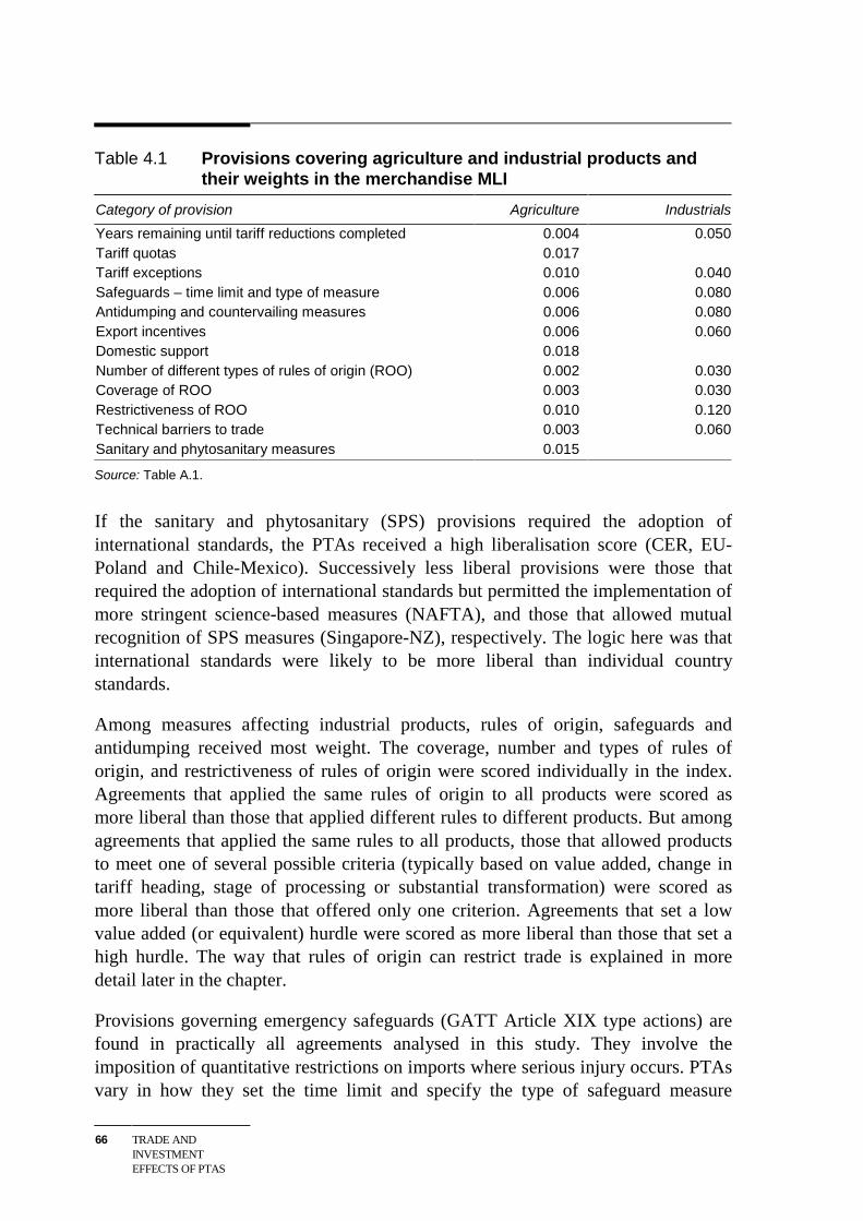
66 TRADE ANDINVESTMENTEFFECTS OF PTAS
Table 4.1 Provisions covering agriculture and industrial products andtheir weights in the merchandise MLI
Category of provision Agriculture Industrials
Years remaining until tariff reductions completed 0.004 0.050Tariff quotas 0.017Tariff exceptions 0.010 0.040Safeguards – time limit and type of measure 0.006 0.080Antidumping and countervailing measures 0.006 0.080Export incentives 0.006 0.060Domestic support 0.018Number of different types of rules of origin (ROO) 0.002 0.030Coverage of ROO 0.003 0.030Restrictiveness of ROO 0.010 0.120Technical barriers to trade 0.003 0.060Sanitary and phytosanitary measures 0.015
Source: Table A.1.
If the sanitary and phytosanitary (SPS) provisions required the adoption ofinternational standards, the PTAs received a high liberalisation score (CER, EU-Poland and Chile-Mexico). Successively less liberal provisions were those thatrequired the adoption of international standards but permitted the implementation ofmore stringent science-based measures (NAFTA), and those that allowed mutualrecognition of SPS measures (Singapore-NZ), respectively. The logic here was thatinternational standards were likely to be more liberal than individual countrystandards.
Among measures affecting industrial products, rules of origin, safeguards andantidumping received most weight. The coverage, number and types of rules oforigin, and restrictiveness of rules of origin were scored individually in the index.Agreements that applied the same rules of origin to all products were scored asmore liberal than those that applied different rules to different products. But amongagreements that applied the same rules to all products, those that allowed productsto meet one of several possible criteria (typically based on value added, change intariff heading, stage of processing or substantial transformation) were scored asmore liberal than those that offered only one criterion. Agreements that set a lowvalue added (or equivalent) hurdle were scored as more liberal than those that set ahigh hurdle. The way that rules of origin can restrict trade is explained in moredetail later in the chapter.
Provisions governing emergency safeguards (GATT Article XIX type actions) arefound in practically all agreements analysed in this study. They involve theimposition of quantitative restrictions on imports where serious injury occurs. PTAsvary in how they set the time limit and specify the type of safeguard measure
NEW EVIDENCE ONTRADE CREATIONAND DIVERSION
67
applied. In the case of a serious injury, members may suspend preferences for aperiod of one year (LAIA, Chile-Mexico) or two years (MERCOSUR, Andean). Inthe case of a serious injury, some PTAs even have provisions to suspend thepreferences until such time as the threat is no longer perceived (SPARTECA,PATCRA). However, safeguard measures are prohibited in some recent bilateralagreements — Singapore-NZ and Chile-MERCOSUR. These PTAs received a highliberalisation score for safeguard provisions. If safeguards imposed are less than oneyear and the type of measure is specified (ie transparent) — typically a quota orsuspension of preferences — then those PTAs received a higher score. If thesafeguard provisions are not transparent they received a low score. Note that thisscoring reflects how the safeguard provisions are written, not whether they are used.
Most of the PTAs analysed in this study contain provisions permitting theapplication of antidumping duties and countervailing measures in intra-PTA trade,though these are more common in free trade areas than customs unions. Theseprovisions are scored as highly liberal if they completely prohibit antidumping as aninstrument to protect member industries. Provisions requiring consistency with theWTO rules, consultation with other members, or no restrictions on the use ofantidumping and countervailing duties were scored as progressively less liberal.Those PTAs making specific reference to the GATT/WTO definition of dumpinginclude Chile-MERCOSUR and Singapore-New Zealand. Those calling forconsultations between parties prior to the adoption of protective measures includeEU and NAFTA.
Other provisions affecting both agricultural and industrial products were thosegoverning technical barriers to trade, export incentives and tariff exceptions. Undertechnical barriers to trade, initiatives to promote harmonisation of standards werescored as less liberal than national treatment of standards, voluntary recognition oftest results or full harmonisation of standards.3 Provisions to prohibit exportincentives were scored as more liberal than provisions to review them. Agreementswith fewer tariff exceptions were scored as more liberal than those with more.Provisions governing other types of subsidies on industrial goods were not includedin the index because they did not feature in most of the PTAs examined.
3 Provisions governing mutual recognition of labour market qualifications were not included in the
index because they did not feature in most of the PTAs examined (and hence, their effects wouldnot be identified precisely in the econometrics). Dispute resolution was not included, because itwas not clear what constituted a more liberal rather than a less liberal regime. This aspect ofPTAs, more than most, depends on how the facility is used, rather than how it is specified onpaper (the basis for scoring in the MLI). Tax harmonisation was not included because it did notfeature in the particular PTAs examined, although it has been the subject of separate doubletaxation agreements.
68 TRADE ANDINVESTMENTEFFECTS OF PTAS
Finally, recognition was given to the prospective nature of the tariff provisions insome more recent agreements, and hence the likelihood of them having a limitedeffect on current (though not necessarily future) trade flows. This was done byscoring the more prospective agreements as being less liberal currently than thosewhose tariff provisions were fully implemented.
The provisions indexed in the MLI are treated as additive to, and independent ofeach other. In reality some provisions might interact to strengthen or weaken otherprovisions. For example, the time schedule for preferential tariff liberalisation isclosely related to the restrictiveness of rules of origin. The impact of interactioneffects among the provisions in various PTAs is potentially an empirical question,but interaction effects have not been allowed for specifically in the construction ofthis index. For this reason, the econometrics may understate (where interactioneffects reinforce) or overstate (where interaction effects cancel) the overall effectsof PTAs. This possibility is discussed later in the chapter
The estimated relationship between provisions related to trade and the level of tradeprovide an indication of whether trade provisions included in PTAs have any effectcollectively on trade flows with member or non-member countries. Since PTAs areby definition exclusive and discriminatory against non-members, trade and non-trade provisions that are favourable to the intra-PTA trade may become barriers tonon-member countries. This effect is tested for separately.
PTA specific variables
There are two ways the merchandise MLI has been introduced into the gravitymodel. Firstly, dynamic PTA-specific indexes are defined to take a non-zero valueonly for the years in which a PTA between the two countries is in force, and to takea value of zero otherwise. These indexes capture the effect of the formation,expansion and contraction of a PTA on trade and investment only after it occurs.The membership status of the countries in each PTA is reported in the table 4.2.
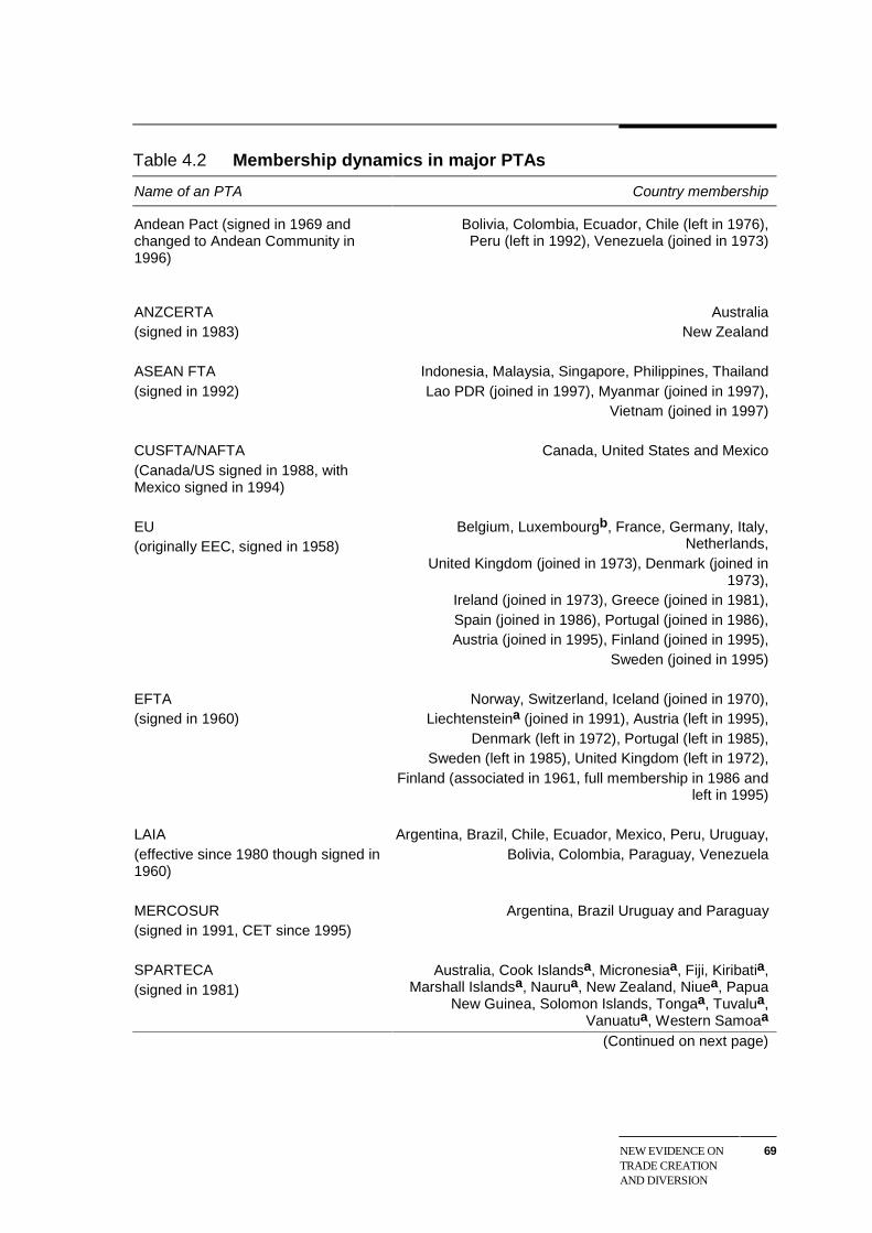
NEW EVIDENCE ONTRADE CREATIONAND DIVERSION
69
Table 4.2 Membership dynamics in major PTAs
Name of an PTA Country membership
Andean Pact (signed in 1969 andchanged to Andean Community in1996)
Bolivia, Colombia, Ecuador, Chile (left in 1976),Peru (left in 1992), Venezuela (joined in 1973)
ANZCERTA(signed in 1983)
AustraliaNew Zealand
ASEAN FTA(signed in 1992)
Indonesia, Malaysia, Singapore, Philippines, ThailandLao PDR (joined in 1997), Myanmar (joined in 1997),
Vietnam (joined in 1997)
CUSFTA/NAFTA(Canada/US signed in 1988, withMexico signed in 1994)
Canada, United States and Mexico
EU(originally EEC, signed in 1958)
Belgium, Luxembourgb, France, Germany, Italy,Netherlands,
United Kingdom (joined in 1973), Denmark (joined in1973),
Ireland (joined in 1973), Greece (joined in 1981),Spain (joined in 1986), Portugal (joined in 1986),Austria (joined in 1995), Finland (joined in 1995),
Sweden (joined in 1995)
EFTA(signed in 1960)
Norway, Switzerland, Iceland (joined in 1970),Liechtensteina (joined in 1991), Austria (left in 1995),
Denmark (left in 1972), Portugal (left in 1985),Sweden (left in 1985), United Kingdom (left in 1972),
Finland (associated in 1961, full membership in 1986 andleft in 1995)
LAIA(effective since 1980 though signed in1960)
Argentina, Brazil, Chile, Ecuador, Mexico, Peru, Uruguay,Bolivia, Colombia, Paraguay, Venezuela
MERCOSUR(signed in 1991, CET since 1995)
Argentina, Brazil Uruguay and Paraguay
SPARTECA(signed in 1981)
Australia, Cook Islandsa, Micronesiaa, Fiji, Kiribatia,Marshall Islandsa, Naurua, New Zealand, Niuea, Papua
New Guinea, Solomon Islands, Tongaa, Tuvalua,Vanuatua, Western Samoaa
(Continued on next page)
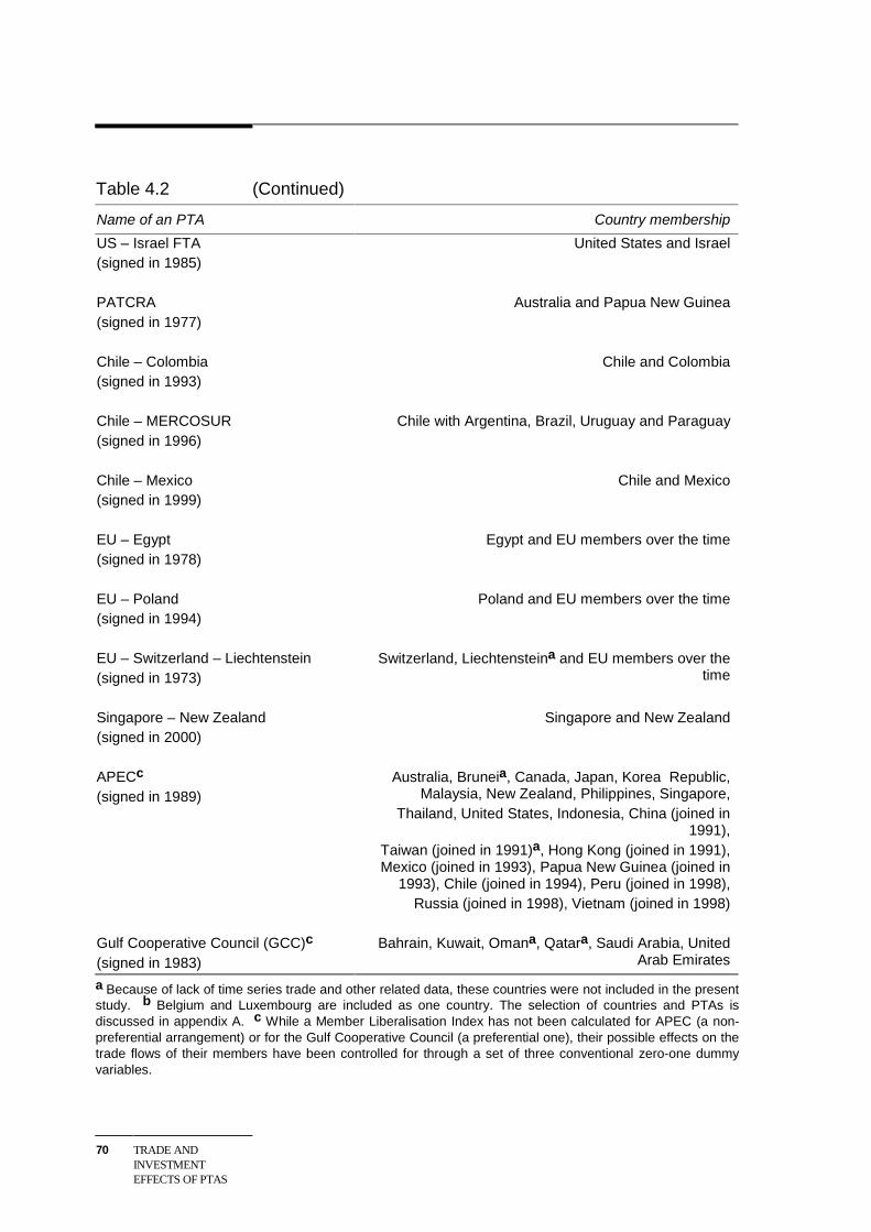
70 TRADE ANDINVESTMENTEFFECTS OF PTAS
Table 4.2 (Continued)
Name of an PTA Country membership
US – Israel FTA(signed in 1985)
United States and Israel
PATCRA(signed in 1977)
Australia and Papua New Guinea
Chile – Colombia(signed in 1993)
Chile and Colombia
Chile – MERCOSUR(signed in 1996)
Chile with Argentina, Brazil, Uruguay and Paraguay
Chile – Mexico(signed in 1999)
Chile and Mexico
EU – Egypt(signed in 1978)
Egypt and EU members over the time
EU – Poland(signed in 1994)
Poland and EU members over the time
EU – Switzerland – Liechtenstein(signed in 1973)
Switzerland, Liechtensteina and EU members over thetime
Singapore – New Zealand(signed in 2000)
Singapore and New Zealand
APECc
(signed in 1989)Australia, Bruneia, Canada, Japan, Korea Republic,
Malaysia, New Zealand, Philippines, Singapore,Thailand, United States, Indonesia, China (joined in
1991),Taiwan (joined in 1991)a, Hong Kong (joined in 1991),Mexico (joined in 1993), Papua New Guinea (joined in
1993), Chile (joined in 1994), Peru (joined in 1998),Russia (joined in 1998), Vietnam (joined in 1998)
Gulf Cooperative Council (GCC)c
(signed in 1983)Bahrain, Kuwait, Omana, Qatara, Saudi Arabia, United
Arab Emirates
a Because of lack of time series trade and other related data, these countries were not included in the presentstudy. b Belgium and Luxembourg are included as one country. The selection of countries and PTAs isdiscussed in appendix A. c While a Member Liberalisation Index has not been calculated for APEC (a non-preferential arrangement) or for the Gulf Cooperative Council (a preferential one), their possible effects on thetrade flows of their members have been controlled for through a set of three conventional zero-one dummyvariables.
NEW EVIDENCE ONTRADE CREATIONAND DIVERSION
71
In contrast, the second type is called an antimonde PTA-specific index, and it takesa non-zero value for all the years in the sample, irrespective of when the PTA wasformed. The antimonde index is used as a panel data analogue to the non-dynamicindexes of the cross sectional studies reported in chapter 3. It has the samedisadvantage of allowing the formation, expansion, contraction of a PTA to affecttrade and investment ‘before the event’.
To some extent, the choice of a starting date for PTAs is arbitrary. In some PTAs,such as EU–Poland, provisions are to be phased in slowly after implementation. Inothers, such as the EC, the generosity of the provisions has varied substantially overtime. Both issues are discussed in more detail in appendix A. Some PTAs, such asCUSTFA and CER, merely strengthened and broadened preferential accessarrangements that were already in place.
It is also possible for PTAs to affect trade and investment flows beforeimplementation, especially if the PTA formation is expected or announced well inadvance. The investment booms that occurred in Spain and Portugal prior to theiraccession to the EU are a good example of this phenomenon.
Despite this arbitrariness, the use of dynamic dummies allows a formal statisticaltest of whether the strength of trade effects associated with PTAs has beensignificantly different, on average, in the years following implementation (when thedynamic PTA dummies take zero values), compared with the effects, on average, inthe years prior to implementation (when the dynamic PTA dummies take non-zerovalues). This remains a relevant policy question.
Three PTA-specific variables for each PTA have been introduced in this study, as inSoloaga and Winters (2001), to capture the separate effects on intra-PTA trade, onimports from non-members, and on exports to non-members.
Cross sectional and panel analysis
There are two distinct advantages that a panel data model offers over the traditionalcross sectional analysis. First, a panel data model is able to capture both crosssection and time series variation in the dependent variable under investigation.Second, a panel data model is able to measure not only the effects that observablevariables have on the dependent variable, but can also control for the effects ofrelevant but unobservable or non-measurable heterogeneity across countries or overtime.
72 TRADE ANDINVESTMENTEFFECTS OF PTAS
The observable variables are the bilateral trade determinants normally included inthe gravity model. The means by which the unobservable variables are controlledfor depends upon whether a fixed effects or random effects model is used.
A fixed effects model is chosen here over a random effects model. In a randomeffects model, the unobservable effects are assumed to be uncorrelated with theobserved explanatory variables, and this is highly unlikely to be the case inpractice.4 In a fixed effects model, unobservable specific effects are assumed to befixed parameters (akin to constant terms). They can be estimated directly, so onlyweak prior assumptions are needed about their relationship with the explanatoryvariables, in contrast to the random effects specification.
Harris and Matyas (2001), Egger (2000) and Matyas (1997, 1998) have showed thatwithout controlling for unobserved heterogeneity, the parameter estimates ofinterest — the PTA effects — in the gravity model might be inflated or deflatedartificially by this misspecification. This is a type of omitted variable bias.
4.2 Model specification
Many gravity model analysts have previously excluded data on potential tradingpartners when the value of trade was zero. The bias created from such exclusion islikely to cast doubt on the validity of the findings, particularly the normality of thebehaviour of countries defined in the gravity model. This exclusion over-emphasises the effect of those countries that have positive trade flows.
This study has included information on all potential trading partners of 116countries (see appendix B for countries in the full sample), even when the countryunder investigation has no exports to the potential trading partners in some years.Since the nature of trade relations in many countries in the World Trade Flows(1997, 2000) database is such that each country trades with a relatively smallnumber of partners, the dependent variable contains a significant number of zeroobservations as well as many positive observations. For the full sample, the numberof observations is 116 countries x 115 partners x 28 years = 373520, with about 44per cent having zero values. As a result, a Tobit estimation procedure is used toappropriately account for the censored nature of the dependent variable — thenatural log of exports between country i and country j in year t.5 Tobit estimation
4 In addition, a Hausman test rejected the random effects specification. See appendix C for details,
and for additional discussion about the econometric issues associated with including fixedeffects.
5 There are a variety of alternate approaches to this problem. The zero values can be simplyomitted as in the case of Frankel (1997), which leads to the possibility of selectivity bias.
NEW EVIDENCE ONTRADE CREATIONAND DIVERSION
73
recognises that if the dependent variable is censored, then the distribution of theerror terms will be truncated, and the estimator is constructed accordingly (seeappendix C for more details).
The gravity model equation (4.1) estimated here allows for product differentiationat the country level. Much of the recent literature on PTAs has focused onimperfectly competitive behaviour, as discussed in chapter 2. Recognising this isimportant for two reasons:
• some economic integration has occurred among economies with almost similarstructures and large volumes of intra-industry trade; and
• there is a positive interaction between market structure and the gains fromintegration, often called the pro-competitive effects of PTAs, which the new ageagreements aim to capture.
The product differentiation model of Helpman and Krugman (1985) and Helpman(1987) is integrated into this gravity model specification (4.1). In their models, oneof the two goods is differentiated and the other is homogenous. The bilateral tradeof each country is the sum of inter- and intra-industry trade flows, with the latterbeing trade in the differentiated product. These product differentiationspecifications also provide a rationale for applying the gravity model to investmentflows (Egger 2001), as is done in the next chapter.
The corresponding reduced form of gravity model for trade is:
ijt
ijijijijijij
jijiijij
ijijijtijtij
ijtijtijttjiijt
Ln
MRTAMRTAMRTAwave
locklockIsIsCurCol
BorLinLnTarLnRERLnDis
LnSimilarLnRLFALnSGDPaLnY
ε
β
βββββββββββ
βββλγα
+
++++
++++++
+++++
++++++=
−−−− ∑∑∑315
14131211109
87654
321*
(4.1)
where
Ln is natural logarithmic transformation;
Arbitrarily small numbers can be used in place of zeros. Eichengreen and Irwin (1995) expressedthe dependent variable as )1( ijYLn + . Clark and Tavres (2000) and Soloaga and Winters (2001)used a Tobit specification for their cross sectional gravity model.
74 TRADE ANDINVESTMENTEFFECTS OF PTAS
*ijtY is the value of exports from country i to j in year t; using exports as a
dependent variable rather than total bilateral trade allows theidentification of export and import diversion separately;
iα is unobserved specific effects in exporting country i;
jγ is unobserved specific effects in importing country j;
tλ is unobserved specific effects in time period t;
ijtSGDP is the sum of bilateral GDPs of i and j in year t;
ijtRLFA is the absolute differences in GDP per capita of i and j in year t;
ijtSimilar is similarity in country size between i and j in year t in terms ofaggregate GDP;
ijDis is distance between the two largest or capital cities of countries i andj;
ijtRER is the bilateral real exchange rate between i and j in year t;
ijtTar is an average tariff rate between i and j in year t;
ijLin is a measure of linguistic similarity between i and j;
ijBor is a dummy that takes a value 1 if i and j share a land border and 0otherwise;
ijCol is a dummy that takes a value 1 if i and j have colonial linkages and 0otherwise;
ijCur is a dummy that takes a value 1 if i and j have the same currency and0 otherwise;
iIs is a dummy that takes a value 1 when i is island nations and 0otherwise;
iLock is a dummy that takes a value 1 when i is a landlocked nation and 0otherwise;
NEW EVIDENCE ONTRADE CREATIONAND DIVERSION
75
ijwave3 is an index capturing the third wave provisions of a PTA, that takes avalue of the non-merchandise MLI index if the i and j are participantsof a specific PTA in the sample and 0 otherwise;6 it also has a timedimension when defined in dynamic rather than antimonde form;
ijMRTA is an index capturing the merchandise trade provisions of a PTA, thattakes the value of the merchandise MLI if both countries i and jbelong to the same PTA and 0 otherwise; it also has a time dimensionwhen defined in dynamic rather than antimonde form;
jiMRTA − is an index that takes the value of the merchandise MLI when theimporting country j belongs to that particular PTA and 0 otherwise; italso has a time dimension when defined in dynamic rather thanantimonde form;
ijMRTA − is an index that takes the value of the merchandise MLI when theexporting country i belongs to that particular PTA; and 0 otherwise italso has time dimension when defined in dynamic rather thanantimonde form;
ijtε is an error term.
From an econometric point of view, the iα , jγ and tλ specific effects are treated
as fixed unknown parameters. The use of three separate fixed effects is advocatedby Matyas (1997, 1998) and avoids the omitted variable bias identified by Havemanand Hummels (1998).
The expected relationship of the observed explanatory variables with bilateralexports was discussed briefly in the previous chapter.
In a model of product differentiation, countries similar in size will trade more, andthe trade will be of an intra-industry nature. The index of size similarity (Similar)captures this effect.
By contrast, traditional trade theory says that countries with dissimilar levels of percapita GDP will trade more than the countries with similar levels, where thisreflects dissimilar factor endowments. The absolute difference in the per capitaGDP between exporting and importing countries (RLFA) is included as an
6 Because of model convergence problems, the effects of new age provisions on exports to non-
members and imports from non-members could not be analysed separately.
76 TRADE ANDINVESTMENTEFFECTS OF PTAS
explanatory variable in the gravity model as a way of distinguishing the traditionalfrom the differentiated product approaches.7
The above gravity model specification includes the real exchange rate as a relevantprice variable in order to control for fluctuations in relative prices among tradingpartners. This variable is defined as the value of a unit of the exporter’s currencyrelative to the importer’s currency in purchasing power parity terms. Adepreciation of exporting country currency is expected to show positiverelationship with exports and negative relationship with outward foreign directinvestment.
The average bilateral tariff rate (Tar) is expected to show a negative relationshipwith trade. The PTA-specific indexes capture the extent of traditional and ‘new age’provisions of a PTA, but not the size of the tariff preferences thereby created.Because the bilateral tariff variable includes preferential tariffs,8 the overallmeasured effect of PTAs on trade will be split between the tariff variable and thePTA-specific indexes in specifications where both occur. To test whether thecoefficients of the PTA-specific indexes are sensitive to the inclusion of the tariffvariable, the gravity model is estimated initially without the tariff variable. It is thenre-estimated with the tariff variable for that subset of countries and time periods forwhich bilateral tariff data are available.
4.3 Main results
The equation 4.1 is estimated in a Tobit form with fixed effects. The detailed resultsare reported in table D.1. The observable effects — trade provisions of PTAs andother bilateral trade determinants — and unobservable country and time specificeffects all significantly influence the bilateral trade flows. The coefficients on theobservable effects are generally as expected. Interestingly, they support bothtraditional and product differentiation theories of trade, because similarity in sizeand differences in income per head are both associated with higher bilateral exports.
7 The specification based on product differentiation above also differs from traditional gravity
model specifications by including the sum of importing and exporting country GDPs, rather thanincluding each separately. This small loss of generality means that the product differentiationversion does not encompass the traditional model fully.
8 The bilateral tariff data are applied rates obtained from UNCTAD’s TRAINS database. As such,they incorporate tariff preferences.
NEW EVIDENCE ONTRADE CREATIONAND DIVERSION
77
Comparison with past estimates
The new estimates of trade creation and diversion tend to be different from pastestimates for most PTAs.
Past estimates showed most PTAs to be trade creating in net terms. By contrast, theresults here suggest most of the PTAs examined did not create additional trade,either for members or for non-members of the agreement.
The ‘net trade effects’ of preferential agreements found in this study are comparedwith past estimates in table 4.3, which shows whether the net effects are positive ornegative.9 The relationship between these net trade effects and welfare effects isweak (despite the ‘building block’ and ‘stumbling block’ terminology sometimesused). It was found in chapter 2 that abstracting from terms of trade effects, ifempirical tests established net trade creation, then a PTA may still have generatedwelfare losses, while if the empirical tests established net trade diversion, then thePTA cannot have created welfare gains. However, terms of trade effects couldpossibly reverse this latter conclusion for at least some PTA members.
The new estimates of net trade effects reverse most of the past findings. Nearly allPTAs are found to have caused net trade diversion in the new assessment. ThePTAs found to have inconclusive effects in past analysis drifted either way in thenew assessment, but MERCOSUR was found here to have caused net tradediversion.
Overall, the main PTAs — NAFTA, EC/EU, MERCOSUR, and CER — as well asmany bilateral agreements not considered previously, are found here to have creatednegative net trade effects. However, there is a qualification to this finding. Inagreements with a small number of members, the intra-PTA effect is estimatedimprecisely, with a large standard error, while the extra-PTA effect can beestimated more accurately.10 Thus, the findings for those PTAs, such as CER, witha small number of members are less robust than those for larger PTAs. In addition,the measures of distance used in this study are unlikely to capture fully the ways inwhich changes in trading patterns and reductions in transport costs have raised theattractiveness of extra-bloc as opposed to intra-bloc trade for CER members overtime. 9 The assessment of net trade effects is based on the marginal effects of PTAs reported in table C.1,
rather than the raw maximum likelihood Tobit estimates in table D.1, for the preferredspecification with dynamic PTA variables and fixed effects. Although the marginal effects andraw Tobit estimates are not equal (as explained in appendix C), in practice the assessment of thedirection of net trade effects is the same, whichever is used.
10 For example, the intra-CER dummy has positive values only for 14 x 15 = 210 observations andzero for remaining observations.
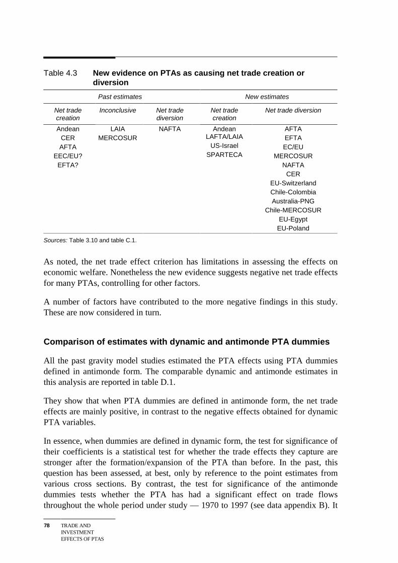
78 TRADE ANDINVESTMENTEFFECTS OF PTAS
Table 4.3 New evidence on PTAs as causing net trade creation ordiversion
Past estimates New estimates
Net tradecreation
Inconclusive Net tradediversion
Net tradecreation
Net trade diversion
AndeanCERAFTA
EEC/EU?EFTA?
LAIAMERCOSUR
NAFTA AndeanLAFTA/LAIA
US-IsraelSPARTECA
AFTAEFTAEC/EU
MERCOSURNAFTA
CEREU-SwitzerlandChile-ColombiaAustralia-PNG
Chile-MERCOSUREU-EgyptEU-Poland
Sources: Table 3.10 and table C.1.
As noted, the net trade effect criterion has limitations in assessing the effects oneconomic welfare. Nonetheless the new evidence suggests negative net trade effectsfor many PTAs, controlling for other factors.
A number of factors have contributed to the more negative findings in this study.These are now considered in turn.
Comparison of estimates with dynamic and antimonde PTA dummies
All the past gravity model studies estimated the PTA effects using PTA dummiesdefined in antimonde form. The comparable dynamic and antimonde estimates inthis analysis are reported in table D.1.
They show that when PTA dummies are defined in antimonde form, the net tradeeffects are mainly positive, in contrast to the negative effects obtained for dynamicPTA variables.
In essence, when dummies are defined in dynamic form, the test for significance oftheir coefficients is a statistical test for whether the trade effects they capture arestronger after the formation/expansion of the PTA than before. In the past, thisquestion has been assessed, at best, only by reference to the point estimates fromvarious cross sections. By contrast, the test for significance of the antimondedummies tests whether the PTA has had a significant effect on trade flowsthroughout the whole period under study — 1970 to 1997 (see data appendix B). It
NEW EVIDENCE ONTRADE CREATIONAND DIVERSION
79
does not distinguish whether the trade effects were any stronger after the PTAformation than before. This is similar to most of the (cross sectional) tests in theliterature to date.
Defining PTA dummies in dynamic form provides a more stringent statistical test ofwhether it was PTA formation, rather than some other set of factors specific to thebilateral country pair, accounting for the observed trade effects. The power of thetest is further strengthened by the fact that individual country- and time-specificeffects are controlled for separately, through the fixed effects (see also below). Themore stringent test of the before/after effects of PTAs is the major factor accountingfor the more negative findings of this study.
The differences are more prominent for the EC/EU and MERCOSUR agreements,where membership dynamics play an important role in their trade creation anddiversion effects. For example, a significant negative intra-EU effect is found whenusing dynamic dummies, compared to a significant positive effect found usingantimonde dummies. The dynamic dummies account for individual countriesswitching from EFTA to the EU.
Comparison of estimates with and without fixed effects
Another reason for the more negative findings in this study is the use of panelanalysis, which allows unobservable heterogeneity to be controlled for. As noted inappendix C, without allowing for fixed effects, the coefficients of both the PTAvariables and the other explanatory variables tend to be upward biased, as are thetest statistics for the significance of these variables (all reported in table D.1). Alikelihood-ratio test confirms the joint significance of the fixed effects.11
This suggests that inferences based on past gravity model estimates without fixedeffects suffer from omitted variable bias. Controlling for unobservableheterogeneity is another reason for the more negative findings in this study.
Comparison of estimates with and without tariffs
A model with the average bilateral tariff variable as an additional determinant oftrade is estimated on a restricted dataset,12 and the results are reported in table D.2.As noted, while the PTA dummies capture the existence of tariff preferences, the 11 The calculated test statistic of 114775.3 clearly rejects the null hypothesis, as is expected given
the individual significance of most of the country and time specific fixed effects in the model.12 The dataset is restricted because of the lack of bilateral tariff data for a number of countries and
for a number of years.
80 TRADE ANDINVESTMENTEFFECTS OF PTAS
tariff variable captures an additional effect — the height of the preferences socreated.
Results from this analysis show that the average tariff rate in the importing countryhas a significant and negative effect on its imports, as expected. The PTA dummiesalso show a significant effect. This is because they capture not just the existence oftariff preferences (as also captured by the tariff variable), but also the effects of non-tariff measures affecting merchandise trade, such as rules of origin.
The coefficients on the PTA dummies are generally not sensitive to the inclusion orexclusion of the tariff variable. So the inclusion of a tariff variable makes littledifference to the main findings of this study. But in some cases, negative intra bloctrade effects in the full sample become positive in the smaller sample. And perhapsnot surprisingly, while the comparative advantage motivation for trade showed assignificant in the full sample (with a positive and significant coefficient on thedifference in per capita GDP), this is not the case in the restricted sample. Thesedifferences also show that what constitutes ‘normal’ trade is conditioned by howmany countries and years are in the sample — those studies with restricted time andcountry coverage, particularly where it is restricted to high income developedcountries, are likely to have results biased accordingly.
The effect of third wave provisions
Third wave provisions mainly cover investment and trade in services. Investmentflows may substitute or complement exports, depending on the reasons for theexport flows (Markusen 1983).
The ‘new age’ provisions show a positive (complementary) relationship with intrabloc trade when PTA dummies are defined dynamically. Thus favourableinvestment and services trade provisions in PTAs can enhance merchandise tradebetween member countries once the agreement is in operation.
Unfortunately, it has not been possible to test whether the non-merchandise tradeprovisions of PTAs have contributed to trade diversion from non-member countries.This is because convergence problems prevented estimation when a full set of threenon-merchandise trade dummies were introduced.
The effect of bilateral versus plurilateral PTAs
A quick look at the estimated coefficients for plurilateral and bilateral agreements intable D.1 (with a dynamic specification of PTA dummies) tentatively indicates thatbilateral agreements have a more negative impact on members’ trade flows than the
NEW EVIDENCE ONTRADE CREATIONAND DIVERSION
81
plurilateral agreements. However, this finding has the same qualification aspreviously — the intra-PTA effect is estimated imprecisely, with a large standarderror, in agreements with a small number of members.
Two types of bilateral agreements are analysed in this study:
• economy to economy — CER, Chile-Colombia, US-Israel, Australia-PNG; and
• economy to PTA — EU-Egypt, EU-Poland, Chile-MERCOSUR.
Of all the bilateral agreements assessed, only the US-Israel PTA has a positiveimpact on members’ trade flows, although as explained later, this agreement is aspecial case. Apart from Chile-Colombia, all economy to economy PTAs have anadverse effect on non-members’ trade flows.
To confirm the negative effects of bilateral agreements on members’ trade flows,table D.3 reports the results of a Wald test of whether the group of coefficients on aparticular PTA index for all bilateral agreements is significantly different from zero,and similarly for plurilateral agreements. Though the null hypothesis of no effect isrejected for all three PTA indexes (intra-PTA, extra-PTA imports and extra-PTAexports) across both bilateral and plurilateral agreements, the calculated statistic isconsistently lower for bilateral PTAs than for plurilateral PTAs. This is onlycircumstantial evidence, however, and should not be considered as conclusive.
In summary, the main result is that PTAs are not as relatively benign as previousstudies have indicated. After controlling for country and time specific effects, andthe degree of liberalisation of merchandise trade provisions, in an unrestrictedsample, and testing explicitly for whether the trade effects are significantly differentafter PTA formation than before, most PTAs were estimated to have negative nettrade creation. Other recent empirical assessments have shown more optimisticoutlook for preferential agreements by ignoring these analytical issues.
4.4 Puzzles on new evidence
There are two puzzles on new evidence that need careful discussion in this study.
• The intra-bloc effect is found to be positive for the least liberal PTAs — LAIA,Andean, SPARTECA and US-Israel.
• The intra-bloc effect is found to be negative for apparently more comprehensiveand liberalised PTAs — EU, CER, NAFTA, MERCOSUR and some recentbilateral agreements.
82 TRADE ANDINVESTMENTEFFECTS OF PTAS
On the first point, the new estimates obtained in this study suggest that the leastliberal PTAs have nevertheless removed certain intra-PTA barriers or made otherchanges in these economies (not captured by the unobservable fixed effects andobserved determinants), which may have contributed to their positive intra-bloceffect.
The two Latin American PTAs are based on import substituting policies. Because ofdebt crises and balance of payment problems in early 1980s, almost all countries inLatin America underwent deep recession and a severe contraction of intra-regionaltrade. But within a very short period of time, three to five years, countries in thesePTAs revived with a mixture of unilateral reforms and a fixed margin of preferencebelow the MFN binding rates for member countries. Though the merchandise tradeprovisions were not particularly liberal, this period trade effect might havedominated, giving rise to a positive intra-PTA effect for these PTAs.
The non-reciprocal agreement with Australia and New Zealand has helped the smallisland countries of the South Pacific to transform from subsistence to more exportoriented economies. SPARTECA played an important role in stimulating exportsfrom Fiji, Solomon Islands and other island economies to Australia and NewZealand. A tuna cannery in the Solomon Islands and Fiji’s garment, footwear andfood manufacturing (SaraLee cakes) industries are all dependent on generous accessto these two developed country markets. This could partly explain the positive intra-PTA effect of SPARTECA observed in this study.
The bilateral agreement between the US and Israel is a special agreement that alsoincludes military supplies along with other merchandise trade provisions. It is theonly PTA that incorporates the whole of GATT/WTO article XXI — securityexceptions. On average, there is high trade in SITC 951 category — arms andammunitions for military supply — between the United States and Israel. This couldbe one of the possible reasons for positive intra-PTA effect observed for thisbilateral agreement.
On the second point, the highly liberalised trade provisions in many PTAsapparently had a negative impact collectively on intra-bloc trade flows of members.
One possible reason is that total elimination of tariffs among members, as requiredby GATT Article XXIV, may not be optimal for members. For example, Frankel,Stein and Wei (1995) found that a 22 per cent reduction in tariffs below multilateraltariff levels may instead be optimal. However, this finding is driven by welfareeffects, not by trade volume effects.
A more likely explanation is that, although the merchandise MLI used in this studyhas attempted to capture the potentially trade-restrictive effects of the non-tariff
NEW EVIDENCE ONTRADE CREATIONAND DIVERSION
83
merchandise trade provisions embodied in PTAs, it has not always captured themadequately.
For example, as noted earlier, the merchandise MLI has treated the trade restrictiveeffects of rules of origin as being additive to, and independent from, the otherprovisions of PTAs. In reality, not only are rules of origin restrictive, they are alsolikely to neutralise or even reverse the trade effects of other provisions that areapparently quite liberal. The sparse theoretical literature on rules of origin wassummarised in chapter 2.
The way in which rules of origin can operate in practice to counter the effects ofother provisions that are apparently quite liberal can be seen most clearly in the caseof NAFTA. There, the rules of origin are relatively complex — the specification ofrequirements for minimum change in tariff heading vary product by product, andtake up several hundred pages. Further, they are strictly enforced. The domesticcontent rules applied in the EU are also relatively complex. Even if the tariffs oneach product are eliminated entirely (an apparently quite liberal provision), thecomplex rules of origin governing the sourcing of inputs to qualify for the tariffconcession on output can undo the liberal effect of the tariff concession on output.This is not recognised in the MLI, which treats tariff provisions and rules of originadditively, not interactively. Thus the MLI may overstate the effective amount ofliberalisation in agreements with complex rules of origin, explaining why it was theapparently more comprehensive and liberalised PTAs that were found to have anegative intra-bloc effect.
Further, the MLI does not capture two final aspects of rules of origin. The first isthe way in which they can multiply distortions as overlapping PTAs begin to form.Panagariya (1999, p. 489) gives the following example:
… if Chile, who already has an FTA [free trade agreement] with MERCOSUR, joinsNAFTA, a Chilean firm will have to buy components in Brazil if it wants to takeadvantage of the preferential tariff in MERCOSUR and in the United States if it wantsto exploit the preference in NAFTA. This is notwithstanding the fact that the mostefficient supplier of the components might be in Asia.
The second is that, in a political economy context, rules of origin can becomeanother instrument for sectional interests to add to trade diversion and frustratetrade creation. This in turn explains their prevalence and complexity in agreementssuch as NAFTA.
Similarly, the speed of implementation of tariff cuts has been treated as independentfrom the coverage of those cuts. In reality, the backsliding that has occurred inMERCOSUR is likely to make that agreement less liberal than the merchandiseMLI suggests.
84 TRADE ANDINVESTMENTEFFECTS OF PTAS
As already noted, the control variables used in this study are unlikely to capturefully the way that reductions in transport costs have raised the attractiveness ofextra-bloc as opposed to intra-bloc trade for CER members over time.
Finally, there has been significant unilateral, non-discriminatory liberalisationthroughout the world, but particularly in parts of Asia and Latin America, over theperiod of study. This would have been expected to boost trade with both membersand non-members in absolute terms, and played an important part in defining thebenchmark of ‘normal trade’ against which PTAs have been assessed. The PTAdummies test whether the changes in block members’ trade patterns have beensignificantly different from those on average across the entire sample of countries.The results suggest that in may cases, this has not been the case.
4.5 Summary
This chapter has used recent bilateral trade data to provide new estimates of thetrade effects of the merchandise trade provisions included in various PTAs.
The empirical results indicate that the merchandise trade provisions in various PTAshave generally diverted more trade than they have created. Some of the moreprominent PTAs have not even succeed in creating more trade among members.
These findings are more adverse than those of other recent studies. The main reasonis that this study undertakes an explicit statistical test for whether the trade effectsof PTAs are different after PTA formation than before. In the past, this question hasbeen assessed, at best, only by reference to the point estimates from various crosssections. In addition, this study controls for a broader range of observable factorsaffecting bilateral trade flows, as well as for unobserved differences acrosscountries and time periods. It thus avoids the biases in the estimated effects of PTAsintroduced by omitting these variables. It uses a dataset in which the sample ofcountries and time periods is as large as possible, thus avoiding biasing thebenchmark of ‘normal trade’ against which PTAs are assessed. Finally, this studyalso recognises the varying breadth of coverage of the merchandise provisions invarious PTAs. Nevertheless, some aspects, particularly the trade restricting natureof rules of origin and the importance of delayed timing of tariff reductions, have notbeen captured adequately.
Finally, the results suggest that the non-merchandise trade provisions of PTAs,covering such things as investment and services, have had a positive impact onmerchandise trade flows among members. Unfortunately, for econometric reasons,it has not been possible to test whether these non-merchandise trade provisions havecontributed to trade diversion from non-member countries. But the next chapter
NEW EVIDENCE ONTRADE CREATIONAND DIVERSION
85
examines the effects of those non- merchandise trade provisions on flows of foreigndirect investment.

86 TRADE ANDINVESTMENTEFFECTS OF PTAS
INVESTMENTCREATION ANDDIVERSION
87
5 Investment creation and diversion
This chapter provides new evidence on the effects of PTAs on investment. In doingso, it takes account of the analytical issues described in chapter 4.
The bilateral investment data for this analysis are sourced from UNCTAD andOECD for the period between 1988 and 1997 for about 77 countries. These dataallow an examination of the investment effects of ten PTAs, a more restricted setthan in the previous chapter. As there are some deficiencies in the investment data(appendix B), the qualitative aspects of the analytical results rather than the precisemagnitude of the estimates are of main interest.
Apart from the more limited number of years and countries analysed, the model inthis chapter is similar to the one in the previous chapter. The sign and magnitude ofthe impact of some explanatory variables may differ, but many bilateraldeterminants are similar for trade and investment (see also Egger 2001).
The ‘new age’ provisions covered in each PTA are discussed in next section,followed by model specification. Results from the gravity model are discussed insection 5.3 and the final section summarises the key findings.
5.1 ‘New age’ or third wave provisions in PTAs
PTAs vary in their coverage of various ‘new age’ provisions. A non-merchandiseMember Liberalisation Index has been calculated, which captures this variation. Ahigh index indicates that a PTA is more liberal to members in its services trade,investment and related provisions. These provisions, along with their weights in theindex, are listed in table 5.1. The index takes a high value for Singapore-NZ,1
followed by CER, NAFTA, EU, and MERCOSUR (see tables A.1 and A.2).
A PTA that is voluntary has been scored as less liberal than one that is binding. Allpreferential PTAs examined in this study received a high score for this category.
1 The agreement was signed in 2000. Bilateral FDI data are available only up to 1997. Therefore,
the effects of this agreement on investment are not analysed in this study.
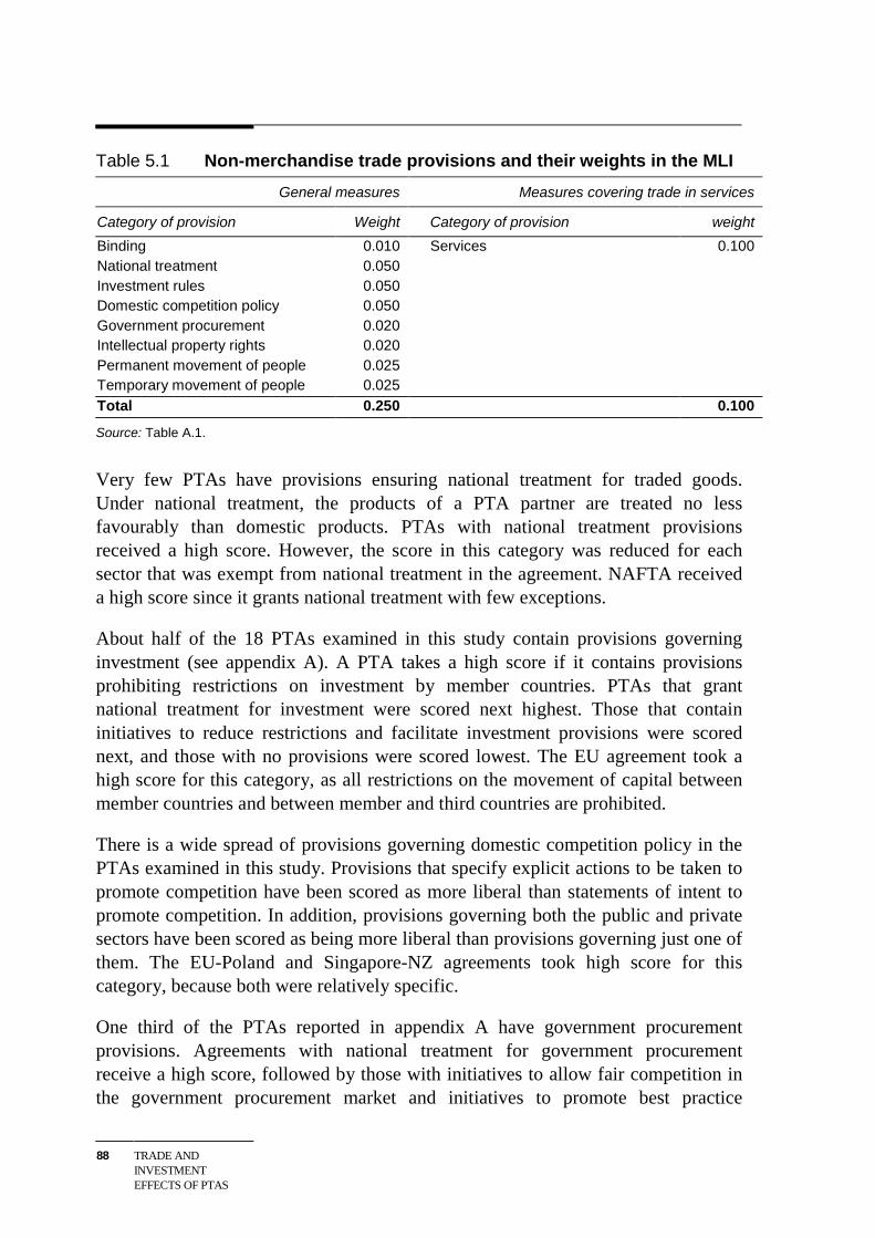
88 TRADE ANDINVESTMENTEFFECTS OF PTAS
Table 5.1 Non-merchandise trade provisions and their weights in the MLI
General measures Measures covering trade in services
Category of provision Weight Category of provision weight
Binding 0.010 Services 0.100National treatment 0.050Investment rules 0.050Domestic competition policy 0.050Government procurement 0.020Intellectual property rights 0.020Permanent movement of people 0.025Temporary movement of people 0.025Total 0.250 0.100
Source: Table A.1.
Very few PTAs have provisions ensuring national treatment for traded goods.Under national treatment, the products of a PTA partner are treated no lessfavourably than domestic products. PTAs with national treatment provisionsreceived a high score. However, the score in this category was reduced for eachsector that was exempt from national treatment in the agreement. NAFTA receiveda high score since it grants national treatment with few exceptions.
About half of the 18 PTAs examined in this study contain provisions governinginvestment (see appendix A). A PTA takes a high score if it contains provisionsprohibiting restrictions on investment by member countries. PTAs that grantnational treatment for investment were scored next highest. Those that containinitiatives to reduce restrictions and facilitate investment provisions were scorednext, and those with no provisions were scored lowest. The EU agreement took ahigh score for this category, as all restrictions on the movement of capital betweenmember countries and between member and third countries are prohibited.
There is a wide spread of provisions governing domestic competition policy in thePTAs examined in this study. Provisions that specify explicit actions to be taken topromote competition have been scored as more liberal than statements of intent topromote competition. In addition, provisions governing both the public and privatesectors have been scored as being more liberal than provisions governing just one ofthem. The EU-Poland and Singapore-NZ agreements took high score for thiscategory, because both were relatively specific.
One third of the PTAs reported in appendix A have government procurementprovisions. Agreements with national treatment for government procurementreceive a high score, followed by those with initiatives to allow fair competition inthe government procurement market and initiatives to promote best practice
INVESTMENTCREATION ANDDIVERSION
89
procurement procedures. The CER and NAFTA agreements took a high score forthis category, followed by Singapore-NZ.
Many PTAs also include provisions related to intellectual property rights.Provisions for adequate and effective protection, national treatment for propertyrights and no provisions were scored as being successively less liberal. NAFTA hasnational treatment for property rights.
Very few PTAs include provisions governing the permanent and temporarymovement of people. Where free movement is allowed it is scored as most liberal,with initiatives to promote movement of people and no provisions being scoredsuccessively lower. The EU and CER agreements received a high score for thiscategory, followed by the EU-Poland and Singapore-NZ agreements.
Of the 18 PTAs reported in appendix A, 11 cover services trade. Some agreementsadopt the GATS model of a ‘positive list’ — countries undertake national treatmentand market access commitments only in scheduled sectors. Other adopt the NAFTAmodel of a ‘negative list’ — all sectors and measures are to be liberalised unlessotherwise specified in annexes containing reservations, or non-confirmingmeasures. Non-confirming measures in the annexes are then usually liberalisedthrough consultations or periodic negotiations. The ‘negative list’ is moretransparent because it forces governments to reveal all non-confirming measuresand excluded sectors.
The ‘positive list’ model is adopted mainly by developing country PTAs — AFTAand MERCOSUR — to open their services markets gradually. The ‘negative list’model is adopted in more recent PTAs in both developing and developed countries— CER, Singapore-NZ and Chile-Mexico. The PTAs that follow the ‘positive list’model receive a lower score than those that follow the ‘negative list’ model.
If an agreement has provisions for market access and national treatment for servicestrade, it receives a high score (CER and Singapore-NZ). This was followed byagreement with provisions for market access only, provisions for national treatmentonly, and initiatives to promote services liberalisation.
The PTAs analysed in this study have been scored on the degree of theircommitment to the above elements of the agreement. The effects of these provisionson non-member countries mainly depend on the nature and the extent ofdiscrimination against non-member investors or goods and services providers.
The index of ‘new age’ provisions is included in the gravity model to study theirimpact on members’ investment in both other member and non-member countries.
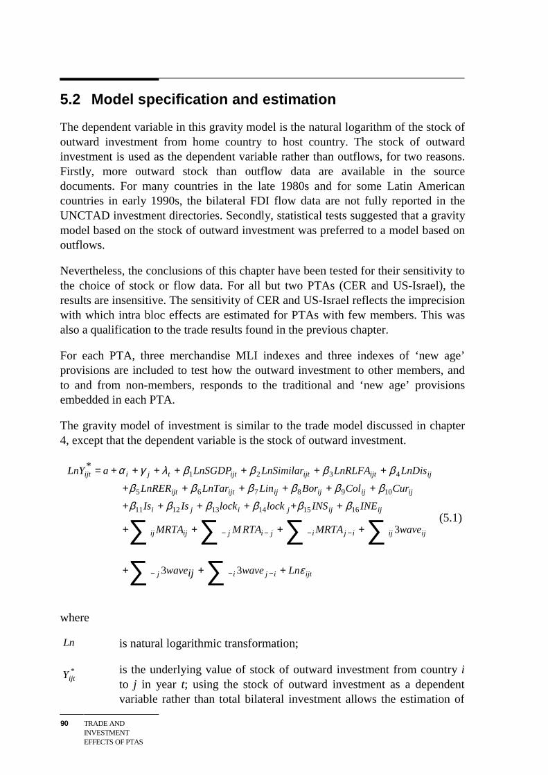
90 TRADE ANDINVESTMENTEFFECTS OF PTAS
5.2 Model specification and estimation
The dependent variable in this gravity model is the natural logarithm of the stock ofoutward investment from home country to host country. The stock of outwardinvestment is used as the dependent variable rather than outflows, for two reasons.Firstly, more outward stock than outflow data are available in the sourcedocuments. For many countries in the late 1980s and for some Latin Americancountries in early 1990s, the bilateral FDI flow data are not fully reported in theUNCTAD investment directories. Secondly, statistical tests suggested that a gravitymodel based on the stock of outward investment was preferred to a model based onoutflows.
Nevertheless, the conclusions of this chapter have been tested for their sensitivity tothe choice of stock or flow data. For all but two PTAs (CER and US-Israel), theresults are insensitive. The sensitivity of CER and US-Israel reflects the imprecisionwith which intra bloc effects are estimated for PTAs with few members. This wasalso a qualification to the trade results found in the previous chapter.
For each PTA, three merchandise MLI indexes and three indexes of ‘new age’provisions are included to test how the outward investment to other members, andto and from non-members, responds to the traditional and ‘new age’ provisionsembedded in each PTA.
The gravity model of investment is similar to the trade model discussed in chapter4, except that the dependent variable is the stock of outward investment.
ijtijij
ijijijijijijij
ijijjiji
ijijijijijtijt
ijijtijtijttjiijt
Lnwaveijwave
waveMRTARTAMMRTA
INEINSlocklockIsIs
CurColBorLinLnTarLnRER
LnDisLnRLFALnSimilarLnSGDPaLnY
ε
ββββββββββββ
ββββλγα
+++
++++
++++++
++++++
+++++++=
−−−
−−−−
∑∑∑∑∑∑
33
3
*
161514131211
1098765
4321
(5.1)
where
Ln is natural logarithmic transformation;
*ijtY is the underlying value of stock of outward investment from country i
to j in year t; using the stock of outward investment as a dependentvariable rather than total bilateral investment allows the estimation of
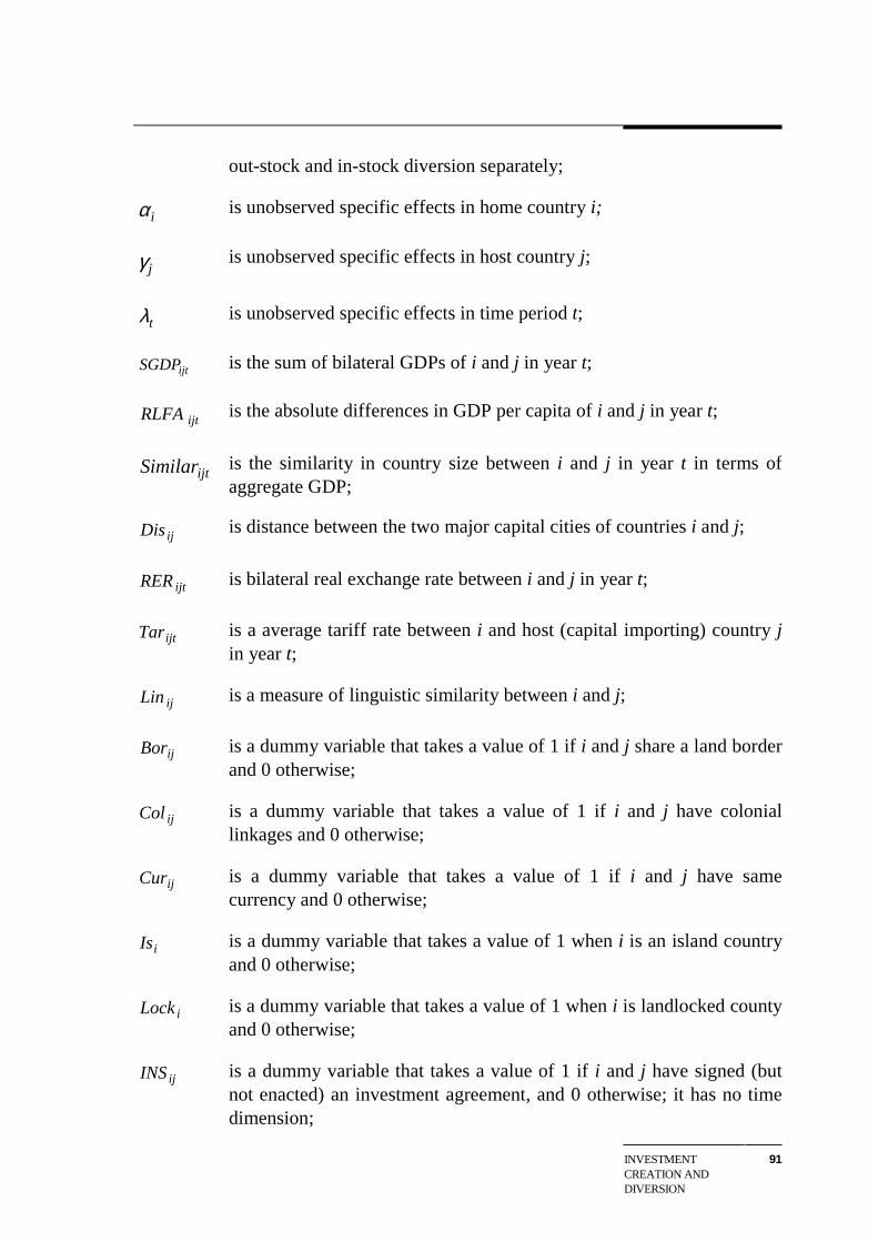
INVESTMENTCREATION ANDDIVERSION
91
out-stock and in-stock diversion separately;
iα is unobserved specific effects in home country i;
jγ is unobserved specific effects in host country j;
tλ is unobserved specific effects in time period t;
ijtSGDP is the sum of bilateral GDPs of i and j in year t;
ijtRLFA is the absolute differences in GDP per capita of i and j in year t;
ijtSimilar is the similarity in country size between i and j in year t in terms ofaggregate GDP;
ijDis is distance between the two major capital cities of countries i and j;
ijtRER is bilateral real exchange rate between i and j in year t;
ijtTar is a average tariff rate between i and host (capital importing) country jin year t;
ijLin is a measure of linguistic similarity between i and j;
ijBor is a dummy variable that takes a value of 1 if i and j share a land borderand 0 otherwise;
ijCol is a dummy variable that takes a value of 1 if i and j have coloniallinkages and 0 otherwise;
ijCur is a dummy variable that takes a value of 1 if i and j have samecurrency and 0 otherwise;
iIs is a dummy variable that takes a value of 1 when i is an island countryand 0 otherwise;
iLock is a dummy variable that takes a value of 1 when i is landlocked countyand 0 otherwise;
ijINS is a dummy variable that takes a value of 1 if i and j have signed (butnot enacted) an investment agreement, and 0 otherwise; it has no timedimension;
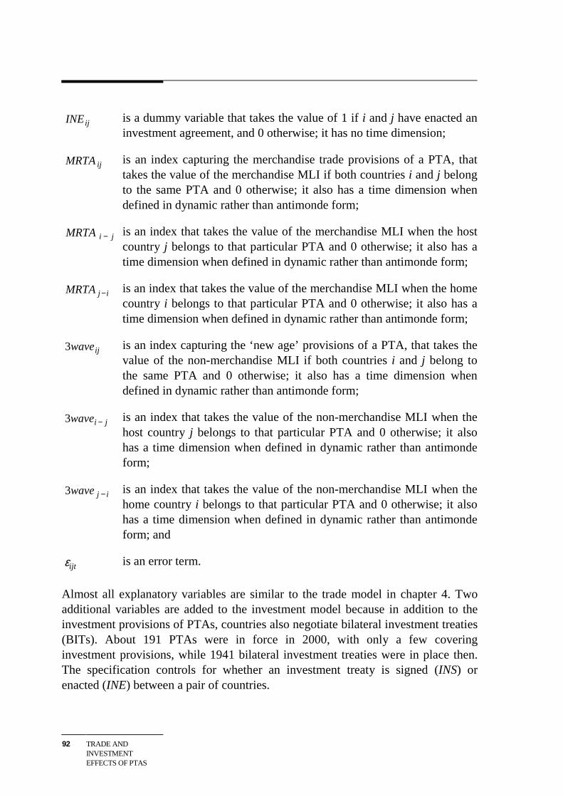
92 TRADE ANDINVESTMENTEFFECTS OF PTAS
ijINE is a dummy variable that takes the value of 1 if i and j have enacted aninvestment agreement, and 0 otherwise; it has no time dimension;
ijMRTA is an index capturing the merchandise trade provisions of a PTA, thattakes the value of the merchandise MLI if both countries i and j belongto the same PTA and 0 otherwise; it also has a time dimension whendefined in dynamic rather than antimonde form;
jiMRTA − is an index that takes the value of the merchandise MLI when the hostcountry j belongs to that particular PTA and 0 otherwise; it also has atime dimension when defined in dynamic rather than antimonde form;
ijMRTA − is an index that takes the value of the merchandise MLI when the homecountry i belongs to that particular PTA and 0 otherwise; it also has atime dimension when defined in dynamic rather than antimonde form;
ijwave3 is an index capturing the ‘new age’ provisions of a PTA, that takes thevalue of the non-merchandise MLI if both countries i and j belong tothe same PTA and 0 otherwise; it also has a time dimension whendefined in dynamic rather than antimonde form;
jiwave −3 is an index that takes the value of the non-merchandise MLI when thehost country j belongs to that particular PTA and 0 otherwise; it alsohas a time dimension when defined in dynamic rather than antimondeform;
ijwave −3 is an index that takes the value of the non-merchandise MLI when thehome country i belongs to that particular PTA and 0 otherwise; it alsohas a time dimension when defined in dynamic rather than antimondeform; and
ijtε is an error term.
Almost all explanatory variables are similar to the trade model in chapter 4. Twoadditional variables are added to the investment model because in addition to theinvestment provisions of PTAs, countries also negotiate bilateral investment treaties(BITs). About 191 PTAs were in force in 2000, with only a few coveringinvestment provisions, while 1941 bilateral investment treaties were in place then.The specification controls for whether an investment treaty is signed (INS) orenacted (INE) between a pair of countries.
INVESTMENTCREATION ANDDIVERSION
93
Apart from the real exchange rate, the expected relationship of the normal bilateralinvestment determinants with outward investment is the same as in the tradeequation of the previous chapter. The real exchange rate (RER) is expected to showa negative effect on outward investment in the short term as depreciation of thehome country currency rate reduces home country production costs relative toforeign production costs. It therefore increases labour demand and employment andraises the return on capital in the home country, increasing domestic investment atthe expense of outward FDI.
The effects of traditional and ‘new age’ provisions on investment are lessstraightforward.
If trade liberalisation makes exporting from the home country relatively moreattractive than FDI as a way to serve the regional market, then the trade provisionsof a PTA could cause a reduction in intra-bloc investment. But the trade provisionscould also enable transnational corporations (TNC) to operate vertically in a PTAarea, stimulating intra-FDI flows among the relevant partners. The structure andmotivation of investment will determine the net impact of trade provisions of PTAson intra-PTA investment. So too will the structure and motivation of intra-bloc trade(Markusen 1983).
According to Ethier (1998, 2001) the inflows of FDI from non-member countriesinto the PTA region are likely to go up in response to the trade provisions of PTAs,as non-members establish beachhead position in one PTA member country in orderto serve the market of the others. Alternatively, if multinationals are initiallyoperating in member countries to serve the protected local market (the tariffjumping motivation for investment), then these multinationals may rationalise theirnetwork of affiliates after the formation of the PTA and as a result, some membercountries could lose investment to non-member countries.
Thus, the response of investment to the merchandise trade provisions of a PTA is anempirical question. The various possibilities can be tested in the following way.
If investment responds in beachhead fashion to the trade provisions of PTAs and inturn stimulates intra-bloc trade, this can be identified by the combination of apositive and significant effect of trade provisions on intra-bloc trade and a positiveand significant effect of trade provisions on investment from non-member countries(a positive coefficient on jiMRTA − in equation 5.1).
Alternatively, a reversal of tariff jumping investment can be identified by a positiveand significant effect of trade provisions on investment to non-member countries (apositive coefficient on ijMRTA − in equation 5.1).
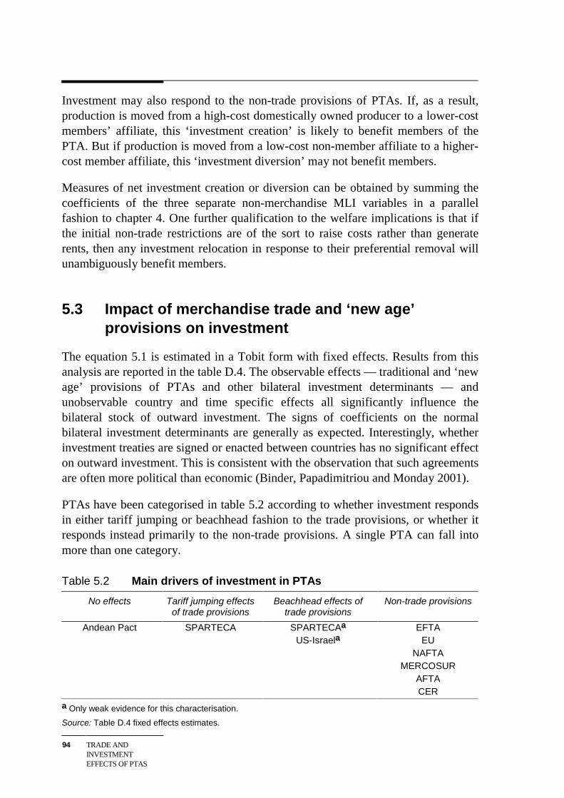
94 TRADE ANDINVESTMENTEFFECTS OF PTAS
Investment may also respond to the non-trade provisions of PTAs. If, as a result,production is moved from a high-cost domestically owned producer to a lower-costmembers’ affiliate, this ‘investment creation’ is likely to benefit members of thePTA. But if production is moved from a low-cost non-member affiliate to a higher-cost member affiliate, this ‘investment diversion’ may not benefit members.
Measures of net investment creation or diversion can be obtained by summing thecoefficients of the three separate non-merchandise MLI variables in a parallelfashion to chapter 4. One further qualification to the welfare implications is that ifthe initial non-trade restrictions are of the sort to raise costs rather than generaterents, then any investment relocation in response to their preferential removal willunambiguously benefit members.
5.3 Impact of merchandise trade and ‘new age’provisions on investment
The equation 5.1 is estimated in a Tobit form with fixed effects. Results from thisanalysis are reported in the table D.4. The observable effects — traditional and ‘newage’ provisions of PTAs and other bilateral investment determinants — andunobservable country and time specific effects all significantly influence thebilateral stock of outward investment. The signs of coefficients on the normalbilateral investment determinants are generally as expected. Interestingly, whetherinvestment treaties are signed or enacted between countries has no significant effecton outward investment. This is consistent with the observation that such agreementsare often more political than economic (Binder, Papadimitriou and Monday 2001).
PTAs have been categorised in table 5.2 according to whether investment respondsin either tariff jumping or beachhead fashion to the trade provisions, or whether itresponds instead primarily to the non-trade provisions. A single PTA can fall intomore than one category.
Table 5.2 Main drivers of investment in PTAs
No effects Tariff jumping effectsof trade provisions
Beachhead effects oftrade provisions
Non-trade provisions
Andean Pact SPARTECA SPARTECAa
US-IsraelaEFTA
EUNAFTA
MERCOSURAFTACER
a Only weak evidence for this characterisation.
Source: Table D.4 fixed effects estimates.
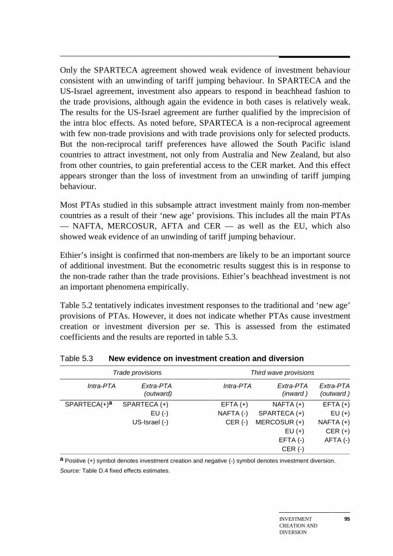
INVESTMENTCREATION ANDDIVERSION
95
Only the SPARTECA agreement showed weak evidence of investment behaviourconsistent with an unwinding of tariff jumping behaviour. In SPARTECA and theUS-Israel agreement, investment also appears to respond in beachhead fashion tothe trade provisions, although again the evidence in both cases is relatively weak.The results for the US-Israel agreement are further qualified by the imprecision ofthe intra bloc effects. As noted before, SPARTECA is a non-reciprocal agreementwith few non-trade provisions and with trade provisions only for selected products.But the non-reciprocal tariff preferences have allowed the South Pacific islandcountries to attract investment, not only from Australia and New Zealand, but alsofrom other countries, to gain preferential access to the CER market. And this effectappears stronger than the loss of investment from an unwinding of tariff jumpingbehaviour.
Most PTAs studied in this subsample attract investment mainly from non-membercountries as a result of their ‘new age’ provisions. This includes all the main PTAs— NAFTA, MERCOSUR, AFTA and CER — as well as the EU, which alsoshowed weak evidence of an unwinding of tariff jumping behaviour.
Ethier’s insight is confirmed that non-members are likely to be an important sourceof additional investment. But the econometric results suggest this is in response tothe non-trade rather than the trade provisions. Ethier’s beachhead investment is notan important phenomena empirically.
Table 5.2 tentatively indicates investment responses to the traditional and ‘new age’provisions of PTAs. However, it does not indicate whether PTAs cause investmentcreation or investment diversion per se. This is assessed from the estimatedcoefficients and the results are reported in table 5.3.
Table 5.3 New evidence on investment creation and diversion
Trade provisions Third wave provisions
Intra-PTA Extra-PTA(outward)
Intra-PTA Extra-PTA(inward )
Extra-PTA(outward )
SPARTECA(+)a SPARTECA (+)EU (-)
US-Israel (-)
EFTA (+)NAFTA (-)
CER (-)
NAFTA (+)SPARTECA (+)
MERCOSUR (+)EU (+)
EFTA (-)CER (-)
EFTA (+)EU (+)
NAFTA (+)CER (+)AFTA (-)
a Positive (+) symbol denotes investment creation and negative (-) symbol denotes investment diversion.
Source: Table D.4 fixed effects estimates.
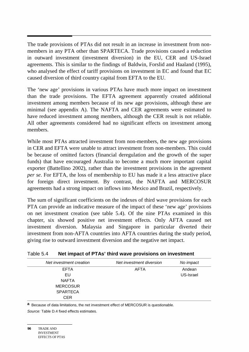
96 TRADE ANDINVESTMENTEFFECTS OF PTAS
The trade provisions of PTAs did not result in an increase in investment from non-members in any PTA other than SPARTECA. Trade provisions caused a reductionin outward investment (investment diversion) in the EU, CER and US-Israelagreements. This is similar to the findings of Baldwin, Forslid and Haaland (1995),who analysed the effect of tariff provisions on investment in EC and found that ECcaused diversion of third country capital from EFTA to the EU.
The ‘new age’ provisions in various PTAs have much more impact on investmentthan the trade provisions. The EFTA agreement apparently created additionalinvestment among members because of its new age provisions, although these areminimal (see appendix A). The NAFTA and CER agreements were estimated tohave reduced investment among members, although the CER result is not reliable.All other agreements considered had no significant effects on investment amongmembers.
While most PTAs attracted investment from non-members, the new age provisionsin CER and EFTA were unable to attract investment from non-members. This couldbe because of omitted factors (financial deregulation and the growth of the superfunds) that have encouraged Australia to become a much more important capitalexporter (Battellino 2002), rather than the investment provisions in the agreementper se. For EFTA, the loss of membership to EU has made it a less attractive placefor foreign direct investment. By contrast, the NAFTA and MERCOSURagreements had a strong impact on inflows into Mexico and Brazil, respectively.
The sum of significant coefficients on the indexes of third wave provisions for eachPTA can provide an indicative measure of the impact of these ‘new age’ provisionson net investment creation (see table 5.4). Of the nine PTAs examined in thischapter, six showed positive net investment effects. Only AFTA caused netinvestment diversion. Malaysia and Singapore in particular diverted theirinvestment from non-AFTA countries into AFTA countries during the study period,giving rise to outward investment diversion and the negative net impact.
Table 5.4 Net impact of PTAs’ third wave provisions on investment
Net investment creation Net investment diversion No impact
EFTAEU
NAFTAMERCOSURSPARTECA
CER
AFTA AndeanUS-Israel
a Because of data limitations, the net investment effect of MERCOSUR is questionable.
Source: Table D.4 fixed effects estimates.
INVESTMENTCREATION ANDDIVERSION
97
NAFTA, EU, CER and to a lesser extent EFTA caused net investment creation, notbecause they stimulated investment among members, but because they appear tohave stimulated outward investment from member to non-member countries. This isconsistent with these regions being major sources of FDI, but suggests that theestimated effects may well reflect the influence of causal factors not controlled forin the analysis that make these countries net capital exporters, rather than the effectsof PTA formation/expansion per se.
The Andean and US-Israel agreements had no significant impact on net investmentcreation.
Though the investment results appear to be more positive than the results reportedfor trade in chapter 4, there are number of qualifications that need to be considered.Winters (1997) argued that new FDI from any source could go into the productionof goods for trade diversion and thus worsen the PTA’s welfare overall. In a similarvein, McLaren (2002) argued that
A regional trade regime can plausibly be interpreted as a coordination failure, in whichthe anticipation that the world will break into regional trade blocs induces sunk privatesector investments that then lead to a demand for regionalism. Under this argument,regionalism can be Pareto-worsening even though once sunk investments have beenmade it is, ex post, a relatively efficient compromise: hence, regionalism is ‘insidious’,the damage it does to efficiency is hidden in the distortion of ex ante investments(McLaren 2002, p. 572)
The gravity model estimates provide indications of the positive net investmenteffects of PTAs, but do not consider whether the resulting investment contributes totrade diversion.
Further, as noted before, a finding of net investment creation is a weak indicator ofwhether the welfare gains from investment creation outweigh the welfare costs ofinvestment diversion. Investment diversion may dominate creation in welfare terms,even if it does not in ‘volume of investment’ terms. On the other hand, if the non-trade provisions reduce restrictions that raise costs, then member countries can gainin welfare terms, despite investment diversion. But in either case, members couldwell gain even more from multilateral liberalisation of non-trade restrictions.
5.4 Summary
It is possible for PTAs to have more adverse effects on investment flows than tradeflows. Investment could be diverted into a PTA to take advantage of its tradeprovisions, and the trade carried out from those beachheads could constitutetraditional trade diversion.
98 TRADE ANDINVESTMENTEFFECTS OF PTAS
However, the present analysis finds little evidence of such beachhead investment.Instead, it finds evidence of net investment creation in response to the ‘new age’non-trade provisions of PTAs. Thus the finding on investment is more positive thanfor trade, but not without qualifications.
The welfare consequences of these findings are discussed in the next chapter.
SUMMING UP 99
6 Summing up
Previous chapters have examined, both theoretically and empirically, the likelyeffects of the trade and non-trade provisions of PTAs on the trade and foreign directinvestment flows of members and non-members. They have also highlighted theimplications for the economic welfare of members and non-members. This chapterdraws on these findings to reach some tentative conclusions about the effects ofpreferential trade agreements.
6.1 Trade provisions
Contrary to popular conception, the main benefits to a country from preferential (orany) trade arrangements come, not from export opportunities (since these costdomestic resources), but from their ability to provide import needs at lower realresource cost. This is ultimately what can improve a country’s living standards.
Both theoretical and empirical work has highlighted that PTAs can boost tradeamong members, but this is often at the expense of non-members. So whether it isbeneficial overall to join a PTA depends on the cost structures in partner countries,compared with the cost structures in third parties. If a preferential trade arrangementdiverts a country’s imports from a low-cost third party to a higher-cost preferentialtrade partner, it can be made worse off. Thus, the best chance a country has to gainfrom preferential trading arrangements would be to choose a trading partner withthe lowest (quality-adjusted) costs. But then the economic rationale for liberalisingpreferentially, rather than unilaterally across-the-board, is lost.
The theoretical literature reviewed in this paper has always noted the possibility oflosses from net trade diversion, and the empirical work undertaken here suggeststhat this trade outcome is more common than other recent empirical analyses havesuggested. The hypothetical (often computable general equilibrium) analyses ofPTAs have sometimes made assumptions that have skewed the findings in favour ofeconomically beneficial outcomes. They typically also model very pure and stylisedarrangements — not the complex, selective, and overlapping arrangements thatapply in practice. And the econometric exercises examining the effects of actualPTAs on actual trade flows have often not been sufficiently careful in the way theyhave characterised the coverage of the PTA provisions. Nor have they tested
100 TRADE ANDINVESTMENTEFFECTS OF PTAS
rigorously whether the trade effects of PTAs were any stronger after PTAimplementation than before.
The empirical work in chapter 4 suggests that of the 18 recent PTAs examined indetail, 12 have diverted more trade from non-members than they have createdamong members. What is more, some of the apparently quite liberal PTAs —including EU, NAFTA and MERCOSUR — have failed to create significantadditional trade among members (relative to the average trade patterns amongcountries in the sample).
Part of the reason for this negative finding is the more rigorous statistical test thathas been applied here to test whether intra-bloc trade is significantly greater afterbloc formation (or expansion) than before. In the past, this was assessed, at best,only by reference to the point estimates from various cross sections. But the findingis also consistent with the fact that many of the provisions needed in preferentialarrangements to underpin and enforce their preferential nature — such as rules oforigin — are in practice quite trade restricting.
A country could nevertheless gain individually from a preferential tradingarrangement, even if the arrangement failed to create significant net trade overall.The gain could come if the terms of trade turned in its favour as a result of the PTA.But the very same phenomenon could threaten any gains to the partner country,further inducing them to seek exclusions for sensitive high-tariff sectors.
6.2 Non-trade provisions
The distinguishing characteristic of recent, third-wave PTAs is that they cover muchmore than just merchandise trade. Investment, services, competition policy,government procurement, e-commerce, labour and environmental standards are alsoincreasingly on the agenda.
While the increasing focus of PTAs on non-trade provisions may suggest thatconventional concerns about trade diversion are outmoded, some theoreticalliterature suggests this conclusion is premature.
On the one hand, in an increasingly integrated world economy, even minor tradeconcessions can have a significant impact on investment flows. And if investment isattracted into one PTA partner in order to serve the markets of the others, then thetrade from such beachhead positions can constitute traditional trade diversion.
On the other, the non-trade provisions of PTAs, particularly those related toinvestment and services, can also have a significant impact on investment flows. But
SUMMING UP 101
the preferential nature of the PTA provisions may mean that investment is divertedfrom a low-cost to a higher-cost host country, and such investment diversion canalso be harmful.
The analysis in chapter 5 is among the first to check these propositions empirically.It finds little evidence of beachhead investment, or an unwinding of ‘tariff-jumping’investment, in response to the trade provisions of PTAs. Only for SPARTECA andthe US-Israel agreement, for example, is there (weak) evidence of foreign directinvestment responding in beachhead fashion to trade provisions. And the result forUS-Israel is further qualified by the imprecision of the intra-bloc effect with justtwo countries involved.
Chapter 5 does find evidence that foreign direct investment responds significantly tothe non-trade provisions of PTAs. Interestingly, this is in contrast to a lack ofresponse of FDI to bilateral investment treaties.
Further, for most of those agreements where non-trade provisions have affectedFDI, the result has been net investment creation rather than diversion.
Although it is a weak test, this suggests that on balance, the non-trade provisions ofthese PTAs have created an efficient geographic distribution of FDI. This isconsistent with the fact that at least some of the non-trade provisions (egcommitments to more strongly enforce intellectual property rights) are not stronglypreferential in their nature.
Further, the theoretical literature has stressed that if the non-trade barriers are of thesort to raise the real resource costs of doing business, rather than simply to createrents that raise prices above costs, then preferential liberalisation will be beneficial,even in the absence of net investment creation.
However, the trade that may be generated from the new FDI positions may still bediverted in the ‘wrong’ direction in response to the trade provisions of PTAs, andmay therefore contribute to the net trade diversion found in chapter 4.
Thus the results of this research suggest that there may be real economic gains fromthe non-trade provisions of third-wave PTAs, but they also suggest that there arestill economic costs associated with the preferential nature of the trade provisions.And these costs could be magnified in a world of increasing capital mobility.
Thus the findings of this research on the effects of the non-trade provisions of PTAsare more positive than those on the trade provisions. This suggests there could bereal benefits if countries could use regional negotiations to persuade trading partnersto make progress in reforming such things as investment, services, competition

102 TRADE ANDINVESTMENTEFFECTS OF PTAS
policy and government procurement, especially if this is done on a non-preferentialbasis.
MEMBERLIBERALISATIONINDEX
103
A Member Liberalisation Index
This appendix outlines the methodology used in constructing the MemberLiberalisation Index (MLI) and the results obtained from this index. The indexmethodology gives a measure of the breadth and depth of the coverage of PTAs. Inessence, the index shows the extent to which trade and investment conditionsbetween members have been liberalised, allowing a comparison of differentarrangements and their provisions. The index was calculated for a selection ofdifferent PTAs and the results from the index are used to characterise each of thesePTAs in the empirical analysis.
A.1 Methodology
The member liberalisation index (MLI) assesses arrangements that govern trade andinvestment among PTA members. It does not compare this to the arrangements thatgovern trade between members and non-members. Hence it does not measure themargin of preference created by the PTA. Table A.1 at the end of this appendixdescribes the MLI in detail.
A number of agreements were assessed using the MLI. They were generallyselected on the basis of whether:
• Australia is a member — CER, SPARTECA and PATCRA;
• Australia is not a member, but the agreement is likely to affect the trade flows ofAustralia’s major trading partners — NAFTA, ASEAN and the EU; or
• they are representative of a cross-section of bilateral agreements — Chile-Mexico, EU-Poland and Singapore-New Zealand.
The texts of the agreements were obtained from a variety of sources, including theOrganization of American States (OAS 2002), the European Union On-line (EU2001) and the World Trade Organisation (WTO 2001).
Classifying provisions in PTAs
The provisions in PTAs are first classified according to the type of trade that iscovered:
104 TRADE ANDINVESTMENTEFFECTS OF PTAS
• agricultural goods, with provisions covering such things as domestic supportmeasures and export incentives;
• industrial goods, with provisions covering such things as rules of origin andtariff reduction schedules;
• services, with provisions covering services generally; and
• all trade, with provisions covering such things as domestic competition policy,intellectual property rights and the movement of people.
The weights given to the first three broad categories have been chosen to reflectvery roughly their relative importance in total world trade.1 Where provisions affecttrade in more than one grouping, they are included twice in the index. For example,rules of origin are relevant for both agricultural and industrial goods.
Calculating the index
Different categories of provisions are collected under each of the four majorgroupings, and the overall weight assigned to the grouping is divided among thecategories. Then, within each category, a set of criteria is used to judge eachprovision based on the extent to which it progresses liberalisation among members.
The relative weights given to each category are based on a judgement of their likelyrelative impact on trade. For example, the category for antidumping andcountervailing is judged to have a larger impact on trade in industrial products andis given a weight of 0.08. On the other hand, the category for the number ofdifferent types of rules of origin is judged to have a smaller impact on trade and isgiven a weight of 0.03.
The provisions in PTAs are assessed against a set of criteria for each category. Thecriteria range from least liberal to most liberal and the greater the liberalisation,greater the score. The scores range from 0 (least liberal) to 1 (most liberal). Forexample, the investment category is assessed according to the following criteria —no provisions (least liberal), initiatives to reduce restrictions and facilitateinvestment, provisions giving national treatment for investors and provisions thatprohibit restrictions on investment (most liberal).
The score for ‘no provision’ is assigned where the PTA has no provisions relating tothat area of trade. This score depends on whether the provisions in that categoryusually promote or inhibit trade. Categories that aim to promote trade (eg
1 The weight for services trade will be understated because available statistics exclude commercial
presence as mode of supply (Hardin and Holmes 1997).
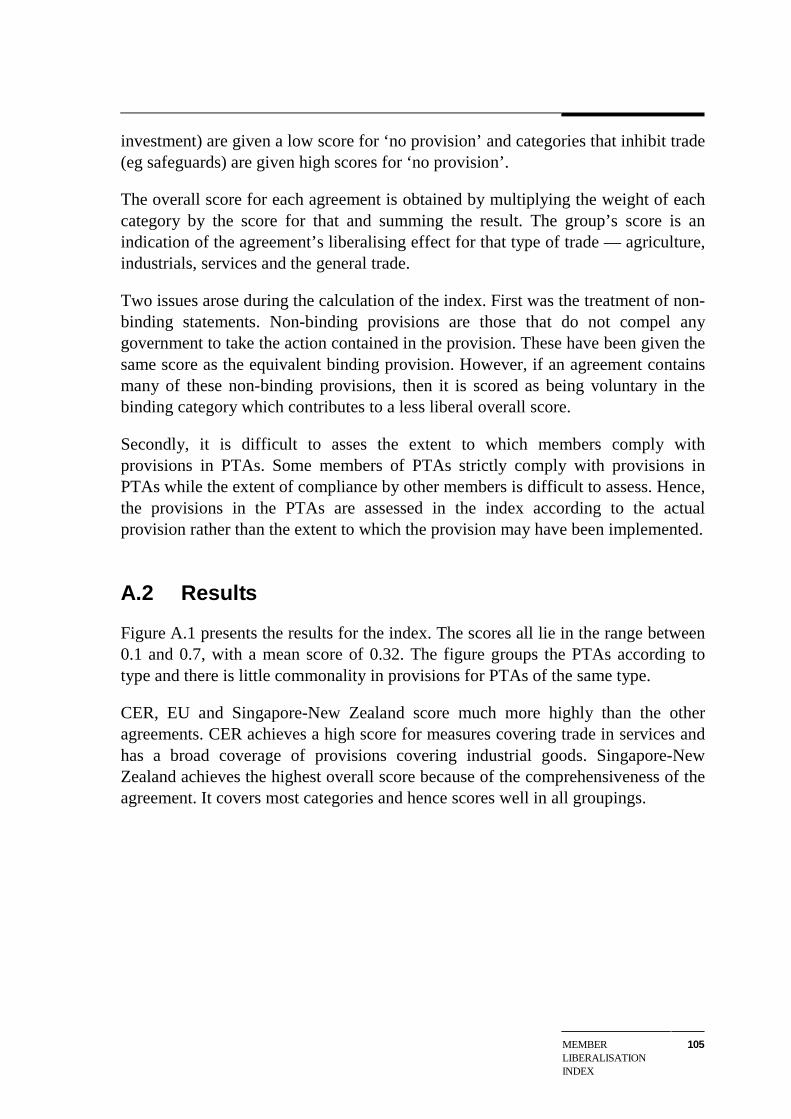
MEMBERLIBERALISATIONINDEX
105
investment) are given a low score for ‘no provision’ and categories that inhibit trade(eg safeguards) are given high scores for ‘no provision’.
The overall score for each agreement is obtained by multiplying the weight of eachcategory by the score for that and summing the result. The group’s score is anindication of the agreement’s liberalising effect for that type of trade — agriculture,industrials, services and the general trade.
Two issues arose during the calculation of the index. First was the treatment of non-binding statements. Non-binding provisions are those that do not compel anygovernment to take the action contained in the provision. These have been given thesame score as the equivalent binding provision. However, if an agreement containsmany of these non-binding provisions, then it is scored as being voluntary in thebinding category which contributes to a less liberal overall score.
Secondly, it is difficult to asses the extent to which members comply withprovisions in PTAs. Some members of PTAs strictly comply with provisions inPTAs while the extent of compliance by other members is difficult to assess. Hence,the provisions in the PTAs are assessed in the index according to the actualprovision rather than the extent to which the provision may have been implemented.
A.2 Results
Figure A.1 presents the results for the index. The scores all lie in the range between0.1 and 0.7, with a mean score of 0.32. The figure groups the PTAs according totype and there is little commonality in provisions for PTAs of the same type.
CER, EU and Singapore-New Zealand score much more highly than the otheragreements. CER achieves a high score for measures covering trade in services andhas a broad coverage of provisions covering industrial goods. Singapore-NewZealand achieves the highest overall score because of the comprehensiveness of theagreement. It covers most categories and hence scores well in all groupings.
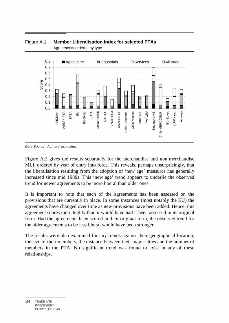
106 TRADE ANDINVESTMENTEFFECTS OF PTAS
Figure A.1 Member Liberalisation Index for selected PTAsAgreements ordered by type
0.0
0.1
0.2
0.3
0.4
0.5
0.6
0.7
0.8A
ND
EA
N
AS
EA
N-F
TA
EF
TA
EU
EU
-Sw
itz
LAIA
ME
RC
OS
UR
NA
FT
A
SP
AR
TE
CA
AN
ZC
ER
TA
Chi
le-C
olom
bia
Chi
le-M
exic
o
Isra
el-U
S
PA
TC
RA
Sin
gapo
re-N
Z
Chi
le-M
ER
CO
SU
R
EU
-Egy
pt
EU
-Pol
and
Ave
rage
Sco
re
Agriculture Industrials Services All trade
Data Source: Authors’ estimates.
Figure A.2 gives the results separately for the merchandise and non-merchandiseMLI, ordered by year of entry into force. This reveals, perhaps unsurprisingly, thatthe liberalisation resulting from the adoption of ‘new age’ measures has generallyincreased since mid 1980s. This ‘new age’ trend appears to underlie the observedtrend for newer agreements to be more liberal than older ones.
It is important to note that each of the agreements has been assessed on theprovisions that are currently in place. In some instances (most notably the EU) theagreements have changed over time as new provisions have been added. Hence, thisagreement scores more highly than it would have had it been assessed in its originalform. Had the agreements been scored in their original form, the observed trend forthe older agreements to be less liberal would have been stronger.
The results were also examined for any trends against their geographical location,the size of their members, the distance between their major cities and the number ofmembers in the PTA. No significant trend was found to exist in any of theserelationships.
MEMBERLIBERALISATIONINDEX
107
Figure A.2 Merchandise and non-merchandise MLIs for selected PTAsAgreements ordered by year of commencement
0.00.10.20.30.40.50.60.70.8
EU
(19
58)
EF
TA
(19
60)
AN
DE
AN
(19
69)
EU
-Sw
itz (
1973
)
PA
TC
RA
(19
77)
EU
-Egy
pt (
1978
)
LAIA
(19
80)
SP
AR
TE
CA
(19
81)
AN
ZC
ER
TA
(19
83)
Isra
el-U
S (
1985
)
AS
EA
N-F
TA
(19
92)
ME
RC
OS
UR
(19
91)
Chi
le-C
olom
bia
(199
3)
NA
FT
A (
1989
/199
3)
EU
-Pol
and
(199
4)
Chi
le-M
ER
CO
SU
R (
1996
)
Chi
le-M
exic
o (1
999)
Sin
gapo
re-N
Z (
2000
)
Sco
re
Merchandise trade Non-merchandise trade
Data Source: Authors’ estimates.
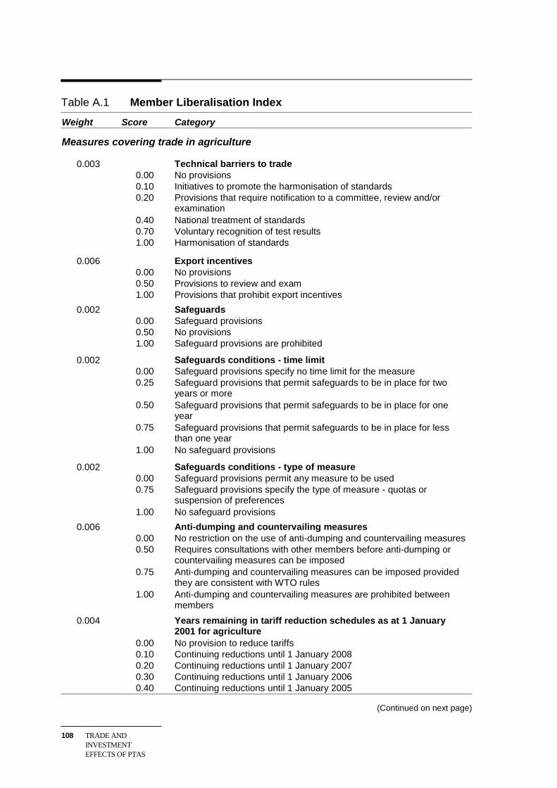
108 TRADE ANDINVESTMENTEFFECTS OF PTAS
Table A.1 Member Liberalisation Index
Weight Score Category
Measures covering trade in agriculture
0.003 Technical barriers to trade0.00 No provisions0.10 Initiatives to promote the harmonisation of standards0.20 Provisions that require notification to a committee, review and/or
examination0.40 National treatment of standards0.70 Voluntary recognition of test results1.00 Harmonisation of standards
0.006 Export incentives0.00 No provisions0.50 Provisions to review and exam1.00 Provisions that prohibit export incentives
0.002 Safeguards0.00 Safeguard provisions0.50 No provisions1.00 Safeguard provisions are prohibited
0.002 Safeguards conditions - time limit0.00 Safeguard provisions specify no time limit for the measure0.25 Safeguard provisions that permit safeguards to be in place for two
years or more0.50 Safeguard provisions that permit safeguards to be in place for one
year0.75 Safeguard provisions that permit safeguards to be in place for less
than one year1.00 No safeguard provisions
0.002 Safeguards conditions - type of measure0.00 Safeguard provisions permit any measure to be used0.75 Safeguard provisions specify the type of measure - quotas or
suspension of preferences1.00 No safeguard provisions
0.006 Anti-dumping and countervailing measures0.00 No restriction on the use of anti-dumping and countervailing measures0.50 Requires consultations with other members before anti-dumping or
countervailing measures can be imposed0.75 Anti-dumping and countervailing measures can be imposed provided
they are consistent with WTO rules1.00 Anti-dumping and countervailing measures are prohibited between
members
0.004 Years remaining in tariff reduction schedules as at 1 January2001 for agriculture
0.00 No provision to reduce tariffs0.10 Continuing reductions until 1 January 20080.20 Continuing reductions until 1 January 20070.30 Continuing reductions until 1 January 20060.40 Continuing reductions until 1 January 2005
(Continued on next page)
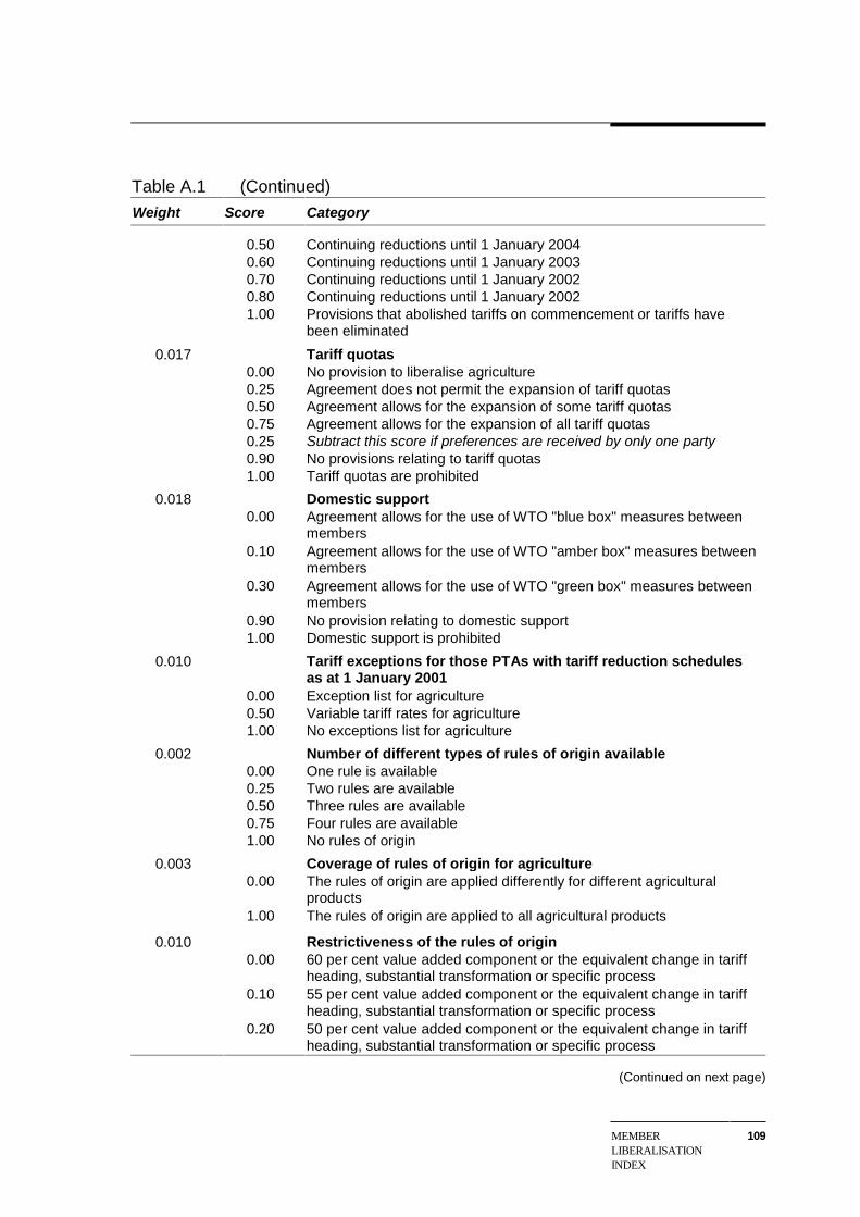
MEMBERLIBERALISATIONINDEX
109
Table A.1 (Continued)
Weight Score Category
0.50 Continuing reductions until 1 January 20040.60 Continuing reductions until 1 January 20030.70 Continuing reductions until 1 January 20020.80 Continuing reductions until 1 January 20021.00 Provisions that abolished tariffs on commencement or tariffs have
been eliminated
0.017 Tariff quotas0.00 No provision to liberalise agriculture0.25 Agreement does not permit the expansion of tariff quotas0.50 Agreement allows for the expansion of some tariff quotas0.75 Agreement allows for the expansion of all tariff quotas0.25 Subtract this score if preferences are received by only one party0.90 No provisions relating to tariff quotas1.00 Tariff quotas are prohibited
0.018 Domestic support0.00 Agreement allows for the use of WTO "blue box" measures between
members0.10 Agreement allows for the use of WTO "amber box" measures between
members0.30 Agreement allows for the use of WTO "green box" measures between
members0.90 No provision relating to domestic support1.00 Domestic support is prohibited
0.010 Tariff exceptions for those PTAs with tariff reduction schedulesas at 1 January 2001
0.00 Exception list for agriculture0.50 Variable tariff rates for agriculture1.00 No exceptions list for agriculture
0.002 Number of different types of rules of origin available0.00 One rule is available0.25 Two rules are available0.50 Three rules are available0.75 Four rules are available1.00 No rules of origin
0.003 Coverage of rules of origin for agriculture0.00 The rules of origin are applied differently for different agricultural
products1.00 The rules of origin are applied to all agricultural products
0.010 Restrictiveness of the rules of origin0.00 60 per cent value added component or the equivalent change in tariff
heading, substantial transformation or specific process0.10 55 per cent value added component or the equivalent change in tariff
heading, substantial transformation or specific process0.20 50 per cent value added component or the equivalent change in tariff
heading, substantial transformation or specific process
(Continued on next page)
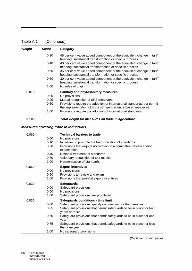
110 TRADE ANDINVESTMENTEFFECTS OF PTAS
Table A.1 (Continued)
Weight Score Category
0.30 45 per cent value added component or the equivalent change in tariffheading, substantial transformation or specific process
0.40 40 per cent value added component or the equivalent change in tariffheading, substantial transformation or specific process
0.50 35 per cent value added component or the equivalent change in tariffheading, substantial transformation or specific process
0.60 30 per cent value added component or the equivalent change in tariffheading, substantial transformation or specific process
1.00 No rules of origin
0.015 Sanitary and phytosanitary measures0.00 No provisions0.25 Mutual recognition of SPS measures0.50 Provisions require the adoption of international standards, but permit
the implementation of more stringent science-based measures1.00 Provisions require the adoption of international standards
0.100 Total weight for measures on trade in agriculture
Measures covering trade in industrials
0.060 Technical barriers to trade0.00 No provisions0.10 Initiatives to promote the harmonisation of standards0.20 Provisions that require notification to a committee, review and/or
examination0.40 National treatment of standards0.70 Voluntary recognition of test results1.00 Harmonisation of standards
0.060 Export incentives0.00 No provisions0.50 Provisions to review and exam1.00 Provisions that prohibit export incentives
0.030 Safeguards0.00 Safeguard provisions0.50 No provisions1.00 Safeguard provisions are prohibited
0.030 Safeguards conditions - time limit0.00 Safeguard provisions specify no time limit for the measure0.25 Safeguard provisions that permit safeguards to be in place for two
years or more0.50 Safeguard provisions that permit safeguards to be in place for one
year0.75 Safeguard provisions that permit safeguards to be in place for less
than one year1.00 No safeguard provisions
(Continued on next page)
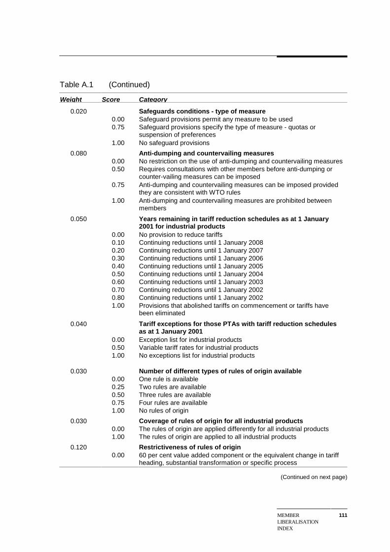
MEMBERLIBERALISATIONINDEX
111
Table A.1 (Continued)
Weight Score Category
0.020 Safeguards conditions - type of measure0.00 Safeguard provisions permit any measure to be used0.75 Safeguard provisions specify the type of measure - quotas or
suspension of preferences1.00 No safeguard provisions
0.080 Anti-dumping and countervailing measures0.00 No restriction on the use of anti-dumping and countervailing measures0.50 Requires consultations with other members before anti-dumping or
counter-vailing measures can be imposed0.75 Anti-dumping and countervailing measures can be imposed provided
they are consistent with WTO rules1.00 Anti-dumping and countervailing measures are prohibited between
members
0.050 Years remaining in tariff reduction schedules as at 1 January2001 for industrial products
0.00 No provision to reduce tariffs0.10 Continuing reductions until 1 January 20080.20 Continuing reductions until 1 January 20070.30 Continuing reductions until 1 January 20060.40 Continuing reductions until 1 January 20050.50 Continuing reductions until 1 January 20040.60 Continuing reductions until 1 January 20030.70 Continuing reductions until 1 January 20020.80 Continuing reductions until 1 January 20021.00 Provisions that abolished tariffs on commencement or tariffs have
been eliminated
0.040 Tariff exceptions for those PTAs with tariff reduction schedulesas at 1 January 2001
0.00 Exception list for industrial products0.50 Variable tariff rates for industrial products1.00 No exceptions list for industrial products
0.030 Number of different types of rules of origin available0.00 One rule is available0.25 Two rules are available0.50 Three rules are available0.75 Four rules are available1.00 No rules of origin
0.030 Coverage of rules of origin for all industrial products0.00 The rules of origin are applied differently for all industrial products1.00 The rules of origin are applied to all industrial products
0.120 Restrictiveness of rules of origin0.00 60 per cent value added component or the equivalent change in tariff
heading, substantial transformation or specific process
(Continued on next page)
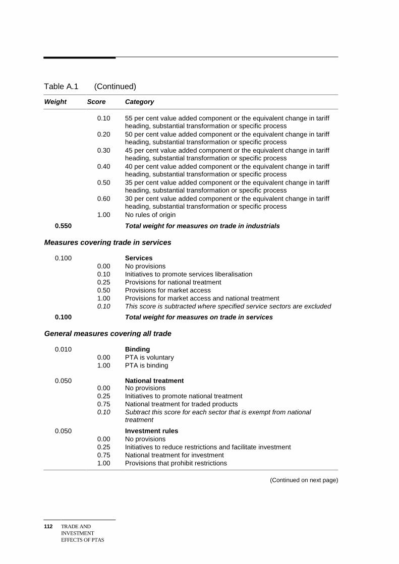
112 TRADE ANDINVESTMENTEFFECTS OF PTAS
Table A.1 (Continued)
Weight Score Category
0.10 55 per cent value added component or the equivalent change in tariffheading, substantial transformation or specific process
0.20 50 per cent value added component or the equivalent change in tariffheading, substantial transformation or specific process
0.30 45 per cent value added component or the equivalent change in tariffheading, substantial transformation or specific process
0.40 40 per cent value added component or the equivalent change in tariffheading, substantial transformation or specific process
0.50 35 per cent value added component or the equivalent change in tariffheading, substantial transformation or specific process
0.60 30 per cent value added component or the equivalent change in tariffheading, substantial transformation or specific process
1.00 No rules of origin
0.550 Total weight for measures on trade in industrials
Measures covering trade in services
0.100 Services0.00 No provisions0.10 Initiatives to promote services liberalisation0.25 Provisions for national treatment0.50 Provisions for market access1.00 Provisions for market access and national treatment0.10 This score is subtracted where specified service sectors are excluded
0.100 Total weight for measures on trade in services
General measures covering all trade
0.010 Binding0.00 PTA is voluntary1.00 PTA is binding
0.050 National treatment0.00 No provisions0.25 Initiatives to promote national treatment0.75 National treatment for traded products0.10 Subtract this score for each sector that is exempt from national
treatment
0.050 Investment rules0.00 No provisions0.25 Initiatives to reduce restrictions and facilitate investment0.75 National treatment for investment1.00 Provisions that prohibit restrictions
(Continued on next page)
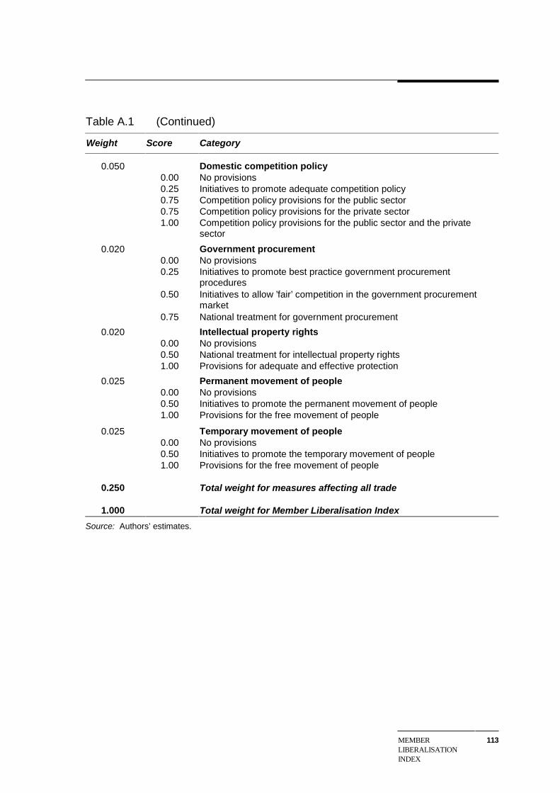
MEMBERLIBERALISATIONINDEX
113
Table A.1 (Continued)
Weight Score Category
0.050 Domestic competition policy0.00 No provisions0.25 Initiatives to promote adequate competition policy0.75 Competition policy provisions for the public sector0.75 Competition policy provisions for the private sector1.00 Competition policy provisions for the public sector and the private
sector
0.020 Government procurement0.00 No provisions0.25 Initiatives to promote best practice government procurement
procedures0.50 Initiatives to allow ’fair’ competition in the government procurement
market0.75 National treatment for government procurement
0.020 Intellectual property rights0.00 No provisions0.50 National treatment for intellectual property rights1.00 Provisions for adequate and effective protection
0.025 Permanent movement of people0.00 No provisions0.50 Initiatives to promote the permanent movement of people1.00 Provisions for the free movement of people
0.025 Temporary movement of people0.00 No provisions0.50 Initiatives to promote the temporary movement of people1.00 Provisions for the free movement of people
0.250 Total weight for measures affecting all trade
1.000 Total weight for Member Liberalisation Index
Source: Authors’ estimates.
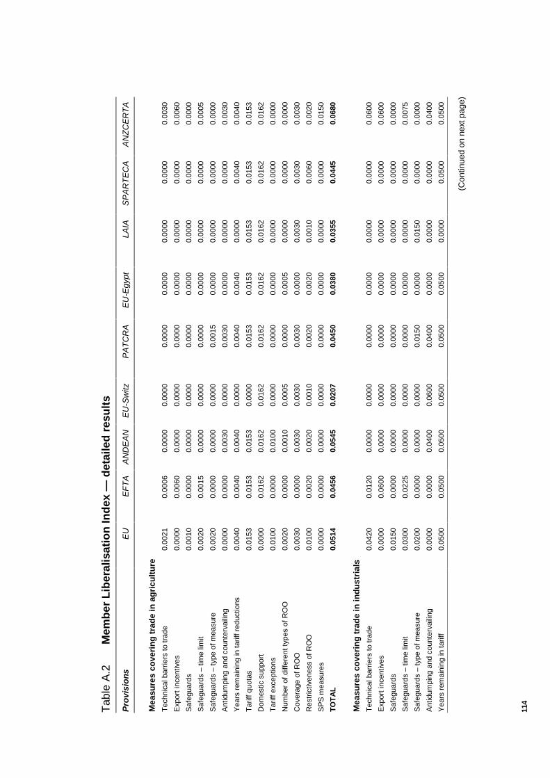
114
Tab
le A
.2M
emb
er L
iber
alis
atio
n In
dex
— d
etai
led
res
ult
s
Pro
visi
on
sE
UE
FT
AA
ND
EA
NE
U-S
witz
PA
TC
RA
EU
-Egy
ptLA
IAS
PA
RT
EC
AA
NZ
CE
RT
A
Mea
sure
s co
veri
ng
tra
de
in a
gri
cult
ure
Tec
hnic
al b
arrie
rs to
trad
e0.
0021
0.00
060.
0000
0.00
000.
0000
0.00
000.
0000
0.00
000.
0030
Exp
ort i
ncen
tives
0.00
000.
0060
0.00
000.
0000
0.00
000.
0000
0.00
000.
0000
0.00
60
Saf
egua
rds
0.00
100.
0000
0.00
000.
0000
0.00
000.
0000
0.00
000.
0000
0.00
00
Saf
egua
rds
– tim
e lim
it0.
0020
0.00
150.
0000
0.00
000.
0000
0.00
000.
0000
0.00
000.
0005
Saf
egua
rds
– ty
pe o
f mea
sure
0.00
200.
0000
0.00
000.
0000
0.00
150.
0000
0.00
000.
0000
0.00
00
Ant
idum
ping
and
cou
nter
vaili
ng0.
0000
0.00
000.
0030
0.00
000.
0030
0.00
000.
0000
0.00
000.
0030
Yea
rs r
emai
ning
in ta
riff r
educ
tions
0.00
400.
0040
0.00
400.
0000
0.00
400.
0040
0.00
000.
0040
0.00
40
Tar
iff q
uota
s0.
0153
0.01
530.
0153
0.00
000.
0153
0.01
530.
0153
0.01
530.
0153
Dom
estic
sup
port
0.00
000.
0162
0.01
620.
0162
0.01
620.
0162
0.01
620.
0162
0.01
62
Tar
iff e
xcep
tions
0.01
000.
0000
0.01
000.
0000
0.00
000.
0000
0.00
000.
0000
0.00
00
Num
ber
of d
iffer
ent t
ypes
of R
OO
0.00
200.
0000
0.00
100.
0005
0.00
000.
0005
0.00
000.
0000
0.00
00
Cov
erag
e of
RO
O0.
0030
0.00
000.
0030
0.00
300.
0030
0.00
000.
0030
0.00
300.
0030
Res
tric
tiven
ess
of R
OO
0.01
000.
0020
0.00
200.
0010
0.00
200.
0020
0.00
100.
0060
0.00
20
SP
S m
easu
res
0.00
000.
0000
0.00
000.
0000
0.00
000.
0000
0.00
000.
0000
0.01
50
TO
TA
L0.
0514
0.04
560.
0545
0.02
070.
0450
0.03
800.
0355
0.04
450.
0680
Mea
sure
s co
veri
ng
tra
de
in in
du
stri
als
Tec
hnic
al b
arrie
rs to
trad
e0.
0420
0.01
200.
0000
0.00
000.
0000
0.00
000.
0000
0.00
000.
0600
Exp
ort i
ncen
tives
0.00
000.
0600
0.00
000.
0000
0.00
000.
0000
0.00
000.
0000
0.06
00
Saf
egua
rds
0.01
500.
0000
0.00
000.
0000
0.00
000.
0000
0.00
000.
0000
0.00
00
Saf
egua
rds
– tim
e lim
it0.
0300
0.02
250.
0000
0.00
000.
0000
0.00
000.
0000
0.00
000.
0075
Saf
egua
rds
– ty
pe o
f mea
sure
0.02
000.
0000
0.00
000.
0000
0.01
500.
0000
0.01
500.
0000
0.00
00
Ant
idum
ping
and
cou
nter
vaili
ng0.
0000
0.00
000.
0400
0.06
000.
0400
0.00
000.
0000
0.00
000.
0400
Yea
rs r
emai
ning
in ta
riff
0.05
000.
0500
0.05
000.
0500
0.05
000.
0500
0.00
000.
0500
0.05
00
(Con
tinue
d on
nex
t pag
e)
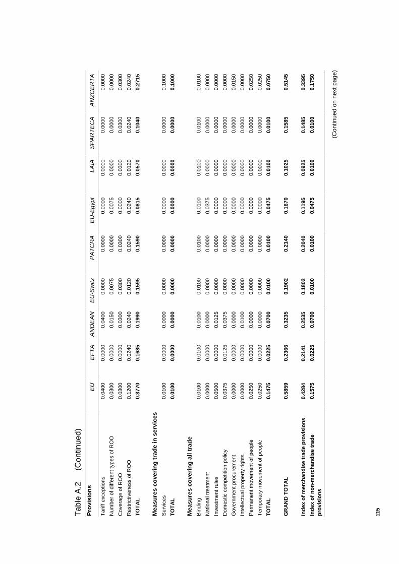
115
Tab
le A
.2
(C
ontin
ued)
Pro
visi
on
sE
UE
FT
AA
ND
EA
NE
U-S
witz
PA
TC
RA
EU
-Egy
ptLA
IAS
PA
RT
EC
AA
NZ
CE
RT
A
Tar
iff e
xcep
tions
0.04
000.
0000
0.04
000.
0000
0.00
000.
0000
0.00
000.
0000
0.00
00
Num
ber
of d
iffer
ent t
ypes
of R
OO
0.03
000.
0000
0.01
500.
0075
0.00
000.
0075
0.00
000.
0000
0.00
00
Cov
erag
e of
RO
O0.
0300
0.00
000.
0300
0.03
000.
0300
0.00
000.
0300
0.03
000.
0300
Res
tric
tiven
ess
of R
OO
0.12
000.
0240
0.02
400.
0120
0.02
400.
0240
0.01
200.
0240
0.02
40
TO
TA
L0.
3770
0.16
850.
1990
0.15
950.
1590
0.08
150.
0570
0.10
400.
2715
Mea
sure
s co
veri
ng
tra
de
in s
ervi
ces
Ser
vice
s0.
0100
0.00
000.
0000
0.00
000.
0000
0.00
000.
0000
0.00
000.
1000
TO
TA
L0.
0100
0.00
000.
0000
0.00
000.
0000
0.00
000.
0000
0.00
000.
1000
Mea
sure
s co
veri
ng
all
trad
eB
indi
ng0.
0100
0.01
000.
0100
0.01
000.
0100
0.01
000.
0100
0.01
000.
0100
Nat
iona
l tre
atm
ent
0.00
000.
0000
0.00
000.
0000
0.00
000.
0375
0.00
000.
0000
0.00
00
Inve
stm
ent r
ules
0.05
000.
0000
0.01
250.
0000
0.00
000.
0000
0.00
000.
0000
0.00
00
Dom
estic
com
petit
ion
polic
y0.
0375
0.01
250.
0375
0.00
000.
0000
0.00
000.
0000
0.00
000.
0000
Gov
ernm
ent p
rocu
rem
ent
0.00
000.
0000
0.00
000.
0000
0.00
000.
0000
0.00
000.
0000
0.01
50
Inte
llect
ual p
rope
rty
right
s0.
0000
0.00
000.
0100
0.00
000.
0000
0.00
000.
0000
0.00
000.
0000
Per
man
ent m
ovem
ent o
f peo
ple
0.02
500.
0000
0.00
000.
0000
0.00
000.
0000
0.00
000.
0000
0.02
50
Tem
pora
ry m
ovem
ent o
f peo
ple
0.02
500.
0000
0.00
000.
0000
0.00
000.
0000
0.00
000.
0000
0.02
50
TO
TA
L0.
1475
0.02
250.
0700
0.01
000.
0100
0.04
750.
0100
0.01
000.
0750
GR
AN
D T
OT
AL
0.58
590.
2366
0.32
350.
1902
0.21
400.
1670
0.10
250.
1585
0.51
45
Ind
ex o
f m
erch
and
ise
trad
e p
rovi
sio
ns
0.42
840.
2141
0.25
350.
1802
0.20
400.
1195
0.09
250.
1485
0.33
95
Ind
ex o
f n
on
-mer
chan
dis
e tr
ade
pro
visi
on
s0.
1575
0.02
250.
0700
0.01
000.
0100
0.04
750.
0100
0.01
000.
1750
(Con
tinue
d on
nex
t pag
e)
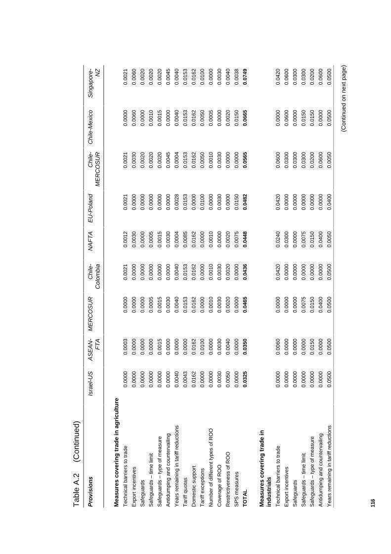
116
Tab
le A
.2
(C
ontin
ued)
Pro
visi
on
sIs
rael
-US
AS
EA
N-
FT
AM
ER
CO
SU
RC
hile
-C
olom
bia
NA
FT
AE
U-P
olan
dC
hile
-M
ER
CO
SU
RC
hile
-Mex
ico
Sin
gapo
re-
NZ
Mea
sure
s co
veri
ng
tra
de
in a
gri
cult
ure
Tec
hnic
al b
arrie
rs to
trad
e0.
0000
0.00
030.
0000
0.00
210.
0012
0.00
210.
0021
0.00
000.
0021
Exp
ort i
ncen
tives
0.00
000.
0000
0.00
000.
0000
0.00
300.
0000
0.00
300.
0060
0.00
60
Saf
egua
rds
0.00
000.
0000
0.00
000.
0000
0.00
000.
0000
0.00
200.
0000
0.00
20
Saf
egua
rds
– tim
e lim
it0.
0000
0.00
000.
0005
0.00
000.
0005
0.00
000.
0020
0.00
100.
0020
Saf
egua
rds
– ty
pe o
f mea
sure
0.00
000.
0015
0.00
150.
0000
0.00
150.
0000
0.00
200.
0015
0.00
20
Ant
idum
ping
and
cou
nter
vaili
ng0.
0000
0.00
000.
0030
0.00
000.
0030
0.00
000.
0045
0.00
000.
0045
Yea
rs r
emai
ning
in ta
riff r
educ
tions
0.00
400.
0000
0.00
400.
0040
0.00
040.
0028
0.00
040.
0040
0.00
40
Tar
iff q
uota
s0.
0043
0.00
000.
0153
0.01
530.
0085
0.01
530.
0153
0.01
530.
0153
Dom
estic
sup
port
0.01
620.
0162
0.01
620.
0162
0.01
620.
0000
0.01
620.
0162
0.01
62
Tar
iff e
xcep
tions
0.00
000.
0100
0.00
000.
0000
0.00
000.
0100
0.00
500.
0050
0.01
00
Num
ber
of d
iffer
ent t
ypes
of R
OO
0.00
000.
0000
0.00
100.
0010
0.00
100.
0000
0.00
100.
0005
0.00
00
Cov
erag
e of
RO
O0.
0030
0.00
300.
0030
0.00
300.
0000
0.00
300.
0030
0.00
000.
0030
Res
tric
tiven
ess
of R
OO
0.00
500.
0040
0.00
200.
0020
0.00
200.
0000
0.00
000.
0020
0.00
40
SP
S m
easu
res
0.00
000.
0000
0.00
000.
0000
0.00
750.
0150
0.00
000.
0150
0.00
38
TO
TA
L0.
0325
0.03
500.
0465
0.04
360.
0448
0.04
820.
0565
0.06
650.
0749
Mea
sure
s co
veri
ng
tra
de
inin
du
stri
als
Tec
hnic
al b
arrie
rs to
trad
e0.
0000
0.00
600.
0000
0.04
200.
0240
0.04
200.
0600
0.00
000.
0420
Exp
ort i
ncen
tives
0.00
000.
0000
0.00
000.
0000
0.03
000.
0000
0.03
000.
0600
0.06
00
Saf
egua
rds
0.00
000.
0000
0.00
000.
0000
0.00
000.
0000
0.03
000.
0000
0.03
00
Saf
egua
rds
– tim
e lim
it0.
0000
0.00
000.
0075
0.00
000.
0075
0.00
000.
0300
0.01
500.
0300
Saf
egua
rds
– ty
pe o
f mea
sure
0.00
000.
0150
0.01
500.
0000
0.01
500.
0000
0.02
000.
0150
0.02
00
Ant
idum
ping
and
cou
nter
vaili
ng0.
0000
0.00
000.
0400
0.00
000.
0400
0.00
000.
0600
0.00
000.
0600
Yea
rs r
emai
ning
in ta
riff r
educ
tions
0.05
000.
0500
0.05
000.
0500
0.00
500.
0400
0.00
500.
0500
0.05
00
(Con
tinue
d on
nex
t pag
e)
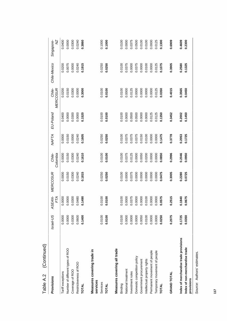
117
Tab
le A
.2
(C
ontin
ued)
Pro
visi
on
sIs
rael
-US
AS
EA
N-
FT
AM
ER
CO
SU
RC
hile
-C
olom
bia
NA
FT
AE
U-P
olan
dC
hile
-M
ER
CO
SU
RC
hile
-Mex
ico
Sin
gapo
re-
NZ
Tar
iff e
xcep
tions
0.00
000.
0000
0.00
000.
0000
0.00
000.
0400
0.02
000.
0200
0.04
00
Num
ber
of d
iffer
ent t
ypes
of R
OO
0.00
000.
0000
0.01
500.
0150
0.01
500.
0000
0.01
500.
0075
0.00
00
Cov
erag
e of
RO
O0.
0300
0.03
000.
0300
0.03
000.
0000
0.03
000.
0300
0.00
000.
0300
Res
tric
tiven
ess
of R
OO
0.06
000.
0480
0.02
400.
0240
0.02
400.
0000
0.00
000.
0240
0.02
40
TO
TA
L0.
1400
0.14
900.
1815
0.16
100.
1605
0.15
200.
3000
0.19
150.
3860
Mea
sure
s co
veri
ng
tra
de
inse
rvic
esS
ervi
ces
0.01
000.
0100
0.02
500.
0100
0.02
500.
0100
0.01
000.
0250
0.10
00
TO
TA
L0.
0100
0.01
000.
0250
0.01
000.
0250
0.01
000.
0100
0.02
500.
1000
Mea
sure
s co
veri
ng
all
trad
e
Bin
ding
0.01
000.
0100
0.01
000.
0100
0.01
000.
0100
0.01
000.
0100
0.01
00
Nat
iona
l tre
atm
ent
0.00
000.
0000
0.00
000.
0375
0.03
750.
0000
0.00
000.
0375
0.00
00
Inve
stm
ent r
ules
0.00
000.
0375
0.03
750.
0125
0.03
750.
0500
0.01
250.
0000
0.03
75
Dom
estic
com
petit
ion
polic
y0.
0000
0.00
000.
0000
0.00
000.
0375
0.05
000.
0000
0.03
750.
0500
Gov
ernm
ent p
rocu
rem
ent
0.00
500.
0000
0.00
000.
0050
0.01
500.
0000
0.00
000.
0000
0.01
00
Inte
llect
ual p
rope
rty
right
s0.
0100
0.01
000.
0000
0.02
000.
0100
0.00
000.
0000
0.01
000.
0100
Per
man
ent m
ovem
ent o
f peo
ple
0.00
000.
0000
0.00
000.
0000
0.00
000.
0125
0.00
000.
0000
0.00
00
Tem
pora
ry m
ovem
ent o
f peo
ple
0.00
000.
0000
0.00
000.
0000
0.00
000.
0125
0.01
250.
0125
0.01
25
TO
TA
L0.
0250
0.05
750.
0475
0.08
500.
1475
0.13
500.
0350
0.10
750.
1300
GR
AN
D T
OT
AL
0.20
750.
2515
0.30
050.
2996
0.37
780.
3452
0.40
150.
3905
0.69
09
Ind
ex o
f m
erch
and
ise
trad
e p
rovi
sio
ns
0.17
250.
1840
0.22
800.
2046
0.20
530.
2002
0.35
650.
2580
0.46
09
Ind
ex o
f n
on
-mer
chan
dis
e tr
ade
pro
visi
on
s0.
0350
0.06
750.
0725
0.09
500.
1725
0.14
500.
0450
0.13
250.
2300
Sou
rce:
Aut
hors
’ est
imat
es.

118 TRADE ANDINVESTMENTEFFECTS OF PTAS
DATA SOURCES 119
B Data sources
B.1 Dependent variables
This study used data on bilateral trade and foreign direct investment from two mainsources.
The bilateral world trade flows from 1970 to 1997 for 116 economies were drawnfrom the World Trade Flows databases of bilateral trade (WTF 1997 and 2000), theWorld Bank’s World Development Indicators (WDI 2001) and a number of othersources.
The original source of the data in WTF is the United Nations Statistical Office. TheUnited Nations collects the trade data from individual countries, which classify thedata, as best they can, from their national classification systems into United Nationsinternational trade classifications. These data are published in the United NationsYearbook of International Trade Statistics but lack consistency across countries andyears. Statistics Canada recompiles the UN trade data on a consistent basis usingthe Standard International Trade classification (SITC) Revision 2. The resultingdata set is known as the World Trade Analyzer (WTA). The WTA database is thenused as the basis for producing the World Trade Flows database, which improves onthe WTA by:
• removing discrepancies between exports and imports for the same trade flow;
• adjusting for entrepot trade (products that are imported by an economy and re-exported with little or no value added); and
• reclassifying the data for revisions of the SITC (Feenstra 2000).
The World Trade Flows databases cover the period from 1970 to 1997 (WTF 1997and 2000). Aggregated bilateral exports have been used in their original form.Data for any economies not included in this study have been deleted, as have anytrade flows to or from unidentified destinations. Zero trade flows between membershave been left in the database to avoid any bias from eliminating them. The fullsample of countries included in the analysis is listed in table B.1.
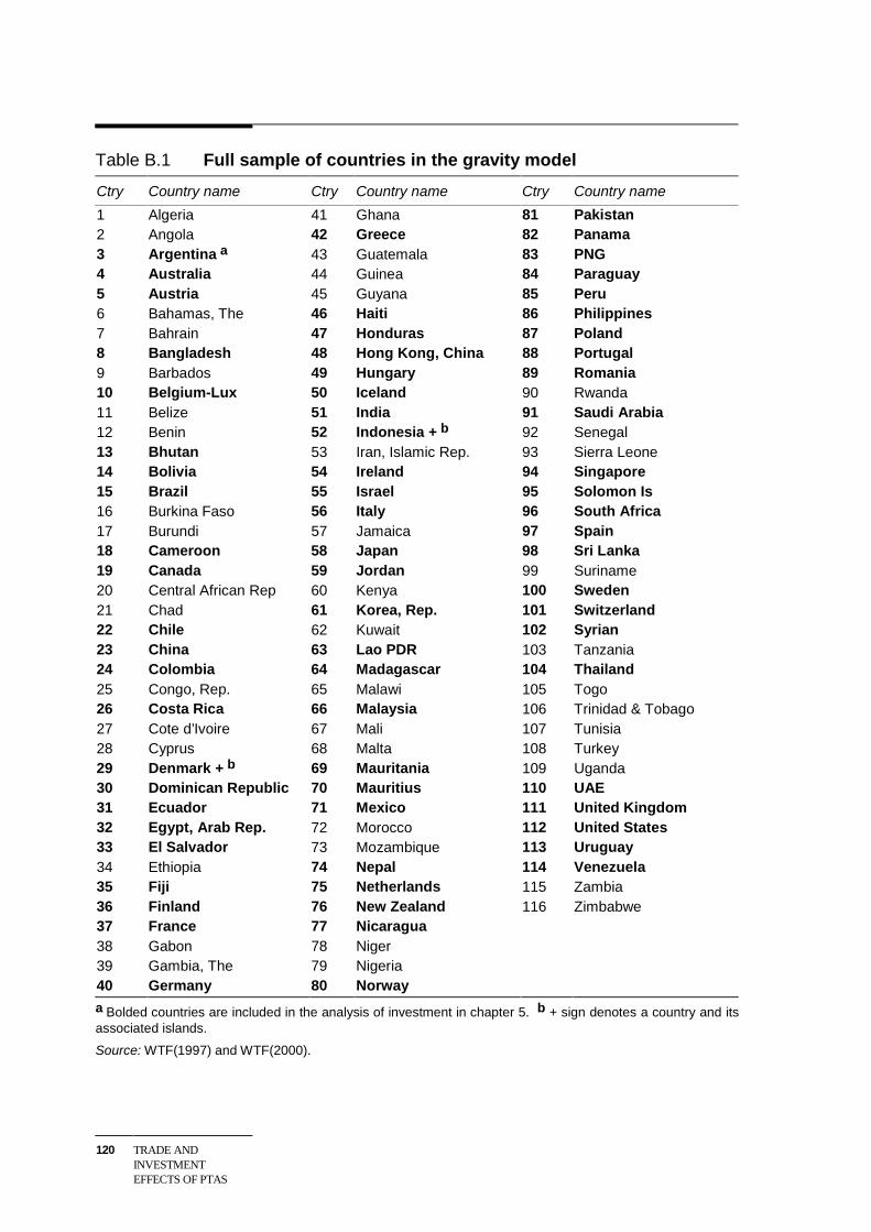
120 TRADE ANDINVESTMENTEFFECTS OF PTAS
Table B.1 Full sample of countries in the gravity model
Ctry Country name Ctry Country name Ctry Country name
1 Algeria 41 Ghana 81 Pakistan2 Angola 42 Greece 82 Panama3 Argentina a 43 Guatemala 83 PNG4 Australia 44 Guinea 84 Paraguay5 Austria 45 Guyana 85 Peru6 Bahamas, The 46 Haiti 86 Philippines7 Bahrain 47 Honduras 87 Poland8 Bangladesh 48 Hong Kong, China 88 Portugal9 Barbados 49 Hungary 89 Romania10 Belgium-Lux 50 Iceland 90 Rwanda11 Belize 51 India 91 Saudi Arabia12 Benin 52 Indonesia + b 92 Senegal13 Bhutan 53 Iran, Islamic Rep. 93 Sierra Leone14 Bolivia 54 Ireland 94 Singapore15 Brazil 55 Israel 95 Solomon Is16 Burkina Faso 56 Italy 96 South Africa17 Burundi 57 Jamaica 97 Spain18 Cameroon 58 Japan 98 Sri Lanka19 Canada 59 Jordan 99 Suriname20 Central African Rep 60 Kenya 100 Sweden21 Chad 61 Korea, Rep. 101 Switzerland22 Chile 62 Kuwait 102 Syrian23 China 63 Lao PDR 103 Tanzania24 Colombia 64 Madagascar 104 Thailand25 Congo, Rep. 65 Malawi 105 Togo26 Costa Rica 66 Malaysia 106 Trinidad & Tobago27 Cote d’Ivoire 67 Mali 107 Tunisia28 Cyprus 68 Malta 108 Turkey29 Denmark + b 69 Mauritania 109 Uganda30 Dominican Republic 70 Mauritius 110 UAE31 Ecuador 71 Mexico 111 United Kingdom32 Egypt, Arab Rep. 72 Morocco 112 United States33 El Salvador 73 Mozambique 113 Uruguay34 Ethiopia 74 Nepal 114 Venezuela35 Fiji 75 Netherlands 115 Zambia36 Finland 76 New Zealand 116 Zimbabwe37 France 77 Nicaragua38 Gabon 78 Niger39 Gambia, The 79 Nigeria40 Germany 80 Norway
a Bolded countries are included in the analysis of investment in chapter 5. b + sign denotes a country and itsassociated islands.
Source: WTF(1997) and WTF(2000).
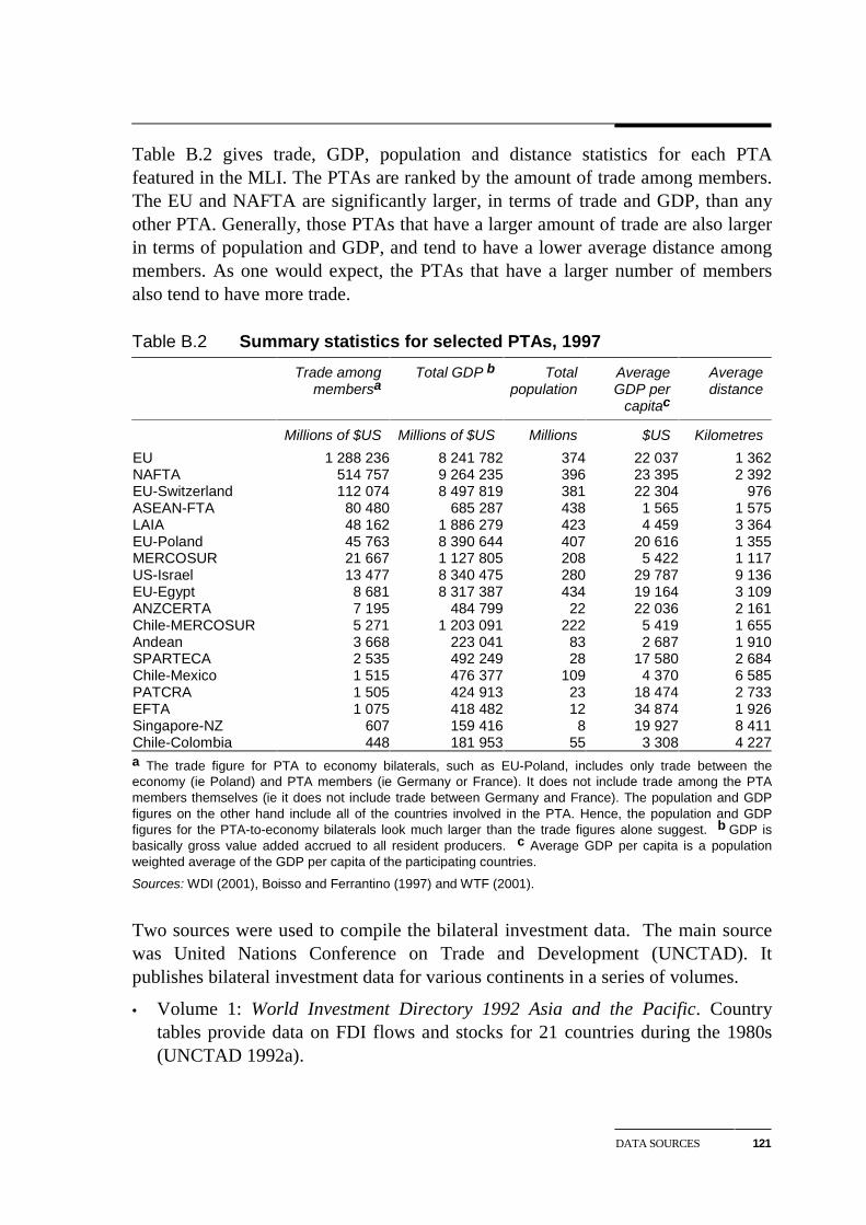
DATA SOURCES 121
Table B.2 gives trade, GDP, population and distance statistics for each PTAfeatured in the MLI. The PTAs are ranked by the amount of trade among members.The EU and NAFTA are significantly larger, in terms of trade and GDP, than anyother PTA. Generally, those PTAs that have a larger amount of trade are also largerin terms of population and GDP, and tend to have a lower average distance amongmembers. As one would expect, the PTAs that have a larger number of membersalso tend to have more trade.
Table B.2 Summary statistics for selected PTAs, 1997
Trade amongmembersa
Total GDP b Totalpopulation
AverageGDP per
capitac
Averagedistance
Millions of $US Millions of $US Millions $US Kilometres
EU 1 288 236 8 241 782 374 22 037 1 362NAFTA 514 757 9 264 235 396 23 395 2 392EU-Switzerland 112 074 8 497 819 381 22 304 976ASEAN-FTA 80 480 685 287 438 1 565 1 575LAIA 48 162 1 886 279 423 4 459 3 364EU-Poland 45 763 8 390 644 407 20 616 1 355MERCOSUR 21 667 1 127 805 208 5 422 1 117US-Israel 13 477 8 340 475 280 29 787 9 136EU-Egypt 8 681 8 317 387 434 19 164 3 109ANZCERTA 7 195 484 799 22 22 036 2 161Chile-MERCOSUR 5 271 1 203 091 222 5 419 1 655Andean 3 668 223 041 83 2 687 1 910SPARTECA 2 535 492 249 28 17 580 2 684Chile-Mexico 1 515 476 377 109 4 370 6 585PATCRA 1 505 424 913 23 18 474 2 733EFTA 1 075 418 482 12 34 874 1 926Singapore-NZ 607 159 416 8 19 927 8 411Chile-Colombia 448 181 953 55 3 308 4 227a The trade figure for PTA to economy bilaterals, such as EU-Poland, includes only trade between theeconomy (ie Poland) and PTA members (ie Germany or France). It does not include trade among the PTAmembers themselves (ie it does not include trade between Germany and France). The population and GDPfigures on the other hand include all of the countries involved in the PTA. Hence, the population and GDPfigures for the PTA-to-economy bilaterals look much larger than the trade figures alone suggest. b GDP isbasically gross value added accrued to all resident producers. c Average GDP per capita is a populationweighted average of the GDP per capita of the participating countries.
Sources: WDI (2001), Boisso and Ferrantino (1997) and WTF (2001).
Two sources were used to compile the bilateral investment data. The main sourcewas United Nations Conference on Trade and Development (UNCTAD). Itpublishes bilateral investment data for various continents in a series of volumes.
• Volume 1: World Investment Directory 1992 Asia and the Pacific. Countrytables provide data on FDI flows and stocks for 21 countries during the 1980s(UNCTAD 1992a).
122 TRADE ANDINVESTMENTEFFECTS OF PTAS
• Volume 2: World Investment Directory 1992 Central and Eastern Europe.Country tables provide data on FDI flows and stocks for 26 countries during the1980s (UNCTAD 1992b).
• Volume 3: World Investment Directory 1993 Developed economies. Countrytables provide data on FDI flows and stocks for 22 countries during the 1980s(UNCTAD 1993).
• Volume 4: World Investment Directory 1994 Latin America and the Caribbean.Country tables provide data on FDI flows and stocks for 24 countries during the1980s (UNCTAD 1994).
• Volume 5: World Investment Directory 1996 Africa. Country tables providedata on FDI flows and stocks for 53 countries during the late 1980s and early1990s (UNCTAD 1997a).
• Volume 6: World Investment Directory 1996 West Asia. Country tables providedata on FDI flows and stocks for 15 countries during the late 1980s and early1990s (UNCTAD 1997b).
• Volume 7: World Investment Directory 2000 Asia and the Pacific. Countrytables provide data on FDI flows and stocks for 23 countries during the 1990s(UNCTAD 2000).
The primary source of the bilateral FDI data for UNCTAD was respective countryfinance departments, central banks, and TNC operations.
OECD collects FDI data for 23 countries. For many developed countries, the OECDdata were used to extend the UNCTAD bilateral data which ended at 1991. TheOECD data are available electronically. The UNCTAD investment data are notavailable electronically. UNCTAD use a country-specific definition of FDI and theOECD uses a semi-standardised definition of FDI — the OECD benchmarkdefinition.1
The bilateral FDI data have a number of limitations (Bellak 1998).
• There is little consistency in the attribution of nationality to transit investment, ieFDI undertaken by a regional headquarters rather than a parent company.
• The coverage is limited, even in developed countries.2
1 Not all OECD countries comply with the OECD benchmark definition, which requires 10 per
cent or more of the ordinary shares or voting power for investment to be ‘direct’. The OECDuses the ‘fully consolidated’ system, ie the subsidiary of an subsidiary is automatically asubsidiary.
2 The UK statistics exclude oil and the financial sector in most years. Given the importance of theUnited Kingdom as a financial centre of the world and as an oil trading country, this leads to aserious underestimation of the United Kingdom’s foreign investment.
DATA SOURCES 123
• The data are sporadic for developing and under developed countries.
• Stock data are imputed from flows data by simple cumulative addition, with noallowance for depreciation.
B.2 Explanatory variables
Most of the other data on the explanatory variables were sourced from WorldBank’s World Development Indicators 2001 database (WDI 2001). The WDIdatabase covers a wide range of time series data on social and economic indicators,including data on population, arable land and exchange rates. The remaining datawere sourced from similar gravity model studies. The details are as follows.
The GDP data measure gross domestic product at purchasing power parity (PPP).Most of the GDP data were sourced from the World Bank’s World DevelopmentIndicators (WDI 2001). GDP is basically gross value added accrued to all residentproducers, measured in local currency units. Insufficient data were available forsome economies and some years, and data were supplemented from the IMF and theOECD (IMF 2001 and OECD 2001).
The GDP data were converted to current international dollars using PPP conversionfactors from the WDI. There were no data from 1970 to 1974 and the data wereinsufficient for some economies from 1975 to 1997. The PPP conversion factorswere estimated, for the missing economies and years, by extrapolating the data backto 1970. GDP at PPP was then calculated by dividing GDP in local currency unitsby the PPP conversion factors. GDP per capita was calculated by dividing GDP bypopulation for each economy.
Population data were sourced from the WDI 2001. Population is measured as themid-year population and counts all residents of an economy regardless of legalstatus or citizenship.
The primary source of the distance data was Boisso and Ferrantino (1997), whocalculate the distance between the two largest cities. Distance is measured inkilometres and is the great circle distance or ‘as the crow flies’. Data were notavailable for a number of smaller economies, and data for the missing economieswere taken from Haveman (2000), who measures the distance between capitalcities.
The measure of linguistic similarity was sourced from Boisso and Ferantino (1997).The variable measures the degree of commonality in the languages that are spokenbetween any two economies. The measure takes a value ranging from 0 to 10 000,depending on the percentage of people in each economy who speak the same
124 TRADE ANDINVESTMENTEFFECTS OF PTAS
language. In general, the percentage of people speaking the same language in oneeconomy is multiplied by the percentage of people speaking that language in theother economy. The linguistic similarity index receives a value of zero when thetwo economies are completely dissimilar and a value of 10 000 when the entirepopulations of the two economies speak the same language.
The data for colonial and currency links were sourced from Frankel and Rose(2000). Two dummy variables were formed, the first with a value of one where oneeconomy colonised the other economy and zero otherwise, the second with a valueone when the two countries share a currency, and zero otherwise.
Most of the adjacency data were obtained from Boisso and Ferrantino (1997). Datafrom Haveman (2000) were used to supplement the Boisso and Ferrantino data inorder to fill some gaps in the economy coverage. The adjacency variable is adummy with a value one when the two economies share a border, and zerootherwise.
The data for the island and landlocked variables were taken from Times (1993).Two dummy variables were formed, one with a value one where an economy is anisland and zero otherwise, the other with a value of one when the economy islandlocked and zero otherwise.
Exchange rate data were sourced from WDI (2001). The exchange rate is measuredas the period average exchange rate — the number of local currency units that canbe traded for one US dollar. A bilateral exchange rate (the value of a unit of theexporter’s currency in terms of the importer’s currency) was calculated by dividingthe importer’s $US exchange rate by the exporter’s $US exchange rate.
The tariff data were sourced from the TRAINS database (UNCTAD 2001). Thevariable is measured as the simple average tariff rate — total value divided by thenumber of tariff lines.
The Member Liberalisation Index (MLI) measures the extent of liberalisation withina PTA. The value of the MLI for a bilateral trade flow depends on wether the twoeconomies are members of the same PTA. A variable was formed that allocates thescore from the MLI where the two economies are members of the same PTA and inall other cases allocates a score of zero. When the two economies have more thanone PTA in common, an a priori judgement was made as to which PTA was morelikely to dictate the trading conditions between the two countries. Appendix Aprovides detailed information on how the index was calculated.
ECONOMETRICESTIMATION ANDISSUES
125
C Econometric estimation and issues
In the gravity model of bilateral trade, the sample is limited by censoring. Bilateralexports cannot take a negative value. To account for the truncated distribution ofpossible values for the dependent variable, a censored regression technique is usedin this study.
While techniques for estimating single equation censored regression models havebeen available in a number of popular statistics and econometric software packagesfor quite some time, estimation in a panel context is a recent phenomena. Theappendix first discusses fixed versus random effects specifications, and thendiscusses estimation of a Tobit model with fixed effects. Finally it discusses therelationship between the resulting parameter estimates and marginal effects.
C.1 Fixed versus random effects specifications
The fixed and random effects models are alternative ways of accounting forunobserved heterogeneity. The random effects model requires an impracticalorthogonality assumption — it requires that the unobserved effects be uncorrelatedwith the included explanatory variables. The fixed effects model relaxes thisorthogonality assumption, but is widely recognised to suffer from an incidentalparameter problem in a panel context — the estimator is inconsistent because theasymptotic variance of the estimator of the main parameters is a function of the sizeof the fixed groups (Lancaster 2000). How serious this problem is in practical termsremains to be established in the literature, although it appears to be worse in a non-linear (eg Tobit) context.
Statistical tests are available to choose between fixed and random effectsspecifications. Hausman’s statistic for testing random versus fixed effects is appliedfor the positive trade values in this study (Baltagi 1995 and Greene 2000). TheHausman statistic tests for the orthogonality of the random effects and theregressors, and is thus a test for misspecification. A significant test statistic reveals ahigh importance of individual specific effects and their correlation with theregressors. In such a case, the random effect estimates are significantly inconsistent.In a specification that allowed both the fixed and random effects to vary byexporting and importing country pair, the estimated Hausman test statistic was

126 TRADE ANDINVESTMENTEFFECTS OF PTAS
3342.7, which was more than the critical value at the 5 per cent level (34.5). Thusthe random effects specification was rejected.1 This study has therefore adopted afixed effects specification within a Tobit model.
C.2 Tobit model with fixed effects
Only few studies have discussed and estimated fixed effects Tobit models —Honere and Kyriazidou (2000) and Greene (2002).
Honere (1992) initially proposed artificially censoring the dependent variable insuch a way that the fixed effects could be differenced out. In a later study, Honereand Kyriazidou (2000) used semiparametric and generalised methods of momentsapproaches with latent heterogeneity. The practical limitation of their estimator isthat although it provides estimates of the primary slope parameters, it does notprovide estimates for the full set of model parameters and thus precludescomputation of marginal effects (elasticities), probabilities of predictions for thedependent variable and their standard errors.
Greene (2002) argued that in spite of several shortcomings, the conventional(unconditional) fixed effects estimator has some merits in a Tobit panel context. Heobtained results that show the slope estimates in the Tobit model do not appear to beaffected by the incidental parameters problem. However, the variance of the modelestimate is affected, and this is a crucial parameter in a Tobit model for inferenceand analysis purposes. But the bias in the variance appears to fall fairly quickly asthe number of time periods in the panel increases. This study has twenty-eight yearsof data in the panel and thus overcomes the small time period bias.
The fixed effects estimator is nevertheless inconsistent because its variance does notconverge to zero as the sample size increases. Greene (2002) showed that as aresult, there is clearly some downward bias in all the estimated standard errors ofthe Tobit model parameters. The implication of this is that test statistics such as theWald statistic will tend to be too large.
In addition, there may be a small sample bias in the Tobit fixed effectsspecification. Greene (2002) showed that increasing the sample size from 100 to1000 did little to remove this small sample bias, but increasing the group size from2 to 20 had a very large effect. He concluded that the bias was primarily a problemin panels with a small number of time periods. Again, the reasonably large number
1 Maddala (1987) and Baltagi (1995) argued that the fixed effects estimator derived from the linear
panel model may not carry to non-linear models.
ECONOMETRICESTIMATION ANDISSUES
127
of time periods in the current study suggest that small sample bias may not be aproblem.
C.3 Marginal effects
The Tobit model can be viewed as consisting of two parts. The first specifies astructural relationship between the explanatory variables and a hypothetical or a‘latent’ underlying dependent variable, the distribution of which is not censored.The second part specifies how the observations on this latent dependent variable arecensored. The interpretation of Tobit estimates depends on whether one is interestedin latent or censored outcomes. If one is interested in latent outcomes (unobservednon-positive trade flows), the Tobit estimates obtained can be directly interpreted asthe marginal effects of the explanatory variables on the dependent variable. If theinterest lies in the determinants of observed trade flows, as it does here, themarginal effects of the explanatory variables on censored outcomes need to beestimated separately. Table C.1 provides the estimated marginal effectscorresponding to the raw maximum likelihood Tobit estimates of table D.2 inappendix D.
The results confirm that the marginal effects differ from the raw Tobit estimates.However, for any particular PTA, the marginal effects of the three PTA dummiestend to be roughly proportional to the corresponding raw parameter estimates.Therefore, in practice, conclusions about whether the net trade effects of a particularPTA are positive or negative are invariant to whether the marginal effects or the rawparameter estimates are used.
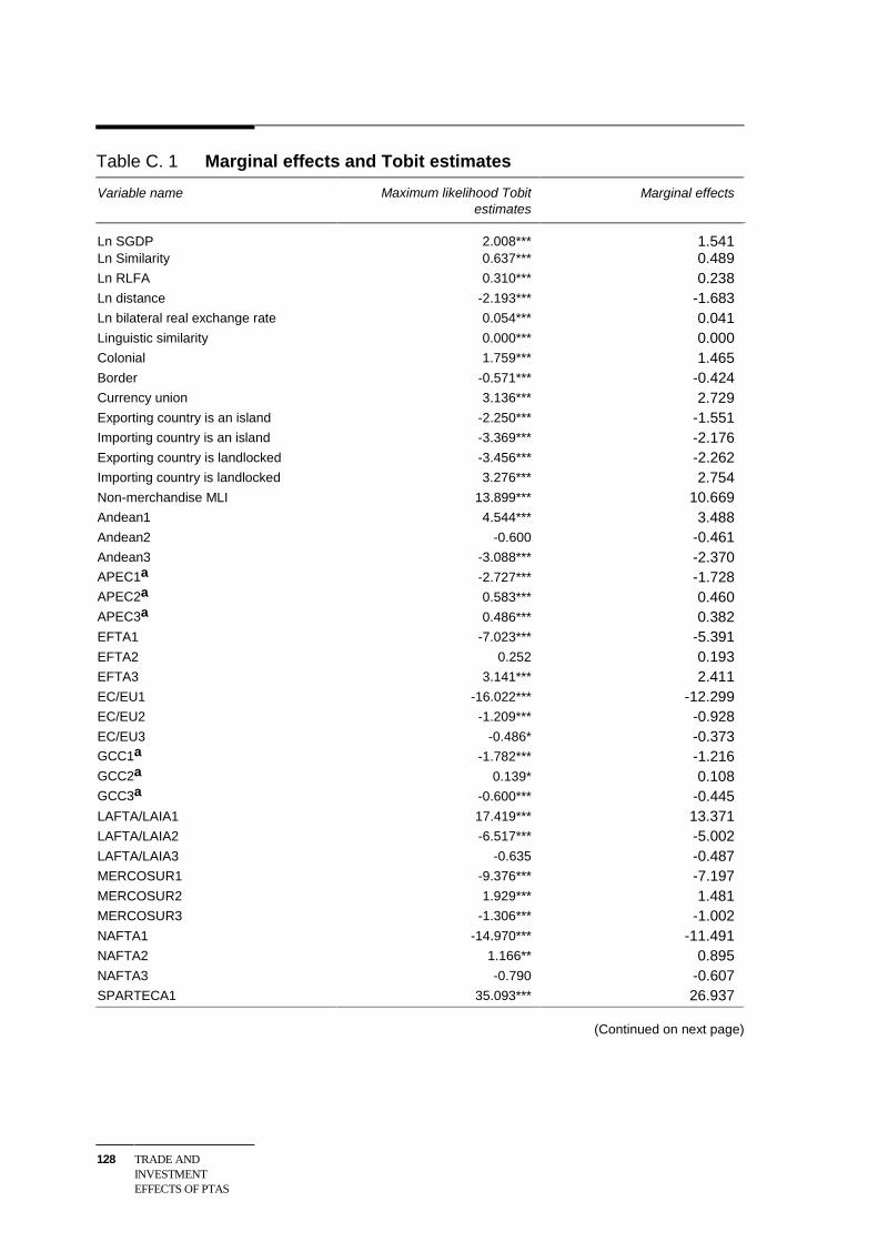
128 TRADE ANDINVESTMENTEFFECTS OF PTAS
Table C. 1 Marginal effects and Tobit estimates
Variable name Maximum likelihood Tobitestimates
Marginal effects
Ln SGDP 2.008*** 1.541Ln Similarity 0.637*** 0.489Ln RLFA 0.310*** 0.238Ln distance -2.193*** -1.683Ln bilateral real exchange rate 0.054*** 0.041Linguistic similarity 0.000*** 0.000Colonial 1.759*** 1.465Border -0.571*** -0.424Currency union 3.136*** 2.729Exporting country is an island -2.250*** -1.551Importing country is an island -3.369*** -2.176Exporting country is landlocked -3.456*** -2.262Importing country is landlocked 3.276*** 2.754Non-merchandise MLI 13.899*** 10.669Andean1 4.544*** 3.488Andean2 -0.600 -0.461Andean3 -3.088*** -2.370APEC1a -2.727*** -1.728APEC2a 0.583*** 0.460APEC3a 0.486*** 0.382EFTA1 -7.023*** -5.391EFTA2 0.252 0.193EFTA3 3.141*** 2.411EC/EU1 -16.022*** -12.299EC/EU2 -1.209*** -0.928EC/EU3 -0.486* -0.373GCC1a -1.782*** -1.216GCC2a 0.139* 0.108GCC3a -0.600*** -0.445LAFTA/LAIA1 17.419*** 13.371LAFTA/LAIA2 -6.517*** -5.002LAFTA/LAIA3 -0.635 -0.487MERCOSUR1 -9.376*** -7.197MERCOSUR2 1.929*** 1.481MERCOSUR3 -1.306*** -1.002NAFTA1 -14.970*** -11.491NAFTA2 1.166** 0.895NAFTA3 -0.790 -0.607SPARTECA1 35.093*** 26.937
(Continued on next page)
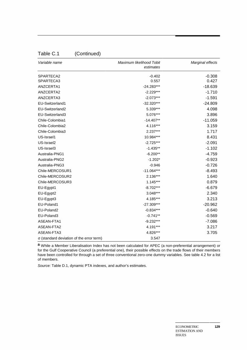
ECONOMETRICESTIMATION ANDISSUES
129
Table C.1 (Continued)
Variable name Maximum likelihood Tobitestimates
Marginal effects
SPARTECA2 -0.402 -0.308SPARTECA3 0.557 0.427ANZCERTA1 -24.283*** -18.639ANZCERTA2 -2.229*** -1.710ANZCERTA3 -2.073*** -1.591EU-Switzerland1 -32.320*** -24.809EU-Switzerland2 5.339*** 4.098EU-Switzerland3 5.076*** 3.896Chile-Colombia1 -14.407** -11.059Chile-Colombia2 4.116*** 3.159Chile-Colombia3 2.237*** 1.717US-Israel1 10.984*** 8.431US-Israel2 -2.725*** -2.091US-Israel3 -1.435** -1.102Australia-PNG1 -6.200** -4.759Australia-PNG2 -1.202* -0.923Australia-PNG3 -0.946 -0.726Chile-MERCOSUR1 -11.064*** -8.493Chile-MERCOSUR2 2.136*** 1.640Chile-MERCOSUR3 1.145*** 0.879EU-Egypt1 -8.702*** -6.679EU-Egypt2 3.048*** 2.340EU-Egypt3 4.185*** 3.213EU-Poland1 -27.309*** -20.962EU-Poland2 -0.834*** -0.640EU-Poland3 -0.741** -0.569ASEAN-FTA1 -9.232*** -7.086ASEAN-FTA2 4.191*** 3.217ASEAN-FTA3 4.826*** 3.705σ (standard deviation of the error term) 3.547
a While a Member Liberalisation Index has not been calculated for APEC (a non-preferential arrangement) orfor the Gulf Cooperative Council (a preferential one), their possible effects on the trade flows of their membershave been controlled for through a set of three conventional zero-one dummy variables. See table 4.2 for a listof members.
Source: Table D.1, dynamic PTA indexes, and author’s estimates.

130 TRADE ANDINVESTMENTEFFECTS OF PTAS
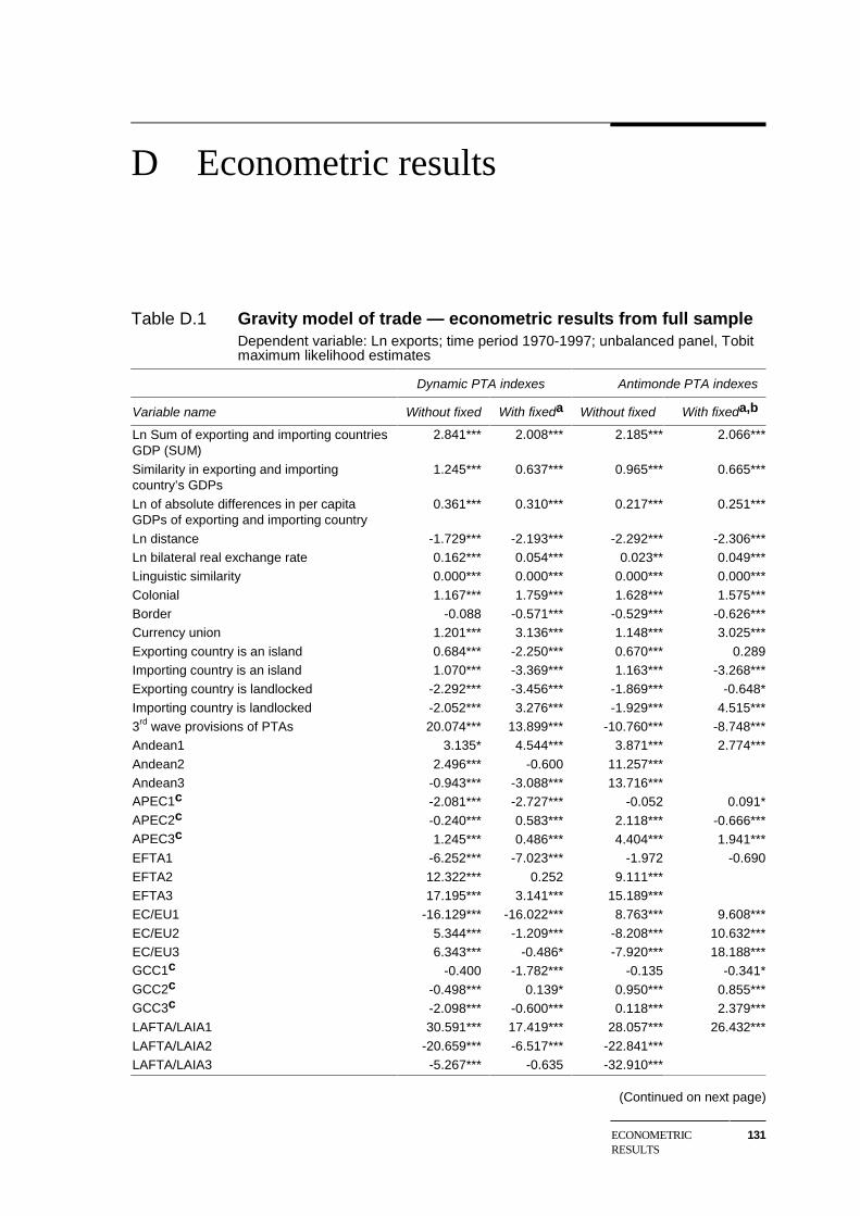
ECONOMETRICRESULTS
131
D Econometric results
Table D.1 Gravity model of trade — econometric results from full sampleDependent variable: Ln exports; time period 1970-1997; unbalanced panel, Tobitmaximum likelihood estimates
Dynamic PTA indexes Antimonde PTA indexes
Variable name Without fixed With fixeda Without fixed With fixeda,b
Ln Sum of exporting and importing countriesGDP (SUM)
2.841*** 2.008*** 2.185*** 2.066***
Similarity in exporting and importingcountry’s GDPs
1.245*** 0.637*** 0.965*** 0.665***
Ln of absolute differences in per capitaGDPs of exporting and importing country
0.361*** 0.310*** 0.217*** 0.251***
Ln distance -1.729*** -2.193*** -2.292*** -2.306***Ln bilateral real exchange rate 0.162*** 0.054*** 0.023** 0.049***Linguistic similarity 0.000*** 0.000*** 0.000*** 0.000***
Colonial 1.167*** 1.759*** 1.628*** 1.575***Border -0.088 -0.571*** -0.529*** -0.626***Currency union 1.201*** 3.136*** 1.148*** 3.025***
Exporting country is an island 0.684*** -2.250*** 0.670*** 0.289Importing country is an island 1.070*** -3.369*** 1.163*** -3.268***Exporting country is landlocked -2.292*** -3.456*** -1.869*** -0.648*
Importing country is landlocked -2.052*** 3.276*** -1.929*** 4.515***3rd wave provisions of PTAs 20.074*** 13.899*** -10.760*** -8.748***Andean1 3.135* 4.544*** 3.871*** 2.774***
Andean2 2.496*** -0.600 11.257***Andean3 -0.943*** -3.088*** 13.716***APEC1c -2.081*** -2.727*** -0.052 0.091*APEC2c -0.240*** 0.583*** 2.118*** -0.666***APEC3c 1.245*** 0.486*** 4.404*** 1.941***EFTA1 -6.252*** -7.023*** -1.972 -0.690
EFTA2 12.322*** 0.252 9.111***EFTA3 17.195*** 3.141*** 15.189***EC/EU1 -16.129*** -16.022*** 8.763*** 9.608***
EC/EU2 5.344*** -1.209*** -8.208*** 10.632***EC/EU3 6.343*** -0.486* -7.920*** 18.188***GCC1c -0.400 -1.782*** -0.135 -0.341*GCC2c -0.498*** 0.139* 0.950*** 0.855***GCC3c -2.098*** -0.600*** 0.118*** 2.379***LAFTA/LAIA1 30.591*** 17.419*** 28.057*** 26.432***
LAFTA/LAIA2 -20.659*** -6.517*** -22.841***LAFTA/LAIA3 -5.267*** -0.635 -32.910***
(Continued on next page)
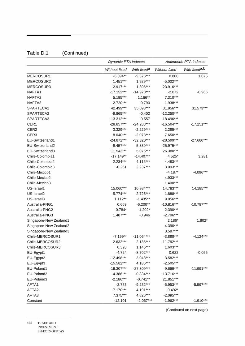
132 TRADE ANDINVESTMENTEFFECTS OF PTAS
Table D.1 (Continued)
Dynamic PTA indexes Antimonde PTA indexes
Without fixed With fixeda Without fixed With fixeda,b
MERCOSUR1 -6.894** -9.376*** 0.800 1.075MERCOSUR2 1.451*** 1.929*** -5.002***
MERCOSUR3 2.917*** -1.306*** 23.916***NAFTA1 -17.152*** -14.970*** -2.072 -0.966NAFTA2 5.195*** 1.166** 7.310***
NAFTA3 -2.720*** -0.790 -1.938***SPARTECA1 42.499*** 35.093*** 31.956*** 31.573***SPARTECA2 -9.865*** -0.402 -12.250***
SPARTECA3 -13.312*** 0.557 -18.496***CER1 -28.857*** -24.283*** -16.504*** -17.251***CER2 3.329*** -2.229*** 2.285***
CER3 8.040*** -2.073*** 7.650***EU-Switzerland1 -24.872*** -32.320*** -28.599*** -27.680***EU-Switzerland2 9.457*** 5.339*** 25.975***
EU-Switzerland3 11.542*** 5.076*** 26.380***Chile-Colombia1 -17.149** -14.407** 4.525* 3.281Chile-Colombia2 2.234*** 4.116*** -4.483***
Chile-Colombia3 -0.251 2.237*** 3.093***Chile-Mexico1 -4.187* -4.096***Chile-Mexico2 -4.933***
Chile-Mexico3 1.400***US-Israel1 15.060*** 10.984*** 14.783*** 14.185***US-Israel2 -5.774*** -2.725*** 1.888***
US-Israel3 1.112** -1.435** 9.056***Australia-PNG1 0.669 -6.200** -10.816*** -10.797***Australia-PNG2 0.784* -1.202* 2.390***
Australia-PNG3 1.487*** -0.946 -2.706***Singapore-New Zealand1 2.186* 1.802*Singapore-New Zealand2 4.390***
Singapore-New Zealand3 3.587***Chile-MERCOSUR1 -7.199** -11.064*** -3.888*** -4.124***Chile-MERCOSUR2 2.632*** 2.136*** 11.792***
Chile-MERCOSUR3 0.328 1.145*** 1.603***EU-Egypt1 -4.724 -8.702*** 0.622 -0.055EU-Egypt2 -12.498*** 3.048*** 3.582***
EU-Egypt3 -15.582*** 4.185*** -2.505***EU-Poland1 -19.307*** -27.309*** -9.699*** -11.991***EU-Poland2 -4.386*** -0.834*** 13.716***
EU-Poland3 -2.186*** -0.741** 21.851***AFTA1 -3.783 -9.232*** -5.953*** -5.597***AFTA2 7.170*** 4.191*** 0.492*
AFTA3 7.375*** 4.826*** -2.095***Constant -12.101 -2.067*** -1.962*** -1.910***
(Continued on next page)
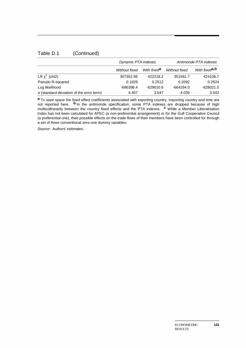
ECONOMETRICRESULTS
133
Table D.1 (Continued)
Dynamic PTA indexes Antimonde PTA indexes
Without fixed With fixeda Without fixed With fixeda,b
LR χ2 (chi2) 307352.95 422218.2 351561.7 424106.7
Pseudo R-squared 0.1829 0.2512 0.2092 0.2524Log likelihood -686398.4 -629010.8 -664294.0 -628021.5
σ (standard deviation of the error term) 4.407 3.547 4.036 3.542
a To save space the fixed effect coefficients associated with exporting country, importing country and time arenot reported here. b In the antimonde specification, some PTA indexes are dropped because of highmulticollinearity between the country fixed effects and the PTA indexes. c While a Member LiberalisationIndex has not been calculated for APEC (a non-preferential arrangement) or for the Gulf Cooperative Council(a preferential one), their possible effects on the trade flows of their members have been controlled for througha set of three conventional zero-one dummy variables.
Source: Authors’ estimates.
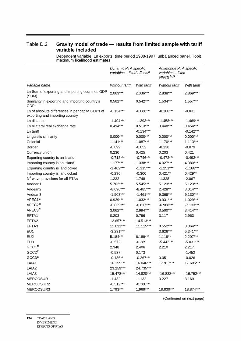
134 TRADE ANDINVESTMENTEFFECTS OF PTAS
Table D.2 Gravity model of trade — results from limited sample with tariffvariable includedDependent variable: Ln exports; time period 1988-1997; unbalanced panel, Tobitmaximum likelihood estimates
Dynamic PTA specificvariables – fixed effectsa
Antimonde PTA specificvariables – fixedeffectsa,b
Variable name Without tariff With tariff Without tariff With tariff
Ln Sum of exporting and importing countries GDP(SUM)
2.063*** 2.036*** 2.838*** 2.869***
Similarity in exporting and importing country’sGDPs
0.562*** 0.542*** 1.534*** 1.557***
Ln of absolute differences in per capita GDPs ofexporting and importing country
-0.154*** -0.086*** -0.100*** -0.031
Ln distance -1.404*** -1.393*** -1.458*** -1.469***Ln bilateral real exchange rate 0.494*** 0.513*** 0.448*** 0.454***
Ln tariff -0.134*** -0.142***Linguistic similarity 0.000*** 0.000*** 0.000*** 0.000***Colonial 1.141*** 1.087*** 1.170*** 1.113***
Border -0.099 -0.052 -0.138 -0.079Currency union 0.230 0.425 0.203 0.421Exporting country is an island -0.718*** -0.746*** -0.472*** -0.492***
Importing country is an island 1.177*** 1.338*** 4.027*** 4.380***Exporting country is landlocked -1.402*** -1.315*** -1.251*** -1.166***Importing country is landlocked -0.236 -0.300 0.421** 0.429**
3rd wave provisions for all PTAs 1.222 1.748 -1.328 -2.067Andean1 5.702*** 5.545*** 5.123*** 5.123***Andean2 -8.696*** -8.485*** 2.428** 3.014***
Andean3 -1.503*** -1.461*** 9.368*** 9.130***APEC1c 0.929*** 1.032*** 0.931*** 1.029***APEC2c -0.839*** -0.817*** -6.988*** -7.133***APEC3c 3.062*** 2.994*** 3.500*** 3.414***EFTA1 0.203 0.796 3.117 2.963EFTA2 12.657*** 14.513***
EFTA3 11.631*** 11.115*** 8.552*** 8.364***EU1 -3.231*** 3.626*** 5.341***EU2 5.184*** 6.189*** 1.118** 2.207***
EU3 -0.572 -0.289 -5.442*** -5.031***GCC1c 2.348 2.406 2.210 2.217GCC2c -0.537 0.173 -1.452GCC3c -0.186** -0.267*** 0.051 -0.026LAIA1 16.159*** 16.046*** 17.917*** 17.605***LAIA2 23.259*** 24.735***
LAIA3 15.478*** 14.820*** -16.838*** -16.752***MERCOSUR1 -1.432 -1.132 3.227 3.169MERCOSUR2 -8.512*** -8.380***
MERCOSUR3 1.793*** 1.969*** 18.830*** 18.874***
(Continued on next page)
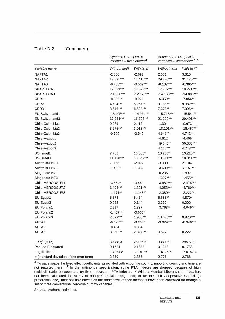
ECONOMETRICRESULTS
135
Table D.2 (Continued)
Dynamic PTA specificvariables – fixed effectsa
Antimonde PTA specificvariables – fixed effectsa,b
Variable name Without tariff With tariff Without tariff With tariff
NAFTA1 -2.800 -2.692 2.551 3.315NAFTA2 13.591*** 14.416*** 29.870*** 31.170***NAFTA3 -8.453*** -8.562*** -8.137*** -8.385***
SPARTECA1 17.033*** 18.523*** 17.702*** 19.271***SPARTECA3 -11.930*** -12.128*** -14.163*** -14.880***CER1 -8.356** -8.976 -6.959** -7.056**
CER2 4.704*** 5.267** 9.138*** 9.382***CER3 8.616*** 8.523*** 7.378*** 7.396***EU-Switzerland1 -15.405*** -14.934*** -15.718*** -15.541***
EU-Switzerland3 17.254*** 16.723*** 21.229*** 20.401***Chile-Colombia1 0.079 0.416 -1.304 -0.673Chile-Colombia2 3.275*** 3.013*** -18.101*** -18.457***
Chile-Colombia3 -0.705 -0.545 4.641*** 4.742***Chile-Mexico1 -4.612 -4.405Chile-Mexico2 49.545*** 50.383***
Chile-Mexico3 4.116*** 4.243***US-Israel1 7.763 10.386* 10.255* 13.218**US-Israel3 11.120*** 10.649*** 10.811*** 10.341***
Australia-PNG1 -1.166 -2.097 -3.080 -5.104Australia-PNG3 -1.492* -1.382 -3.609*** -3.157***Singapore-NZ1 -0.235 1.892
Singapore-NZ3 1.307*** 1.455***Chile-MERCOSUR1 -3.654* -3.440 -3.682*** -3.478***Chile-MERCOSUR2 1.403*** 1.321*** -4.953*** -4.780***
Chile-MERCOSUR3 -1.171** -1.148** -2.080** -2.222**EU-Egypt1 5.573 5.454 5.688** 4.870*EU-Egypt3 0.682 0.144 0.336 0.006
EU-Poland1 2.517 1.837 -3.763** -4.049**EU-Poland2 -1.457*** -0.600*EU-Poland3 2.099*** 1.956*** 10.075*** 9.820***
AFTA1 -9.693*** -8.204* -9.629*** -8.946***AFTA2 -0.484 0.354AFTA3 3.060*** 2.827*** 0.572 0.222
LR χ2 (chi2) 32088.3 28186.5 33800.9 29892.8
Pseudo R-squared 0.1724 0.1656 0.1816 0.1756Log likelihood -77034.8 -71010.6 -76178.6 -7.0157.4
σ (standard deviation of the error term) 2.859 2.855 2.776 2.766
a To save space the fixed effect coefficients associated with exporting country, importing country and time arenot reported here. b In the antimonde specification, some PTA indexes are dropped because of highmulticollinearity between country fixed effects and PTA indexes. c While a Member Liberalisation Index hasnot been calculated for APEC (a non-preferential arrangement) or for the Gulf Cooperative Council (apreferential one), their possible effects on the trade flows of their members have been controlled for through aset of three conventional zero-one dummy variables.
Source: Authors’ estimates.
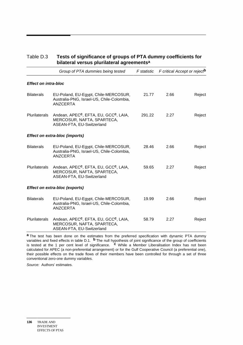
136 TRADE ANDINVESTMENTEFFECTS OF PTAS
Table D.3 Tests of significance of groups of PTA dummy coefficients forbilateral versus plurilateral agreementsa
Group of PTA dummies being tested F statistic F critical Accept or rejectb
Effect on intra-bloc
Bilaterals EU-Poland, EU-Egypt, Chile-MERCOSUR,Australia-PNG, Israel-US, Chile-Colombia,ANZCERTA
21.77 2.66 Reject
Plurilaterals Andean, APECc, EFTA, EU, GCCc, LAIA,MERCOSUR, NAFTA, SPARTECA,ASEAN-FTA, EU-Switzerland
291.22 2.27 Reject
Effect on extra-bloc (imports)
Bilaterals EU-Poland, EU-Egypt, Chile-MERCOSUR,Australia-PNG, Israel-US, Chile-Colombia,ANZCERTA
28.46 2.66 Reject
Plurilaterals Andean, APECc, EFTA, EU, GCCc, LAIA,MERCOSUR, NAFTA, SPARTECA,ASEAN-FTA, EU-Switzerland
59.65 2.27 Reject
Effect on extra-bloc (exports)
Bilaterals EU-Poland, EU-Egypt, Chile-MERCOSUR,Australia-PNG, Israel-US, Chile-Colombia,ANZCERTA
19.99 2.66 Reject
Plurilaterals Andean, APECc, EFTA, EU, GCCc, LAIA,MERCOSUR, NAFTA, SPARTECA,ASEAN-FTA, EU-Switzerland
58.79 2.27 Reject
a The test has been done on the estimates from the preferred specification with dynamic PTA dummyvariables and fixed effects in table D.1. b The null hypothesis of joint significance of the group of coefficientsis tested at the 1 per cent level of significance. c While a Member Liberalisation Index has not beencalculated for APEC (a non-preferential arrangement) or for the Gulf Cooperative Council (a preferential one),their possible effects on the trade flows of their members have been controlled for through a set of threeconventional zero-one dummy variables.
Source: Authors’ estimates.
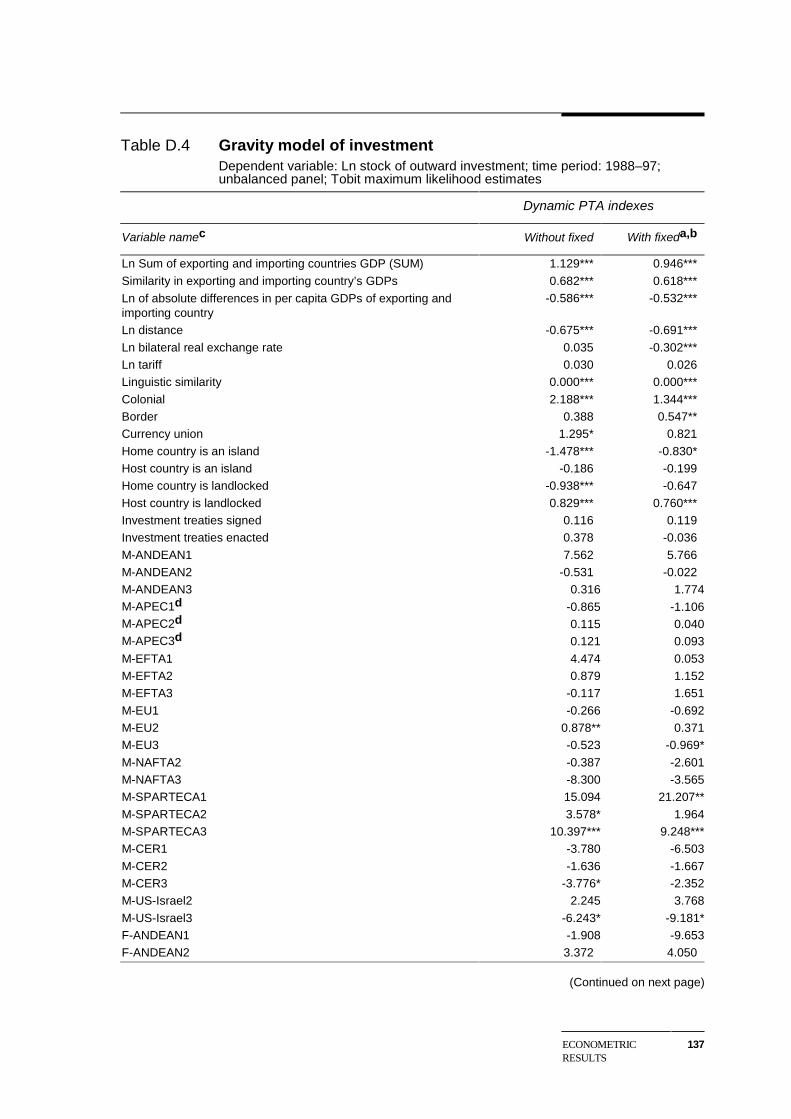
ECONOMETRICRESULTS
137
Table D.4 Gravity model of investmentDependent variable: Ln stock of outward investment; time period: 1988–97;unbalanced panel; Tobit maximum likelihood estimates
Dynamic PTA indexes
Variable namec Without fixed With fixeda,b
Ln Sum of exporting and importing countries GDP (SUM) 1.129*** 0.946***
Similarity in exporting and importing country’s GDPs 0.682*** 0.618***
Ln of absolute differences in per capita GDPs of exporting andimporting country
-0.586*** -0.532***
Ln distance -0.675*** -0.691***
Ln bilateral real exchange rate 0.035 -0.302***Ln tariff 0.030 0.026Linguistic similarity 0.000*** 0.000***
Colonial 2.188*** 1.344***Border 0.388 0.547**Currency union 1.295* 0.821
Home country is an island -1.478*** -0.830*Host country is an island -0.186 -0.199Home country is landlocked -0.938*** -0.647
Host country is landlocked 0.829*** 0.760***Investment treaties signed 0.116 0.119Investment treaties enacted 0.378 -0.036
M-ANDEAN1 7.562 5.766M-ANDEAN2 -0.531 -0.022M-ANDEAN3 0.316 1.774M-APEC1d -0.865 -1.106M-APEC2d 0.115 0.040M-APEC3d 0.121 0.093
M-EFTA1 4.474 0.053M-EFTA2 0.879 1.152M-EFTA3 -0.117 1.651
M-EU1 -0.266 -0.692M-EU2 0.878** 0.371M-EU3 -0.523 -0.969*
M-NAFTA2 -0.387 -2.601M-NAFTA3 -8.300 -3.565M-SPARTECA1 15.094 21.207**
M-SPARTECA2 3.578* 1.964M-SPARTECA3 10.397*** 9.248***M-CER1 -3.780 -6.503
M-CER2 -1.636 -1.667M-CER3 -3.776* -2.352M-US-Israel2 2.245 3.768
M-US-Israel3 -6.243* -9.181*F-ANDEAN1 -1.908 -9.653F-ANDEAN2 3.372 4.050
(Continued on next page)
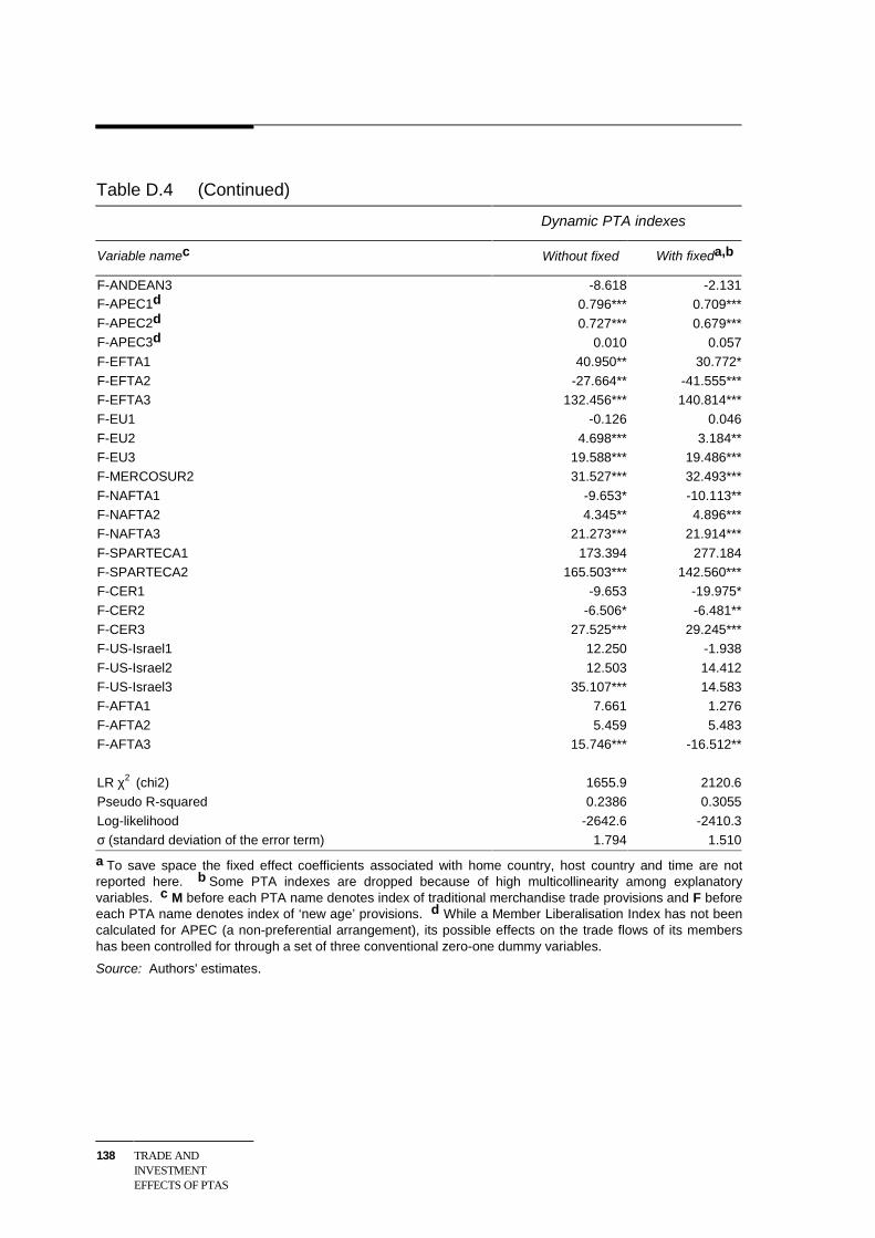
138 TRADE ANDINVESTMENTEFFECTS OF PTAS
Table D.4 (Continued)
Dynamic PTA indexes
Variable namec Without fixed With fixeda,b
F-ANDEAN3 -8.618 -2.131F-APEC1d 0.796*** 0.709***F-APEC2d 0.727*** 0.679***F-APEC3d 0.010 0.057F-EFTA1 40.950** 30.772*
F-EFTA2 -27.664** -41.555***F-EFTA3 132.456*** 140.814***F-EU1 -0.126 0.046
F-EU2 4.698*** 3.184**F-EU3 19.588*** 19.486***F-MERCOSUR2 31.527*** 32.493***
F-NAFTA1 -9.653* -10.113**F-NAFTA2 4.345** 4.896***F-NAFTA3 21.273*** 21.914***
F-SPARTECA1 173.394 277.184F-SPARTECA2 165.503*** 142.560***F-CER1 -9.653 -19.975*
F-CER2 -6.506* -6.481**F-CER3 27.525*** 29.245***F-US-Israel1 12.250 -1.938
F-US-Israel2 12.503 14.412F-US-Israel3 35.107*** 14.583F-AFTA1 7.661 1.276
F-AFTA2 5.459 5.483F-AFTA3 15.746*** -16.512**
LR χ2 (chi2) 1655.9 2120.6Pseudo R-squared 0.2386 0.3055
Log-likelihood -2642.6 -2410.3σ (standard deviation of the error term) 1.794 1.510
a To save space the fixed effect coefficients associated with home country, host country and time are notreported here. b Some PTA indexes are dropped because of high multicollinearity among explanatoryvariables. c M before each PTA name denotes index of traditional merchandise trade provisions and F beforeeach PTA name denotes index of ‘new age’ provisions. d While a Member Liberalisation Index has not beencalculated for APEC (a non-preferential arrangement), its possible effects on the trade flows of its membershas been controlled for through a set of three conventional zero-one dummy variables.
Source: Authors' estimates.
REFERENCES 139
References
ABS (Australian Bureau of Statistics) 2002, Balance of Payments, Australia:Regional Series 2000-01, Cat. No. 5338.0.
Aitken, N. 1973, ‘The effect of the EEC and EFTA on European trade: A temporalcross section analysis’, American Economic Review, 63(5), pp. 881–92.
Anderson, J.E. and Marcouiller, D. 1999, ‘Trade insecurity and home bias: Anempirical investigation’, NBER Working Paper no. 7000, National Bureau ofEconomic Research, Cambridge, MA.
Andriamananjara, S. 1999, ‘On the size and number of regional integrationarrangements: a political economy model’, Mimeo,http://www.worldbank.org/html/dec/publications/Workpapers/wps2000series/wps2117/wps2117.pdf (accessed 6 January 2003).
Armington, P.S. 1969, ‘The geographic pattern of trade and the effects of pricechanges’, International Monetary Fund Staff Papers, 16(2), pp. 179–201.
Bagwell, K. and Staiger, R. 1998, ‘Will preferential arrangements undermine themultilateral trading system?’, Economic Journal, 108(449), pp. 1162–82.
Bagwell, K. and Staiger, R. 1999, ‘An economic theory of the GATT’, AmericanEconomic Review, 89(1), pp. 215–48.
Baier, S.L. and Bergstrand, J.H. 2001, ‘The growth of world trade: Tariffs, transportcosts and income similarity’, Journal of International Economics, 53(1), pp. 1–27.
Balassa, B. 1967, ‘Trade creation and trade diversion in the European commonmarket’, Economic Journal, 77(1), pp. 1–21.
Baldwin, R. 1994, Towards an Integrated Europe, Centre for Economic PolicyResearch, London.
Baldwin, R. 1996, ‘A domino theory of regionalism’, in Baldwin, R.E. Haapranta,P. Kiander, J. (eds), Expanding European regionalism: The EU’s new members,Cambridge University Press, Cambridge, UK, pp. 25–48.
Baldwin, R.E., Forslid, R. and Haaland, J. 1995, ‘Investment creation andinvestment diversion: Simulation analysis of the single market program’, CEPRDiscussion Paper No. 1308, Centre for Economic Policy Research, London.
140 TRADE ANDINVESTMENTEFFECTS OF PTAS
Baldwin, R.E. and Venables, A.J. 1995, ‘Regional economic integration’, inGrossman, G. and Rogoff, K. (eds), Handbook of International Economics, Vol.III, Elsevier, Amsterdam, pp. 1597–644.
Baltagi, B. 1995, Econometric Analysis of Panel Data, John Wiley and Sons, NewYork.
Battellino, R. 2002, ‘Australia as a capital exporter’, Paper presented at theconference on The Impact of An Australian–US Free Trade Agreement: ForeignPolicy Challenges and Economic Opportunities, Canberra, 29-30 August 2002.
Bayoumi, T. and Eichengreen, B. 1995, ‘Is regionalism simply a diversion?Evidence from the evolution of the EC and EFTA’, CEPR Discussion Paper no.1294, Centre for Economic Policy Research, London.
Bellak, C. 1998, ‘The measurement of foreign direct investment: A critical review’,International Trade Journal, 12(2), pp. 227–57.
Bergstrand, J. 1985, ‘The gravity equation in international trade: Some micro-economic foundations and empirical evidence’, Review of Economics andStatistics, 67(3), pp. 474–81.
Bergstrand, J. 1989, ‘The generalised gravity equation, monopolistic competition,and the factor proportions theory in international trade’, Review of Economicsand Statistics, 71(1), pp. 143–53.
Bhagwati, J. 1995, ‘US trade policy: the infatuation with free trade areas’, inBhagwati, J. and Krueger, A. (eds), The Dangerous Drift to Preferential TradeAgreements, AEI Press, Washington DC, pp. 1–18.
Bhagwati, J. 1999, ‘Regionalism and multilateralism: an overview’, in Bhagwati, J.,Krishna, P. and Panagariya, A. (eds), Trading Blocs: Alternative Approaches toAnalyzing Preferential Trade Agreements, The MIT Press, Cambridge andLondon, pp. 3–32.
Bhagwati, J. and Panagariya, A. 1999, ‘Preferential trading areas andmultilateralism — strangers, friends or foes?’, in Bhagwati, J., Krishna, P. andPanagariya, A. (eds), Trading Blocs: Alternative Approaches to AnalyzingPreferential Trade Agreements, The MIT Press, Cambridge and London, pp. 33–100.
Bhagwati, J., Krishna, P. and Panagariya, A. 1999, Trading Blocs: AlternativeApproaches to Analyzing Preferential Trade Agreements, The MIT Press,Cambridge and London.
Binder, M., Papadimitrou, J. and Monday, I. 2001, International Investment Rules:An Efficiency Perspective, Staff Working Paper, Productivity Commission,Canberra, May.
REFERENCES 141
Blomstrom, M. and Kokko, A. 1997, ‘Regional integration and foreign directinvestment’, CEPR Discussion Paper no. 1659, Centre for Economic PolicyResearch, London.
Blustein, P. 2001, The Chastening, PublicAffairs, New York.
Boisso, D. and Ferrantino, M. 1997, ‘Economic distance, cultural distance, andopenness in international trade: Empirical puzzles’, Journal of EconomicIntegration, 12(4), pp. 456–84.
Bond, E. and Syropoulos, C. 1996, ‘The size of trading blocks, market power andworld welfare effects’, Journal of International Economics, 40(3–4), pp. 411–37.
Chang, W. and Winters, L.A. 2000, ‘How regional blocs affect excluded countries:the price effects of MERCOSUR’, The World Bank Working Paper no. 2157,The World Bank, Washington DChttp://www.worldbank.org/html/dec/Publications/Workpapers/wps2000series/wps2157/wps2157.pdf (accessed 5 February 2002).
Chin, J.C. and Grossman, G.M. 1988, ‘Intellectual property rights and North Southtrade’, NBER Working Paper no. 2769, National Bureau of Economic Research,Cambridge.
Clark, X. and Tavares, J. 2000, ‘A quantitative approach using the gravityequation’, Development Discussion Paper no. 748, Harvard Institute forInternational Development, Harvard University.
Cooper, C. and Massell, B. 1965, ‘A new look at customs unions theory’, EconomicJournal, 75(300 ), pp. 742–7.
Corden, M. 1972, ‘Economies of scale and customs union theory’, Journal ofPolitical Economy, 80(3), pp. 465–75.
Crawford, J. and Laird, S. 2001, ‘Regional trade agreements and the WTO’, NorthAmerican Journal of Economics and Finance, 12 (2), pp. 193–211.
De Rosa, D.A. 1998, ‘Regional integration arrangements: static economic theory,quantitative findings and policy guidelines’, Mimeo,http://www.worldbank.org/research/projects/regional.htm (accessed 5 May2001).
Deardorff, A. and Stern, R. 1994, ‘Multilateral trade negotiations and preferentialtrading arrangements’, in Deardorff, A. and Stern, R. (eds), Analytical andNegotiating Issues in Global Trading System, University of Michigan Press, AnnArbor, pp. 53–85.
Deardorff, A.V. 1992, ‘Welfare effects of global patent protection’, Economica,59(233), pp. 35–51.

142 TRADE ANDINVESTMENTEFFECTS OF PTAS
Deardorff, A.V. 1998, ‘Determinants of bilateral trade flows: Does gravity work ina neoclassical world’, in Frankel, J.A. (eds), The Regionalization of the WorldEconomy, The University of Chicago Press, Chicago and London, pp. 23–28.
Dee, P. 2001, ‘Trade in services’, paper presented at conference on Impacts ofTrade Liberalisation Agreements on Latin America and the Caribbean, Inter-American Development Bank, Washington DC, 5-6 November.
Dee, P. and Hanslow, K. 2001, ‘Multilateral liberalisation of services trade’, in R.Stern (ed.), Services in the International Economy, University of MichiganPress, Ann Arbor, pp. 117–39.
Dee, P., Hanslow, K. and Phamduc, T. 2003, ‘Measuring the cost of barriers totrade in services’, in Ito, T. and Krueger, A. (eds), Trade in Services in the Asia-Pacific Region, University of Chicago Press, Chicago and London, pp. 11–46.
Di Mauro, F. 2000, ‘The impact of economic integration on FDI and exports: agravity approach’, CEPS Working Document no. 156, The Centre for EuropeanPolicy Studies, http://www.ceps.be/Pubs/2000/wd/156.htm (accessed 7 May2001).
Drysdale, P. 2002, ‘Japan’s Southeast Asian initiative’, APEC EconomiesNewsletter, 6(12), December.
Duttagupta, R. and Panagariya, A. 2002, ‘Free trade areas and rules of origin:economics and politics’, Mimeo,http://www.bsos.umd.edu/econ/panagariya/apecon/Technical%20Papers/FTA-ROO-rd-ap-pub13.pdf (accessed 6 January 2003).
Egger, P. 2000, ‘A note on the proper econometric specification of the gravityequation’, Economics Letters, 66(1), pp. 25–31.
Egger, P. 2001, ‘European exports and outward foreign direct investment: Adynamic panel data approach’, Weltwirtschaftliches Archiv, 137(3), pp. 427–49.
Eichengreen, B. and Irwin, D.A. 1995, ‘Trade blocs, currency blocs and thereorientation of world trade in the 1930s’, Journal of International Economics,38(1-2), pp. 1–24.
Emerson, M., Aujean, M., Catinat, M., Goybet, P. and Jacquemin 1988, TheEconomics of 1992, Oxford University Press, Oxford.
Ethier, W. 1998a, ‘Regionalism in a multilateral world’, Journal of PoliticalEconomy, 106(6), pp. 1214–45.
Ethier, W. 1998b, ‘The new regionalism’, Economic Journal, 108(449), pp. 1149–61.
REFERENCES 143
Ethier, W. 1999, ‘Multilateral roads to regionalism’, in Piggott, J. and Woodland,A. (eds), International Trade Policy and the Pacific Rim, St Martin’s Press, NewYork, pp. 131–52.
Ethier, W. 2001, ‘The new regionalism in the Americas: A theoretical framework’,North American Journal of Economics and Finance, 12(2), pp. 159–72.
European Union On-line (EU) 2001, Bilateral Trade Relations,http://europa.eu.int/comm/trade/bilateral/index_en.htm, (accessed 18 June 2002).
Evenett, S.J. and Keller, W. 1998, ‘On theories explaining the success of the gravityequation’, NBER Working Paper no. 6529, National Bureau of EconomicResearch, Cambridge.
Feenstra, R. 2000, World Trade Flows 1980-1997, Explanatory paper on the WorldTrade Flows databases, Center for International Data and National Bureau ofEconomic Research, California.
Feenstra, R.C., Markusen, J.R. and Rose, A.K. 2001, ‘Using the gravity equation todifferentiate among alternative theories of trade’, Canadian Journal ofEconomics, 34(2), pp 430–47.
Ferrantino, M. 1993, ‘The effect of intellectual property rights on international tradeand investment’, Weltwirtschaftliches Archiv, 129(2), pp. 300–31.
Fink, C. and Primo Braga, C.A. 1999, ‘How stronger protection of intellectualproperty rights affects international trade flows, The World Bank Working Paperno. 2051, World Bank, Washington DC,URL:http://www.worldbank.org/html/dec/Publications/Workpapers/wps2000series/wps2051/wps2051.pdf (accessed January 2002).
Francois, J.F. and Rombout, M. 2000, ‘Preferential trade arrangements, inducedinvestment, and national income in a Heckscher Ohlin-Ramsey model’,Tinbergen Institute Discussion Paper TI 2000-061/2, Amsterdam.
Frankel, J. 1997, Regional Trading Blocs in the World Economic System, Institutefor International Economics, Washington DC.
Frankel, J. and Wei, S. 1993, ‘Trade blocs and currency blocs’, NBER WorkingPaper no. 4335, National Bureau of Economic Research, Cambridge.
Frankel, J. Stein, E. and Wei, S. 1995, ‘Trading blocs and the Americas: Thenatural, the unnatural, and the super-natural’, Journal of DevelopmentEconomics, 47(1), pp. 61–95.
Freund, C. 2000, ‘Different paths to free trade: The gains from regionalism’,Quarterly Journal of Economics, 115(4), pp. 1317–41.
Gehrels, F. 1957, ‘Customs union from a single-country viewpoint’, Review ofEconomic Studies, 24(1), pp. 61–4.
144 TRADE ANDINVESTMENTEFFECTS OF PTAS
Geraci, V.J. and Prewo, W. 1977, ‘Bilateral trade flows and transport costs’, Reviewof Economics and Statistics, 59(1), pp. 67–74.
Gilbert, J., Scollay, R. and Bora, B. 2001, ‘Assessing regional trading arrangementsin the Asia-Pacific’, Policy Issues in International Trade and Commodities StudySeries No. 15, UNCTAD, United Nations, Geneva.
Greene, W. 2000, Econometric Analysis, 4th edition, Prentice Hall, EnglewoodCliffs.
Greene, W. 2002, ‘The behaviour of fixed effects estimator in non-linear models’,mimeo, Department of Economics, Stern School of Business, New YorkUniversity.
Grossman, G. and Helpman, E. 1995, ‘The politics of free-trade agreements’,American Economic Review, 85(4), pp. 667–90.
Hardin, A. and Holmes, L. 1997, Services Trade and Foreign Direct Investment,Industry Commission Staff Research Paper, Canberra, November.
Harris, M. and Matyas, L. 2001, ‘Modelling export flows in the APEC case: Staticand dynamic gravity model approaches’, The Melbourne Institute of AppliedEconomic and Social Research, University of Melbourne, Melbourne.
Haveman, J. 2000, International Trade Data,http://www.macalester.edu/research/economics/PAGE/HAVEMAN/Trade.Resources/TradeData.html, (accessed 31 August 2001).
Haveman, J. and Hummels, D. 1998, ‘Trade creation and trade diversion: Newempirical results’, Journal of Transnational Management Development, 3(2),pp. 47–72.
Helpman, E. 1987, ‘Imperfect competition and international trade: Evidence fromfourteen industrial countries’, Journal of the Japanese and InternationalEconomies, 1(1), pp. 62–81.
Helpman, E. 1993, Innovation, imitation and intellectual property rights’,Econometrica, 61(6), pp. 1247–80.
Helpman, E. and Krugman, P. 1985, Market Structure and International Trade,MIT Press, Cambridge.
Hertel, T. 1997, Global Trade Analysis: Modelling and Applications, CambridgeUniversity Press, Cambridge.
Hertel, T., Walmsley, T. and Itakura, K. 2001, ‘Dynamic effects of the “new age”free trade agreement between Japan and Singapore’, Journal of EconomicIntegration, 16(4), pp. 446–84.
REFERENCES 145
Hoekman, B. and Leidy, M. 1993, ‘Holes and loopholes in integration agreements:History and prospects’, in Anderson, K. and Blackhurst, R. (eds), RegionalIntegration and the Global Trading System, St Martin’s Press, New York, pp.218–45.
Honore, B.E. 1992, ‘Trimmed LAD and least squares estimation of truncated andcensored regression models with fixed effects’, Econometrica, 60(3), pp. 533–565.
Honore, B.E. and Kyriazidou, T.E. 2000, ‘Panel data discrete choice models withlagged dependent variables’, Econometrica, 68(4), pp. 839–74.
IMF (International Monetary Fund) 2001, The World Economic Outlook (WEO)Database May 2001,http://www.imf.org/external/pubs/ft/weo/2001/01/data/index.htm, (accessed 18June 2002).
Irwin, D.A. and Eichengreen, B. 1998, ‘The role of history in bilateral trade flows’,in Frankel, J.A. (eds), The Regionalization of the World Economy, University ofChicago Press, Chicago and London, pp. 33–62.
Johnson, H. 1960, ‘The economic theory of customs union’, Pakistan EconomicJournal, 10(1), pp. 14–32.
Johnson, H. 1965, ‘An economic theory of protectionism, tariff bargaining and theformation of customs unions’, Journal of Political Economy, 73(3 ), pp. 256–83.
Johnson, H. 1970, ‘The efficiency and welfare implications of the internationalcorporation’, in McDougall, I. and Snape, R. (eds), Studies in InternationalEconomics, North-Holland, Amsterdam, pp. 83–103.
Ju, Jiandong and Krishna, K. 1998, ‘Firm behaviour and market access in a freetrade area with rules of origin’, NBER Working paper no. 6857, NationalBureau of Economic Research, Cambridge.
Kemp, M. and Wan, H. 1976, ‘An elementary proposition concerning the formationof customs unions’, Journal of International Economics, 6(1), pp. 95–7.
Krishna, K. and Krueger, A.O. 1994, ‘Implementing free trade areas: Rules oforigin and hidden protection’, CIES Seminar Paper 94-09, Centre forInternational Economic Studies, Adelaide, Australia.
Krishna, P. 1998, ‘Regionalism and multilateralism: A political economy approach’,Quarterly Journal of Economics, 113(1), pp. 227–51.
Krueger, A. 1999a, ‘Trade creation and trade diversion under NAFTA’, NBERWorking Paper no. 7429, National Bureau of Economic Research, Cambridge.
Krueger, A. 1999b, ‘Free trade agreements as protectionist devices: rules of origin’,in James, R. M., James, C. M. and Raymond, R. (eds), Trade Theory and
146 TRADE ANDINVESTMENTEFFECTS OF PTAS
Econometrics: Essays in Honour of John S. Chipman, Routledge, New York, pp.91–102.
Krugman, P. 1993, ‘Regionalism versus multilateralism: analytical notes’, in deMelo, J. and Panagariya, A. (eds), New Dimensions in Regional Integration,Cambridge University Press, Cambridge, UK, pp. 58–79.
Laird, S. 1999, ‘Regional trade agreements: Dangerous liaisons?’, World Economy,22(9), pp. 1179–200.
Lancaster, T. 2000, ‘The incidental parameters problem since 1948’, Journal ofEconometrics, 95(2), pp. 391–414.
Lawrence, R. 1997, Regionalism, Multilateralism and Deeper Integration,Brookings Institution, Washington DC.
Levy, P. 1997, ‘A political-economic analysis of free-trade agreements’, AmericanEconomic Review, 87(4), pp. 506–19.
Li, Q. 2000, ‘Institutional rules of regional trade blocs and their impact oninternational trade’, in Switky, R. and Kerremans, B. (eds), The PoliticalConsequences of Regional Trade Blocks, Ashgate, London, pp. 85–118.
Linnemann, H. 1966, An Econometric Study of International Trade Flows, North-Holland, Amsterdam.
Lipsey, R. 1957, ‘Mr Gehrels on customs unions’, Review of Economic Studies,24(2), pp. 211–14.
Lipsey, R. 1958, The Theory of Customs Unions: A General Equilibrium Analysis,PhD Thesis, University of London.
Lloyd, P. 2002, ‘New bilateralism in the Asia-Pacific’, Mimeo, University ofMelbourne.
Maddala, G. 1987, ‘Limited dependent variable models using panel data’, Journalof Human Resources, 22 (3), pp. 307–38.
Markusen, J. R. 1983, ‘Factor movements and commodity trade as complements’,Journal of International Economics, 14(3/4), pp. 341–56.
Matyas, L. 1997, ‘Proper econometric specification of the gravity model’, WorldEconomy, 21(3), pp. 363–68.
Matyas, L. 1998, ‘The gravity model: some econometric consideration’, WorldEconomy, 20(3), pp. 397–401.
McLaren, J. (2002), ‘A theory of insidious regionalism’, Quarterly Journal ofEconomics, CXVII(2), pp. 571–608.
McMillan, J. 1993, ‘Does regional integration foster open trade? Economic theoryand GATT’s Article XXIV’, in Anderson, K. and Blackhurst, R. (eds), Regional
REFERENCES 147
Integration and the Global Trading System, St Martin’s Press, New York, pp.292–310.
Michaely, M. 1976, ‘The assumptions of Jacob Viner’s theory of customs unions’,Journal of International Economics, 6(1), pp. 75–93.
Mundell, R. 1964, ‘Tariff preferences and the terms of trade’, Manchester School ofEconomic and Social Studies, 32, pp. 1–13.
Nagarajan, N. 1998, ‘On the evidence for trade diversion in MERCOSUR’,Integration and Trade, 2(6), pp. 3–30.
OECD (Office of Economic Cooperation and Development) 2001, InternationalDirect Investment Statistics Year Book: 1980-2000, Edition 2001, Paris.
Oguledo, V.I. and MacPhee, C.R. 1994, ‘Gravity models: A reformulation and anapplication to discriminatory trade arrangements’, Applied Economics, 26(2),pp. 107–20.
OAS (Organization of American States) 2002, SICE Freign Trade InformationSystem — Trade Agreements, http://www.sice.oas.org/TRADEE.ASP, (accessed18 June 2002).
Panagariya, A. 1999, ‘The regionalism debate: An overview’, World Economy,22(4), pp. 477–511.
Panagariya, A. 2000, ‘Preferential trade liberalization: The traditional theory andnew developments’, Journal of Economic Literature, XXXVIII(2), pp. 287–331.
Panagariya, A. and Findlay, R. 1996, ‘A political economy analysis of free tradeareas and customs unions’, in Feenstra, R., Irwin, D. and Grossman, G. (eds),The Political Economy of Trade Reform: Essays in Honour of Jagdish Bhagwati,MIT Press, Cambridge MA, pp. 265–87.
Panagariya, A. and Krishna, P. 2002, ‘On necessarily welfare-enhancing free tradeareas’, Journal of International Economics, 57(2), pp. 353–67.
Panagariya, A. and Duttagupta, R. 2002, ‘The “gains” from preferential tradeliberlisation in the CGE models: Where do they come from?’, Mimeohttp://www.bsos.umd.edu/econ/panagariya/apecon/techpaper.htm (accessed 6January 2003).
Polak, J.J. 1996, ‘Is APEC a natural regional trading bloc? A critique of the gravitymodel of international trade’, World Economy, 19(5), pp. 533–43.
Pomfret, R. 1997, The Economics of Regional Trading Arrangements, ClarendonPress, Oxford.
Preusse, H.G. 2001, ‘MERCOSUR — another failed move towards regionalintegration?’ World Economy, 24(7), pp. 911–31.
148 TRADE ANDINVESTMENTEFFECTS OF PTAS
Riezman, R. 1979, ‘A 3x3 model of customs unions’, Journal of InternationalEconomics, 9(3), pp. 341–54.
Robinson, S. and Thierfelder, K. 2002, ‘Trade liberlisation and regional integration:the search for large numbers’, Australian Journal of Agricultural and ResourceEconomics, 46(4), pp. 585–604.
Rose, A. K. 2000, ‘One money, one market: The effect of common currencies ontrade’, Economic Policy, 15(30), pp. 7–33.
Sapir, A. 2000, ‘Domino effects in Western European regional trade, 1960–92’,http://heiwww.unige.ch/~baldwin/Courses00-01/EuroSem/sapir_domino.PDF(accessed 7 November 2001).
Schiff, M. and Winters, L.A. 2003, Regional Integration and Development, WorldBank, Washington DC.
Scollay, R. and Gilbert, J. 2000, ‘Measuring the gains from APEC tradeliberalisation: an overview of CGE assessements’, World Economy, 23(3), pp.175–97.
Soloaga, I. and Winters, L.A. 2001, ‘Regionalism in the nineties: What effect ontrade?’, North American Journal of Economics and Finance, 12(1), pp. 1–29.
Srinivasan, T.N. 1993, ‘Discussion’, in de Melo, J. and Panagariya, A. (eds), NewDimensions in Regional Integration, Cambridge University Press, Cambridge,UK, pp. 84–89.
Stein, E. and Daude, C. 2001, ‘Institutions, integration and the location of foreigndirect investment’, http://www.udesa.edu.ar/lames2001/papers/steindaude.pdf(accessed 18 February 2002).
Stone, S.F., and Jeon, B.N. 2000, ‘Foreign direct investment and trade in the Asian-Pacific Region: Complementarity, distance and regional economic Integration’,Journal of Economic Integration, 15(3), pp. 460–85.
Thursby, J.G and Thursby, M.C. 1987, ‘Bilateral trade flows, the Linder hypothesisand exchange risk’, Review of Economics and Statistics, 69(3), pp. 488–95.
Times 1993, The Times World Atlas, Ninth Edition, Harper Collins Publishers,London.
UNCTAD (United Nations Conference on Trade and Development) 1992a, ForeignDirect Investment, Legal Framework and Corporate Data, Volume 1: Asia andthe Pacific, United Nations, New York.
UNCTAD (United Nations Conference on Trade and Development) 1992b, ForeignDirect Investment, Legal Framework and Corporate Data, Volume 2: Centraland Eastern Europe, United Nations, New York.
REFERENCES 149
UNCTAD (United Nations Conference on Trade and Development) 1993, ForeignDirect Investment, Legal Framework and Corporate Data, Volume 3: DevelopedEconomies, United Nations, New York.
UNCTAD (United Nations Conference on Trade and Development) 1994, ForeignDirect Investment, Legal Framework and Corporate Data, Volume 4: LatinAmerica and the Caribbean, United Nations, New York.
UNCTAD (United Nations Conference on Trade and Development) 1997a, ForeignDirect Investment, Legal Framework and Corporate Data, Volume 5: Africa,United Nations, New York.
UNCTAD (United Nations Conference on Trade and Development) 1997b, ForeignDirect Investment, Legal Framework and Corporate Data, Volume 6: West Asia,United Nations, New York.
UNCTAD (United Nations Conference on Trade and Development) 2000, ForeignDirect Investment and Corporate Data, Volume 7: Asia and the Pacific, 2 parts,United Nations, New York.
UNCTAD (United Nations Conference on Trade and Development) 2001, TRAINSCD-ROM, United Nations, New York.
Viner, J. 1950, The Customs Union Issue, Carnegie Endowment for InternationalPeace, New York.
WDI (World Development Indicators) 2001, World Development IndicatorsDatabase on CD-ROM, World Bank, Washington DC.
Winters, L. 1997, ‘Assessing regional integration arrangements’, DevelopmentResearch Group, The World Bank, Washington DC.
Winters, L.A. and Chang, W. 2000, ‘Regional integration and import prices: Anempirical investigation’, Journal of International Economics, 51(2), pp. 363–77.
Wonnacott, P. and Lutz, M. 1989, ‘Is there a case for free trade areas?’, in Schott, J.(ed.), Free Trade Areas and US Trade Policy, Institute for InternationalEconomics, Washington DC, pp. 59–84.
World Bank 2000, Trade Blocs, World Bank, Washington DC.
WTF (World Trade Flows) 1997, World Trade Flows Database 1970-1992,National Bureau of Economic Research, United States.
WTF (World Trade Flows) 2000, World Trade Flows 1980-1997 Database,Institute of Governmental Affairs, University of California, Davis, United States.
WTO (World Trade Organisation) 1995, Regional Trading Arrangements and theWorld Trading System, WTO, Geneva.
150 TRADE ANDINVESTMENTEFFECTS OF PTAS
WTO (World Trade Organisation) 2001, On-line Document Library,http://docsonline.wto.org/ (accessed 18 June 2002).
WTO (World Trade Organisation) 2002, ‘Work of the Committee on RegionalTrade Agreements’,http://www.wto.org/english/tratop_e/region_e/regcom_e.htm (accessed 18 June2002).
Yeats, A.J. 1998, ‘Does MERCOSUR’s trade performance raise concerns about theeffects of regional trade arrangements’, The World Bank Economic Review,12(1), pp. 1–28.
Zissimos, B. and Vines, D. 2000, ‘Is the WTO’s Article XXIV a free trade barrier?’,CSGR Working Paper No. 49/00, Centre for the Study of Globalisation andRegionalisation, University of Warwick.