ξ r s =p1a r =p2 a (a2 a r p (a2 a r ρqv r...
TRANSCRIPT
Prof. Dr. Atıl BULU 1
Chapter 3
Local Energy (Head) Losses
3.1. Introduction Local head losses occur in the pipes when there is a change in the area of the cross-section of the pipe (enlargement, contraction), a change of the direction of the flow (bends), and application of some devices on the pipe (vanes). Local head losses are also named as minor losses. Minor losses can be neglected for long pipe systems. Minor losses happen when the magnitude or the direction of the velocity of the flow changes. In some cases the magnitude and the direction of the velocity of the flow may change simultaneously. Minor losses are proportional with the velocity head of the flow and is defined by,
gVhL 2
2
ξ= (3.1)
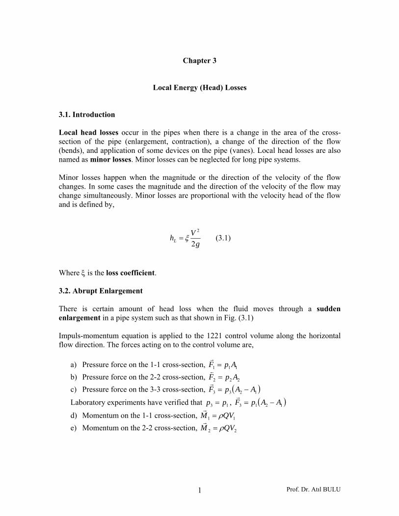
Where ξ is the loss coefficient. 3.2. Abrupt Enlargement There is certain amount of head loss when the fluid moves through a sudden enlargement in a pipe system such as that shown in Fig. (3.1) Impuls-momentum equation is applied to the 1221 control volume along the horizontal flow direction. The forces acting on to the control volume are,
a) Pressure force on the 1-1 cross-section, 111 ApF =r
b) Pressure force on the 2-2 cross-section, 222 ApF =
s
c) Pressure force on the 3-3 cross-section, ( )1233 AApF −=r
Laboratory experiments have verified that 13 pp = , ( )1213 AApF −=r
d) Momentum on the 1-1 cross-section, 11 QVM ρ=r
e) Momentum on the 2-2 cross-section, 22 QVM ρ=
r
Prof. Dr. Atıl BULU 2
Fig. 3.1.
Neglecting the shearing force on the surface of the control volume,
( )( ) ( )
( )122
21
12221
222121111 0
VVgAQpp
g
VVQAppQVApAApApQV
−=−
=
−=−=−−−++
γ
γρ
ρρρ
p1A1 ρQV1
p2A2 ρQV2
p1(A2 -A1)
1
3 2
23
Energy Line
( )gVV
hL 2
221 −=
gV2
21
γ1p
1
gV2
22
γ2p
Flow
3 2
H.G.L
Prof. Dr. Atıl BULU 3
Applying the continuity equation,
2
112
2211
AAVV
AVAVQ
=
==
Substituting this,
⎟⎟⎠
⎞⎜⎜⎝
⎛−=
−111
2
1111
2
21 1 VAVAAVAV
gApp
γ
⎥⎥⎦
⎤
⎢⎢⎣
⎡−⎟⎟
⎠
⎞⎜⎜⎝
⎛=
−
2
1
2
2
12
121
AA
AA
gVpp
γ (3.2)
Applying Bernoulli equation between cross-sections 1-2 for the horizontal pipe flow,
L
L
hg
Vg
Vpp
hg
Vpg
Vp
+−=−
++=+
22
222
12
221
222
211
γ
γγ
Substituting Equ. (3.2),
gV
gVV
gVh
gVV
gV
gV
gVh
VV
VV
gV
gV
gVh
VV
AAAVAV
hg
Vg
VAA
AA
gV
L
L
L
L
22
22
22
222
2221
21
212
22
22
1
1
2
2
1
22
12
22
1
1
2
2
12211
21
22
2
1
2
2
12
1
+−=
−+−=
⎥⎥⎦
⎤
⎢⎢⎣
⎡−⎟⎟
⎠
⎞⎜⎜⎝
⎛+−=
=→=
+−=⎥⎥⎦
⎤
⎢⎢⎣
⎡−⎟⎟
⎠
⎞⎜⎜⎝
⎛
Prof. Dr. Atıl BULU 4
( )gVVhL 2
221 −= (3.3)
This equation is known as Borda-Carnot equation. The loss coefficient can be derived as,
⎟⎟⎠
⎞⎜⎜⎝
⎛+−=
⎟⎟⎠
⎞⎜⎜⎝
⎛+−=
22
21
2
12
1
21
22
1
22
1
212
212
AA
AA
gVh
VV
VV
gVh
L
L
2
2
12
1 12 ⎟⎟
⎠
⎞⎜⎜⎝
⎛−=
AA
gVhL (3.4)
The loss coefficient of Equ. (3.1) is then,
2
2
11 ⎟⎟⎠
⎞⎜⎜⎝
⎛−=
AAξ (3.5)
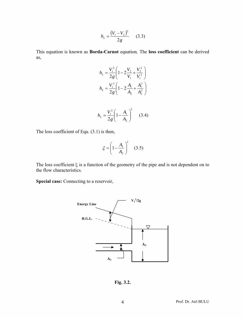
The loss coefficient ξ is a function of the geometry of the pipe and is not dependent on to the flow characteristics. Special case: Connecting to a reservoir,
Fig. 3.2.
A2
A1
V12/2g
Energy Line
H.G.L.
Prof. Dr. Atıl BULU 5
1 a
2
1 a
2
A1 A2V1 V2pa
Dead Zone
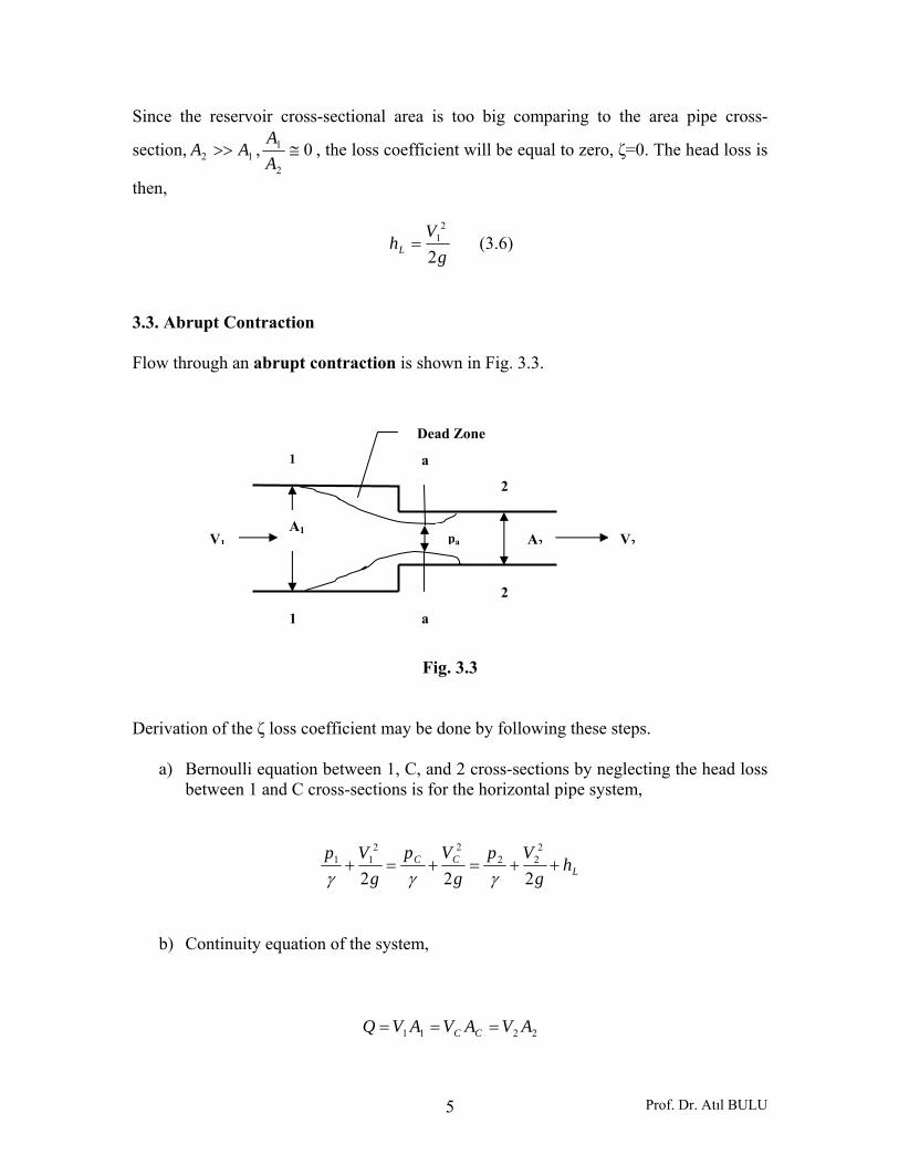
Since the reservoir cross-sectional area is too big comparing to the area pipe cross-
section, 12 AA >> , 02
1 ≅AA
, the loss coefficient will be equal to zero, ζ=0. The head loss is
then,
gV
hL 2
21= (3.6)
3.3. Abrupt Contraction Flow through an abrupt contraction is shown in Fig. 3.3.
Fig. 3.3
Derivation of the ζ loss coefficient may be done by following these steps.
a) Bernoulli equation between 1, C, and 2 cross-sections by neglecting the head loss between 1 and C cross-sections is for the horizontal pipe system,
LCC h
gVp
gVp
gVp
++=+=+222
222
2211
γγγ
b) Continuity equation of the system,
2211 AVAVAVQ CC ===
Prof. Dr. Atıl BULU 6
c) Impuls-Momentum equation between C and 2 cross-sections,
( ) ( )CC VVQApp −=− 222 ρ
Solving these 3 equations gives us head loss equation as,
( )
gV
AA
h
gVV
h
CL
CL
21
22
22
2
22
⎟⎟⎠
⎞⎜⎜⎝
⎛−=
−=
(3.7)
Where,
2AA
C CC = = Coefficient of contraction (3.8)
The loss coefficient for abrupt contraction is then,
2
11⎟⎟⎠
⎞⎜⎜⎝
⎛−=
CCξ (3.9)
gV
hL 2
22ξ=
CC contraction coefficients, and ζ loss coefficients have determined by laboratory experiments depending on the A2/A1 ratios and given in Table 3.1.
Prof. Dr. Atıl BULU 7
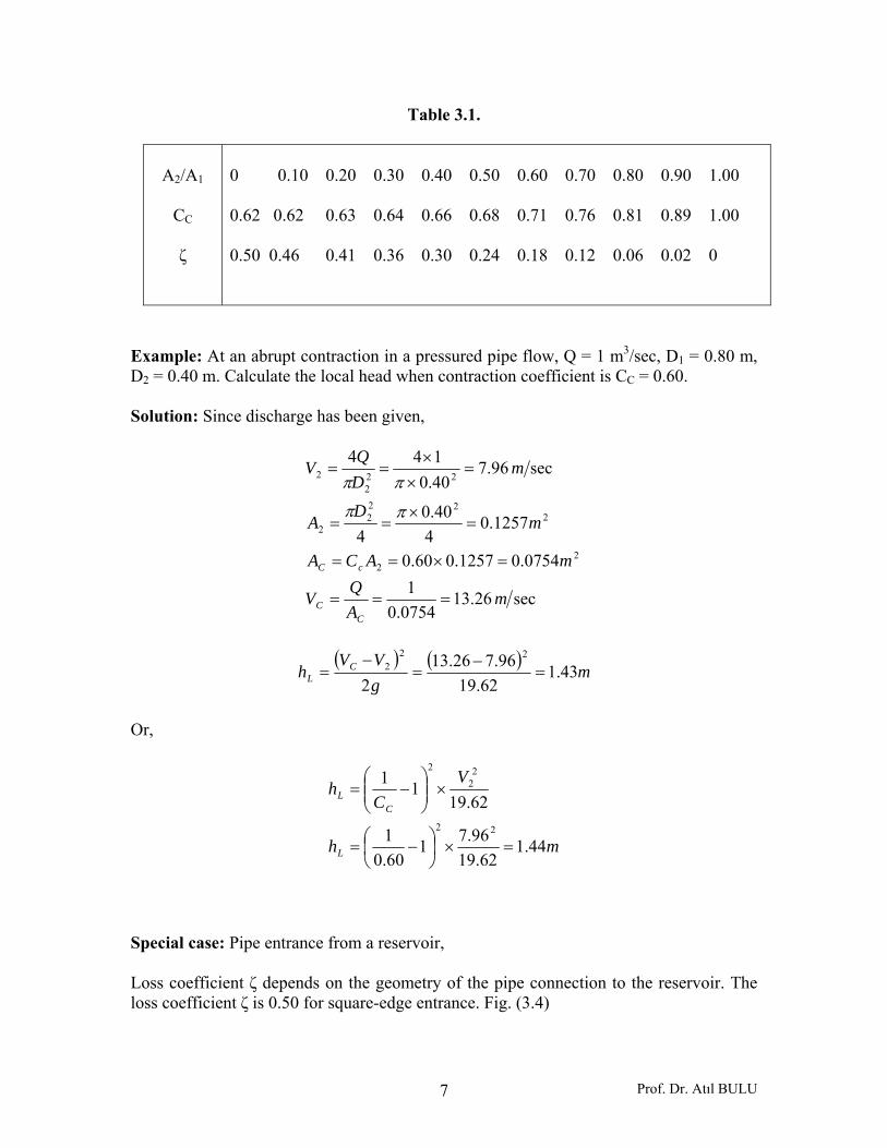
Table 3.1.
A2/A1
CC
ζ
0 0.10 0.20 0.30 0.40 0.50 0.60 0.70 0.80 0.90 1.00 0.62 0.62 0.63 0.64 0.66 0.68 0.71 0.76 0.81 0.89 1.00 0.50 0.46 0.41 0.36 0.30 0.24 0.18 0.12 0.06 0.02 0
Example: At an abrupt contraction in a pressured pipe flow, Q = 1 m3/sec, D1 = 0.80 m, D2 = 0.40 m. Calculate the local head when contraction coefficient is CC = 0.60. Solution: Since discharge has been given,
sec26.130754.01
0754.01257.060.0
1257.04
40.04
sec96.740.0144
22
222
22
222
2
mAQV
mACA
mD
A
mDQV
CC
cC
===
=×==
=×
==
=××
==
ππ
ππ
( ) ( ) m
gVV
h CL 43.1
62.1996.726.13
2
222 =
−=
−=
Or,
mh
VC
h
L
CL
44.162.19
96.7160.01
62.1911
22
22
2
=×⎟⎠⎞
⎜⎝⎛ −=
×⎟⎟⎠
⎞⎜⎜⎝
⎛−=
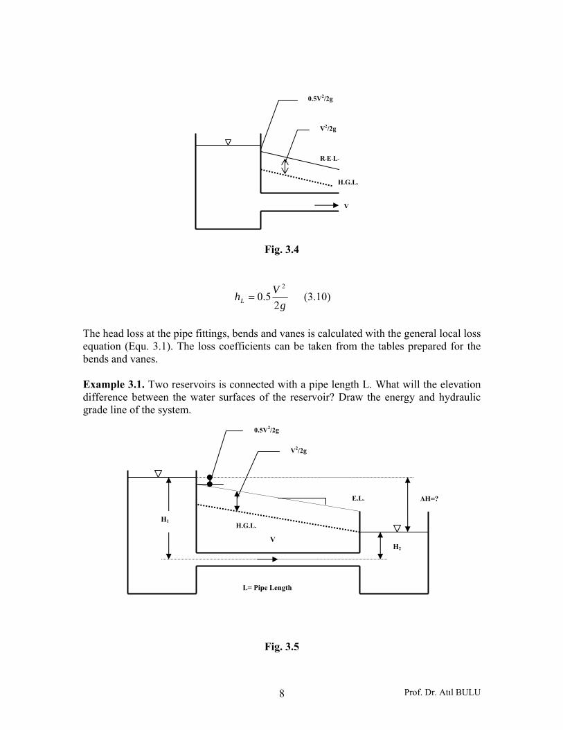
Special case: Pipe entrance from a reservoir, Loss coefficient ζ depends on the geometry of the pipe connection to the reservoir. The loss coefficient ζ is 0.50 for square-edge entrance. Fig. (3.4)
Prof. Dr. Atıl BULU 8
Fig. 3.4
gVhL 2
5.02
= (3.10)
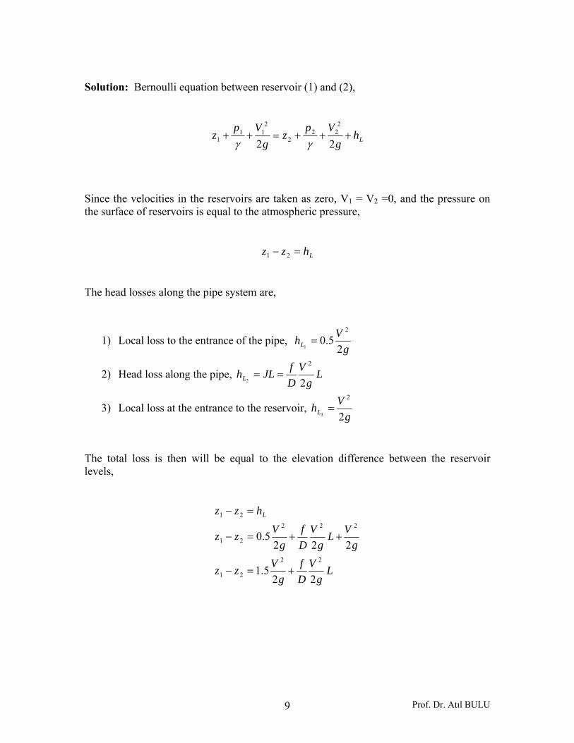
The head loss at the pipe fittings, bends and vanes is calculated with the general local loss equation (Equ. 3.1). The loss coefficients can be taken from the tables prepared for the bends and vanes. Example 3.1. Two reservoirs is connected with a pipe length L. What will the elevation difference between the water surfaces of the reservoir? Draw the energy and hydraulic grade line of the system.
Fig. 3.5
H1
H2
ΔH=?
V2/2g
0.5V2/2g
E.L.
H.G.L.
V
L= Pipe Length
V2/2g
0.5V2/2g
R.E.L.
H.G.L.
V
Prof. Dr. Atıl BULU 9
Solution: Bernoulli equation between reservoir (1) and (2),
Lhg
Vpz
gVp
z +++=++22
222
2
211
1 γγ
Since the velocities in the reservoirs are taken as zero, V1 = V2 =0, and the pressure on the surface of reservoirs is equal to the atmospheric pressure,
Lhzz =− 21
The head losses along the pipe system are,
1) Local loss to the entrance of the pipe, g
VhL 25.0
2
1=
2) Head loss along the pipe, Lg
VDfJLhL 2
2
2==
3) Local loss at the entrance to the reservoir, g
VhL 2
2
3=
The total loss is then will be equal to the elevation difference between the reservoir levels,
Lg
VDf
gVzz
gVL
gV
Df
gVzz
hzz L
225.1
2225.0
22
21
222
21
21
+=−
++=−
=−
Prof. Dr. Atıl BULU 10
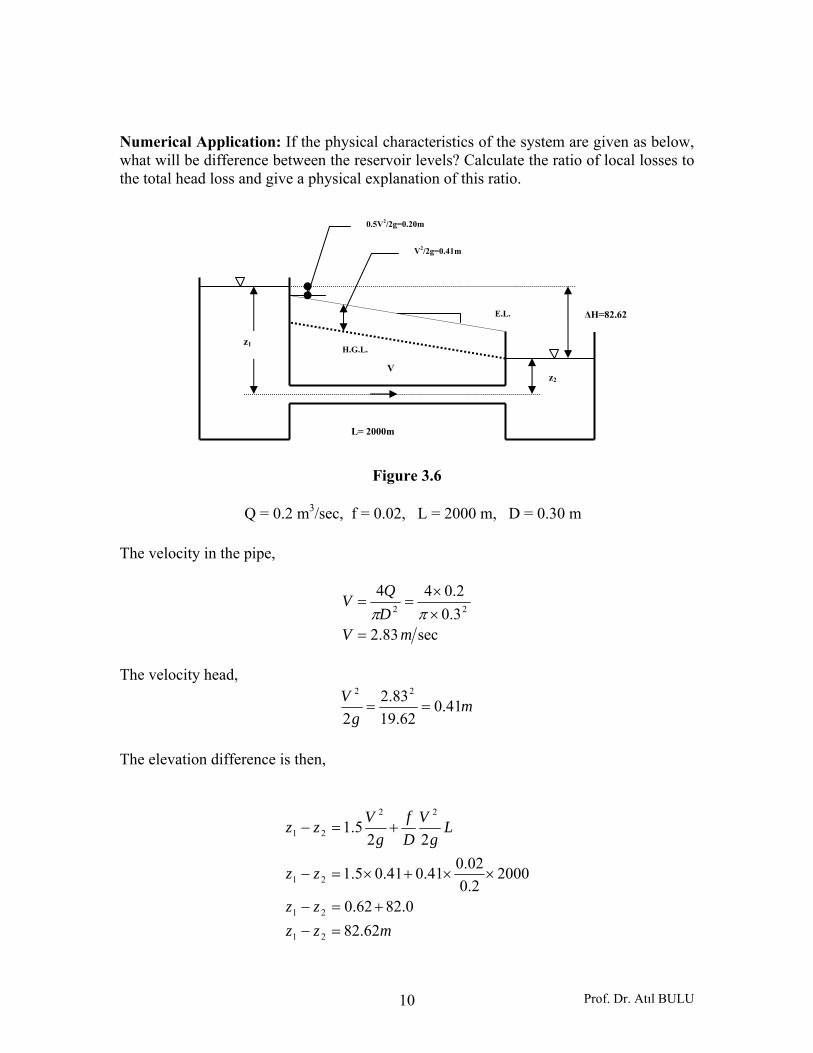
Numerical Application: If the physical characteristics of the system are given as below, what will be difference between the reservoir levels? Calculate the ratio of local losses to the total head loss and give a physical explanation of this ratio.
Figure 3.6
Q = 0.2 m3/sec, f = 0.02, L = 2000 m, D = 0.30 m
The velocity in the pipe,
sec83.23.02.044
22
mVDQV
=××
==ππ
The velocity head,
mg
V 41.062.19
83.22
22
==
The elevation difference is then,
mzzzz
zz
Lg
VDf
gVzz
62.820.8262.0
20002.002.041.041.05.1
225.1
21
21
21
22
21
=−+=−
××+×=−
+=−
z1
z2
ΔH=82.62
V2/2g=0.41m
0.5V2/2g=0.20m
E.L.
H.G.L.
V
L= 2000m
Prof. Dr. Atıl BULU 11
The ratio of local losses to the total head loss is,
0075.062.8262.0
=
As can be seen from the result, the ratio is less than 1%. Therefore, local losses are generally neglected for long pipes. 3.4 Conduit Systems The other applications which are commonly seen in practical applications for conduit systems are,
a) The Three-Reservoir Problems, b) Parallel Pipes, c) Branching Pipes, d) Pump Systems.
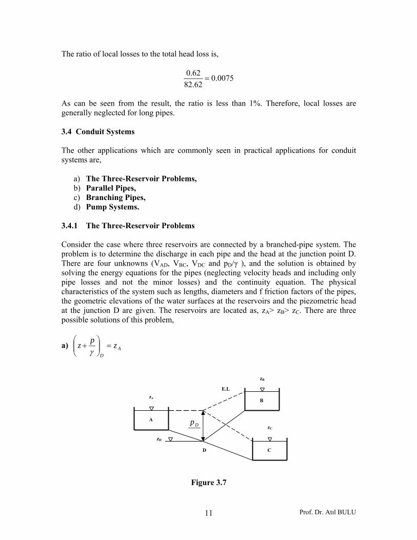
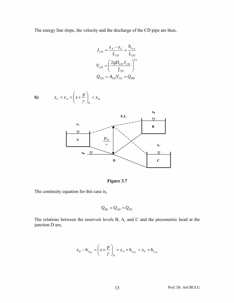
3.4.1 The Three-Reservoir Problems Consider the case where three reservoirs are connected by a branched-pipe system. The problem is to determine the discharge in each pipe and the head at the junction point D. There are four unknowns (VAD, VBC, VDC and pD/γ ), and the solution is obtained by solving the energy equations for the pipes (neglecting velocity heads and including only pipe losses and not the minor losses) and the continuity equation. The physical characteristics of the system such as lengths, diameters and f friction factors of the pipes, the geometric elevations of the water surfaces at the reservoirs and the piezometric head at the junction D are given. The reservoirs are located as, zA> zB> zC. There are three possible solutions of this problem,
a) AD
zpz =⎟⎟⎠
⎞⎜⎜⎝
⎛+γ
Figure 3.7
A
zA
zB
zC
B
C
Dp
D
zD
E.L
Prof. Dr. Atıl BULU 12
Since AD
zpz =⎟⎟⎠
⎞⎜⎜⎝
⎛+γ
, there will be no flow from or to reservoir A, and therefore,
0,0,0 === ADADAD JVQ
DCBD QQ =
The relations between the reservoir levels B, and D and the piezometric head at the junction D are,
CDBD LCD
DLB hzp
zhz +=+=−γ
Energy line slope (JBD) of the BD pipe can be found as,
BD
L
BD
AB
BD
DDB
BD Lh
Lzz
L
pzz
J BD=−
=−−
=γ (3.11)
Using the Darcy-Weisbach equation,
gDfVJ
2
2
=
The flow velocity in the BD pipe can be calculated by,
212
⎟⎟⎠
⎞⎜⎜⎝
⎛=
BD
BDBDBD f
JgDV (3.12)
And the discharge is,
BDBDBD VAQ =
Prof. Dr. Atıl BULU 13
The energy line slope, the velocity and the discharge of the CD pipe are then,
BDCdCDCD
CD
CDCDCD
CD
L
CD
CACD
QVAQf
JgDV
Lh
Lzz
J CD
==
⎟⎟⎠
⎞⎜⎜⎝
⎛=
=−
=
212
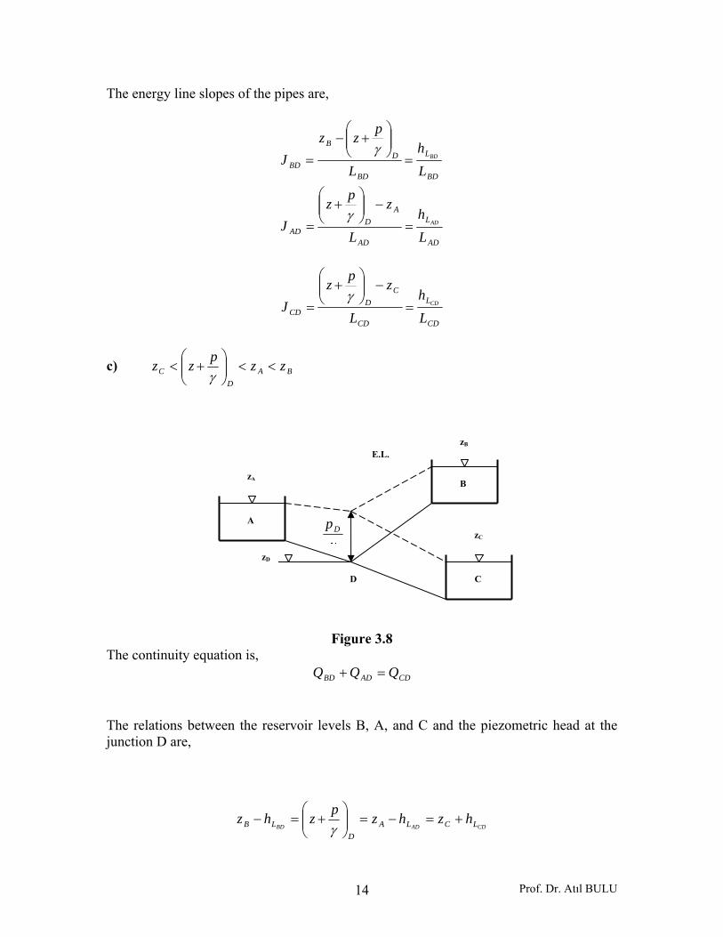
b) BD
AC zpzzz <⎟⎟⎠
⎞⎜⎜⎝
⎛+<<γ
Figure 3.7
The continuity equation for this case is,
DCADBd QQQ += The relations between the reservoir levels B, A, and C and the piezometric head at the junction D are,
CDADBD LCLAD
LB hzhzpzhz +=+=⎟⎟⎠
⎞⎜⎜⎝
⎛+=−γ
A
zA
zB
zC
B
C
γDp
D
zD
E.L.
Prof. Dr. Atıl BULU 14
The energy line slopes of the pipes are,
AD
L
AD
AD
AD
BD
L
BD
DB
BD
Lh
L
zpzJ
Lh
L
pzzJ
AD
BD
=
−⎟⎟⎠
⎞⎜⎜⎝
⎛+
=
=⎟⎟⎠
⎞⎜⎜⎝
⎛+−
=
γ
γ
CD
L
CD
CD
CD Lh
L
zpzJ CD=
−⎟⎟⎠
⎞⎜⎜⎝
⎛+
=γ
c) BAD
C zzpzz <<⎟⎟⎠
⎞⎜⎜⎝
⎛+<γ
Figure 3.8 The continuity equation is,
CDADBD QQQ =+
The relations between the reservoir levels B, A, and C and the piezometric head at the junction D are,
CDADBD LCLAD
LB hzhzpzhz +=−=⎟⎟⎠
⎞⎜⎜⎝
⎛+=−γ
A
zA
zB
zC
B
C
γDp
D
zD
E.L.
Prof. Dr. Atıl BULU 15
The energy line slopes of the pipes are,
CD
L
CD
CD
CD
AD
L
AD
DA
AD
BD
L
BD
DB
BD
Lh
L
zpzJ
Lh
L
pzzJ
Lh
L
pzzJ
CD
AD
BD
=
−⎟⎟⎠
⎞⎜⎜⎝
⎛+
=
=⎟⎟⎠
⎞⎜⎜⎝
⎛+−
=
=⎟⎟⎠
⎞⎜⎜⎝
⎛+−
=
γ
γ
γ
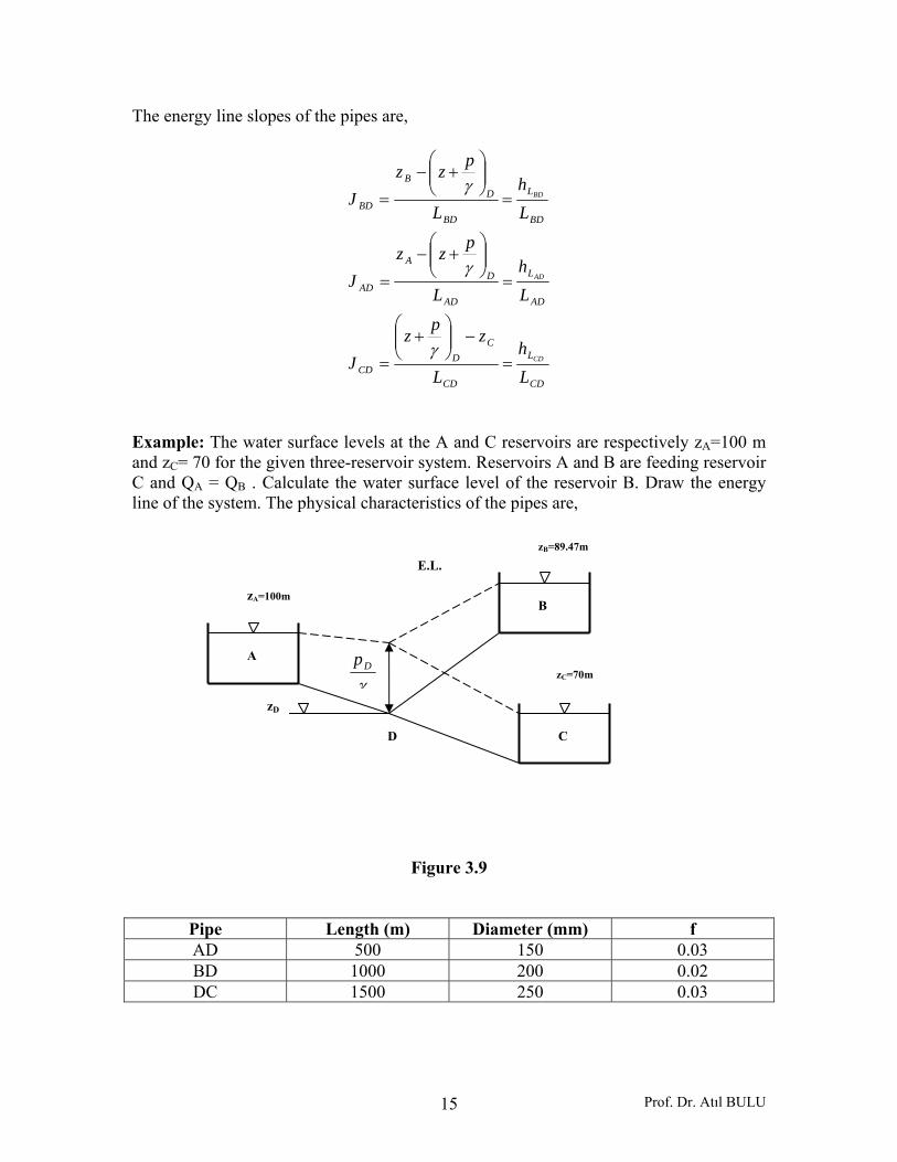
Example: The water surface levels at the A and C reservoirs are respectively zA=100 m and zC= 70 for the given three-reservoir system. Reservoirs A and B are feeding reservoir C and QA = QB . Calculate the water surface level of the reservoir B. Draw the energy line of the system. The physical characteristics of the pipes are,
Figure 3.9
Pipe Length (m) Diameter (mm) f AD 500 150 0.03 BD 1000 200 0.02 DC 1500 250 0.03
A
zA=100m
zB=89.47m
zC=70m
B
C
γDp
D
zD
E.L.
Prof. Dr. Atıl BULU 16
Solution: The head loss along the pipes 1 and 3 is,
mzzhh CALL 307010031
=−=−=+ (1)
Since,
QQQQQ
23
21
===
Using the Darcy-Weisbach equation for the head loss,
5
2
2
2
2
2
8
422
DLQ
gfh
DQ
gfL
gDLfVh
L
L
×=
⎟⎠⎞
⎜⎝⎛×==
π
π
Using Equ. (1),
( )
sec8.30sec0308.03156630
25.021500
15.0500
81.903.0830
8
3
2
5
2
5
2
2
52
2222
51
2111
2
ltmQQ
DQLf
DQLf
ghL
==
=
⎥⎦
⎤⎢⎣
⎡ ×+
××
×=
⎟⎟⎠
⎞⎜⎜⎝
⎛+=
π
π
sec74.115.0
0308.044sec0308.0
221
11
31
mDQ
V
mQ
=××
==
=
ππ
sec26.125.0
0616.044sec0616.00308.022
223
33
313
mDQ
V
mQQ
=××
==
=×==
ππ
Prof. Dr. Atıl BULU 17
Head losses along the pipes are,
mhh
mgD
LVfh
mgD
LVfh
Ll
L
L
00.3057.1443.15
57.1425.062.19150026.103.0
2
43.1515.062.19
50074.103.02
31
3
1
2
3
32
33
2
1
12
11
=+=+
=×
××==
=×
××==
For the pipe 2,
sec0308.0 321 mQQ ==
mgD
LVfh
mDQ
V
L 90.420.062.19100098.002.0
2
sec98.020.0
0308.044
2
2
22
22
222
22
2=
×××
==
=××
==ππ
Water surface level of the reservoir B is,
mhpzz
mhzpz
mhzpz
LD
B
LCD
LAD
47.8990.457.84
57.8457.1400.70
57.8443.1500.100
2
3
1
=+=+⎟⎟⎠
⎞⎜⎜⎝
⎛+=
=+=+=⎟⎟⎠
⎞⎜⎜⎝
⎛+
=−=−=⎟⎟⎠
⎞⎜⎜⎝
⎛+
γ
γ
γ
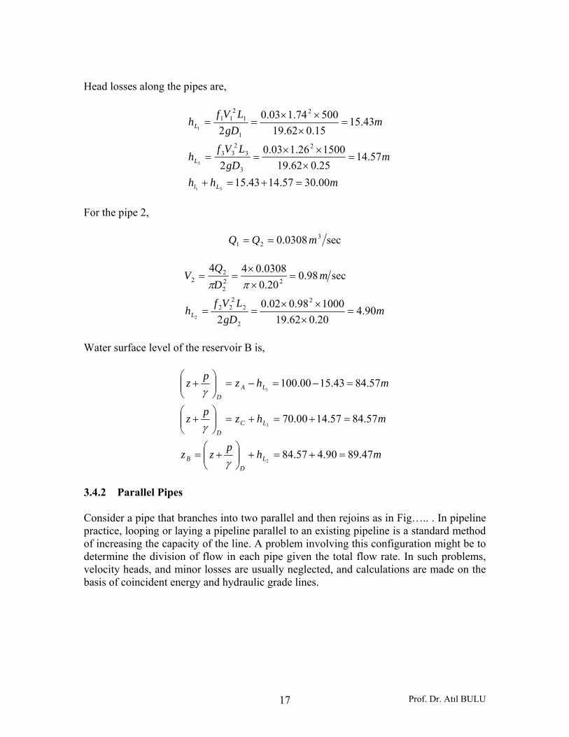
3.4.2 Parallel Pipes Consider a pipe that branches into two parallel and then rejoins as in Fig….. . In pipeline practice, looping or laying a pipeline parallel to an existing pipeline is a standard method of increasing the capacity of the line. A problem involving this configuration might be to determine the division of flow in each pipe given the total flow rate. In such problems, velocity heads, and minor losses are usually neglected, and calculations are made on the basis of coincident energy and hydraulic grade lines.
Prof. Dr. Atıl BULU 18
Figure 3.10
Evidently, the distribution of flow in the branches must be such that the same head loss occurs in each branch; if this were not so there would be more than one energy line for the pipe upstream and downstream from the junctions. Application of the continuity principle shows that the discharge in the mainline is equal to the sum of the discharges in the branches. Thus the following simultaneous equations may be written.
21
21
QQQ
hh LL
+=
= (3.13)
Using the equality of head losses,
gDVLf
gDVLf
22 2
2222
1
2111 =
21
211
122
2
1⎟⎟⎠
⎞⎜⎜⎝
⎛=
DLfDLf
VV
(3.14)
If f1 and f2 are known, the division of flow can be easily determined.
Q1, L1, D1, f1
Q2, L2, D2, f2
Q Q
A B
hL1 = hL2
PB/γ
PA/γ
E.L
Prof. Dr. Atıl BULU 19
Expressing the head losses in terms of discharge through the Darcy-Weisbach equation,
42
22 1622 D
QgDfL
gDLfVhL π
×=
2
2522
16
KQh
QgDfLh
L
L
=
×⎟⎟⎠
⎞⎜⎜⎝
⎛=
π (3.14)
Substituting this to the simultaneous Equs (3.12),
21
222
211
QQQQKQK
+==
(3.15)
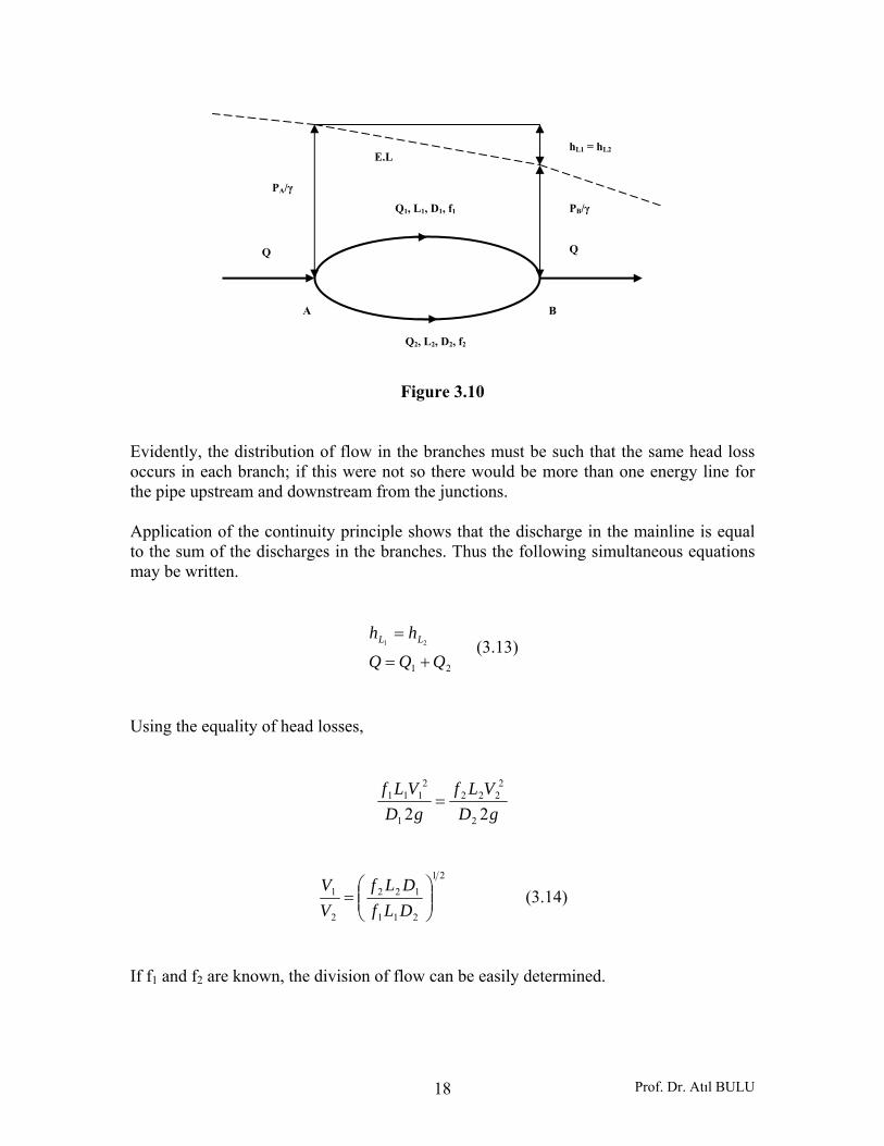
Solution of these simultaneous equations allows prediction of the division of a discharge Q into discharges Q1 and Q2 when the pipe characteristics are known. Application of these principles allows prediction of the increased discharge obtainable by looping an existing pipeline. Example: A 300 mm pipeline 1500 m long is laid between two reservoirs having a difference of surface elevation of 24. The maximum discharge obtainable through this line is 0.15m3/sec. When this pipe is looped with a 600 m pipe of the same size and material laid parallel and connected to it, what increase of discharge may be expected? Solution: For the single pipe, using Equ. (3.14),
106715.024 2
2
=×=
=
KK
KQhL
Prof. Dr. Atıl BULU 20
Figure 3.11
K for the looped section is,
427
106715006002
=
×==
A
A
K
KLL
K
For the unlooped section,
640
10671500
6001500
2
=′
×−
=′
−=′
K
K
KLLL
K
For the looped pipeline, the headloss is computed first in the common section plus branch A as,
22
22
42764024 A
AAL
QKQKh
×+×=
+′= (1)
And then in the common section plus branch B as,
22 42764024 BQQ ×+×= (2)
24m 1
1A
B, LB=600m
Prof. Dr. Atıl BULU 21
In which QA and QB are the discharges in the parallel branches. Solving these by eliminating Q shows that QA=QB (which is expected to be from symmetry in this problem). Since, from continuity,
2QQ
QQQ
A
BA
=
+=
Substituting this in the Equ (1) yields,
( )
sec18.0sec09.0
298724
427264024
3
3
2
22
mQmQ
Q
A
A
AA
=
=
=
×+×=
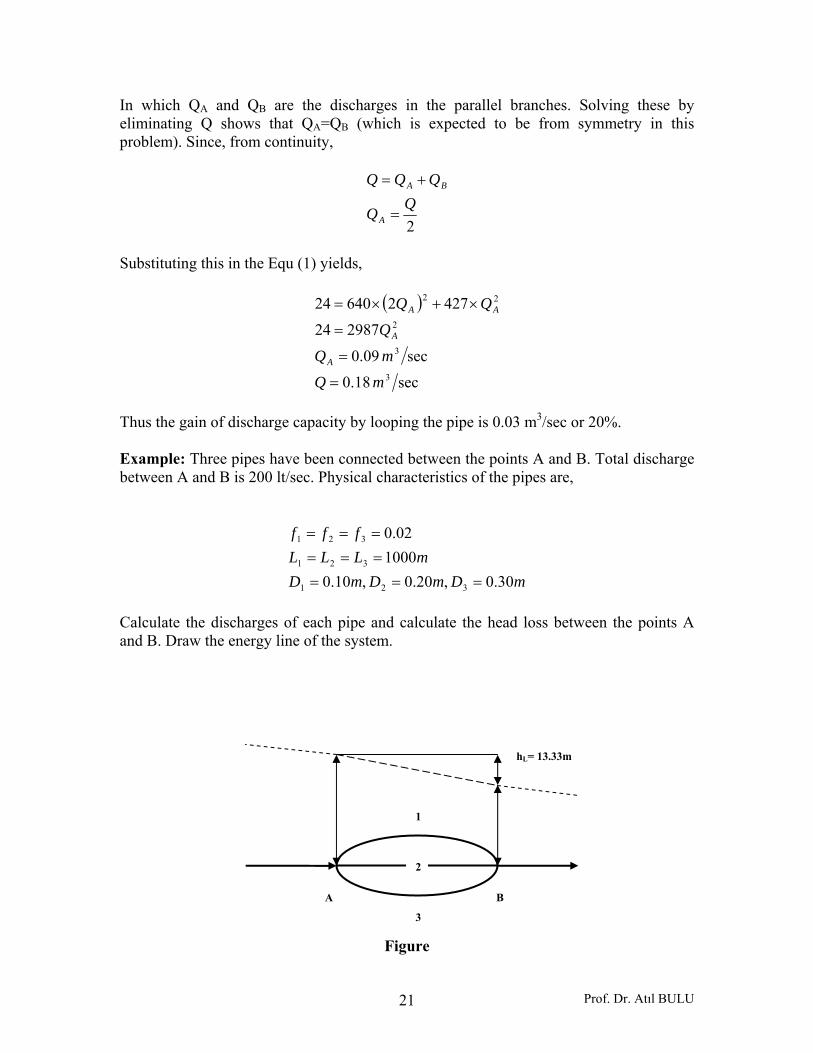
Thus the gain of discharge capacity by looping the pipe is 0.03 m3/sec or 20%. Example: Three pipes have been connected between the points A and B. Total discharge between A and B is 200 lt/sec. Physical characteristics of the pipes are,
mDmDmDmLLL
fff
30.0,20.0,10.01000
02.0
321
321
321
=========
Calculate the discharges of each pipe and calculate the head loss between the points A and B. Draw the energy line of the system.
Figure
A B
1
2
3
hL= 13.33m
Prof. Dr. Atıl BULU 22
Solution: Head losses through the three pipes should be the same.
321 LLL hhh ==
332211 LJLJLJ ==
Since the pipe lengths are the same for the three pipes,
321 JJJ ==
5
2
242
22 81621
2 DQ
gf
DQ
gDf
gV
DfJ ×=××=×=
ππ
And also roughness coefficients f are the same for three pipe, the above equation takes the form of,
53
23
52
22
51
21
DQ
DQ
DQ
==
Using this equation,
21
5.225
2
1
2
1
177.0
177.020.010.0
QQDD
=
=⎟⎠⎞
⎜⎝⎛=⎟⎟
⎠
⎞⎜⎜⎝
⎛=
23
5.225
2
3
2
3
76.2
76.220.030.0
QQDD
=
=⎟⎠⎞
⎜⎝⎛=⎟⎟
⎠
⎞⎜⎜⎝
⎛=
Substituting these values to the continuity equation,
sec051.0
200.0937.3200.076.2177.0
200.0
32
2
222
321
mQ
QQQQ
QQQ
=
==++
=++
sec140.0051.076.2
sec009.0051.0177.03
3
31
mQ
mQ
=×=
=×=
sec200.0140.0051.0009.0 3
321 mQQQ =++=++
Prof. Dr. Atıl BULU 23
Calculated discharges for the parallel pipes satisfy the continuity equation. The head loss for the parallel pipes is,
mh
LDQ
gfh
AB
AB
L
L
33.13100030.014.0
81.902.08
8
5
2
2
353
23
2
=×××
×=
××=
π
π
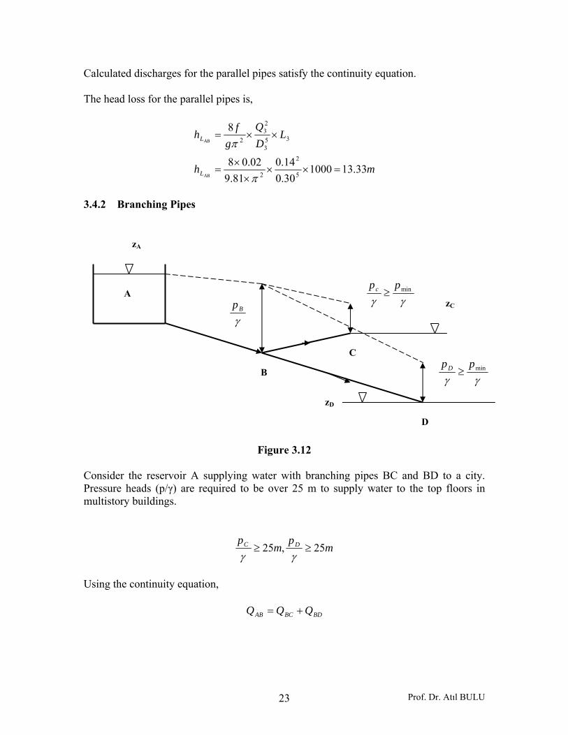
3.4.2 Branching Pipes
Figure 3.12
Consider the reservoir A supplying water with branching pipes BC and BD to a city. Pressure heads (p/γ) are required to be over 25 m to supply water to the top floors in multistory buildings.
mp
mp DC 25,25 ≥≥
γγ
Using the continuity equation,
BDBCAB QQQ +=
A
zA
B
C
D
γγminppc ≥
γγminppD ≥
zC
zD
γBp
Prof. Dr. Atıl BULU 24
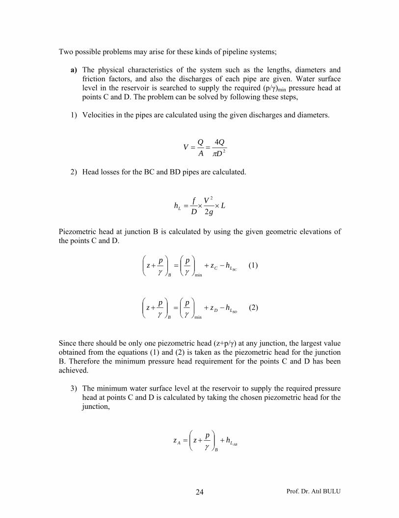
Two possible problems may arise for these kinds of pipeline systems;
a) The physical characteristics of the system such as the lengths, diameters and friction factors, and also the discharges of each pipe are given. Water surface level in the reservoir is searched to supply the required (p/γ)min pressure head at points C and D. The problem can be solved by following these steps,
1) Velocities in the pipes are calculated using the given discharges and diameters.
2
4DQ
AQV
π==
2) Head losses for the BC and BD pipes are calculated.
Lg
VDfhL ××=
2
2
Piezometric head at junction B is calculated by using the given geometric elevations of the points C and D.
BCLCB
hzppz −+⎟⎟⎠
⎞⎜⎜⎝
⎛=⎟⎟
⎠
⎞⎜⎜⎝
⎛+
minγγ (1)
BDLDB
hzppz −+⎟⎟⎠
⎞⎜⎜⎝
⎛=⎟⎟
⎠
⎞⎜⎜⎝
⎛+
minγγ (2)
Since there should be only one piezometric head (z+p/γ) at any junction, the largest value obtained from the equations (1) and (2) is taken as the piezometric head for the junction B. Therefore the minimum pressure head requirement for the points C and D has been achieved.
3) The minimum water surface level at the reservoir to supply the required pressure head at points C and D is calculated by taking the chosen piezometric head for the junction,
ABLB
A hpzz +⎟⎟⎠
⎞⎜⎜⎝
⎛+=γ
Prof. Dr. Atıl BULU 25
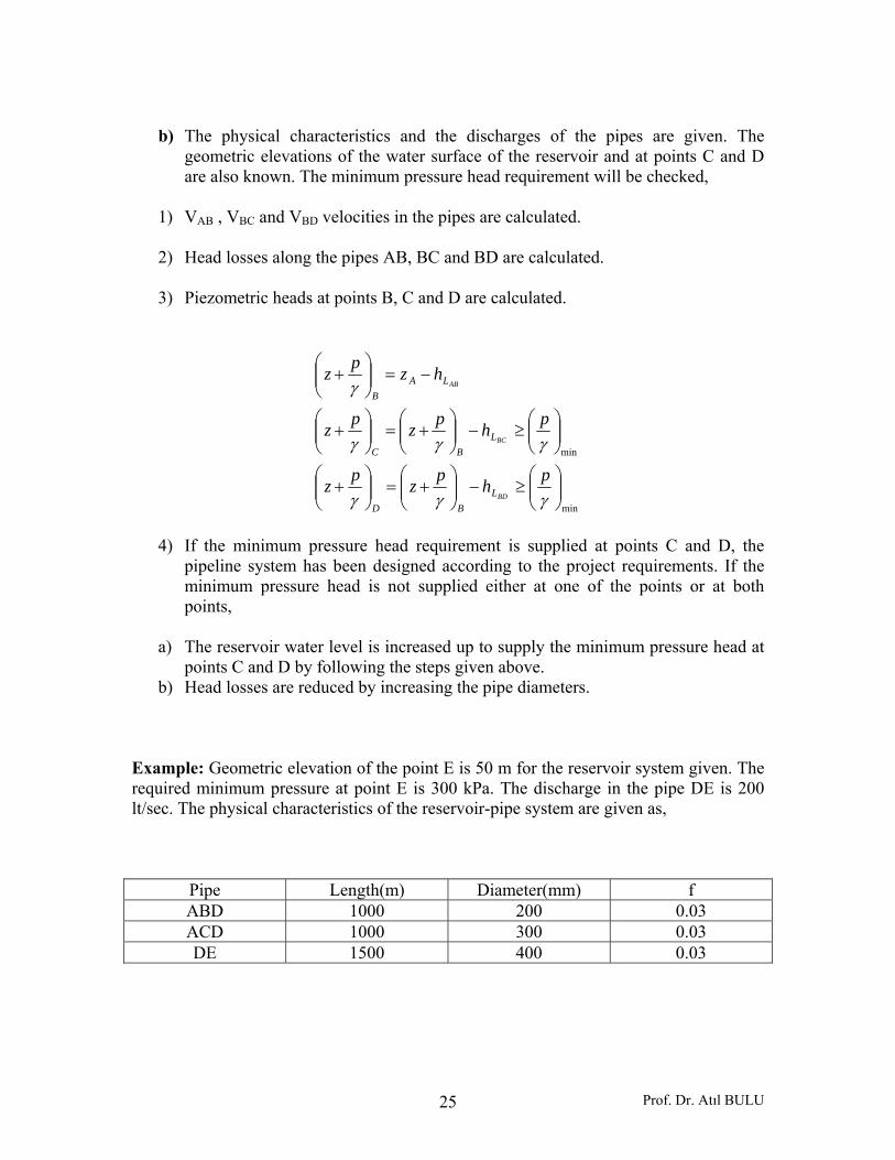
b) The physical characteristics and the discharges of the pipes are given. The
geometric elevations of the water surface of the reservoir and at points C and D are also known. The minimum pressure head requirement will be checked,
1) VAB , VBC and VBD velocities in the pipes are calculated. 2) Head losses along the pipes AB, BC and BD are calculated.
3) Piezometric heads at points B, C and D are calculated.
min
min
⎟⎟⎠
⎞⎜⎜⎝
⎛≥−⎟⎟
⎠
⎞⎜⎜⎝
⎛+=⎟⎟
⎠
⎞⎜⎜⎝
⎛+
⎟⎟⎠
⎞⎜⎜⎝
⎛≥−⎟⎟
⎠
⎞⎜⎜⎝
⎛+=⎟⎟
⎠
⎞⎜⎜⎝
⎛+
−=⎟⎟⎠
⎞⎜⎜⎝
⎛+
γγγ
γγγ
γ
phpzpz
phpzpz
hzpz
BD
BC
AB
LBD
LBC
LAB
4) If the minimum pressure head requirement is supplied at points C and D, the
pipeline system has been designed according to the project requirements. If the minimum pressure head is not supplied either at one of the points or at both points,
a) The reservoir water level is increased up to supply the minimum pressure head at
points C and D by following the steps given above. b) Head losses are reduced by increasing the pipe diameters.
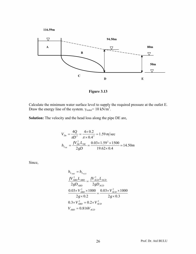
Example: Geometric elevation of the point E is 50 m for the reservoir system given. The required minimum pressure at point E is 300 kPa. The discharge in the pipe DE is 200 lt/sec. The physical characteristics of the reservoir-pipe system are given as,
Pipe Length(m) Diameter(mm) f ABD 1000 200 0.03 ACD 1000 300 0.03 DE 1500 400 0.03
Prof. Dr. Atıl BULU 26
Figure 3.13
Calculate the minimum water surface level to supply the required pressure at the outlet E. Draw the energy line of the system. γwater= 10 kN/m3. Solution: The velocity and the head loss along the pipe DE are,
mgD
LfVh
mDQV
DEDEL
De
DE50.14
4.062.19150059.103.0
2
sec59.14.02.044
22
22
=×××
==
=××
==ππ
Since,
ACDABD
ACDABD
ACDABD
ACD
ACDACD
ABD
ABDABD
LL
VVVV
gV
gV
gDLfV
gDLfV
hhACDABD
816.02.03.0
3.02100003.0
2.02100003.0
22
22
22
22
=×=×
×××
=×
××
=
=
A
B
CD E
50m
80m
94.50m
116.59m
Prof. Dr. Atıl BULU 27
Applying the continuity equation,
( )
sec70.108.2816.0sec08.2
255.009.0816.004.0255.009.004.0
200.03.02.04
222
mVmV
VVVV
VV
QQQ
ABD
ACD
ACDACD
ACDABD
ACDABD
ACDABD
=×==
=×+××=×+×
=×+××
+=π
The discharges of the looped pipes are,
sec053.0
70.14
2.04
3
2
2
mQ
Q
VD
Q
ABD
ABD
ABDABD
ABD
=
××
=
×=
π
π
sec147.0
08.24
3.04
3
2
2
mQ
Q
VD
Q
ACD
ACD
ACDACD
ACD
=
××
=
××
=
π
π
The head loss along the looped pipes is,
mh
h
gDLfV
hh
L
L
ABD
ABDABDLL ABDACD
09.222.062.19100070.103.0
22
2
=×××
=
==
Prof. Dr. Atıl BULU 28
Piezometric head at the outlet E is,
mpzEw
801030050 =+=⎟⎟
⎠
⎞⎜⎜⎝
⎛+γ
The required minimum water surface level at the reservoir is,
ACDDe LLE
A hhpzz ++⎟⎟⎠
⎞⎜⎜⎝
⎛+=γ
mzz
A
A
59.11609.2250.1480
=++=
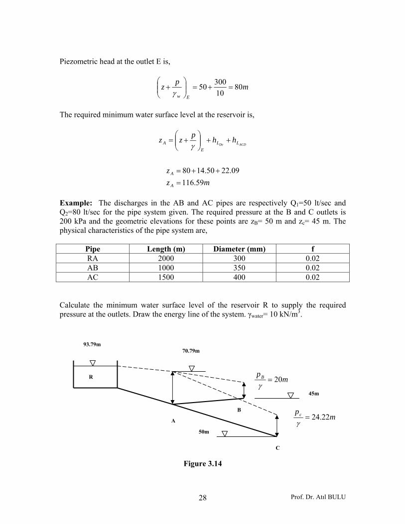
Example: The discharges in the AB and AC pipes are respectively Q1=50 lt/sec and Q2=80 lt/sec for the pipe system given. The required pressure at the B and C outlets is 200 kPa and the geometric elevations for these points are zB= 50 m and zc= 45 m. The physical characteristics of the pipe system are,
Pipe Length (m) Diameter (mm) f RA 2000 300 0.02 AB 1000 350 0.02 AC 1500 400 0.02
Calculate the minimum water surface level of the reservoir R to supply the required pressure at the outlets. Draw the energy line of the system. γwater= 10 kN/m3.
Figure 3.14
A
B
C
R
70.79m
mpc 22.24=γ
50m
mpB 20=γ
45m
93.79m
Prof. Dr. Atıl BULU 29
Solution: Since the discharges in the pipes are given,
mgD
LfVh
mDQ
V
AB
ABABL
AB
ABAB
AB79.0
35.062.19100052.002.0
2
sec52.035.0050.044
22
22
=×
××==
=××
==ππ
ABLBA
hpzpz +⎟⎟⎠
⎞⎜⎜⎝
⎛+=⎟⎟
⎠
⎞⎜⎜⎝
⎛+
γγ
mpzA
79.7079.01020050 =+⎟
⎠⎞
⎜⎝⎛ +=⎟⎟
⎠
⎞⎜⎜⎝
⎛+γ
mgD
LfVh
mDQ
V
AC
ACACL
AC
ACAC
AC57.1
40.062.19150064.002.0
2
sec64.040.0080.044
22
22
=×
××==
=××
==ππ
mpz
hpzpz
A
LCA
AC
57.6657.11020045 =++=⎟⎟
⎠
⎞⎜⎜⎝
⎛+
+⎟⎟⎠
⎞⎜⎜⎝
⎛+=⎟⎟
⎠
⎞⎜⎜⎝
⎛+
γ
γγ
If we take the largest piezometric head of the outlets 70.79 m, the pressure will be 200kPa at the outlet B, and the pressure at outlet C is,
kPakPap
mp
zhpzp
w
C
CLAC
AC
2002.24222.241022.24
22.2400.4557.179.70
>=×=×=
=−−=⎟⎟⎠
⎞⎜⎜⎝
⎛
−−⎟⎟⎠
⎞⎜⎜⎝
⎛+=⎟⎟
⎠
⎞⎜⎜⎝
⎛
γγ
γγ
Prof. Dr. Atıl BULU 30
Water surface level at the reservoir R is,
mhpzz
mgD
LfVh
mDQ
V
mQQQ
RA
RA
LA
R
RA
RARAL
RA
RARA
ACABRA
79.9300.2379.70
00.2330.062.19200084.102.0
2
sec84.130.013.044
sec13.008.005.0
22
22
3
=+=+⎟⎟⎠
⎞⎜⎜⎝
⎛+=
=×
××==
=××
==
=+=+=
γ
ππ
3.4.4. Pump Systems When the energy (head) in a pipe system is not sufficient enough to overcome the head losses to convey the liquid to the desired location, energy has to be added to the system. This is accomplished by a pump. The power of the pump is calculated by,
QHN γ= (3.16)
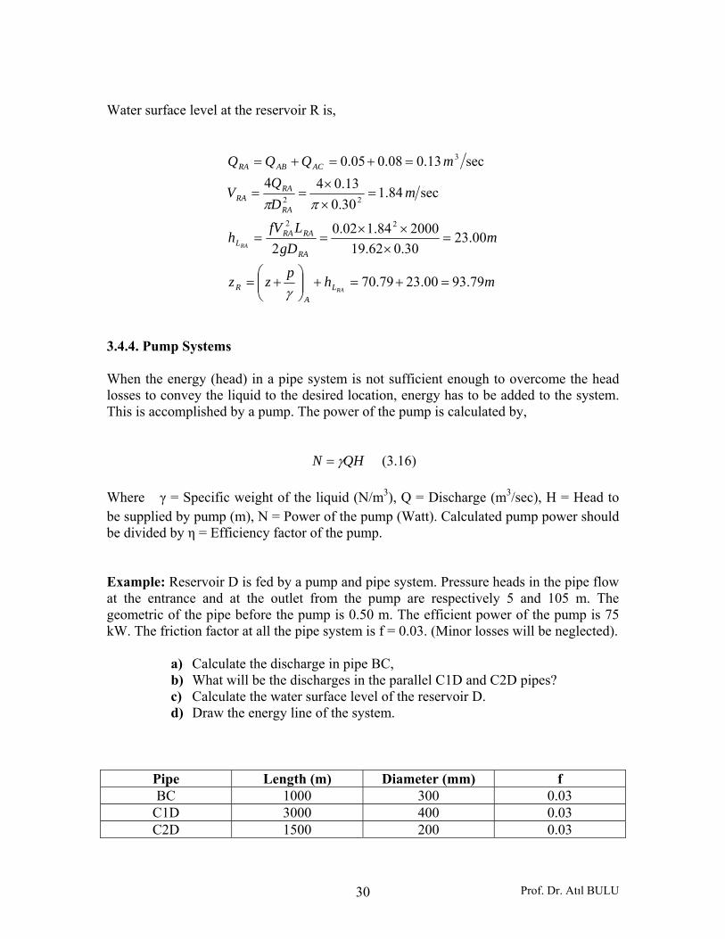
Where γ = Specific weight of the liquid (N/m3), Q = Discharge (m3/sec), H = Head to be supplied by pump (m), N = Power of the pump (Watt). Calculated pump power should be divided by η = Efficiency factor of the pump. Example: Reservoir D is fed by a pump and pipe system. Pressure heads in the pipe flow at the entrance and at the outlet from the pump are respectively 5 and 105 m. The geometric of the pipe before the pump is 0.50 m. The efficient power of the pump is 75 kW. The friction factor at all the pipe system is f = 0.03. (Minor losses will be neglected).
a) Calculate the discharge in pipe BC, b) What will be the discharges in the parallel C1D and C2D pipes? c) Calculate the water surface level of the reservoir D. d) Draw the energy line of the system.
Pipe Length (m) Diameter (mm) f BC 1000 300 0.03
C1D 3000 400 0.03 C2D 1500 200 0.03
Prof. Dr. Atıl BULU 31
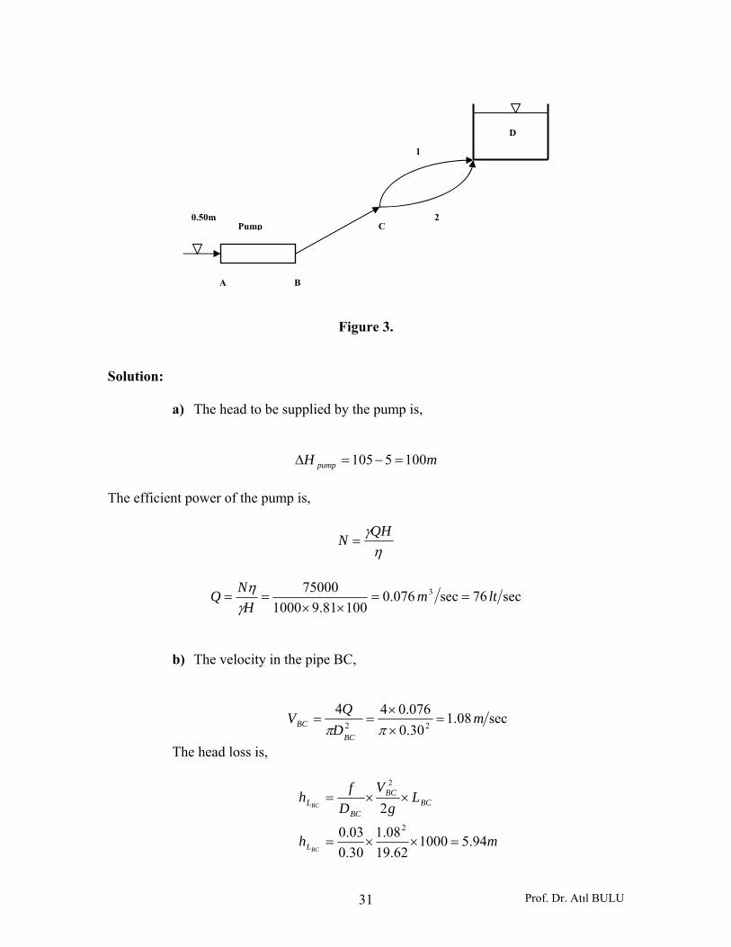
Figure 3.
Solution:
a) The head to be supplied by the pump is,
mH pump 1005105 =−=Δ
The efficient power of the pump is,
ηγQHN =
sec76sec076.010081.91000
75000 3 ltmH
NQ ==××
==γη
b) The velocity in the pipe BC,
sec08.130.0076.044
22 mD
QVBC
BC =××
==ππ
The head loss is,
mh
Lg
VD
fh
BC
BC
L
BCBC
BCL
94.5100062.19
08.130.003.0
22
2
=××=
××=
0.50m Pump
A B
C
1
2
D
Prof. Dr. Atıl BULU 32
Since,
VVVVV
gV
gV
Lg
VDfL
gV
Df
hh LL
===
××=××
××=××
=
21
22
21
22
21
2
22
21
21
1
1500220.0
03.03000240.0
03.0
22
21
By equation of continuity,
2
22
2
1
21
1
21
4
4
VD
Q
VD
Q
QQQ
×=
×=
+=
π
π
21
2
2
2
1
2
1
4440.0
42.0
416.0
44.0
VVQ
VVQ
=
×=××
=
×=××
=
ππ
ππ
sec765sec76
2
321
ltQmQQ
==+
sec2.151 ltQ = sec8.602 ltQ =
c) The velocity and the head loss in the parallel pipes are,
mLg
VDfhh
mVVV
LL 64.2300062.19
48.040.003.0
2
sec48.020.0
0152.04
2
1
2
1
221
21=××=××==
=××
===π
Prof. Dr. Atıl BULU 33
Total head loss is,
mh
hhh
L
LLL BC
58.864.294.51
=+=
+=
∑∑
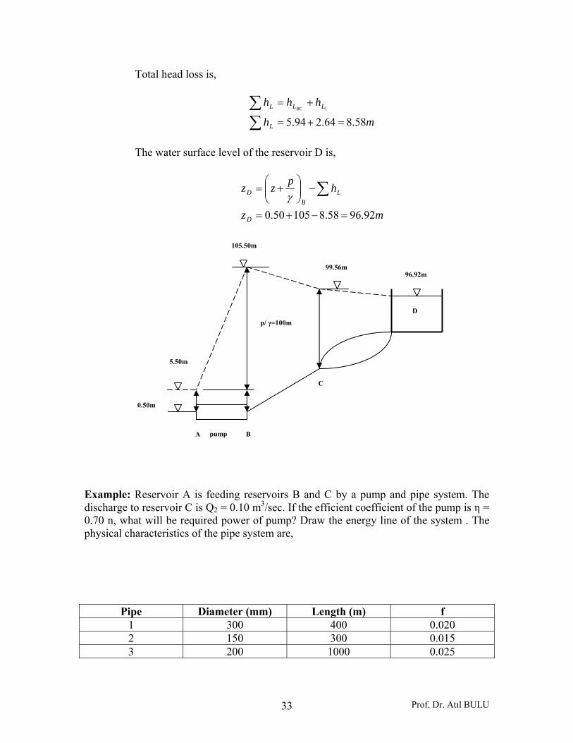
The water surface level of the reservoir D is,
mz
hpzz
D
LB
D
92.9658.810550.0 =−+=
−⎟⎟⎠
⎞⎜⎜⎝
⎛+= ∑γ
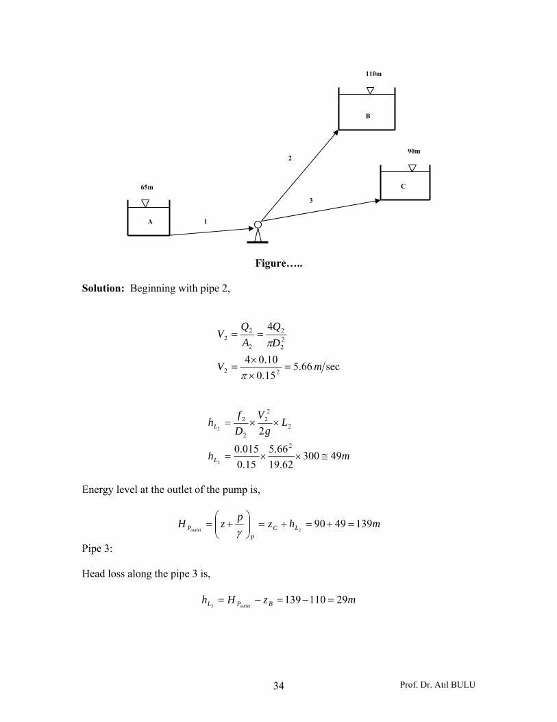
Example: Reservoir A is feeding reservoirs B and C by a pump and pipe system. The discharge to reservoir C is Q2 = 0.10 m3/sec. If the efficient coefficient of the pump is η = 0.70 n, what will be required power of pump? Draw the energy line of the system . The physical characteristics of the pipe system are,
Pipe Diameter (mm) Length (m) f 1 300 400 0.020 2 150 300 0.015 3 200 1000 0.025
5.50m
105.50m
99.56m96.92m
p/ γ=100m
A pump B
C
D
0.50m
Prof. Dr. Atıl BULU 34
Figure….. Solution: Beginning with pipe 2,
sec66.515.010.04
4
22
22
2
2
22
mV
DQ
AQ
V
=××
=
==
π
π
mh
Lg
VDf
h
L
L
4930062.19
66.515.0015.0
22
2
22
2
2
2
2
≅××=
××=
Energy level at the outlet of the pump is,
mhzpzH LCP
Poutlet1394990
2=+=+=⎟⎟
⎠
⎞⎜⎜⎝
⎛+=γ
Pipe 3: Head loss along the pipe 3 is,
mzHh BPL outlet29110139
3=−=−=
65m
A
B
C
110m
90m
1
2
3
Prof. Dr. Atıl BULU 35
sec067.013.24
20.04
sec13.2
100062.19200.0
025.029
2
32
3
23
3
3
23
3
23
3
33
mVD
Q
mV
V
Lg
VDf
hL
=××
=×=
=
××=
××=
ππ
Pipe 1:
mLg
VDf
h
mDQ
V
mQ
QQQ
L 57.740062.19
36.230.0
020.02
sec36.230.0167.044
sec167.0067.0100.0
2
1
21
1
1
221
11
31
321
1=××=××=
=××
==
=+=
+=
ππ
Energy level at the entrance to the pump is,
mhzH LAPent43.5757.700.65
1=−=−=
The energy (head) to be supplied by pump is,
mHHHentoutlet PPp 57.8143.5700.139 =−=−=Δ
The required power of the pump is,
kWWN
HQN
P
PP
19119095270.0
59.81167.0100081.9≅=
×××=
Δ=
ηγ
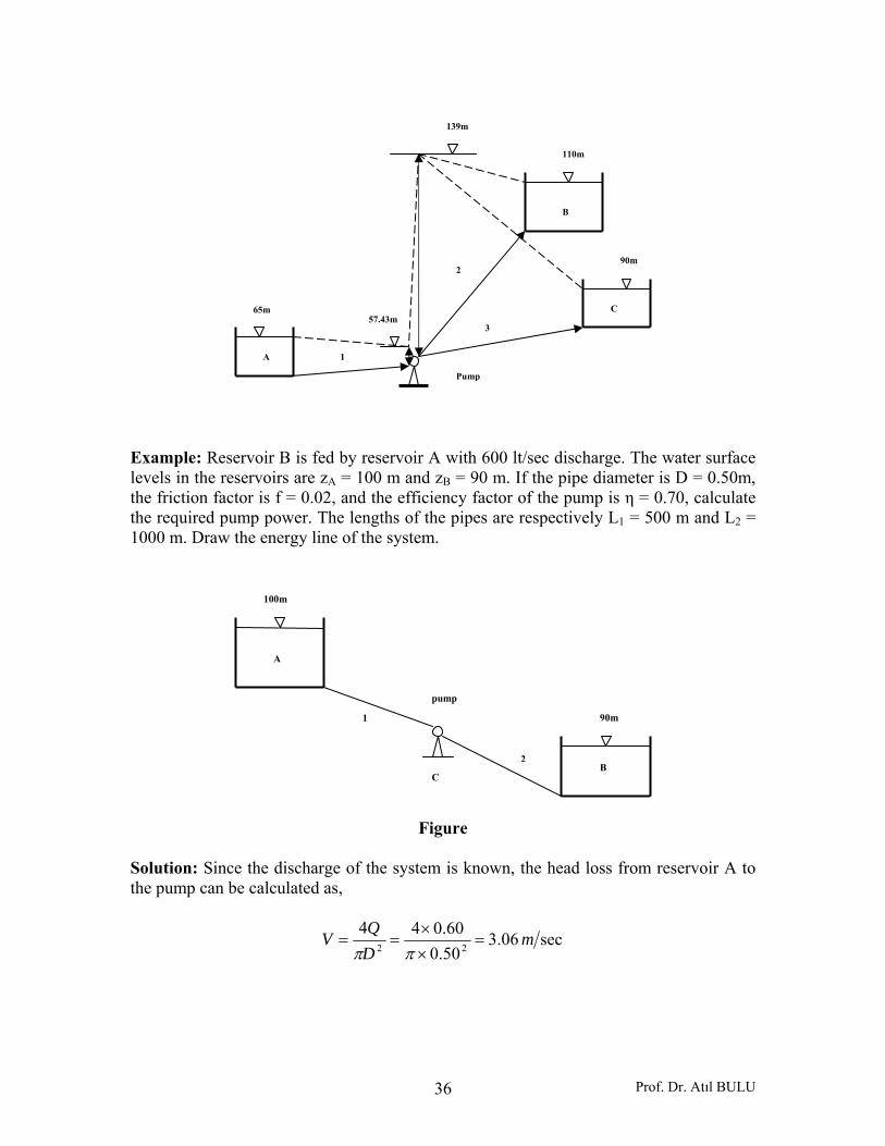
Prof. Dr. Atıl BULU 36
Example: Reservoir B is fed by reservoir A with 600 lt/sec discharge. The water surface levels in the reservoirs are zA = 100 m and zB = 90 m. If the pipe diameter is D = 0.50m, the friction factor is f = 0.02, and the efficiency factor of the pump is η = 0.70, calculate the required pump power. The lengths of the pipes are respectively L1 = 500 m and L2 = 1000 m. Draw the energy line of the system.
Figure Solution: Since the discharge of the system is known, the head loss from reservoir A to the pump can be calculated as,
sec06.350.060.044
22 mDQV =
××
==ππ
100m
90m
A
B C
pump
1
2
65m
A
B
C
110m
90m
1
2
3
139m
57.43m
Pump
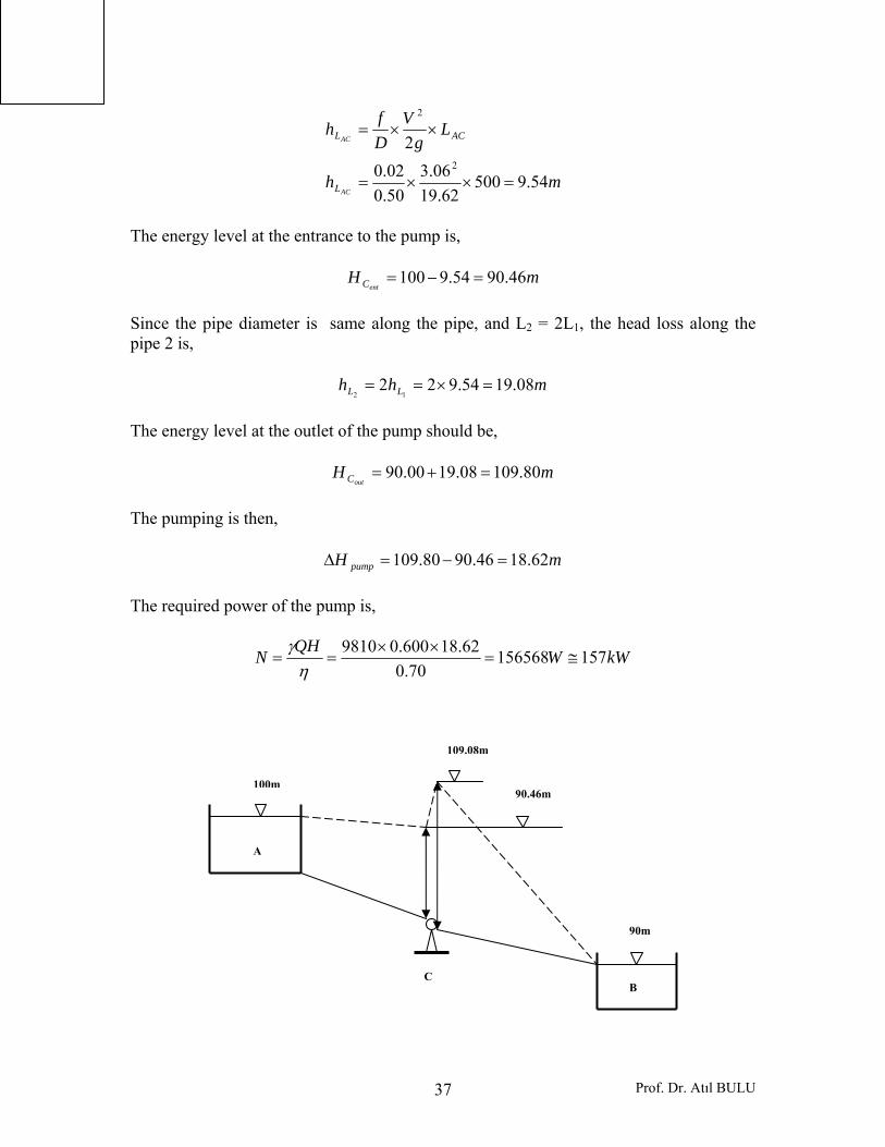
Prof. Dr. Atıl BULU 37
mh
Lg
VDfh
AC
AC
L
ACL
54.950062.19
06.350.002.0
22
2
=××=
××=
The energy level at the entrance to the pump is,
mHentC 46.9054.9100 =−=
Since the pipe diameter is same along the pipe, and L2 = 2L1, the head loss along the pipe 2 is,
mhh LL 08.1954.92212
=×==
The energy level at the outlet of the pump should be,
mHoutC 80.10908.1900.90 =+=
The pumping is then,
mH pump 62.1846.9080.109 =−=Δ
The required power of the pump is,
kWWQHN 15715656870.0
62.18600.09810≅=
××==
ηγ
A
100m
90m
C B
90.46m
109.08m