superior mathematics from an elementary point of view
TRANSCRIPT

HAL Id: cel-01813978https://cel.archives-ouvertes.fr/cel-01813978
Submitted on 12 Jun 2018
HAL is a multi-disciplinary open accessarchive for the deposit and dissemination of sci-entific research documents, whether they are pub-lished or not. The documents may come fromteaching and research institutions in France orabroad, or from public or private research centers.
L’archive ouverte pluridisciplinaire HAL, estdestinée au dépôt et à la diffusion de documentsscientifiques de niveau recherche, publiés ou non,émanant des établissements d’enseignement et derecherche français ou étrangers, des laboratoirespublics ou privés.
” Superior Mathematics from an Elementary point ofview ” course notes
Jacopo d’Aurizio
To cite this version:Jacopo d’Aurizio. ” Superior Mathematics from an Elementary point of view ” course notes. Master.Italy. 2017. �cel-01813978�

“Superior Mathematics from an Elementary point of view” course notesUndergraduate course, 2017-2018, University of Pisa
Jack D’Aurizio
Contents
0 Introduction 2
1 Creative Telescoping and DFT 3
2 Convolutions and ballot problems 15
3 Chebyshev and Legendre polynomials 30
4 The glory of Fourier, Laplace, Feynman and Frullani 40
5 The Basel problem 60
6 Special functions and special products 70
7 The Cauchy-Schwarz inequality and beyond 97
8 Remarkable results in Linear Algebra 121
9 The Fundamental Theorem of Algebra 125
10 Quantitative forms of the Weierstrass approximation Theorem 133
11 Elliptic integrals and the AGM 137
12 Dilworth, Erdos-Szekeres, Brouwer and Borsuk-Ulam’s Theorems 147
13 Continued fractions and elements of Diophantine Approximation 158
14 Symmetric functions and elements of Analytic Combinatorics 173
15 Spherical Trigonometry 183
0 Introduction
This course has been designed to serve University students of the first and second year of Mathematics. The purpose
of these notes is to give elements of both strategy and tactics in problem solving, by explaining ideas and techniques
willing to be elementary and powerful at the same time. We will not focus on a single subject among Calculus,
Algebra, Combinatorics or Geometry: we will just try to enlarge the “toolbox” of any professional mathematician
wannabe, by starting from humble requirements:
• knowledge of number sets (N,Z,Q,R,C) and their properties;
• knowledge of mathematical terminology and notation;
• knowledge of the main mathematical functions;
• knowledge of the following concepts: limits, convergence, derivatives, Riemann integral;

1 CREATIVE TELESCOPING AND DFT
• knowledge of basic Combinatorics and Arithmetics.
A collection of problems in Analysis and Advanced integration techniques, kindly provided by Tolaso J. Kos and Zaid
Alyafeai, are excellent sources of exercises to match with the study of these notes.
These notes are distributed under a Creative Commons Share-Alike (CCSA) license. Personal use is allowed,
distribution is allowed with the only contraint of making a proper mention of the author (Jack D’Aurizio).
Commercial use, modification or inclusion in other works are not allowed.
1 Creative Telescoping and DFT
It is soon evident, during the study of Mathematics, that the bijectivity of some function f does not grant that the
explicit computation of f−1(y) is “just as easy” as the explicit computation of f(x). Some examples are related
with the ease of multiplication, against the hardness of factorization; the possibility of computing derivatives in a
algorithmic fashion, against the lack of a completely algorithmic way to find indefinite integrals; the determination of
a Galois group of an irreducible polynomial over Q, against the difficult task of finding a polynomial having a given
Galois group. In the present section we will outline two interesting techniques for solving (or getting arbitrarily close
to an actual “solution”) a peculiar inverse problem, that is the computation of series.
Definition 1. We give the adjective telescopic to objects of the form a1 + a2 + . . .+ an, where each ai can be written
as bi − bi+1 for some sequence b1, b2, . . . , bn, bn+1. With such assumption we have:
a1 + a2 + . . .+ an = (b1 − b2) + (b2 − b3) + . . .+ (bn − bn+1) = b1 − bn+1.
Essentially, every telescopic sum is simple to compute, just as any convergent series with terms of the form bi − bi+1.
A peculiar example is provided by Mengoli series: the identity
N∑n=1
1
n(n+ 1)=
N∑n=1
(1
n− 1
n+ 1
)= 1− 1
N + 1
grants we have ∑n≥1
1
n(n+ 1)= 1.
The following generalization is also straightforward:
Lemma 2.
∀k ∈ N+,∑n≥1
1
n(n+ 1) · . . . · (n+ k)=
1
k · k!.
In a forthcoming section we will also see a proof not relying on telescoping, but on properties of Euler’s Beta function.
The first technical issue we meet in this framework is related to the fact that recognizing a contribution of the form
bi − bi+1 in the general term of a series is not always easy, just like in the continuous analogue: if the task is to
find∫ baf(x) dx, it is not always easy to devise a function g such that f(x) = g′(x). Here there are some non-trivial
examples:
Lemma 3. ∑n≥1
arctan
(1
1 + n+ n2
)=π
4.
Page 3 / 195

Proof. If we use “backwards” the sum/subtraction formulas for the tangent function, we have that
tan(x± y) =tan(x)± tan(y)
1∓ tan(x) tan(y)
implies:
arctan1
n− arctan
1
n+ 1= arctan
(1n −
1n+1
1 + 1n(n+1)
)= arctan
(1
1 + n+ n2
)so the given series is telescopic and it converges to arctan(1) = π
4 .
Exercise 4. The sequence of Fibonacci numbers {Fn}n≥0 is defined through F0 = 0, F1 = 1
and Fn+2 = Fn+1 + Fn for any n ≥ 0. Show that:
∑n≥1
arctan
((−1)n+1
Fn+1(Fn + Fn+2)
)= arctan(
√5− 2).
Exercise 5. Show that:∑n∈Z
arctan
(sinh 1
cosh(2n)
)=π
2,
∑n≥1
arctan
(1
8n2
)=π
4− arctan tanh
π
4.
Exercise 6. Prove that:N∑n=0
1
4n
(2n
n
)=N + 1
22N+1
(2N + 2
N + 1
),
for instance by considering that by De Moivre’s formula we have
An =1
4n
(2n
n
)=
1
2π
∫ π
−πcos2n(x) dx
since cos(x)2n = 14n
∑2nj=0
(2nj
)e(2n−j)ixe−jix and
∫ π−π e
kix dx = 2π · δ(k),
so the only non-vanishing contribution is related to the j = n term, and
N∑n=0
1
4n
(2n
n
)=
1
2π
∫ π
−π
1− cos2N+2(x)
sin2(x)dx = (2N + 2)AN+1 =
N + 1
22N+1
(2N + 2
N + 1
)follows from the integration by parts formula (
∫dx
sin2 x= − cotx). Prove also that
∑k≥0
(2k
k
)1
(k + 1)4k= 1
by recognizing in the main term a telescopic contribution. Give a probabilistic interpretation to the proved identities,
by considering random paths on a infinite grid (Z×Z) where only unit movements towards North or East are allowed.
We now outline the first (really) interesting idea, namely creative telescoping: even if we are not able to write the
main term of a series in the bi− bi+1 form, it is not unlikely there is an accurate approximation of the main term that
can be represented in such a telescopic form. By subtracting the accurate telescopic approximation from the main
term, the original problem boils down to computing/approximating a series that is likely to converge faster than the
Page 4 / 195

1 CREATIVE TELESCOPING AND DFT
original one, and the same approximation-by-telescopic-series trick can be performed again. For instance, we might
employ creative telescoping for producing very accurate approximations of the series
ζ(2) =∑n≥1
1
n2
that will be the main character of a forthcoming section.
In particular, for any n > 1 the term 1n2 is quite close to the telescopic term 1
n2− 14
:
1
n2 − 14
=4
(2n− 1)(2n+ 1)= 2
(1
2n− 1− 1
2n+ 1
)and we have 1
n2 − 1n2− 1
4
= − 1(2n−1)n2(2n+1) , so:
ζ(2) = 1 +∑n≥2
1
n2= 1 +
∑n≥2
1
n2 − 14
−∑n≥2
1
(2n− 1)n2(2n+ 1)
= 1 +2
3−∑n≥2
1
(2n− 1)n2(2n+ 1)
gives us ζ(2) < 53 (that we will prove to be equivalent to π2 < 10), and the magenta “residual series” can be manipu-
lated in the same fashion (by extracting the first term, approximating the main term with a telescopic contribution,
considering the residual series) or simply bounded above by:∑n≥2
1
(2n− 1)n2(2n+ 1)<∑n≥2
1
(2n− 1)(n− 1
2
) (n+ 1
2
)(2n+ 1)
=3
2ζ(2)− 22
9
from which the lower bound ζ(2) > 7445 follows. We may notice that the difference between 74
45 and 53 is already pretty
small. In this framework the iteration of creative telescoping leads to two interesting consequences: the identity
ζ(2) =∑n≥1
1
n2=∑n≥1
3
n2(
2nn
) ,
providing a remarkable acceleration of the series defining ζ(2), and Stirling’s inequality:
(ne
)n√2πn exp
(1
12n+ 1
)≤ n! ≤
(ne
)n√2πn exp
(1
12n
)
further details will be disclosed soon.
It is also possible to employ creative telescoping for proving that:
ζ(3) =∑n≥1
1
n3=
5
2
∑n≥1
(−1)n+1
n3(
2nn
)
a key identity in Apery’s proof of ζ(3) 6∈ Q.
We may notice that:1
n3=
1
(n− 1)n(n+ 1)+
(−1)
(n− 1)n3(n+ 1)
1
(n− 1)n3(n+ 1)=
1
(n− 2)(n− 1)n(n+ 1)(n+ 2)+
−22
(n− 2)(n− 1)n3(n+ 1)(n+ 2)
Page 5 / 195

Continuing on telescoping we get that:
1
n3=
(−1)mm!2
(n−m) . . . n3 . . . (n+m)+
m∑j=1
(−1)j−1(j − 1)!2
(n− j) . . . (n+ j)
So by setting m = n− 1:
1
n3=
(−1)n−1(n− 1)!2
n2(2n− 1)!+
n−1∑j=1
(−1)j−1(j − 1)!2
(n− j) . . . (n+ j)
The terms of the last series can be managed through partial fraction decomposition:
1
(n− j) . . . (n+ j)=
1
(2j)!(n− j)− 1
(2j − 1)!1!(n− j + 1)+
1
(2j − 2)!2!(n− j + 2)− . . .
(n− j − 1)!
(n+ j)!=
2j∑k=0
(−1)k
(2j − k) k! (n− j + k)=
1
(2j)!
2j∑k=0
(−1)k(
2jk
)n− j + k
and since: ∑n>j
2j∑k=0
(−1)k(
2jk
)n− j + k
=
2j∑h=1
(−1)h−1(
2j−1h−1
)h
=
∫ 1
0
(1− x)2j−1 dx =1
2j
we get:
ζ(3) =
+∞∑n=1
(−1)n−1n!2
n4(2n− 1)!+
+∞∑j=1
∑n>j
(−1)j−1(j − 1)!2
(n− j) . . . (n+ j)
ζ(3) =
+∞∑n=1
(−1)n−1n!2
n4(2n− 1)!+
+∞∑j=1
(−1)j−1j!2
2j3 (2j)!=
5
2
+∞∑n=1
(−1)n−1
n3(
2nn
)as wanted.
Exercise 7. Prove that the following identity (about the acceleration of an “almost-geometric” series) holds.∑n≥2
1
2n − 1=
1
4+∑m≥2
8m + 1
(2m − 1)2m2+m.
As proved by Tachiya, this kind of acceleration tricks provide a simple way for proving the irrationality
of∑n≥1
1qn+1 and
∑n≥1
1qn−1 for any q ∈ Z such that |q| ≥ 2.
Creative telescoping can also be used for a humble purpose, like proving the divergence of the harmonic series.
By recalling that the n-th harmonic number Hn is defined through
Hn =
n∑k=1
1
k
and by recalling that over the interval (0, 1] we have:
x < 2 arctanh(x
2
)= log
(1 + x
2
1− x2
)it follows that:
Hn <
n∑k=1
log
(2k + 1
2k − 1
)= log(2n+ 1).
On the other hand 2 arctanh(x2
)− x = O(x3) in a neighbourhood of the origin, and the series
∑k≥1
1k3 = ζ(3) is
convergent, so there is an absolute constant C granting Hn ≥ log(2n + 1) − C for any n ≥ 1. In a similar way, by
defining the n-th generalized harmonic number H(j)n through
H(j)n =
n∑k=1
1
kj,
Page 6 / 195

1 CREATIVE TELESCOPING AND DFT
we may easily check that the sequence {an}n≥1 defined by
an = 2√n−H(1/2)
n = 2√n−
n∑k=1
1√k
is increasing and never exceeds a constant close to 1 + 1√5. About an+1 ≥ an we have:
an+1 − an = 2√n+ 1− 2
√n− 1√
n+ 1=
112
(√n+√n+ 1
) − 1√n+ 1
=1
√n+ 1
(√n+√n+ 1
)2 > 0
and
an =
n∑m=0
1√m+ 1
(√m+
√m+ 1
)2 −→n→+∞
∑n≥0
1√n+ 1
(√n+√n+ 1
)2 .The claim then follows from considering that the main term of the last series is well-approximated by the telescopic
term1√
4n+ 1− 1√
4n+ 5
for any n ≥ 1. In similar contexts, by exploiting creative telescoping and the Cauchy-Schwarz inequality we may get
surprising results, like the following one:
n∑k=1
1
n+ k<
n∑k=1
1√n+ k − 1
√n+ k
CS≤
√√√√n
n∑k=1
(1
n+ k − 1− 1
n+ k
)=
1√2
but the limit of the LHS for n → +∞ is log(2), hence log(2) ≤ 1√2. In general, by mixing few ingredients among
creative telescoping, the Cauchy-Schwarz inequality, convexity arguments and Weierstrass products we may achieve
short and elegant proofs of highly non-trivial claims, like:
Lemma 8. The sequence {an}n≥1 defined through
an =
(2n
n
)√π (n+ 14
)4n
is increasing and convergent to 1, due to the identity
(2n+ 1)2(4n+ 5)− 4(n+ 1)2(4n+ 1) = 1.
That impliesΓ(x+ 1
2
)Γ(x)
∼ x√x+ 1/4
for any x > 0, that is a strengthening of Gautschi’s inequality.
Creative telescoping is also a key element in the Wilf and Zeilberger algorithm for the symbolic computation of binomial
sums (http://mathworld.wolfram.com/Wilf-ZeilbergerPair.html), further extended by Gosper to the hyperge-
ometric case and by Risch (https://en.wikipedia.org/wiki/Risch_algorithm) to the symbolic computation of
elementary antiderivatives.
Exercise 9. Prove by creative telescoping that for any k ∈ {2, 3, 4, . . .} we have:∑n≥1
1
n(n+ 1)k= k − ζ(2)− . . .− ζ(k)
where ζ(m) =∑n≥1
1nm .
Page 7 / 195

Before introducing a second tool (the discrete Fourier transform, DFT ), it might be interesting to consider an appli-
cation of creative telescoping to the computation of an integral.
Exercise 10. Prove that the following identity holds:∫ 1
0
log(x) log2(1− x)
xdx = −1
2
∑n≥1
1
n4= −ζ(4)
2.
Proof. The dilogarithm function is defined, for any x ∈ [0, 1], through:
Li2(x) =∑n≥1
xn
n2.
We may notice that Li′2(x) = − log(1−x)x , so, by integration by parts:∫ 1
0
log(x)Li2(x)
1− xdx =
∫ 1
0
log(1− x)
[Li2(x)
x+ log(x)Li′2(x)
]dx
= −∫ 1
0
Li′2(x)Li2(x) dx−∫ 1
0
log(x) log2(1− x)
xdx
In particular the opposite of our integral equals:
−∫ 1
0
log(x) log2(1− x)
xdx =
1
2Li22(1) +
∫ 1
0
∑n≥1
xn
n2
∑k≥0
xk log(x) dx
=1
2ζ(2)2 −
∑n≥1
1
n2
∑m>n
1
m2
where, by symmetry: ∑m>n≥1
1
m2n2=
1
2
∑n≥1
1
n2
2
−∑n≥1
1
n4
and the claim readily follows. We may notice that:
log2(1− x)
x=∑n≥0
2Hn
(n+ 1)xn,
since:
− log(1− x) =∑n≥1
xn
n
− log(1− x)
1− x=∑n≥1
Hn xn 1
2log2(1− x) =
∑n≥1
Hn
n+ 1xn+1
By termwise integration (through∫ 1
0(− log x)xn dx = 1
(n+1)2 ) the proved identities lead to:
∑n≥1
Hn
(n+ 1)3=
1
4
∑n≥1
1
n4=ζ(4)
4.
A keen reader might ask why this virtuosity has been included in the creative telescoping section. The reason is
the following: in order to make the magic work, we actually do not need the dilogarithm function (a mathematical
function with the sense of humour, according to D.Zagier) or integration by parts. As a matter of fact:
Hn =
n∑k=1
1
k=∑m≥1
(1
m− 1
m+ n
)=∑m≥1
n
m(m+ n)
Page 8 / 195

1 CREATIVE TELESCOPING AND DFT
hence it follows that:∑n≥1
Hn
(n+ 1)3=
∑n≥1
(Hn+1
(n+ 1)3− 1
(n+ 1)4
)= −ζ(4) +
∑n≥1
Hn
n3
= −ζ(4) +∑n,m≥1
1
mn2(m+ n)= −ζ(4) +
1
2
∑m,n≥1
(1
mn2(m+ n)+
1
m2n(m+ n)
)= −ζ(4) +
1
2
∑m,n≥1
1
m2n2= −ζ(4) +
1
2ζ(2)2
and by comparing the last identity to the identities we already know, we get that ζ(4) = 25ζ(2)2.
Some questions might naturally arise at this point: is it possible, in a similar fashion, to relate the value of ζ(2k+1)
to the value of ζ(2k)? Or: is it possible to find the explicit value of ζ(2) by simply squaring the Taylor series at the
origin of the arctangent function? Answers to such questions are postponed.
We directly introduce the DFT through a problem.
Exercise 11. Let A be a finite set with cardinality ≥ 4. Let P0 be the set of subsets of A with 3j elements, let P1 be
the set of subsets of A with 3k + 1 elements, let P2 be the set of subsets of A with 3h + 2 elements. Prove that any
two numbers among |P0|, |P1|, |P2| differ at most by 1, no matter what |A| is.
The claim appears to be a (more or less) direct generalization of a well-known fact: the number of subsets of I =
{1, 2, . . . , n} with even/odd cardinality is the same. In that framework, we may consider the map sending B ⊆ I in
B \ {1} when 1 ∈ B, and in B ∪ {1} when 1 6∈ B (“if there is 1, we remove it, otherwise we insert it”): such map is
an involution and provides a bijection between the subsets with even cardinality and the subsets with odd cardinality.
As an alternative, by recalling that in I we have(nk
)subsets with k elements, we may simply check that
n∑k=0
(n
k
)(−1)k = 0
holds as a trivial consequence of the binomial Theorem applied to (1− 1)n.
In the ternary case we have to compare the sums
|P0| =∑
k≡0 (mod 3)
(n
k
), |P1| =
∑k≡1 (mod 3)
(n
k
), |P2| =
∑k≡2 (mod 3)
(n
k
)
and we would like to have a tool allowing us to isolate the contributions given by elements in particular positions
(positions given by an arithmetic progression) in a sum. The DFT is precisely such a tool.
Lemma 12 (DFT). If n ≥ 2 is a natural number and ω = exp(
2πin
), the function f : Z→ C given by
f(m) =1
n
n−1∑k=0
ωkm
is the indicator function of nZ. As a consequence,
χh(m) =1
n
n−1∑k=0
ω−hkωkm
is the indicator function of the integers ≡ h(mod n).
Page 9 / 195

The possibility of writing some indicator functions as weigthed power sums has deep consequences.
In our case, if we take ω as a primitive third root of unity, we have:
|P0| =n∑k=0
(n
k
)χ0(k) =
1
3
n∑k=0
(n
k
)(1k + ωk + ω2k
)=
(1 + 1)n + (1 + ω)n + (1 + ω2)n
3
due to the binomial Theorem. Since both (1 + ω) and its conjugate (1 + ω2) lie on the unit circle, we have that |P0|is an integer number whose distance from 2n
3 is bounded by 13 . The reader can easily check the same holds for |P1|
and |P2| and the claim readily follows. The discrete Fourier transform proves so the reasonable proposition claiming
the almost-uniform distribution of the cardinality (mod 3) of subsets of {1, . . . , n}. Perfect uniformity is clearly not
possible, since |P0|+ |P1|+ |P2| = 2n never belongs to 3Z.
Exercise left to the reader: prove the claim of Exercise 11 by induction on |A|.
Exercise 13. Find the explicit value of the series:
S =∑n≥0
1
(3n)!.
We may consider that the complex exponential function
ez =∑n≥0
zn
n!
is defined by an everywhere-convergent power series, then apply a ternary DFT to such series and get, like in the
previous exercise (here we are manipulating an infinite sum, but there is no issue since ez is an entire function):
∑n≥0
z3n
(3n)!=
∑n≡0 (mod 3)
zn
n!=∑n≥0
zn
n!χ0(n) =
1
3
∑n≥0
zn + (ωz)n + (ω2z)n
n!=
1
3
(ez + eωz + eω
2z)
and since ω = −1+i√
32 and ω2 = −1−i
√3
2 , for any z ∈ C we have:
∑n≥0
z3n
(3n)!=
1
3
(ez + 2e−z/2 cos
z√
3
2
),
that by an evaluation at z = 1 leads to:
S =e
3+
2
3√e
cos
√3
2.
Was the introduction of the complex z variable really necessary? It clearly was not: a viable alternative would have
been to just re-write 1 as 1n in the definition of S. Besides the identity 1 = 1n being really obvious, the idea of tackling
the original problem through such identity and the DFT is not obvious at all: similar situations explain just fine the
subtle difference between the adjectives elementary and easy in a mathematical context. Another famous application
of the DFT is related with the Frobenius coin problem:
Exercise 14. Given n ∈ N, let Un be the number of natural solutions of the (diophantine) equation a+ 2b+ 3c = n,
i.e.
Un =∣∣{(a, b, c) ∈ N3 : a+ 2b+ 3c = n
}∣∣ .Prove that for any n, Un equals the closest integer to (n+3)2
12 .
Page 10 / 195

1 CREATIVE TELESCOPING AND DFT
This claim will be proved in the section about Analytic Combinatorics, since few elements of Complex Analysis and
manipulation of formal power series are required. However we remark that the key idea is the same key idea of
Hardy-Littlewood’s circle method, a really important tool in Additive Number Theory: for instance, it has been used
for proving that any odd natural number large enough is the sum of three primes (Chen’s theorem, also known as
ternary Goldbach). Now we will focus on a typical application of the DFT in Arithmetics, i.e. a proof of a particular
case of Dirichlet’s Theorem.
Theorem 15 (Dirichlet). If a and b are coprime positive integers, there are infinite prime numbers ≡ a (mod b).
The particular case we are going to study is the proof of the existence of infinite primes of the form 6k+ 1. We recall
that the infinitude of primes of the form 6k − 1 follows from a minor variation on Euclid’s proof of the infinitude of
primes:
Let us assume the set of primes of the form 6k − 1 is finite and given by {p1 = 5, 11, 17, . . . , pM} = E.
Let us consider the huge number
N = −1 + 6
M∏m=1
pm.
By construction, no element of E divides N . On the other hand, N is a number of the form 6K − 1, hence it
must have some prime divisor ≡ −1 (mod 6). Such contradiction leads to the fact that the set of primes of the
form 6k − 1 is not finite (aka infinite).
We may notice that a number of the form 6k + 1 is not compelled to have a prime divisor of the same form (for
instance, 55 = 5 · 11), so the previous argument is not well-suited for covering the 6k + 1 case, too. 1 We then take a
step back and a step forward: we provide an alternative proof of the infinitude of primes, then prove it can be adjusted
to prove the existence of infinite primes of the form 6k+ 1, too. Let us recall the main statement in Analytic Number
Theory:
Theorem 16 (Euler’s product for the ζ function). If P is the set of prime numbers and s is a complex number with
real part greater than one, ∏p∈P
(1− 1
ps
)−1
=∑n≥1
1
ns= ζ(s).
Since(
1− 1ps
)−1
= 1 + 1ps + 1
p2s + . . ., such result is just the analytic counterpart of the Fundamental Theorem of
Arithmetics, stating that Z is a UFD.
In such framework the following argument is pretty efficient: if there were just a finite number of primes, given Euler’s
product the harmonic series would be convergent. But we know it is not, so there have to be an infinite number of
primes. The Theorem just outlined has an interesting generalization:
Theorem 17 (Euler’s product for Dirichlet’s L-functions). If P is the set of prime numbers, s is a complex number with
real part greater than one and χ(n) is a totally multiplicative function (i.e. a function such that χ(nm) = χ(n)χ(m)
holds for any couple (n,m) of positive integers), we have:∏p∈P
(1− χ(p)
ps
)−1
=∑n≥1
χ(n)
ns= L(s, χ).
1However, there is a light that never goes out: the infinitude of primes of the form 6k + 1 can be proved in a algebraic fashion by
considering cyclotomic polynomials. For instance, every prime divisor of Φ6(3n) = 9n2 − 3n+ 1 is a number of the form 6k + 1.
Page 11 / 195

We may consider a simple totally multiplicative function: the function that equals 1 over natural numbers ≡ 1(mod 6),
−1 over natural numbers ≡ −1(mod 6) and zero otherwise. Such function is the non-principal (Dirichlet) character
(mod 6). We may notice that: ∑n≥1
zn
n= − log(1− z)
for any complex number z having modulus less than one. By applying the DFT with respect to a primitive sixth root
of unity:
L(1, χ) =∑k≥0
(1
6k + 1− 1
6k + 5
)=
π
2√
3.
As an alternative:
L(1, χ) =∑k≥0
(1
6k + 1− 1
6k + 5
)=∑k≥0
∫ 1
0
(x6k − x6k+4) dx
=
∫ 1
0
(1− x4)∑k≥0
x6k dx =
∫ 1
0
1− x4
1− x6dx
=
∫ 1
0
1 + x2
1 + x2 + x4dx =
π
2√
3
Let us assume that prime numbers ≡ 1 (mod 6) are finite and consider Euler’s product for L(s, χ):
L(s, χ) =∏
p≡1 (mod 6)
(1− 1
ps
)−1 ∏p≡−1 (mod 6)
(1 +
1
ps
)−1
≤∏
p≡1 (mod 6)
(1− 1
p
)−1 ∏p≡−1 (mod 6)
(1 +
1
ps
)−1
= C∏p 6=2,3
(1 +
1
ps
)−1
= D∏p
(1 +
1
ps
)−1
= Dζ(2s)
ζ(s)
for some constant D > 0. From the divergence of the harmonic series we would have:
lims→1+
L(s, χ) = 0,
but we already know that L(1, χ) > 0 (we computed its explicit value).
Such contradiction leads to the fact that the set of primes of the form 6k + 1 is infinite.
We underline some points in the proof just outlined:
• we used Euler’s product, analytic counterpart of the Fundamental Theorem of Arithmetics, for studying the
distribution of primes in the arithmetic progressions (mod 6). It looks highly unlikely that there is just a finite
number of primes ≡ 1(mod 6) and infinite primes ≡ −1(mod 6), so we just need to show that such awkward
“imbalance” does not really occur;
• through the DFT, we may compute the value of L(1, χ) (with χ being the non-principal character (mod 6)) in
a explicit way, and check it is a positive number;
• from Euler’s product we have that the previous “imbalance” would lead to L(1, χ) = 0. It is not so, hence there
is no “imbalance”.
Page 12 / 195

1 CREATIVE TELESCOPING AND DFT
At last, we mention that both the DFT and the existence of Dirichlet’s characters are instances of Pontryagin’s duality
(https://en.wikipedia.org/wiki/Pontryagin_duality). The DFT is also of great importance for algorithms, since
it gives methods for the fast multiplication of polynomials (or integers): in such a context it is also known as FFT
(Fast Fourier Transform). Summarizing:
• The key idea is to exploit interpolation/extrapolation. A polynomial with degree m is fixed by its values at
m+ 1 distinct points. If we assume to have a(x) and b(x) and we need to compute c(x) = a(x) · b(x), we may. . .
• compute in a explicit way the values of a and b at the 2n-th roots of unity, then the values of c at such points. . .
• and compute the coefficients of c(x) through such values. Nicely, both the evaluation process and the extrapola-
tion process are associated with a matrix-vector-product problem, where the involved matrix is Vandermonde’s
matrix given by the 2n-th roots of unity;
• the structure of such matrix depends in a simple way from the structure of Vandermonde’s matrix given by the
2n−1-th roots of unity, hence the needed matrix-vector-products can be computed through a recursive, divide et
impera approach, with a significant improvement in computational costs.
For further details, please see http://en.wikipedia.org/wiki/Cooley-Tukey_FFT_algorithm.
The formulas of Koecher, Leshchiner and Bailey-Borwein-Bradley.
We have studied how to use the creative telecoping machinery for producing fast-convergent series representing
ζ(2) or ζ(3). Three formulas provide a wide generalization of such statement. The first one is due to Koecher
(1979): ∑n≥0
ζ(2n+ 3)a2n =∑k≥1
1
k(k2 − a2)=
1
2
∑k≥1
(−1)k+1
k3(
2kk
) · 5k2 − a2
k2 − a2
k−1∏m=1
(1− a2
m2
),
the second one is due to Leschiner (1981):
∑n≥0
(1− 1
22n+1
)ζ(2n+ 2)a2n =
∑n≥1
(−1)n+1
n2 − a2=
1
2
∑k≥1
1
k2(
2kk
) · 3k2 + a2
k2 − a2
k−1∏m=1
(1− a2
m2
),
the third one is due to Bailey-Borwein-Bradley (2006):
∑n≥0
ζ(2n+ 2)a2n =∑k≥1
1
k2 − a2= 3
∑k≥1
1(2kk
)(k2 − a2)
k−1∏m=1
m2 − 4a2
m2 − a2.
They hold for any a ∈ (−1, 1): by comparing the coefficients of ah in the LHS/RHS one gets that ζ(m), for
any m ≥ 2, can be represented as a fast-convergent series involving central binomial coefficients and generalized
harmonic numbers. It is straightforward to recover the well-known results
ζ(2) = 3∑n≥1
1
n2(
2nn
) , ζ(3) =5
2
∑n≥1
(−1)n+1
n3(
2nn
)together with the lesser known results
ζ(4) =36
17
∑k≥1
1
k4(
2kk
) , G =∑k≥0
(−1)k
(2k + 1)2=
1
2
∑n≥0
2n
(2n+ 1)(
2nn
) n∑k=0
1
2k + 1.
The last identity can also be proved by computing integrals involving the arcsin2(x) function or by computing the
binomial transform of 1(2k+1)2 .
Page 13 / 195

Exercise 18. Prove the following identity:∑n≥2
arctanh
(1
n3
)=
log(3)− log(2)
2,
trivially leading to ζ(3) < 1 + 12 log 3
2 .
Exercise 19. By exploiting Euler’s product prove that
∀s > 1,∑m,n≥1
1
lcm(m,n)s=ζ(s)3
ζ(2s).
Proof. For any M ∈ N+ of the form M = pα11 · · · p
αkk , the number of solutions of lcm(n,m) = M
is given by (2α1 + 1) · · · (2αk + 1). It follows that the given series equals∑M≥1
1
Ms
∏p|M
(2νp(M) + 1)
and since M 7→∏p|M (2νp(M) + 1) clearly is a multiplicative function, by Euler’s product
∑m,n≥1
1
lcm(m,n)s=∏p∈P
(1 +
3
ps+
5
p2s+
7
p3s+ . . .
)=∏p∈P
ps(ps + 1)
(ps − 1)2=∏p∈P
1− 1p2s(
1− 1ps
)3 =ζ(s)3
ζ(2s).
Exercise 20. Prove the following identity:∫ 1
−1
log2(1− x)√1− x2
= π∑n≥1
(2nn
)H2n−1
n4n=π3
3+ π log2(2).
Exercise 21. The analytic continuation for the Riemann ζ function to the region Re(s) > 0 gives us the identity
ζ(
12
)= −2 +
∑k≥1
1√k(√k +√k + 1)2
.
Use creative telescoping to show that:
ζ(
12
)= −3
2+
1
2
∑k≥1
1√k√k + 1(
√k +√k + 1)3
= −35
24− 7
96
∑k≥1
1
k√k(k + 1)
√k + 1(
√k +√k + 1)3
+1
96
∑k≥1
1
k√k(k + 1)
√k + 1(
√k +√k + 1)7
.
Page 14 / 195

2 CONVOLUTIONS AND BALLOT PROBLEMS
2 Convolutions and ballot problems
We start this section by recalling a well-known identity:
Lemma 22.n∑k=0
(n
k
)2
=
(2n
n
).
Proof. The first proof we provide is based on a double counting argument. Let us assume to have a parliament
with n politicians in the left wing and n politicians in the right wing, and to be asked to count how many committees
with n politicians we may have. It is pretty clear such number is given by(
2nn
), i.e. the number of subsets with n
elements in a set with 2n elements. On the other hand, we may count such committees according to the number of
politicians from the left wing (k ∈ [0, n]) in them. There are(nk
)ways for choosing k politicians of the left wing from
the n politicians we have. If in a committee there are k politicians from the left wing, there are n− k politicians from
the right wing, and we have(n
n−k)
=(nk
)for selecting them. It follows that:(2n
n
)=
n∑k=0
(n
k
)(n
n− k
)=
n∑k=0
(n
k
)2
as wanted. The second proof is based on the fact that
(f ∗ g)(n)def=
n∑k=0
f(k) · g(n− k)
is the convolution between f and g.
Since(nk
)is the coefficient of xk in the Taylor series of (1 + x)n at the origin2,
(1 + x)n =
n∑k=0
(n
k
)xk =⇒ [xk](1 + x)n =
(n
k
)implies that:
n∑k=0
(n
k
)(n
n− k
)=
n∑k=0
[xk](1 + x)n · [xn−k](1 + x)n = [xn] [(1 + x)n · (1 + x)n] = [xn](1 + x)2n =
(2n
n
).
The second approach leads to a nice generalization of the first identity in the current section:
Theorem 23 (Vandermonde’s identity). ∑j+k=n
(a
j
)(b
k
)=
(a+ b
n
).
In the introduced convolution context the last identity simply follows from the trivial (1 + x)a · (1 + x)b = (1 + x)a+b.
We may notice that ∑n≥0
c(n)xn
·∑n≥0
d(n)xn
=∑n≥0
(c ∗ d)(n)xn
2The notation [xk] f(x) stands for the coefficient of xk in the Taylor/Laurent series of f(x) at the origin.
Page 15 / 195
is the Cauchy product between two power series. The interplay between analytic and combinatorial arguments
allows us to prove interesting things. For instance we may consider the function f(x) =√
1− x = (1− x)1/2, analytic
in a neighbourhood of the origin. It is not difficult to compute its Taylor series by the extended binomial theorem.
Moreover f(x)2 = (1−x) has a trivial Taylor series, hence by defining a(n) as the coefficient of xn in the Taylor series
of f(x), (a ∗ a)(n) always takes values in {−1, 0, 1}.
(1− x)1/2 =∑n≥0
(1/2
n
)(−1)nxn =
∑n≥0
(−1)n12 ·(
12 − 1
)· . . . ·
(12 − n+ 1
)n!
xn
=∑n≥0
(−1)n1 · (1− 2) · . . . (1− 2n+ 2)
2nn!xn
= 1−∑n≥1
(2n− 1)!!
(2n− 1) · (2n)!!xn = 1−
∑n≥1
(2n)!
(2n− 1) · (2n)!!2xn
= 1−∑n≥1
(2n
n
)xn
4n(2n− 1)
By differentiating with respect to x,1√
1− x=∑n≥0
(2n
n
)xn
4n
follows, and since 11−x = 1 + x+ x2 + x3 + . . ., if we set a(n) = 1
4n
(2nn
)we have (a ∗ a)(n) = 1, i.e.:
Lemma 24.n∑k=0
(2k
k
)(2n− 2k
n− k
)= 4n.
We may also notice that
1
1− x∑n≥0
a(n)xn =∑n≥0
(a ∗ 1)(n)xn =∑n≥0
(n∑k=0
a(k)
)xn
where the LHS equals
1
(1− x)√
1− x= 2
d
dx
(1√
1− x
)= 2
∑n≥1
(2n
n
)nxn−1
4n=∑n≥0
(2n+ 2
n+ 1
)2n+ 2
4n+1xn.
By comparing the last two RHSs we have an alternative proof of an identity claimed by Exercise 6:
N∑n=0
(2n
n
)1
4n=
(2N + 2
N + 1
)N + 1
22N+1.
Exercise 25 (Stars and bars). Prove that for any k ∈ N we have:
1
(1− x)k+1=∑n≥0
(n+ k
k
)xn.
Proof. We may tackle this question both in a combinatorial and in an analytic way. The coefficient of xn in the
product of (k+ 1) terms of the form (1 +x+x2 + . . .) is given by the number of ways for writing n as the sum of k+ 1
natural numbers. By stars and bars we know the number of ways for writing n as the sum of k + 1 positive natural
numbers is(n−1k
)and it is not difficult to finish from there. As an alternative, we may proceed by induction on k.
The claim is trivial in the k = 0 case, and since
1
(1− x)k+2=
1
1− x· 1
(1− x)k+1=∑n≥0
[(n+ k
k
)∗ 1
]xn
Page 16 / 195

2 CONVOLUTIONS AND BALLOT PROBLEMS
the inductive step follows from the hockey stick identity
n∑j=0
(k + j
k
)=
(n+ k + 1
k + 1
).
Exercise 26. Given the sequences of Fibonacci and Lucas numbers {Fn}n≥0 and {Ln}n≥0,
prove the following convolution identity:n∑k=0
FkFn−k =nLn − Fn
5.
Proof. Since Fibonacci numbers fulfill the relation Fn+2 = Fn+1 + Fn, by defining their generating function as
f(x) =∑n≥0
Fnxn
we have that (1− x− x2) · f(x) is a linear polynomial (a similar idea leads to the Berkekamp-Massey algorithm).
On the other hand, if
f(x) =∑n≥0
Fnxn =
ax+ b
1− x− x2
b = 0 has to hold to grant f(0) = F0 = 0 and a = 1 has to hold to grant f ′(0) = F1 = 1. It follows that:
f(x) =x
1− x− x2=
1√5
(1
1− ϕx− 1
1− ϕx
), ϕ =
1 +√
5
2, ϕ =
1−√
5
2
and by computing the Taylor series (that is a geometric series) of 11−ϕx and 1
1−ϕx we immediately recover
Binet’s formula
Fn =ϕn − ϕn√
5.
The identity Ln = ϕn + ϕn has a similar proof. By starting the convolution machinery:
n∑k=0
FkFn−k = [xn]
(x
1− x− x2
)2
=1
5[xn]
(1
(1− ϕx)2+
1
(1− ϕx)2− 2
(1− ϕx)(1− ϕx)
)and the claim follows from simple fraction decomposition. To find a combinatorial proof is an exercise left to the
reader: we recall that Fibonacci numbers are related with subsets of {1, 2, . . . , n} without consecutive elements.
A note in mathematical folklore: Alon’s Combinatorial Nullstellensatz has further tightened the interplay
between combinatorial arguments and generating functions arguments. We invite the reader to delve into the
bibliography to find a generalization of Cauchy-Davenport’s theorem, once known as Kneser’s conjecture, now
known as Da Silva-Hamidoune’s Theorem:
Theorem 27 (Da Silva, Hamidoune). If A ⊆ Fp and A⊕A def= {a+ a′ : a, a′ ∈ A, a 6= a′}, we have:
|A⊕A| ≥ min(p, 2|A| − 3).
The convolution machinery applies very well to another kind of coefficients given by Catalan numbers. We introduce
them in a combinatorial fashion, assuming to have two people involved in a ballot and to check the votes one by one.
Page 17 / 195

Theorem 28 (Bertrand’s ballot problem). If the winning candidate gets A votes and the loser gets B votes (so we are
clearly assuming A > B), the probability that the winning candidate had the lead during the whole scrutiny equals:
A−BA+B
Proof. The final outcome is so simple due to a slick symmetry argument, applied in a double counting framework:
instead of trying to understand what happens or might happen once a single vote is checked, it is more effective to
consider which orderings of the votes favour A or not. Let us consider just the first vote: if it is a vote for B, at some
point of the scrutiny there must be a tie, since the winning candidate is A. If the first vote is for A and at some point
of the scutiny there is a tie, by switching the votes for A and for B till the tie we return in the previous situation. It is
pretty clear that the probability the first vote is a vote for B is BA+B . It follows that the probability of a tie happening
during the scrutiny is 2BA+B , and the probability that A always leads is:
1− 2B
A+B=A−BA+B
.
Theorem 29 (Catalan numbers). The number of strings made by n characters 0 and n characters 1,
with the further property that no initial substring has more 1s than 0s, is:
Cn =1
n+ 1
(2n
n
).
Proof. Any string with the given property can be associated (in a bijective way) with a path on a n×n grid, starting in
the bottom left corner and ending in the upper right corner, made by unit steps towards East (for each 1 character) or
North (for each 0 character) and never crossing the SW-NE diagonal (this translates the substrings constraint). These
paths can be associated in a bijective way with ballots that end in a tie, in which at every moment of the scrutiny the
votes for B are ≤ than the votes for A. If a deus ex machina adds an extra vote for A before the scrutiny begins, we
have a situation in which A gets n+ 1 votes, B gets n votes and A is always ahead of B. There are(
2n+1n
)=(
2n+1n+1
)possible scrutinies in which A gets n+ 1 votes and B gets n votes: by the previous result (Bertrand’s ballot problem)
the number of the wanted strings is given by:
(n+ 1)− n(n+ 1) + n
(2n+ 1
n
)=
1
2n+ 1
(2n+ 1
n
)=
1
n+ 1
(2n
n
).
For a slightly different perspective on the same subject, the reader is invited to have a look at Josef Rukavicka’s
“third proof” on the Wikipedia page about Catalan numbers.
Theorem 30. Given two natural numbers a and b with a ≥ b, the following identity holds:
b∑k=0
1
k + 1
(2k
k
)a− b
a+ b− 2k
(a+ b− 2k
b− k
)=
1 + a− b1 + a+ b
(a+ b+ 1
b
).
Proof. It is enough to count scrutinies for a ballot between two candidates A and B, with A getting a votes, B getting
b votes and A being always ahead of B, without excluding the chance of a tie at some point. We get the RHS by
adding an extra vote for A before the scrutiny begins and mimicking the previous proof. On the other hand we may
Page 18 / 195

2 CONVOLUTIONS AND BALLOT PROBLEMS
count such scrutinies according to the last moment in which we have a tie. If the last tie happens when 2k votes have
been checked, we simply need to assign a− k votes for A and b− k votes for B: what happens before the tie can be
accounted through Catalan numbers and what happens next through Bertrand’s ballot problem. This leads to the
LHS.
The last identity is a particular case of a remarkable generalization of Vandermonde’s identity(m+nr
)=∑rk=0
(mk
)(nr−k):
Theorem 31 (Rothe-Hagen).
n∑k=0
x
x+ kz
(x+ kz
k
)y
y + (n− k)z
(y + (n− k)z
(n− k)
)=
x+ y
x+ y + nz
(x+ y + nz
n
).
Proof. This identity is usually proved through generating functions and that approach is not terribly difficult. We may
point that a purely combinatorial proof is also possible, by following the lines of the previous proof. It is enough to
slightly modify the constraint at any point, the votes for B are ≤ than the votes for A by replacing it with something
involving the ratio of such votes. This is surprising both for experts and for newbies: Micheal Spivey has written an
interesting lecture about it on his blog.
The following problems are equivalent:
Exercise 32 (Balanced parenthesis). How many strings with 2n characters over the alphabet Σ = {(, )} have as
many open parenthesis as closed parenthesis, and in every initial substring the number of closed parenthesis is
always ≤ the number of open parenthesis?
Exercise 33 (Sub-diagonal paths). Let us consider the paths from (0; 0) to (n;n) where each step is a unit step
towards East or North. How many such paths belong to the region y ≤ x?
Exercise 34 (Triangulations of a polygon). Given a convex polygon, a triangulation of such polygon is a
partition in almost-disjoint triangles, with the property that every triangle has its vertices on the boundary of the
original polygon. How many triangulations are there for a convex polygon with n+ 2 sides?
Exercise 35 (Complete binary trees). A tree is a connected, undirected and acyclic graph. It is said binary
and complete if each vertex has two neighbours (in such a case it is an inner node) or no neighbours (in such a
case it is a leaf). How many complete binary trees with n inner nodes are there?
It is not difficult to prove the above claiming by exhibiting three combinatorial bijections:
TP←→ CBT←→ BP←→ SDP.
In each case the answer is given by the Catalan number
Cn =1
n+ 1
(2n
n
)where the sub-diagonal paths interpretation proves the identity
Cn+1 =
n∑k=0
CkCn−k
in a very straightfoward way. Such identity is a convolution formula: if we set c(x) =∑n≥0 Cnx
n,
we have c(x) = 1 + x · c(x)2. By solving such quadratic equation in c(x) we get:
c(x) =1−√
1− 4x
2x
Page 19 / 195

(the square root sign is chosen in such a way that c(x) is continuous at the origin) hence the coefficients of the
power series c(x) can be computed from the extended binomial theorem, extended since it is applied to (1− x)α with
α = 12 6∈ N.
Exercise 36. Prove that:
n∑k=0
(2n− 2k
n− k
)(2k
k
)1
2k + 1=
16n
(2n+ 1)(
2nn
) = 4n∫ π/2
0
cos(x)2n+1 dx.
The last identity is not trivial at all, and it has very deep consequences. A possible proof of such identity (that is
not the most elementary one: to find an elementary proof is an exercise we leave to the reader) exploits a particular
class of orthogonal polynomials. We have not introduced the L2 space yet, nor the usual techniques for dealing with
square-integrable objects, so such “advanced” proof is postponed to the end of this section, in a dedicated box. What
we can say through the convolution machinery is that the above identity is related with a Taylor coefficient in the
product between arcsin(x) and its derivative 1√1−x2
. By termwise integration it implies:
arcsin2(x) =1
2
∑n≥1
(4x2)n
n2(
2nn
)
and by evaluating the last identity at x = 12 we get that:
∑n≥1
3
n2(
2nn
) = 6 arcsin2
(1
2
)=π2
6
where the LHS equals ζ(2) by creative telescoping, as seen in the previous section, where we proved ζ(4) = 25ζ(2)2
too. It follows that:
ζ(2) =∑n≥1
1
n2=π2
6, ζ(4) =
∑n≥1
1
n4=π4
90.
We have just solved Basel problem through a very creative approach, i.e. by combining creative telescoping with
convolution identities for Catalan-ish numbers. Plenty of other approaches are presented in a forthcoming section.
Theorem 37 (Euler’s acceleration technique).
∑n≥0
(−1)nan =∑n≥0
(−1)n∆na0
2n+1, ∆na0 =
n∑k=0
(−1)k(n
k
)an−k.
This identity is simple to prove and it is really important in series manipulation and numerical computation: for
instance, it is the core of Van Wijngaarden’s algorithm for the numerical evaluating of series with alternating signs.
Let us study a consequence of Euler’s acceleration technique, applied to:
∑n≥0
(−1)n
2n+ 1=∑n≥0
∫ 1
0
(−1)nx2n dx =
∫ 1
0
dx
1 + x2= arctan(1) =
π
4
Page 20 / 195

2 CONVOLUTIONS AND BALLOT PROBLEMS
We may compute ∆na0 in a explicit way:
∆na0 =
n∑k=0
(−1)n−k(n
k
)1
2k + 1= (−1)n
∫ 1
0
n∑k=0
(n
k
)(−x2)k dx
= (−1)n∫ 1
0
(1− x2)n dx = (−1)n4n
(2n+ 1)(
2nn
)and derive that:
π =∑n≥0
2n+1
(2n+ 1)(
2nn
)where the main term of the last series behaves like 1
2n
√πn for n→ +∞, with a significative boost for the convergence
speed of the original series 3. About the series defining ζ(2), Euler’s acceleration technique leads to:∑n≥1
Hn
n2n=ζ(2)
2=π2
12.
By recalling Hn =∑m≥1
nm(m+n) , the last identity turns out to be equivalent to
π2
12=
∫ 1
0
− log(1− x2)
xdx,
that is trivial by applying termwise integration to the Taylor series at the origin of − log(1−x2)x .
A convolution involving the Riemann ζ function.
We now present a result about an ubiquitous Euler sum:
Theorem 38. For any q ∈ {3, 4, 5, . . .} the following identity holds:
∞∑m=1
Hm
mq=q + 2
2ζ(q + 1)− 1
2
q−2∑j=1
ζ(q − j)ζ(j + 1).
Proof.
k∑j=0
ζ(k + 2− j)ζ(j + 2)
(expand ζ) =
∞∑m=1
∞∑n=1
k∑j=0
1
mk+2−jnj+2
(pull out the terms for m = n and use the
formula for finite geometric sums on the rest) = (k + 1)ζ(k + 4) +
∞∑m,n=1m6=n
1
m2n2
1mk+1 − 1
nk+1
1m −
1n
(simplify terms) = (k + 1)ζ(k + 4) +
∞∑m,n=1m6=n
1
nmk+2(n−m)− 1
mnk+2(n−m)
(exploit symmetry) = (k + 1)ζ(k + 4) +
+∞∑m=1
+∞∑n=m+1
1
nmk+2(n−m)− 1
mnk+2(n−m)
(n 7→ n+m and switch sums) = (k + 1)ζ(k + 4) + 2
∞∑m=1
∞∑n=1
1
(n+m)mk+2n− 1
m(n+m)k+2n
3By applying Euler’s acceleration technique to the Taylor series of the arctangent function we get something equivalent to the functional
identity
arctanx = arcsin
(x
√1 + x2
).
Page 21 / 195

By exploiting 1mn = 1
n(m+n) + 1m(m+n) we get:
(k + 1)ζ(k + 4) + 2
∞∑m=1
∞∑n=1
(1
mk+3n− 1
(m+ n)mk+3
)− 2
∞∑m=1
∞∑n=1
(1
m(n+m)k+3+
1
n(n+m)k+3
)
and since Hm =∑n≥1
(1n −
1n+m
), by exploiting the symmetry of 1
m(n+m)k+3 + 1n(n+m)k+3 we get:
(k + 1)ζ(k + 4) + 2
∞∑m=1
Hm
mk+3− 4
∞∑n=1
∞∑m=1
1
n(n+m)k+3
(m 7→ m− n) = (k + 1)ζ(k + 4) + 2
∞∑m=1
Hm
mk+3− 4
∞∑n=1
∞∑m=n+1
1
nmk+3
(reintroducing terms ) = (k + 1)ζ(k + 4) + 2
∞∑m=1
Hm
mk+3− 4
∞∑n=1
∞∑m=n
1
nmk+3+ 4ζ(k + 4)
(switching sums) = (k + 5)ζ(k + 4) + 2
∞∑m=1
Hm
mk+3− 4
∞∑m=1
m∑n=1
1
nmk+3
= (k + 5)ζ(k + 4) + 2
∞∑m=1
Hm
mk+3− 4
∞∑m=1
Hm
mk+3
(combining sums) = (k + 5)ζ(k + 4)− 2
∞∑m=1
Hm
mk+3
Letting q = k + 3 and reindexing j 7→ j − 1 yields
q−2∑j=1
ζ(q − j)ζ(j + 1) = (q + 2)ζ(q + 1)− 2
∞∑m=1
Hm
mq
and the claim is proved.
Exercise 39. Do we get something interesting (like an approximated functional identity for the ζ function)
from the previous convolution identity, by recalling that
Hm = log(m) + γ +1
2m− 1
12m2+
1
120m4− 1
252m6+ . . .
and that ∑m≥1
logm
mq= −ζ ′(q) =
∑m≥1
1
mq
∑d|m
Λ(d)
?
Exercise 40. By exploiting Hm =∑n≥1
(1n −
1n+m
)and symmetry prove that
∑m≥1
Hm
m2= 2 ζ(3) = 2
∑m≥1
1
m3.
Proof. ∑m≥1
Hm
m2=∑m≥1
∑n≥1
1
(m+ n)mn=
∫ 1
0
∑m,n≥1
xm+n−1
mndx =
∫ 1
0
log2(1− x)
xdx
Page 22 / 195

2 CONVOLUTIONS AND BALLOT PROBLEMS
by the substitution x 7→ 1− x turns into∫ 1
0
log2(x)
1− xdx =
∑n≥0
∫ 1
0
xn log2(x) dx =∑n≥0
2
(n+ 1)3.
Exercise 41. By generalizing the previous approach prove that∑n≥1
H2n
n(n+ 1)= 3 ζ(3).
Vandermonde’s identity and Bessel functions. Bessel functions are important mathematical functions: they
are associated with the coefficients of the Fourier series of some inverse trigonometric functions and they arise in
the study of the diffusion of waves, like in the vibrating drum problem. Bessel functions of the first kind with
integer order can be simply defined by giving their Taylor series at the origin:
Jn(z) =∑l≥0
(−1)l
22l+nl!(m+ l)!z2l+n
from which it is trivial that Jn(z) is an entire function, a solution of the differential equation z2f ′′ + zf ′ + (z2 −n2)f = 0 and much more. In this paragraph we will see how Vandermonde’s identity plays a major role in dealing
with the square of a Bessel function of the first kind.
Exercise 42. Prove the identity:
J2n(z) =
2
π
∫ π2
0
J2n(2z cos(θ))dθ.
Proof. Let us try the brute-force approach. We have:
Jn(x) =∑a≥0
(−1)a
a!(a+ n)!
(x2
)2a+n
hence:
J2n(x) =
∑m≥0
∑a+b=m
(−1)m(x/2)2m+2n
a!b!(a+ n)!(b+ n)!
where: ∑a+b=m
1
a!b!(a+ n)!(b+ n)!=
1
m!(m+ 2n)!
∑a+b=m
(m
a
)(m+ 2n
b+ n
)=
1
m!(m+ 2n)m(1 + x)m+2n
=1
m!(m+ 2n)!
(2m+ 2n
m+ n
)(♣)
leads to:
J2n(x) =
∑m≥0
(−1)m(x/2)2m+2n
m!(m+ 2n)!
(2m+ 2n
m+ n
). (♥)
Since 2π
∫ π/20
cos2h(θ) dθ = 14h
(2hh
)follows from De Moivre’s formula, in order to prove the claim it is enough to
expand J2n(2z cos θ) as a power series in 2z cos θ, perform terwmwise integration and exploit (♥). The claim is
ultimately a consequence of Vandermonde’s identity proved in (♣).
Page 23 / 195

This technique also shows that the Laplace transform (an important tool we will introduce soon) of J20 (x) is
related with the complete elliptic integral of the first kind (another object we will study in a forthcoming section)
through the identity (L J2
0
)(s) =
2
πsK
(− 4
s2
).
Exercise 43. Prove that the inequality (2n
n
)≥ 4n
n+ 1
is a trivial consequence of the Cauchy-Schwarz inequality.
Exercise 44. Prove that if ϕ is the golden ratio 1+√
52 , we have:
6! · log2 ϕ < 167.
Hint : it might be useful to consider the rapidly convergent series∑n≥1
(−1)n+1
2n2(2nn )
.
Exercise 45. Prove that: ∑n≥0
(1
(6n+ 1)2+
1
(6n+ 5)2
)=π2
9.
Exercise 46. Prove that: ∫ π/2
0
log
(1 +
1
2sin θ
)dθ
sin θ=
5π2
72.
Exercise 47. Prove that log(3) > 346315 follows from computing/approximating the integral∫ 1
0
x4(1− x2)2
4− x2dx.
There is another kind of convolution, that is known as multiplicative convolution or Dirichlet’s convolution. We say
that a function f : Z+ → C is multiplicative when gcd(a, b) = 1 grants f(ab) = f(a) · f(b). A multiplicative function
has to fulfill f(1) = 1, and since Z is a UFD the values of a multiplicative function are fixed by the values of such
function over prime powers. Common examples of multiplicative functions are the constant 1, the divisor function
d(n) = σ0(n) and Euler’s totient function ϕ(n). Given two multiplicative functions f, g : Z+ → C, their Dirichlet
convolution is defined through
(f ∗ g)(n) =∑d|n
f(d) · g(nd
).
Page 24 / 195
2 CONVOLUTIONS AND BALLOT PROBLEMS
It is a simple but interesting exercise to prove that the convolution between two multiplicative functions still is
a multiplicative function. Just like additive convolutions are related with products of power series, multiplicative
convolutions are related with products of Dirichlet series. If we state that
L(f, s) =∑n≥1
f(n)
ns
is the Dirichlet series associated with f , the following analogue of Cauchy’s product holds:
L(f ∗ g, s) =∑n≥1
(f ∗ g)(n)
ns=∑n≥1
∑d|n
f(d) g(nd
)ns
= L(f, s) · L(g, s).
The main difference between additive and multiplicative convolutions is that in the multiplicative context, given f(n)
and H(n) =∑d|n h(d), we can always find a multiplicative function g such that f ∗g = H, and such function is unique.
There is no additive analogue of Mobius inversion formula, allowing us to solve such problem. The extraction process
of a coefficient from a given power/Dirichlet series is similar and relies on the residue theorem, applied to the original
function multiplied by 1xh
or to the Laplace transform of the original function. Let us see how to use this machinery
for solving actual problems.
Exercise 48. Prove that for any n ∈ Z+ the following identity holds:
n =∑d|n
ϕ(d).
Proof. The usual combinatorial proof starts by considering the n-th roots of unity on the unit circle. Every n-th root
of unity is a primitive d-th root of unity for some d | n, and the number of primitive d-th roots of unity is exactly
ϕ(d), so the claim follows from checking no overcounting or undercounting occur. With the multiplicative convolution
machinery, we do not have to find a combinatorial interpretation for both sides, we just have to find the Dirichlet
series associated with both sides. In equivalent terms, in order to show that Id = ϕ ∗ 1 it is enough to compute:
L(Id, s) =∑n≥1
n
ns=∑n≥1
1
ns−1= ζ(s− 1),
L(1, s) =∑n≥1
1
ns= ζ(s)
then prove that L(ϕ, s) = ζ(s−1)ζ(s) . By Euler’s product:
L(ϕ, s) =∏p
(1 +
ϕ(p)
ps+ϕ(p2)
p2s+ϕ(p3)
p3s+ . . .
)=∏p
ps − 1
ps − p=∏p
1− 1ps
1− 1ps−1
,
ζ(s) = L(1, s) =∏p
(1 +
1
ps+
1
p2s+
1
p3s+ . . .
)=∏p
(1− 1
ps
)−1
and the claim is proved.
The keen reader might observe the 1ζ(s) function played an import role in the previous proof, and ask about the
multiplicative function associated to such Dirichlet series. Well, by defining ω(n) as the number of distinct prime
factors of n and µ(n) as
µ(n) =
{(−1)ω(n) if n is square-free
0 otherwise
Page 25 / 195
we have that µ (Mobius’ function) is a multiplicative function and
L(µ, s) =∑n≥1
µ(n)
ns=∏p
(1 +
µ(p)
ps
)=
1
ζ(s)
as wanted. Then the trivial 1 = ζ(s) · 1ζ(s) leads to the following convolution identity:
∑d|n
µ(d) =
{1 if n = 1
0 otherwise.
Theorem 49 (Mobius inversion formula). If we have
f(n) =∑d|n
g(d)
then
g(n) =∑d|n
µ(d) · f(nd
)holds.
Proof. Let us denote with ε the multiplicative function that equals 1 at n = 1 and zero otherwise. Since f = g ∗ 1,
µ ∗ g = µ ∗ (f ∗ 1) = µ ∗ (1 ∗ f) = (µ ∗ 1) ∗ f = ε ∗ f = f
as wanted, by just exploiting a ∗ b = b ∗ a and the associativity of ∗.
Corollary 50.
F (n) =∏d|n
f(d) =⇒ f(n) =∏d|n
F (d)µ(n/d).
The last identity encodes an algebraic equivalent of the inclusion-exclusion principle. For instance, by denoting through
Φm(x) the m-th cyclotomic polynomial (i.e. the minimal polynomial over Q of a primitive m-th root of unity) we have
xn − 1 =∏d|n
Φd(x)
and from Mobius inversion formula it follows that:
Φn(x) =∏d|n
(xd − 1)µ(n/d).
By comparing the degrees of the LHS and RHS we also get:
ϕ(n) =∑d|n
n
d· µ(d) = n
∑d|n
µ(d)
d
corresponding to ϕ = Id ∗ µ. The explicit formula for cyclotomic polynomials has many interesting consequences,
for instance:
∀n > 1, Φn(0) = (−1)(µ∗1)(n) = 1
that also follows from the fact that Φn(x) is a palindromic polynomial (if ξ is a root of Φn, ξ−1 is a root of Φn too).
We also haveΦ′n(z)
Φn(z)=
d
dzlog Φn(z) =
∑d|n
µ(nd
) dxd−1
xd − 1
hence for any n > 1:
[z1]Φn(z) = Φ′n(0) = Φn(0)Φ′n(0)
Φn(0)= limx→0
∑d|n
µ(nd
) dxd−1
xd − 1= −µ(n)
since only the term d = 1 may provide a non-zero contribution to the limit. By putting together the following facts:
Page 26 / 195
2 CONVOLUTIONS AND BALLOT PROBLEMS
• Φn(z) is a palindromic polynomial with degree ϕ(n);
• by Vieta’s formulas, for a monic polynomial with degree q the sum of the roots
equals the opposite of the coefficient of xq−1;
• we know where the roots of Φn(z) lie
it follows that µ(n) can be represented as an exponential sum, too:
µ(n) =∑
1≤m≤ngcd(m,n)=1
exp
(2πim
n
).
This sum is a particular case of Ramanujan sum. Thanks to Srinivasa Ramanujan we also know that the σ3 function,
σ3(n) =∑d|n d
3, fulfills at the same time an additive convolution identity (due to the fact that the Eisenstein series
E4(τ) depends on σ3) and a multiplicative convolution identity:
n−1∑m=1
σ3(m)σ3(n−m) =σ7(n)− σ3(n)
120,
∑d|n
σ3(d)σ3
(nd
)= (1 ∗ 1 ∗ . . . ∗ 1 ∗ 1)︸ ︷︷ ︸
8 times
= σ7(n).
Thanks to Giuseppe Melfi and his work on the modular group Γ(3) we also know that:
n∑k=0
σ1(3k + 1)σ1(3n− 3k + 1) =1
9σ3(3n+ 2).
Exercise 51. Prove that for any M ∈ {3, 4, 5, . . .} the following identity holds:∑1≤n≤M
gcd(n,M)=1
sin2(πnM
)=ϕ(M)− µ(M)
2.
Hint: convert the LHS into something depending on the roots of a cyclotomic polynomial,
then recall the representation of the Mobius function as an exponential sum.
A proof of the identity presented in Exercise 32.
If we define the sequence of Legendre polynomials through Rodrigues’ formula
Pn(x) =1
2nn!
dn
dxn(x2 − 1)n =
1
2n
n∑k=0
(n
k
)2
(x− 1)n−k(x+ 1)k
we have that these polynomials, as a consequence of integration by parts,
give a orthogonal and complete base of L2(−1, 1) with respect to the usual inner product:∫ 1
−1
Pn(x)Pm(x) dx =2δ(n,m)
2n+ 1.
Additionally, their generating function is pretty simple:
1√1− 2xt+ t2
=∑n≥0
Pn(x)tn.
In a similar way, the shifted Legendre polynomials Pn(x) = Pn(2x− 1)
can be defined through Rodrigues’ formula
Pn(x) =1
n!
dn
dxn(x− x2)n = (−1)n
n∑k=0
(n
k
)(n+ k
k
)(−x)k
Page 27 / 195

and they give a complete and orthogonal base of L2(0, 1) with respect to the usual inner product:∫ 1
0
Pn(x)Pm(x) dx =δ(m,n)
2n+ 1.
By integration by parts it follows that:∫ 1
−1
xnPn(x) dx =1
2n
∫ 1
−1
(1− x2)n dx =2n+1n!2
(2n+ 1)!.
In particular: ∫ 1
−1
dx√1− 2x2t+ x2t2
=∑n≥0
(∫ 1
−1
xnPn(x) dx
)tn,
4 arcsin√
t2√
t(2− t)=∑n≥0
2n+1n!2
(2n+ 1)!tn,
2 arcsin2(t) =∑n≥1
(4t2)n
n2(
2nn
) .
Exercise 52. Prove that for any x ∈ (0, 1) we have:
1√1− x
=√
2∑n≥0
Pn(2x− 1), − log(1− x) = 1 +∑n≥1
2n+ 1
n(n+ 1)Pn(2x− 1).
The acceleration of the ζ(2) series from another perspective.
We already mentioned that∑n≥1
1n2 =
∑n≥1
3
n2(2nn )
can be proved by creative telescoping. In this paragraph
we prove it is a consequence of a change of variable in a integral, in particular the tangent half-angle substitution
(sometimes known as Weierstrass’ substitution, apparently for no reason) x = 2 arctan(t2
), sending (0, π/2) into
(0, 1) and dxsin x in dt
t . Let us set
I = −∫ π/2
0
log
(1− 1
4sin2 x
)dx
sinx.
By expanding − log(1− 1
4 sin2 x)
as a Taylor series in sinx we have that
I =∑n≥1
1
n4n
∫ π/2
0
sin(x)2n−1 dx =∑n≥1
1
4n(2n− 1)(
2n−2n−1
) =1
2
∑n≥1
1
n2(
2nn
)and by applying the tangent half-angle substitution we get:
I =
∫ 1
0
− log
(1−
(t
1 + t2
)2)dt
t
where the rational function 1−(
t1+t2
)2
can be written in terms of products and ratios
of polynomials of the form 1− tm. Eureka, since:
Im = −∫ 1
0
log(1− tm)
t=∑n≥1
1
n
∫ 1
0
tmn−1 dt =∑n≥1
1
mn2=ζ(2)
m
Page 28 / 195
2 CONVOLUTIONS AND BALLOT PROBLEMS
implies:
I = (I2 − 2I4 + I6) =1
6ζ(2).
Exercise 53. Is it possible to prove the identity
ζ(3) =∑n≥1
1
n3=
5
2
∑n≥1
(−1)n+1
n3(
2nn
)through a change of variable in a integral?
The Taylor series of arcsin2(x) from the Complex Analysis point of view.
The function f(z) = sin(z) is an entire function of the form z + o(z), hence it gives a conformal map
between two neighbourhoods of the origin (this crucial observation is the same leading to
the Buhrmann-Lagrange inversion formula). In particular,
a2n−1 = [x2n−1]arcsin(x)√
1− x2=
1
2πi
∮arcsin(z)
z2n√
1− z2dz =
1
2πi
∮z
sin(z)2ndz
and
a2n−1 = Res
(z
sin(z)2n, z = 0
)= −Res
(∫dz
sin(z)2n, z = 0
).
Since ddz cot(z) = 1
sin2 z, the last integral can be computed through repeated integration by parts:
∫dz
sin(z)2n= −
n−1∑k=0
cot(z)
(2n) sin(z)2n−2k
k∏j=0
(1 +
1
2n− 2j − 1
)and for every m ≥ 1 we have:
Res
(cot z
sin2m(z), z = 0
)= Res
(cos z
sin2m+1(z), z = 0
)= Res
(1
z2m+1, z = 0
)= 0,
so there is a single term really contributing to the value of the residue at the origin,
and since Res(cot(z), z = 0) = 1,
−Res
(∫dz
sin(z)2n, z = 0
)=
1
2n
n∏j=0
(1 +
1
2n− 2j − 1
)=
(2n)!!
(2n) · (2n− 1)!!=
4n
2n(
2nn
)from which we get:
arcsin(x)√1− x2
=∑n≥1
4n
2n(
2nn
)x2n−1, arcsin2(x) =∑n≥1
(4x2)n
2n2(
2nn
) .
Exercise 54. Prove that the value of the rapidly convergent series
13
8−∑n≥0
(−1)n(2n+ 1)!
n!(n+ 2)!42n+3
is the golden ratio 1+√
52 .
Page 29 / 195

Exercise 55. Given f(x) =∑k≥0
xk
k!
√k, prove that limx→+∞
f(x)ex√x
= 1. Hint: compute the series of f(x)2
and exploit the inequality 2z(1− z) ≤√z(1− z) ≤ 1
2 , holding for any z ∈ [0, 1].
Exercise 56. Prove that the series ∑k≥0
(−1)k
2k + 1
bk/2c∑m=0
(2m
m
)(−1)m
4m
is convergent to 1√2
log(1 +√
2).
Proof. ∑m≥0
(−1)m
4m
(2m
m
)=
2
π
∫ π/2
0
dθ
1 + cos2 θ=
1√2
and Dirichlet’s test ensure that the given series is convergent. If k is even (say k = 2n) we have
n∑m=0
(2m
m
)(−1)m
4m= [xn]
1
(1− x)√
1 + x
and if k is odd (say k = 2n + 1) we have the same identity, where [xn]f(x) stands for the coefficient of xn in the
Maclaurin series of f(x). In particular the original series can be written as∑n≥0
1
(2n+ 1)(2n+ 2)· [x2n]
1
(1− x2)√
1 + x2=
∫ 1
0
1− x(1− x2)
√1 + x2
dx
since∫ 1
0x2n(1− x) dx = 1
(2n+1)(2n+2) . It turns out that the original series is just∫ 1
0
dx
(1 + x)√
1 + x2=
arcsinh(1)√2
=log(1 +
√2)√
2.
3 Chebyshev and Legendre polynomials
Lemma 57. For any n ∈ N there exists a polynomial Tn(x) ∈ Z[x] such that:
cos(nθ) = Tn(cos θ).
It is not difficult to prove the claim by induction on n. It is trivial for n = 0 ed n = 1, and by the cosine addition
formulas:
cos((n+ 2)θ) + cos(nθ) = 2 cos(θ) cos((n+ 1)θ)
such that:
Tn+2(x) = 2x · Tn+1(x)− Tn(x)
for any n ≥ 0. The Tn(x) polynomials are Chebyshev polynomials of the first kind
and they have many properties, simple to prove:
Page 30 / 195

3 CHEBYSHEV AND LEGENDRE POLYNOMIALS
• (uniform boundedness)
∀x ∈ [−1, 1], |Tn(x)| ≤ 1
• (distibution of roots)
Tn(x) = 2n−1n∏k=1
(x− cos
(2k − 1)π
2n
)• (orthogonality) ∫ 1
−1
Tn(x)Tm(x)√1− x2
dx =π
2δ(m,n)(1 + δ(n, 0))
• (a simple generating function)1− xt
1− 2xt+ t2=∑n≥0
Tn(x)tn
• (an explicit representation)
Tm(x) =1
2
[(x+ i
√1− x2)m + (x− i
√1− x2)m
].
Chebyshev polynomials of the second kind, Un(x), are similarly defined through sin((n+1)θ)sin θ = Un(cos θ):
they share with Chebyshev polynomials of the first kind the recurrence relation Un+2(x) = 2xUn+1(x)− Un(x)
and similar properties:
• (boundedness)
∀x ∈ [−1, 1], |Un(x)| ≤ (n+ 1)
• (distribution of roots)
Un(x) = 2nn∏k=1
(x− cos
kπ
n+ 1
)• (orthogonality) ∫ 1
−1
Un(x)Um(x)√
1− x2 dx =π
2δ(m,n)
• (a simple generating function)1
1− 2xt+ t2=∑n≥0
Un(x)tn
• (an explicit representation)
Um(x) =
bm/2c∑r=0
(−1)r(m− rr
)(2x)m−2r.
By combining Vieta’s formulas (about the interplay between roots and coefficients of a polynomial) with the explicit
form of the roots of Un(x) or Tn(x), we have that many trigonometric sums or products can be easily evaluated
through Chebyshev polynomials.
Lemma 58.n−1∑k=1
sin2 πk
n=n
2,
n∑k=1
1
sin2 πkn
=n2 − 1
3,
n−1∏k=1
sin
(πk
n
)=
2n
2n.
The last identity is related with the combinatorial broken stick problem and it provides an unexpected way for tackling
(through Riemann sums!) the following integral:
Page 31 / 195

Lemma 59. ∫ π
0
log sin(x) dx = −π log 2.
The first proof we provide relies on a “hidden symmetry”:∫ π
0
log sin(x) dx = 2
∫ π/2
0
log sin(x) dx =
∫ π/2
0
log sin2(x) dx =
∫ π/2
0
log cos2(x) dx
=
∫ π/2
0
log [sin(x) cos(x)] dx =
∫ π/2
0
logsin(2x)
2dx
(2x = z) = −π2
log(2) +1
2
∫ π
0
log sin(z) dz.
Then we exploit the previous closed form for a trigonometric product:∫ π
0
log sin(x) dx = limn→+∞
π
n
n−1∑k=1
log sin
(πk
n
)= limn→+∞
π
nlog
n−1∏k=1
sin
(πk
n
)= lim
n→+∞
π
nlog
(2n
2n
)= −π log 2.
Exercise 60. Prove the following identities:
2N∑k=1
1
cos2(
πk2n+1
) = 4N(N + 1),
N∑k=1
1
1− cos(πkN
) =2N2 + 1
6.
Another famous application of Chebyshev polynomials is related with the determination of the spectrum of tridiagonal
Toeplitz matrices. Due to the Laplace expansion and the recurrence relation for Chebyshev polynomials
det
2x 1 0 . . . 0
1 2x 1 . . . 0
0 1. . .
. . . 0...
.... . .
. . . 1
0 0 0 1 2x
= Un(x)
so the spectrum of the n× n matrix with C on the diagonal, 1 on the sup- and sub-diagonal and zero anywhere else
is given by:
λk = C + 2 cosπk
n+ 1, k = 1, 2, . . . n.
These matrices are deeply involved in the numerical solution of differential equations depending on the Laplacian
operator and in extensions of the rearrangement inequality, like:
|a1a2 + a2a3 + . . .+ an−1an| ≤(a2
1 + . . .+ a2n
)cos2 π
n+ 1,
that combined with the shoelace formula can be used to prove the isoperimetric inequality in the polygonal case.
Another important (but lesser-known) application of Chebyshev polynomials is the proof of the uniform convergence
of the Weierstrass products for the sine and cosine functions, over compact subsets of R:
Page 32 / 195

3 CHEBYSHEV AND LEGENDRE POLYNOMIALS
Theorem 61 (Weierstrass). For any x ∈ R the following identities holds
sinc(x) =∏n≥1
(1− x2
π2n2
), cos(x) =
∏n≥0
(1− 4x2
(2n+ 1)2π2
)and the convergence is uniform over any compact K ⊂ R.
Exercise 62 (Uniform convergence of the Weierstrass product for the cosine function).
Let I = [a, b] ⊆ R and {fn(x)}n∈N the sequence of real polynomials defined through:
fn(x) =
n∏j=0
(1− 4x2
(2j + 1)2 π2
).
Prove that on I the sequence of functions {fn(x)}n∈N is uniformly convergent to cosx.
Proof. The factorization of Chebyshev polynomials of the first and second kind leads to the following identities:
sinx
(2n+ 1) sin x2n+1
=
n∏k=1
(1−
sin2 x2n+1
sin2 kπ2n+1
), cosx =
n−1∏j=0
(1−
sin2 x2n
sin2 (2j+1)π4n
),
holding for every x ∈ R and every n ∈ Z+.
We may assume without loss of generality that 0 < x < m < n holds, with m and n being positive natural numbers.
Since for every θ in the interval(0, π2
)we have 2θ
π < sin θ < θ, it follows that:
1 >
n∏k=m+1
(1−
sin2 x2n
sin2 (2k+1)π4n
)>
n∏k=m+1
(1− x2
(2k + 1)2
)> 1− x2
n∑k=m+1
1
(2k + 1)2> 1− x2
4m,
and by defining Hm(x) as
Hm(x) =m∏j=0
(1−
sin2 x2n
sin2 (2j+1)π4n
),
cosx belongs to the interval: ((1− x2
4m
)Hm(x), Hm(x)
).
By sending n towards +∞ we get that cosx belongs to the interval:(1− x2
4m
) m∏j=0
(1− 4x2
(2j + 1)2π2
),
m∏j=0
(1− 4x2
(2j + 1)2π2
) ,so, by sending m towards +∞, the pointwise convergence of the Weierstrass product for the cosine function is proved.
Additionally, by the last line it follows that:
|fm(x)− cosx| ≤ |cosx| 4x2/m
1− 4x2/m≤ 4x2
m− 4x2,
and such inequality proves the uniform convergence. The proof of the uniform convergence (over compact subsets of
the real line) of the Weierstrass product for the sine function is analogous.
Chebyshev polynomials can also be employed to prove the following statement (a first density result in Functional
Analysis) through an approach due to Lebesgue.
Page 33 / 195

Theorem 63 (Weierstrass approximation Theorem). If f(x) is a continuous function on the interval [a, b],
for any ε > 0 there exists a polynomial pε(x) such that:
∀x ∈ [a, b], |f(x)− pε(x)| ≤ ε.
We may clearly assume [a, b] = [−1, 1] without loss of generality. Moreover, any continuous function over a compact
interval of the real line is uniformly continuous, so f can be uniformly approximated by a piecewise-linear function of
the form
gn(x) =
n∑k=−n
ck
∣∣∣∣x− k
n
∣∣∣∣and it is enough to prove the statement for the function f(x) = |x| on the interval [−1, 1]. For such a purpose, we
may consider the projection of f(x) on the subspace of L2(−1, 1) (equipped with the “Chebyshev” inner product
〈u(x), v(x)〉 =∫ 1
−1u(x) v(x)√
1−x2dx) spanned by T0(x), T1(x), . . . , T2N (x). Since∫ 1
−1
|x|T2k+1(x)√1− x2
dx = 0,
∫ 1
−1
|x|T2k(x)√1− x2
dx =
∫ π
0
|cos θ| cos(2kθ) dθ
such projection is given by:
pN (x) =2
π+
4
π
N∑k=1
(−1)k+1
4k2 − 1T2k(x)
and it can be proved that the maximum difference, in absolute value, between pN (x) and |x| occurs at x = 0 and
equals:
pN (0) =2
π− 2
π
N∑k=1
(1
2k − 1− 1
2k + 1
)=
4
π
∑k>N
1
4k2 − 1=
2
π(2N + 1),
so the sequence of polynomials {pN (x)}N≥0 provides a uniform approximation of |x| as wanted.
As an alternative we may consider:
qN (x) = 1−N∑n=1
(2n
n
)(1− x2)n
4n(2n− 1)
from the truncation of the Taylor series at the origin of√
1− z, evaluated at z = 1 − x2. In such a case it is trivial
that ||x| − qN (x)| achieves its maximum value at the origin, but the approximation we get this way, according to the
degree of the approximating polynomial, is worse than the approximation we got through Chebyshev polynomials,
since |qN (0)| ≈ 1√πN
.
The projection technique on L2(−1, 1) (equipped with the non-canonical inner product 〈u(x), v(x)〉 =∫ 1
−1u(x) v(x)√
1−x2dx)
is also known as Fourier-Chebyshev series expansion. About applications, it is important to mention that many
function have a pretty simple Fourier-Chebyshev series expansion:
Lemma 64. For any x ∈ (−1, 1),
− log(1− x) = log(2) + 2∑n≥1
Tn(x)
n
√1− x2 =
2
π− 4
π
∑n≥1
T2n(x)
4n2 − 1
arcsin(x) =4
π
∑n≥1
T2n−1(x)
(2n− 1)2.
Page 34 / 195

3 CHEBYSHEV AND LEGENDRE POLYNOMIALS
We many notice that the last identity provides an interesting way for the explicit evaluation of ζ(2) and ζ(4).
Since T2n−1(1) = 1,3
4ζ(2) =
∑n≥1
1
(2n− 1)2=π
4arcsin(1) =
π2
8.
Additionally, due to orthogonality relations (i.e. by Parseval’s theorem),
8
π
∑n≥1
1
(2n− 1)4=
∫ 1
−1
arcsin2(x)√1− x2
dx =
∫ π/2
−π/2θ2 dθ =
π3
12
so:
ζ(4) =16
15
∑n≥1
1
(2n− 1)2=
16
15· π
4
96=π4
90.
We will now study some applications of Chebyshev polynomials in Arithmetics.
Lemma 65. If q ∈ Q and cos(πq) ∈ Q, then
cos(πq) ∈{−1,−1
2, 0,
1
2, 1
}.
Proof. We may assume without loss of generality q = ab with a, b ∈ Z+ and gcd(a, b) = 1.
Let us study the case in which b is odd first. With such assumption:
Tb(cos(πq)) = cos(bπq) = cos(aπ) = (−1)a
so cos(πq) is a root of Tb(x)− (−1)a. The value at the origin of such polynomial is ±1 and the leading term is 2b−1:
due to the rational root Theorem,
cos(πq) ∈ Q =⇒ cos(πq) = ± 1
2k.
However, due to the cosine duplication formula, if α = cos(πq) is a rational number, 2α2 − 1 = cos(2πq) is a rational
number too. Such observation leads to a proof of the given claim when b is odd. If ν2(b) ≥ 1, it is enough to consider
that by the duplication/bisection formulas
(cos(θ) = ±
√1+cos θ
2
)we have:
cos(πq) ∈ Q =⇒ cos(2ν2(b)πq) ∈ Q =⇒ cos(2ν2(b)πq) ∈{−1,−1
2, 0,
1
2, 1
}so cos(πq) ∈ {−1, 0, 1}.
Lemma 66. If n ≥ 3, the number α = cos(
2πn
)is an algebraic number over Q with degreeϕ(n)
2 .
Additionally, the Galois group of its minimal polynomial over Q is cyclic.
Proof. It is enough to check that the algebraic conjugates of α are given by
αk = cos
(2πk
n
), 1 ≤ k < n
2, gcd(k, n) = 1.
We may notice that the previous result is actually just a corollary of this Lemma.
Page 35 / 195

Exercise 67. Prove that
α = cos2π
19− cos
3π
19− cos
5π
19
is an algebraic number over Q with degree 3, i.e. it is a root of a cubic polynomial with integer coefficients.
Legendre polynomials share many properties with Chebyshev polynomials. Our opinion is that the most efficient
way for introducing Legendre polynomials is to do that through Rodrigues formula:
Definition 68.
Pn(x) =1
2nn!
dn
dxn(x2 − 1)n
Such definition provides a simple way for proving the following statements about Legendre polynomials:
• (orthogonality) ∫ 1
−1
Pn(x)Pm(x) dx =2 δ(m,n)
2n+ 1
• (Legendre differential equation)
d
dx
[(1− x2)
d
dxPn(x)
]+ n(n+ 1)Pn(x) = 0
• (a simple generating function)1√
1− 2xt+ t2=∑n≥0
Pn(x)tn
• (an interesting convolution formula)
Un(x) =
n∑l=0
Pl(x)Pn−l(x)
• (Bonnet’s recursion formula)
(n+ 1)Pn+1(x) = (2n+ 1)xPn(x)− Pn−1(x), (2n+ 1)Pn(x) =d
dx(Pn+1(x)− Pn−1(x))
• (an explicit representation)
Pn(x) =
n∑k=0
(−1)k(n
k
)2(1 + x
2
)n−k (1− x
2
)k.
It is very practical to introduce shifted Legendre polynomials too, defined by Pn(x) = Pn(2x− 1).
Due to such affine transform, shifted Legendre polynomials fulfill the following properties:
• (Rodrigues formula)
Pn(x) =1
n!
dn
dxn(x2 − x)n
• (orthogonality) ∫ 1
0
Pn(x) Pm(x) dx =δ(m,n)
2n+ 1
• (a simple generating function)1√
(t+ 1)2 − 4tx=∑n≥0
Pn(x)tn
Page 36 / 195

3 CHEBYSHEV AND LEGENDRE POLYNOMIALS
• (Bonnet’s recursion formula)
(n+ 1)Pn+1(x) = (2n+ 1)(2x− 1)Pn(x)− Pn−1(x), (4n+ 2)Pn(x) =d
dx
(Pn+1(x)− Pn−1(x)
)• (an explicit representation)
Pn(x) = (−1)nn∑k=0
(n
k
)(n+ k
k
)(−x)k.
The explicit representation and orthogonality are really important. Shifted Legendre polynomials give an orthogonal
base (with respect to the canonical inner product 〈f, g〉 =∫ 1
0f(x) g(x) dx) of the space of square-integrable functions
over (0, 1), and every C1 function over (0, 1) has a representation of the form:
f(x) =∑n≥0
cn Pn(x), cn = (2n+ 1)
∫ 1
0
f(x) Pn(x) dx.
We may define a Fourier-Legendre series expansion just like we did for the Fourier-Chebyshev series expansion:
we just have to change the integration range into (0, 1) and the inner product into the canonical one, since the existence
of a complete orthogonal base of polynomials is unchanged.
Let us study an application of the Fourier-Legendre series expansion.
Exercise 69. Prove that for any f ∈ C1[−1, 1] we have
2
∫ 1
−1
f(x)2 dx ≥ 3
(∫ 1
−1
x f(x) dx
)2
+
(∫ 1
−1
f(x) dx
)2
and find all the functions for which equality occurs.
Proof. We may assume to have
f(x) =∑n≥0
cn Pn(x)
and by the orthogonality relations we have:∫ 1
−1
f(x)2 dx = 2∑n≥0
c2n2n+ 1
,
∫ 1
−1
f(x) dx = 2c0,
∫ 1
−1
P1(x) f(x) dx =2c13,
so the inequality to prove is equivalent to:
4∑n≥0
c2n2n+ 1
≥ 4c213
+ 4c20,
that is trivial and holds as an equality iff c2 = c3 = c4 = . . . = 0, i.e. iff f(x) is a linear polynomial of the form
ax+ b.
Like in the Chebyshev case, the Fourier-Legendre series expansion of many functions can be simply derived by ma-
nipulating the generating function for our sequence of polynomials. For any x ∈ (0, 1) we have, for instance:
1√1− x
=√
2∑n≥0
Pn(x), − log(x) = 1 +∑n≥1
(−1)n(2n+ 1)
n(n+ 1)Pn(x), − log(1− x) = 1 +
∑n≥1
(2n+ 1)
n(n+ 1)Pn(x)
and the lesser known:
K(k) =
∫ π/2
0
dθ√1− k2 sin2 θ
= 2∑n≥0
Pn(2k2 − 1)
2n+ 1
Page 37 / 195

about the complete elliptic integral of the first kind.
Legendre and Chebyshev polynomials share the uniform boundedness property
∀x ∈ [−1, 1], |Pn(x)| ≤ 1
but that is not entirely trivial for Legendre polynomials.
A possible proof relies on the application of Cauchy-Schwarz inequality to the integral representation
Pn(x) =1
π
∫ π
0
(x+ i
√1− x2 cos θ
)ndθ
that is a consequence of the generating function. An improved inequality is due to Tricomi:
∀x ∈ (−1, 1), |Pn(x)| ≤ 2√(2n+ 1)π
· 14√
1− x2.
Readers can find a sketch of its (highly non-trivial) proof on the Whittaker&Watson book or on MSE (thanks to
M.Spivey). From these remarks (and/or from Bonnet’s recursion formula) it follows that the Legendre polynomial
Pn(x), just like the Chebyshev polynomial Tn(x), has only real roots.
Theorem 70 (Turan). For any x in the interval (−1, 1) the following inequality holds:
Pn(x)2 > Pn−1(x)Pn+1(x).
We will later see a proof of this brilliant result (a key ingredient for the Askey-Gasper inequality, that led De
Branges in 1985 to the proof of Bieberbach conjecture) based on the following remarks:
• due to the integral representation, {Pn(x)}n≥0 is a sequence of moments;
• due to the Cauchy-Schwarz inequality, every sequence of moments is log-convex.
In this paragraph we will outline an alternative and really elegant approach, due to Szego.
We just need few preliminary lemmas.
Lemma 71 (Newton’s inequality). If a1, . . . , an are distinct real numbers and σk
is the k-th elementary symmetric function of a1, . . . , an, by setting Sk = σk(nk
)−1it follows that S2
k > Sk−1Sk+1.
Lemma 72 (Polya, Schur). If
f(z) =∑n≥0
ann!zn
is an entire function and the zeroes of f are real and simple, as soon as these zeroes ζ1, ζ2, ζ3, . . . fulfill∑k≥1
1
ζ2k
< +∞
it happens that a2n+1 > anan+2.
Lemma 73 (Gauss, Lucas). The Bessel function of the first kind
J0(z) =∑n≥0
(−1)nz2n
4nn!2
fulfills the hypothesis of the previous Lemma.
Page 38 / 195

3 CHEBYSHEV AND LEGENDRE POLYNOMIALS
Szego’s remark is that the following identity is easy to derive from the generating function for Legendre polyno-
mials: ∑n≥0
Pn(x)
n!zn = ezxJ0(z
√1− x2)
hence Turan’s inequality is a straightforward consequence of Polya-Schur’s Lemma. Szego’s idea is quite deep
since it implies the existence of many “Turan-type” inequalities, not only for Legendre polynomials, but for many
solutions of second-order differential equations with polynomial coefficients: Chebyshev, Hermite, Laguerre, Jacobi
polynomials, Bessel functions . . .
Exercise 74. Prove the identity:n∑j=0
(n
j
)(n+ j
j
)(−1)n+j
(j + 1)2=
(−1)n
n(n+ 1).
Exercise 75 (A Fejer-Jackson-like inequality). Prove that for any natural number n,
∀x ∈ (−1, 1),
n∑k=0
Pk(x) > 0.
Exercise 76. Prove the following combinatorial identity:
n∑l=0
(n
l
)2
(x+ y)2l(x− y)2n−2l =
n∑l=0
(2l
l
)(2n− 2l
n− l
)x2ly2n−2l.
Exercise 77 (Ramanujan-like formulas for 1π and 1
π2 ). Use Rodrigues’ formula or the generating function for Legendre
polynomials to show that
1√x(1− x)
L2(0,1)= π
∑n≥0
4n+ 1
16n
(2n
n
)2
P2n(2x− 1).
Use Bonnet’s formula to deduce how the Fourier-Legendre series of a function g(x) changes if g(x) is replaced by
g(1− x) or x · g(x). Use such transformations for showing that
√x(1− x)
L2(0,1)=
π
8
∑n≥0
4n+ 1
(n+ 1)(1− 2n)16n
(2n
n
)2
P2n(2x− 1).
Compute P2n(0) in explicit terms, then use the evaluation of the previous line at x = 12 and Parseval’s identity for
showing that
4
π=∑n≥0
(4n+ 1)(−1)n
(n+ 1)(1− 2n)64n
(2n
n
)3
,
32
3π2=∑n≥0
(4n+ 1)
(n+ 1)2(2n− 1)2256n
(2n
n
)4
.
Page 39 / 195

4 The glory of Fourier, Laplace, Feynman and Frullani
In the computation of many limits it is often very practical to exploit Taylor series and Landau notation, i.e., loosely
speaking, the fact that a wide class of functions is well-approximated by polynomials. A key observation in Analysis
(due to Joseph Fourier) is that the same holds for trigonometric polynomials: every real function that is 2π-periodic
and regular enough can be written as a combination of terms of the form sin(nx) or cos(mx) (in Signal Processing these
terms are often called harmonics). For every couple (m,n) of positive natural numbers the following orthogonality
relations, with respect to the canonical inner product 〈f, g〉 =∫ 2π
0f(x) g(x) dx, hold:∫ 2π
0
sin(nx) sin(mx) dx =
∫ 2π
0
cos(nx) cos(mx) dx = π δ(m,n),
∫ 2π
0
sin(nx) cos(mx) dx = 0.
In particular, the coefficients of the involved harmonics can be easily computed through integrals: the determination
of such coefficients is a problem equivalent to finding the coordinates of a vector in a infinite-dimensional vector space,
equipped with an inner product and an orthogonal base. We perform such computation in three examplary cases.
Lemma 78 (Fourier series of the rectangle wave).
Let f(x) be the 2π-periodic function that equals 1 on the interval (0, π) and −1 on the interval (π, 2π).
∀x ∈ R \ πZ, f(x) =4
π
∑n≥0
sin((2n+ 1)x)
2n+ 1.
Lemma 79 (Fourier series of the sawtooth wave).
Let g(x) be the 2π-periodic function that equals π−x2 on the interval (0, 2π).
∀x ∈ R \ 2πZ, f(x) =∑n≥1
sin(nx)
n.
Lemma 80 (Fourier series of the triangle wave).
Let h(x) be the 2π-periodic function that equals π − |x| on the interval (−π, π).
∀x ∈ R \ πZ, f(x) =π
2+
4
π
∑n≥0
cos((2n+ 1)x)
(2n+ 1)2.
We remark that the computation of Fourier coefficients for a 2π-periodic and piecewise-polynomial function is
always pretty simple, but there might be converge issues nevertheless:
• The Fourier series of f(x) might fail to be pointwise convergent to f(x) for some x ∈ [0, 2π]: for instance, such
lack-of-convergence phenomenon occurs for sure if limx→0+ f(x) and limx→0− f(x) exist but do not agree;
• Even if pointwise convergence holds, the Fourier series of f might fail to be uniformly convergent to f(x) on
[0, 2π]: that happens for sure when Gibbs phenomenon occurs.
Moreover, given a trigonometric series, it might be extremely difficult to find a 2π-periodic function with the given
series as a Fourier series. These subtleties will be investigated in full detail during Calculus courses. Now we are just
interested in proving some consequences of the above results, by starting from this observation: if f(x) is a 2π-periodic
function with mean zero, it is a continuous function on (0, 2π) and its Fourier series is pointwise convergent to f(x) on
Page 40 / 195
4 THE GLORY OF FOURIER, LAPLACE, FEYNMAN AND FRULLANI
R\πZ, by performing a termwise integration on the Fourier series of f(x) we get the Fourier series of an antiderivative
for f(x), and the convergence becomes uniform. In particular, for any x ∈ (0, 2π) we have:
πx
2− x2
4=
∫ x
0
π − y2
dy =∑n≥1
1− cos(nx)
n2= c0 −
∑n≥1
cos(nx)
n2
where c0 has to be the mean value of the function πx2 −
x2
4 on the interval (0, 2π), since every term of the form cos(nx)
has mean zero. It follows that:
c0 = ζ(2) =1
8π
∫ 2π
0
(2πx− x2
)dx = π2
∫ 1
0
(x− x2
)dx = π2
(1
2− 1
3
)=π2
6
and such identity further leads to:
∀x ∈ (0, 1),∑n≥1
cos(2πnx)
n2=π2
6(1− 6x+ 6x2).
Due to the orthogonality relations ∫ 1
0
cos(2πmx) cos(2πnx) dx =1
2δ(m,n)
we also have that:
ζ(4) =∑n≥1
1
n4= 2
∫ 1
0
[π2
6(1− 6x+ 6x2)
]2
dx =π4
18
∫ 1
0
(1− 6x+ 6x2)2 dx =π4
90.
The approach just outlined has an interesting generalization:
Lemma 81. By defining the sequence of Bernoulli polynomials through B0(x) = 1 and
∀n ≥ 0, Bn+1(x) = κn+1 + (n+ 1)
∫ x
0
Bn(y) dy,
where the κn+1 constant is chosen in such a way that Bn+1(x) has mean zero over (0, 1),
we have that for any n ≥ 1 the value of ζ(2n) is a rational multiple of π2n∫ 1
0Bn(x)2 dx, hence:
ζ(2n)
π2n∈ Q.
If we apply the same technique to the Fourier series of the triangle wave∑n≥0
(−1)n sin((2n+1)x)(2n+1)2 ,
we may prove in a similar way that:
∀m ∈ N,∑n≥0
(−1)n
(2n+ 1)2m+1∈ π2m+1Q.
In particular, from the identity ∑n≥0
(−1)n
(2n+ 1)3=π3
32
it follows that π3 ≈ 31 is a pretty accurate approximation. Let us see how to prove the last identity through a very
powerful tool, the Laplace transform. Let us assume that f(x) is a continuous and “vaguely integrable” function
on R+, meaning that the following limit
limM→+∞
∫ M
0
f(x)e−sx dx
is finite for any s ∈ R+. Its Laplace transform, denoted by Lf , is defined through:
∀s ∈ R+, (Lf)(s) =
∫ +∞
0
f(x)e−sx dx.
Page 41 / 195

In the given hypothesis, the map sending a continuous and vaguely integrable function into its Laplace transform
is injective, so if Lg = f holds we may say that g is the Laplace inverse transform of f , by using the notation
g = L−1f .
If f(x) = xk with k ∈ N, we may notice that
Lf(s) =k!
sk+1,
hence by exploiting the linearity of the Laplace transform and the integration by parts formula we may state that:
L−1
(1
(2x+ 1)3
)=s2
16e−s/2.
That allows us to convert the series∑n≥0
(−1)n
(2n+1)3 into an (indefinite) integral:∑n≥0
(−1)n
(2n+ 1)3=
∫ +∞
0
∑n≥0
s2
16e−s/2(−1)ne−ns ds =
1
32
∫ +∞
0
s2
cosh(s/2)ds
and the equality between the last integral and π3 is a straightforward consequence of the residue Theorem. In a similar
way,3
4ζ(2) =
∑n≥0
1
(2n+ 1)2=
1
8
∫ +∞
0
s ds
sinh(s/2).
The trick of converting a series into an integral through the (inverse) Laplace transform is widespread in Analytic
Number Theory: for instance, it is the key ingredient of Ankeny and Wolf’s proof of the fact that, by assuming the
generalized Riemann hypothesis (GRH), for any prime p large enough the minimum quadratic non-residue (mod p) is
≤ 2 log2(p). It is interesting to underline that the sharpest, GRH-independent upper bound actually known, arising
from the combination of Burgess inequality with Vinogradov’s amplification trick, is extremely weaker: ηp � p1
4√e .
Another crucial property of the Laplace transform is the following one:
Lemma 82. Under suitable (and not particularly restrictive) hypothesis on the regularity of f and g and their speed
of decay, we have: ∫ +∞
0
f(x) · g(x) dx =
∫ +∞
0
(Lf)(s) · (L−1g)(s) ds.
There are many famous applications of this Lemma, that can be seen as a “regularized” version of the integration
by parts formula. For instance, Dirichlet and Fresnel’s integrals are very simple to compute by using the Laplace
transform.
Lemma 83 (Dirichlet).
limM→+∞
∫ M
0
sinx
xdx =
π
2.
Proof. Since L−1(
1x
)= 1 and, due to the integration by parts formula, L(sinx) = 1
s2+1 , we have:
limM→+∞
∫ M
0
sinx
xdx =
∫ +∞
0
ds
s2 + 1= limN→+∞
arctan(N) =π
2.
Lemma 84 (Fresnel).
limM→+∞
∫ M
0
sin(x2) dx = limM→+∞
∫ M
0
cos(x2) dx =
√π
8.
Page 42 / 195

4 THE GLORY OF FOURIER, LAPLACE, FEYNMAN AND FRULLANI
Proof. Since the equality Γ(
12
)=√π holds (that can be proved by considering the integral of a gaussian function or,
equivalently, as a consequence of Legendre’s duplication formula for the Γ function), we have that L−1(
1√x
)= 1√
πs
(i.e. 1√x
is an eigenfunction for the Laplace transform). In particular:∫ +∞
0
sin(x2) dx =
∫ +∞
0
sinx
2√xdx =
1
2√π
∫ +∞
0
ds√s(s2 + 1)
=1√π
∫ +∞
0
dt
t4 + 1,
∫ +∞
0
cos(x2) dx =
∫ +∞
0
cosx
2√xdx =
1
2√π
∫ +∞
0
√s ds
(s2 + 1)=
1√π
∫ +∞
0
t2 dt
t4 + 1.
We remark that the integrals of rapidly oscillating functions have been converted into integrals of positive and very
well-behaved functions. Additionally, from Sophie Germain’s identity
1 + 4u4 = (1− 2u+ 2u2)(1 + 2u+ 2u2)
we can derive the partial fraction decomposition of 1t4+1 ,
t2
t4+1 and the computation of Fresnel integrals
boils down to the computation of some values of the arctangent function, like in the previous case.
We also have that the Laplace transform (or the Fourier transform, that we have not introduced yet) can be used
to define derivatives of fractional order, or fractional derivatives. We have indeed that due to the integration by
parts formula, the Laplace transform of f (n)(x) depends in a very simple way on sn (Lf) (s), hence we may define a
half-differentiation operator (also known as semiderivative) in the following way:
D1/2f(x) = L−1[√s (Lf) (s)
](x)
As soon as all the involved transforms and inverse transforms are well-defined, we have D1/2 ◦D1/2 = ddx .
For instance, by setting
C =
∫ +∞
−∞e−x
2
dx
we have L(√x) = C
2s3/2and D1/2x = 2
C
√x. Additionally L
(1√x
)= C√
sand
D3/2x =d
dxD1/2x =
1
C√x.
However this is not the only way for defining fractional derivatives.
For instance, for every C∞ function on the whole real line we have that:
f (n)(x) = limh→0+
1
hn
∑k≥0
(n
k
)(−1)kf(x− kh)
where the binomial coefficient(nk
)is well-defined also if n 6∈ N.
So we might introduce the semiderivative of f (in the Grunwald-Letnikov sense) also as
limh→0+
1√h
∑k≥0
(1/2
k
)(−1)kf(x− kh) = lim
h→0+
1√h
f(x)−∑k≥1
(2k
k
)f(x− kh)
4k(2k − 1)
but in order that the involved series is (at least conditionally) convergent, the f function has to be smooth and with a
sufficiently rapid decay to zero. For functions in the Schwartz space S(R), the two given definitions of semiderivative
are equivalent, but they are not in full generality.
Exercise 85. Investigate about the interplay between the semiderivative of the sine function
(defined through the Laplace transform) and Fresnel integrals.
Page 43 / 195

Exercise 86. Prove that:
limα→+∞
2α
∫ +∞
0
sin(xα) dx = π,
∫ +∞
0
(sinx
x
)4
dx =π
3.
A series related with the Trigamma function.
Lemma 87. For any a > 0, the integration by parts formula leads to:
1
a
∫ +∞
0
cos(nx) e−ax dx =1
a2 + n2=
∫ +∞
0
sin(nx)
ne−ax dx.
Lemma 88. The series+∞∑n=1
sin(nx)
n
is pointwise convergent on R \ 2πZ to the function:
f(x) = π
(1
2−{ x
2π
})where {x} stands for the fractional part of x, i.e. x− bxc.
Due to the dominated convergence Theorem we have:
+∞∑n=1
1
a2 + n2= π
∫ +∞
0
(1
2−{ x
2π
})e−ax dx,
and by partitioning [0,+∞) as [0, 2π) ∪ [2π, 4π) ∪ . . . it follows that:
+∞∑n=1
1
a2 + n2=
e2aπ
e2aπ − 1
∫ 2π
0
π − x2
e−axdx =πa coth(πa)− 1
2a2.
By computing the limit of both sides as a→ 0+, we find ζ(2) = π2
6 again.
Exercise 89. Prove the following identity through the Laplace transfom:∫ +∞
0
e−t sin2(t)dt
t=
1
4log 5.
Exercise 90. Compute the explicit values of these indefinite integrals:∫ +∞
0
sin(s)
es − 1ds,
∫ +∞
0
sin(x)− x cos(x)
x2dx.
Page 44 / 195

4 THE GLORY OF FOURIER, LAPLACE, FEYNMAN AND FRULLANI
Exercise 91. By considering the Laplace transform of the indicator function of (0, a),
prove that for any a > 0 we have:
arctan(a) =
∫ +∞
0
(1− e−at
) sin t
tdt.
Exercise 92. Prove that for any u ∈ (0, 1) we have:∫ +∞
0
1
x+ 1− u· dx
π2 + log2(x)=
1
u+
1
log(1− u).
Exercise 93. By the Laplace transform and the Cauchy-Schwarz inequality, prove that:∫ +∞
0
sinx
x(x+ 1)dx ≤ 1.
Exercise 94 (The Laplace transform as an acceleration trick).
Prove that, due to the Laplace transform:
∑n≥0
(−1)n√2n+ 1
=1√π
∫ +∞
0
ds
cosh(s2)
where a slowly convergent series has been converted into the integral of a function in S(R+).
Notice that it is possible to state:
1√π
∫ +∞
0
ds
exp(s4
2
) ≤∑n≥0
(−1)n√2n+ 1
≤ 1√π
∫ +∞
0
ds
1 + s4
2
.
The Laplace transform also encodes an important Theorem known as differentiation under the integral sign or
Feynman’s trick. In his biography Surely you’re joking, Mr. Feynman, the American physicist Richard Feynman
talks about instruments learned by reading Woods Advanced Calculus book, that in Feynman’s opinion did not get
proper credit in University courses: differentation under the integral sign granted some fame to Feynman, since he
proved many logarithmic integrals can be tackled in a very slick way by exploiting such instrument.
Lemma 95. As soon as the hypothesis of the dominated convergence Theorem are met,
d
dy
∫E
f(x, y) dx =
∫E
∂f
∂y(x, y) dx.
The very deep consequences of the fact that, under suitable assumptions, the operators ∂∂y and
∫Edx commute might
not be evident at first sight. Practical applications are needed to fully understand the hidden “magic”.
Page 45 / 195
Exercise 96. Prove that
I =
∫ 1
0
arctan(x)
x√
1− x2dx =
π
2log(1 +
√2).
Proof. If we define I(k) as
I(k) =
∫ π/2
0
arctan(k sin θ)
sin θdθ
we have that I = I(1) and
I ′(k) =
∫ π/2
0
1
1 + k2 sin2 θ=
π
2√
1 + k2
holds by the substitution θ = arctan(t). Since limk→0+ I(k) = 0, it follows that:
I = I(1) =π
2
∫ 1
0
dk√1 + k2
=π
2arcsinh(1) =
π
2log(1 +
√2)
as wanted.
Exercise 97. Prove that for any k ∈ R∫ π/2
0
log(sin2 θ + k2 cos2 θ) dθ = π log
(1 + |k|
2
).
Proof. By denoting as I(k) the integral in the LHS and exploiting∫ π/2
0log tan(θ) dθ = 0 we have that:
I(k) =
∫ π/2
0
log(k2 + tan2 θ) dθ =
∫ +∞
0
log(k2 + t2)
1 + t2dt
and by differentiation under the integral sign:
I ′(k) =
∫ +∞
0
2k dt
(k2 + t2)(1 + t2)=
π
k + Sign(k).
Since I(1) = 0, the claim follows in a straightforward way.
Exercise 98. Prove that for any couple (a, b) of distinct and positive natural numbers we have:
I(a, b) =
∫ +∞
0
log x
(x+ a)(x+ b)dx =
log2(b)− log2(a)
2(b− a).
Proof. By exploiting partial fraction decomposition and integration by parts,∫ +∞
0
log x
(x+ a)(x+ b)dx =
1
b− a
∫ +∞
0
(x
x+ a− x
x+ b
)log(x)
xdx
=1
2(b− a)
∫ +∞
0
(b
(x+ b)2− a
(x+ a)2
)log2(x) dx.
If we define J(c) as
J(c) =
∫ +∞
0
c log2(x)
(x+ c)2dx =
∫ +∞
0
log2(cz)
(z + 1)2dz
Page 46 / 195
4 THE GLORY OF FOURIER, LAPLACE, FEYNMAN AND FRULLANI
and notice that ∫ +∞
0
log2(c)
(z + 1)2dz = log2(c),
∫ +∞
0
2 log(c) log(z)
(z + 1)2dz = 0
we immediately have:
J(c) = log2(c) +
∫ +∞
0
log2(z)
(z + 1)2dz = log2(c) + 2
∫ 1
0
log2(z)
(z + 1)2dz
and the claim, since the last integral does not depend on c.
Anyway we may observe that by the integration by parts formula∫ 1
0
log2(z)
(1 + z)2dz = −
∫ 1
0
2 log z
(1 + z)dz = 2
∫ 1
0
log(1 + z)
zdz = 2
∑n≥1
∫ 1
0
(−1)n+1zn−1
ndz = 2
∑n≥1
(−1)n+1
n2= ζ(2).
Exercise 99. Prove that: ∫ +∞
0
[1− cos
(t√e− 1
)] dttet
=1
2.
Proof. We may introduce the parametric integral
I(ω) =
∫ +∞
0
1− cos(ωt)
te−t dt.
It is trivial that limω→0+ I(ω) = 0. We also have:
I ′(ω) = ω
∫ +∞
0
sin(ωt)e−t dt =ω
1 + ω2
hence for any ω > 0
I(ω) =
∫ ω
0
u
1 + u2du =
1
2log(1 + ω2)
and by considering ω =√e− 1 the claim follows.
Exercise 100. Prove that, if a > b > 0,
I(a, b) =
∫ π
0
dθ
(a+ b cos θ)2=
πa
(a2 − b2)3/2.
Proof. We may notice that:
I(a, b) =
∫ π/2
0
dθ
(a+ b cos θ)2+
∫ π/2
0
dθ
(a− b cos θ)2= 2
∫ π/2
0
a2 + b2 cos2 θ
(a2 − b2 cos2 θ)2dθ.
By enforcing the substitution θ = arctan t we get:
I(a, b) = 2
∫ +∞
0
a2(1 + t2) + b2
(a2(1 + t2)− b2)2 dt =
2
a(a2 − b2)3/2
∫ +∞
0
(a2 + b2) + (a2 − b2)t2
(1 + t2)2dt
so I(a, b) only depends on the integrals H0 =∫ +∞
0dt
(1+t2)2 and H2 =∫ +∞
0t2 dt
(1+t2)2 = π2 −H0.
On the other hand, for any β > 0∫ +∞
0
dt
(β + t2)2= −
∫ +∞
0
∂
∂β
1
β + t2dt = − d
dβ
∫ +∞
0
dt
β + t2= − d
dβ
π
2√β
=π
4β3/2
Page 47 / 195

hence H0 = H2 = π4 and we have:
I(a, b) =2
a(a2 − b2)3/2· πa
2
2=
πa
(a2 − b2)3/2
as wanted. The given problem can be solved through an interesting geometric approach, too. If a simple closed curve
around the origin is regular and has a parametrization of the form (ρ(θ) cos θ, ρ(θ) sin θ) for θ ∈ [0, 2π], the enclosed
area is given by:
A =1
2
∫ 2π
0
ρ(θ)2 dθ.
In our case the curve decribed by ρ(θ) = 1a+b cos θ is an ellipse and
I(a, b) =
∫ π
0
dθ
(a+ b cos θ)2=
1
2
∫ 2π
0
ρ(θ)2 dθ
is precisely the area enclosed by such ellipse. Since affine maps preserve the ratios of areas, the area enclosed by an
ellipse is π times the product between the lengths of semi-axis. The length of the major axis is given by 1a−b −
1a+b =
2aa2−b2 and the ratio between the square of the minor axis and the major axis (also known as semi-latus rectum) equals1a . It follows that:
I(a, b) = A = π · a
a2 − b2· 1√
a2 − b2just like we found before.
Exercise 101. Prove that for any couple (A,B) of positive real numbers the following identity holds:
I(A,B) =
∫ +∞
0
dx(1 + x2
A2
) (1 + x2
B2
) =π
4HM(A,B)
where HM(A,B) is the harmonic mean of A and B, i.e. 2ABA+B .
Exercise 102. Find an accurate numerical approximation of the following integral:∫ +∞
0
sin(3x) sin(4x) sin(5x)
x sin2(x) cosh(x)dx.
Proof. It is useful to notice that:
I(n)def=
∫ +∞
0
sin(2nx)
x cosh(x)dx = 2 arctan
(tanh
πn
2
).
By expanding 1cosh x as a geometric series we get
1
coshx=
2
ex + e−x=
2e−x
1 + e−2x= 2
(e−x − e−3x + e−5x − e−7x + . . .
)and it follows that
I(n) = 2∑k≥0
(−1)k∫ +∞
0
sin(2nx)
xe−(2k+1)x dx.
By differentiating with respect to the n parameter:
I ′(n) = 4∑k≥0
(−1)k∫ +∞
0
cos(2nx)e−(2k+1)x dx = 4∑k≥0
(2k + 1)(−1)k
(2k + 1)2 + 4n2
= 2∑k≥0
(−1)k(
1
(2k + 1) + 2in+
1
(2k + 1)− 2in
).
Page 48 / 195

4 THE GLORY OF FOURIER, LAPLACE, FEYNMAN AND FRULLANI
The last series can be interpreted as a logarithmic derivative, and it leads to the identity
I ′(n) =π
cosh(πn).
Since limn→0+ I(n) = 0, or by exploiting limn→+∞ I(n) = 0 that follows from the Riemann-Lebesgue Lemma, we
get:
I(n) =
∫ n
0
π
cosh(πu)du = 2 arctan
(tanh
πn
2
).
On the other hand, by exploiting Chebyshev polynomials of the second kind it is not difficult to check that:
sin(3x) sin(4x) sin(5x)
sin(x)2= 2 sin(2x) + 3 sin(4x) + 3 sin(6x) + 2 sin(8x) + sin(10x),
∫ +∞
0
sin(3x) sin(4x) sin(5x)
x sin2(x) cosh(x)dx = 2 I(1) + 3 I(2) + 3 I(3) + 2 I(4) + I(5) ≈ 11π
2
where the last approximation follows from the fact that I(n), for n� 1, converges quite fast to the value π2 .
Exercise 103. Prove that for any t > 0 we have:
I(t) =
∫ 1
0
xt − 1
log xdx = log(t+ 1).
Proof. Since xt − 1 = exp(t log x) − 1 = t log(x) + O(t2 log2 x
)for t → 0+ and − log(x) is a positive and integrable
function over the interval (0, 1), we have that limt→0+ I(t) = 0. In order to prove the claim it is enough to show that:
d
dt
∫ 1
0
xt − 1
log xdx =
1
t+ 1=
d
dtlog(t+ 1)
which is a trivial consequence of ∂∂txt−1log x = xt and
∫ 1
0xt dx = 1
t+1 .
Exercise 104. Compute the following integral by using Riemann sums:∫ π
0
log(7 + cos θ) dθ.
Proof. We may notice that for any n ∈ N+:
x2n − 1 =
2n∏k=1
(x− exp
πik
n
)= (x2 − 1)
n−1∏k=1
(x2 + 1− 2x cos
πk
n
).
If we choose x in such a way that x2+12x = −7 holds, for instance through x = 4
√3− 7, we get:
∫ π
0
log(7 + cos θ) dθ = limn→+∞
π
nlog
n−1∏k=1
(7 + cos πkn
)= π log
(7
2+ 2√
3
).
Page 49 / 195

Exercise 105. Prove that for any a ∈ (−1, 1)∫ π
0
log(1− 2a cosx+ a2) dx = 0.
Exercise 106. Prove that ∫ 1
0
arctanx
x+ 1=π
8log 2.
Exercise 107. Prove that ∫ π/2
0
log(sinx) log(cosx) dx =π
2log2(2)− π3
48.
At this point it should be clear that Feynman’s trick is a really powerful tool.
In the following formal manipulation∫E
f(x) dx =
∫E
f(x, 1) dx =
∫ 1
0
∫E
∂
∂αf(x, α) dx =
∫ 1
0
g(α) dα
we have a complete freedom in choosing where to introduce the dummy parameter α in the definition of f , in such a
way that f(x, α)|α=1 = f(x) holds. In particular, Feyman’s trick is really effective in the computation of logarithmic
integrals, since log(x) = ddαx
α∣∣α=0+ , or in proving identities like
∑n≥1
log n
n2= − d
dα
∑n≥1
1
nα
∣∣∣∣∣∣α=2
= −ζ ′(2).
Additionally differentiation under the integral sign, the Laplace transform and Frullani’s Theorem
provide interesting integral representations for logarithms.
Theorem 108 (Frullani). If f ∈ C1(R+) and limx→+∞ f(x) = 0, for any couple (a, b) of positive real numbers we
have: ∫ +∞
0
f(ax)− f(bx)
xdx = log
(b
a
)· limx→0+
f(x).
The most typical case of Frullani’s Theorem is related with the function f(x) = e−x:
Lemma 109. If b ≥ a > 0, ∫ +∞
0
e−ax − e−bx
xdx = log
(b
a
).
Let us prove this Corollary through Feynman’s trick and the Laplace transform.
It is enough to show that:
∀a > 0, I(a) =
∫ +∞
0
e−x − e−ax
xdx = log(a).
Page 50 / 195

4 THE GLORY OF FOURIER, LAPLACE, FEYNMAN AND FRULLANI
It is pretty clear that lima→1 I(a) = 0. Since
I ′(a) =
∫ +∞
0
e−ax dx =1
a
we have:
I(a) =
∫ a
1
I ′(ξ) dξ =
∫ a
1
dξ
ξ= log(a).
As an alternative, by exploiting L−1(
1x
)= 1 and L(e−ax) = 1
a+s ,
I(a) =
∫ +∞
0
(1
s+ 1− 1
a+ s
)ds = lim
M→+∞[log(M + 1)− log(M + a) + log(a)] = log(a).
We remark the strong analogy between the last identity and Hn =∑m≥1
(1m −
1m+n
). Frullani’s Theorem can be
used to provide integral representations for the Euler-Mascheroni constant γ or the constant log π2 :
Lemma 110 (An integral representation for the Euler-Mascheroni constant).
γdef= lim
n→+∞(Hn − log n) =
∑n≥1
[1
n− log
(1 +
1
n
)]=
∫ +∞
0
(1
ex − 1− 1
xex
)dx.
Proof. Due to Frullani’s Theorem:
1
n− log
(1 +
1
n
)=
∫ +∞
0
(e−nx − e−nx − e−(n+1)
x
)dx
and the claim follows by summing both sides on n ≥ 1.
We may notice that by Weierstrass product for the Γ function we have γ = −Γ′(1).
It follows that by Feynman’s trick we also have:
γ = − d
ds
∫ +∞
0
xs−1e−x dx
∣∣∣∣s=1
= −∫ +∞
0
log x
exp(x)dx.
Lemma 111 (An integral representation for the log π2 constant).
logπ
2=
∫ +∞
0
ex − 1
ex + 1· dxxex
.
Proof. By Weierstrass product for the sinc function it is simple to prove that:
2
π=∏n≥1
(1− 1
4n2
).
By switching to logarithms and exploiting Frullani’s Theorem,
logπ
2=∑n≥1
(−1)n+1 [log(n+ 1)− log(n)] =
∫ +∞
0
∑n≥1
(−1)n+1 e−nx − e−(n+1)x
xdx =
∫ +∞
0
ex − 1
ex + 1· dxxex
.
Page 51 / 195

Exercise 112. Prove that ∑n≥1
(n log
2n+ 1
2n− 1− 1
)=
∫ +∞
0
sinhx− x2x sinh2(x)
dx =1− log 2
2.
Hint : the first equality follows from the Laplace transform, and the equality between the first term and the last one
is a consequence of Stirling’s inequality, since:
SN =
N∑n=1
(n log
2n+ 1
2n− 1− 1
)= −N +
N∑n=1
n [log(2n+ 1)− log(2n− 1)]
= −N +N log(2N + 1)−N−1∑n=1
log(2n+ 1)
= −N +N log(2N + 1)− log [(2N − 1)!!]
= −N +N log(2N + 1)− log [(2N)!] +N log 2 + log [N !] .
As an alternative, we may notice that:
S∞ =∑n≥1
(2n arctanh
1
2n− 1
)=∑n≥1
∑m≥1
1
(2m+ 1)(2n)2m=∑m≥1
ζ(2m)
4m(2m+ 1)
and recognize in the last series the integral∫ 1/2
0[1− πx cot(πx)] dx that is simple to compute by integration by parts:
by this way the problem boils down to the computation of the well-known integral∫ π/2
0log sin(θ) dθ = −π2 log(2).
We now introduce another very powerful tool for dealing with series, i.e. the discrete equivalent of the integration by
parts formula.
Theorem 113 (Abel, Summation by parts formula).
(ΣΣ) version: if {an}n≥1 and {bn}n≥1 are two sequences of complex numbers, by setting An = a1 + . . .+ an we have:
N∑n=1
anbn = ANbN −N−1∑n=1
An(bn+1 − bn).
(Σ∫
) version: if φ(x) is a C1 function on R+, for any sequence {an}n≥1 of complex numbers we have:
∑1≤n≤x
anφ(n) = A(x)φ(x)−∫ x
1
A(u)φ′(u) du
where
A(x) =∑
1≤n≤x
an.
The existence of a discrete-discrete and a discrete-continuous analogue of the integration by parts formula is very
practical, almost comforting. Abel’s theorem allows to study the convergence of a power series on the boundary of the
region of convergence, or to regularize series whose convergence is uncertain at first sight. The following Lemma, for
instance, is a straightforward consequence of the summation by parts formula:
Page 52 / 195

4 THE GLORY OF FOURIER, LAPLACE, FEYNMAN AND FRULLANI
Lemma 114 (Dirichlet’s test).
(Discrete version) If {an}n≥1 and {bn}n≥1 are two sequence of real numbers, such that An = a1 + . . .+ an is bounded
and bn is decreasing towards zero, the series ∑n≥1
anbn
is convergent.
(Continuous version) If f(x), g(x) ∈ C0(R+), where g(x) is weakly decreasing towards zero and∫ x
0f(u) du is bounded,
the improper Riemann integral ∫ +∞
0
f(x) g(x) dx
is convergent.
The convergence of ∑n≥1
sinn
n,
∑n≥1
cosn
n,
∫ +∞
0
sinx
xdx
immediately follows from Dirichlet’s test, once we show two simple results on the behaviour of particular trigonometric
sums.
Lemma 115. For any couple (k,N) of positive real numbers we have:∣∣∣∣∣N∑n=1
sin(kn)
∣∣∣∣∣ ≤ 12
∣∣cot k4∣∣ , ∣∣∣∣∣
N∑n=1
cos(kn)
∣∣∣∣∣ ≤ 1
2+
1∣∣2 sin k2
∣∣ .
Proof. Both the mentioned sums are telescopic sums in disguise.
As a matter of fact, by the sine/cosine addition formulas:
sin(k2
) N∑n=1
sin(kn) = 12
N∑n=1
[cos((n− 1
2
)k)− cos
((n+ 1
2
)k)]
= 12
[cos k2 − cos (2N+1)k
2
],
sin(k2
) N∑n=1
cos(kn) = 12
N∑n=1
[sin((n− 1
2
)k)− sin
((n+ 1
2
)k)]
= 12
[sin k
2 − sin (2N+1)k2
],
so, in particular:∣∣∣∣∣N∑n=1
sin(kn)
∣∣∣∣∣ ≤∣∣∣∣∣1 + cos k2
2 sin k2
∣∣∣∣∣ = 12
∣∣cot k4∣∣ , ∣∣∣∣∣
N∑n=1
cos(kn)
∣∣∣∣∣ ≤∣∣∣∣∣1 + sin k
2
2 sin k2
∣∣∣∣∣ ≤ 1
2+
1∣∣2 sin k2
∣∣ .
Exercise 116 (about Van Der Corput’s trick and Weyl’s inequality). Prove that the series∑n≥1
sin(n2)
n
is convergent. Hint: it is enough to show that for any N large enough the inequality∣∣∣∣∣N∑n=1
exp(in2)
∣∣∣∣∣ ≤ 4√N log2(N)
holds, then apply summation by parts.
Page 53 / 195

Let us see how to compute∑n≥1
sinnn and
∑n≥1
cosnn in a explicit way, now that we know they are convergent series.
Since we have: ∑n≥1
zn
n= − log(1− z)
for any complex number z with modulus less than 1, it is reasonable to expect that, by evaluating both sides at z = ei,
∑n≥1
sinn
n= −Im log(1− ei) =
π − 1
2,
∑n≥1
cosn
n= −Re log(1− ei) = − log
(2 sin 1
2
)holds. That is correct, indeed, but we have to explain why we are allowed to evaluate the Taylor series
∑n≥1
zn
n at a
point on the boundary of the convergence region |z| < 1. We may notice that the function − log(1− z) is continuous
(and much more, actually: holomorphic) in a neighbourhood of z = ei: that is enough to justify the “wild” evaluation
we performed. Such observation is also known as Abel’s Lemma. We may also proceed through a deformation
of an integration path. Let us consider the function g(z) = 11−z : it is a meromorphic function with a simple pole at
z = 1, and at the interior of the unit disk we have:
1
1− z= 1 + z + z2 + z3 + . . . =
∑n≥0
zn.
By termwise integration it follows that:
− log(1− z) =
∫ z
0
du
1− u=∑n≥1
zn
n,
∑n≥1
sinn
n= Im
∫ ei
0
g(z) dz.
Since g(z) is holomorphic far from z = 1, the integral along the
straight segment joining the origin with ei equals the integral along
the path given by the concatenation of the straight segment joining
z = 0 with z = −1 and the depicted circle arc γ joining −1 with ei.
In particular:
∑n≥1
sinn
n= Im
∫ −1
0
dz
1− z+ Im
∫γ
dz
1− z
and the first integral appearing in the RHS is a real number.
As a consequence:
∑n≥1
sinn
n= Im
∫ ei
−1
dz
1− z= Im
∫ 1
π
ieiθ
1− eiθdθ = Re
∫ π
1
eiθ/2 dθ
eiθ/2 − e−iθ/2=
∫ π
1
sin θ2
2 sin θ2
dθ =π − 1
2.
The same argument (finally!) proves the pointwise conver-
gence of the Fourier series of π−x2 on the interval (0, π). More-
over, both the series∑n≥1
sinnn and the integral
∫ +∞0
sin xx dx
can be computed through the properties of the Fejer kernel.
Page 54 / 195

4 THE GLORY OF FOURIER, LAPLACE, FEYNMAN AND FRULLANI
The Fejer kernel. In Functional Analysis density and regularization (or “mollification”) tricks are often used.
They are based on the fact that the convolution (f ∗ g)(x), defined through
(f ∗ g)(x) =
∫ +∞
−∞f(τ) g(x− τ) dτ
inherits the best regularity between the behaviours of f(x) and g(x). In particular, if g(x) is a non-negative
function with unit integral, belonging to Ck and concentrated enough around the origin, (f ∗ g)(x) is an excellent
approximation of f(x) that may be way more regular than f(x). Functions g(x) fulfilling the previous constraints
are regular approximations of the Dirac δ distribution, and they are said approximated identities or convolution
kernels. The Fejer kernel is a classical example.
Definition 117.
FN (x)def=∑|j|≤N
(1− |j|
N
)eijx =
1
N
N−1∑k=0
k∑s=−k
eisx =1
N
N−1∑k=0
(1 + 2
k∑s=1
cos(sx)
)
=1
N
(1− cos(Nx)
1− cosx
)=
1
N
(sin Nx
2
sin x2
)2
.
This particular trigonometric function is non-negative due to the last identity (for short: it is a square).
Moreover limx→0 FN (x) = N and∫ π−π FN (x) dx = 2π for any N ≥ 1. By termwise integration,
∫ 1
0
FN (x) dx = 1 +1
N
N−1∑k=1
k∑s=1
sin s
s= 1 + 2
N−1∑s=1
sin s
s
(1− s
N
).
On the other handN∑s=1
sin s
s−
N∑s=1
sin s
s
(1− s
N
)=
1
N
N∑s=1
sin(s) = O
(1
N
),
so: ∑s≥1
sin s
s=
1
2lim
N→+∞
(−1 +
∫ 1
0
FN (x) dx
)=π − 1
2
since limN→+∞∫ π
1FN (x) dx = 0. It is not difficult to locate the stationary points of the function sin(Nx/2)
sin(x/2) and
state that for any large enough N the ratio(
sin(Nx/2)sin(x/2)
)2
is bounded by an absolute constant on the interval (1, π),
from which it follows that∫ π
1FN (x) dx = O
(1N
). With the same approach based on termwise integration and by
exploiting a Riemann sum we have:
limN→+∞
∫ kN
0
FN (x) dx = 2 · Si(k) = 2
∫ k
0
sinx
xdx
hence by considering the limit as k → +∞ we get:∫ +∞
0
sinx
xdx =
π
2.
Page 55 / 195

Poisson summation formula.
Lemma 118 (Poisson). If f ∈ C2(R), |f(x)| ≤ C1+x2 and the first two derivatives of f are integrable on R,
+∞∑n=−∞
f(n) =
+∞∑n=−∞
f(n), f(ν)def=
∫ +∞
−∞f(x)e−2πiνx dx.
This result has a great importance in Harmonic Analysis and Number Theory. It follows from the fact that the
distribution known as Dirac comb is a fixed point of the Fourier transform, and the identity
∀a > 0,
+∞∑n=−∞
exp(−πan2 + 2bin) =1√a
+∞∑n=−∞
exp(−πa
(n− b)2)
leads to the reflection formula for the Riemann ζ function. It is possible to employ the Poisson summation formula
to prove interesting identities related with modular forms, like:∑n≥1
coth(πn)
n3=
7π3
180
or identities already proved, like:
−1 + 2∑n≥1
1
n2 + 1=∑n∈Z
1
n2 + 1=∑n∈Z
πe−2π|n| = π coth(π),
∑n≥1
1
n2 + (n+ 1)2= −1 +
π
2tanh
(π2
).
The Poisson kernel. Since log ‖z‖ = Re log z and∫ 2π
0eniθ dθ = 2πδ(n), for any r ∈ R we have:
∫ 2π
0
log∥∥1− reiθ
∥∥ dθ = 2π log max(1, |r|).
Such identity can be re-written in terms of the integral of a real function:
∀r ∈ R,∫ 2π
0
log(1 + r2 − 2r cos θ) dθ = 4π log max(1, |r|).
By differentiating with respect to the r parameter, it follows that:
∀r ∈ R \ {−1,+1},∫ 2π
0
r − cos θ
1 + r2 − 2r cos θdθ =
{2πr if |r| > 1
0 if |r| < 1,
∀r ∈ R \ {−1,+1},∫ 2π
0
1− r cos θ
1 + r2 − 2r cos θdθ =
{2π if |r| < 1
0 if |r| > 1.
Page 56 / 195

4 THE GLORY OF FOURIER, LAPLACE, FEYNMAN AND FRULLANI
That is not entirely surprising: the last result also follow from the behavior of complex homographies
or Cayley transforms, since
∀r ∈ [0, 1), Pr(θ) =∑n∈Z
r|n|einθ = Re
(1 + reiθ
1− reiθ
)=
1− r2
1 + r2 − 2r cos θ.
Exercise 119. Prove that the function
f(r) =1
2π
∫ 2π
0
(1 + 3r2)− (5r + r3) cos(θ) + (1 + r2) cos(2θ)
(1 + r2 − 2r cos θ)2dθ
equals 1 on the interval (−1, 1) and 1r2 outside the previous interval.
The Fourier series of log Γ.
log Γ(z) =(
12 − z
)(γ + log 2) + (1− z) lnπ − 1
2log sinπz +
1
π
∞∑n=1
sin 2πnz · log n
n, 0 < z < 1
is an important identity that can be derived through Weierstrass product for the Γ function and the Laplace
transform. For a long time it was credited to Ernst Kummer, that proved it in 1847. Only recently Iaroslav
Blagouchine has pointed out the same result was known to the Swedish mathematician Carl Johan Malmsten
since 1842.
Exercise 120. {an}n≥0 is a sequence defined by a0 = 0 and
an+1 =an +
√a2n + 1
4n
2
for any n ≥ 0. Prove that:
limn→+∞
an ≤√
5
12, lim
n→+∞an =
2
π.
Exercise 121 (Kronecker’s Lemma). A sequence {an}n≥1 of real numbers is such that
limN→+∞
N∑n=1
ann
= C < +∞.
Prove that {an}n≥1 is necessarily a sequence with mean zero, i.e.
limN→+∞
a1 + a2 + . . .+ aNN
= 0.
Proof. Let us set AM = a11 + a2
2 + . . .+ aMM . By summation by parts:
1
n
n∑k=1
ak =1
n
n∑k=1
k · akk
= An −1
n
n−1∑k=1
Ak
Page 57 / 195

and the convergence of the original series ensures that for any ε > 0, there is some N such that |An − C| ≤ ε holds
for any n ≥ N . By picking an ε and considering the associated N , the previous RHS can be written as
An −1
n
N−1∑k=1
Ak −n−Nn
C − 1
n
n−1∑k=N
(Ak − C).
If now we consider the limit as n→ +∞, the first term goes to C, which cancels with the third term; the second term
goes to zero (as the sum is a fixed value) and the last term is bounded in absolute value by n−Nn ε ≤ ε.
A remark about nuking mosquitoes: since the sequence 1, 1, 1, . . . has not mean zero, the harmonic series is divergent.
Exercise 122. Find a function f ∈ C0(R+) such that the following equality holds for any t > 0:
f(t) = e−3t + e−t∫ t
0
e−τf(τ)dτ
Proof. Let g(s) = (Lf)(s). The Laplace transform of e−xf(x) is given by g(s + 1) and the Laplace transform of∫ x0e−uf(u) du is given by 1
sg(s+ 1), hence the given differential equation can be written in terms of g as
g(s) =1
s+ 3+g(s+ 2)
s+ 1
leading to:
g(s) =1
s+ 3+
1
s+ 1
(1
s+ 5+
1
s+ 3
(1
s+ 7+
1
s+ 5
(1
s+ 9+ . . .
)))
g(s) =1
s+ 3+
1
(s+ 1)(s+ 5)+
1
(s+ 1)(s+ 3)(s+ 7)+
1
(s+ 1)(s+ 3)(s+ 5)(s+ 9)+ . . .
It is clear that g(s) is a meromorphic function with poles at the negative odd integers. Additionally it is simple to
compute the closed form of Rξ = Ress=ξ g(s) for any ξ ∈ Ξ = {−1,−3,−5, . . .}, then to consider the inverse Laplace
transform of g:
f(x) =∑ξ∈Ξ
Rξeξx.
The closed form for g(s) is related with the incomplete Γ function:
g(s) =1 + 2
1+s2√e[−Γ(
3+s2
)+ Γ
(3+s
2 , 12
)]1 + s
=1
1 + s
[1− 2
1+s2√e
∫ 1/2
0
us+12 e−u du
]
=2−√e
s+ 1+
12
√e
s+ 3−
18
√e
s+ 5+
148
√e
s+ 7−
1384
√e
s+ 9+ . . .
and from the last line it is straightforward to recover a solution f(x):
f(x) = (2−√e)e−x +
√e∑n≥1
(−1)n+1
(2n)!!e−(2n+1)x
= e−x(
2− ee−x sinh(x)
).
Page 58 / 195

4 THE GLORY OF FOURIER, LAPLACE, FEYNMAN AND FRULLANI
The last entry of this section is a surprising consequence of the Laplace transform and the residue Theorem:
Theorem 123 (Ramanujan’s Master Theorem). Under suitable regularity assumptions for φ, the identity
f(x) =∑n≥0
φ(n)
n!(−x)n
implies: ∫ +∞
0
xs−1f(x) dx = Γ(s)φ(−s).
In particular, given the series
log Γ(1 + x) = −γx+∑k≥2
ζ(k)
k(−x)k
following from the Weierstrass product for the Γ function, we have:
∀s ∈ (0, 1),
∫ +∞
0
(γx+ log Γ(1 + x))dx
xs+2=
π
sin(πs)· ζ(1 + s)
1 + s.
Exercise 124 (The Russian Integral). Prove that for any a ∈ R+ and any b ∈ (0, 2) the following identity holds:∫ +∞
0
x−ia
x2 + bx+ 1dx =
2π√4− b2
·sinh
(a arccos b2
)sinh(aπ)
.
Proof. We may immediately notice that
L(x−ia)(s) = sia−1Γ(1− ia), L−1
(1
x2 + bx+ 1
)(s) =
eBs − eBs√b2 − 4
where B is the root of x2 + bx + 1 with a positive imaginary part. By the properties of the Laplace transform, the
original integral is converted intoΓ(1− ia)√b2 − 4
∫ +∞
0
sia−1(eBs − eBs
)ds
which can be evaluated in terms of the Γ function. Due to the reflection formula, the final outcome simplifies into(B−ia −B−ia
)π
sinh(πa)√
4− b2
and we may notice that B = exp(i arccos b2
)allows a further simplification, proving the claim.
Exercise 125. Find a closed form for∑n≥1
cos(2nx)2n and use it to prove the following identity:∫ π/2
0
dθ
1 + 8 sin2(tan θ)=π
6· 2e2 + 1
2e2 − 1.
Page 59 / 195

5 The Basel problem
The Basel problem has been posed by Pietro Mengoli in 1644 and solved by Leonhard Euler in 1735 with a not
entirely rigorous argument, fixed in 1741. This section is dedicated to many classical and alternative approaches for
showing that:
ζ(2) =∑n≥1
1
n2=π2
6.
Proof # 1 (Euler, 1735-1741).
Let us consider the function of complex variable usually denoted as sinc(z), i.e. the function that equals 1 at the origin
and sin zz anywhere else. Due to the formula 4 sin(z) = 1
2i
(eiz − e−iz
), all the zeroes of the function sinc(z) belong
to the real line, are simple and exactly located at the elements of πZ \ {0}. We may recall that by the Fundamental
Theorem of Algebra, any even polynomial p(z) with simple zeroes, such that p(0) = 1, can be written in the form
p(z) =
n∏k=1
(1− z2
ζ2k
)where ±ζ1, . . . ,±ζn stands for the zeroes of p(z). Given such identity,
n∑k=1
1
ζ2k
= −[z2]p(z)
holds as a consequence of Vieta’s formulas.
By assuming to be allowed to deal with sinc(z) as a “polynomial with an infinite degree”, from the identity
sinc(z) =∏k≥1
(1− z2
π2k2
)it follows that:
ζ(2) = −π2[z2] sinc(z) = −π2[z2]
(1− z2
6+
z4
120− . . .
)=π2
6.
Quoting Sullivan, you may now sit back and smile smugly at his brilliance.
However, besides the last proof being absolutely brilliant and incredibly efficient, it is based on a unproven assumption:
the statement that we are allowed to deal with sinc(z) by regarding it as an infinite-degree polynomial. Which is true,
indeed, since the Weierstrass product for the entire function sinc(z) has no exponential part, also as a consequence of
Mittag-Leffler’s Theorem. However this part of Complex Analysis has been developed only in the middle nineteenth
century, and it was most certainly unknown to Euler. Such “flaw” was probably the reason for Euler to fix his original
proof, based on such inspired guess. In 1741, by starting from the property of uniform convergence of the Weierstrass
product for the sinc(z) function, he proved that in a neighbourhood of the origin we have:
log sinc(πz) =∑n≥1
log
(1− z2
n2
)uniformly. Once the uniform convergence of derivatives is proved, it follows that
1
z− π cot(πz) =
∑n≥1
2z
n2 − z2
holds for any z 6= 0 close enough to the origin. In particular:
ζ(2) = limz→0
∑n≥1
1
n2 − z2=
1
2limz→0
(1
z2− π cos(πz)
z sin(πz)
)=π2
6
4usually attributed to De Moivre, even if we are pretty sure Newton knew it yet, back in 1676.
Page 60 / 195

5 THE BASEL PROBLEM
and rigour is safe. We may state that considering the logarithmic derivative ddz log(·) is a big detour on the original
idea, nevertheless Euler’s second proof exploits an instrument that few years later will become essential in Complex
Analysis (deeply related with the topological degree of curves), and is able to show that all the values of the ζ function
at positive even integers can be computed through the coefficients of the Taylor series of z cot z at the origin:
1− πz cot(πz)
2=∑n≥1
ζ(2n) z2n.
In other terms, Euler’s “fixed” proof exhibits a generating function for the sequence {ζ(2n)}n≥1. To produce deeper
results with less than two pages of written math is barely human: this is one of the reasons for which, since the
nineteenth century, concise and elementary proofs, able to prove highly non-trivial statements, have been mentioned
as Eulerian.
We remark that, by following the Eulerian approach of differentiating the logarithm of a Weierstrass product,
then exploiting the substitution z 7→ iz, we have:∑n≥1
1
n2 + z2=−1 + πz coth(πz)
2z2
for any z ∈ C. Additionally, by differentiating both sides with respect to z we have that:∑n≥1
1
(n2 + z2)2=
1
4z4
(−2 +
πz cosh(πz)
sinh(πz)+
π2z2
sinh2(πz)
).
Before studying other “classical attacks” to Basel problem, we outline a further proof due to Euler, related with
manipulations of the squared arcsine function.
Proof # 2 (Euler, 174?). It is trivial that:∫ 1
0
arcsin(x)√1− x2
dx =1
2arcsin2(1) =
π2
8.
Additionally the Taylor series at the origin of arcsin(x) and 1√1−x2
are well-known. It follows that:
π2
6=
4
3
∫ 1
0
arcsinx√1− x2
dx =4
3
∫ 1
0
x+∑∞n=1
(2n−1)!!(2n)!!
x2n+1
2n+1√1− x2
dx
=4
3
∫ 1
0
x√1− x2
dx+4
3
∞∑n=1
(2n− 1)!!
(2n)!!(2n+ 1)
∫ 1
0
x2n x√1− x2
dx
=4
3+
4
3
∞∑n=1
(2n− 1)!!
(2n)!!(2n+ 1)
[(2n)!!
(2n+ 1)!!
]
=4
3
∞∑n=0
1
(2n+ 1)2
=4
3
( ∞∑n=1
1
n2− 1
4
∞∑n=1
1
n2
)
=
∞∑n=1
1
n2= ζ(2).
We remark we already exploited a similar idea: we showed it is possible to prove the identity
ζ(2) =∑n≥1
3
n2(
2nn
)Page 61 / 195

by creative telescoping or by exploiting the tangent half-angle substitution in a logarithmic integral. Once the coeffi-
cients of the Taylor series of arcsin2(x) have been computed, one may recognize in the RHS the quantity 43 arcsin2(1).
Proof # 3 (Cauchy, 1821) The following proof comes from its author’s Cours d’Analyse, note VIII.
Let x ∈(0, π2
)and let n be an odd natural number. By De Moivre’s formula and the definition of cotangent we have:
cos(nx) + i sin(nx)
(sinx)n=
(cosx+ i sinx)n
(sinx)n
=
(cosx+ i sinx
sinx
)n= (cotx+ i)n.
Due to the binomial Theorem we also have:
(cotx+ i)n
=
(n
0
)cotn x+
(n
1
)(cotn−1 x)i+ . . .+
(n
n− 1
)(cotx)in−1 +
(n
n
)in
=
[(n
0
)cotn x−
(n
2
)cotn−2 x± . . .
]+ i
[(n
1
)cotn−1 x−
(n
3
)cotn−3 x± . . .
].
By comparing the equations above and considering the imaginary parts of the involved terms:
sin(nx)
(sinx)n=
[(n
1
)cotn−1 x−
(n
3
)cotn−3 x± . . .
].
Given the last identity, we may fix a positive integer m, set n = 2m+ 1 and define xr = rπ2m+1
per r = 1, 2, . . . ,m. Since nxr is an integer multiple of π, we have sin(nxr) = 0. As a consequence:
0 =
(2m+ 1
1
)cot2m xr −
(2m+ 1
3
)cot2m−2 xr ± · · ·+ (−1)m
(2m+ 1
2m+ 1
)holds for r = 1, 2, . . . ,m. The numbers x1, . . . , xm are distinct elements of the interval
(0, π2
)and the function cot2(x)
is injective on such interval, hence the numbers tr = cot2 xr (per r = 1, 2, . . . ,m) are distinct. Given the previous
equation, these m numbers are the roots of the following polynomial with degree m:
p(t) =
(2m+ 1
1
)tm −
(2m+ 1
3
)tm−1 ± · · ·+ (−1)m
(2m+ 1
2m+ 1
).
Due to Vieta’s formulas we may compute the sum of the roots of p through its coefficients:
cot2 x1 + cot2 x2 + · · ·+ cot2 xm =
(2m+1
3
)(2m+1
1
) =2m(2m− 1)
6.
Since csc2 x = cot2 x+ 1 we further have:
csc2 x1 + csc2 x2 + · · ·+ csc2 xm =2m(2m− 1)
6+m =
2m(2m+ 2)
6.
By considering the inequality cot2(x) < 1x2 < csc2(x) and summing its terms on xr = rπ
2m+1 we get:
2m(2m− 1)
6<
(2m+ 1
π
)2
+
(2m+ 1
2π
)2
+ . . .+
(2m+ 1
mπ
)2
<2m(2m+ 2)
6.
By multiplying both sides by(
π2m+1
)2
:
π2
6
(2m
2m+ 1
)(2m− 1
2m+ 1
)<
1
12+
1
22+ · · ·+ 1
m2<π2
6
(2m
2m+ 1
)(2m+ 2
2m+ 1
).
Page 62 / 195

5 THE BASEL PROBLEM
If we consider the limits of the RHS and LHS as m→ +∞, both limits equal π2
6 , hence
ζ(2) =∑k≥1
1
k2= limm→∞
(1
12+
1
22+ . . .+
1
m2
)=π2
6
follows by (squeezing). Cauchy’s proof can be shortened a bit by recalling that the Cayley transform z 7→ 1−z1+z
is an involution on C \ {−1}. In particular a solution of(
1−z1+z
)n= eiθ is given by
z =1− eiθ/n
1 + eiθ/n= −i tan θ
2n
and the minimal polynomial of tan πn or cot πn over Q is simple to derive. A proof relying on squeezing, but not
requiring the explicit construction of the minimal polynomial of cot2 π2m+1 , is presented in Proofs from The Book :
Proof # 3 (Aigner, Ziegler, 1998).
Assuming 0 < x < π/2 we have that1
tan2 x<
1
x2<
1
sin2 x
and we may notice that 1tan2 x = 1
sin2 x− 1. If we partition the interval
(0, π2
)in 2n equal subintervals,
then sum both sides of the previous inequality evaluated at xk = π2 ·
k2n , we get:
2n−1∑k=1
1
sin2 xk−
2n−1∑k=1
1 <
2n−1∑k=1
1
x2k
<
2n−1∑k=1
1
sin2 xk.
By denoting the RHS with Sn we may state that:
Sn − (2n − 1) <
2n−1∑k=1
(2 · 2n
π
)21
k2< Sn.
At first sight, an explicit computation of Sn might seem to be difficult, however:
1
sin2 x+
1
sin2(π2 − x)=
cos2 x+ sin2 x
cos2 x · sin2 x=
4
sin2 2x.
As a consequence, by coupling terms appearing in Sn, except the contribution given by term associated with π4 , we get
4 times a sum with the same structure, but with a doubled “step” and a halved number of terms. The contribution
provided to Sn by the term associated with π4 equals 1
sin2(π/4)= 2, hence we have the following recurrence formula:
Sn = 4Sn−1 + 2
that together with the initial condition S1 = 2 produces the following explicit formula:
Sn =2(4n − 1)
3.
As a consequence, the following inequality holds:
2(4n − 1)
3− (2n − 1) ≤ 4n+1
π2
2n−1∑k=1
1
k2≤ 2(4n − 1)
3
and by considering the limit as n→ +∞ we reach, like in Cauchy’s proof, the wanted identity ζ(2) = π2
6 .
Many solutions to Basel problem are based on trigonometric identities and bits of Theory of Hilbert spaces,
in particular Parseval’s Theorem.
Page 63 / 195

Proof # 4 (Fourier, 1817) On the interval (0, π) the following identity holds pointwise:
π − x2
=∑n≥1
sin(nx)
n.
Additionally the convergence is uniform on any compact subinterval. Due to the orthogonality relations∫ 2π
0
sin(nx) sin(mx) dx = π δ(m,n)
we have that:
π3
6=
∫ 2π
0
(π − x
2
)2
dx
=∑n≥1
∫ 2π
0
(sin(nx)
n
)2
dx
=∑n≥1
π
n2= π ζ(2).
There are many orthogonal bases of L2(0, 1), equipped with the canonical inner product 〈f, g〉 =∫ 1
0f(x) g(x) dx, so
the above proof admits many variations. For instance, we may consider the Fourier-Legendre expansions of K(m) (the
complete elliptic integral of the first kind, having the elliptic modulus as a variable) and 1√1−m :
K(m) =∑n≥0
2
2n+ 1Pn(2m− 1),
1√1−m
=∑n≥0
2 · Pn(2m− 1).
These expansions lead to 3 ζ(2) =∫ 1
0K(m)√
1−m dm. On the other hand, by the Taylor series of K,
∫ 1
0
K(m)√1−m
dm =π
2
∑n≥0
(2nn
)216n
∫ 1
0
xn√1− x
dx = π∑n≥0
(2nn
)4n(2n+ 1)
= π
∫ 1
0
dx√1− x2
hence 3 ζ(2) = π arcsin(1). There is a deep connection between Fourier-analytique proofs of the identity ζ(2) = π2
6
and Euler’s proof #2: f(x) = arcsin (sinx) is a triangle wave.
Proof # 5 (Ritelli at al., 2001)
By combining different ideas from Apostol, Pace and Ritelli, the identity ζ(2) = π2
6 turns out to be a consequence
of simple manipulations of a double integral:
ζ(2) =4
3
+∞∑n=0
1
(2n+ 1)2=
4
3
∫ 1
0
log y
y2 − 1dy
=2
3
∫ 1
0
1
y2 − 1
[log
(1 + x2y2
1 + x2
)]+∞
x=0
dy
=4
3
∫ 1
0
∫ +∞
0
x
(1 + x2)(1 + x2y2)dx dy
=4
3
∫ 1
0
∫ +∞
0
dx dz
(1 + x2)(1 + z2)=
4
3· π
4· π
2=π2
6.
Proof # 6 (D’Aurizio, 2015)
The identity3
4ζ(2) =
∑n≥0
1
(2n+ 1)2=π
2
∑k≥0
(−1)k
2k + 1=π
2· π
4
holds as a consequence of the residue Theorem. The integral
I =
∫ ∞−∞
ey(ey − 1
y2− 1
y
)1
e2y + 1dy
Page 64 / 195
5 THE BASEL PROBLEM
is clearly real, hence the imaginary part of the sum of residues of the integrand function equals zero:
I = 2πi
((1
π
∞∑n=0
(−1)n
2n+ 1− 2
π2
∞∑n=0
1
(2n+ 1)2
)− 2i
π2
∞∑n=0
(−1)n
(2n+ 1)2
)
This argument first appeared at this MSE thread, where the identity∫ +∞
0
(x− 1
log2 x− 1
log x
)dx
x2 + 1=
4
π
∑n≥0
(−1)n
(2n+ 1)2
is also shown. We may find a similar symmetry trick in a further proof due to Euler.
Proof # 7 (Euler, 174?)
If we consider the reflection formula for the Γ function
Γ(z)Γ(1− z) =π
sin(πz)
and apply the operator d2
dz2 log(·) to both sides, we get:
ψ′(z) + ψ′(1− z) =π2
sin2(πz)
From which:
π2 = 2ψ′(
1
2
)= 2
∑n≥1
1(n− 1
2
)2 = 6 ζ(2).
It is interesting to remark that the previous approach through residues can be encoded in a combinatorial Lemma
not making any explicit mention of residues:
Lemma 126. If {an}n≥0 is a weakly decreasing sequence of positive numbers and∑n≥0 a
2n is convergent,
the following series are also convergent
sdef=∞∑n=0
(−1)nan, δkdef=∞∑n=0
anan+k, ∆def=∞∑k=1
(−1)k−1δk
and we have: ∑n≥0
a2n = s2 + 2∆.
Proof # 8 (Knopp, 1950) If we consider the sequence defined through an = 12n+1 , we have that:
s =∑n≥0
(−1)n1
2n+ 1=π
4
δk =∑n≥0
1
(2n+ 1)(2n+ 2k + 1)=
1
2k
∞∑n≥0
(1
2n+ 1− 1
2n+ 2k + 1
)=
1
2k
(1 +
1
3+ . . .+
1
2k − 1
).
In particular: ∑n≥0
1
(2n+ 1)2=(π
4
)2
+∑k≥1
(−1)k−1
k
(1 +
1
3+ . . .+
1
2k − 1
)=π2
16+π2
16=π2
8
from which it follows that:
ζ(2) =4
3
∑n≥0
1
(2n+ 1)2=π2
6.
Page 65 / 195

A crucial step has been hidden “under the carpet”: the equality of blue terms is not entirely trivial. A proof of such
equality (not really efficient, but hopefully interesting) has been included in a box at the end of this section. We finish
by presenting a proof that follows from the contents of the previous sections in a very straightforward way.
Proof # 9 (MSE, 2016) We proved that from the identity
n−1∏k=1
sin
(πk
n
)=
2n
2n,
by switching to logarithms and considering Riemann sums, it follows that:∫ π/2
0
log sin(θ) dθ = −π2
log(2),
hence by the substitution θ 7→ π2 − θ we have:
0 =
∫ π/2
0
log (2 cos θ) dθ.
Due to De Moivre’s formula, 2 cos θ = eiθ + e−iθ = eiθ(1− e−2iθ
).
By exploiting the Taylor series of log(1 + x) at the origin and termwise integration we have:
∫ π/2
0
Im log (2 cos θ) dθ =
∫ π/2
0
θ dθ + Im∑n≥1
(−1)n+1
n
∫ π/2
0
e−2niθ dθ
=π2
8− Im
∑n≥1
(−1)n+1i(1− e−πin
)2n2
=π2
8−∑n≥1
(−1)n+1 (1− (−1)n)
2n2
but since this integral has to be zero,π2
8=∑m≥0
1
(2m+ 1)2.
2017 addendum. Proof # 10 (MSE, 2017) Here it is another crazy approach by symmetry. For any s > 1 we have
ζ(s) =∑n≥1
1
ns=
(1− 2
2s
)−1∑n≥1
(−1)n+1
nsL−1
=1
Γ(s)
(1− 2
2s
)−1 ∫ +∞
0
ts−1
et + 1dt
where the RHS is converging for any s > 0, providing an analytic continuation of the LHS over such region. By
applying integration by parts twice, we get the following integral representation for the ζ function over the region
s > −2:
ζ(s) =1
Γ(s+ 2)
(1− 2
2s
)−1 ∫ +∞
0
ts+1et(et − 1)
(et + 1)3dt
and due to the reflection formula ζ(1−s)ζ(s) = 2 Γ(s)
(2π)s cos(πs2
)we have
ζ(s) =(2π)s
2 Γ(3− s) Γ(s) cos πs2(1− 2s)
−1∫ +∞
0
t2−set(et − 1)
(et + 1)3dt
for any s < 3. By evaluating the previous line at s = 2 and by enforcing the substitution t = log u we get:
ζ(2) =2π2
3
∫ +∞
1
u− 1
(u+ 1)3du
u7→ 11−v
=2π2
3
∫ 1
0
v
(2− v)3dv =
2π2
3· 1
4=π2
6.
Page 66 / 195

5 THE BASEL PROBLEM
In equivalent terms, the value of ζ(2) can be derived from the value of ζ(−1), which on its turn is related to a Bernoulli
number.
2018 addendum. Proof # 11. We start with the statement of the MacMahon master theorem.
Let A = (aij)m×m be a complex matrix, and let x1, . . . , xm be formal variables. Consider a coefficient
G(k1, . . . , km) =[xk11 · · ·xkmm
] m∏i=1
(ai1x1 + · · ·+ aimxm
)ki.
Let t1, . . . , tm be another set of formal variables, and let T = (δijti)m×m be a diagonal matrix. Then∑(k1,...,km)
G(k1, . . . , km) tk11 · · · tkmm =1
det(Im − TA),
where the sum runs over all nonnegative integer vectors (k1, . . . , km), and Im denotes the identity matrix of size m.
By considering the matrix
A =
0 1 −1
−1 0 1
1 −1 0
it is not difficult to derive an important combinatorial identity due to Dixon:
∑k∈Z
(−1)k(a+ b
a+ k
)(b+ c
b+ k
)(c+ a
c+ k
)=
(a+ b+ c)!
a!b!c!
holding for any a, b, c ∈ N+. By logarithmic convexity and the Bohr-Mollerup theorem, the range of validity of Dixon’s
identity can be extended to a, b, c ∈ (−1,+∞). If we consider the instance a = b = c = 12 we get:
∑k∈Z
1
(1− 4k2)3=
3π2
32,
where the LHS, by partial fraction decomposition, can be written as:∑k∈Z
[1
8· 1
(2k + 1)3− 1
8· 1
(2k − 1)3+
3
16· 1
(2k + 1)2+
3
16· 1
(2k − 1)2+
3
16· 1
2k + 1− 3
16· 1
2k − 1
]
which by cancellation and symmetry boils down to 34
∑k≥0
1(2k+1)2 .
The identity ζ(2) = π2
6 is a straightforward consequence.
Proof # 12. We may consider that J =∫ +∞
0arctan x
1+x2 dx =[
12 arctan2 x
]+∞0
= π2
8 .
On the other hand, by Feynman’s trick or Fubini’s theorem
J =
∫ +∞
0
∫ 1
0
x
(1 + x2)(1 + a2x2)da dx =
∫ 1
0
− log a
1− a2da
and since∫ 1
0− log(x)xn dx = 1
(n+1)2 , by expanding 11−a2 as a geometric series we have
π2
8= J =
∑n≥0
1
(2n+ 1)2.
Page 67 / 195

Exercise 127. In order to stress the importance of the dominated convergence Theorem, prove that:∑n≥1
∑m≥1
m2 − n2
(m2 + n2)2=π
4,
∑m≥1
∑n≥1
m2 − n2
(m2 + n2)2= −π
4.
It is possible to tackle the given problem through∑m≥1
m2 − n2
(m2 + n2)2=
1
2
(1
n2− π2
sinh2(πn)
)and by exploiting the identity in the next exercise, or by exploiting Poisson summation formula.
Exercise 128 (First steps towards modular forms). Prove the identity:∑n≥1
1
sinh2(πn)=
1
6− 1
2π.
Hint : apply the d2
dz2 log(·) operator to both sides of the equality representing the Weierstrass product for the sinh zz
function.
Exercise 129 (First steps towards modular forms). Prove the identity:
∑n≥1
n(−1)n+1
sinh(πn)=
1
4π.
Exercise 130 (Ramanujan’s first steps towards modular forms). Prove the identity:
113
e2π − 1+
213
e4π − 1+
313
e6π − 1+ . . . =
1
24.
Page 68 / 195

5 THE BASEL PROBLEM
The identity under the carpet. As promised, we are going to prove that:
∑k≥1
(−1)k+1
k
(1 +
1
3+ . . .+
1
2k − 1
)=π2
16.
According to the terminology introduced by Gioffre, Iandoli and Scandone, the following proof is a “level 4 proof ”,
since at some point four consecutive symbols for series or integrals appear:
∑k≥1
(−1)k+1
k
(1 +
1
3+ . . .+
1
2k − 1
)=
∑k≥1
(−1)k+1∑n≥0
2
(2n+ 1)(2n+ 2k + 1)
= 2
∫ 1
0
∫ 1
0
∑k≥1
∑n≥0
(−1)k+1x2ny2n+2k dx dy
= 2x
(0,1)2
y2 dx dy
(1 + y2)(1− x2y2)
= 2x
(0,1)2
dx dy
1− x2y2− 2
x
(0,1)2
dx dy
(1 + y2)(1− x2y2)
= 2∑n≥0
1
(2n+ 1)2− 2
∫ 1
0
arctanh(y)
y(y2 + 1)dy
(y 7→ tanhu) = 2∑n≥0
1
(2n+ 1)2− 2
∫ +∞
0
u coth(u) du
cosh(2u)
(u 7→ − log z) = 2∑n≥0
1
(2n+ 1)2+ 4
∫ 1
0
z(1 + z2)2 log z
1− z8dz
(Feynman’s trick) = 2∑n≥0
1
(2n+ 1)2− 4
∑k≥0
(1
(8k + 2)2+
1
(8k + 6)2+
2
(8k + 4)2
)=
1
2
∑n≥0
1
(2n+ 1)2= 3
8ζ(2).
In a simpler way, we may set Hn =∑nk=0
12k+1 and notice that:
∑n≥0
Hnx2n+1 =
arctanh (x)
1− x2,∑n≥0
(−1)nHnx2n+1 =
arctanx
1 + x2,
from which it immediately follows that:
∑n≥0
(−1)n
n+ 1Hn = 2
∫ 1
0
arctanx
1 + x2dx = arctan2(1).
Exercise 131. Prove that: ∫ +∞
−∞
dx
(1 + x2) cosh2(πx)= π − 8
π.
Exercise 132. Prove the following identity:∑m≥1
∑n≥1
1
m2n2(m+ n)2=
π6
2835.
Page 69 / 195

6 Special functions and special products
This section is dedicated to an introduction the Γ function and its properties. We start by investigating about the
interplay among values of the Riemann ζ function, Bernoulli numbers and power series. We recall that, by considering
the logarithmic derivative of the Weierstrass product for the sine function (Euler docet):
1
2z− π
2cot(πz) = z
∑n≥1
1
n2
∑h≥0
z2h
n2h+2=∑h≥0
z2h+1ζ(2h+ 2) =∑k≥1
ζ(2k)z2k−1
ζ(2k) =1
(2k − 1)!
[d2k−1
dz2k−1
(1
2z− π
2cot(πz)
)]z=0
By introducing the Bernoulli numbers Bn through their (exponential5) generating function
z
ez − 1=∑n≥0
Bnn!zn
we immediately have that every Bernoulli number with odd index equals zero, with the only exception of B1 = − 12 .
This follows from the fact thatz
ez − 1+z
2=z
2coth
z
2
is clearly an odd function. Additionally, since coth is the logarithmic derivative of
sinh(z) = z∏n≥1
(1 +
z2
π2n2
),
Bernoulli numbers with an even index, B0 = 1, B2 = 12 , B4 = − 1
30 , B6 = 142 , B8 = − 1
30 , B10 = 566 , B12 = − 691
2730 , . . .,
have alternating signs from B2 onward. Due to the ordinary generating function for {ζ(2n)}n≥1 introduced in the
Basel problem section,
ζ(2k) =(2π)2k|B2k|
2 · (2k)!∈ π2kQ.
Since for any k ≥ 1 we have 1 ≤ ζ(2k) ≤ ζ(2), the previous formula allows a simple estimation of the magnitude of
|Bn|. We may further notice that:
1 =ex − 1
x· x
ex − 1=
∑n≥1
1
(n+ 1)!xn
·∑n≥0
Bnn!xn
=
∑n≥0
(n∑k=0
Bkk!(n+ 1− k)!
)xn
=∑n≥1
(n∑k=0
(n+ 1
k
)Bk
)xn
(n+ 1)!
implies that for any n > 1 we have:
5According to the usual terminology, the ordinary and exponential generating functions
for a sequence of complex numbers {an}n≥0 are respectively given by
(OGF)∑n≥0
anzn, (EGF)
∑n≥0
an
n!zn.
Page 70 / 195
6 SPECIAL FUNCTIONS AND SPECIAL PRODUCTS
Bn = − 1
n+ 1
n−1∑k=0
(n+ 1
k
)Bk,
an identity allowing the evaluation of Bernoulli numbers in a recursive fashion. Due to such relation, Bernoulli numbers
play a major role in problems related with (finite) power sums:
Theorem 133 (Faulhaber’s formula). For any natural number p,
n∑k=1
kp =1
p+ 1
p∑j=0
(−1)j(p+ 1
j
)Bjn
p+1−j .
Since for any k ≥ 1 we have Bk = −k ζ(1− k), the previous statement can also be written as:
n∑k=1
kp =np+1
p+ 1−p−1∑j=0
(p
j
)ζ(−j)np−j
from which it follows that ζ(s) for s < 1 can be computed through the regularization of a divergent series. 6For
instance we proved that the sequence given by an = 2√n−H(1/2)
n is convergent as n→ +∞. Due to Faulhaber’s
formula, we may further state that:
limn→+∞
(2√n−H(1/2)
n
)= (1 +
√2)∑n≥1
(−1)n+1
√n
= −ζ(
12
)then use the (inverse) Laplace transform to get an integral representation for −ζ
(12
):
−ζ(
12
)= (1 +
√2)
∫ +∞
0
∑n≥1
(−1)n+1e−ns√πs
ds =2 + 2
√2√
π
∫ +∞
0
ds
1 + exp(s2).
A de facto equivalent technique is to apply Ramanujan’s Master Theorem to the exponential generating function
of Bernoulli numbers.
The recurrence relation fulfilled by Bernoulli numbers, together with Lucas Theorem on the behaviour of binomial
coefficients (mod p), leads to an interesting consequence: the denominator of the rational number B2k is a squarefree
integer, given by the product of primes p such that p− 1 is a divisor of 2k:
Theorem 134 (Von Staudt-Clausen). By denoting as P the set of prime numbers,
∀n ≥ 1, B2n +∑p∈P
(p−1)|(2n)
1
p∈ Z.
The core of this section is summarized in the following four points.
6The famous “claim”∑n≥1 n = − 1
12is preposterous since the LHS is a divergent series. ζ(−1) = − 1
12holds, but ζ(s) for s < 1 is
defined through an analytic continuation and not directly through the series∑n≥1
1ns
, which is convergent only if Re(s) > 1.
Page 71 / 195

Theorem 135. If s is a complex number with a positive real part, the following definitions are equivalent:
• (A)(Integral representation)
Γ(s) =
∫ +∞
0
xs−1e−x dx
• (B)(Euler product)
Γ(s) = limn→+∞
n!ns
s(s+ 1) · . . . · (s+ n)
• (C)(Weierstrass product)
Γ(s) =e−γs
s
∏n≥1
(1 +
s
n
)−1
es/n, γ = limn→+∞
(Hn − log n)
• (D)(Bohr-Mollerup characterization) On the positive real semiaxis, there is a unique function
with a convex logarithm that fulfills Γ(1) = 1 and Γ(s+ 1) = sΓ(s) for any s > 0.
Sketch of proof. (A) ↔ (B). Due to the integration by parts formula, the function defined by (A) fulfills Γ(1) = 1
and Γ(s+ 1) = sΓ(s). Due to the dominated convergence Theorem we have:∫ +∞
0
xs−1e−x dx = limn→+∞
∫ n
0
xs−1(
1− x
n
)ndx
where the integral appearing in the RHS can be computed by integration by parts too, proving (B) and (B)→ (A).
(B)↔ (C) follows from simple algebraic manipulations, since any n ∈ Z+ can be written as a telescopic product:
n =
n−1∏k=1
(1 +
1
k
).
(A)→ (D). If s is a positive real number, from (A) it follows that Γ(s) is a moment for a positive random variable,
i.e. an integral of the form∫R+ x
sω(x) dx with ω(x) being a positive and locally integrable function. In particular,
Γ(s) is a continuous positive function and due to the Cauchy-Schwarz inequality:
Γ(s1)Γ(s2) =
∫ +∞
0
xs1dx
xex
∫ +∞
0
xs2dx
xex≥(∫ +∞
0
xs1+s2
2dx
xex
)2
= Γ
(s1 + s2
2
)2
.
It follows that log Γ is a midpoint-convex function, and since it is a continuous function on R+, it is tout court convex.
(D) → (B). Due to logarithmic convexity, the function of real variable defined through (D) has a representation as
an infinite product and it is not only continuous, but analytic. Due to the analytic continuation principle, the
function defined by (D) can be extended to the whole half-plane Re(s) > 0 and the statement (B) holds in that region
too. Summarizing:
A B
D CWe may also notice that once the Γ(s) function is defined on the half-plane Re(s) > 0, the functional identity
Γ(s+1) = sΓ(s) allows to extend Γ to the whole complex plane. In particular, from the Weierstrass product it follows
that:
• Γ(s) is a meromorphic function on C, not vanishing at any point;
Page 72 / 195

6 SPECIAL FUNCTIONS AND SPECIAL PRODUCTS
• the singularities of Γ(s) are simple poles and they are located at the elements of {0} ∪ Z−. Additionally:
∀n ∈ N, Res (Γ(s), s = −n) =(−1)n
n!
• the Γ function fulfills the following reflection formula:
∀z 6∈ Z, Γ(z) Γ(1− z) =π
sin(πz).
The logarithmic convexity allows to produce tight approximations of the Γ function, like:
Theorem 136 (Gautschi’s inequality). For any real number x > 0 and for any s ∈ (0, 1) we have:
x1−s <Γ(x+ 1)
Γ(x+ s)< (x+ 1)1−s.
To have extended the factorial function allows us to define binomial coefficients also for non-integer parameters.
In particular, from n! = Γ(n+ 1) it follows that:(2n
n
)=
(2n)!
n!2=
Γ(2n+ 1)
Γ(n+ 1)2.
Given these important notions, we are ready to study the behavior of central binomial coefficients.
We may start by noticing that for any n ∈ Z+,
1
4n
(2n
n
)=
(2n)!
(2n)!!2=
(2n− 1)!!
(2n)!!=
n∏k=1
(1− 1
2k
).
By squaring both sides and performing some algebraic manipulations:[1
4n
(2n
n
)]2
=1
4
n∏k=2
(1− 1
k+
1
4k2
)=
1
4
n∏k=2
(1− 1
k
) n∏k=2
(1 +
1
4k(k − 1)
)=
1
4n
n∏k=2
(1− 1
(2k − 1)2
)−1
.
If now we denote as W the infinite product∏k≥2
(1− 1
(2k−1)2
)−1
we have:[1
4n
(2n
n
)]2
=W
4n
∏k>n
(1− 1
(2k − 1)2
)=W
4n
∏k>n
(1 +
1
4k(k − 1)
)−1
.
Since in a right neighbourhood of the origin we have ex > 1 +x (truth to be told, such inequality holds for any x ∈ R∗
by convexity), we may state: [1
4n
(2n
n
)]2
>W
4nexp
∑k>n
−1
4k(k − 1)=W
4nexp
(− 1
4n
)as well as: [
1
4n
(2n
n
)]2
<W
4nexp
∑k>n
−1
(2k − 1)2=W
4nexp
(− 1
4n+ 2
)by creative telescoping. Essentially, it is enough to find an explicit value for W (also known as Wallis product) to
have accurate approximations of central binomial coefficients. Due to the Weierstrass product for the cosine function,
cos(πz) =∏k≥0
(1− 4z2
(2k + 1)2
)we have:
1
W=∏k≥1
(1− 1
(2k + 1)2
)= limz→1/2
cos(πz)
1− 4z2
d.H.=
π
4,
hence:
Page 73 / 195

1
4n
(2n
n
)=
1√πn
(1− 1
8n+O
(1
n2
))
where the asymptotic expansion still holds if n ≥ 1 is not an integer. By the reflection formula we clearly have
Γ(
12
)=√π, leading to a remarkable consequence:
Lemma 137. ∫ +∞
0
e−x2
dx =
∫ +∞
0
e−t
2√tdt
(A)= 1
2 Γ(
12
)=
√π
2.
In this framework we will see soon that the area of the unit circle being equal to Γ(
12
)2is not accidental at all. Before
introducing the Beta function and the multiplication formula for the Γ function, let us investigate about the Eulerian
thought “if something is defined by an infinite product, it might be the case to consider its logarithmic derivative ”.
For any complex number with a positive real part, let us set:
ψ(s)def=
d
dslog Γ(s).
The ψ function is also known as Digamma function. Due to the Weierstrass product for the Γ function, we have:
ψ(s) =Γ′(s)
Γ(s)=
d
ds
− log s− γs+∑k≥1
( sk− log
(1 +
s
k
)) = −1
s− γ +
∑k≥1
(1
k− 1
k + s
)where the function relation Γ(s + 1) = sΓ(s) translates into ψ(s + 1) = 1
s + ψ(s) for the Digamma function. Such
identity allows an analytic continuation of the ψ function to the whole complex plane. The Digamma function turns
out to be a meromorphic function with simple poles with residue −1 at each non-positive integer. Far enough from
the singularities, the following identities hold:
Main properties of
the Digamma function
ψ(b)− ψ(a) =∑n≥0
(1
(n+ a)− 1
(n+ b)
)ψ(b)− ψ(a)
b− a=
∑n≥0
1
(n+ a)(n+ b)∑k
ψ(−ak)Resz=ak
(1∏
k(z − ak)
)=
∑n≥0
1∏k(n− ak)∑
i
(−1)pi
pi!
ψ(pi−1)(−ζi)∏j 6=i(ζi − ζj)
=∑n≥0
1∏i(n− ζi)pi
ψ′(a) =∑n≥0
1
(n+ a)2
ψ(n)(a)
n!= (−1)n+1
∑k≥0
1
(k + a)n+1
ψ(z)− ψ(1− z) = π cot(πz)
ψ(nz) = log(n) +1
n
n−1∑k=0
ψ
(z +
k
n
)ψ(1/2), ψ(1), ψ(n) = −γ − log 4, −γ, Hn−1 − γ.
They are clearly interesting from a combinatorial point of view. On the half-plane Re(s) > 0 we also have the following
integral representations:
ψ(s) =
∫ +∞
0
(e−t
t− e−st
1− e−t
)dt, ψ(s+ 1) = −γ +
∫ 1
0
1− xs
1− xdx
Page 74 / 195

6 SPECIAL FUNCTIONS AND SPECIAL PRODUCTS
and the Taylor series of ψ(x+ 1) at the origin is really simple:
ψ(x+ 1) = −γ −∑k≥1
ζ(k + 1)(−z)k
just like the asymptotic expansion for x� 1:
ψ(x) = log(x)− 1
2x−∑n≥1
B2n
2nx2n.
The last identity is a typical consequence of the Euler-McLaurin summation formula or, as we will see, of
techniques based on creative telescoping. We remark that by combining the discrete Fourier transform with the
multiplication and reflection formulas for the Γ and ψ functions we get a deep result:
Theorem 138 (Gauss Digamma Theorem). If r,m are positive integers and r < m, we have:
ψ( rm
)= −γ − log(2m)− π
2cot
πr
m+ 2
bm−12 c∑
n=1
cos
(2πnr
m
)log sin
(πnm
)
allowing an explicit evaluation of ψ(s) for any s ∈ Q. A proof can be found on PlanetMath.
The multiplication formulas for the Γ function follow from the multiplication formulas for the ψ function
in a very straightforward way. Since:
log Γ(ns)− log Γ(n)
n=
∫ s
1
ψ(nz) dz = (s− 1) log n+
n−1∑k=0
∫ s
1
ψ
(z +
k
n
)dz
= (s− 1) log n+
n−1∑k=0
log Γ
(s+
k
n
)−n−1∑k=0
log Γ
(1 +
k
n
)by exponentiating both sides we get another result due to Gauss:
Theorem 139 (Multiplication formulas for the Γ function). For any s ∈ C with positive real part and for any n ∈ Z+,
Γ(ns) = (2π)1−n2 nns−1/2
n−1∏k=0
Γ
(s+
k
n
).
The n = 2 case is also known as Legendre duplication formula:
Γ(2z) =22z−1
√π
Γ(z)Γ
(z +
1
2
).
These identities can also be proved through a slick technique known as Herglotz trick: if two meromorphic functions
f(z), g(z) only have simple poles at the same points with the same residues, they share a value at a regularity point
and they fulfill the same functional equation, they are the same function. In particular, for any z ∈ C with positive
real part we may define
g(z)def=
Γ(2z)
Γ(z)Γ(z + 1/2)
Page 75 / 195

and check that g(z) is an entire function such that g(1) = 2√π
and g(z + 1) = 4 g(z). Legendre duplication formula
and, in a similar fashion, Gauss multiplication formulas are so straightforward consequences.
Back to central binomial coefficients, we may notice that:
1
4n
(2n
n
)=
Γ(2n+ 1)
4nΓ(n+ 1)2=
Γ(2n)
22n−1Γ(n+ 1)2=
Γ(n+ 1
2
)√π Γ(n+ 1)
hence the identity∏k≥1
(1− 1
(2k+1)2
)= π
4 is equivalent to the identity Γ(
12
)=√π, and loosely speaking:
Wallis product ←→ Γ(
12
)=√π ←→ Integral of the Gaussian function.
Theorem 140 (Stirling’s approximation). For any n > 0 (without assuming n ∈ Z) the following inequality
holds: (ne
)n√2πn exp
(1
12n+ 1
)≤ n! ≤
(ne
)n√2πn exp
(1
12n
).
Proof. Since 1n2 − 1
n(n+1) = 1n2(n+1) , for any m ∈ Z+ we have:
∑n≥m
1
n2=
∑n≥m
(1
n− 1
(n+ 1)
)+
1
2
∑n≥m
(1
n2− 1
(n+ 1)2
)
+1
6
∑n≥m
(1
n3− 1
(n+ 1)3
)− 1
6
∑n≥m
1
n3(n+ 1)3
hence:
ψ′(m) =∑n≥m
1
n2≤ 1
m+
1
2m2+
1
6m3
and the inequality still holds if m ≥ 1 does not belong to Z. Additionally, in a similar fashion:
ψ′(m) ≥ 1
m+
1
2m2+
1
6m3− 1
30m5.
By integrating both sides with respect to the m variable twice, we get that log Γ(m) has the following behaviour:
log Γ(m) ≈(m− 1
2
)log(m)− αm+ β +
1
12m
where α = 1 follows from the functional relation log Γ(m + 1) − log Γ(m) = logm. That gives Stirling’s approx-
imation up to a multiplicative constant: β = log√
2π then follows from Legendre duplication formula and the
identity Γ(
12
)=√π.
The coefficients found through creative telescoping, due to Faulhaber’s formula, directly depend on Bernoulli numbers.
In particular the Trigamma function ψ′(z) has the following asymptotic expansion:
ψ′(z) =∑m≥0
1
(z +m)2=
1
z+
1
2z2+∑t≥1
B2t
z2t+1
and by termwise integration:
ψ(z) = log(z)− 1
2z−∑t≥1
B2t
2tz2t,
Page 76 / 195

6 SPECIAL FUNCTIONS AND SPECIAL PRODUCTS
log Γ(z) =
(z − 1
2
)log(z)− z + log
√2π +
∑t≥1
B2t
2t(2t− 1)z2t−1
=
(z − 1
2
)log(z)− z + log
√2π +
∫ +∞
0
2 arctan tz
e2πt − 1dt.
where the last identity, following from the (inverse) Laplace transform, is also known as second Binet’s Theorem
for log Γ.
We now consider the problem of computing
I(a, b) =
∫ 1
0
xa−1(1− x)b−1 dx
for positive integer values of a and b. By exploiting the substitution x = e−t and the identity
L−1(1− e−t)b−1 =
b−1∑k=0
(−1)k(b−1k
)s+ k
=(b− 1)!
s(s+ 1) · · · (s+ b− 1)
we have:
I(a, b) =
∫ +∞
0
e−ta(1− e−t)b dt =(b− 1)!
a(a+ 1) · · · (a+ b− 1)=
(a− 1)!(b− 1)!
(a+ b− 1)!=
Γ(a) Γ(b)
Γ(a+ b).
The last identity holds in a more general context:
Theorem 141 (Eulero). If a, b are complex numbers with positive real parts,
B(a, b)def=
∫ 1
0
xa−1(1− x)b−1 dx =Γ(a)Γ(b)
Γ(a+ b).
Proof. The function B(a, b) is clearly continuous and non-vanishing on its domain of definition.
Through the substitution x 7→ (1− x) we have B(a, b) = B(b, a) and due to the integration by parts formula:
B(a+ 1, b) =a
a+ bB(a, b).
B(1, 1) =∫ 1
01 dx = 1 holds and on the positive real line both B(·, b) and B(a, ·) are log-convex, since they are moments.
The claim hence follows from the Bohr-Mollerup characterization: B(a, b) is known as Euler’s Beta function.
Euler’s Beta function immediately gives extremely useful integral representations. For instance:
Lemma 142. If α and β are complex numbers with real parts greater than −1,∫ π/2
0
sinα(θ) cosβ(θ) dθ =Γ(α+1
2
)Γ(β+1
2
)2 Γ(α+β+2
2
) .
Lemma 143. If m and n are natural numbers, we have:∫ π
0
sin2m(θ) cos(2nθ) dθ =π(−1)n
4n
(2m
m+ n
).
Lemma 144. If Re(a) > −1 and Re(b) > Re(a) + 1 we have:∫ +∞
0
ta dt
1 + tb=
π
b sin(π(a+1)
b
) .
Page 77 / 195

By combining Euler’s Beta function with Feynman’s trick, we get that many non-trivial integrals can be computed in
an explicit way. We immediately study a highly non-trivial example.
Exercise 145. Prove that: ∫ π/2
0
log3(sin θ) dθ = −π8
[π2 log 2 + 4 log3 2 + 6 ζ(3)
].
Proof. By differentiation under the integral sign we have that:∫ π/2
0
log3(sin θ) dθ =
√π
2
d3
dα3
Γ(
12 + α
2
)Γ(1 + α
2
) ∣∣∣∣∣α=0
.
In particular the value of our integral just depends on the values of Γ,Γ′,Γ′′ and Γ′′′ at the points 12 and 1.
We know that Γ(1) = 1,Γ(
12
)=√π and by differentiating both sides of Γ′(x) = Γ(x)ψ(x) multiple times we get:
Γ′(x) = Γ(x)ψ(x),
Γ′′(x) = Γ(x)ψ(x)2 + Γ(x)ψ′(x),
Γ′′′(x) = Γ(x)ψ(x)3 + 3Γ(x)ψ(x)ψ′(x) + Γ(x)ψ′′(z)
The problem boils down to computing the values of ψ,ψ′ and ψ′′ at the points 12 and 1.
By Gauss Theorem we have:
ψ(1) = −γ, ψ(
12
)= −γ − 2 log 2
and we also know that:
ψ′(a) =∑n≥0
1
(n+ a)2
from which ψ′(1) = ζ(2) = π2
6 and ψ′(
12
)= 3 ζ(2) = π2
2 follow.
By differentiating again with respect to the a variable, we get:
ψ′′(a) = −2∑n≥0
1
(n+ a)3
from which it is simple to derive ψ′′(1) = −2 ζ(3) and ψ′′(
12
)= −14 ζ(3).
At this point, in order to prove the claim it is enough to trust in a Computer Algebra System to perform the needed
simplifications, or just perform them by hand with a bit of patience. In a similar way it is possible to prove:∫ π/2
0
log(sin θ) log(cos θ) dθ =π
2log2(2)− π3
48,∫ π/2
0
log2(sin θ) dθ =π3
24+π
2log2(2),∫ π/2
0
log4(sin θ) dθ =19π5
480+π3
4log2(2) +
π
2log4(2) + 3π log(2) ζ(3).
As mentioned before, we investigate now about the interplay between the Γ function and the area of the unit circle.
Since the graph of f(x) =√
1− x2 over [−1, 1] is a half-circle,
π = 4
∫ 1
0
√1− x2 dx = 2
∫ 1
0
1√u
√1− u du
= 2
∫ 1
0
u12−1(1− u)
32−1 du = 2B
(12 ,
32
)= 2
Γ(
12
)Γ(
32
)Γ(2)
= Γ(
12
)2.
Page 78 / 195

6 SPECIAL FUNCTIONS AND SPECIAL PRODUCTS
The last identity has an interesting generalization: let Vn(ρ) and An(ρ) be the volume and the surface area of the
Euclidean ball with radius ρ ≥ 0 in Rn. For starters, we may notice that:
Vn(ρ) = ρn Vn(1), An(ρ) = ρn−1An(1), An(ρ) =d
dρVn(ρ) = nρn−1Vn(1),
then we consider the integral
In =
∫Rn
exp[−(x2
1 + x22 + . . .+ x2
n)]dµ.
Due to Fubini’s Theorem, the following identity clearly holds:
In =
(∫Re−x
2
dx
)n= πn/2.
Due to Cavalieri’s principle we also have:
In =
∫ +∞
0
An(ρ)e−ρ2
dρ = An(1)
∫ +∞
0
ρn−1e−ρ2
dρ =An(1)
2
∫ +∞
0
un2−1e−u du
hence we get the identity:
2πn/2 = An(1)Γ(n/2)
and finally:
Vn(ρ) =πn/2
Γ(1 + n/2)ρn, An(ρ) =
2πn/2
Γ(n/2)ρn−1.
As n ranges over N+, Vn(1) attains a maximum at n = 5 and An(1) attains a maximum at n = 7.
Additionally, if n ≥ 13 the volume of the unit balls is less than the volume of the unit cube.
Theorem 146 (Bailey-Borwein-Plouffe, BBP formula).
π =∑k≥0
[1
16k
(4
8k + 1− 2
8k + 4− 1
8k + 5− 1
8k + 6
)].
This quite recent result (1995) has opened new frontiers in the problem of finding in a efficient way the digits in the
binary expansion of π. The proof of such identity through the instruments so far acquired is pretty simple:∑k≥0
[1
16k
(4
8k + 1− 2
8k + 4− 1
8k + 5− 1
8k + 6
)]=
∫ 1
0
∑k≥0
4x8k − 2x8k+3 − x8k+4 − x8k+5
16kdx
= 16
∫ 1
0
1− x4− 4x+ 2x3 − x4
dx
(x 7→ 1− x) = 16
∫ 1
0
x dx
(1 + x2)(1 + 2x− x2)
= 4
∫ 1
0
1 + x
1 + x2dx− 4
∫ 1
0
x
2− x2dx
= (π + log 4)− log 4 = π.
The author conjectures the BBP formula (or series expansions with a similar structure) might be the key for proving
the base-2 normality of the π constant, i.e., loosely speaking, the fact that any binary string appears in the binary
Page 79 / 195
expansion of π an infinite number of times, possibly with a regular frequency. On its behalf, the base-2 normality of
π is deeply related with the (actually unknown) convergence properties of series like∑n≥1
sin(2n)n and similar ones,
linked with universally bad averaging sequences.
Exercise 147. Prove that: ∑n≥0
n!
(2n+ 1)!= 2e1/4
∫ 1/2
0
e−x2
dx ≤ 1
3+
2
3e1/4.
Proof. We may notice that: ∑n≥0
n!
(2n+ 1)!=∑n≥0
Γ(n+ 1)
Γ(2n+ 2)=
∑n≥0
B(n+ 1, n+ 1)
n!
=
∫ 1
0
∑n≥0
xn(1− x)n
n!dx
=
∫ 1
0
exp [x(1− x)] dx
= 2
∫ 1/2
0
exp [x(1− x)] dx
=
∫ 1
0
exp
[1− x2
4
]dx.
The last inequality follows from the fact that, by convexity, on the interval [0, 1] we have:
exp
[1− x2
4
]≤ 1 + (e1/4 − 1)(1− x2).
Exercise 148 (Reflection formula for the Dilogarithm function). Prove that for any x ∈ (0, 1) we have:
ζ(2)− log(x) log(1− x) = Li2(x) + Li2(1− x)
where Li2(x) =∑n≥1
xn
n2 .
Proof. Let us define:
f(x) = log(x) log(1− x) + Li2(x) + Li2(1− x).
We are interested in showing that f is constant, hence we compute f ′:
f ′(x) =
(log(1− x)
x− log(x)
1− x
)− log(1− x)
x+
log x
1− x= 0.
In order to prove the claim it is enough to compute f(x) at a point of regularity, or to compute the limit:
limx→1−
f(x) = ζ(2) + limx→1−
log(x) log(1− x) = ζ(2).
We have an interesting corollary:∑n≥1
1
2nn2= Li2
(1
2
)=
1
2
(f
(1
2
)− log2 2
)=π2
12− log2 2
2.
Page 80 / 195

6 SPECIAL FUNCTIONS AND SPECIAL PRODUCTS
Exercise 149 (“Continuous” binomial theorem). Prove that for any n ∈ N we have:∫ +∞
−∞
(n
x
)dx = 2n.
Proof. By exploiting the reflection formula for the Γ function we have:(n
x
)=n!
π· sin(πx)
(n− 1)(n− 1− x) · . . . · (1− x)x
and since1
(n− 1)(n− 1− x) · . . . · (1− x)x=
n∑k=0
ckx− k
,
∫ +∞
−∞
sin(πx)
x− k= (−1)kπ
follows from computing a partial fraction decomposition through the residue Theorem, ck = (−1)k
n!
(nk
), we have:∫ +∞
−∞
(n
x
)dx =
n∑k=0
(n
k
)= 2n.
Exercise 150. By recalling that sinc(x) is the function that equals 1 at x = 0 and sin xx anywhere else, prove that for
any couple (α, β) of real numbers in (0, 1) we have:∑n∈Z
sinc(nα) sinc(nβ) =π
max(α, β).
Proof. Since ∑n∈Z
sinc(nα) sinc(nβ) = 1 +2
αβ
∑n≥1
sin(nα) sin(nβ)
n2,
due to the addition formulas for the sine and cosine functions it is enough to prove the equality
∀θ ∈ [0, 2π], g(θ)def=∑n≥1
cos(nθ)
n2=π2
6− θ(2π − θ)
4
following by termwise integration of the Fourier series of a sawtooth wave. In particular,∑n∈Z
sinc(nα) sinc(nβ) = 1 +g(|α− β|) + g(α+ β)
αβ
= 1 +1
4αβ
[(α− β)2 − (α+ β)2 + 2π(α+ β − |α− β|)
]= 1 +
1
4αβ[−4αβ + 4πmin(α, β)] =
π
max(α, β).
Exercise 151. If for any n ≥ 1 we define
An =
n∏k=1
3k
6k − 4,
what is the value of∑n≥1An?
Page 81 / 195
Proof. Since An = n2n ·B
(n, 1
3
), we have:∑
n≥1
An =∑n≥1
n
2n
∫ 1
0
xn−1(1− x)−2/3 dx
=
∫ 1
0
2(1− x)−2/3
(2− x)2dx
(x 7→ 1− x) =
∫ 1
0
2x−2/3
(1 + x)2dx
(x 7→ u3) =
∫ 1
0
6 du
(1 + u3)2
and the last integral can be (tediously) computed through partial fraction decomposition:∑n≥1
An = 1 +4π
3√
3+
4 log 2
3.
Exercise 152. Prove that by setting
f(x)def=∑n≥1
sin(n2x)
n
we have that:
limx→0+
f(x) =π
2.
Proof. f(x) is defined by a pointwise convergent series by Dirichlet’s test and by Weyl’s inequality. It follows
that the wanted limit can be computed through a convolution trick, i.e. by expoiting an approximated identity:
limx→0+
f(x) = limm→+∞
∫ +∞
0
f(x)me−mx dx = limm→+∞
∑n≥1
mn
m2 + n4= limm→+∞
∑n≥1
2m2n
4m4 + n4.
Due to Sophie Germain’s identity we have:
2m2n
4m4 + n4=m
2
(1
2m2 + 2mn+ n2− 1
2m2 − 2mn+ n2
),
hence:
limm→+∞
∑n≥1
2m2n
4m4 + n4= lim
m→+∞
i
4
(H−m(1+i) −Hm(−1+i) −Hm(1−i) +Hm(1+i)
)=
i
4[log(−1− i)− log(−1 + i)− log(1− i) + log(1 + i)] =
π
4.
In a similar way it is possible to show that:
∀k ∈ Z+, limx→0+
∑n≥1
sin(nkx)
n=
π
2k.
Exercise 153 (Raabe’s log Γ Theorem). Prove that for any positive real number α we have:∫ 1
0
log Γ(x+ α) dx = α logα− α+ log√
2π.
Page 82 / 195

6 SPECIAL FUNCTIONS AND SPECIAL PRODUCTS
Exercise 154 (Glasser’s Master Theorem). Prove that if F and F ◦ϕ are integrable functions on the real line, where
ϕ(x) = |a|x−N∑k=1
|ak|x− bk
,
then the following identity holds: ∫ +∞
−∞F (x) dx =
∫ +∞
−∞F (ϕ(x)) dx.
For the proof presented here, the author is really grateful to achillehui.
Proof. Let φ(z) be any meromorphic function over C which
1. preserve the extended real line R∗ = R ∪ {∞} in the sense:φ(R) ⊂ R∗
φ−1(R) ⊂ R=⇒ P
def= φ−1(∞) =
{p ∈ C : p poles of φ(z)
}⊂ R
2. Split R \P as a countable union of its connected components⋃n
(an, bn) . Each connected component is an open
interval (an, bn) and on such an interval, φ(z) increases from −∞ at a+n to ∞ at b−n .
3. There exists an ascending chain of Jordan domains D1, D2, . . . that cover C,
{0} ⊂ D1 ⊂ D2 ⊂ · · · with
∞⋃k=1
Dk = C
whose boundaries ∂Dk are ”well behaved”, ”diverge” to infinity and |z − φ(z)| is bounded on the boundaries.
More precisely, let
Rk
def= inf
{|z| : z ∈ ∂Dk
}Lk
def=
∫∂Dk|dz| <∞
Mkdef= sup
{|z − φ(z)| : z ∈ ∂Dk
} and
limk→∞
Rk =∞
limk→∞
LkR2k
= 0
M = supkMk <∞
Given such a meromorphic function φ(z) and any Lebesgue integrable function f(x) on R, we have the following
identity: ∫ ∞−∞
f(φ(x))dx =
∫ ∞−∞
f(x)dx (∗1)
In order to prove this, we split our integral into a sum over the connected components of R \ P .∫Rf(φ(x))dx =
∫R\P
f(φ(x))dx =∑n
∫ bn
an
f(φ(x))dx
For any connected component (an, bn) of R \ P and y ∈ R, consider the roots of the equation φ(x) = y. Using
properties (1) and (2) of φ(z), we find there is a unique root for the equation y = φ(x) over (an, bn). Let us call this
root as rn(y). Enforcing the substitution y = φ(x) the integral becomes
∑n
∫ ∞−∞
f(y)drn(y)
dydy =
∫ ∞−∞
f(y)
(∑n
drn(y)
dy
)dy.
We can use the obvious fact drn(y)dy ≥ 0 and dominated convergence theorem to justify the switching of order of
summation and integral.
Page 83 / 195

This means to prove (∗1), one only need to show∑n
drn(y)
dy
?= 1 (∗2)
For any y ∈ R, let R(y) = φ−1(y) ⊂ R be the collection of roots of the equation φ(z) = y.
Over any Jordan domain Dk, we have the following expansion
φ′(z)
φ(z)− y=
∑r∈R(y)∩Dk
1
z − r−
∑p∈P∩Dk
1
z − p+ something analytic
This leads to ∑r∈R(y)∩Dk
r −∑
p∈P∩Dk
p =1
2πi
∫∂Dk
z
(φ′(z)
φ(z)− y
)dz
As long as R(y) ∩ ∂Dk = ∅, we can differentiate both sides and get
∑rn(y)∈Dk
drn(y)
dy=
1
2πi
∫∂Dk
z
(φ′(z)
(φ(z)− y)2
)dz = − 1
2πi
∫∂Dk
zd
dz
(1
φ(z)− y
)dz
=1
2πi
∫∂Dk
dz
φ(z)− y
For those k large enough to satisfy Rk > 2(M + |y|), we can expand the integrand in last line as
1
φ(z)− y=
1
z − (y + z − φ(z))=
1
z+
∞∑j=1
(y + z − φ(z))j
zj+1
and obtain a bound
∣∣∣∣∣∣ ∑rn(y)∈Dk
drn(y)
dy
− 1
∣∣∣∣∣∣ ≤ 1
2π
∞∑j=1
∫∂Dk
(|y|+ |z − φ(z)|)j
|z|j+1|dz| ≤ (M + |y|)Lk
2πR2k
∞∑j=0
(M + |y|Rk
)j≤ M + |y|
π
LkR2k
Since limk→∞
LkR2k
= 0, this leads to
∑n
drn(y)
dy= limk→∞
∑rn(y)∈Dk
drn(y)
dy= 1
This justifies (∗2) and hence (∗1) is proved. Notice all the drn(y)dy are positive, there is no issue in rearranging the order
of summation in last line.
Corollary 155. ∫ +∞
0
x2 dx
x4 + x2 + 1
parity=
1
2
∫ +∞
−∞
dx(x− 1
x
)2+ 3
G.M.T.=
1
2
∫ +∞
−∞
dx
x2 + 3=
π
2√
3.
Corollary 156. Observe that, for x 6= nπ, n = 0,±1,±2, . . ., we have
cotx = limN→+∞
(1
x+
1
x+ π+
1
x− π+ · · ·+ 1
x+Nπ+
1
x−Nπ
)leading to: ∫ +∞
−∞f (x− cotx) dx =
∫ +∞
−∞f(x) dx.
By the substitution x 7→ π2 − x it follows that:∫ +∞
−∞
dx
1 + (x+ tanx)2=
∫ +∞
−∞
dx
1 + x2= π.
Page 84 / 195

6 SPECIAL FUNCTIONS AND SPECIAL PRODUCTS
Corollary 157. For any a, b ∈ R+, ∫ +∞
0
e−ax2+ b
x2 dx =
√π
4ae−2√ab.
The Riemann ζ function and its analytic continuation. For any complex number with real part greater
than one the Riemann ζ function is defined through the absolutely convergent series
ζ(s) =∑n≥1
1
ns
that through the (inverse) Laplace transform admits the following integral representation:
ζ(s) =1
Γ(s)
∫ +∞
0
xs−1
ex − 1dx.
In the region Re(s) > 1 we further have:
η(s)def=∑n≥1
(−1)n+1
ns=
(1− 2
2s
)ζ(s),
but the series defining η(s) has a larger domain of (conditional) convergence, Re(s) > 0.
Due to such fact we are allowed to extend the ζ function to the half-plane Re(s) > 0 through
ζ(s) =
(1− 2
2s
)−1∑n≥1
(−1)n+1
ns
(by L−1) =1
Γ(s)
(1− 2
2s
)−1 ∫ +∞
0
xs−1
ex + 1dx
(by parts) =4s
2(2s − 2)Γ(s+ 1)
∫ +∞
0
xs dx
cosh2(x)
(by substitution) =4s
2(2s − 2)Γ(s+ 1)
∫ 1
0
arctanh(x)s dx
=2s−1
(2s − 2)Γ(s+ 1)
∫ 1
0
logs(
1 + x
1− x
)dx.
These integral representations shed a good amount of light on the tight interplay between logarithmic integrals
and values of the ζ function. They also underline that s = 1 is a simple pole with residue 1, that ζ(s) attains
negative values for any s ∈ [0, 1) and that ζ(0) = − 12 . By exploiting Euler’s product
∀s : Re(s) > 0, ζ(s) =∏p∈P
(1− 1
ps
)−1
and its logarithmic derivative, we get that there is a very deep correspondence between the distribution of zeroes
of the ζ function in the region 0 < Re(s) < 1 and the distribution of prime numbers:
∑pm<X
log p = X − (b+ 1)− limT→+∞
∑|Im(ρ)|<T
Xρ
ρ+∑n≥1
X−2n
2n.
In particular, the Prime Number Theorem (PNT)
Page 85 / 195
limn→+∞
|P ∩ [1, n]| · log n
n= 1
is substantially equivalent to the statement the ζ function is non-vanishing on the line Re(s) = 1, statement
that was almost simultaneously (but independently) proved by Hadamard and de la Vallee-Poussin through
a trigonometric trick. By defining π(x) as the number of prime numbers in the interval [1, x], the following
strengthening of the PNT ∣∣∣∣π(x)− x
log x
∣∣∣∣� √x log2(x)
is substantially equivalent to Riemann Hypothesis (RH): all the zeroes of the ζ(s) function in the region
0 < Re(s) < 1 lie on the critical line Re(s) = 12 . Conversely, inequalities of the form∣∣∣∣π(x)− x
log x
∣∣∣∣� xα
for some α ∈(
12 , 1)
imply the absence of zeroes of the ζ function in subsets of the critical line 0 < Re(s) < 1.
The best result actually known about the zero-free region for the ζ function is due to Korobov and Vinogradov:
∑pm<X
log p = X +O
(X exp
(−c log3/5X
(log logX)1/5
)).
This result (pitifully very far from RH) comes from a sophisticated combinatorial manipulation of exponential sums
(variants on Van Der Corput’s trick), combined with classical inequalities in Complex Analysis (Hadamard,
Borel-Caratheodory). The reader can find on Terence Tao’s blog a very detailed lecture. The ζ function can
be further extended to the whole complex plane. By setting
θ(z) =∑n∈Z
eπin2z
for any z ∈ C with positive real part, we have
θ(z) =1√−iz
θ
(1
z
)as a consequence of Poisson summation formula, hence the function
ξ(s)def= π−s/2Γ
(s2
)ζ(s)
has the following integral representation
ξ(s) = − 1
s(1− s)+
∫ +∞
1
θ(iy)− 1
2
(ys/2 + y(1−s)/2
) dyy
and ξ turns out to be a meromorphic function (with simple poles at s = 0 and s = 1) such that ξ(s) = ξ(1− s).This is known as the reflection formula for the ζ function.
Exercise 158 (Exploiting Euler’s product in a quantitative way).
By defining P as the set of prime numbers, prove that for any real number s > 1 we have:
∏p∈P
(1− 1
ps
)−1
= ζ(s) =∑n≥1
1
ns
Page 86 / 195

6 SPECIAL FUNCTIONS AND SPECIAL PRODUCTS
then prove the following inequality: ∑p∈P
1
p2≤ log
√5
2.
Hint: for any x ∈ (0, 1) we have x ≤ arctanh x.
Exercise 159. Prove that: ∑n≥1
(ζ(2n)− 1) =3
4.
Proof. By the generating function for the sequence {ζ(2n)}n≥1,
∑n≥1
(ζ(2n)− 1) = limz→1−
(1− πz cot(πz)
2− z2
1− z2
)d.H.=
3
4.
As an alternative,
∑n≥1
(ζ(2n)− 1) =∑n≥1
∫ +∞
0
x2n−1
(2n− 1)!
(1
ex − 1− 1
ex
)dx =
∫ +∞
0
sinh(x)
ex(ex − 1)dx =
∫ +∞
1
t+ 1
2t3dt =
3
4
or simply: ∑n≥1
(ζ(2n)− 1) =∑n≥1
∑m≥2
1
m2n=∑m≥2
1
m2 − 1=
1
2
∑m≥2
(1
m− 1− 1
m+ 1
)=H2
2.
Exercise 160. Prove that for any s ≥ 1 the following inequality holds:∫ +∞
0
dx
(1 + x2)s≤√
π
4s− 3
and notice that it implies π <√
10 (Hint: evaluate both sides at s = 3).
Exercise 161. Let A be the set (Z× Z) \ {0, 0}. Prove that:∑(m,n)∈A
1
m4 + n4≤ 4 ζ(4) + π
√2 ζ(3).
Exercise 162. Prove that:π
2=∑n≥0
(−1)n
2n+ 1· ζ(4n+ 2)
4n.
Page 87 / 195

Exercise 163. Prove the inequality: ∑n≥1
log2
(1 +
1
n
)< 1.
Proof. By recalling log2(1− z) =∑n≥1
2Hn−1
n zn and the integral representation for harmonic numbers we have:
S =∑m≥1
log2
(1 +
1
m
)=
∑m≥1
∑n≥1
2Hn−1(−1)n
nmn
=
∫ 1
0
∑m≥1
∑n≥1
2Hn−1(zn−1 − 1)(−1)n
nmn(z − 1)dz
= 2
∫ 1
0
∑m≥1
log(1 + z
m
)− z log
(1 + 1
m
)z(1− z)
dz
(by Euler’s product for the Γ function) = −2
∫ 1
0
log Γ(1 + z)
z(1− z)dz
(by integration by parts) = 2
∫ 1
0
ψ(z + 1) log
(z
1− z
)dz
(by the reflection formula for ψ) = 2
∫ 1
0
(1
z− 1
1− z− π cot(πz)
)log(z) dz
The magic now comes from studying the function g(z) =(
1z −
11−z − π cot(πz)
)over the interval (0, 1).
It is extremely close to 2z − 1 by “cancellation of singularities”, hence
S ≈ 2
∫ 1
0
(2z − 1) log(z) dz = 1.
g(z) is symmetric with respect to z = 12 and log(z) is negative and increasing over (0, 1), hence ≈ is indeed a <.
Exercise 164. Prove that the previous statement implies∑n≥2
log2
(n+ 1
n− 1
)≤ 2 log 2 + 2− log2 2.
Exercise 165 (Putnam 2016, Problem B6). Prove that:
∑k≥1
(−1)k+1
k
∑n≥0
1
k2n + 1= 1.
Proof. The dominated convergence Theorem allows us to perform the following manipulations:∑k≥1
(−1)k+1
k
∑n≥0
1
k2n + 1=∑n≥0
∑k≥1
(−1)k
k
(1
k2n− 1
k24n+
1
k38n− . . .
)=∑h≥1
′(−1)h+1 2h
2h − 1
∑k≥1
(−1)k+1
kh+1
=∑h≥1
′(−1)h+1ζ(h+ 1) =
∫ +∞
0
1
ex − 1
∑h≥1
(−1)h+1xh
h!dx =
∫ +∞
0
e−x dx = 1
where∑′
denotes a regularized sum in the Cesaro sense.
Page 88 / 195

6 SPECIAL FUNCTIONS AND SPECIAL PRODUCTS
An exercise on generalized Euler sums, logarithmic integrals and values of ζ.
Exercise 166. Prove that∞∑k=2
(−1)k
k2HkHk−1 =
3
16ζ(4).
Proof. We are going to see a generalization of the approach used (10) to show that ζ(4) = 25ζ(2)2. This is also
an opportunity to make a tribute to Pieter J. de Doelder (1919-1994) from Eindhoven University of Technology,
who evaluated in closed form the given series in a somewhat famous paper published in 1991. One may start by
using the following identity coming from the Cauchy product,
ln2(1 + x) = 2
∞∑n=1
(−1)n−1 Hn
n+ 1xn+1
giving ∫ 1
0
ln(1− x) ln2(1 + x)
xdx = 2
∞∑n=1
(−1)n−1 Hn
n+ 1
∫ 1
0
xn ln(1− x) dx,
then using the standard evaluation ∫ 1
0
xn ln(1− x) dx = −Hn+1
n+ 1, n ≥ 0,
one gets ∫ 1
0
ln(1− x) ln2(1 + x)
xdx = 2
∞∑n=2
(−1)n−1HnHn−1
n2.
Here are the main steps which de Doelder took to evaluate the related integral. We clearly have
∫ 1
0
ln3
(1 + x
1− x
)dx
x=
∫ 1
0
ln3 (1 + x)
xdx− 3
∫ 1
0
ln(1− x) ln2(1 + x)
xdx
+ 3
∫ 1
0
ln2(1− x) ln(1 + x)
xdx−
∫ 1
0
ln3 (1− x)
xdx
and
∫ 1
0
ln3(1− x2
)x
dx =
∫ 1
0
ln3 (1 + x)
xdx+ 3
∫ 1
0
ln(1− x) ln2(1 + x)
xdx
+ 3
∫ 1
0
ln2(1− x) ln(1 + x)
xdx+
∫ 1
0
ln3 (1− x)
xdx,
subtracting the two equalities,
6
∫ 1
0
ln(1− x) ln2(1 + x)
xdx =
∫ 1
0
ln3(1− x2
)x
dx−∫ 1
0
ln3
(1 + x
1− x
)dx
x− 2
∫ 1
0
ln3 (1− x)
xdx
= I1 − I2 − 2I3.
Page 89 / 195

It is easy to obtain
I1 =
∫ 1
0
ln3(1− x2
)x
dx =1
2
∫ 1
0
ln3 (1− u)
udu (u = x2)
=1
2
∫ 1
0
ln3 v
1− vdv (v = 1− u)
=1
2
∞∑n=0
∫ 1
0
vn ln3 v dv
= −3
∞∑n=1
1
n4= −π
4
30,
similarly
I3 =
∫ 1
0
ln3 (1− x)
xdx = −π
4
15.
By the change of variable, u =1− x1 + x
, one hasdx
x=−2 du
1− u2getting
I2 =
∫ 1
0
ln3
(1 + x
1− x
)dx
x= −2
∫ 1
0
ln3 u
1− u2du
= −2
∞∑n=0
∫ 1
0
u2n ln3 u dv
= 12
∞∑n=0
1
(2n+ 1)4=π4
8.
Then, ∫ 1
0
ln(1− x) ln2(1 + x)
xdx = − π4
240
and∞∑n=2
(−1)nHnHn−1
n2=
3
16ζ(4) =
π4
480
as wanted.
An interesting intergral related with Lambert’s function.
Exercise 167. Prove that
I1 =
∫ ∞−∞
ex + 1
(ex − x+ 1)2 + π2dx = 1.
Proof. We are going to exploit the following Lemma:
Lemma 168. If a > 0 and b ∈ R,∫ +∞
−∞
a2 dx
(ex − ax− b)2 + (aπ)2=
1
1 +W(
1ae−b/a
)
Page 90 / 195

6 SPECIAL FUNCTIONS AND SPECIAL PRODUCTS
where W is Lambert’s function, i.e. the principal branch of the inverse function of x 7→ xex.
Let us consider the function f(z) = 1a log(−z)+b−z ·
1z on the region D = C \R≥0. For any z ∈ D it is
possible to pick some r > 0 and some ϕ ∈(−π2 ,
π2
)such that −z = reiϕ. This leads to:
a log(−z) + b− z = a log(reiϕ
)+ b+ reiϕ
= a log r + iaϕ+ b+ r cosϕ+ ir sinϕ
= (a log r + r cosϕ+ b) + i(aϕ+ r sinϕ)
where the imaginary part of the RHS has the
same sign as ϕ and the real part is a mono-
tonic function of the r variable. It follows that
z = −a · W(
1a e−b/a) is the only pole of f , at-
tained at ϕ = 0 and r = a ·W(
1a e−b/a). A simple
computation gives
Res
(f(z), z = −a ·W
(1
ae−b/a
))=
1
a· 1
1 +W(
1a e−b/a
) ,therefore, according to the residue Theorem:∫
γR,ε
f dz +
∫CR
f dz +
∫δR,ε
f dz +
∫cε
f dz =1
a· 2πi
1 +W(
1a e−b/a
)From L(CR) ∼ 2πR and M(CR) = maxz∈CR |f(z)| ∼ 1
R2 it follows that∣∣∣∫CR f dz∣∣∣ ≤ L(CR)M(CR) ∼ 2π
R .
Therefore the contribution of∫CR
f dz is negligible as R→ +∞. From L(cε) = πε and M(cε) = maxz∈cε |f(z)| ∼−1
a log ε ·1ε it follows that
∣∣∣∫cε f dz∣∣∣ ≤ L(cε)M(cε) ∼ −πa log ε , hence the contribution of
∫cεf dz is negligible as r → 0+.
By letting R→ +∞ and ε→ 0+ we get the equality∫ ∞0
(1
a log(−x− i0+) + b− x− 1
a log(−x+ i0+) + b− x
)dx
x=
1
a· 2πi
1 +W(
1a e−b/a
)and since:
1
a(log x− iπ) + b− x− 1
a(log x+ iπ) + b− x=
2πi · a(a log x+ b− x)2 − (iπa)2
,
the previous identity has the following consequence:∫ ∞0
a2
(a log x+ b− x)2 + (aπ)2· dxx
=1
1 +W(
1a e−b/a
) .The claim then follows by enforcing the substitution x 7→ ex, leading to:∫ ∞
−∞
a2
(ax+ b− ex)2 + (aπ)2dx =
1
1 +W(
1a e−b/a
) .
In our case, by choosing a = 1 and b = −1 we get that I1 depends on W (e) = 1 and equals 1.
Page 91 / 195
Due to the identity
I1 =
∫ +∞
0
u+ 1
u· du
(u+ 1− log u)2 + π2
=1
π
∫ +∞
0
∫ +∞
0
(u+ 1)ux−1e−(u+1)x sin(πx) dx du
=2
π
∫ +∞
0
e−xx−xΓ(x) sin(πx) dx
= 2
∫ +∞
0
e−xx−x
Γ(1− x)dx
the previous Lemma also proves the highly non-trivial identity∫ +∞
0
(ex)−x
Γ(1− x)dx =
1
2(HNT)
equivalent to the claim I1 = 1. It would be interesting to find an independent proof of (HNT), maybe based
on Glasser’s master theorem, Ramanujan’s master theorem or Lagrange inversion. There also is an interesting
discrete analogue of (HNT), ∑n≥1
nn
n!(4e)n/2= 1
that comes from the Lagrange inversion formula.
A remark on some series involving sinh or cosh.
From the Weierstrass product
cosh(πx/2) =∏m≥0
(1 +
z2
(2m+ 1)2
)by applying d2
dz2 log(·) to both sides we get:
π2
8 cosh2(πx/2)=∑m≥0
(2m+ 1)2 − z2
((2m+ 1)2 + z2)
If we replace z with (2n+ 1) and sum over n ≥ 0,
∑n≥0
π2
8 cosh2(π(2n+ 1)/2)=∑n≥0
∑m≥0
(2m+ 1)2 − (2n+ 1)2
((2m+ 1)2 + (2n+ 1)2)2
where the RHS of (3) can also be written as
∑n≥0
∑m≥0
∫ +∞
0
cos((2n+ 1)x)xe−(2m+1)x dx =∑n≥0
∫ +∞
0
x cos((2n+ 1)x)
2 sinh(x)dx
or, by exploiting integration by parts,
∑n≥0
∫ +∞
0
x cosh(x)− sinh(x)
2 sinh(x)· sin((2n+ 1)x)
2n+ 1dx
On the other hand,∑n≥0
sin((2n+1)x)2n+1 is the Fourier series of a 2π-periodic rectangle wave that equals π
4 over (0, π)
and −π4 over (π, 2π). That implies, by massive cancellation:∑n≥0
1
cosh2(π(2n+ 1)/2)=
1
2π.
Page 92 / 195

6 SPECIAL FUNCTIONS AND SPECIAL PRODUCTS
On the other hand, the Fourier transform of 1cosh2(πx)
is given by by s√
8πsinh(πs) .
By Poisson’s summation formula, ∑n≥1
(−1)n+1n
sinh(πn)=
1
4π.
Exercise 169. Prove that ∫ π/4
0
arctan
( √2 cos(3φ)
(3 + 2 cos(2φ))√
cos(2φ)
)dφ = 0.
Proof. By replacing φ with arctan(t), then using integration by parts, we have:
I =
∫ 1
0
1
1 + t2arctan
( √2(1− 3t2)
(5 + t2)√
1− t2
)dt =
π2
8−∫ 1
0
3√
2 t arctan(t)
(3− t2)√
1− t2dt.
Now comes the magic. Since: ∫3√
2 t
(3− t2)√
1− t2dt = −3 arctan
√1− t2
2
integrating by parts once again we get:
I =π2
8− 3
∫ 1
0
1
1 + t2arctan
√1− t2
2dt
hence we just need to prove that:∫ 1
0
dt
1 + t2arctan
√1− t2
2=
∫ 1√2
0
arctan√
1− 2t2
1 + t2dt =
π2
24
and this is not difficult since both∫ 1
0
dt
1 + t2(1− t2)
2m+12 ,
∫ 1√2
0
(1− 2t2)2m+1
2
1 + t2dt
can be computed through the residue theorem or other techniques. For instance:∫ 1
0
(1− t) 2m+12
t12 (1 + t)
dt =∑n≥0
(−1)n∫ 1
0
(1− t)2m+1
2 tn−12 dt =
∑n≥0
(−1)nΓ(m+ 3
2
)Γ(n+ 1
2
)Γ(m+ n+ 2)
or just: ∫ 1
0
√1−t2
2
(1 + t2)(1 + 1−t2
2 u2) dt =
π
2(1 + u2)
(1− 1√
2 + u2
)from which: ∫ 1
0
dt
1 + t2arctan
√1− t2
2=π
2
∫ 1
0
du
1 + u2
(1− 1√
2 + u2
)=π2
24
as wanted, since: ∫du
(1 + u2)√
2 + u2= arctan
u√2 + u2
.
Page 93 / 195
Exercise 170. Prove that for any a > −2 the following identity holds:∫ 1
0
1− x1 + x
· dx√x4 + ax2 + 1
=1√a+ 2
log
(1 +
√a+ 2
2
).
Proof. Simple algebraic manipulations allow us to write the given integral in the following form:∫ +∞
0
(−1 +
2√4 + u2
)du
u√u2 + a+ 2
and by setting u =√a+ 2 sinh θ we get:
1√a+ 2
∫ +∞
0
−1 +2√
4 + (a+ 2) sinh2 θ
dθ
sinh θ
We may get rid of the last term through the ”hyperbolic Weierstrass substitution”
θ = 2 arctanh(e−v) = log
(ev + 1
ev − 1
)that wizardly gives
1√a+ 2
∫ +∞
0
−1 +2√
4 + a+2sinh2 v
dv
i.e. a manageable integral through differentiation under the integral sign.
To fill in the missing details is an exercise we leave to the reader.
Exercise 171 (Ahmed’s integral). Prove that:∫ 1
0
arctan√x2 + 2
(x2 + 1)√x2 + 2
dx =5π2
96.
Proof. In 2001-2002, Zahar Ahmed proposed the above integral in the American Mathematical Monthly (AMM). Here
we present his maiden solution. Let us call the given integral as I and use arctan z = π2 −arctan 1
z to split I as I1− I2.
Using the substitution x = tan θ, we can write
I1 =π
2
∫ π/4
0
cos θ√2− sin2 θ
dθ
which can be evaluated as I1 = π2
12 by using the substitution sin θ =√
2 sinϕ. Next we use the representation
1
aarctan
1
a=
∫ 1
0
dx
x2 + a2
to express
I2 =
∫ 1
0
∫ 1
0
dx dy
(1 + x2)(2 + x2 + y2).
By partial fraction decomposition I2 can be re-written as:
I2 =
∫ 1
0
∫ 1
0
dx dy
(1 + x2)(1 + y2)−∫ 1
0
∫ 1
0
dx dy
(1 + x2)(2 + x2 + y2).
Page 94 / 195

6 SPECIAL FUNCTIONS AND SPECIAL PRODUCTS
Using the symmetry of the integrands and the domains for x and y, the second integral in the RHS of the last identity
equals I2 itself. This leads to:
I =π2
12− 1
2
(∫ 1
0
dx
1 + x2
)2
=π2
12− π2
32=
5π2
96.
Exercise 172. Prove the following identities:∫ π/2
0
arccot√
1 + csc θ dθ =π2
8,
∫ π/2
0
arccsc√
1 + cot θ dθ =π2
12.
Exercise 173. Prove the following identity:∫ 1/√
2
0
arcsin(x2)
(2x2 + 1)√x2 + 1
dx =π2
144.
Exercise 174. Prove the following identity:
ζ(2) =
∫ 1
0
arctan
(88√
21
215 + 36x2
)dx√
1− x2.
Exercise 175. Prove the following identity: ∑n≥1
H2n
n2=
17π4
360.
Proof. It is very practical to recall that
− log3(1− z) =∑n≥1
3(H2n −H
(2)n
)n+ 1
zn+1,
immediately leading to the following intermediate identity:
∑n≥1
H2n −H
(2)n
(n+ 1)2=
1
3
∫ 1
0
− log3(1− z)z
dz =1
3
∫ 1
0
− log3 z
1− zdz =
π4
45.
We may notice that
S =∑n≥1
H2n
n2=
∑n≥1
H2n−1
n2+ 2
∑n≥1
Hn−1
n3+ ζ(4)
=∑n≥1
H2n−1 −H
(2)n−1
n2+∑n≥1
H(2)n−1
n2+π4
60
Page 95 / 195

since the value of ζ(4) is known and the Euler sum∑n≥1
Hn−1
n3 can be tackled through the Theorem (38).
On the other hand, by symmetry:∑n≥1
H(2)n−1
n2=
∑m,n≥1,m<n
1
m2n2=
1
2
[ζ(2)2 − ζ(4)
]=
π4
120
from which it follows that
S =π4
45+
π4
120+π4
60=
17π4
360as wanted.
Exercise 176. Prove that by applying Feynman’s trick to an integral representation for ζ(s) in the region Re(s) ∈ (0, 1)
we have: ∫ +∞
0
log(x)
e2πx + 1dx = − log(2) log(8π2)
4π.
Exercise 177. By exploiting Euler’s Beta function, convolutions and the discrete Fourier transform, prove that for
any n ∈ N the following identity holds:
2n∑k=0
(−1)k(
4n
2k
)(2n
k
)−1
=1
1− 2n.
Proof.
S(n) = (2n+ 1)
2n∑k=0
(−1)k(
4n
2k
)∫ 1
0
(1− x)kx2n−k dx
= (2n+ 1)
2n∑k=0
(−1)k(
4n
2k
)∫ 1
0
2z(1− z2)kz4n−2k dx
= −(2n+ 1)
∫ π/2
0
sin(θ) cos(θ)[e4niθ + e−4niθ
]dθ
= −(2n+ 1)
∫ π/2
0
sin(2θ) cos(4nθ) dθ
= − 2n+ 1
4n2 − 1= − 1
2n− 1.
Exercise 178. By using suitable substitutions, the Laplace transform and special values of Γ′, ζ, ζ ′, prove that:∫ 1
0
(1
log t+
1
1− t
)dt
(1 + t)2=
1
2+
log 2
3− log π
4− 3
2π2
∑n≥1
log n
n2.
Exercise 179. By enforcing the substitution x 7→ 1−t1+t , check that∫ 1
0
arctanx√x(1− x2)
dx =√
π2 Γ(
54
)2.
Page 96 / 195

7 THE CAUCHY-SCHWARZ INEQUALITY AND BEYOND
7 The Cauchy-Schwarz inequality and beyond
Definition 180. A Hilbert space is a vector space H (real or complex) equipped with a positive definite inner
product 〈·, ·〉 such that (H, ‖ · ‖), where ‖u‖2 = 〈u, u〉, is a complete metric space.
Hilbert spaces like `2 or L2 (respectively the space of square-summable sequences and the space of square-integrable
functions) are the most natural places to extend the theory of inner products and orthogonal projections on Rn:
Fourier series and Fourier transforms are so natural products of this viewpoint. The context of Hilbert spaces is
also the typical framework for important inequalities like Bessel’s inequality (becoming Parseval’s identity under the
completeness assumption) and the Cauchy-Schwarz inequality:
Theorem 181 (Cauchy-Schwarz inequality). If (a1, . . . , an) and (b1, . . . , bn) are n-uples of real numbers, we have:(n∑k=1
akbk
)2
≤
(n∑k=1
a2k
)·
(n∑k=1
b2k
)
and equality holds if and only if a n-uple is a real multiple of the other one.
The integral form of Cauchy-Schwarz inequality is sometimes mentioned as Bunyakovskii’s inequality:
Theorem 182. If f, g are real, square-integrable functions over (a, b),(∫ b
a
f(x) g(x) dx
)2
≤
(∫ b
a
f(x)2dx
)·
(∫ b
a
g(x)2dx
)
and equality holds if and only if f(x)g(x) = λ, or g(x)
f(x) = λ, almost everywhere in (a, b).
We start this section by studying multiple proofs of Cauchy-Schwarz inequalities, among “classical” approaches and
less typical ones. The first proof depends on a amplification trick.
Proof # 1. Le us assume that u, v are non-zero vectors. From the trivial inequality
‖u− v‖2 ≥ 0
it follows immediately:
〈u, v〉 ≤ 12‖u‖
2 + 12‖v‖
2
where by considering some λ > 0, the inner product 〈u, v〉 stays unchanged if u is replaced by λu and v is replaced byvλ , implying:
∀λ > 0, 〈u, v〉 ≤ λ2
2 ‖u‖2 + 1
2λ2 ‖v‖2
and we have complete freedom in choosing λ in such a way that the RHS is as small as possible.
With the optimal choice λ = ‖v‖‖u‖ we get:
〈u, v〉 ≤ ‖u‖ · ‖v‖
that is precisely Cauchy-Schwarz inequality: the inner product between two vectors is bounded by the product of their
lengths 7. It is pretty clear that equality holds only if u and v are linearly dependent, and this is even more evident
as a consequence of the next proof.
7This is without doubt a really efficient mnemonic trick for recalling if CS holds as ≤ or ≥ when needed.
Page 97 / 195

Theorem 183 (Lagrange’s identity).(n∑i=1
a2i
)·
(n∑i=1
b2i
)=
(n∑i=1
aibi
)2
+∑j 6=k
(ajbk − bjak)2.
To check the last identity is straightforward, and what is the best way for proving an inequality, than deriving it from
an identity? Given Lagrange’s identity, it is clear that Cauchy-Schwarz inequality holds as an equality if and only if
ajbk = akbj for any k 6= j. 8
The most well-known proof exploits the concept of discriminant for a quadratic polynomial. The function
p(t) =
n∑i=1
(ai − tbi)2
is clearly a quadratic polynomial, not assuming any negative value for any t ∈ R (as a sum of squares).
That implies the discriminant of p(t) is non-positive, and from
[t2]p(t) =
n∑i=1
b2i , [t1]p(t) = −2n∑i=1
aibi, [t0]p(t) =
n∑i=1
a2i
Cauchy-Schwarz inequality immediately follows. Another approach, usually proposed to students as a tedious exercise,
is to prove Cauchy-Schwarz inequality by induction on n. Such approach is not tedious anymore (quite the opposite,
indeed) if we bring the Cauchy-Schwarz inequality into a (almost) equivalent form:
Lemma 184 (Titu). If (a1, . . . , an) and (b1, . . . , bn) are n-uples of positive real numbers, we have:
n∑k=1
a2k
bk≥ (a1 + . . .+ an)2
b1 + . . .+ bn.
We may firstly notice that Titu’s Lemma is a consequence of the Cauchy-Schwarz inequality:
(a1 + . . .+ an)2
=
(a1√b1·√b1 + . . .+
an√bn·√bn
)2CS≤
(n∑k=1
a2k
bk
)·
(n∑k=1
bk
).
Conversely, Titu’s Lemma implies that Cauchy-Schwarz inequality holds for positive n-uples.
On the other hand the n = 1 case of Titu’s Lemma is trivial and the n = 2 case
a21
b1+a2
2
b2≥ (a1 + a2)2
b1 + b2
is equivalent to the inequality (a1b2 − a2b1)2 ≥ 0. By combining the cases n = 2 and n = N ,
N+1∑k=1
a2k
bk=
a2N+1
bN+1+
N∑k=1
a2k
bk
(case n = N) ≥a2N+1
bN+1+
(a1 + . . . aN )2
b1 + . . .+ bN
(case n = 2) ≥ (a1 + . . .+ aN+1)2
b1 + . . .+ bN+1
the proof of Titu’s lemma turns out to be straightforward.
8This rises a hystorical/epistemological caveat: since the Cauchy-Schwarz inequality immediately follows from Lagrange’s identity,
why such inequality was not attributed to Lagrange, whose work came before Cauchy’s work by at least thirty years?
Page 98 / 195

7 THE CAUCHY-SCHWARZ INEQUALITY AND BEYOND
We may notice that the triangle inequality is a consequence of the Cauchy-Schwarz inequality:
〈u, v〉 ≤ ‖u‖ · ‖v‖ −→ ‖u+ v‖2 ≤ ‖u‖2 + ‖v‖2 + 2‖u‖ · ‖v‖ −→ ‖u+ v‖ ≤ ‖u‖+ ‖v‖.
The Cauchy-Schwarz inequality can also be used to reconcile the typical definitions of inner product in Physics and
Linear Algebra. By assuming that u, v ∈ R2, u = (ux, uy), v = (vx, vy), 〈u, v〉 can be equivalently defined as uxvx+uyvy
or as ‖u‖‖v‖ cos θ, where θ is the angle between the u and v vectors. How they come to be equivalent? Simple: on
one hand, ‖u‖‖v‖ cos θ is the product between the length of v and the length of the projection of u along v, that we
may name w. w is a vector of the form λv minimizing ‖u− λv‖ or, equivalently:
‖u− λv‖2 = ‖u‖2 − 2λ(uxvx + uyvy) + λ2‖v‖2.
Such quadratic polynomial in λ attains its minimum value at λ =uxvx+uyvy‖v‖2 , reconciling the previous definitions and
proving that two vectors have a zero inner product if and only if they are orthogonal.
Exercise 185. Given A,B ∈ R+, prove that
maxθ
(A sin θ +B cos θ) =√A2 +B2.
Proof. Due to Cauchy-Schwarz inequality,
(A sin θ +B cos θ)2 ≤ A2 +B2
and equality holds as soon as tan θ = AB .
Exercise 186. Prove that for any N ≥ 1 we have HN ≤√
2N .
Proof. Due to Cauchy-Schwarz inequality
HN =
N∑n=1
1
N≤
√√√√N ·N∑n=1
1
n2≤√N ζ(2).
Exercise 187. Prove that if ∑n≥1
an
is a convergent series with positive terms, then ∑n≥1
1
n2an
is a divergent series.
Proof. Due to Cauchy-Schwarz inequality,(N∑n=1
an
)·
(N∑n=1
1
n2an
)≥
(N∑n=1
1
n
)2
≥ log2(N).
Page 99 / 195
Exercise 188. Prove that√
3 log(3) < 2.
Proof.
log(3) =
∫ 2
0
dx
1 + x
CS<
√∫ 2
0
dx
(1 + x)2
∫ 2
0
dx =2√3.
Exercise 189. Prove that
I =
∫ +∞
0
sinx
x+ 1dx ≤
√π
8.
Proof. We are dealing with the integral of an oscillating function: in order to improve the convergence speed,
it is very practical to consider that L(sinx) = 1s2+1 and L−1
(1
x+1
)= e−s, from which:
I =
∫ +∞
0
e−s
s2 + 1ds
CS≤
√∫ +∞
0
e−2s ds
∫ +∞
0
ds
(1 + s2)2=
√π
8.
This approximation is quite accurate, since the functions e−2s ed 1(1+s2)2 have a very similar behaviour in a right
neighbourhood of the origin.
Exercise 190. In a acute-angled triangle ABC, LA, LB , LC are the feet of the angle bisectors from A,B,C.
By denoting as r the inradius, prove that:
ALA +BLB + CLC ≥ 9r.
Proof. By naming I the incenter of ABC, from Van Obel’s theorem it follows that:
AI
ILA=b+ c
a
and ILA ≥ r is trivial. By combining these observations:
ALA +BLB + CLC ≥ r · (a+ b+ c) ·(
1
a+
1
b+
1
c
)CS≥ 9r.
Exercise 191. Prove that if p(x) ∈ R[x] is a polynomial with non-negative coefficients,
for any couple (x, y) of positive real numbers we have:
p(√xy) ≤
√p(x)p(y).
With greater generality, the concept of convexity is a cornerstone in the theory of inequalities.
Page 100 / 195

7 THE CAUCHY-SCHWARZ INEQUALITY AND BEYOND
Theorem 192 (Arithmetic-geometric inequality, AM-GM). If a1, . . . , an are non-negative real numbers, we have:
GM(a1, . . . , an)def= n√a1 · . . . · an ≤
a1 + . . .+ ann
def= AM(a1, . . . , an)
and equality holds iff a1 = . . . = an.
Proof. We may clearly assume that all the variables are positive without loss of generality.
In such a case, by setting bk = log ak, the arithmetic-geometric inequality turns out to be equivalent to
exp
(1
n
n∑k=1
bk
)≤ 1
n
n∑k=1
exp (bk)
that is Jensen’s inequality for the exponential function, holding since d2
dx2 ex = ex > 0. An alternative and really
interesting approach is due to Cauchy. In his Cours d’analyse he observes the arithmetic-geometric inequality can be
proved through an “atypical induction”:
• AM-GM is trivial in the n = 2 case;
• if the AM-GM inequality holds for n variables, it also holds for 2n variables;
• if the AM-GM inequality holds for (n+ 1) variables, it also holds for n variables.
Lemma 193 (Superadditivity of the geometric mean). If a1, . . . , an are positive and distinct numbers,
∀τ > 0, GM(a1 + τ, . . . , an + τ) > τ + GM(a1, . . . , an).
Proof. The given inequality is equivalent to:
n∏k=1
(τ + ak) > (τ + n√a1 · . . . · an)
n
and by setting bk = akτ and ck = log bk it is also equivalent to:
1
n
n∑k=1
log(1 + eck) > log(
1 + ec1+...+cn
n
),
i.e. Jensen’s inequality for f(x) = log(1 + ex). In order to prove the claim it is enough to notice that:
d2
dx2log(1 + ex) =
ex
(ex + 1)2> 0.
In a similar way we have that, if (a1, . . . , an) and (b1, . . . , bn) are n-uples of non-negative numbers,
GM(a1 + b1, . . . , an + bn) ≥ GM(a1, . . . , an) + GM(b1, . . . , bn).
Exercise 194 (Huygens inequality). Prove that for any θ ∈ [0, 1] we have:
tan θ + 2 sin θ ≥ 3θ.
Page 101 / 195
Proof.
tan θ + 2 sin θ =
∫ θ
0
(1
cos2 u+ cosu+ cosu
)du
AM-GM≥ 3
∫ θ
0
1 dθ = 3θ.
Exercise 195 (Weitzenbock’s inequality). ABC is a triangle with area ∆ and side lengths a, b, c.
Prove that the equality a2 + b2 + c2 = 4∆√
3 implies that ABC is an equilateral triangle.
Proof. Due to Heron’s formula
4∆ =√
(a2 + b2 + c2)2 − 2(a4 + b4 + c4),
hence a2 + b2 + c2 = 4∆√
3 implies
(a2 + b2 + c2)2 = (1 + 1 + 1)(a4 + b4 + c4),
that is the equality case in (a2 + b2 + c2)2CS≤ (1 + 1 + 1)(a4 + b4 + c4).
For other interesting proofs have a look at this thread on MSE.
Exercise 196. Prove that for any N ≥ 1 we have
12
(35 + logN
)2 ≥ N∑n=1
(n1/n − 1
)≥ 1
2 log2N.
Proof. Since
n1/n = GM
(1,
2
1, . . . ,
n
n− 1
)AM-GM< 1 +
Hn−1
n
andN∑n=1
Hn−1
n=
∑1≤k<n≤N
1
kn=H2N −H
(2)N
2
the inequality on the left follows from HN ≤ γ + logN and γ < 35 .
In order to prove the inequality on the right it is enough to show that for any N ≥ 1 we have:
(N + 1)1
N+1 − 1 ≥ 12
[log2(N + 1)− log2(N)
].
To complete the proof is a task left to the reader. It might be useful to exploit:
12
[log2(N + 1)− log2(N)
]=
∫ N+1
N
log x
xdx.
Exercise 197. Prove that the sequence {an}n≥1 defined by
an =
(1 +
1
n
)nis increasing and bounded.
Page 102 / 195

7 THE CAUCHY-SCHWARZ INEQUALITY AND BEYOND
Proof. We have an+1 > an by AM-GM:
n+1√
1 · an = GM
(1, 1 +
1
n, . . . , 1 +
1
n
)AM-GM<
1
n+ 1
[1 + n ·
(1 +
1
n
)]= 1 +
1
n+ 1.
Additionally:a2n
an=
(1 +
1
4n(n+ 1)
)n≤ 1
1− 14(n+1)
= 1 +1
4n+ 3
hence for any N ≥ 1 we have:
aN ≤ a1
∏k≥0
(1 +
1
4 · 2k + 3
)=
16
7
∏k≥1
(1 +
1
4 · 2k + 3
)≤ 16
7
∏k≥1
1 + 12k+1
1 + 12k+2
=20
7.
Exercise 198 (from Baby Rudin, 1). Let {an}n∈N be an increasing and unbounded sequence of positive real numbers.
Prove that there is a sequence {bn}n∈N of positive real numbers such that the series∑n∈N bn is convergent but the
series∑n∈N anbn is divergent.
Exercise 199 (from Baby Rudin, 2). Let {an}n∈N be a sequence of positive real numbers, such that the series∑n∈N an
is convergent. Prove the existence of a sequence {bn}n∈N of positive real numbers, increasing and unbounded, such
that the series∑n∈N anbn is convergent.
Proof. In the first exercise we may consider the sequence {bn}n∈N defined through:
b0 =1√a0, bn =
1√an−1
− 1√an.
The sequence {bn}n∈N is clearly increasing and we have:
∑n≤N
bn =1√a0
+
N∑n=1
(1
√an−1
− 1√an
)=
2√a0− 1√aN
.
Since the sequence {an}n∈N is unbounded, the previous identity proves the series∑n∈N bn is convergent to 2√
a0.
We further have:
anbn = an ·√an −
√an−1√
an−1an≥√an −
√an−1.
The last identity proves∑Nn=1 anbn ≥
√aN −
√a0, hence the series
∑n∈N anbn is divergent.
About the second exercise, we may assume∑n∈N an = 1 without loss of generality, by multiplying every element of
{an}n∈N by a suitable constant. Under such assumption, we may consider the sequence {bn}n∈N defined through:
b0 = c0 = 1, bn =1√cn, cn = 1−
n−1∑m=0
am.
Since∑n∈N an is convergent to 1 and has positive terms, {cn}n∈N is a sequence with positive terms decreasing to 0,
hence {bn}n∈N is positive and unbounded. We also have an = cn − cn+1, from which:
anbn =cn − cn+1√
cn=
(√cn −
√cn+1
)·(√cn +
√cn+1
)√cn
≤ 2(√cn −
√cn+1
).
It follows that: ∑n≤N
anbn ≤ a0 + 2 ·∑n≤N
(√cn −
√cn+1
)= a0 + 2
(1−√cN+1
),
Page 103 / 195

hence the series∑n∈N anbn is convergent to some value ≤ (a0 + 2).
Both the exercises studied here follow from a more general inequality:
∀β ∈ (0, 1), ∀N ≥ 1,
N∑n=1
an
∑m≥n
am
−β < 1
β
(N∑n=1
an
)1−β
,
holding for any sequence {an}+∞n=1 with positive terms such that∑+∞n=1 an is convergent.
Exercise 200. {an}n≥1 is a sequence of real numbers with the following property: for any sequence of real numbers
{bn}n≥1 such that∑n≥1 b
2n is convergent, limN→+∞
∑Nn=1 anbn exists and it is finite. Prove that {an}n≥1 is square-
summable, i.e.∑n≥1 a
2n is convergent. Hint : assume that
∑n≥1 a
2n is divergent and consider bn = an
An, where
AN = a1 + a2 + . . .+ aN .
Exercise 201 (Hermite-Hadamard inequality). Prove that if f : [a, b]→ R is a convex function,
f
(a+ b
2
)≤ 1
b− a
∫ b
a
f(x) dx ≤ f(a) + f(b)
2.
In other terms: for convex (or concave) functions it is not difficult to estimate the magnitude of the error
in computing∫ baf(x) dx through the rectangle or trapezoid numerical methods.
Corollary 202. Since f(x) = log(x) is a concave function on R+,
n log n− n+ 1 =
∫ n
1
log(x) dx ≥ f(1) + f(2) + . . .+ f(n) = log(n!).
Corollary 203. For any n ∈ N+,π2
6− 1
n+ 12
≤ H(2)n ≤ π2
6− 1
n+ 1.
Exercise 204. Given b > a > 0, provide an accurate lower bound for log b−log ab−a in terms of a rational function.
Proof. As a rule of thumb, when dealing with objects like f(b)− f(a) it always is the case to wonder if such difference
has a nice/practical integral representation. That is certainly the case here:
δ(a, b)def=
log b− log a
b− a=
1
b− a
∫ b
a
dx
x=
1
b− a
∫ b−a
0
dx
x+ a=
∫ 1
0
du
(1− u)a+ ub
where by symmetry (i.e. by enforcing the substitution u→ 1− u):
δ(a, b) =a+ b
2
∫ 1
0
du
((1− u)a+ ub) (ua+ (1− u)b).
This “folding trick” leads to an integrand function that is convex, almost-constant on [0, 1] and symmetric with respect
to u = 12 . By applying the same trick a second time we get:
δ(a, b) =
∫ 1
0
2(a+ b)
(a+ b)2 − (b− a)2t2dt,
Page 104 / 195

7 THE CAUCHY-SCHWARZ INEQUALITY AND BEYOND
hence by denoting ga,b(t) = 2(a+b)(a+b)2−(b−a)2t2 and by exploiting the Hermite-Hadamard inequality we get:
δ(a, b) ≥ ga,b(
12
)=
8(a+ b)
(a+ 3b)(3a+ b).
As a straightforward corollary, log(2) ≥ 2435 holds, and such inequality is pretty tight.
Theorem 205 (Karamata, Hardy-Littlewood).
Let (a1, . . . , ak) and (b1, . . . , bk) be sequences of real numbers with the following properties:
• ∀i < j, ai ≥ aj and bi ≥ bj (weakly decreasing);
• ∀i ∈ [1, k], Aidef=∑ij=1 aj ≥
∑ij=1 bj
def= Bi (the first sequence majorizes the second one);
•∑kj=1(aj − bj) = 0 (same sum).
Karamata’s inequality, also known as Hardy-Littlewood’s inequality in its integral form,
states that the previous assumptions grant that for every real convex function f :
k∑i=1
f(ai) ≥k∑i=1
f(bi).
Proof. If f is convex, the function
δf (a, b) =f(b)− f(a)
b− ais symmetric in its arguments and increasing with respect to each argument.
In the given hypothesis we may define
ci = δf (ai, bi),
then notice that:
k∑i=1
(f(ai)− f(bi)) =
k∑i=1
ci(ai − bi) =
k∑i=1
ci(Ai −Ai−1 −Bi +Bi−1) =
k−1∑i=1
(ci − ci+1)(Ai −Bi),
so
ci = δf (ai, bi) ≥ δf (bi, ai+1) ≥ δf (ai+1, bi+1) = ci+1
and the claim is proved.
Theorem 206 (Young’s inequality). If a and b are positive real numbers, p > 1 and 1p + 1
q = 1, we have:
ab ≤ ap
p+bq
q,
where equality holds iff ap = bq.
Proof. Due to the concavity of the function f(x) = log x we have:
log(ab) =1
plog(ap) +
1
qlog(bq) ≤ log
(1
pap +
1
qbq),
then the claim follows by exponentiation. We may notice that, if ap 6= bq, the last inequality is tight.
As an alternative, one might consider that on R+ the function f(x) = xp−1 has the inverse function g(x) = xq−1.
By a well-known theorem on the integration of inverse functions (or simply by integration by parts) it follows that:
ap
p+bq
q=
∫ a
0
f(x) dx+
∫ b
0
g(x) dx ≥ ab.
Page 105 / 195

Holder’s inequality can be obtained from Young’s inequality through an amplification trick:
Theorem 207 (Holder’s inequality). If x1, . . . , xn and y1, . . . , yn are non-negative real numbers, p > 1 and 1p + 1
q = 1,
we have:n∑i=1
xiyi ≤
(n∑i=1
xpi
)1/p
·
(n∑i=1
yqi
)1/q
,
where equality holds if and only if for any k ∈ [1, n] we have xk = λyk.
Proof. By setting
‖x‖p =
(n∑i=1
xpi
)1/p
,
Holder’s inequality immediately follows from Young’s inequality, since:∑ni=1 xiyi
‖x‖p · ‖y‖q=
n∑i=1
xi‖x‖p
yi‖y‖q
≤ 1
p
‖x‖pp‖x‖pp
+1
q
‖y‖qq‖y‖qq
=1
p+
1
q= 1.
Morever, it is not difficult to prove the following generalization: if p, q, r are positive real numbers and 1p + 1
q + 1r = 1,
then: ∑i
|xiyizi| ≤
(∑i
|xi|p) 1p
·
(∑i
|xi|q) 1q
·
(∑i
|xi|r) 1r
.
Theorem 208 (Minkowski’s inequality, triangle inequality for the Lp norm). If x1, . . . , xn and y1, . . . , yn are non-
negative real numbers and p > 1, by setting
‖x‖p =
(n∑i=1
xpi
)1/p
we have:
‖x+ y‖p ≤ ‖x‖p + ‖y‖p.
Proof.
‖x+ y‖pp = ‖(x+ y)p‖1 ≤ ‖x(x+ y)p−1‖1 + ‖y(x+ y)p−1‖1,
and due to Holder’s inequality we have:
‖x(x+ y)p−1‖1 ≤ ‖x‖p · ‖(x+ y)p−1‖q = ‖x‖p · ‖x+ y‖p−1p ,
from which:
‖x+ y‖pp ≤ (‖x‖p + ‖y‖p) ‖x+ y‖p−1p .
Page 106 / 195

7 THE CAUCHY-SCHWARZ INEQUALITY AND BEYOND
Theorem 209 (Carleman’s inequality). If {an}+∞n=1 is a sequence of positive real numbers and the serie
+∞∑n=1
an
is convergent to some C ∈ R, we have:+∞∑n=1
(n∏i=1
ai
)1/n
≤ eC.
Proof. By denoting through GM the geometric mean, through AM the arithmetic mean :
GM(a1, . . . , an) = GM(a1, 2a2, . . . , nan)(n!)−1/n ≤ AM(a1, 2a2, . . . , nan)(n!)1/n,
where by Stirling’s inequality we have (n!)1/n ≤ en+1 for any n ≥ 1, hence:
GM(a1, . . . , an) ≤ e
n(n+ 1)
n∑k=1
kak.
It follows that:+∞∑n=1
GM(a1, . . . , an) ≤ e+∞∑k=1
∑n≥k
1
n(n+ 1)
kak = e
+∞∑k=1
ak.
We may notice that such inequality always holds as a strict inequality. As a matter of fact, by assuming
GM(a1, 2a2, . . . , nan) = AM(a1, 2a2, . . . , nan),
we have ak = Dk for some constant D, but the harmonic series is divergent.
Exercise 210 (Indam test 2014, Exercise B3). Given∑n≥1 an, convergent series with positive terms, prove that∑
n≥1
(an)n−1n
is also a convergent series.
Proof. We may notice that (an)n−1n ≤ 1+(n−1)an
n by AM-GM, but∑n≥1
1n is a divergent series, so such argument does
not prove the claim directly. By tweaking it a bit:
an−1n
n = GM
(1
n, 2an,
3
2an, . . . ,
n
n− 1an
)leads, by AM-GM, to:
an−1n
n ≤ 1
n
(1
n+ an
n−1∑k=1
k + 1
k
)≤ 1
n2+
(1 +
log n
n
)an
hence ∑n≥1
an−1n
n ≤ π2
6+
(1 +
1
e
)∑n≥1
an.
An alternative approach is the following one: let α > 1 some real number and let
S =
{n : an ≤
1
αn
}, L =
{n : an >
1
αn
}.
Page 107 / 195

Our purpose is to prove that both∑n∈S
ann√an
and∑n∈L
ann√an
are convergent. By comparison with a geometric series,∑n∈S
ann√an≤∑n≥1
1αn−1 = α
α−1 . On the other hand, if n ∈ L then a−1/nn ≤ α, hence:∑
n≥1
(an)n−1n ≤ α
α− 1+ α
∑n≥1
an
and by minimizing the RHS on α, ∑n≥1
(an)n−1n ≤
1 +
√∑n≥1
an
2
.
Theorem 211 (Hilbert’s inequality). If {am}m∈N and {bn}n∈N are two sequences in `2(R) the following inequality
holds:+∞∑n=1
+∞∑m=1
ambnn+m
≤ π
√√√√+∞∑m=1
a2m ·
√√√√+∞∑n=1
b2n.
Proof. The proof we are going to present is essentially due to Schur, whose key idea is to prove the claim by a weigthed
version of the Cauchy-Schwarz inequality. For any positive real number λ we have:(+∞∑m=1
+∞∑n=1
ambnn+m
)2
≤+∞∑m=1
+∞∑n=1
a2m
n+m
(mn
)2λ
·+∞∑n=1
+∞∑m=1
b2nn+m
( nm
)2λ
.
We may notice that the first term in the RHS can be written as
+∞∑m=1
a2m
+∞∑n=1
1
m+ n
(mn
)2λ
,
so, by symmetry, it is enough to prove the existence of some λ > 0 such that, for any m ≥ 1:
+∞∑n=1
1
m+ n
(mn
)2λ
≤ π.
Since the terms of the series on the LHS are positive and decreasing, the following inequality holds:
+∞∑n=1
1
m+ n
(mn
)2λ
≤∫ +∞
0
dx
m+ x
m2λ
x2λ=
∫ +∞
0
dy
(1 + y) y2λ=
π
sin(2πλ),
so it is enough to choose λ = 14 to finish. The π constant is optimal:
we leave to the reader to check that, if an = bn = n−1/2−ε,
+∞∑n=1
+∞∑m=1
ambnn+m
= (π −O(ε))
√√√√+∞∑m=1
a2m ·
√√√√+∞∑n=1
b2n.
Exercise 212 (Hilber’s inequality, `p version).
Prove that if p > 1, 1p + 1
q = 1, {am}m∈N ∈ `p(R), {bn}n∈N ∈ `q(R), then
∣∣∣∣∣+∞∑n=1
+∞∑m=1
ambnn+m
∣∣∣∣∣ ≤ π
sin(πp
) (+∞∑m=1
apm
)1/p
·
(+∞∑n=1
bqn
)1/q
.
Page 108 / 195
7 THE CAUCHY-SCHWARZ INEQUALITY AND BEYOND
Exercise 213 (A variant of Hilbert’s inequality).
Prove that if {an}n≥1 and {bn}n≥1 are two sequences in `2(R+), then:∣∣∣∣∣∣∑m≥1
∑n≥1
ambn√m2 + n2
∣∣∣∣∣∣ ≤ Γ(
14
)22√π‖a‖2 ‖b‖2.
Theorem 214 (Hardy’s inequality). Let p > 1 and let a1, . . . , aN be positive real numbers.
By setting Ak =∑ki=1 ai, we have:
N∑n=1
(Ann
)p≤(
p
p− 1
)p N∑n=1
apn.
In integral form: for every non-negative function in Lp(R+),∫ +∞
0
(1
x
∫ x
0
f(u) du
)pdx ≤
(p
p− 1
)p ∫ +∞
0
f(x)pdx.
Proof. The proof we are going to present is essentially due to Eliott.
We may firstly prove:
(♠)
N∑n=1
Apnnp≤ p
p− 1
N∑n=1
anAp−1n
np−1.
Let Bn = Ann and let ∆n be the difference between the n-th terms in the RHS and LHS of (♠). We have:
∆ndef= Bpn −
p
p− 1anB
p−1n = Bpn −
p
p− 1(nBn − (n− 1)Bn−1)Bp−1
n ,
or:
∆n = Bpn
(1− np
p− 1
)+p(n− 1)
p− 1Bn−1B
pn.
As a consequence of Young’s inequality (206) we have:
Bn−1Bp−1n ≤
Bpn−1
p+ (p− 1)
Bpnp,
from which it follows that:
∆n ≤n− 1
p− 1Bpn−1 −
n
p− 1Bpn,
and by creative telescoping we may state:N∑n=1
∆n ≤ −NBpNp− 1
< 0,
proving (♠). By applying Holder’s inequality (207) to the RHS of (♠) we have:
N∑n=1
Apnnp≤ p
p− 1
N∑n=1
anAp−1n
np−1≤ p
p− 1
(N∑n=1
apn
)1/p( N∑n=1
Apnnp
)(p−1)/p
,
immediately proving the claim.
Page 109 / 195

Exercise 215. Let {pn}+∞n=1 be a sequence of positive real numbers such that the series∑+∞n=1
1pn
is convergent.
Prove that such assumptions grant that the series
+∞∑n=1
pnn2
(p1 + . . .+ pn)2
is convergent as well.
Proof. For the sake of brevity, let us set:
C2 =
+∞∑n=1
1
pn, PN =
N∑i=1
pi, SN =
N∑n=1
pnn2
(p1 + . . .+ pn)2=
N∑n=1
n2 pnP 2n
.
Since {PN}+∞N=1 is an increasing sequence, we have:
SN =1
p1+
N∑n=2
n2(Pn − Pn−1)
P 2n
<1
p1+
N∑n=2
n2(Pn − Pn−1)
PnPn−1=
1
p1+
N∑n=2
(n2
Pn−1− n2
Pn
),
SN <5
P1+
(N−1∑n=2
2n+ 1
Pn
)− N2
PN< 5
N∑n=1
n
Pn.
By exploiting the Cauchy-Schwarz inequality we also have:
N∑n=1
n
Pn≤
√√√√ N∑n=1
1
pn·
√√√√ N∑n=1
n2 pnP 2N
≤ C√Sn,
from which it follows that:
SN < 5C√SN ,
or:
SN < 25C2.
Since such inequality holds for any N , and since the sequence {SN}+∞N=1 is increasing, the following series is convergent
by the monotone convergence Theorem:+∞∑n=1
n2 pnP 2n
.
It is not difficult to prove that we actually have the sharper inequality
N∑n=1
2n+ 1
Pn< 4
N∑n=1
1
pn,
from which we may derive the more accurate bound:
SN <2
a1+ 4C2.
Exercise 216. Prove that if∑+∞n=1
1an
is a convergent series with positive real terms,
there exists a constant C ∈ R such that:
+∞∑n=1
n
a1 + . . .+ an≤ C
+∞∑n=1
1
an.
Page 110 / 195

7 THE CAUCHY-SCHWARZ INEQUALITY AND BEYOND
Proof. Due to the AM-GM inequality we have that:
+∞∑n=1
n
a1 + . . .+ an≤
+∞∑n=1
1
GM(a1, . . . , an)=
+∞∑n=1
GM
(1
a1, . . . ,
1
an
),
where the RHS, by Carleman’s inequality (209), is bounded by:
e
+∞∑n=1
1
an,
so the given inequality holds for sure by taking C = e. In the next exercise we will see that such result can be
improved: the given inequality holds for C = 2, that is the optimal constant.
Exercise 217. Prove that if a1, . . . , an are positive real numbers,
n∑k=1
2k + 1
a1 + a2 + . . .+ ak< 4
n∑k=1
1
ak.
Proof. We recall that, by exploiting the Cauchy-Schwarz inequality in the form of Titu’s Lemma,
Lemma 218. If r1, r2, α, β, γ are positive real numbers and γ = α+ β, we have:
γ2
r1 + r2≤ α2
r1+β2
r2.
This Lemma implies:
(n+ 1)2
a1 + . . .+ an+
2n− 1
a1 + . . .+ an−1≤ 4
an+
2n− 1 + (n− 1)2
a1 + . . .+ an−1=
4
an+
n2
a1 + . . .+ an−1,
from which it follows that:
n2
a1 + . . .+ an+
n∑k=1
2k + 1
a1 + a2 + . . .+ ak≤ 4
an+
(n− 1)2
a1 + . . .+ an−1+
n−1∑k=1
2k + 1
a1 + a2 + . . .+ ak,
and by induction:
n2
a1 + . . .+ an+
n∑k=1
2k + 1
a1 + a2 + . . .+ ak≤
(n∑k=2
4
ak
)+
1
a1+
3
a1=
n∑k=1
4
ak.
Exercise 219. Prove that for any p > 1 and for any a, b, α, β > 0 we have:((α+ β)p+1
ap + bp
)1/p
≤(αp+1
ap
)1/p
+
(βp+1
bp
)1/p
.
Proof. If we set b/a = x, it is enough to show that the minimum of the function f : R+ → R+
defined by:
f(x) = αp+1p (1 + xp)1/p + β
p+1p (1 + x−p)1/p
is exactly (α+ β)p+1p . In order to do that, it is enough to check that f ′(x) vanishes only at
x =
(β
α
)1/p
.
Page 111 / 195

Theorem 220 (Knopp). For any real number p ≥ 1 there exists some constant Cp ∈ R+ such that
for any sequence a1, . . . , aN of positive real numbers,
N∑n=1
(n
ap1 + . . .+ apn
)1/p
< Cp
N∑n=1
1
an.
Proof. In a similar way to Exercise 217, we prove there is a positive and increasing function f : N0 → R+ such that:
(♦)
(f(N)∑Nn=1 a
pn
)1/p
+
N∑n=1
(n
ap1 + . . .+ apn
)1/p
≤ CpaN
+
(f(N − 1)∑N−1n=1 a
pn
)1/p
+
N−1∑n=1
(n
ap1 + . . .+ apn
)1/p
,
granting that, by induction, we have:(f(N)∑Nn=1 a
pn
)1/p
+
N∑n=1
(n
ap1 + . . .+ apn
)1/p
≤ 1 + f(1)1/p
a1+
N∑n=2
Cpan.
In order that (♦) implies the claim it is enough that f(1) ≤ (Cp − 1)p holds and:
∀N ≥ 2,
(f(N)∑Nn=1 a
pn
)1/p
+
(N∑Nn=1 a
pn
)1/p
≤ Cpan
+
(f(N − 1)∑N−1n=1 a
pn
)1/p
.
By exploiting the inequalities proved in 219, by assuming f(N)1/p +N1/p ≥ Cp/(p+1)p we have:
f(N)1/p +N1/p(∑Nn=1 a
pn
)1/p≤ CpaN
+
((f(N)1/p +N1/p
) pp+1 − C
pp+1p
) p+1p
(∑N−1n=1 a
pn
)1/p,
hence it is enough to find some function f such that:(f(N)1/p +N1/p
) pp+1 ≤ f(N − 1)
1p+1 + C
pp+1p .
Now we may consider Cp = (1 + p)1p , that is the best constant we may put in the RHS of the initial inequality, if
an = n. Then we consider f(N) = k ·Np+1: the previous inequality becomes:
(♠) k1p+1N
(1 +
1
Nk1/p
) pp+1
≤ k1p+1 (N − 1) + (1 + p)
1p+1 .
Due to Bernoulli’s inequality we have: (1 +
1
Nk1/p
) pp+1
≤ 1 +p
N(p+ 1)k1/p,
so if we have some k such that:
(♥)p
p+ 1k−
1p(p+1) + k
1p+1 ≤ C
pp+1p = (p+ 1)
1p+1
the inequality (♠) is fulfilled. By studying the stationary points of the function g(x) = Ax−α + xβ
it is simple to derive that the choice
k = (p+ 1)−p
leads to an equality in (♥). It just remains to prove that with the choice f(N) = Np+1
(p+1)p
we have f(1) ≤ (Cp − 1)p, or Cp ≥ 1 + 1p+1 , i.e.:
(p+ 1)1p ≥ 1 +
1
p+ 1.
Page 112 / 195

7 THE CAUCHY-SCHWARZ INEQUALITY AND BEYOND
By multiplying both sides by (p+ 1) we get that such inequality is equivalent to:
(p+ 1)p+1p ≥ p+ 2,
again a consequence of Bernoulli’s inequality, since:
(p+ 1)p+1p ≥ 1 +
p+ 1
p· p = p+ 2.
Summarizing, we proved that for any p ≥ 1 and for any sequence a1, . . . , aN
of positive real numbers we have:
Np+1p
(p+ 1) (ap1 + . . .+ apN )1/p
+
N∑n=1
(n
ap1 + . . .+ apn
)1/p
≤ (1 + p)1p
N∑n=1
1
an,
that essentially is a generalization of Hardy’s inequality (214) to negative exponents. We leave to the reader to prove
that the shown Cp constant is optimal, since by assuming an = n and letting N → +∞, it is clear it cannot be
replaced by any smaller real number.
Theorem 221 (Brunn-Minkowski). If A and B are two compact subsets of Rn and µ is the n-dimensional Lebesgue
measure,
µ(A+B)1n ≥ µ(A)
1n + µ(B)
1n .
If both A and B are given by cartesian products of closed intervals (let us say boxes) the given inequality is trivial
by AM-GM. By an ingenious trick known as Hadwiger-Ohmann’s cut it is possible to show it continues to hold for
disjoint unions of boxes, hence the claim follows from the regularity of the Lebesgue measure.
Equality is achieved only if A and B are homothetic shapes, i.e. can be brought one into the other by the composition
of a uniform dilation and a translation. This inequality is extremely powerful and it can be employed to prove the
isoperimetric inequality in n dimensions.
Theorem 222 (Isoperimetric inequality in the plane). If γ is a regular, closed and simple curve, we have:
4πA ≤ L2
where L is the length of γ and A is the area enclosed by γ. Equality holds if and only if γ is a circle.
For a start, we show the most classical and elementary approaches.
A key observation is that if a simple, regular and closed curve with a
given length encloses the maximum area, it has to be convex.
Otherwise we might apply a reflection to an arc of such curve, increas-
ing the enclosed area without affecting the length.
Page 113 / 195

On the other hand, given a closed and convex curve, we may consider
an arbitrary chord and apply a reflection with respect to the perpen-
dicular bisector of such chord to one of the arcs cut. Through such
transform, both the perimeter and the enclosed area stay unchanged.
In particular any curve with a given length that is regular, simple,
closed and maximizes the enclosed area is mapped by any of such
transforms into a convex curve: otherwise it would be possible to in-
crease the enclosed area without affecting the length, as depicted on
the right.
Given these considerations it is not difficult to show that the circle is the only solution of the isoperimetric prob-
lem in the plane. As an alternative, one may follow a discretization approach.
Lemma 223. Among all the simple and closed polygonal lines P1P2 . . . Pn (Pn+1 = P1) having sides li = PiPi+1 with
fixed lengths, the polygonal line enclosing the greatest area is such that P1, . . . , Pn are vertices of a cylic polygon.
We may prove the claim by induction on n, by considering first the case n = 4.
That case can be tackled through Ptolemy’s inequality.
Theorem 224 (Ptolemy). If A,B,C,D (in this ordering) are the vertices of a convex quadrilateral in the plane, we
have:
AB · CD +BC ·DA ≥ AC ·BD
and equality holds if and only if ABCD is a cyclic quadrilateral.
Proof. It is enough to apply a circle inversion with respect to a unit circle centered at A, then consider how distances
change under circle inversion.
Let us consider the configuration on the side and set p = p1 + p2 and q = q1 + q2.
We have: a2 = p2
1 + q21 − 2p1q1 cos(π − θ)
b2 = p21 + q2
2 − 2p1q2 cos(θ)
c2 = p22 + q2
2 − 2p2q2 cos(π − θ)d2 = p2
2 + q21 − 2p2q1 cos(θ)
from which it follows that:
(a2 − b2 + c2 − d2) = 2(p1 + q1)(p2 + q2) cos θ = 2pq cos θ.
By denoting as A the area of the depicted quadrilateral we have:
16A2 = (2pq sin θ)2
= (2pq)2 − (2pq cos θ)2
≤ (2ac+ 2bd)2 − (a2 − b2 + c2 − d2)2
= (a+ b+ c− d)(a+ b− c+ d)(a− b+ c+ d)(−a+ b+ c+ d)
and ≤ holds as an equality iff the previous quadrilateral is cyclic. Moreover, given some closed and simple polygonal
line P1, P2, . . . , Pn (Pn+1 = P1) having sides with fixed lengths, it is always possible to rearrange its vertices in such a
Page 114 / 195

7 THE CAUCHY-SCHWARZ INEQUALITY AND BEYOND
way they lie on the same circle. Indeed we may place Q1, Q2, . . . , Qn, Qn+1 on a circle with a huge radius, in such a way
that Q1Q2 = P1P2, . . . , QnQn+1 = PnPn+1 hold, then slowly decrease the radius of such circle, letting Q1, . . . , Qn+1
“slide” on it while preserving the mutual distances. By continuity, there exists some radius such that Qn+1 ≡ Q1,
leading to a cyclic rearrangement of the polygonal line.
In particular, if P1P2 . . . Pn is a closed and simple polygonal line with n ≥ 4 vertices, enclosing the largest possible
area, all the quadrilaterals PkPk+1Pk+2Pk+3 are cyclic. Otherwise by leaving Pk and Pk+3 where they are and by
rearranging Pk+1 and Pk+2 we would increase the enclosed area. This proves Lemma (223).
Cyclic rearrangement of 4 vertices:
the enclosed area increases.
Since every regular curve is uniformly approximated by a polyg-
onal line, and since all the solutions to the isoperimetric problem
in the plane (i.e. the curves of fixed length enclosing the largest
possible area) are regular functions, the isoperimetric inequality
follows from Lemma (223) “by sending n towards +∞”. How-
ever the Brunn-Minkowski inequality provides a less involved
approach.
Lemma 225. If P1, P2, . . . , Pn are vertices of a convex polygon
K having perimeter L and area A, and Br is a circle with radius
r, the area of K +Br is given by A+ Lr + πr2.
In order to prove the Lemma it is enough to decompose K + Br as
the union of K, n rectangles with height r and bases on the sides of
K, n circle sectors corresponding to a partition of Br.
By approximating regular curves through polygonal lines, if K is the
region enclosed9 by a regular, simple and closed curve with length L,
we have:
µ(K +Br) = µ(K) + rL+ πr2.
where µ is the 2-dimensional Lebesgue measure.
Due to Minkowski’s inequality with n = 2:√µ(K) + rL+ πr2 ≥
õ(K) +
√πr2,
inequality which is equivalent to L2 ≥ 4π · µ(K), i.e. to the isoperimetric inequality.
Equality holds if and only if, up to translations, K = λBr, meaning that K is a circle with radius λr. The last
approach can be easily extended to the n > 2 case: if the surface area of the boundary is fixed, the suitable closed balls
with respect to the Euclidean norm are convex sets enclosing the maximum volume. The last proof of the isoperimetric
inequality we are going to see has a more analytic flavour, and it is deeply related with the Poincare-Wirtinger
inequality.
9We used the letter K twice on purpose. The solutions to the isoperimetric problem are given by convex sets and, since every regular
and convex curve is a limit of boundaries of convex polygons, in the isoperimetric problem the continuous and discrete approaches are
equivalent.
Page 115 / 195
Theorem 226 (Wirtinger’s inequality for functions). (Version I) If f ∈ C1(R) is a 2π-periodic function such that∫ 2π
0f(θ) dθ = 0, we have: ∫ 2π
0
f(θ)2 dθ ≤∫ 2π
0
f ′(θ)2 dθ
where equality holds iff f(θ) = a sin θ + b cos θ.
(Version II) If f is a function of class C1 on the interval [0, 2π] and f(0) = f(2π) = 0, we have:∫ 2π
0
f(θ)2 dθ ≤ 4
∫ 2π
0
f ′(θ)2 dθ
where equality holds iff f(θ) = κ sin θ2 .
Proof. By assuming the following identities
f(θ) =∑n≥1
sn sin(nθ) +∑n≥1
cn cos(nθ),
f ′(θ) =∑n≥1
nsn cos(nθ)−∑n≥1
ncn sin(nθ)
hold in the L2-sense, due to Parseval’s identity we get:∫ 2π
0
f(θ)2 dθ = π∑n≥1
(s2n + c2n)≤π
∑n≥1
n2(s2n + cn)2 =
∫ 2π
0
f ′(θ)2 dθ
and ≤ holds as an equality iff c2 = c3 = . . . = s2 = s3 = . . . = 0. This proves the first version of Wirtinger’s inequality.
When proving the second version we may assume without loss of generality
f(θ) =∑n≥1
sn sin(nθ/2)
f ′(θ) = 12
∑n≥1
nsn cos(nθ/2)
(in the L2-sense) and the claim follows again from Parseval’s identity.
We may now consider that any regular, simple and closed curve with length L has an arc length parametrization,
i.e. a couple of piecewise-C1, L-periodic functions x(s), y(s) such that(dx
ds
)2
+
(dy
ds
)2
= 1.
By introducing
f(θ)def= x
(Lθ
2π
), g(θ)
def= y
(Lθ
2π
)we have that the area enclosed by γ, as a consequence of Green’s Theorem, is given by the integral
∫ 2π
0f(θ) g′(θ) dθ.
By defining f as the mean value of f on the interval [0, 2π], and by noticing that the mean value of g′(θ) is zero, we
have:
A =
∫ 2π
0
f(θ) g′(θ) dθ =
∫ 2π
0
(f(θ)− f) g′(θ) dθ
≤ 1
2
∫ 2π
0
[(f(θ)− f)2 + g′(θ)2
]dθ
Wirt≤ 1
2
∫ 2π
0
[f ′(θ)2 + g′(θ)2
]dθ
=1
2
∫ 2π
0
L2dθ
4π2=L2
4π.
Page 116 / 195

7 THE CAUCHY-SCHWARZ INEQUALITY AND BEYOND
Equality holds if and only if f(θ)−f = a sin θ+b cos θ and g′(θ) = f(θ)−f , i.e. only when γ is a circle. It is interesting
to point out that the given proof can also be reversed, proving that Wirtinger’s inequality for functions (or, at least,
its first version) is a consequence of the isoperimetric inequality in the plane.
Exercise 227 (Dido’s problem). A rich landowner has bought 1Km of metal fence. He wants to use such fence and
a wall of his huge home to enclose the largest possible area for his flock. What is the optimal shape he may choose
for the fence, and how large is the largest area he can dedicate to his flock?
Exercise 228 (Lhuilier’s inequality). Prove that if P is a convex polygon with n sides, having external angles
α1, . . . , αn, we have:
L(∂P )2 ≥ 4A(P )
n∑k=1
tan(αi
2
)and equality holds if and only if P is circumscribed to a circle.
Exercise 229. Prove that if P is a convex polygon with n sides containing a unit circle, we have:
A(P ) ≥ n tan(πn
)and equality holds if and only if P is a regular polygon.
Exercise 230. Prove that if P is a convex polygon with n sides, we have
L(∂P )2 ≥ 4n tan(πn
)A(P )
and equality holds if and only if P is a regular polygon.
Exercise 231 (Bonnesen’s inequality). Let γ be a regular, simple and closed curve enclosing a convex region P .
Let R, r denote the radii of the circumscribed and inscribed circle. Prove that the following strengthening of the
isoperimetric inequality holds:
L(γ)2 − 4π A(P ) ≥ π2(R− r)2.
The isoperimetric inequality through Lagrange multipliers.
Among the convex polygons enclosing the origin, having sides of fixed lengths, the cyclic polygon encloses the
maximum area.
Proof. Setting θi = Pi+1PiO, Li = d(Pi, Pi+1) and φi = OPi+1Pi, we want to find the maximum of
A =1
2
∑ sin θi sinφisin(θi + φi)
L2i
subject to the constraint: ∑(θi + φi) = (n− 2)π.
Page 117 / 195
We are in position of applying Lagrange multipliers, from which we have, for any i:(sinφi
sin(θi + φ1)
)2
=∂
∂θi
(sin θi sinφisin(θi + φi)
)=
λ
L2i
=∂
∂φi
(sin θi sinφisin(θi + φi)
)=
(sin θi
sin(θi + φ1)
)2
.
It follows that all the triangles OPiPi+1 are isosceles triangles with vertex at O, hence the cyclic polygon P1 . . . Pn
certainly has the greatest area.
Theorem 232 (Jung, isodiametric inequality).
Every compact set K ⊂ Rn of diameter d is contained in some closed ball of radius
R ≤ d√
n
2(n+ 1)
with equality attained only by regular n-simplex of side d.
Proof. Given a set of points of diameter d in Rn it is trivial to see that it can be covered by a ball of radius d.
But the above Theorem by Jung improves the result by a factor of about 1√2, and is the best possible.
We first prove this Theorem for sets of points S with |S| ≤ n + 1 and then extend it to an arbitrary point set. If
|S| ≤ n + 1 then the smallest ball enclosing S exists. We assume that its center is the origin and denote its radius
by R. Denote by S′ ⊆ S the subset of points such that ‖p‖ = R for p ∈ S′. It is easy to see that S′ is in fact non empty.
Observation: The origin must lie in the convex hull of S′. Assuming the contrary, there is a separating hyperplane H
such that S′ lies on one side and the origin lies on the other side of H (strictly). By assumption, every point in S \S′
has a distance strictly less than R from the origin. Move the center of the ball slightly from the origin, in a direction
perpendicular to the hyperplane H towards H such that the distances from the origin to every point in S \S′ remains
less than R. However, now the distance to every point of S′ is decreased and so we will have a ball of radius strictly
less than R enclosing S which is a contradiction to the minimality of R.
Let S′ = {p1, p2, . . . , pm} where m ≤ n ≤ d+1 and because the origin is in the convex hull of S′ so we have non-negative
λi such that, ∑λipi = 0,
∑λi = 1.
Fix a k, 1 ≤ k ≤ m. Then we have:
1− λk =∑i 6=k λi
≥ 1d2
∑mi=1 λi‖pi − pk‖2
= 1d2
(∑mi=1 λi(2R
2 − 2〈pi, pk〉))
= 1d2
(2R2 − 2 〈
∑mi=1 λipi, pk〉
)= 2R2
d2
Adding up the above inequalities for all values of k, we get
m− 1 ≥ 2mR2
d2
Thus we get R2
d2 ≤m−12m ≤ n
2n+2 since m ≤ n + 1 and the function x−12x is monotonic. So we have immediately
R ≤ d√
n2n+2 . The remainder of the proof uses the beautiful theorem of Helly. So assume S is any set of points of
diameter d. With each point as center draw a ball of radius R = d√
n2n+2 . Clearly any n+ 1 of these balls intersect.
This is true because the center of the smallest ball enclosing n+ 1 of the points is at most R away from each of those
Page 118 / 195

7 THE CAUCHY-SCHWARZ INEQUALITY AND BEYOND
points. So we have a collection of compact convex sets, any n+ 1 of which have a nonempty intersection. By Helly’s
theorem all of them have an intersection. Any point of this intersection can be chosen to be the center of a ball of
radius R that will enclose all of S.
Theorem 233 (Helly). Let {X1, . . . , Xd} be a finite collection of convex subsets of Rd, with n > d. If the intersection
of every d+ 1 of these sets is non-empty, then the whole collection has a nonempty intersection; that is,
n⋂j=1
Xj 6= ∅.
For infinite collections one has to assume compactness: Let {Xα} be a collection of compact convex subsets of Rd,such that every subcollection of cardinality at most d+ 1 has a non-empty intersection, then the whole collection has
a non-empty intersection.
Proof. The proof is by mathematical induction:
Base case: Let n = d + 2. By our assumptions, for every j = 1, . . . , n there is a point xj that is in the common
intersection of all Xi with the possible exception of Xj . Now we apply Radon’s Theorem to the set A = {x1, . . . , xn},which furnishes us with disjoint subsets A1, A2 of A such that the convex hull of A1 intersects the convex hull of A2.
Suppose that p is a point in the intersection of these two convex hulls. We claim that
p ∈n⋂j=1
Xj .
Indeed, consider any j ∈ {1, . . . , n}. We shall prove that p ∈ Xj . Note that the only element of A that may not be in
Xj is xj . If xj ∈ A1, then xj 6∈ A2, and therefore Xj ⊃ A2. Since Xj is convex, it then also contains the convex hull
of A2 and therefore also p ∈ Xj . Likewise, if xj 6∈ A1, then Xj ⊃ A1, and by the same reasoning p ∈ Xj . Since p is in
every Xj , it must also be in the intersection.
Above, we have assumed that the points x1, . . . , xn are all distinct. If this is not the case, say xi = xk for some i 6= k,
then xi is in every one of the sets Xj , and again we conclude that the intersection is nonempty. This completes the
proof in the case n = d+ 2.
Inductive Step: Suppose n > d + 2 and that the statement is true for n − 1. The argument above shows that any
subcollection of d+ 2 sets will have nonempty intersection. We may then consider the collection where we replace the
two sets Xn−1 and Xn with the single set Xn−1∩Xn. In this new collection, every subcollection of d+ 1 sets will have
nonempty intersection. The inductive hypothesis therefore applies, and shows that this new collection has nonempty
intersection. This implies the same for the original collection, and completes the proof.
Theorem 234 (Radon, 1921). Any set of d + 2 points in Rd can be partitioned into two disjoint sets whose convex
hulls intersect. A point in the intersection of these convex hulls is called a Radon point of the set.
Proof. Consider any set {x1, x2, . . . , xd+2} ⊂ Rd of d + 2 points in a d-dimensional space. Then there exists a set of
multipliers a1, a2, . . . , ad+2, not all of which are zero, solving the system of linear equations
d+2∑i=1
aixi = 0,
d+2∑i=1
ai = 0,
because there are d + 2 unknowns (the multipliers) but only d + 1 equations that they must satisfy (one for each
coordinate of the points, together with a final equation requiring the sum of the multipliers to be zero). Fix some
Page 119 / 195

particular nonzero solution a1, a2, . . . , ad+2. Let I be the set of points with positive multipliers, and let J be the set
of points with multipliers that are negative or zero. Then I and J form the required partition of the points into two
subsets with intersecting convex hulls. The convex hulls of I and J must intersect, because they both contain the
point
p =∑i∈I
aiAxi =
∑j∈J
−ajA
xj ,
where
A =∑i∈I
ai = −∑j∈J
aj .
The left hand side of the formula for p expresses this point as a convex combination of the points in I, and the
right hand side expresses it as a convex combination of the points in J . Therefore, p belongs to both convex hulls,
completing the proof.
Van Der Corput’s trick for lower bounds. The purpose of this paragraph is to prove that the partial sums
of the sequence {sin(n2)}n≥1 are not bounded. We have:
2
(n∑k=1
sin(k2)
)2
=
n∑j,k=1
cos(j2 − k2)−n∑
j,k=1
cos(j2 + k2)
= n+ 2
n2−1∑m=1
d1(m) cos(m)− 2
2n2∑m=2
d2(m) cosm
where d1(m) accounts for the number of ways to write m as j2 − k2 with 1 ≤ k < j ≤ n and d2(m) accounts for
the number of ways to write m as j2 + k2 with 1 ≤ j, k ≤ n. Since both these arithmetic functions do not deviate
much from their average order (by Dirichlet’s hyperbola method d1(m) behaves on average like logm and d2(m)
behaves on average like π4 ), It is not terribly difficult to prove that for infinitely many ns∣∣∣∣∣
n∑k=1
sin(k2)
∣∣∣∣∣ ≥ C√nholds for some absolute constant C ≈ 1√
2through summation by parts and the Cauchy-Schwarz inequality.
A detailed exposition on Dirichlet’s hyperbola method can be found on Terence Tao’s blog.
We recall that Van Der Corput’s trick is usually employed to produce upper bounds: for instance∣∣∣∣∣n∑k=1
sin(k2)
∣∣∣∣∣ ≤ D√n log n,
for some absolute constant D > 0, holds for any n large enough.
In particular∑n≥1
sin(n2)nα is convergent for any α > 1
2 .
Page 120 / 195

8 REMARKABLE RESULTS IN LINEAR ALGEBRA
8 Remarkable results in Linear Algebra
This brief section is devoted to some important results in Linear Algebra: we will outline proofs by density for the
Hamilton-Cayley Theorem and the identity Tr(AB) = Tr(BA), then we will outline a recent elementary proof (due to
Suk-Geun Hwang) of Cauchy’s interlace theorem, admitting Sylvester’s criterion as a straightforward corollary.
Theorem 235 (Hamilton-Cayley). If p ∈ C[x] is the characteristic polynomial of a n × n matrix A with complex
entries,
p(A) = 0.
Proof. If A is a diagonalizable matrix the claim is trivial: if A = J−1DJ is the Jordan normal form of A, the diagonal
entries of D are the eigenvalues λ1, . . . , λn of A. We have p(λj) = 0 by the very definition of characteristic polynomial,
and since p(Mk) = p(M)k,
p(A) = p(J−1DJ) = J−1p(D)J = 0.
On the other hand diagonalizable matrices form a dense subspace in the space of n×n matrices with complex entries.
Assuming that A is not a diagonalizable matrix it follows that for any ε > 0 there exist some diagonalizable matrix
Aε such that ‖A−Aε‖2 ≤ ε (actually the choice of the Euclidean norm is immaterial, any induced norm does the job
equally fine). The eigenvalues of Aε converge to the eigenvalues of A and p is a continuous function, hence
p(A) = limε→0
p(Aε) = 0.
Exercise 236. We have that {xn}n≥1, {yn}n≥1, {zn}n≥1 are three sequences of real numbers such that any term
among xn, yn, zn can be written as a linear combination of xn−1, yn−1, zn−1 with constant coefficients, for instance:
xn = 4yn−1 + zn−1, yn = 3yn−1 − zn−1, zn = xn−1 + yn−1 − 2zn−1.
Prove that there exists an order-3 linear recurrence relation simultaneously fulfilled by each one of the sequences
{xn}n≥1, {yn}n≥1, {zn}n≥1.
Exercise 237. The sequence {an}n≥1 is defined through
a1 = 1, an+1 =2an
7 + an.
Prove that limn→+∞ an = 0, then find limn→+∞log anlogn .
Theorem 238 (“The trace is Abelian”). For any couple (A,B) of n× n matrices with complex entries, the following
identity holds:
Tr(AB) = Tr(BA).
Proof. Assuming A is an invertible matrix, AB and BA share the same characteristic polynomial, since they are
conjugated matrices due to BA = A−1(AB)A. In particular they have the same trace. Equivalently, they share the
Page 121 / 195
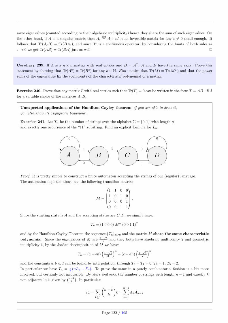
same eigenvalues (counted according to their algebraic multiplicity) hence they share the sum of such eigenvalues. On
the other hand, if A is a singular matrix then Aεdef= A + εI is an invertible matrix for any ε 6= 0 small enough. It
follows that Tr(AεB) = Tr(BAε), and since Tr is a continuous operator, by considering the limits of both sides as
ε→ 0 we get Tr(AB) = Tr(BA) just as well.
Corollary 239. If A is a n × n matrix with real entries and B = AT , A and B have the same rank. Prove this
statement by showing that Tr(Ak) = Tr(Bk) for any k ∈ N. Hint : notice that Tr(M) = Tr(MT ) and that the power
sums of the eigenvalues fix the coefficients of the characteristic polynomial of a matrix.
Exercise 240. Prove that any matrix T with real entries such that Tr(T ) = 0 can be written in the form T = AB−BAfor a suitable choice of the matrices A,B.
Unexpected applications of the Hamilton-Cayley theorem: if you are able to draw it,
you also know its asymptotic behaviour.
Exercise 241. Let Tn be the number of strings over the alphabet Σ = {0, 1} with length n
and exactly one occurrence of the “11” substring. Find an explicit formula for Ln.
Proof. It is pretty simple to construct a finite automaton accepting the strings of our (regular) language.
The automaton depicted above has the following transition matrix:
M =
1 1 0 0
1 0 1 0
0 0 0 1
0 0 1 1
.
Since the starting state is A and the accepting states are C,D, we simply have:
Tn = (1 0 0 0) Mn (0 0 1 1)T
and by the Hamilton-Cayley Theorem the sequence {Tn}n≥0 and the matrix M share the same characteristic
polynomial. Since the eigenvalues of M are 1±√
52 and they both have algebraic multiplicity 2 and geometric
multiplicity 1, by the Jordan decomposition of M we have:
Tn = (a+ bn)(
1+√
52
)n+ (c+ dn)
(1−√
52
)nand the constants a, b, c, d can be found by interpolation, through T0 = T1 = 0, T2 = 1, T3 = 2.
In particular we have Tn = 15 (nLn − Fn). To prove the same in a purely combinatorial fashion is a bit more
involved, but certainly not impossible. By stars and bars, the number of strings with length n− 1 and exactly k
non-adjacent 1s is given by(n−kk
). In particular:
Tn =∑k≥1
(n− kk
)k =
n−1∑k=1
AkAn−k
Page 122 / 195

8 REMARKABLE RESULTS IN LINEAR ALGEBRA
where Ak is the number of strings with length k, having no adjacent 1s and starting with a 1. By the convolu-
tion machinery the generating function of {Tn}n≥0 is simply given by the square of the generating function of
{An}n≥0 = {Fn+1}n≥0. The latter is a meromorphic function with two simple poles and we may recover the
previous closed form by partial fraction decomposition.
Exercise 242. (A) Let s be a non-empty string over the alphabet Σ = {0, 1}. Let As be the finite automaton
accepting the strings over Σ that do not contain s as a substring. Let us define Spec(s) as the spectrum of the
transition matrix of As. Investigate about the relations between Spec(s.t) and Spec(s),Spec(t), where . denotes
the concatenation of strings.
Exercise 243. (A) According to the notation introduced in the previous exercise, prove or disprove the existence
of a string s such that 2 cos 2π7 ∈ Spec(s).
Definition 244. We say that a weakly increasing sequence of real numbers a1 ≤ a2 ≤ . . . ≤ an interlaces another
weakly increasing sequence of real numbers b0 ≤ b1 ≤ . . . ≤ bn if
b0 ≤ a1 ≤ b1 ≤ a2 ≤ . . . ≤ an ≤ bn
holds.
Theorem 245 (Cauchy’s interlace Theorem). The eigenvalues of a Hermitian matrix A of order n are interlaced with
those of any principal submatrix of order n− 1.
Proof. Hermitian matrices have real eigenvalues. Let A be a Hermitian matrix of order n and let B be a principal
submatrix of A of order n − 1. If λn ≤ λn−1 ≤ . . . ≤ λ1 lists the eigenvalues of A and µn ≤ µn−1 ≤ . . . ≤ µ2 the
eigenvalues of B, we shall prove that
λn ≤ µn ≤ λn−1 ≤ µn−1 ≤ . . . ≤ λ2 ≤ µ2 ≤ λ1.
Proofs of this theorem have been based on Sylvester’s law of inertia and the Courant-Fischer min-max theorem.
Here we will give a simple, elementary proof of the theorem by using the intermediate value theorem.
Simultaneously permuting rows and columns, if necessary, we may assume that the submatrix B occupies rows 2, 3, . . . n
and columns 2, 3, . . . , n, so that A has the form
A =
(a y∗
y B
)
where ∗ stands for the conjugate transpose of a matrix. Let D = diag(µ2, µ3, . . . , µn). Then, since B is also Hermitian,
by the spectral Theorem there exists a unitary matrix U of order n − 1 such that U∗BU = D. Let U∗y = z =
(z2, z3, . . . , zn)T . We first prove the theorem for the special case where µn < µn−1 < . . . < µ3 < µ2 and zi = 0 for
i = 2, 3, . . . , n. Let
V =
(1 0T
0 U
)
Page 123 / 195

in which 0 denotes the zero vector. Then V is a unitary matrix and
V ∗AV =
(a z∗
z D
).
Let f(x) = det(xI − A) = det(xI − V ∗AV ), where I denotes the identity matrix. Expanding det(xI − V ∗AV ) along
the first row, we get
f(x) = (x− a)(x− µ2)(x− µ3) · · · (x− µn)−n∑i=2
fi(x)
where fi(x) = |zi|2(x − µ2) · · · (x− µi) · · · (x − µn) for i = 2, 3, . . . , n, with the hat-sign denoting a missing term.
We may notice that fi(µj) = 0 when j 6= i and fi(µi) is strictly positive or strictly negative according to i being,
respectively, even or odd. It follows that f(µi) is positive if i is odd and negative if i is even. Since f(x) is a
polynomial of degree n with positive leading coefficient, the intermediate value Theorem ensures the existence of n
roots λ1, λ2, . . . , λn of the equation f(x) = 0 such that λn < µn < λn−1 < µn−1 < . . . < λ2 < µ2 < λ1.
For the proof of the general case, let ε1, ε2, . . . be a sequence of positive real numbers such that εk is decreasing towards
zero, zi + εk 6= 0 for i = 2, 3, . . . , n and k = 1, 2, . . . and the diagonal entries of D + εkdiag(2, 3, . . . , n) are distinct for
fixed k. For k = 1, 2, . . . let
Ck =
(a z(εk)∗
z(εk) D(εk)
)where z(εk) = z + εk(1, 1, . . . , 1)T and D(εk) = D + εkdiag(2, 3, . . . , n), and let Ak = V CkV
∗. Then Ak is Hermitian
and Ak converges towards A. Let λ(k)n ≤ λ(k)
n−1 ≤ . . . ≤ λ(k)2 ≤ λ(k)
1 list the eigenvalues of Ak. Then
λ(k)n < µn + nεk < λ
(k)n−1 < µn−1 + (n− 1)εk < . . . < λ
(k)2 < µ2 + 2εk < λ
(k)1 .
Since λ(k)n , λ
(k)n−1, . . . , λ
(k)1 are n distinct roots of det(xI −Ak) = 0 for each k and since the graph of y = det(xI −Ak)
is sufficiently close to that of y = det(xI − A), it follows that the proof is complete by invoking the implicit function
Theorem:(λ
(k)n , λ
(k)n−1, . . . , λ
(k)1
)→ (λn, λn−1, . . . , λ1).
Theorem 246 (Sylvester’s criterion). A Hermitian matrix M is positive-definite
if and only if the determinants of the leading principal minors are positive.
Proof. If some minor has a negative or zero determinant the original matrix M cannot be positive definite by Cauchy’s
interlace theorem. This proves that the positivity of the mentioned determinants is a necessary condition. The converse
implication can be easily shown by induction on the dimension of M , or by exploiting the Cholesky decomposition
A = BTB with B being a non-singular matrix.
Page 124 / 195

9 THE FUNDAMENTAL THEOREM OF ALGEBRA
9 The Fundamental Theorem of Algebra
The purpose of this section is to shortly introduce some elements of Complex Analysis and use them to produce a
proof of the Fundamental Theorem of Algebra, stating that C is an algebraically closed field, or, in layman’s terms:
Theorem 247. Any non-constant p ∈ C[z] vanishes at some z ∈ C.
The first serious attempt to such problem is due to Gauss: it was mainly geometric, but it had a topological gap,
filled by Alexander Ostrowski in 1920. A rigorous proof was first published by Argand in 1806 (and revisited in 1813).
We will actually show many approaches and focus on geometric and analytic insights and their consequences. All
proofs below involve some analysis, or at least the topological concept of continuity of real or complex functions. Some
also use differentiable or even analytic functions. This fact has led to the remark that the Fundamental Theorem of
Algebra is neither fundamental, nor a theorem of algebra.
Definition 248. Suppose we are given a closed, oriented curve in the xy plane, not going through the origin. We
can imagine the curve as the path of motion of some object, with the orientation indicating the direction in which
the object moves. Then the winding number of the curve is equal to the total number of counterclockwise turns
that the object makes around the origin. When counting the total number of turns, counterclockwise motion counts
as positive, while clockwise motion counts as negative. For example, if the object first circles the origin four times
counterclockwise, and then circles the origin once clockwise, then the total winding number of the curve is three.
But given a closed curve γ : [0, 2π] → R2 \ {(0, 0)} represented by γ(t) = (x(t), y(t)) (which we may temporarily
assume to be smooth, too), how can we find its winding number around the origin? We may notice that in the open
first quadrant arctan y(t)x(t) gives an “angular displacement” with respect to the origin: in order to compute the winding
number of γ we just need to find a continuous determination of such angular displacement. For brevity we will not
delve into the theory of differential forms, we just mention that such continuous determination can be achieved through
a step of differentiation and a step of integration, namely:
d
dtarctan
y(t)
x(t)=
ddty(t)x(t)
1 + y(t)2
x(t)2
=x(t)y′(t)− y(t)x′(t)
x(t)2 + y(t)2
leading to
1
2π
∫ 2π
0
x(t)y′(t)− y(t)x′(t)
x(t)2 + y(t)2dt
as an expression for the winding number of γ around the origin. What if our curve is given by some f : S1 → C∗,with f being a holomorphic function? In such a case the previous winding number takes the following form:
1
2πi
∮|z|=1
f ′(z)
f(z)dz.
Now it comes an interesting remark, clarifying the interplay between winding numbers and zeroes of holomorphic
functions: in the previous line, the integrand function is formally ddz log f(z), hence if f = hg with h and g being
holomorphic functions, the winding number of f is just the sum between the winding number of h and the winding
number of g. It is very simple to check that for any m ∈ N the winding number of zm is exactly m and for every
w ∈ C\S1, by setting f(z) = z−w we get that the winding number of f is 1 or 0 according to |w| < 1 or |w| > 1: in the
first case f(S1) encloses the origin, in the latter it does not. Conversely, if f(z) is a holomorphic and non-vanishing
function over D, then f ′(z)f(z) is a holomorphic function over D and the integral
∮∂D
f ′(z)f(z) dz equals zero by Stokes’
theorem.
Page 125 / 195

Lemma 249. If f is a holomorphic function on D = {z ∈ C : |z| ≤ 1}, non-vanishing over ∂D,
Nf =1
2πi
∮∂D
f ′(z)
f(z)dz
equals the number of zeroes of f in D, counted according to their multiplicity.
This Lemma can be seen both as a consequence of the residue Theorem or as a remark in Differential Geometry that
can be used to prove the residue Theorem. Such Lemma has a crucial role in the usual proof of the Jordan curve
Theorem, since it gives that a smooth, simple and closed curve cannot partition R2 in more than two connected
components. A curve fulfilling such constraints splits R2 in at least two connected components by the existence of
a tubular neighbourhood, then the chance to drop the previous smoothness assumption is granted by invoking Sard’s
Theorem.
Theorem 250 (The double leash principle). Assume that you are connected to a thin tree by a leash of fixed length
L. Assume that you dog is connected to you by a leash of fixed length l < L. If you take a walk and after some time
you return at your starting point, your winding number around the tree and your dog’s are the same.
The above statement is usually known as Rouche Theorem. We opted for such fancy introduction since we believe
the previous formulation might help the reader to grasp the geometric idea faster and better. In a more rigorous way:
Theorem 251 (Rouche). If f(z) and f(z) + g(z) are holomorphic function on the closed unit disk D centered at the
origin, and for every z ∈ ∂D we have 0 < |g(z)| < |f(z)|, then f and f + g have the same number of zeros inside D,
where each zero is counted as many times as its multiplicity. The same holds if D is replaced by some compact region
K whose boundary ∂K is a simple, piecewise-smooth and closed curve.
Proof. We have already shown that the wanted number of zeroes is given by a winding number. Since for any z ∈ ∂Dwe may write
f(z) + g(z) = f(z)
(1 +
g(z)
f(z)
)the winding number of f + g is given by the sum between the winding number of f and the winding number of the
curve
h : S1 → C∗, h(eiθ)def= 1 +
g(eiθ)
f(eiθ).
However, the winding number of h is clearly zero, since h stays “on the right” of the origin. As a matter of fact,∣∣∣∣ g(z)
f(z)
∣∣∣∣is a continuous function on a compact set (S1) attaining a maximum M < 1, hence Re(h) ≥ 1−M > 0 by the triangle
inequality. It follows that f and f + g have the same winding number, hence the same number of zeroes in D.
We are ready to prove the following statement:
Lemma 252. The Fundamental Theorem of Algebra is a simple consequence of the double leash principle.
Page 126 / 195

9 THE FUNDAMENTAL THEOREM OF ALGEBRA
Proof. We may assume without loss of generality that
p(z) = zn + an−1zn−1 + . . .+ a0 ∈ C[z]
is a monic polynomial with degree n ≥ 1 and p(0) = a0 6= 0. Our purpose is to prove it has a zero somewhere.
We prove first that if it has a zero, it cannot be too far from the origin. Let us consider
M = 1 + |an−1|+ . . .+ |a0|
and show that |z| ≥M implies p(z) 6= 0. Since M > 1, for any z ∈ C such that |z| ≥M we have:
∣∣an−1zn−1 + . . .+ a0
∣∣ ≤ |an−1||z|n−1 + . . .+ |a0| ≤ (|an−1|+ . . .+ |a0|) |z|n−1 = (M − 1)|z|n−1 < |z|n
hence p(z) = 0 cannot occur, since it would imply |z|n =∣∣an−1z
n−1 + . . .+ a0
∣∣. This proves all the complex zeroes of p,
if existing, lie in the region |z| < M . But the inequality above also shows that f(z) = zn and g(z) = an−1zn−1+. . .+a0
meet the hypothesis of Rouche’s Theorem for the the region K = {z ∈ C : |z| ≤ M}. In particular the number of
zeroes of p(z) = f(z) + g(z) in K equals the number of zeroes of f(z) = zn in K and we are done:
p(z) has exactly n zeroes in the region |z| < M, counted according to their multiplicity.
The inclusion
{z ∈ C : p(z) = 0} ⊂ {z ∈ C : |z| ≤M}
can also be proved by applying the Gershgorin circle Theorem to the companion matrix of p.
Exercise 253. Prove that for any n ≥ 5 the polynomial
pn(z) = zn + z + 1
has approximately n3 roots in in the region |z| ≤ 1, with an error
not greater than one.
Sketch of proof. If n ≡ 2 (mod 3) the primitive third roots of
unity ω, ω2 are also roots of pn. Conversely, if we denote as D
the unit disk centered at the origin, we may notice that ∂D and
−(∂D + 1) intersect only at ω, ω2: it follows that the n ≡ 2
(mod 3) case is the only case in which pn(z) has roots at ∂D.
The number of roots we want to approximate is given by the
winding number of the curve γn : [0, 2π]→ C, γn(θ) = pn(eiθ).
The diagram to the right depicts the n = 13 case, for instance.The graph of e13iθ + eiθ + 1 for θ ∈ [0, 2π].
Page 127 / 195
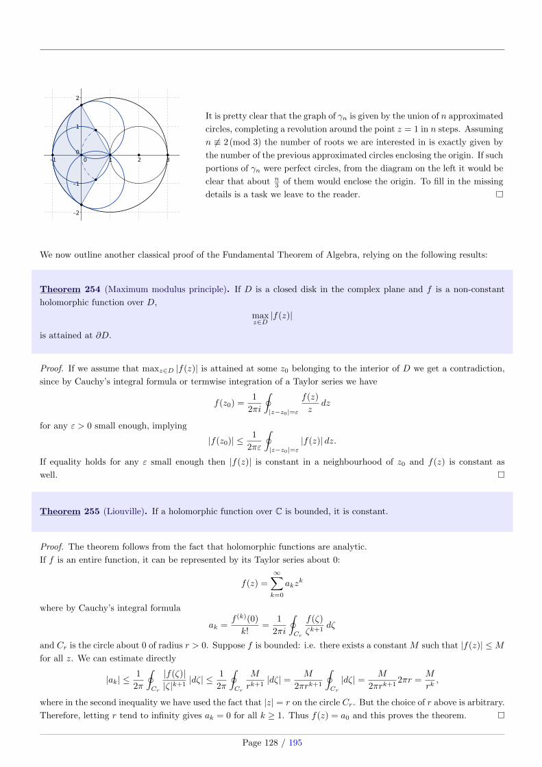
It is pretty clear that the graph of γn is given by the union of n approximated
circles, completing a revolution around the point z = 1 in n steps. Assuming
n 6≡ 2(mod 3) the number of roots we are interested in is exactly given by
the number of the previous approximated circles enclosing the origin. If such
portions of γn were perfect circles, from the diagram on the left it would be
clear that about n3 of them would enclose the origin. To fill in the missing
details is a task we leave to the reader.
We now outline another classical proof of the Fundamental Theorem of Algebra, relying on the following results:
Theorem 254 (Maximum modulus principle). If D is a closed disk in the complex plane and f is a non-constant
holomorphic function over D,
maxz∈D|f(z)|
is attained at ∂D.
Proof. If we assume that maxz∈D |f(z)| is attained at some z0 belonging to the interior of D we get a contradiction,
since by Cauchy’s integral formula or termwise integration of a Taylor series we have
f(z0) =1
2πi
∮|z−z0|=ε
f(z)
zdz
for any ε > 0 small enough, implying
|f(z0)| ≤ 1
2πε
∮|z−z0|=ε
|f(z)| dz.
If equality holds for any ε small enough then |f(z)| is constant in a neighbourhood of z0 and f(z) is constant as
well.
Theorem 255 (Liouville). If a holomorphic function over C is bounded, it is constant.
Proof. The theorem follows from the fact that holomorphic functions are analytic.
If f is an entire function, it can be represented by its Taylor series about 0:
f(z) =
∞∑k=0
akzk
where by Cauchy’s integral formula
ak =f (k)(0)
k!=
1
2πi
∮Cr
f(ζ)
ζk+1dζ
and Cr is the circle about 0 of radius r > 0. Suppose f is bounded: i.e. there exists a constant M such that |f(z)| ≤Mfor all z. We can estimate directly
|ak| ≤1
2π
∮Cr
|f(ζ)||ζ|k+1
|dζ| ≤ 1
2π
∮Cr
M
rk+1|dζ| = M
2πrk+1
∮Cr
|dζ| = M
2πrk+12πr =
M
rk,
where in the second inequality we have used the fact that |z| = r on the circle Cr. But the choice of r above is arbitrary.
Therefore, letting r tend to infinity gives ak = 0 for all k ≥ 1. Thus f(z) = a0 and this proves the theorem.
Page 128 / 195
9 THE FUNDAMENTAL THEOREM OF ALGEBRA
Corollary 256 (Casorati-Weierstrass). If f is a non-constant entire function, then its image is dense in C.
Proof. If the image of f is not dense, then there is a complex number w and a real number r > 0 such that the open
disk centered at w with radius r has no element of the image of f . Define g(z) = 1f(z)−w . Then g is a bounded entire
function, since
∀z ∈ C, |g(z)| = 1
|f(z)− w|<
1
r
So, g is constant, and therefore f is constant.
Corollary 257. If p(z) ∈ C[z] is a monic polynomial with degree n ≥ 1 and p(0) 6= 0, it has a complex root.
Proof. Since |p(z)| → +∞ as |z| → +∞, there is some closed disk D centered at the origin such that |p(z)| > |p(0)|for any z outside D. Assuming that p(z) is non-vanishing, it follows that minz∈C |p(z)| is attained at some z0 ∈ Dand q(z) = 1
p(z) is an entire function such that
∀z ∈ C, |q(z)| ≤ 1
|p(z0)|.
By Liouville’s Theorem we get that both q and p are constant functions, leading to a contradiction.
A shortened proof. Assume that p(z) = zn + an−1zn−1 + . . . + a0 ∈ C[z] with n ≥ 1 is non-vanishing over C.
By the residue Theorem, for any r > 0 we have that∮|z|=r
dz
z p(z)=
2πi
p(0)6= 0
but the limit of the LHS as r → +∞ is clearly 0.
Theorem 258 (Open mapping Theorem). Any non-constant holomorphic function on C is an open map,
i.e. it sends open subsets of C to open subsets of C.
Proof. Assume f : U → C is a non-constant holomorphic function and U is a domain of the complex plane. We have
to show that every point in f(U) is an interior point of f(U), i.e. that every point in f(U) has a neighbourhood (open
disk) which is also in f(U). Consider an arbitrary w0 in f(U). Then there exists a point z0 in U such that w0 = f(z0).
Since U is open, we can find d > 0 such that the closed disk B around z0 with radius d is fully contained in U .
Consider the function g(z) = f(z)−w0. Note that z0 is a root of the function. We know that g(z) is not constant and
holomorphic. The roots of g are isolated by the identity theorem, and by further decreasing the radius of the image
disk d, we can assure that g(z) has only a single root in B (although this single root may have multiplicity greater
than 1). The boundary of B is a circle and hence a compact set, on which |g(z)| is a positive continuous function, so
the extreme value Theorem guarantees the existence of a positive minimum e, that is, e is the minimum of |g(z)| for
z on the boundary of B and e > 0. Denote by D the open disk around w0 with radius e. By Rouche’s theorem, the
function g(z) = f(z)−w0 will have the same number of roots (counted with multiplicity) in B as h(z)def= f(z)−w1 for
any w1 in D. This is because h(z) = g(z) + (w0 −w1), and for z on the boundary of B, |g(z)| ≥ e ≥ |w0 −w1|. Thus,
for every w1 in D, there exists at least one z1 in B such that f(z1) = w1. This means that the disk D is contained in
f(B). The image of the ball B, f(B), is a subset of the image of U , f(U). Thus w0 is an interior point of f(U). Since
w0 was arbitrary in f(U) we know that f(U) is open. Since U was arbitrary, the function f is open.
Lemma 259. Any non-constant polynomial p(z) ∈ C[z] is a closed map.
Proof. We have that |p(z)| → +∞ as |z| → +∞. Suppose that p(zk) → w ∈ C as k → +∞: then {zk} is bounded,
so taking a subsequence if necessary, there is z ∈ C such that zk → z. By continuity p(zk) → p(z), concluding that
w = p(z).
Page 129 / 195

Corollary 260. If p(z) ∈ C[z] is a non-constant polynomial, p(C) is unbounded and simultaneously open and closed.
If follows that p(C) = C, i.e. any non-constant polynomial with complex coefficients is surjective. In particular there
is at least a complex solution of p(z) = 0.
Exercise 261. Given a non-constant polynomial p(z) ∈ C[z] such that p(0) 6= 0, prove that the following statements
are equivalent forms of the Fundamental Theorem of Algebra:
1. The companion matrix of p has at least an eigenvector in Cn;
2. q(z) = 1p(z) is an analytic function in a neighbourhood of the origin with a finite radius of convergence;
3. If p is the characteristic polynomial of a recurrent sequence {an}n≥0, for some M ∈ R+
the following limit does not exist:
limn→+∞
n∑k=0
akMk.
An interesting part of Complex Analysis is related to the problem of extending Rolle’s Theorem (if f is a differentiable
function on [a, b] and f(a) = f(b) = 0 holds, there is some ξ ∈ (a, b) such that f ′(ξ) = 0) to the complex case.
Theorem 262 (Gauss-Lucas). If ζ1, . . . , ζn ∈ C (n ≥ 3) are the roots of a polynomial p(z) ∈ C[z],
all the roots of p′(z) lie inside the convex hull of ζ1, . . . , ζn.
Proof. We may assume without loss of generality that p(z) is a monic polynomial with simple roots. Then by
considering the logarithmic derivative of p(z) we have the following identity
p′(z) = p(z)
n∑k=1
1
z − ζk
and p′(z) vanishes iff s(z) =∑nk=1
1z−ζk vanishes, since p(z) and p′(z) have no common root. Let us assume that s(z)
vanishes at a point w lying outside the convex hull of ζ1, . . . , ζk, or on its boundary. By the Hann-Banach theorem
there is some line ` through the origin such that all the vectors w − ζ1, . . . , w − ζk lie on the same side of `. By
conjugation, the same applies to the vectors 1w−ζ1 , . . . ,
1w−ζk , hence for some θ ∈ R the complex number eiθs(w) has
a non-zero real/imaginary part. s(w) 6= 0 leads to a contradiction, completing the proof.
About cubic polynomials, a remarkable and way sharper result is well-known:
Theorem 263 (Marden). If A,B,C are three distinct points in the
complex plane and we denote as D,E the roots of
d
dz(z −A)(z −B)(z − C),
then D,E are the foci of the Steiner inellipse of ABC, centered atA+B+C
3 and tangent to the sides of ABC at their midpoints.
What is the best possible improvement of the Gauss-Lucas Theorem still is an open problem in the general case.
The following result has only been proved for polynomials having degree ≤ 8 and for some other special cases:
Page 130 / 195

9 THE FUNDAMENTAL THEOREM OF ALGEBRA
The Ilieff-Sendov conjecture. If all the zeros of a polynomial p(z) lie in ‖z‖ ≤ 1 and if r is a zero of p(z),
then there is a zero of p′(z) in the disk ‖z − r‖ ≤ 1.
Exercise 264. By exploiting the Gauss-Lucas theorem, show that the following entire functions only have real zeroes:
sin(z) +√
2 sin(z√
2), Si(z) =∑n≥0
(−1)nz2n+1
(2n+ 1) · (2n+ 1)!, J0(z) =
∑n≥0
(−z2)n
4nn!2.
Exercise 265. By exploiting the Gauss-Lucas theorem, show that for any λ ∈ [1,+∞) all the solutions of
cot(x) + λx = 0 are real numbers.
Yet another way for approaching Calculus. The exponential function is usually introduced by proving that
limn→+∞(1 + 1
n
)nexists, then showing that ex
def= limn→+∞
(1 + x
n
)nis a differentiable function, then noticing
that ddxe
x = ex leads to very-known Taylor series and to De Moivre’s formula. Here we outline a different way for
approaching the early stages of Calculus.
1. One may directly introduce the complex exponential function through an everywhere-convergent power
series,
∀z ∈ C, ezdef=∑n≥0
zn
n!,
2. then check through the convolution machinery that such function fulfills ea · eb = ea+b for any a, b ∈ C;
3. In particular, for any θ ∈ R we have that eiθ ∈ S1, since |eiθ|2 = eiθ · e−iθ = 1
4. and the map γ : R → S1 given by γ(θ) = eiθ is a parametrization of S1 with constant speed, since by the
series definition ddθ e
iθ = ieiθ and the last quantity has unit modulus by the previous point (Pythagorean
Theorem);
5. Since γ is an arc-length parametrization of S1, we may define sin(θ) and cos(θ) through
sin(θ)def= Im eiθ, cos(θ)
def= Re eiθ
and derive the addition formulas for sin and cos from the point (2.);
6. Since γ travels S1 counter-clockwise, by defining π as
πdef= inf
{θ ∈ R+ : sin(θ) = 0
}we get that π equals half the length of the unit circle, or, equivalently, the area of the unit circle.
Additionally, eiπ + 1 = 0;
7. By the previous points ez is an entire function and a solution of the differential equation f ′(z) = f(z);
8. By the series definition it also follows that
sin(z) =∑n≥0
(−1)n
(2n+ 1)!z2n+1, cos(z) =
∑n≥0
(−1)n
(2n)!z2n
are entire functions and solutions of the differential equation f ′′(z) + f(z) = 0;
Page 131 / 195
9. From the Pythagorean Theorem sin2 θ + cos2 θ = 1, hence
π = 2
∫ 1
0
dx√1− x2
x 7→√u
=
∫ 1
0
du√u(1− u)
symmetry= 4
∫ 1/√
2
0
dx√1− x2
and by integrating termwise the Taylor series of 1√1−x2
we get the following series representation for π:
π = 2√
2∑n≥0
(2nn
)8n(2n+ 1)
= 3.1415926535897932384626433832795 . . .
As an alternative, the integral of√
1− x2 over some sub-interval of [−1, 1] is clearly related with the area of
a circle sector. By computing a Taylor series and applying termwise integration again, we may easily derive
Newton’s identity
π = 4− 4∑n≥1
(2nn
)(4n2 − 1)4n
.
Exercise 266. Prove that for any n ∈ N the following identity holds:
S(n) =
n∑k=0
2k(
2n− kn
)= 4n.
Proof.
S(n) =
n∑k=0
2n−k(n+ k
n
)is the coefficient of xn in the product between
∑k≥0 2kxk = 1
1−2x (geometric series) and∑k≥0
(n+kn
)xk = 1
(1−x)n+1
(stars and bars). In particular
S(n) = Res
(1
(1− 2x) [x(1− x)]n+1 , x = 0
)but due to the symmetry of the meromorphic function 1
(1−2x)[x(1−x)]n+1 the residue at 0 and the residue at 1 are the
same number. The only other pole is at x = 12 and the sum of the residues is zero, hence S(n) = 4n can be proved
from the straightforward
Res
(1
(1− 2x) [x(1− x)]n+1 , x =
1
2
)= −2 · 4n.
Page 132 / 195

10 QUANTITATIVE FORMS OF THE WEIERSTRASS APPROXIMATION THEOREM
10 Quantitative forms of the Weierstrass approximation Theorem
In a previous section about Chebyshev and Legendre polynomials we have already seen a brilliant proof of Weierstrass
approximation Theorem, where the problem of finding uniform polynomial approximations for continuous functions
has been reduced to finding uniform polynomial approximations for a single function, namely |x|. In the current
section we will investigate about a fascinating subject: by fixing some interval [a, b] ⊂ R and recalling that ‖f−g‖∞ =
supx∈[a,b] |f(x)− g(x)|, we ask:
Given a function f ∈ C0[a, b], let us denote as pN (x) the polynomial with degree n minimizing ‖f − pN‖∞.
Is there some relation between the regularity of f and the speed of convergence towards zero for ‖f − pN‖∞,
as N → +∞?
Our main goal is to prove the following results:
Theorem 267 (Bernstein). If f : [0, 2π]→ C is a 2π-periodic function, n is a natural number, α ∈ (0, 1)
and for some constant C(f) > 0 the sequence of trigonometric polynomials {Pn(x)}n≥0 fulfills
∂Pn = n, ∀n ≥ 1, ‖f − Pn‖∞ ≤C(f)
nr+α
then f(x) = P0(x) + ϕ(x), where ϕ(x) is a function of class Cr on the interval (0, 2π) and ϕ(r)(x)
is a α-Holder continuous function.
Theorem 268 (Jackson). If f : [0, 2π]→ C is a 2π-periodic function of class Cr such that∣∣f (r)(x)
∣∣ ≤ 1
for any x ∈ [0, 2π], there exists a sequence {Pn(x)}n≥1 of trigonometric polynomials such that:
∂Pn = n, ‖f − Pn‖∞ ≤C(r)
nr
where C(r) only depends on r, and it is the Akhiezer-Krein-Favard constant C(r) = 4π
∑k≥0
(−1)k(r+1)
(2k+1)r+1 .
In other terms, the degree of regularity of a function is exactly given by the speed of convergence towards zero of the
uniform error for the optimal polynomial approximations with respect to the infinity-norm. The Bernstein Theorem
follows from Bernstein’s inequality, stating:
Theorem 269 (Bernstein’s inequality). If P (z) is a polynomial with complex coefficients and degree n,
max|z|≤1
|P ′(z)| ≤ n ·max|z|≤1
|P (z)|
from which it follows that:
max|z|≤1
∣∣∣P (k)(z)∣∣∣ ≤ n!
(n− k)!·max|z|≤1
|P (z)| .
Jackson’s Theorem, instead, follows from a projection technique in L2 very similar to the one we saw when computing
the Fourier-Chebyshev expansion for |x|. Our path starts by presenting Bernstein’s proof of Weierstrass approximation
Theorem, dating back to 1912. If f is a continuous function on the interval [0, 1], the sequence of polynomials defined
through
(Bn(f)) (x) =
n∑k=0
(n
k
)xk(1− x)n−kf
(k
n
)
Page 133 / 195

is uniformly convergent towards f . An interesting remark is that we need to prove the claim only for the following
cases: f0(x) = 1, f1(x) = x and f2(x) = x2. Indeed we have Bn(f0) = f0, Bn(f1) = f1 and Bn(f2) =(1− 1
n
)f2 + 1
nf1.
Moreovern∑k=0
(k
n− x)2(
n
k
)xk(1− x)n−k =
x(1− x)
n≤ 1
4n
and by considering some δ > 0 and by defining F as the set of ks in {0, . . . , n} such that∣∣ kn − x
∣∣ ≥ δ, we have:
∑k∈F
(n
k
)xk(1− x)n−k ≤ 1
δ2
∑k∈F
(k
n− x)2(
n
k
)xk(1− x)n−k
≤ 1
δ2
n∑k=0
(k
n− x)2(
n
k
)xk(1− x)n−k ≤ 1
4nδ2.
Since f is a continuous function on a compact set, it is uniformly continuous, hence there is some δ > 0 which ensures
|f(x)− f(y)| ≤ ε2 as soon as |x− y| < δ. Since
(nk
)xk(1− x)n−k are non-negative numbers adding to 1,
|f(x)−Bn(f)(x)| =
∣∣∣∣∣f(x)−n∑k=0
f
(k
n
)(n
k
)xk(1− x)n−k
∣∣∣∣∣=
∣∣∣∣∣n∑k=0
[f(x)− f
(k
n
)](n
k
)xk(1− x)n−k
∣∣∣∣∣≤
n∑k=0
∣∣∣∣f(x)− f(k
n
)∣∣∣∣ (nk)xk(1− x)n−k.
If now we fix n (how will be clear soon) and denote ‖f‖ = maxx∈[0,1] |f(x)|, by naming as F the set of ks such that
|x− k/n| ≥ δ, we have |f(x)− f(k/n)| ≤ ε2 for any k in the complement of F and |f(x)− f(k/n)| ≤ 2‖f‖ in general.
It follows that:
|f(x)−Bn(f)(x)| ≤∑k∈F
∣∣∣∣f(x)− f(k
n
)∣∣∣∣ (nk)xk(1− x)n−k +
∑k 6∈F
∣∣∣∣f(x)− f(k
n
)∣∣∣∣ (nk)xk(1− x)n−k
≤ 2‖f‖∑k∈F
(n
k
)xk(1− x)k +
ε
2
∑k 6∈F
(n
k
)xk(1− x)n−k
≤ ‖f‖2nδ2
+ε
2
and the last term is smaller than ε as soon as n > ‖f‖εδ2 . A remarkable feature of Bernstein’s approach is that the
properties Bn(αf + βg) = αBn(f) + βBn(g) and Bn(f) ≥ 0 if f ≥ 0 are enough to lead to a generalization:
Theorem 270 (Bohman, Korovkin, 1952). Assuming that Tn : C0[0, 1]→ C0[0, 1] is a sequence of linear and positive
operators, such that Tn(f) is uniformly convergent to f in each one of the following cases
f0(x) = 1, f1(x) = x, f2(x) = x2,
then Tn(f) is uniformly convergent to f for any f ∈ C0[0, 1].
This result already allows to outline a sketch of proof for Jackson’s Theorem: let us assume that f is a function of
class Cr, 2π-periodic. In order to approximate f through trigonometric polynomials, the key idea is to approximate
f (r) first, then exploit repeated termwise integration. By setting g = f (r), a natural approach we may follow is to
consider a truncation of the Fourier series of g, i.e. to consider a convolution between g and Dirichlet’s kernel DN .
However, Dirichlet’s kernel is not positive or bounded with respect to the L1-norm (this is the main reason fo the
Page 134 / 195

10 QUANTITATIVE FORMS OF THE WEIERSTRASS APPROXIMATION THEOREM
Gibbs phenomenon to arise in peculiar situations), hence the initial naive idea requires to be fixed. In particular,
instead of considering truncations of Fourier series, it is better to consider suitably weigthed Fourier series. The map:
g(θ) =∑n∈Z
cneniθ −→ g(θ) =
N∑n=−N
(1− |n|
N
)cne
inθ
follows the idea of approximating g through the convolution between g and the Fejer kernel FN . This kernel is positive
and concentrated around the origin, hence g ∗ FN is uniformly convergent to g on the interval [0, 2π]. In order to
achieve a better control on error with respect to the L2-norm, a more efficient way is to approximate g through the
convolution between g and the square of Fejer kernel, also known as Jackson’s kernel. By squaring the positivity
of such kernel is preserved, and it becomes more concentrated around the origin. Repeated termwise integration
then leads to Jackson’s theorem in a quite straightforward way. The Akhiezer-Krein-Favard constant comes from the
fact that among the 2π-periodic and continuous functions, the triangle wave is in some sense the worst approximable
function through such convolution trick, but we already computed the Fourier-Chebyshev expansion of the triangle
wave.
As an alternative, it is not terribly difficult to prove the following statement, that follows by combining Lagrange
interpolation with properties of Chebyshev polynomials:
Theorem 271. If f(x) is a function of class Cn+1 on the interval [−1, 1] and Cn(f) is the Lagrange interpolating
polynomial for f , with respect to the points given by the roots of the Chebyshev polynomial Tn+1 (also known as
Chebyshev nodes), we have:
|f(x)− Cn(f)(x)| ≤∥∥f (n+1)
∥∥2n(n+ 1)!
.
Additionally, we have that:
Lemma 272. If p(x) is a real polynomial with degree ≤ (n− 1), we have:
p(x) =
n∑k=1
p(xk)(−1)k−1√
1− x2k
Tn(x)
x− xk
with x1, . . . , xn being the roots of Chebyshev polynomial Tn(x).
In this case, indeed, Lagrange interpolation leads to an identity, not only an approximation.
Under the same assumptions we also have:
maxx∈[−1,1]
|p(x)| ≤ n maxx∈[−1,1]
∣∣∣√1− x2 p(x)∣∣∣ = M.
If x ∈ [xn, x1], i.e. if |x| ≤ cos π2n , we have
√1− x2 ≥ sin π
2n ≥1n , so such inequality is trivial.
On the other hand, if all the terms (x− xk) have the same sign, we have:
|p(x)| ≤ M
n2
∣∣∣∣∣n∑k=1
Tn(x)
x− xk
∣∣∣∣∣ =M
n2|T ′n(x)| ≤M.
By enforcing the substitution x→ cos θ, we have that if S(θ) is an odd trigonometric polynomial
having degree n, then:
maxθ∈[0,2π]
∣∣∣∣S(θ)
sin θ
∣∣∣∣ ≤ n maxθ∈[0,2π]
|S(θ)| .
Page 135 / 195

We are ready to prove Bernstein’s inequality. If S(θ) is a trigonometric polynomial with degree n, we may define the
auxiliary function
f(α, θ) =S(α+ θ)− S(α− θ)
2
and this function (with respect to θ) is an odd trigonometric polynomial with degree ≤ n. Due to previous results,
maxθ∈[0,2π]
∣∣∣∣f(α, θ)
sin θ
∣∣∣∣ ≤ n maxθ∈[0,2π]
|f(α, θ)| ≤ n maxθ∈[0,2π]
|S(θ)| .
However
S′(α) = limθ→0
S(α+ θ)− S(α− θ)2θ
= limθ→0
f(α, θ)
sin θ
hence for any α, |S′(α)| ≤ nmaxθ∈[0,2π] |S(θ)| as wanted.
By reversing the previous substitution, we also get:
Theorem 273 (Markov brothers’ inequality). If p(x) is a real polynomial with degree n,
maxx∈[−1,1]
| p′(x)| ≤ n2 maxx∈[−1,1]
|p(x)| .
We now prove a minor version of Bernstein’s Theorem:
Lemma 274. If f is a 2π-periodic function and for some α ∈ (0, 1) the given function can be approximated through
trigonometric polynomials with degree n, where the uniform error of such approximations is ≤ Anα , then f is an
α-Holderian continuous function.
Proof. For any n ≥ 1, we may pick a trigonometric polynomial Sn such that ‖f − Sn‖ ≤ Anα . In particular, {Sn}n≥1
is uniformly convergent. With the assumptions V0 = S1 and Vn = S2n − S2n−1 , Vn turns out to be a trigonometric
polynomial having degree ≤ 2n and fulfilling f =∑n≥0 Vn. Indeed we have
‖Vn‖ ≤ ‖S2n − f‖+ ‖S2n−1 − f‖ ≤ A(2−nα + 2α−nα
)≤ B · 2−nα
and the RHS is summable, hence∑n≥0 Vn is uniformly convergent to f . The key idea is now to approximate
|f(x)− f(y)| through a finite number of Vns, number to suitably fix later.
|f(x)− f(y)| ≤∑n≥0
|Vn(x)− Vn(y)|
≤m−1∑n=0
|Vn(x)− Vn(y)|+ 2∑n≥m
‖Vn‖
= |x− y|m−1∑n=0
|V ′n(ξn)|+ 2B∑n≥m
2−nα
Bern≤ |x− y|
m−1∑n=0
2n ‖Vn‖+ 2B∑n≥m
2−nα
≤ C[|x− y| 2m(1−α) + 2−mα
].
We want the last term to be bounded by |x− y|α, i.e., by setting δ = |x− y|, we want the following inequality to hold:
(2mδ)1−α + (2mδ)α ≤ D
and for such a purpose it is enough to choose m in such a way that 1 < 2mδ < 2 is granted.
Page 136 / 195

11 ELLIPTIC INTEGRALS AND THE AGM
Bernstein’s theorem, as presented at the beginning of this section, is a simple generalization of the last statement. There
is a non-trivial subtlety: one might conjecture that if f is a 2π-periodic function, admitting approximations through
trigonometric polynomials with degree n, whose uniform error is ≤ An , then f is a Lipschitz-continuous function.
However that is not the case: we may state, at best, that such assumptions and |x− y| ≤ δ grant |f(x)− f(y)| ≤Kδ |log δ| for any δ small enough. Essentially, a form of Gibbs phenomenon arises in the proof of Bernstein’s Theorem,
too.
At last we mention an interesting strengthening of Weierstrass approximation Theorem, which can be interpreted as
a deep result for dealing with lacunary Fourier series, or as a deep result in the theory of interpolation.
Theorem 275 (Muntz). If 0 = λ0, λ1, λ2, . . . is an increasing sequence of natural numbers, the subspace of C0[0, 1]
spanned by xλ0 , xλ1 , xλ2 , . . . is dense in C0[0, 1] if and only if the series∑n≥1
1λn
is divergent.
Exercise 276 (Chebyshev equioscillation theorem). Let f be a continuous function on the interval [a, b].
Prove that among the polynomials p ∈ R[x] having degree ≤ n, the polynomial minimizing ‖p− f‖∞ fulfills
p(xk)− f(xk) = σ(−1)k‖p− f‖∞
at n+ 2 points a ≤ x0 < x1 . . . < xn ≤ b with σ ∈ {−1,+1}.
Exercise 277. f(x) = ax3 + bx2 + cx+ d is a polynomial with real coefficients fulfilling the following property:
∀x ∈ [0, 1], |f(x)| ≤ 1.
Prove that |a|+ |b|+ |c|+ |d| ≤ 99 holds and that such inequality is optimal, i.e. 99 cannot be replaced by any smaller
number.
11 Elliptic integrals and the AGM
The flourishing theory of elliptic integrals started its development at the beginning of the nineteenth century, especially
thanks to Niels Henrik Abel, whose work was really appreciated by Carl Gustav Jacob Jacobi (“Abel teaches us: you
always have to consider an inversion!”). Jacobi gave significant contributions to the theory of elliptic integrals,
leading to the foundations of the modern theory of modular forms. In Physics elliptic integrals arise, for instance, in
the determination of the exact period of a pendulum.
Let us assume to have a mass-m point at one end of a massless, inextensible rod of length l, with the other end hinged
at fixed point. Let us denote as θ the angle between the position of the pendulum and the equilibrium point, in a
frictionless environment with a constant gravitational acceleration in the same direction. The mechanical energy of
the pendulum equals
mgl(1− cos θ) +ml2
2θ2 = E
and this quantity is time-invariant. The instants such that θ = 0 give the amplitude of oscillations, and by assuming
E ≤ mgl (i.e. by assuming the pendulum has not enough energy to go above the hinge) we have:
θmax = 2 arcsin
√E
2mgl.
Page 137 / 195

The conservation of mechanical energy allows us to write a differential equation for θ:
dθ
dt=
√2E
ml2− 2g
l(1− cos θ)
from which it follows that time can be written as a function of θ, and in particular:
T = 4
∫ θmax
0
dθ√2Eml2 −
2gl (1− cos θ)
= 4
√l
g
∫ 1
0
du√(1− u2)
(1− Eu2
2mgl
) = 4
√l
g
∫ π/2
0
dϕ√1− E sin2 ϕ
2mgl
.
For small energies an accurate approximation of the period is thus given by:
4
√l
g
∫ 1
0
du√1− u2
= 2π
√l
g
and the pendulum is approximately isocronous (the time needed to complete an oscillation does not depend on the
amplitude of such oscillation, just like in the idea harmonic oscillator described by the differential equation x+ gl x = 0).
In a exact form, by setting κ2 = E2mgl :
T = 4
√l
g
∫ π/2
0
dϕ√1− κ2 sin2 ϕ
= 2π
√l
g
1 +∑m≥1
((2m
m
)1
4m
)2κ2m
4
≤ 2π
√l
g
[1− 1
4πlog(1− κ2)
].
we get that an approximation of the period that is much more accurate than 2π√
lg , also for non-negligible values of
E, is provided by:
T ≈ 2π
√l
g
[1 +
log(1− κ2)
16
]= 2π
√l
g
[1 +
log cos θmax2
8
].
In particular, the exact period of a pendulum is given by a complete elliptic integral of the first kind.
The adjective elliptic has probably been chosen for a geometric reason: let E be an ellipse described by the equationx2
a2 + y2
b2 = 1, with major axis 2a, minor axis 2b, semi-focal distance c =√a2 − b2 and eccentricity e = c
a . Since any
affine map preserves the ratios of areas, the area of E equals πab. Let us denote as L(a, b) the ellipse perimeter. By
the integral formula for computing the length of a C1 curve we have:
L(a, b) = 4
∫ π/2
0
√a2 sin2 θ + b2 cos2 θ dθ = 4a
∫ π/2
0
√1 + e2 sin2 θ dθ.
In particular, the ellipse perimeter is given by a complete elliptic integral of the second kind.
Let us denote as Mp(a, b) the order-p mean between a and b, i.e.:
Mp(a, b) =p
√ap + bp
2.
Theorem 278.
M1(a, b) ≤ L(a, b)
2π≤M2(a, b).
Proof. By the concavity of the logarithm function we have√x+√y ≤
√2(x+ y), from which:
L(a, b) = 4
∫ π/4
0
√a2 sin2
(π4− θ)
+ b2 cos2(π
4− θ)
+
√a2 sin2
(π4
+ θ)
+ b2 cos2(π
4+ θ)dθ
≤ 4
∫ π/4
0
√2(a2 + b2) dθ = 2π ·M2(a, b).
Page 138 / 195

11 ELLIPTIC INTEGRALS AND THE AGM
The first inequality, despite its appearance, is actually more difficult to prove.
We may use the following identity as a starting point:
L(a, b) = (a+ b)
∫ π
0
√1 +
(a− ba+ b
)2
+ 2
(a− ba+ b
)cos(2θ) dθ.
Since 1 + x2 + 2x cos(2θ) = (1− x e2iθ) · (1 + x e−2iθ) we have:∫ π
0
√1 + x2 + 2x cos(2θ) dθ =
∫ π
0
√(1− x e2iθ) · (1 + x e−2iθ) dθ
=
∫ π
0
∑m,n≥0
1
(2m− 1)(2n− 1)· 1
4m+n·(
2m
m
)·(
2n
n
)· xm+m · e2(m−n)iθ dθ
= π
+∞∑n=0
(1
(2n− 1)4n·(
2n
n
))2
· x2n.
The last series has positive terms and by considering only the contribution provided by the n = 0 term
we immediately get:
L(a, b) ≥ π(a+ b).
The last inequality can be substantially stregthened as follows:
1
4n
(2n
n
)=
n∏k=1
(1− 1
2k
)=
1
2n+ 1
n∏k=1
(1 +
1
2k
),
(1
4n
(2n
n
))2
=1
2n+ 1
n∏k=1
(1− 1
4k2
)=
2
π(2n+ 1)
∏k>n
(1− 1
4k2
)−1
,
L(a, b) = π(a+ b)
(1 +
+∞∑n=0
(1
4n+1(2n+ 1)
(2n+ 2
n+ 1
))2(a− ba+ b
)2n+2)
= π(a+ b)
(1 +
1
4
+∞∑n=0
(1
4n(n+ 1)
(2n
n
))2(a− ba+ b
)2n+2),
from which, by setting λ = a−ba+b , we get:
Theorem 279 (Lindner, 1904).
L(a, b)
π(a+ b)≥(
1 +λ2
8
)2
.
The following inequality holds, too: (1 +
λ2
8
)3
≥ (1 + λ)3/2 + (1− λ)3/2
2.
Both sides are analytic real functions on (−1, 1) and the associated Taylor expansions at the origin have non-negative
coefficients. The RHS f(λ) equals 1 + 3λ2
8 + 3λ4
128 +O(λ6), and for any λ ∈ [0, 1] we certainly have:
f(λ) ≤ 1 +3λ2
8+
3λ4
128+
(f(1)−
(1 +
3
8+
3
128
))λ6 < 1 +
3λ2
8+
3λ4
128+
9λ6
512.
On the other hand, if λ2 ≤ 1:
1 +3λ2
8+
3λ4
128+
9λ6
512≤ 1 +
3λ2
8+
3λ4
64+
λ6
512=
(1 +
λ2
8
)3
,
since λ2 < 32 . The following result follows:
Page 139 / 195

Theorem 280 (Muir, 1883).L(a, b)
2π≥M 3
2(a, b).
The problem of finding a constant α ∈(
32 , 2]
such that
L(a, b)
2π≤Mα(a, b)
holds is equivalent to finding the infimum of the set of αs such that:
J(λ, α) =
((1− λ)α + (1 + λ)α
2
)1/α
≥ B(λ) =
+∞∑n=0
(1
(2n− 1)4n
(2n
n
))2
λ2n
=1
π
∫ π
0
√1 + λ2 + 2λ cos(2θ) dθ
for any λ ∈ [0, 1].
We may notice that a necessary condition for the inequality to hold at λ = 1 is:
α ≥ α0 =log 2
log(π/2)= 1.534928535 . . . ,
since B(1) = 4π . By setting
E(m) =
∫ π/2
0
√1−m sin2 θ dθ
we have:
B(λ) = 2λ+ 1
πE
(4λ
(λ+ 1)2
)= 2
1− λπ
E
(− 4λ
(1− λ)2
).
Therefore the inequality J(λ, α) ≥ B(λ) is equivalent, up to the substitution 1−λ1+λ = t, to the inequality:
Mα(1, t) ≥ 2
πE(1− t2)
or the inequality:
g(z) =1 + z
2≥ fα(z) =
(2
πE(1− z2/α)
)α.
We remark that the function
B(λ) =
+∞∑n=0
(1
(2n− 1)4n
(2n
n
))2
λ2n =1
π
∫ π
0
√1 + λ2 + 2λ cos(2θ) dθ
is a solution of the differential equation:
B =
(λ+
1
λ
)dB
dλ+(1− λ2
) d2B
dλ2.
Due to the non-negativity of the coefficients in the Taylor expansion of B(λ), we have d2Bdλ2 ≥ 0,
from which it follows that B(λ) (together with its derivatives) is a convex function and
B′
B(λ) ≤ λ
λ2 + 1
holds, from which:
B(λ) ≤√
1 + λ2.
Page 140 / 195

11 ELLIPTIC INTEGRALS AND THE AGM
Since, additionally,B′
B(λ) =
λ
(λ2 + 1) + 1
1+λ B′′B′ (λ)
,
we have:B′
B(λ) ≤ λ
λ2 + 2,
from which it follows:
B(λ) ≥√
1 +λ2
2.
Summarizing:
√1 +
λ2
2≤ B(λ) ≤
√1 + λ2.
From simple algebraic manipulations we derive:
Theorem 281.
π
4
√3
2(2−m) +
√1−m ≤ E(m) ≤ π
2
√1− m
2.
A recent and quite deep result, providing very tight bounds for the ellipse perimeter, is the following one:
Theorem 282 (Alzer,Qiu, 2004).L(a, b)
2π≤M log 2
log(π/2)(a, b)
where the constant appearing in the RHS cannot be replaced by any smaller number.
The proof exceeds the scope of these notes.
Exercise 283. Prove the following identity:
I =
∫ 2π
0
x
[0,1]2
xy√x2 + y2 − 2xy cos θ dx dy dθ =
64
45.
Proof. By symmetry, we have:
I =
∫ 2π
0
x
[0,1]2
xy√x2 + y2 − 2xy cos θ dx dy dθ = 2
∫ 2π
0
x
D
xy√x2 + y2 − 2xy cos θ dx dy dθ
where D = {(x, y) ∈ [0, 1]2 : 0 ≤ y ≤ x}. It follows that:
I = 2
∫ 2π
0
∫ 1
0
x4
∫ 1
0
t√t− eiθ
√t− e−iθ dt dx dθ
from which we get:
I =4π
5
∫ 1
0
λB(λ) dλ
Page 141 / 195
where:
B(λ) =∑n≥0
( (2nn
)(2n− 1)4n
)2
λ2n =1
2π
∫ 2π
0
√λ2 + 1− 2λ cos θ dθ = 2F1
(−1
2,−1
2; 1;λ2
)is a solution of the ordinary differential equation:
λB = (λ2 + 1)B′ + (λ− λ3)B′′.
Since B(0) = B′(0) = 0 and B(1) = 4π = 2 ·B′(1), by the integration by parts formula we get:∫ 1
0
λB(λ) dλ =
∫ 1
0
(λ2 + 1)B′(λ) dλ+
∫ 1
0
(λ− λ3)B′′(λ) dλ
= 2 ·B(1)− 2
∫ 1
0
λB(λ) dλ−∫ 1
0
(1− 3λ2)B′(λ) dλ
hence:
3
∫ 1
0
λB(λ) dλ = B(1) + 3
∫ 1
0
λ2B′(λ) dλ
= 4B(1)− 6
∫ 1
0
λB(λ) dλ
and finally: ∫ 1
0
λB(λ) dλ =4
9B(1) =
16
9π,
proving the claim. We may notice that by setting:
Akdef=
∫ 1
0
x2k+1B(x) dx
we have A0 = 169π as proved and:
(2k + 3)2Ak =16
π+ (2k)2Ak−1.
We may notice the previous exercise is related with the celebrated problem of finding the average distance between
two random points the region {(x, y) ∈ R2 : x2 + y2 ≤ 1}, picked according to a uniform probability distribution. We
may also notice that, in terms of hypergeometric functions, the problem is equivalent to computing
∑n≥0
(2nn
)216n(2n− 1)2(n+ 1)
= 2F1
(− 1
2 ,−12 ; 2; 1
)which, by partial fraction decomposition, boils down to computing the following series:
S1 =∑n≥0
(2nn
)216n(n+ 1)
, S2 =∑n≥0
(2nn
)216n(2n− 1)
, S3 =∑n≥0
(2nn
)216n(2n− 1)2
or, by reindexing an partial fraction decomposition, to computing the following series:
T1 =∑n≥0
(2nn
)216n(n+ 1)
, T2 =∑n≥0
(2nn
)216n(n+ 2)
, T3 =∑n≥0
(2nn
)216n(n+ 1)2
which are given by:
T1 =2
π
∫ 1
0
K(m) dm, T2 =2
π
∫ 1
0
mK(m) dm, T3 = − 2
π
∫ 1
0
K(m) log(m) dm.
Since both K(m) and log(m) have a simple Fourier-Legendre expansion over (0, 1) in terms of shifted Legendre
polynomials, to check that T1 = 4π , T2 = 20
9π and T3 = −4 + 16π is actually pretty simple.
Page 142 / 195

11 ELLIPTIC INTEGRALS AND THE AGM
Exercise 284. Given a square centered at O, prove that among the ellipses centered at O and tangent to square
sides, the circle has the maximum perimeter.
We now consider the following framework: given two non-negative real numbers a0, b0, it is possible to define two
sequences by the following recurrence relations:
an+1 = AM(an, bn) =an + bn
2, bn+1 = GM(an, bn) =
√anbn.
If we assume b0 ≤ a0, due to the AM-GM inequality we have:
bn ≤ bn+1 ≤ an+1 ≤ an,
and by setting cn = (an − bn) we also have:
0 ≤ cn+1 =c2n
2(√an +
√bn)2
,
hence the sequences {an}n≥0, {bn}n≥0 are monotonic sequences and they are rapidly (quadratically) convergent to
a common limit, which we call arithmo-geometric mean and denote through AGM(a0, b0). The term mean is
well-used in this context since
min(a, b) ≤ AGM(a, b) = AGM(b, a) ≤ max(a, b), ∀λ > 0, AGM(λa, λb) = λ ·AGM(a, b).
Due to the very definition of arithmo-geometric mean, we have:
AGM(a, b) = AGM
(a+ b
2,√ab
), AGM(1, x) =
1 + x
2AGM
(1,
2√x
1 + x
).
The numerical evaluation of an arithmo-geometric mean is simple due to rapid convergence. An unexpected (at least
at first sight) scenario arises from the following remark: the AGM mean has a simple integral representation, hence
there are efficient numerical algorithms for the evaluation of a wide class of integrals and many recurrent mathematical
constants.
Definition 285. We define the complete elliptic integrals of the first and second kind as:
K(k) =
∫ π/2
0
dθ√1− k2 sin2 θ
, E(k) =
∫ π/2
0
√1− k2 sin2 θ dθ.
For any k ∈ (0, 1), usually known as modulus of the involved elliptic integral, we further define the complementary
modulus k′ as√
1− k2, then we introduce the conventional notation K ′(k) = K(k′), E′(k) = E(k′).
By exploiting the suitable substitutions and Taylor expansions we have that:
K(k) =
∫ 1
0
dt√(1− t2)(1− k2t2)
=
∫ +∞
0
du√(1 + u2)(1 + (1− k2)u2)
=π
2
∑n≥0
(1
4n
(2n
n
))2
k2n,
E(k) =
∫ 1
0
√1− k2t2
1− t2dt =
∫ +∞
0
√(1− k2) +
k2
1 + u2
du
1 + u2=π
2
1−∑n≥0
(1
4n
(2n
n
))2k2n
2n− 1
.
Additionally, by differentiation under the integral sign we get the following identities:
Page 143 / 195

Theorem 286 (Legendre).dE
dk=E −Kk
,dK
dk=E − k′2Kk(k′)2
,
K(k)E′(k) +K ′(k)E(k)−K(k)K ′(k) =π
2
where both K ′(k) and K(k) turn out to be solutions of the differential equation:
(k3 − k)d2y
dk2+ (3k2 − 1)
dy
dk+ ky = 0
with a strong analogy with the differential equation previously seen for B(λ).
Theorem 287 (Gauss).
π
2 AGM(a, b)=
∫ +∞
0
dt√(a2 + t2)(b2 + t2)
=1
aK
(√1− b2
a2
)=
1
bK
(√1− a2
b2
).
Proof. For any couple (a, b) of positive real numbers, let us define
T (a, b) =
∫ +∞
0
dt√(a2 + t2)(b2 + t2)
.
We may notice that Lagrange’s identity implies:
(a2 + t2)(b2 + t2) = (at+ bt)2 + (t2 − ab)2,
hence by setting u = 12
(t− ab
t
)we get that, as t ranges from 0 to +∞, u ranges from −∞ to +∞.
Additionally du = 12
(1 + ab
t2
)dt implies:
T (a, b) =
∫ +∞
0
1√(a+ b)2 +
(t− ab
t
)2 · dtt =
∫ +∞
−∞
du√((a+ b)2 + 4u2) (ab+ u2)
= T (AM(a, b),GM(ab)).
By repeating the same trick multiple times, we reach the wanted integral representation for the arithmo-geometric
mean:
T (a, b) = T (AGM(a, b),AGM(a, b)) =
∫ +∞
0
dt
t2 + AGM(a, b)2=
π
2 AGM(a, b).
Exercise 288 (So many ks). Prove that:∫ 1
0
4k2K(k) dk = 1 + 2∑k≥0
(−1)k
(2k + 1)2.
Proof. By exploiting the integral representation for K(k) and Fubini’s Theorem (allowing us to switch the involved
integrals): ∫ 1
0
4k2K(k) dk =
∫ π/2
0
(θ
sin θ− cos θ
)2 dθ
sin2(θ)=
∫ π/2
0
2θ − sin(2θ)
sin3(θ)dθ.
At this point we may finish by invoking the residue Theorem, a Fourier-Chebyshev or a Fourier-Legendre expansion.
Page 144 / 195
11 ELLIPTIC INTEGRALS AND THE AGM
Exercise 289. Prove that both Γ(
14
)and Γ
(16
)can be written in terms of π
and arithmo-geometric means of algebraic numbers over Q.
Proof. We may consider first the following integral:
π
2 AGM(1,√
2)=
1√2K
(1√2
)=
∫ +∞
0
dt√(1 + t2)(1 + 2t2)
(t 7→ sinhu) =
∫ +∞
0
du√cosh(2u)
(u 7→ − log z) =√
2
∫ 1
0
dz√z4 + 1
(simmetry) =1√2
∫ +∞
0
dz√1 + z4
(Beta) =1
4√
2B(
14 ,
14
)=
1
4√
2πΓ(
14
)2.
This chain of equalities tells us that:
Γ
(1
4
)2
=(2π)3/2
AGM(1,√
2)=
√π
4K
(1√2
).
In a similar way, by considering the integral:∫ +∞
1
dx√x3 − 1
=
∫ +∞
0
dx√x3 + 3x2 + 3x
=
∫ +∞
0
2 dz√z4 + 3z2 + 3
=π
AGM
(√3+i√
32 ,
√3−i√
32
) =π
AGM(
12
√3 + 2
√3, 31/4
) .By enforcing the substitution x = 1
t and exploiting Euler’s Beta function we get:∫ +∞
1
dx√x3 − 1
=
∫ 1
0
dt√t− t4
=
∫ 1
0
2 du√1− u6
=1
3B
(1
6,
1
2
).
Due to Legendre’s duplication formula we have:
Γ
(1
6
)=
214/9 31/3 π5/6
AGM(1 +√
3,√
8)2/3.
Page 145 / 195

Exercise 290. By exploiting the previous identities and Legendre’s identity for complete elliptic integrals,
prove that: ∫ π/2
0
√1 + sin2(θ) dθ =
1
4√
2π
[4 Γ2
(34
)+ Γ2
(14
)].
The interplay between elliptic integrals and the arithmo-geometric mean, together with Legendre’s identity, led
Brent and Salamin, in 1976, to develop the following algorithm for the numerical evaluation of π:
• Initialize x0 =√
2, π0 = 2 +√
2, y1 = 21/4;
• Set:
xn+1 =1
2
(√xn +
1√xn
), yn+1 =
yn√xn + 1/
√xn
yn + 1, πn = πn−1
xn + 1
yn + 1
• The sequence {πn}n≥0 decreases towards π and it is quadratically convergent:
∀n ≥ 2, πn − π < 10−2n+1
.
Exercise 291. Prove that: ∫ 1
0
K(k)√1− k2
dk =π2
4
∑n≥0
(1
4n
(2n
n
))3
= K2
(1√2
).
Page 146 / 195
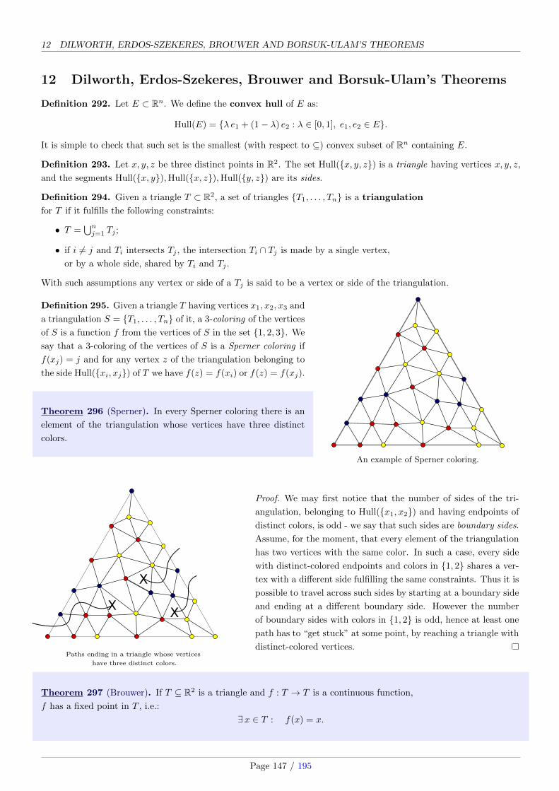
12 DILWORTH, ERDOS-SZEKERES, BROUWER AND BORSUK-ULAM’S THEOREMS
12 Dilworth, Erdos-Szekeres, Brouwer and Borsuk-Ulam’s Theorems
Definition 292. Let E ⊂ Rn. We define the convex hull of E as:
Hull(E) = {λ e1 + (1− λ) e2 : λ ∈ [0, 1], e1, e2 ∈ E}.
It is simple to check that such set is the smallest (with respect to ⊆) convex subset of Rn containing E.
Definition 293. Let x, y, z be three distinct points in R2. The set Hull({x, y, z}) is a triangle having vertices x, y, z,
and the segments Hull({x, y}),Hull({x, z}),Hull({y, z}) are its sides.
Definition 294. Given a triangle T ⊂ R2, a set of triangles {T1, . . . , Tn} is a triangulation
for T if it fulfills the following constraints:
• T =⋃nj=1 Tj ;
• if i 6= j and Ti intersects Tj , the intersection Ti ∩ Tj is made by a single vertex,
or by a whole side, shared by Ti and Tj .
With such assumptions any vertex or side of a Tj is said to be a vertex or side of the triangulation.
Definition 295. Given a triangle T having vertices x1, x2, x3 and
a triangulation S = {T1, . . . , Tn} of it, a 3-coloring of the vertices
of S is a function f from the vertices of S in the set {1, 2, 3}. We
say that a 3-coloring of the vertices of S is a Sperner coloring if
f(xj) = j and for any vertex z of the triangulation belonging to
the side Hull({xi, xj}) of T we have f(z) = f(xi) or f(z) = f(xj).
Theorem 296 (Sperner). In every Sperner coloring there is an
element of the triangulation whose vertices have three distinct
colors.
An example of Sperner coloring.
X X
X
Paths ending in a triangle whose vertices
have three distinct colors.
Proof. We may first notice that the number of sides of the tri-
angulation, belonging to Hull({x1, x2}) and having endpoints of
distinct colors, is odd - we say that such sides are boundary sides.
Assume, for the moment, that every element of the triangulation
has two vertices with the same color. In such a case, every side
with distinct-colored endpoints and colors in {1, 2} shares a ver-
tex with a different side fulfilling the same constraints. Thus it is
possible to travel across such sides by starting at a boundary side
and ending at a different boundary side. However the number
of boundary sides with colors in {1, 2} is odd, hence at least one
path has to “get stuck” at some point, by reaching a triangle with
distinct-colored vertices.
Theorem 297 (Brouwer). If T ⊆ R2 is a triangle and f : T → T is a continuous function,
f has a fixed point in T , i.e.:
∃x ∈ T : f(x) = x.
Page 147 / 195

Before starting an actual proof it is practical to introduce the concepts of trilinear coordinates
and mesh of a triangulation.
Definition 298. Given a triangle T ⊆ R2 with vertices A,B,C and a point x ∈ T , let us denote
dA(x) = d(x,BC), dB(x) = d(x,AC), dC(x) = d(x,AB),
where the distance of a point from a segment is defined as usual:
d(x,AB) = minλ∈R
d(x, λA+ (1− λ)B).
We say that the trilinear coordinates of x are given by:(dA(x)
dA(x) + dB(x) + dC(x),
dB(x)
dA(x) + dB(x) + dC(x),
dC(x)
dA(x) + dB(x) + dC(x)
).
A point belonging to T has non-negative trilinear coordinates, whose sum equals 1.
By trilinear coordinates, any continuous function from T in T can be interpreted as a continuous function from D ⊆ R3
in itself, where:
D = {(x, y, z) ∈ R3 : x, y, z ≥ 0, x+ y + z = 1}.
Definition 299. The mesh of a triangulation is the maximum side length for the elements of such triangulation.
Definition 300. Given two triangulations S and S′, we say that S′ extends or refines S if every element of S is given
by the union of some elements in S′.
Proof. Let S be a triangulation of D with mesh ε. Assuming f has no fixed points, we may give a color to every
vertex (a, b, c) in S according to (a′, b′, c′) = f((a, b, c)):
• if a′ < a, we give to (a, b, c) the color 1;
• if a′ ≥ a and b′ < b, we give to (a, b, c) the color 2;
• if a′ ≥ a and b′ ≥ b, then c′ < c, and we give to (a, b, c) the color 3.
We leave to the reader to check this coloring is a Sperner coloring. It follows there is an element Tj ∈ S whose vertices
have three distinct colors. The triangulation S can be extended to a triangulation S′ having mesh ε2 -fine: by following
the above instructions for assigning colors and repeating the same construction multiple times, we may reach the
wanted conclusion through the Bolzano-Weierstrass Theorem. In Tj there is a point t that is the common limit of
three distinct sequences of points: the first sequence made by points with color 1, the second sequence made by points
with color 2 and the third sequence made by points with color 3. However f is uniformly continuous over D, hence
for any x ∈ D there is a neighbourhood of x with at most two colors. This leads to a contradiction, proving that f
surely has a fixed point in D.
Corollary 301 (Brouwer). If D is a closed disk in R2 and f : D → D is a continuous function,
f has a fixed point in D.
Proof. Let T ∈ R2 be a triangle and let us assume the existence of a continuous and invertible map g : T → D
with a continuous inverse function. Such assumptions grant
(g−1 ◦ f ◦ g) : T → T
has a fixed point x ∈ T , from which g(x) ∈ D is a fixed point for f .
To prove the existence of the previous map g is an exercise left to the reader.
Page 148 / 195

12 DILWORTH, ERDOS-SZEKERES, BROUWER AND BORSUK-ULAM’S THEOREMS
Theorem 302 (Tucker). Let P1, . . . , P2n ∈ ∂B(0, 1) ⊆ R2 such that −Pj = Pn+j for any j ∈ [1, n]. Let S be a
triangulation of E = Hull({P1, . . . , P2n}) and f a 4-coloring of the vertices of S, with colors given by {−2,−1,+1,+2},such that:
∀j ∈ [1, n], f(Pj) = −f(Pn+j).
With such assumptions, a side of S has opposite-colored endpoints.
A Tucker coloring: red is opposite to green
and yellow is opposite to purple.
Proof. If the sides forming ∂E never have opposite-colored endpoints,
on the boundary of E there are an odd number of segments whose
endpoints have colors −1 and +2. Assuming that in S \∂E we do not
have segments with opposite-colored endpoints, every element of S
with a side colored by −1 and +2 has another side fulfilling the same
constraints: travelling across such sides by starting from the exterior
of E we get that some path necessarily stops at the interior of E.
Corollary 303. Every continuous function f : D = B(0, 1)→ R2
such that
∀x ∈ ∂D, f(x) = −f(−x)
has a zero in D.
Assuming that f is non-vanishing on D, the function g : D → S1
defined by
g(x) =f(x)− f(−x)
‖f(x)− f(−x)‖is continuous and fulfills the constraint
∀x ∈ ∂D, g(x) = −g(−x).
It follows we may give to every point of (a, b) ∈ D a color
in the set {−2,−1,+1,+2} according to (c, d) = g((a, b)):
X
X
The proofs of Sperner’s Theorem
and Tucker’s Theorem are very similar.
• if d ≥ 0 and c > 0, we give to (a, b) the color +1;
• if d > 0 and c ≤ 0, we give to (a, b) the color +2;
• if d < 0 and c ≤ 0, we give to (a, b) the color −1;
• if d ≤ 0 and c > 0, we give to (a, b) the color −2.
Considering 2n points on ∂D pairwise symmetric with respect to the origin and a triangulation with mesh ε of their
convex hull, the coloring given by the above algorithm fulfills the hypothesis of Tucker’s Theorem. It follows we have
two distinct points z, w ∈ D such that
‖z − w‖ ≤ ε, ‖g(z)− g(w)‖ ≥√
2,
Page 149 / 195

leading to a contradiction by the uniform continuity of g on D. Thus f has a fixed point in D.
Theorem 304 (Borsuk-Ulam). If f : S2 → R2 is a continuous function, there exist two antipodal points on S2
where the function f attains the same value.
Proof. Assume, by contradiction, that for any x ∈ S2 = ∂B(0, 1) ⊆ R3 we have
f(x) 6= f(−x). There exists a continuous and invertible function g from S2 ∩ {z ≥ 0}in D2 = {(x, y) ∈ R2 : x2 + y2 ≤ 1}, which coincides with the identity function when restricted to S1 = S2 ∩ {z = 0}:
g((x, y,
√1− (x2 + y2)
))= (x, y).
As a consequence, there exists h : D2 → R2, defined by:
h(x) = f(g−1(x))− f(−g−1(x)),
which is continuous, non-vanishing and fulfilling h(x) = −h(−x) on the points of ∂D2 = S1.
However, such a function cannot exist by the previous result.
Corollary 305. At every moment, there exist two antipodal points on the surface of Earth
having the same temperature and the same pressure.
Theorem 306 (Lusternik-Schnirelmann). If C1, C2, C3 are three closed sets covering S2,
at least one of them contains a couple of antipodal points.
Proof. Since the functions di : S2 → R, with i ∈ {1, 2, 3}, defined by:
di(x) = miny∈Ci
‖x− y‖
are continuous, the function f : S2 → R2 definined by:
f(x) = (d1(x), d2(x))
is continuous as well. Due to Borsuk-Ulam’s Theorem there exists some x ∈ S2 such that:
(d1(x), d2(x)) = f(x) = y = f(−x) = (d1(−x), d2(−x)) .
If y has its first or second component equal to zero, then both x and −x belong to C1 or C2, respectively. If y does
not have any component equal to zero, then neither x or −x belong to C1 or C2, hence they necessarily belong to C3,
since:
S2 =
3⋃i=1
Ci.
Exercise 307. Prove that Lusternik-Schnirelmann’s Theorem is equivalent to Borsuk-Ulam’s Theorem.
Surprisingly, these quite deep results in Topology have interesting applications in Combinatorics. If we denote by
[n] the set {1, 2, . . . , n} and by(
[n]k
)the subsets of [n] with k elements, the Kneser graph KG(n, k) is the graph
admitting(
[n]k
)as vertex set and having edges only between nodes associated with disjoint subsets. Given a finite,
undirected graph G, its chromatic number χ(G) is defined as the minimum number of colors required to give a
color to every vertex of G, in such a way that neighbours have distinct colors.
Page 150 / 195

12 DILWORTH, ERDOS-SZEKERES, BROUWER AND BORSUK-ULAM’S THEOREMS
Theorem 308 (Kneser’s Conjecture / Lovasz Theorem).
χ(KG(n, k)) = n− 2k + 2.
It is not difficult to prove that χ(KG(n, k)) ≤ n− 2k + 2, for instance by giving to any vertex v ∈ V associated with
a subset F the color defined by min (F ∪ {n− 2k + 2}). With such assumptions, if F1 and F2 have the same color
i < (n− 2k+ 2), then i ∈ F1 ∩ F2, hence (F1, F2) ∈ E. On the other hand, if both F1 and F2 have color (n− 2k+ 2),
both of them are subsets of {n−2k+2, n−2k+2, . . . , n}, which is a set with cardinality 2k−1. As a consequence, F1
and F2 have a non-empty intersection. Laszlo Lovasz proved Kneser’s conjecture in 1978 by using the Borsuk-Ulam
theorem, and his proof has been greatly simplified in 2002 by J. Greene (just a college student at the time). Le us
set d = n− 2k + 1: we wish to prove that χ(KG(n, k)) > d. Let X ⊆ Sd be a set of n points in general position (i.e.
such that at most d points of X belong to a hyperplane through the origin) and let us consider X and [n] as the same
object. Assuming to have a valid (in the chromatic number sense) coloring of KG(n, k) using d colors, let us define,
for any x ∈ Sd, H(x) as the open hemisphere made by points y such that 〈x, y〉 > 0. Additionally, let us define a
covering A1, A2, . . . , Ad+1 of Sd as follows: for any i = 1, 2, . . . , d we let
Aidef=
{x : ∃F ∈
(X
k
)with color i such that F ⊆ H(x)
}and define Ad+1 as Sd \
⋃di=1Ai. Invoking the Lusternik-Schnirelmann Theorem, there exists some x ∈ Sd such that
both x and −x belong to Ai for some i ∈ [d + 1]. If i ≤ d, H(x) and H(−x) contain, respectively, sets F1 and F2 of
the same color, i, but since H(x) and H(−x) are disjoint, F1 and F2 are disjoint, hence they cannot have the same
color, since there is an edge between them. If i = d + 1, then both x and −x belong to Ad+1, hence H(x) contains
at most (k − 1) points from X (otherwise H(x) would contain some F with color j ≤ d and x would belong to Aj
and not to Ad+1). In a similar way, H(−x) contains at most (k − 1) points from X, hence Sd \ (H(x) ∪H(−x)), a
subset of the hyperplane 〈x, y〉 = 0, contains at least n− 2k+ 2 = d+ 1 punti, which contradicts the previous “general
position” assupmtion. We may notice that in order to plane n points on Sn in general position it is enough to follow a
probabilistic approach: a random configuration (with respect to the uniform probability distribution on Sn) is almost
surely in general position. A deterministic approach is to exploit the moment curve t→ (1, t, . . . , td): it is simple to
prove by Ruffini’s rule that d distinct points on the curve, together with the origin, never lie on the same hyperplane.
By normalizing these d points one gets d points in general position on Sd−1.
Corollary 309. There are triangle-free graphs with an arbitrarily large chromatic number.
This results is usually proved by invoking Mycielski’s construction: let G = ([n], E) be a triangle-free graph and let
us consider the graph having vertex set {1, 2, . . . , 2n, 2n+ 1} and the following set of edges:
• an edge between j and k if (j, k) is an edge in G;
• an edge between n+ τ and k if (τ, k) is an edge in G;
• an edge between 2n+ 1 and n+ τ for any τ ∈ [n].
This is a triangle-free graph and its chromatic number equals χ(G) + 1.
Kneser graphs provide an alternative construction: if n < 3k, KG(n, k) is triangle-free, hence
KG(3M − 4,M − 1)
for any M ≥ 3, is a triangle-free graph with chromatic number M by Lovasz’ Theorem.
Kneser graphs play a crucial role in another remarkable result:
Page 151 / 195

Theorem 310 (Erdos-Ko-Rado). If A is a family of subsets with cardinality r of {1, 2, . . . , n}, with n ≥ 2r,
and every couple of elements of A has a non empty intersection, then:
|A| ≤(n− 1
r − 1
).
In terms of Kneser graphs, the Erdos-Ko-Rado Theorem states that(n−1r−1
)= α(KG(n, k)) is the maximum number of
elements in a independent subset of KG(n, k), i.e. a subset of the vertex set in which there are no edges from the
original graph. The proof we are going to outile is due to Katona (1972). Let us assume to arrange the elements of
{1, 2, . . . , n} in a cyclic ordering, and to consider the intervals with length r in this ordering. For instance, assuming
n = 8 and r = 3, the cyclic ordering (3, 1, 5, 4, 2, 7, 6, 8) produces the intervals:
(3, 1, 5), (1, 5, 4), (5, 4, 2), (4, 2, 7), (2, 7, 6), (7, 6, 8), (6, 8, 3), (8, 3, 1).
However it is not possible that all these intervals belong to A, since many of them are disjoint. The key observation
of Katona is that at most r of these intervals may belong to A, disregarding the considered cyclic ordering. Indeed,
if (a1, a2, . . . , ar) is an interval belonging to A, any other interval of the same cyclic ordering belonging to A has to
separate ai and ai+1 for some i, i.e. it has to contain exactly one of these two elements. The two intervals separating
these two elements are disjoint, hence at most one of them may belong to A. As a consequence, the number of intervals
belonging to A is at most 1 plus the number of “separable couples”, i.e. ≤ 1 + (r − 1) = r. Now we may count the
number of couples (S,C) where S is a set in A and C is a cyclic ordering for which S is an interval. On one hand,
for any S it is possible to generate C by choosing the r! permutations of S and the (n − r)! permutations of the
remaining elements. In particular the number of the previous (S,C) couples is |A|r!(n− r)!. On the other hand, there
are (n − 1)! cyclic orderings, and any of them produces at most r intervals belonging to A, hence the number of the
previous (S,C) couples is at most r(n− 1)!. By double counting :
|A|r!(n− r)! ≤ r(n− 1)! ←→ |A| ≤(n− 1
r − 1
).
Theorem 311 (Lubell-Yamamoto-Meshalkin). Let A be a family of subsets of {1, 2, . . . , n}, with the property that
two distinct elements A1, A2 ∈ A never fulfill A1 ⊆ A2 or A2 ⊆ A1. By denoting as τk the number of elements in Awith cardinality k, we have:
n∑k=0
τk(nk
) ≤ 1.
The proof of this remarkable result is very similar to the outlined proof of the Erdos-Ko-Rado Theorem. A family
of subsets fulfilling the hypothesis is also said to be a Sperner family, and it is an antichain in the partial ordering
of the subsets of {1, 2, . . . , n} induced by ⊆. If we consider a random ordering (x1, x2, . . . , xn) of [n] and the sets
C0 = ∅, . . . , Ck = {x1, . . . , xk}, every couple of elements of C = {C0, C1, . . . , Cn} fulfills ⊆ or ⊇, hence the expected
value of |C ∩ A| certainly is ≤ 1. On the other hand, for any A ∈ A the probability that A belongs to the random
chain C is exactly(n|A|)−1
, since C contains just one set with cardinality |A|, and the probability is uniform over any
element of A. In particular:
1 ≥ E[|A ∩ C|] =∑A∈A
P[A ∈ C] =∑A∈A
1(n|A|) =
n∑k=0
τk(nk
) .
Page 152 / 195
12 DILWORTH, ERDOS-SZEKERES, BROUWER AND BORSUK-ULAM’S THEOREMS
Corollary 312 (Sperner). Given the set {1, 2, . . . , n}, the Sperner family with the greatest number of elements
is the one made by the sets with cardinality bn/2c.
Hall’s Theorem is also known as Hall’s marriage Theorem, since it is usually presented through this formulation 10:
let us suppose to have n women and n men, and that every woman has her personal set of potential partners among
the previous n men. Which conditions ensure it is possible to declare them all wife and husband, without marrying
any woman with someone not in her list of candidates? Hall’s Theorem states that necessary and sufficient conditions
are provided by having no subset of women with a joint list of candidates that is too small.
Definition 313. We say that a graph G = (V,E) admits a perfect matching if there exists E′ ⊆ E such that the
elements of E′ do not have any common vertex and every vertex v ∈ V is an endpoint for some edge in E′.
Theorem 314 (Hall’s marriage Theorem, 1935). Let us assume that G = (V,E) is a balanced bipartite graph, i.e.
V = F ∪M , F ∩M = ∅, |F | = |M | and every edge in G joins a vertex in F with a vertex in M . G has a perfect
matching if and only if for any non-empty subset F ′ ⊆ F , the number of neighbours of F ′ in M is ≥ |F ′|.
Proof. Part of the claim is trivial: if a perfect matching exists, clearly every non-empty subset F ′ ⊂ F has a neigh-
bourhood in M whose cardinality is ≥ |F ′|.The converse implication is not trivial, but it is a consequence of Dilworth’s Theorem. We are going to approach the
proof of Hall’s Theorem through a maximality argument. Let us assume |F | = |M | = n and that the hypothesis of
Hall’s Theorem are fulfilled, but no perfect matching exists. We may consider C ⊆ E that is a coupling, i.e. a set of
disjoint edges, with the maximum cardinality, then denote through FC , FE\C , respectively, the sets of elements of F
reached / not reached by C. In a similar way we may define MC and ME\C . We may notice that every element of E
has an endpoint in C, otherwise C would not be maximal. There are at least |FE\C | edges of G with an endpoint in
FE\C , and for all of them the other enpoint has to lie in MC , again by maximality of C. In particular |MC | ≥ |FE\C |which implies |MC | = |FC | ≥ n
2 . On the other hand, all the edges of C with an endpoint in FC have the other endpoint
in MC . In order that F fulfills the given hypothesis, there have to be at least |ME\C | edges of G joining FC and ME\C .
If f ∈ FC and m ∈MC are joined by an edge in C and, additionally, f is joined with an element of ME\C by e1 ∈ Eand m is joined with an element of FE\C by e2 ∈ E, by removing from C the edge (m, f) and inserting the edges e1, e2
we get a coupling with a greater cardinality, violating the maximality of C. Since that cannot happen, we may define
M ′C as the neighbourhood of FE\C in MC and consider that C induces a bijection between M ′C and a subset of FC .
Let us denote such subset as F ′C . If FE\C is non-empty and FE\C ∪ F ′C meets the hypothesis, the neighbourhood of
F ′C in MC contains at least one element not belonging to M ′C . If we denote as M ′′C the last neighbourhood and repeat
the same construction, we ultimately get that there are no edges of E between FC and ME\C , but in such a case F
does not meet the hypothesis. It follows that FE\C is empty and C is a perfect matching.
10Truth to be told, the very usual formulation has the roles of women and men exchanged. It does not really matter... or does it?
Page 153 / 195

A summary of the key steps in the proof of Hall’s Theorem.
The elements of C are blue, the elements of E \ C are black.
• (I) : C induces a bijection between FC and MC , but there have to be some edge of E
joining FE\C and MC , together with some edge of E joining ME\C and FC ;
• (II) : the depicted situation cannot happen, since otherwise we could remove an edge from C
and insert two edges, getting a larger coupling;
• (III) : on the other hand the neighbourhood of the red points cannot be made by purple points only,
since otherwise the set of red points would violate the hypothesis.
Exercise 315. Exploiting Hall’s Theorem, prove that if we remove two opposite-colored squares from a 2n × 2n
chessboard, the remaining part can be tiled by dominoes like or its 90◦-rotated version.
Exercise 316 (Birkhoff). We say that a n × n matrix is doubly stochastic if its entries are non-negative and the
sum of the entries along every row or column equals one. Prove that any doubly stochastic matrix can be written as
a convex combination of permutation matrices.
Theorem 317 (Erdos-Szekeres). From each sequence of mn + 1 real numbers it is possible to extract a weakly
increasing subsequence with n+ 1 terms, or a weakly decreasing subsequence with m+ 1 terms.
Proof. The proof we are going to outline proceeds in a algorithmic fashion: let us assume that a1, a2, . . . , amn+1 is the
main sequence and that we have n queues in a post office, initially empty, where to insert the elements of the main
sequence one by one. For any i ∈ {1, . . . , } we act as follows: ai visits the first queue and if it is empty, or the value
of ai is greater than the value of the last entry of the queue, ai takes place in such a queue, otherwise it goes to the
next queue and behaves in the same way. If, at some point, some element a of the original sequence is not able to
take place in any queue, the subsequence given by the last entries of each queue, together with a, provides a weakly
decreasing subsequence with n + 1 terms. Conversely, if every element of the original sequence is able to take place
Page 154 / 195
12 DILWORTH, ERDOS-SZEKERES, BROUWER AND BORSUK-ULAM’S THEOREMS
somewhere, at the end of the process there will be mn + 1 entries in n queues, hence at least a queue with m + 1
entries by the Dirichlet box principle, with such queue providing an increasing subsequence with m+ 1 terms.
The Erdos-Szekeres Theorem can be exploited to outline a “quantitative” proof of the Bolzano-Weierstrass Theorem.
If {an}n≥1 is a sequence of real numbers belonging to the interval [a, b], the Erdos-Szekeres Theorem allows us to
extract a weakly monotonic subsequence. Since every bounded and weakly monotonic sequence is convergent to its
infimum or supremum, every bounded sequence has a convergent subsequence.
The Erdos-Szekeres Theorem has been the key for proving the following statement, too:
Theorem 318 (Happy Ending Problem11). Given some positive integer N , in every set of distinct points in R2
with a sufficiently large cardinality there are the vertices of a convex N -agon.
By denoting as f(N) the minimum cardinality granting the existence of a convex N -agon, up to 2015 the sharpest
bound for f(N) was
∀N ≥ 7, f(N) ≤(
2N − 5
N − 2
)+ 1 = O
(4N√N
),
but in 2016 Suk and Tardos presented an article (currently under revision) where they claimed f(N) = 2N+O(√N logN),
i.e. an almost-optimal bound, since it is not difficult to prove that f(N) ≥ 1 + 2N−2. The Erdos-Szekeres can also be
exploited to prove the following statement (even if “the usual way” is to do just the opposite):
Theorem 319 (Dilworth-Mirsky). Given a partial ordering on a finite set, the maximum length of a chain equals the
minimum number of chains in which the original set can be partitioned.
The last part of this section is dedicated to a famous application of the combinatorial compactness principle:
in some cases it is possible to prove statements for finite sets by deducing them from statements involving infinite sets.
Theorem 320 (Ramsey, 1930). For any n ≥ 1 there exists an integer R(n) such that,
given any 2-coloring of the edges of KR(n), there exists a monochromatic subgraph Kn.
We are going to prove such claim by starting with its infinite version:
Theorem 321 (Ramsey, infinite version). Let k, c ≥ 1 be integers, and let V be an infinite set.
Given any coloring of(Vk
)with c colors, there exists an infinite subset U ⊆ V such that
(Uk
)is monochromatic.
Proof. We proceed by induction on k: if k = 1 the claim is trivial.
So we may assume that k ≥ 2 and(Vk
)is colored through c colors, i.e. there exists a map χ :
(Vk
)→ C where |C| = c.
We wish to construct an infinite sequence V0 ⊃ V1 ⊃ V2 ⊃ . . . of infinite subsets of V , together with an infinite
sequence of elements x0, x1, x2, . . . such that, for any i:
• (I) xi ∈ Vi and Vi+1 ⊆ Vi \ {xi};
• (II) the k-subsets of the form {xi} ∪ Y , as Y ranges over Vi+1, all have the same color c(i).
11Erdos gave such a name to this problem since it someway contributed to making George Szekeres and Esther Klein a married couple.
Page 155 / 195

We start by setting V0 = V and we pick some x0 ∈ V . Let us assume to already have V0, V1, . . . , Vi and x0, x1, . . . , xi.
We want to construct a couple (Vi+1, xi+1): for such a purpose we introduce an auxiliary coloring χi, which assigns
to any Y ∈(Vi\{xi}k−1
)the color of the k-subset {xi} ∪ Y in the original coloring χ, i.e.:
χi :
(Vi \ {xi}k − 1
)→ C
Y → χ({xi} ∪ Y ).
This construction produces a c-coloring χi of(Vi\{xi}k−1
). Since Vi \ {xi} is infinite, the inductive hypothesis ensures
the existence of an infinite subset Vi+1 which is (k− 1)-monochromatic. Additionally we get that, with respect to the
original coloring χ, all the k-subsets of Vi+1 ∪ {xi} containing the element xi have the same color, which we denote
as c(i). Let xi+1 be any element of Vi+1. The sequences produced by our algorithm clearly fulfill (I) and (II). Since
c is finite, the Dirichlet box principle ensures the existence of an infinite subset A ⊂ N such that for any i ∈ A the
color c(i) is always the same. By letting U = {xi : i ∈ A} we get an infinite subset of V that is k-monochromatic as
wanted.
If we restrict our attention to graphs (i.e. to the k = 2 case), the Theorem just proved can be also stated in the
following way: let G be a graph with an infinite vertex set V , such that for any infinite subset X ⊂ V there is an
edge of V whose endpoints belong to X. Then G contains an infinite complete subgraph. In order to prove the finite
version, it is enough to invoke the following Lemma, which can be informally stated as in a infinite tree there is an
infinite branch.
Lemma 322 (Konig’s infinity Lemma). Let G = (V,E) a graph with an infinite vertex set. Let V =⋃i≥0 Vi, where
V0, V1, . . . are finite, non-empty and disjoint sets. Let us assume there is a map f : V \V0 → V such that for any v ∈ Viwith i ≥ 1, f(v) ∈ Vi−1 and {v, f(v)} ∈ E. Then there exists an infinite sequence v0, v1, v2, . . . such that vi ∈ Vi and
vi = f(vi+1) for any i ≥ 0.
Proof. Let us denote through C the set of “f -paths”, i.e. the set of paths of the form
v, f(v), f2(v), . . . , fs(v)(v),
terminating at some element fs(v)(v) ∈ V0. Any v ∈ V is a vertex for an element of C and every f -path is finite, hence
C has to contain an infinite number of paths. Since V0 is a finite set, there exists an infinite subset C0 ⊆ C made by
paths terminating at some v0 ∈ V0. Since V1 is a finite set, there exists at least one vertex v1 ∈ V1 such that the subset
C1 ⊆ C0, made by paths through v1, is infinite. By repeating the same argument we easily get an infinite sequence
v0, v1, . . . meeting the wanted constraints.
We are ready to deduce the finite version of Ramsey’s Theorem from its infinite version.
For any r ∈ N+, let us denote as Ir the set {1, 2, . . . , r}. Let us assume the existence of a triple (k, c, n) such that,
for any integer r ≥ k, there exists a c-coloring γr :(Irk
)→ |C|, with |C| = c, of the k-subsets of Ir, such that no
n-subset of Ir is k-monochromatic (i.e. for any X ⊆ Ir with cardinality n, there exist Y and Y ′ in(Xk
)such that
γr(Y ) 6= γr(Y′)).
Denoting through Vr the set of this “faulty” c-colorings γr of Ir, every Vr is finite and non-empty. Let us set
V =⋃r≥k Vr. For r ≥ k and γ ∈ Vr+1, let us define f(γ) as the restriction of γ to Ir. f(γ) then is an element of Vr
(the restriction of a faulty coloring still is a faulty coloring). By considering G = (V,E), where the edge set is given by
E = {{γ, f(γ)} : γ ∈ V \Vk}, we are in the hypothesis of Konig’s infinity Lemma. It follows the existence of a coloring of(Nk
)which is faulty when restricted to any Ir. This contradicts the statement of Ramsey’s theorem in its infinite version.
Page 156 / 195

12 DILWORTH, ERDOS-SZEKERES, BROUWER AND BORSUK-ULAM’S THEOREMS
Some remarkable results in Infinite Combinatorics.
Theorem 323 (Schur). For any coloring of N with a finite number of colors,
there exist infinite triples of the form (a, b, a+ b) which are monochromatic.
Theorem 324 (Van Der Waerden). For any coloring of N with a finite number of colors,
there exist monochromatic arithmetic progressions of arbitrary length.
Theorem 325 (Hales-Jewett). For any coloring of Zd with a finite number of colors, there exist infinite monochro-
matic sets of the form P1 × P2 × . . .× Pd, in which every Pk is an arithmetic progression in Z.
Theorem 326 (Szemeredi). The claim of Van Der Waerden’s Theorem still holds if N is replaced by a subset of
N with positive asymptotic density.
Theorem 327 (Green-Tao). The set of prime numbers contains arithmetic progressions with arbitrary length.
Exercise 328. Let us consider a graph G having N as its vertex set and edges joining a and b iff |a− b|is a number of the form m! for some m ∈ N+. Prove that the chromatic number of G equals 4.
Exercise 329 (Sarkozy). Let us consider a graph G having N as its vertex set and edges joining a and b iff |a− b|is a number of the form m2 for some m ∈ N+. Prove that the chromatic number of G is +∞. Hint: use a refined
version of Van Der Corput’s trick to show that in any subset of N with positive asymptotic density, there are two
distinct elements whose difference is a square.
Page 157 / 195

13 Continued fractions and elements of Diophantine Approximation
A (ordinary) continued fraction is an object of the following form 12:
a0 +1
a1 + 1a2+...
,
where a0 is a non-negative integer and every aj with j ≥ 1 is a positive integer.
For the sake of brevity and readability, the following compact notations are used very often:
[a0; a1, a2, . . . , an] or a0 +1
a0+
1
a0+. . .
1
an.
The numbers aj are said terms or partial quotients of the continued fraction, while the following rational numbers
q0 = a0, q1 = [a0; a1], q2 = [a0; a1, a2], . . .
are said convergents of the continued fraction. We may notice that:
[a0; a1, . . . , an, 1] = [a0; a1, . . . , an + 1],
hence from now on we will assume that the last term of a ordinary continued fraction (associated with an element of
Q+ \ N) is never 1, in order to preserve the unicity of the representation.
Theorem 330. Every rational number q ∈ Q+ has a unique continued fraction representation.
We may simply consider the orbit of q with respect to the map ϕ : x 7→ 1x−bxc .
For instance, by starting at q = 247 we have:
24
7= 3 +
3
7,
7
3= 2 +
1
3,
from which:24
7= 3 +
1
2 + 13
= [3; 2, 3].
We may notice that the fractional parts involved in the process are rational numbers < 1 and their numerators form
a strictly decreasing sequence: if at some point we are dealing with a fractional part ab with a < b, at the next step
the numerator of the new fractional part is b −⌊ba
⌋a < a. It follows that at some point the involved fractional part
has a unit numerator and the previous algorithm stops, producing a continued fraction representation for q.
Lemma 331. If two continued fractions with n+ 1 terms [a0; a1, . . . , an] = qa and [b0; b1, . . . , bn] = qb
share the first n terms and an > bn, then qa > qb or qa < qb according to the parity of n.
The result can be simply proved by induction on n: the base case n = 0 is trivial and the inequality
[c0; c1, . . . , cn−1, c] < [c0; c1, . . . , cn−1, d]
is equivalent, up to substracting c0 from both terms, to the inequality:
[0; c1, . . . , cn−1, c] < [0; c1, . . . , cn−1, d],
or, by considering the reciprocal of both the RHS and the LHS, to the inequality:
[c1; . . . , cn−1, c] > [c1; . . . , cn−1, d],
12Temporarily, we will assume to deal with a finite number of nested ratios. We will see soon that this assumption can be dropped, and
dropping such assumption leads to an algorithmic way for representing every element of R+ as a continued fraction.
Page 158 / 195

13 CONTINUED FRACTIONS AND ELEMENTS OF DIOPHANTINE APPROXIMATION
whose truth follows from the inductive hypothesis. In general, two continued fractions which differ by at least one
term represent two distinct rational numbers. Let us assume to have:
[a0; a1, . . . , an, b0, . . . , bm] = [a0; a1, . . . , an, c0, . . . , cr],
with b0 6= c0. By subtracting a suitable integer number from both sides and reciprocating n+ 1 times we get:
[b0; . . . , bm] = [c0; . . . , cr]
which leads to a contradiction, since by applying x 7→ bxc to both sides of the last supposed identity we get two distinct
integer numbers. This proves that any positive rational number can be represented in a unique way as a continued
fraction. We may also notice that the process leading to the construction of the terms of the continued fraction of ab ,
where a and b are coprime positive integers, is analogous to the application of the extended Euclidean algorithm for
computing gcd(a, b). Since a and b are coprime by assumption, gcd(a, b) = 1 and the Euclidean algorithm stops in a
finite number of steps, producing a finite continued fraction representing ab .
Theorem 332. Let hm and km, respectively, the numerator and denominator of the m-th convergent of the continued
fraction [a0; a1, . . . , an]. For any integer x ≥ 1 we have:
[a0; a1, . . . , an, x] =xhn + hn−1
x kn + kn−1.
Proof. We may prove the statement by induction on n: the base case n = 2 is simple to check. Let pm and qm be the
numerator and denominator of the m-th convergent of [a1; . . . , an, x]. We have:
[a0; a1, . . . , an, x] = a0 +qnpn
=a0pn + qn
pn,
but the inductive hypothesis ensures pn = x · pn−1 + pn−2 and qn = x · qn−1 + qn−2, from which:
[a0; a1, . . . , an, x] =x(a0pn−1 + qn−1) + (a0pn−2 + qn−2)
xkn + kn−1=xhn + hn−1
x kn + kn−1.
Theorem 333. If hmkm
and hm+1
km+1are consecutive convergents of the same continued fraction,
hm+1 km − hm km+1 = (−1)m.
Proof. Let Am = hm+1 km − hm km+1. By the previous Theorem,
hm+1 = amhm + hm−1, km+1 = amkm + km−1,
from which A(m) = −A(m− 1) immediately follows.
In particular, continued fraction can be exploited for computing the multiplicative inverse of any a ∈ F∗p:
Exercise 334. Compute the inverse of 35 modulus 113 through continued fractions.
Page 159 / 195

Proof. We have that:113
35= [3; 4, 2, 1, 2], [3; 4, 2, 1] =
42
13
hence the absolute value of the difference between 11335 and 42
13 equals 135·13 . In particular:
113 · 13− 42 · 35 = −1,
hence the inverse of 35 in Z/(113Z)∗ is 42.
Corollary 335. If the continued fraction of q ∈ Q+ has n terms, by denoting as km the denominator of the m-th
convergent we have:
q = a0 −n∑j=1
(−1)j
kj−1kj.
Proof. Due to the previous Theorem we have:
q =hnkn
= a0 +
n∑j=1
(hjkj− hj−1
kj−1
)= a0 +
n∑j=1
A(j − 1)
kj−1kj.
Corollary 336. If the continued fraction of q ∈ Q+ has at least k + 2 terms and pkqk
is its k-th convergent, we have:
1
qk(qk + qk+1)≤∣∣∣∣q − pk
qk
∣∣∣∣ < 1
qk qk+1.
Proof. As a consequence of the Corollary (335) q certainly is between pkqk
and pk+1
qk+1, hence:∣∣∣∣q − pk
qk
∣∣∣∣ < ∣∣∣∣pk+1
qk+1− pkqk
∣∣∣∣ =1
qk+1qk,
where the last identity follows from the Theorem (333). On the other hand, if a, b, c, d are four positive integers,
the ratio a+cb+d certainly is between a
b and cd , hence the sequence
pkqk,pk + pk+1
qk + qk+1,pk + 2pk+1
qk + 2qk+1, . . . ,
pk + ak pk+1
qk + ak qk+1=pk+2
qk+2
is monotonic. Additionally, pkqk
and pk+2
qk+2lie on the same side with respect to q, hence:∣∣∣∣q − pkqk
∣∣∣∣ ≥ ∣∣∣∣pk + pk+1
qk + qk+1− pkqk
∣∣∣∣ =1
qk(qk + qk+1),
where the last identity is again a consequence of the Theorem (333).
Corollary 337. If the continued fraction of α ∈ Q+ has at least n+ 2 terms and pkqk
is its k-th convergent, we have:
|qkα− pk| > |qk+1α− pk+1| .
Proof. The following inequality holds as a consequence of the Corollary (336):
|qkα− pk| ≥1
qk + qk+1≥ 1
qk+2> |qk+1α− pk+1| .
Page 160 / 195

13 CONTINUED FRACTIONS AND ELEMENTS OF DIOPHANTINE APPROXIMATION
Remark. Continued fractions provide a bijection between [1,+∞) and the set of (finite or infinite) sequences of
positive integers. This leads to a very short proof of the non-countability of R:
|R| ≥ |[1,+∞)| ≥∣∣NN∣∣ ≥ ∣∣2N∣∣>|N|.
Despite not being very common, to use continued fractions to define the set of real numbers is a perfectly viable
alternative approach to using Dedekind cuts or the completion of a metric space, since continued fractions encode the
order structure of R in a very efficient way.
Theorem 338 (Hurwitz). If we consider two consecutive convergents of the continued fraction of α ∈ (R \Q)+,
at least one of them fulfills: ∣∣∣∣α− p
q
∣∣∣∣ ≤ 1
2 q2.
Proof. Let us assume, by contradiction, that both pkqk
and pk+1
qk+1violate the previous inequality.
Such assumptions lead to:
1
qkqk+1=
∣∣∣∣pkqk − pk+1
qk+1
∣∣∣∣ =
∣∣∣∣α− pkqk
∣∣∣∣+
∣∣∣∣α− pk+1
qk+1
∣∣∣∣ ≥ 1
2q2k
+1
2q2k+1
,
from which:
2qkqk+1 ≥ q2k + q2
k+1,
or 0 ≥ (qk+1 − qk)2, implying k = 0 and qk = 1: in such a case, however,∣∣∣α− p0
q0
∣∣∣ < 12 .
Theorem 339 (Hurwitz). If we consider three consecutive convergent of the continued fraction of α ∈ (R \Q)+,
at least one of them fulfills: ∣∣∣∣α− p
q
∣∣∣∣ ≤ 1√5 q2
.
Proof. Let us assume that the consecutive convergents pkqk, pk+1
qk+1, pk+2
qk+2all violate the wanted inequality. In such a case:
1
qkqk+1>
1√5q2k
+1√
5q2k+1
,1
qk+1qk+2>
1√5q2k+1
+1√
5q2k+2
,
hence by setting λ1 = qk+1
qkand λ2 = qk+2
qk+1we have:
λ2i −√
5λi + 1 < 0,
from which it follows that λi ∈(√
5−12 ,
√5+12
). This leads to:
λ2 =qk+2
qk+1= ak+1 +
1
λ1> 1 +
2√5 + 1
=
√5 + 1
2,
i.e. to a contradiction.
Theorem 340 (Hurwitz duplication formula).
2 [0, 2a+ 1, b, c, . . .] = [0, a, 1, 1 + 2 [0, b− 1, c, . . .]] ,
2 [0, 2a, b, c, . . .] = [0, a, 2 [b, c, . . .]] .
Page 161 / 195

Proof. Let x = [b, c, . . .]. In such a case the LHS of the first equality is given by
2 · 1
(2a+ 1) + 1x
=2x
(2a+ 1)x+ 1
and the RHS of the first equality is given by
1
a+ 11+ 1
1+ 2x−1
=1
a+ 11+ x−1
x+1
=1
a+ x+12x
=2x
2ax+ (x+ 1).
Similarly, in order to prove the second equality it is enough to check that:
2 · 1
2a+ 1x
=1
a+ 12x
.
Hurwitz duplication formula leads to a simple derivation of the continued fraction of e, related with the interplay
between continued fractions and Riccati differential equations. Let f0(x) = tanh(x) and
fn+1(x) =1
fn(x)− 2n+ 1
x.
The Taylor series of f0(x) at the origin is x − x3
3 + . . ., so 1f0(x) has a simple pole with residue 1 at the origin and
f1(x) = 1f0(x) −
1x is an analytic function in a neighbourhood of the origin. It is not difficult to prove by induction that
fn(x) fulfills the differential equation f ′n(x) = 1− fn(x)2 − 2nx fn(x) and it is an analytic function in a neighbourhood
of the origin. Assuming the fact that fn(x) is uniformly bounded over n, the continued fraction representation
tanh(x) =[0, 1
x ,3x ,
5x ,
7x , . . .
](due to Lambert) follows, and a careful study reveals it is convergent over the whole C∗.By evaluating both sides of the last identity at x = 1
2 we get
e− 1
e+ 1= [0; 2, 6, 10, 14, . . .]
e+ 1
e− 1= [2; 6, 10, 14, 18, . . .]
2
e− 1= [1; 6, 10, 14, 18, . . .]
e− 1
2= [0; 1, 6, 10, 14, . . .]
e = 1 + 2 · [0; 1, 6, 10, 14, . . .]
and the continued fraction for e can be deduced from Hurwitz duplication formula.
Exercise 341. By exploiting Lambert’s continued fraction prove that for any n ∈ Z \ {0} we have en 6∈ Q,
then show that for any q ∈ Q+ \ 1 we have log q 6∈ Q.
Theorem 342 (Lagrange). If α is an irrational positive numbers and two coprime integers p, q fulfill:∣∣∣∣α− p
q
∣∣∣∣ ≤ 1
2q2,
then pq is a convergent of the continued fraction of α.
Page 162 / 195

13 CONTINUED FRACTIONS AND ELEMENTS OF DIOPHANTINE APPROXIMATION
Proof. Let [a0; a1, . . . , an] be the continued fraction of pq : such assumption grants p = pn and q = qn. By setting
β =pn−1 − αqn−1
αqn − pn
we have:
α =βpn + pn−1
βqn + qn−1, (1)
and additionally: ∣∣∣∣α− p
q
∣∣∣∣ =1
qn(βqn + qn−1).
The RHS is ≤ 12q2n
, from which:
β ≥ 2− qn−1
qn> 1.
If we represent β = [an+1; . . .] and exploit the equation (1) we have that the continued fraction of α is given by the
concatenation of the continued fraction of pq and the continued fraction of β, i.e.:
α = [a0; a1, . . . , an, an+1, . . .],
which proves that pq is a convergent of α.
Lagrange’s Theorem implies that the convergents of a continued fraction are in some sense the best rational approx-
imations for the represented positive real number. Such remark leads to an interesting approach for proving the
irrationality of some positive real numbers:
Corollary 343. If α ∈ R+ and there exists a sequence{pnqn
}n≥1
of rational numbers fulfilling
∀n ≥ 1, |qnα− pn| ≤1
2qn,
then α ∈ R \Q.
Informally speaking, if a real number is (in the previous sense) too close to the set of rational numbers, then it is
certainly irrational (kind of counterintuitive, isn’t it? ). A possible proof of the irrationality of some constant is so given
by finding an infinite number of good enough rational approximations. Remarkably, in many cases such sequences of
accurate approximations can be found by exploiting peculariar integrals and/or orthogonal polynomials: this idea can
be traced back to Beuker (≈ 1970) and it has been studied and extended by many others, like Hadjicostas, Rivoal,
Sorokin, Hata, Viola, Rhin, Nesterenko and Zudilin. Let us see a famous instance of such technique:
Lemma 344. The following approximations are pretty accurate:
e ≈ 19
7, π ≈ 22
7.
Proof. On the interval (0, 1), the positive x(1− x) is positive and never exceeds 14 .
In particular, the following integrals∫ 1
0
x2(1− x)2e−x dx = 14e− 38,
∫ 1
0
x4(1− x)4
1 + x2dx =
22
7− π
are positive but respectively bounded by 116 and 1
256 . In a similar way, π2 ≈ 49350 follows from:
1
120≥∫ 1
0
x4(1− x)2
1 + x(− log x) dx =
493
150− π2
3.
Page 163 / 195

Even better approximations can be obtained by replacing the weigths xα(1− x)β with shifted Legendre polynomials.
For instance: ∫ 1
0
P4(2x− 1)e−x dx = 1001− 2721
e≈ 4 · 10−5.
In the last case the magnitude of the involved integral is a bit more difficult to estimate, but that can be done through
Rodrigues’ formula, for instance.
Quadratic surds also play an important role in the theory of continued fractions. We wish to investigate the structure
of the continued fraction of√D, where D ∈ N+ is not a square. Let us consider, for instance, the D = 19 case:
√19 = [4; 2, 1, 3, 1, 2, 8, 2, 1, 3, 1, 2, 8, 2, 1, 3, 1, 2, 8, . . .] = [4; 2, 1, 3, 1, 2, 8].
The seeming periodicity is not accidental:
Theorem 345 (Lagrange). If D ∈ N+ is not a square,
√D = [a0; a1, a2, . . . , a2, a1, 2a0].
For the sake of simplicity we are going to prove the claim only in the D = 19 case, but the reader can easily extend the
following argument and prove Lagrange’s Theorem in full generality. For starters, we have that√
19−4 and −√
19−4
are the only roots of the polynomial x2 +8x−3. In particular, 1√19−4
= 4+√
193 is a root of the polynomial 3x2−8x−1
ed and its integer part equals 2. It follows that γ = 1√19−4
− 2 is a root of the polynomial 3x2 + 4x− 5 and 1γ is a root
of the reciprocal polynomial 5x2 − 4x− 3. Thus the construction of the continued fraction of√
19 is associated with
the sequence of polynomials
3x2 − 8x− 1
5x2 − 4x− 3
2x2 − 6x− 5
5x2 − 6x− 2
3x2 − 4x− 5
x2 − 8x− 3
all having integer coefficients and discriminant 4 · 19 = 76. There is a finite number of such polynomials and the
transitions between a polynomial and the next one are fixed. In particular this sort of “Euclidean algorithm for
quadratic forms” allows us to write α =√
19− 4 as a fractional linear function of the conjugated root −√
19− 4, and
the continued fraction of√
19 turns out to have a structure that is both periodic and almost-palindromic, since the
map associating a root of an irreducible quadratic polynomial with its algebraic conjugate is an involution.
By studying the behaviour of p2n −Dq2
n as pnqn
ranges among the convergents of√D we also have the following results
about Pell’s equations13:
Theorem 346. If D ∈ N+ is not a square, the Diophantine equation x2−Dy2 = 1 has an infinite number of solutions.
Assuming√D has the following continued fraction representation:
√D = [a0; a1, a2, . . . ak−1, ak, ak−1, . . . , a2, a1, 2a0],
the fundamental solution is given byx
y= [a0; a1, a2, . . . , a2, a1].
13A renowned case of di mathematical misattribution: the outlined results about the Diophantine equation x2 −Dy2 = ±1 are due to
Brounckner, but an erroneous quotation from Euler led them to being attributed to Pell forever since.
Page 164 / 195

13 CONTINUED FRACTIONS AND ELEMENTS OF DIOPHANTINE APPROXIMATION
If√D has the following continued fraction representation:
√D = [a0; a1, a2, . . . ak−1, ak, ak, ak−1, . . . , a2, a1, 2a0],
the fundamental solution is given by
x
y= [a0; a1, a2, . . . , a2, a1, 2a0, a1, a2, . . . , a2, a1].
Theorem 347. If D ∈ N+ is not a square, and√D has the following continued fraction representation:
√D = [a0; a1, a2, . . . ak−1, ak, ak, ak−1, . . . , a2, a1, 2a0],
then the Diophantine equation x2 −Dy2 = −1 has no solution. Conversely, if
√D = [a0; a1, a2, . . . ak−1, ak, ak−1, . . . , a2, a1, 2a0],
the Diophantine equation x2 −Dy2 = −1 has an infinite number of solutions and the fundamental solution is given
by:x
y= [a0; a1, a2, . . . ak−1, ak, ak−1, . . . , a2, a1].
In the D = 19 case, for instance, the Diophantine equation x2 − 19y2 = −1 has no solutions, but the equation
x2 − 19y2 = 1 has the fundamental solution (170, 39). In greater generality, Lagrange’s Theorem proves that, if
D ∈ N+ is not a square, the ring Z[√D] has an infinite number of invertible elements.
The theory of continued fractions is also deeply related with Pade approximants and the theory of moments.
Theorem 348 (Brounckner).
π =4
1 +12
2 +32
2 +52
2 +72
. . .
Proof. Let us set:
In =
∫ 1
0
x2n
1 + x2dx.
We have I0 = π4 , I1 = 1− π
4 and
In + In+1 =
∫ 1
0
x2n dx =1
2n+ 1,
from which it follows that:In + In+1
In+1 + In+2=
2n+ 3
2n+ 1
and by setting rn = In+1
Inwe get:
1 + 1/rnrn+1 + 1
=2n+ 3
2n+ 1, rn =
2n+ 1
2 + (2n+ 3)rn+1,
Page 165 / 195
hence:
r0 =1
2 + 3r1=
1
2 +32
2 + 5r2
=1
2 +32
2 +52
2 + 7r3
= . . .
and the claim follows from noticing that r0 = 4π − 1 and In = O
(1
2n+1
).
Theorem 349 (Euler).
e = [2; 1, 2, 1, 1, 4, 1, 1, 6, 1, 1, 8, 1, 1, 10, . . .]
Proof. The following proof is due to Cohn. For any real polynomial r having degree k we have:∫ 1
0
r(t)ext dx =q(x)ex − p(x)
xk+1
where p(x) and q(x) are polynomials with degree ≤ k:
p(x) = r(0)xk − r′(0)xk−1 + r′′(0)xk−2 − . . . q(x) = r(1)xk − r′(1)xk−1 + r′′(1)xk−2 − . . .
By considering r(t) = rm,n(t) = tn(t− 1)m we have that:∫ 1
0
rm,n(t)et dt =
∫ 1
0
tn(t− 1)m dt = q(1)e− p(1)
where p(1), q(1) are integers and the absolute value of the integral does not exceed 4−min(m,n).
In particular, p(1)q(1) is a good rational approximations of e. If we define
An =1
n!
∫ 1
0
tn(t− 1)net dt, Bn =1
n!
∫ 1
0
tn+1(t− 1)net dt, Cn =1
n!
∫ 1
0
tn(t− 1)n+1et dt
we may easily check that the following identities hold:
An = −Bn−1 − Cn−1, Bn = −2nAn−1 + Cn−1, Cn = Bn −An,
hence by denoting as pnqn
the n-th convergent of the continued fraction of
[1, 0, 1, 1, 2, 1, 1, 4, 1, 1, 6, 1, . . .],
we get that:
An = q3ne− p3n, Bn = p3n+1 − q3n+1e, Cn = p3n+2 − q3n+2e
and the claim immediately follows.
We may notice that the rational approximations of e deriving from Beuker’s integral∫ 1
0
tn(1− t)ne−t dt
belong to the set of the best rational approximations, hence to the set of convergents of the continued fraction of e.
The following Corollary is a straightforward consequence:
Corollary 350.
e 6∈ Q.
Page 166 / 195

13 CONTINUED FRACTIONS AND ELEMENTS OF DIOPHANTINE APPROXIMATION
Truth to be told, continued fractions are not strictly needed to prove the irrationality of e.
Euler himself provided a simpler, alternative proof: let us assume e = pq for some couple (p, q) of coprime positive
integers. With such assumptions:q
p=
1
e=∑n≥0
(−1)n
n!
and p!e is an integer. That leads to a contradiction, since:
p!
e=∑n≤p
(−1)np!
n!+∑n>p
(−1)n
n(n− 1) · . . . · (p+ 1)
is the sum between an integer and a real number whose absolute value is ≤ 1p+1 . However it is important to remark
that Cohn’s proof of the irrationality of e can be suitably modified in order to prove something way more subtle, i.e.
that e is a trascendental number.
Theorem 351 (Hermite, 1873). If p(x) is a non-constant polynomial with rational coefficients, p(e) 6= 0.
Proof. Let us assume, by contradiction, to have:
a0 + a1e+ a2e2 + . . .+ ane
n = 0
with a0, . . . , an ∈ Z and a0 6= 0. For any polynomial f(t) we have:
ex∫ x
0
f(t)e−t dt = exF (0)− F (x), F (x) =∑k≥0
f (k)(x).
If we evaluate both sides of the last identity at x = k = 0, 1, . . . , n, multiply both sides by ak and sum such contribu-
tions, we get:n∑k=0
akek
∫ k
0
f(t)e−t dt = F (0)
n∑k=0
akek −
n∑k=0
akF (k) = −n∑k=0
akF (k)
where we still have the chance to choose f(t) in a suitable way. If the RHS of the last identity is a non-zero integer,
but the LHS is a real number whose absolute value is less than one, we reach the wanted contradiction.
The most difficult part of the current proof is to check that by picking
f(t) =tp−1
(p− 1)!(t− 1)p(t− 2)p · . . . · (t− n)p
we meet the previous constraints as soon as p is a large enough prime number. By defining
M = maxt∈[0,n]
|t(t− 1) · . . . · (t− n)|
we get that: ∣∣∣∣∣n∑k=0
akek
∫ k
0
f(t)e−t dt
∣∣∣∣∣ ≤ nenMp
(p− 1)!
n∑k=0
|ak| ,
hence by choosing large enough p the LHS can be made arbitrarily close to zero, since neither M or n depend on p.
Let us assume p > n and p > |a0|. Since F (k) equals the sum of f and all its derivatives at k, and k = 1, 2, . . . , n are
roots with multiplicity p for f , akF (k) is an integer number for any k ∈ {1, 2, . . . , n}. Additionally, it is a multiple of
p. About F (0) we have that it is an integer, but since14
f (p−1)(0) = [(−1)nn!]p,
we have F (0) ≡ ±1 (mod p), hence∑nk=0 akF (k) is a non-zero integer as wanted.
14“If n 6≡ 0 (mod p), then n 6= 0” is a trivial statement with a huge number of non-trivial consequences in Mathematics.
Page 167 / 195

The technique shown for proving first the irrationality, then the trascendence of e, has a close analogue for π, too.
Theorem 352 (Lambert, 1761).
π 6∈ Q.
Proof. If we set In =∫ 1
−1(1− x2)n cos(αx) dx, the integration by parts formula leads to:
α2In = 2n(2n− 1)In−1 − 4n(n− 1)In−2
hence, in particular:
α2n+1In = n! [Pn(sinα) +Qn(cosα)]
where Pn, Qn are polynomials with integer coefficients and degree < 2n+ 1.
Let us set α = π2 and suppose we have π
2 = ba with a, b being coprime positive integers. Such assumptions grant that
Jndef=
b2n+1Inn!
is an integer. However 0 < In ≤∫ 1
−1cos(πx/2) dx = 4
π for any n, hence
limn→+∞
Jn = 0,
but we cannot have Jn = 0 for any n ∈ N, and the irrationality of π follows.
Theorem 353 (Lindemann, 1882). If p(x) is a non-constant polynomial with rational coefficients, p(π) 6= 0.
Proof. If we assume that π is an algebraic number over Q, the complex number iπ is algebraic as well. Let us assume
that θ1(x) is the minimal polynomial of iπ over Q, having roots α1, . . . , αn. As a consequence of De Moivre’s formula,
(eα1 + 1)(eα2 + 1) · . . . · (eαn + 1) = 0.
With such assumptions all the numbers of the form αj + αk (with j 6= k) are roots of a polynomial θ2(x) ∈ Q[x], all
the numbers of the form αi+αj +αk (with i, j, k being three distinct elements of {1, . . . , n}) are roots of a polynomial
θ3(x) ∈ Q[x] and so on. Let us set:
θ(x) = θ1(x) · θ2(x) · . . . · θn(x) = xm(c0x
r + c1xr−1 + . . .+ cr
).
We have cr ∈ Q\{0} and the roots of θ(x) are given by the sum of the elements of any non-empty subset of {α1, . . . , αn}.If we denote as β1, . . . , βr the roots of c0x
r + c1xr−1 + . . .+ cr, De Moivre’s identity leads us to:
r∑k=1
eβk +K = 0
with K being a positive integer. Let us consider
f(x)def= cs0x
p−1 θ(x)p
(p− 1)!, s
def= rp− 1, F (x)
def= f(x) + f ′(x) + . . .+ f (s+p)(x)
where p is a prime number large enough. We have:
KF (0) +
r∑j=1
F (βj) = −r∑j=1
βj
∫ 1
0
e(1−λ)βjf(λβj) dλ
and we may reach the wanted conclusion by proceeding like in the proof of the trascendence of e.
Page 168 / 195

13 CONTINUED FRACTIONS AND ELEMENTS OF DIOPHANTINE APPROXIMATION
Lindemann’s Theorem puts a final word on the problem of squaring the circle, establishing its impossibility.
It also has an interesting generalization:
Theorem 354 (Lindemann-Weierstrass). If α1, . . . , αn are linearly independent algebraic numbers over Q,
the following quantities
eα1 , eα2 , . . . eαn
are algebraically independent over Q, i.e. there is no multivariate polynomial p ∈ Q[x1, . . . , xn] such that
p(eα1 , . . . , eαn) = 0,
with the only trivial exception of the polynomial which constantly equals zero.
Corollary 355. sin(1) is a trascendental number over Q. Indeed, if we assume that it is algebraic we get that
i sin(1) +
√1− sin2(1) = ei,
is algebraic as well, but that contradicts the Lindemann-Weierstrass Theorem.
Corollary 356. For any natural number n ≥ 2, log(n) is a trascendental number over Q. Assuming it is algebraic,
the identity elogn = n together with the Lindemann-Weierstrass Theorem lead to a contradiction.
Corollary 357.
arctan1
2=i
2· log
2− i2 + i
is a trascendental number over Q.
Definition 358. In Number Theory, a Liouville number is an irrational number x with the property that, for every
positive integer n, there exist integers p and q with q > 1 and such that
0 <
∣∣∣∣x− p
q
∣∣∣∣ < 1
qn.
Theorem 359 (Liouville, 1844). Every Liouville number is a trascendental number over Q.
Proof. Is enough to show that if α is an irrational number which is the root of a polynomial f of degree n > 0 with
integer coefficients, then there exists a real number A > 0 such that, for all integers p, q, with q > 0,∣∣∣∣α− p
q
∣∣∣∣ > A
qn.
Let M be the maximum value of |f ′(x)| over the interval [α− 1, α+ 1]. Let α1, α2, . . . , αm be the distinct roots of f
which differ from α. Select some value A > 0 satisfying
A < min
(1,
1
M, |α− α1|, |α− α2|, . . . , |α− αm|
).
Now assume that there exist some integers p, q contradicting the lemma. Then∣∣∣∣α− p
q
∣∣∣∣ ≤ A
qn≤ A < min
(1,
1
M, |α− α1|, |α− α2|, . . . , |α− αm|
).
Then pq is in the interval [α− 1, α+ 1] and p
q is not in {α1, α2, . . . , αm}, so pq is not a root of f and there is no root
of f between α and pq . By the mean value theorem, there exists an x0 between p
q and α such that
f(α)− f(pq
)=(α− p
q
)f ′(x0).
Page 169 / 195

Since α is a root of f but pq is not, we see that |f ′(x0)| > 0 and we can rearrange:
∣∣∣∣α− p
q
∣∣∣∣ =
∣∣∣f(α)− f(pq
)∣∣∣|f ′(x0)|
=
∣∣∣∣∣∣f(pq
)f ′(x0)
∣∣∣∣∣∣Now, f is of the form
∑ni=0 cix
i where each ci is an integer, so we can express∣∣∣f (pq)∣∣∣ as
∣∣∣f (pq)∣∣∣ =1
qn
∣∣∣∣∣n∑i=0
cipiqn−i
∣∣∣∣∣ ≥ 1
qn,
the last inequality holding because pq is not a root of f and the ci are integers. Thus we have that
∣∣∣f (pq)∣∣∣ ≥ 1qn .
Since |f ′(x0)| ≤M by the definition of M , and 1M > A by the definition of A, we have that∣∣∣∣α− p
q
∣∣∣∣ =
∣∣∣∣∣∣f(pq
)f ′(x0)
∣∣∣∣∣∣ ≥ 1
Mqn>
A
qn≥∣∣∣∣α− p
q
∣∣∣∣which is a contradiction; therefore, no such p, q exist, proving the Lemma. As a consequence of this Lemma, let x be
a Liouville number; if x is algebraic there exists some integer n and some positive real A such that for all p, q∣∣∣∣x− p
q
∣∣∣∣ > A
qn.
Let r be a positive integer such that 12r ≤ A. If we let m = r + n, then, since x is a Liouville number,
there exists integers a, b > 1 such that ∣∣∣x− a
b
∣∣∣ < 1
bm=
1
br+n≤ 1
2rbn≤ A
bn
which contradicts the Lemma; therefore x is not algebraic over Q.
Corollary 360. Both ∑n≥0
1
2n!and
∑n≥0
1
10n!
are trascendental numbers.
A cornerstone in the Diophantine Approximation Theory is given by the following result, proved by combining the
shown techniques (of an analytic and arithmetical nature at the same time) with a Lemma in Linear Algebra due to
Siegel:
Theorem 361 (Gelfond-Schneider). If a, b are algebraic numbers over Q, a 6∈ {0, 1} and b is an irrational number,
then
ab is trascendental over Q.
Just like the Lindemann-Weierstrass Theorem, the Gelfond-Schneider Theorem has plenty of remarkable consequences:
• 2√
2 is a trascendental number. Assuming the opposite (2√
2)√
2 = 22 = 4 would be trascendental,
but it clearly is not;
• eπ and e−π are trascendental numbers, since e−π = (eπi)i = (−1)i.
Exercise 362. Prove that if x ∈(
13 ,
23
)∩Q,
log(1− x)
log x
is a trascendental number over Q.
Page 170 / 195

13 CONTINUED FRACTIONS AND ELEMENTS OF DIOPHANTINE APPROXIMATION
Despite the abundance of deep results, there still are many open problems in Diophantine Approximation. For instance
it is a widespread opinion (supported by the computation of many terms in the involved continued fractions) that all
the following numbers are irrational:
ζ(5), Γ
(1
5
), γ, π + e
but no one (up to 2017) has been able to actually prove the irrationality of any of them.
Exercise 363. By considering the sequence of integrals given by
In(α) =
∫ π
0
cos(nx)eα cos(x) dx,
prove that the following identity holds:
[1; 2, 3, 4, 5, 6, . . .] =
∑m≥0
1
m!2
·∑m≥0
1
m!(m+ 1)!
−1
.
Exercise 364. By considering the continued fraction of log 10log 2 , prove that the leading digits
in the decimal representation of 2m are 999 for an infinite number of m ∈ N.
Exercise 365. By setting α0 = 2, β0 = 1 and
αn+1 = α2n + 3β2
n, βn+1 = 2αnβn
(sequence generated by Newton’s method or the Babylonian algorithm), prove that the ratios αnβn
are convergents of the continued fraction of√
3 for any n ≥ 1.
Exercise 366. Considering that the function g(z) = sinh zz is a solution of the differential equation (zg)′′ = (zg),
deduce fromg′
g=
12z + g′′
g′
that for any x in a neighbourhood of the origin we have:
tanh(x) =x
1 +x2
3 +x2
5 +x2
7 + . . .
hence√
2 e√
2−1e√
2+1is an irrational number.
Page 171 / 195

Exercise 367 (A continued fraction representation for the error function).
Prove that for any z > 1 the following identity holds:∫ +∞
z
1√2π
e−x2/2 dx =
e−z2/2
√2π·
1
z +1
z +2
z +3
. . .
Notice that the LHS is the probability that a normal random variable with distribution N(0, 1) takes values in (z,+∞).
In particular, the above identity is an accurate tail inequality for the normal distribution.
On the irrationality of ζ(3) and ζ(2).
We are going to provide a sketch of Frits Beukers’ approach for proving ζ(3) 6∈ Q.
By Fubini’s Theorem and termwise integration,∫ 1
0
∫ 1
0
− log(xy)
1− xyxryr dx dy = 2
(ζ(3)−
r∑k=1
1
k3
)so by denoting as dm the least common multiple of 1, 2, . . . ,m we have that∫ 1
0
∫ 1
0
− log(xy)
1− xyxrys dx dy
is a rational number whose reduced denominator is a divisor of d3max(r,s). By considering
In =
∫ 1
0
∫ 1
0
− log(xy)
1− xyPn(x)Pn(y) dx dy
where Pn is a shifted Legendre polynomial, we have that In is the sum between a positive integral multiple of
ζ(3) and a rational number whose reduced denominator is a divisor of d3n. In particular In = An+Bnζ(3)
d3nwith
An, Bn ∈ Z. Since − log(xy)1−xy =
∫ 1
0dz
1−(1−xy)z , by exploiting Rodrigues formula and suitable substitutions it is not
difficult to show that In equals the following triple integral:
In =
∫ 1
0
∫ 1
0
∫ 1
0
un(1− u)nvn(1− v)nwn(1− w)ndu dv dw
(1− (1− uv)w)n+1
fulfilling a simple inequality:
0 < In <1
27n
∫ 1
0
∫ 1
0
∫ 1
0
du dv dw
(1− (1− uv)w)n+1=
2 ζ(3)
27n.
Now the claim essentially follows from e < 3. By the Prime Number Theorem we have that log dm = m + o(1),
hence for any n large enough we have dn ≤ (2.8)n. Assuming ζ(3) = ab we get
0 < |bAn + aBn| ≤ 2b ζ(3)d3n
27n< 2b ζ(3)(0.9)n
leading to a contradiction as soon as (0.9)n < 12b ζ(3) .
Exercise 368. Show that the argument above can be modified (actually simplified)
to establish the irrationality of ζ(2) = π2
6 . Use the identity∫ 1
0
∫ 1
0
Pn(x)(1− y)n
1− xydx dy = (−1)n
∫ 1
0
∫ 1
0
xn(1− x)nyn(1− y)n
(1− xy)n+1dx dy.
Page 172 / 195
14 SYMMETRIC FUNCTIONS AND ELEMENTS OF ANALYTIC COMBINATORICS
For a simpler proof of the irrationality of π2, one may consider the function
fn(x) =xn(1− x)n
n!=
2n∑m=n
cmxm
and assuming that π2 = ab holds, letting
G(x) = bn[π2nf(x)− π2n−2f ′′(x) + π2n−4f (4)(x)− . . .+ (−1)nf (2n)(x)
].
We have that f(0) = 0 and f (m)(0) = 0 if m < n or m > 2n. But, if n ≤ m ≤ 2n, then
f (m)(0) =m!
n!cm
is an integer. Therefore f(x) and all its derivatives take integral values at x = 0; since f(x) = f(1− x)
the same is true at x = 1, so that G(0) and G(1) are integers. We have:
d
dx[G′(x) sin(πx)− πG(x) cos(πx)] =
[G′′(x) + π2G(x)
]sin(πx)
= bnπ2n+2f(x) sin(πx)
= π2anf(x) sin(πx),
hence
π
∫ 1
0
anf(x) sin(πx) dx =
[G′(x) sin(πx)
π−G(x) cos(πx)
]1
0
= G(0) +G(1) ∈ Z,
however:
0 < π
∫ 1
0
anf(x) sin(πx) dx <πan
n!4n< 1
for any n large enough, leading to a contradiction.
14 Symmetric functions and elements of Analytic Combinatorics
The key idea in Analytic Combinatorics is to transfer all the information contained in a combinatorial problem in the
sequence of coefficients of a power series, in order to deduce identities (or inequalities) from the geometric and analytic
behavior of the function built that way. Such trick is possible due to the following Lemma:
Lemma 369 (Cauchy, Liouville). If {an}n≥0 is a sequence of complex numbers fulfilling |an| ≤ C ·Mn
with C > 0 and M > 1,
f(z)def=∑n≥0
anzn
is a holomorphic function in the region ‖z‖ < 1M and we have:
an =1
2π
∫ 2π
0
f(eiθ)e−niθ dθ =1
2πi
∮‖z‖= 1
2M
f(z)
zn+1dz.
Exercise 370 (Frobenius coin problem). Let R(N) be the number of ways for paying an integer price N with coins
whose values are 1, 2 or 3. Find the asymptotic behavior of R(N) as N → +∞.
Page 173 / 195

Proof. It is not difficult to check that R(n) is given by the coefficient of xn in the following product:(1 + x+ x2 + x3 + . . .
)(1 + x2 + x4 + x6 + . . .)
(1 + x3 + x6 + x9 + . . .
)=
1
1− x· 1
1− x2· 1
1− x3
=1
(1− x)3(1 + x)(1 + x+ x2)
def= f(x).
f(x) is a meromorphic function with a triple pole at x = 1 and simple poles at x ∈ {−1, ω, ω2},with ω = exp 2πi
3 . We may consider the partial fraction decomposition of f(z):
(♣) f(z) =A
(1− z)3+
B
(1− z)2+
C
(1− z)+
D
(1 + z)+
E
(ω − z)+
F
(ω2 − z).
We have that the leading term of the asymptotic expansion of R(n) is simply given by A.
We may notice that15 many coefficients of (♣) can be readily computed through simple limits:
A = limz→1
f(z)(1− z)3 = limz→1
1
(1 + z)(1 + z + z2)=
1
6
D = limz→−1
f(z)(1 + z) = limz→−1
1
(1− z)3(1 + z + z2)=
1
8
E = limz→ω
f(z)(ω − z) = limz→ω
−1
(1− z)3(1 + z)(ω + z)= −ω
9
F = E = −ω2
9.
The same holds for B and C:
B = − limz→1
d
dz(1− z)3f(z) =
1
4
C = −1
2limz→1
d2
dz2(1− z)3f(z) = −17
72.
The equality C +D+E + F = 0 is not accidental: f(z) behaves like 1z6 for ‖z‖ → +∞, hence the sum of its residues
has to be zero. The Taylor series of 1(1−x)k+1 at the origin can be computed through the hockey stick identity and the
stars and bars combinatorial argument, or by repeated differentiation:
1
(1− x)k+1=∑n≥0
(n+ k
k
)xn,
hence (♣) implies:
R(N) = A
(N + 2
2
)+B
(N + 1
1
)+[C +D(−1)N + Eω2N+2 + FωN+1
]where the term in square brackets has an absolute value not exceeding 7
12 : in particular the simple poles of f(z) do
not give a significant contribution to the asymptotic behaviour of R(N), while the triple pole at z = 1 gives that R(N)
has a quadratic growth and fixes the coefficients A = 16 and B = 1
4 : by exploiting the fact that R(N) is certainly an
integer, we get that:
R(N) is the closest integer to(N + 3)2
12.
Exercise 371. Let R(N) by the number of ways for paying an integer price N ∈ N+
through coins whose value is 1, 2, 5 or 10. Prove that:
R(N) =N2(N + 27)
600+O(N).
15In general, the residue Theorem provides an alternative way for computing, through suitable limits, the coefficients of a partial fraction
decomposition. Such approach is equivalent to solving a system of linear equations.
Page 174 / 195

14 SYMMETRIC FUNCTIONS AND ELEMENTS OF ANALYTIC COMBINATORICS
We solved an instance of the Frobenius coin problem through the manipulation of a generating function with sin-
gularities along the unit circle. In similar circumstances, a pole with order k at exp(
2πipq
)has an influence on the
asymptotic behaviour of aN that depends in the first place by the magnitude of k, in the second place by the magnitude
of q. This observation led to the birth of Hardy, Littlewood and Ramanujan’s circle method. Let us assume that
aN represents the number of ways for writing N as the sum of τ elements from some A ⊆ N: in such a case,
f(x) =∑n≥0
anxn =
(∑a∈A
xa
)τ= gA(x)τ
where gA is a holomorphic function on the interior of the unit disk. It is possible to partition the unit circle through
the set M of major arcs, made by points of the form exp (2πiθ), for some θ ∈ [0, 1) close enough to a rational number
with a small denominator, and the set m of minor arcs, given by da S1 \M. The adjectives major and minor are
related with the fact that major arcs usually give the most significant contribution to the asymptotic behaviour of aN ,
despite the fact their measure can be very small or even negligible with respect to the measure of m. The behaviour
of f at M depends on particular exponential sums, while the behaviour of f at m can be usually estimated through
Cauchy-Schwarz, Holder’s or similar inequalities. The circle method has been a very effective technique for tackling a
vast amount of problems in Analytic Number Theory having the following form:
Prove that any n ∈ N large enough can be written as the sum of (at most) τ elements from A.
but it often involved highly non-trivial strategies for producing tight bounds for the involved exponential sums, choosing
the parameters defining m and M in a practical way, controlling the contribution provided by minor arcs. For instance
it is often easier to deal with “weigthed representations”, i.e. to apply the original circle method to
fω(x) =∑n≥1
ωnxn =
(∑a∈A
ω(a)xa
)τwhere the weigth-function ω(a) is suitably chosen according to the structure of A. Just to mention a technical difficulty,
Vinogradov’s inequality estimates fω in a neighbourhood of M when A is the set of prime numbers, ω(n) = log(n)
and τ ≥ 3. It led its author to one of the greatest achievement of the circle method, namely the proof of the ternary
Goldbach conjecture:
Theorem 372 (ternary Goldbach conjecture / Vinogradov’s Theorem).
Every odd and large enough natural number can be written as the sum of three primes.
but due to intrinsic limitations of the circle method it looks unlikely it might lead to a proof of the (binary) Goldbach
conjecture, i.e. the statement every even and large enough natural number is the sum of two primes. Other remarkable
achievements are related with Waring’s problem:
Theorem 373. Every natural number large enough is the sum of g(k) k-th powers.
and the behaviour of the partition function p(n):
Theorem 374 (Ramanujan). Let p(N) be the number of representations of N as n1 + n2 + . . .+ nk,
where n1 ≥ n2 ≥ . . . ≥ nk and k are positive natural numbers. We have:
p(N) ∼ 1
4N√
3exp
(π
√2N
3
).
Page 175 / 195

As an excellent reference on the subject, we mention again Terence Tao’s blog.
We now consider the following problem:
Exercise 375. Let z1, z2, . . . , zn be distinct complex numbers and let us denote as V = V (z1, z2, . . . , zn) the matrix
V =
zn−1
1 zn−21 . . . 1
zn−12 zn−2
2 . . . 1
. . . . . . . . . . . .
zn−1n zn−1
n . . . 1
.
Prove that V is invertible and compute its inverse matrix.
Proof. We may notice that solving the problem
V
a1
a2
...
an
=
w1
w2
...
wn
is equivalent to solving the interpolation problem
p(z1) = w1
p(z2) = w2
. . . = . . .
p(zn) = wn
where p(z) = a1zn−1 + a2z
n−2 + . . .+ an. The Lagrange interpolating polynomial
q(z) =
n∑r=1
wr∏k 6=r
z − zkzr − zk
provides a solution to such problem, and such solution is unique: assuming two distinct polynomials with degree
≤ (n − 1) attain the value w1 at z = z1, the value w2 at z = z2, . . . , the value wn at z = zn, their difference is a
non-zero polynomial with degree ≤ (n− 1) and at least n roots: a contradiction by Ruffini’s rule. It follows that the
existence of the Lagrange basis implies the non-singularity of the Vandermonde matrix V . Let us consider the case
given by w1 = 1 and w2 = . . . = wn = 0. Due to Cramer’s rule16 we have that:
a1 =1
detVdet
1 zn−2
1 . . . 1
0 zn−22 . . . 1
. . . . . . . . . . . .
0 zn−1n . . . 1
=∏k 6=1
1
z1 − zk
and by a Laplace expansion and induction on n we immediately get:
detV (z1, . . . , zn) =∏
1≤j<k≤n
(zj − zk).
As an alternative, we may consider that detV (z1, . . . , zn) is a (multivariate) polynomial with degree(n2
)that vanishes
every time zj = zk for some j 6= k. That proves the above identity up to a multiplicative constant, where such constant
can be found by an explicit evaluation of detV (z1, . . . , zn) at zj = exp(
2πijn
): in such a case the product between V
and V H is a diagonal matrix, as a consequence of the discrete Fourier transform.
16Although the first person proving and using such identity has been MacLaurin.
Page 176 / 195

14 SYMMETRIC FUNCTIONS AND ELEMENTS OF ANALYTIC COMBINATORICS
At last, it is simple to prove that the element appearing at the µ-th row and ν-th column of V −1 is given by:
σµ−1 ({z1, z2, . . . , zn} \ {zν})∏k 6=ν(zν − zk)
where σ0 = 1 and ση ({u1, . . . , um}), for η ≥ 1, is the η-th elementary symmetric function of u1, u2, . . . , um.
The situation above is not the only case in which the inverse of a structured matrix still is a structured matrix.
Another classical example is related with Stirling numbers of the first and second kind, where the convolution identity
n∑j=0
[n
j
]{j
k
}= δ(n, k)
can be deduced by manipulating well-known generating functions, or just by noticing that both {1, x, x2, . . . , xr} and
{1, x, x(x− 1), . . . , x(x− 1) · . . . (x− r + 1)} provide a basis for the vector space of polynomials with degree ≤ r.
The Newton-Girard formulas also appear in this context. Given n complex variables z1, . . . , zn, let us denote as
ek the k-th elementary symmetric function of such variables, corresponding to the following sums of products:
e0 = 1, e1 = z1 + z2 + . . .+ zn, e2 =∑i<j
zizj , . . . en = z1 · z2 · . . . · zn.
Let us denote as pk the sum of the k-th powers of such variables:
p0 = n, pk =
n∑j=1
zkj .
Both {e0, e1, . . . , en} and {p0, p1, . . . , pn} provide a basis for the ring of the symmetric functions in n variables,
in particular:
e1 = p1
2e2 = e1p1 − p2
3e3 = e2p1 − e1p2 + p3
4e4 = e3p1 − e2p2 + e1p3 − p4
. . . = . . .
p1 = e1
p2 = e1p1 − 2e2
p3 = e1p2 − e2p1 + 3e3
p4 = e1p3 − e2p2 + e3p1 − 4e4
. . . = . . .
A slick proof of such identities through creative telescoping is due to Mead: for any k > 0, let r(i) be the sum of
all distinct monomials with degree k, given by the product of the (k − i)-th power of a variable and other i distinct
variables. We have:
piek−i = r(i) + r(i+ 1), 1 < i < k
and trivially pke0 = pk = r(k) and p1ek−1 = kek + r(2), so by adding such identies with alternating signs we
immediately get Newton’s formulas. The classical proof goes as follows: by introducing
f(t) =
n∏h=1
(1− zht) =
n∑h=0
(−1)hehth
we are able to write f ′(t) as the product between f(t) and its logarithmic derivative:
f ′(t) =
n∑h=1
(−1)hhehth−1 =
(n∑h=0
(−1)hehth
)·
(−
n∑h=1
zh1− zht
)=
(n∑h=0
(−1)hehth
)·
−∑m≥0
pm+1tm
so by comparing the coefficients of tk−1 in both sides:
(−1)kkek =
k∑j=1
(−1)k−j−1pjek−j .
In general:
Page 177 / 195

exp
−∑m≥1
pmmxm
=∑r≥0
(−1)rerxr
and in order to derive the elementary symmetric functions from the power sums it is enough to apply an exponential
map (EXP), while the opposite can be achieved by applying a logarithmic map (LOG). Morever it is possible to write
the Newton-Girard formulas in a matrix form, in such a way that, by Cramer’s rule, pm can be written as the ratio
of the determinants of two matrices with entries in {e0, e1, . . . , en}, and vice versa.
Exercise 376. Compute the solutions (α, β, γ) of the following system of polynomial equations:α+ β + γ = 2
α2 + β2 + γ2 = 6
α3 + β3 + γ3 = 8
Proof. It is enough to find the elementary symmetric functions e1, e2, e3 of α, β, γ to get a cubic polynomial vanishing
at α, β, γ. Since
exp
(−2x− 3x2 − 8
3x3
)= 1− 2x− x2 + 2x3 +O(x4)
we have that α, β, γ are the roots of
x3 + 2x2 − x− 2
hence {α, β, γ} = {−1, 1, 2}.
It might be interesting to study the conditions ensuring that a problem like the above one has non-negative, real
solutions. For sure, it is pretty simple to devise a necessary condition: if, for instance, pk−1pk+1 < p2k, the Cauchy-
Schwarz inequality is violated. A similar criterion for the elementary symmetric functions is the following one:
Theorem 377 (Newton’s inequality). If 1 = e0, e1, e2, . . . , en are the elementary symmetric functions
associated with n real variables, by setting
Sk =ek(nk
)(Sk is so the “mean contribution” provided by a monomial appearing in ek) we have:
Sk−1Sk+1 ≤ S2k
for any k ∈ {1, 2, . . . , n− 1}.
Corollary 378 (MacLaurin’s inequality). If 1 = e0, e1, e2, . . . , en are the elementary symmetric functions
associate with n non-negative real variables, by setting Sk = ek(nk
)−1we have:
S1 ≥√S2 ≥ 3
√S3 ≥ . . . ≥ n
√Sn.
We may notice that MacLaurin’s inequality gives many intermediate terms between the geometric mean n√Sn
and the arithmetic mean S1.
Page 178 / 195

14 SYMMETRIC FUNCTIONS AND ELEMENTS OF ANALYTIC COMBINATORICS
Exercise 379. p(x) ∈ Q[x] is an irreducible polynomial over Q with degree 4, vanishing at α, β, γ, δ. Design an
algorithm that manipulates the coefficients of p(x) and returns a sixth-degree polynomial q(x) ∈ Q[x] vanishing at
αβ, αγ, αδ, βγ, βδ, γδ.
Exercise 380. Given a n× n matrix A with real entries, such that
Tr(A) = Tr(A2) = . . . = Tr(An) = 0,
prove that A is nilpotent, i.e. Ak = 0 for some k ∈ N.
Exercise 381. Prove that the number of partitions of n into odd parts
equals the number of partitions of n into distinct parts.
Proof. The generating function for the partitions into odd parts is given by:
1
1− x· 1
1− x3· 1
1− x5· . . . =
∏k≥0
1
1− x2k+1,
while the generating function for the partitions into distinct parts is given by:
(1 + x)(1 + x2)(1 + x3) · . . . =∏k≥1
(1 + xk) =∏k≥1
1− x2k
1− xk=
∏k even(1− xk)∏k(1− xk)
=∏k odd
1
(1− xk).
We invite the reader to find a purely combinatorial proof in terms of Ferrers diagrams / Young tableaux and bijective
maps.
Exercise 382. If we pay 100 dollars by using only 1, 2 or 3 dollars bills in one of the possible R(100) ways,
what is the expected number of the used bills?
Proof. Let us consider the two-variables generating function
f(x, y) =(1 + yx+ y2x2 + y3x3 + . . .
) (1 + yx2 + y2x4 + y3x6 + . . .
) (1 + yx3 + y2x6 + y3x9 + . . .
)=
1
(1− xy)(1− x2y)(1− x3y).
The coefficient of x100 is a polynomial in the y variables which encodes the information concerning how many bills we
used to pay the given price. For instance, if such polynomial were
q(y) = 27y30 + 51y32 + 87y36 + . . .
that would mean we had 27 ways for paying the given amount through 30 bills, 51 ways for paying the given amount
through 32 bills, 87 ways for paying the given amount through 36 bills etcetera. In particular the expected number of
bills is given by q′(1)q(1) = d
dy log q(y)∣∣∣y=1
, i.e. by the ratio between the coefficient of x100 in
x+ 3x2 + 4x3 + 3x4
(1− x)4(1 + x)2(1 + x+ x2)2
Page 179 / 195

and the coefficient of x100 in1
(1− x)3(1 + x)(1 + x+ x2).
Keeping track of the contributions provided by the singularities at x = 1 only, we get that the answer is a number
close to11
36
(103
3
)·(
1
6
(102
2
))−1
≈ 11
18· 100
that is a pretty accurate approximation of the exact answer q′
q (1) = 319552 = 61.4423 . . ..
Exercise 383 (Coupon collector’s problem). In order to complete an album, N distinct stickers are needed. Such
stickers are sold in packets containing just one sticker, and every sticker has the same probability to be inside some
packet. What is the average number of packets we need to buy to complete the album?
Proof. If we assume that our album already contains n stickers, a packet just bought contains a sticker we already
have with probability nN and a new sticker with probability N−n
N . In particular the average number of packets we need
to buy to acquire a new sticker is NN−n , and the average number of packets we need to buy to complete the whole
album is:N
N+
N
N − 1+
N
N − 2+ . . .+
N
1= NHN = N logN + γN +
1
2+ o(1).
Due to Cantelli’s inequality, the probability that in order to complete the album with need to but more than
NHN + cN packets is ≤ π2
12c2 . Erdos and Renyi proved that as N → +∞, such probability converges to
1− e−e−c.
Exercise 384. What is the probability that a random element of σ ∈ S12 is an involution,
i.e. a map such that σ = σ−1?
Proof. An element of Sn is an involution if and only if its decomposition into disjoint cycles is made by fixed points
and transpositions only. Let us denote as Ln the number of elements of Sn that decompose through cycles having
lengths ∈ L = {l1, . . . , lk}. We have: ∑n≥0
Lnn!zn = exp
(∑li∈L
zli
li
),
hence in our case the wanted probability is given by the coefficient of z12 in exp(z + z2
2
), i.e.:
6∑k=0
1
2kk!· 1
(12− 2k)!=
1
26 · 6!
(1 +
6∑k=1
(6
k
)1
(2k − 1)!!
)= 0.00029259192453636898 . . .
A simpler upper bound is provided by:
1
266!
1 +∑k≥1
6k
k!(2k − 1)!!
=cosh(2
√3)
26 · 6!≤ 0.000347.
Page 180 / 195

14 SYMMETRIC FUNCTIONS AND ELEMENTS OF ANALYTIC COMBINATORICS
Exercise 385 (Bernstein’s limit). Prove that:
limn→+∞
e−nn∑k=0
nk
k!=
1
2.
Proof. Due to the Taylor formula with integral remainder,
n∑k=0
nk
n!= en − 1
n!
∫ n
0
(n− t)net dt
hence the claim is equivalent to:
limn→+∞
nn+1
n!en
∫ 1
0
((1− t)et
)ndt =
1
2.
On the interval (0, 1) the inequality (1− t)et ≤√
1− t2 holds, hence:∫ 1
0
((1− t)et
)ndt ≤ 1
2
∫ 1
0
(1− t)n/2t−1/2 dt =Γ(
12
)Γ(1 + n
2
)2 Γ(
32 + n
2
)and by Stirling’s inequality, if the wanted limit exists, it certainly is ≤ 1
2 . It follows that we just need to prove
that the approximation (1− t)et ≈√
1− t2 is accurate enough to provide the exact main term of the asymptotic
expansion. Since on the interval (0, 1) we have:
0 ≤√
1− t2 − (1− t)et ≤ t3
3,
it follows that:
0 ≤∫ 1
0
(1− t2)n/2 dt−∫ 1
0
((1− t)et
)ndt ≤ n
∫ 1
0
t3
3(1− t2)n/2−1 dt =
2
3n+O
(1
n2
)and the proof is complete.
The statement just proved is usually is usually approached by applying the strong law of large numbers to the Poisson
distribution.
Exercise 386. Prove that for any x ∈ (0, 1) the following identity holds:
x
1− x=∑k≥0
2kx2k
1 + x2k.
Exercise 387 (Erdos). S = {a1, . . . , an} is a set of positive natural number with the property that
disjoint subsets of S have different sums of their elements. Prove that:∑k≥1
1
ak< 2.
Page 181 / 195
The circle method for locating the roots of polynomials.
Lemma 388. If z is a complex number whose real part is 6= 0 and f(z) = 12
(z + 1
z
), the sequence defined by
z0 = z, zn+1 = f(zn)
is rapidly convergent to Sign(Re z).
Lemma 389. If h(z) is an entire function and p(z) is a monic polynomial with roots ζ1, . . . , ζr
(counted according to their multiplicity) in the region ‖z‖ < 1,
r∑k=1
h(ζk) =1
2πi
∮‖z‖=1
p′(z)
p(z)h(z) dz.
These preliminary results allow us to design an algorithm for locating the roots of a polynomial through a divide
et impera approach. Given a non-constant p(z) ∈ C[z], it is simple to apply a translation to the z variable in such
a way that p(z) has about the same number of zeroes in the right halfplane H+ and in the left halfplane H− (for
instance by performing substitution in such a way that [z∂p−1]p(z) = 0). With such assumptions we have:
p(z) = p+(z) · p−(z), p+(z) =∏
ζk∈H+
(z − ζk), p−(z) =∏
ζk∈H−
(z − ζk),
and by applying (multiple times if needed) the transformation f of the Lemma 388 we may also assume without
loss of generality that all the roots of p−(z) lie in the region ‖z + 1‖ ≤ 12 and all the roots of p+(z) lie in the
region ‖z − 1‖ ≤ 12 . Let us assume that ζ1, . . . , ζm are the roots of p+(z). In order to find the coefficients of p+
it is enough to compute the elementary symmetric functions e1, e2, . . . , em of ζ1, ζ2, . . . , ζm, where the values of
e1, e2, . . . , em can be deduced from the values p1, p2, . . . , pm by the Newton-Girard formulas. Additionally, as a
consequence of the Lemma 389:
ph =1
2πi
∮‖z−1‖=1
p′(z)
p(z)zh dz
hence p1, . . . , pm can be approximated by applying quadrature formulas to m integrals of regular functions,
depending on p and p′. From the approximated values of p1, . . . , pm it is simple to find e1, . . . , em, i.e. the
coefficients of p+. Such approximation of p+ can be improved by applying a variant of Newton’s method, leading
to approximations for the coefficients of p+ and p− with an arbitrary degree of precision. At this point it is enough
to repeat the same steps till decomposing p(z) in linear factors and finding the whole set of roots.
Page 182 / 195

15 SPHERICAL TRIGONOMETRY
15 Spherical Trigonometry
V
C
B
A
Exercise 390. We know that V VAVBVC is a tetrahedron (i.e. a pyramid with a triangular base) in the Euclidean
space and we know the amplitudes of
α = VBV VC , β = VAV VC , γ = VAV VB .
How is it possible to find the angles between two faces meeting at V ?
Proof. Let us consider three points A,B,C on the edges from V in such a way that V C = 1 and both the triangles
V CA and V CB have a right angle at C. With such assumptions the angle between the faces V VAVC and V VBVC is
exactly the angle ACB. We have that V A = 1cos β and V B = 1
cosα , as well as CA = tanβ and CB = tanα. Then the
length of AB can be found by applying the cosine Theorem to the triangle AV B or to the triangle ACB:
AB2 = AV 2 +BV 2 − 2AV ·BV cos γ = AC2 +BC2 − 2AC ·BC cos ACB.
Due to such identities we have:
1
cos2 β+
1
cos2 α− sin2 β
cos2 β− sin2 α
cos2 α=
2
cosα cosβcos γ − 2 sinα sinβ
cosα cosβcos ACB
where the last equality can be simplified as follows:
sinα sinβ cos ACB = cos γ − cosα cosβ.
We may get the angle between the faces sharing the V VA edge or the V VV edge in a similar way, by applying a suitable
permutation to the variables A,B,C.
Page 183 / 195

Let us assume that A,B,C are three distinct points on a sphere centered at
O with unit radius. Geodesics (paths of minimum length) between two of
the previous points are given by arcs of maximal circles (sections delimited
by the intersection between the sphere and a plane through its center),
whose lengths equal the amplitudes of the angles
a = BOC, b = AOC, c = AOB.
The smallest region of the sphere delimited by such geodesics is known as
spherical triangle. Let us denote through A,B,C also the angles between
such geodesics on the sphere: in particular A is the angle between the planes
BAO and CAO. We may notice two maximal circles always intersect at two
antipodal points on the sphere:
in particular, by naming as segments the geodesics and as lines their prolongations, i.e. the intersections between the
sphere and the planes through its center, we have that by taking as a distance the geodetic distance the spherical
geometry meets the first four Euclid’s axioms, but not the fifth: given a line r and a point P not belonging to such
line, it does not exist any line through P that is parallel to r. A pretty straightforward consequence of this “violation”
is that theorems about the amplitude of “external angles” in a triangle cease to hold, hence the sum of the angle of a
spherical triangle, A+B +C, is not costant. However, it is possible to approach the study of spherical trigonometry
like elementary trigonometry is usually approached: we are going to study the relations between sides and angles in
spherical triangles (producing analogues of the sine and cosine Theorems) and how to write the area in terms of three
fundamental elements (three sides, two sides and an angle, one side and two angles). The previous exercise provides
an excellent starting point:
Theorem 391 (From sides to angles). According to the notation just introduced, in a spherical triangle on a unit
sphere we have:
cosA =cos a− cos b cos c
sin b sin c, cosB =
cos b− cos a cos c
sin a sin c, cosC =
cos c− cos a cos b
sin a sin b.
In spherical geometry the concepts of symmetry and duality have a great relevance.
They lead, for instance, to the following result:
Theorem 392 (From angles to sides). According to the notation just introduced, in a spherical triangle on a unit
sphere we have:
cos a =cosA+ cosB cosC
sinB sinC, cos b =
cosB + cosA cosC
sinA sinC, cos c =
cosC + cosA cosB
sinA sinB.
Page 184 / 195

15 SPHERICAL TRIGONOMETRY
Proof. Given a spherical triangle with vertices at A,B,C, we may define its
dual triangle A′B′C ′ as follows: we consider the maximal circle given by
B,C,O and the perpendicular through O to the plane πBC containing such
circle. This line meets the sphere at two antipodal points: if we denote as
A′ the intersection lying on the same side of πBC with respect to A, we may
proceed in a similar way for defining B′ and C ′.
It is simple to notice that the angle between OA′ and OB′ and the angle
between the planes ACO and BCO are supplementary, hence the amplitude
of the former angle is π − C. Morever in the spherical triangle A′B′C ′ the
angles C ′ and AOB are supplementary, hence the amplitude of the former
angle is π − c.Given the relations allowing us to find the angles of a spherical triangle ABC from its sides, the inverse relations
(allowing us to write the sides as functions of the angles) can by simply deduced by replacing c with π − C, C with
π − c and so on. Since cos(π − θ) = − cos θ and sin(π − θ) = sin θ, the claim immediately follows. This brilliant idea
is due to the Persian mathematician Abu Nasr Mansur, ≈1000 a.C.
We have so far collected the equivalent versions of the sine and cosine Theorems for planar triangles.
It is straightforward to state the Pythagorean Theorem for spherical triangles:
Theorem 393 (Spherical Pythagorean Theorem). If a spherical triangle ABC lies on the surface of a unit sphere
and fulfills C = π2 , we have:
cos(c) = cos(a) cos(b)
due to cosC = 0.
Corollary 394. If a spherical triangle with C = π2 lies on the surface of a sphere with radius R we have cos c
R =
cos aR cos b
R ; since for angles close to zero we have cos θ ≈ 1 − θ2
2 the Pythagorean Theorem for planar triangles
(c2 = a2 + b2) can be seen as a limit case (for R→ +∞) of the spherical Pythagorean Theorem.
Leu us consider a spherical triangle ABC on a unit sphere, having all its
angles A,B,C between 0 and π2 . We may denote as πAB the plane through
A,B,O and define in a similar way πBC and πAC : the planes πAC and πAB
meet at A and at the antipode of A. It follows that by prolongating the
sides of ABC we get an antipodal spherical triangle. The surface area of
the spherical wedge delimited by the planes πAB and πAC is clearly given
by the product between 2A2π and the surface area of the sphere, namely 4π.
If we consider the planes πAB , πAC , πBC pairwise and sum the surface areas
of the delimited spherical wedges, we get the surface area of the sphere plus
four times the surface area of the spherical triangle ABC:
4A+ 4B + 4C = 4π + 4[ABC].
In particular, by introducing the spherical excess (also known as angular excess) of ABC as E = A + B + C − π,
we have:
Theorem 395 (Area of a spherical triangle). The spherical excess E of a spherical triangle is always positive
and the area of a spherical triangle is simply given by ER2, where R is the sphere radius.
E can be computed from the side lengths by a spherical analogue of Heron’s formula:
Page 185 / 195

Theorem 396 (l’Huilier). If ABC is a spherical triangle on a unit sphere with spherical excess E
and semiperimeter s, we have:
tanE
4=
√tan
s
2tan
s− a2
tans− b
2tan
s− c2
.
Remark: the triangle inequality a+ b > c still holds for spherical triangles, since sides still are geodesics. The motto
“in order to go from Paris to London, it is not very practical to go through Moskow” applies to plane geometry and
to spherical geometry just as well.
Theorem 397 (Sine Theorem for spherical triangles). If ABC is a spherical triangle on a unit sphere centered at O,
we have:sinA
sin a=
sinB
sin b=
sinC
sin c=
6 Vol(OABC)
sin a sin b sin c.
Proof. Just like in the Euclidean case, it is enough to compare two different expressions for the measure of a geometric
object (in the Eucliden case, a triangle, in the spherical case, a tetrahedron). As an alternative one may use the
identity sin2 θ = 1− cos2 θ to deduce the above statement from the formulas for cos a and cosA.
Analogies with the Euclidean case go further: we may define a (spherical) cevian as a segment (i.e. a geodesic) joining
a vertex of a triangle with some point on the opposite side. In the Euclidean case the instrument allowing us to compute
the length of a cevian is Stewart’s Theorem, which can be deduced from the cosine Theorem by noticing two supple-
mentary angles sharing the foot of such cevian as common vertex. The same approach works in the spherical case, too:
Theorem 398 (Stewart’s Theorem, spherical version). The diagram rep-
resents a spherical triangle on a unit sphere and a cevian with length ` with
its foot on the a side. In such configuration we have:
cos ` =sin a1 cos c+ sin a2 cos b
sin a.
Let us assume that a1, a2, b1, b2, c1, c2 (in this order) are the lengths of the segments cut by three cevians on the
triangle sides. It is pretty natural to wonder if the concurrence of those cevians is equivalent to some algebraic identity
involving the previous lengths.
By denoting as πABC the plane given by A,B,C, every segment with endpoints F,G, belonging to the interior of
ABC, can be associated with a straight segment on the plane πABC : it is enough to consider the intersection between
πABC and the plane triangle FGO. Three spherical cevians are concurrent if and only if their associated segments on
the plane πABC are concurrent, so the spherical version of Ceva’s Theorem can be deduced from applying the usual
version of Ceva’s Theorem to the associated configuration in the plane πABC . In order to do that, of course, we need
to compute the lengths of a few straight segments.
Page 186 / 195

15 SPHERICAL TRIGONOMETRY
Let us denote as LA the foot of the spherical cevian through A
and let us consider the plane containing B,LA, C and O. By
denoting as KA the intersection between the straight segments
OLA and BC on such plane we have that KA is the foot of the
associated cevian. We just need to compute the ratio k1k2
= BKAKAC
.
We may notice that BKAO and CKAO have the same heigth
with respect to the BC base. If we assume that the angles
BOKA = BOLA and COKA = COLA have amplitudes a1 and
a2, we get:k1
k2=
[BKAO]
[CKAO]=
sin a1
sin a2
from which it is simple to deduce the following statement.
Theorem 399 (Ceva’s Theorem, spherical version). Three spherical cevians are concurrent if and only if
sin a1
sin a2· sin b1
sin b2· sin c1
sin c2= 1.
Corollary 400 (Existence of the spherical centroid). The spherical cevians joining the vertices of a spherical triangle
with the midpoints of the opposite sides are concurrent. If we denote as G the centroid of the plane triangle ABC,
the common intersection of the previous spherical cevians lies on the ray OG, with O being the center of the sphere.
Corollary 401 (Existence of the spherical Gergonne point). Given a spherical triangle ABC, let us denote as D,E, F
the tangency points of the inscribed circle on the sides a, b, c. The spherical cevians AD,BE,CF are concurrent.
Let us denote as A1, A2, B1, B2, C1, C2 (in this order) the angles cut by three concurrent spherical cevians (A1+A2 = A
and so on). Let ` be the length of the spherical cevian through A and let D and π−D the angles adjacent to the foot
of such cevian. By the spherical version of the sine Theorem we have::
sinD
sin b=
sinC
sin `=
sinA2
sin a2,
sinD
sin c=
sinB
sin `=
sinA1
sin a1
hence the spherical version of Ceva’s Theorem has the following equivalent form:
Theorem 402 (Spherical Ceva Theorem, equivalent form). Three spherical cevians are concurrent if and only if
sinA1
sinA2· sinB1
sinB2· sinC1
sinC2= 1.
Corollary 403 (Existence of the spherical incenter). The spherical cevians that divide the angles of A,B,C in halves
are concurrent. This also follows from the first form of Ceva’s Theorem for spherical triangles: if Γ is a circle on the
surface of a sphere, B,C are two distinct points on Γ and both the geodesics AB and AC are tangent to Γ, then AB
and AC have the same lengths. This is straightforward to prove by symmetry, just like in the Euclidean case.
Corollary 404. Just like in the Euclidean case, the two forms of Ceva’s Theorem allow to define the concepts of
isogonal conjugate and isotomic conjugate for spherical triangles, too.
Exercise 405. By suitably modifying the proof of the spherical version of Ceva’s Theorem, state and prove the
spherical versions of Ptolemy and Van Obel’s Theorems.
Page 187 / 195

We now introduce some useful Lemmas on right spherical triangles and some bisection formulas. These results will
later allow us to prove the existence of the spherical orthocenter, to find the radius r of the incirle, to find the radius
R of the circumcircle and much more.
Lemma 406. Let ABC be a spherical triangle with C = π2 . We have:
cosA =tan b
tan c, tanA =
tan a
sin b.
Proof. Due to the spherical versions of the sine, cosine and Pythagorean Theorems, the following identities hold:
cosA =cos a− cos b cos c
sin b sin c=
cos a− cos2 b cos a
sin b sin c
=cos a sin b
sin c=
cos c sin b
cos b sin c=
tan b
tan c,
tanA =sinA tan c
tan b=
sin a tan c
tan b sin c
=sin a cos b
sin b cos c=
sin a
sin b cos a=
tan a
sin b.
As a by-product we have just proved many other interesting identities, which can be recalled by a slick mnemonic
trick. The diagram represents Napier’s pentagon: the cosine of some angle equals the product of the cotangents of
its neighbours, or the product of the sines of the two opposite angles.
There are similar identities for the dual of a right spherical triangle, i.e. a triangle with a side equal to one fourth of a
maximal circle, also known as quadrantal triangle. We recall that in order to apply Mansur’s duality it is enough to
replace the angle w with the angle π−W and the angle W with the angle π−w. If we denote as s the semiperimeter
of a spherical triangle, s = a+b+c2 , we have the following result:
Lemma 407 (bisection formulas for angles). In a spherical triangle ABC we have:
sinA
2=
√sin(s− b) sin(s− c)
sin b sin c, cos
A
2=
√sin(s) sin(s− a)
sin b sin c.
Proof. By the addition formulas for the sine and cosine function and the spherical version of the cosine Theorem we
have:
2 sin(s− c) sin(s− b) = cos(b− c)− cos(a) = sin b sin c(1− cosA),
2 sin(s) sin(s− a) = cos(a)− cos(b+ c) = sin b sin c(1 + cosA).
The claim follows from the fact that in a spherical triangle the amplitude of each angle is < π, hence both sin A2 and
cos A2 are positive. By applying Mansur’s duality we also have bisection formulas for sides: we may notice that such
duality essentially maps the semiperimeter s into the semi-excess E/2 and vice versa.
Lemma 408 (bisection formulas for sides). In a spherical triangle ABC we have:
sina
2=
√sin E
2 sin(A− E
2
)sinB sinC
, cosa
2=
√sin(B − E
2
)sin(C − E
2
)sinB sinC
.
We may notice that the sine Theorem is a consequence of such bisection formulas:
sinA
sin a=
2 sin A2 cos A2
sin a=
2n
sin a sin b sin c
where the staudtian n =√
sin(s) sin(s− a) sin(s− b) sin(s− c) bears a striking resemblance to Heron’s formula. We
have already proved the staudtian is just the volume of the tetrahedron OABC, up to a fixed multiplicative constant.
The bisection formulas for sides also reveal an interesting relation between the staudtian and the spherical excess.
Page 188 / 195

15 SPHERICAL TRIGONOMETRY
Theorem 409 (Cagnoli).
sinE
2=
n
2 cos a2 cos b2 cos c2.
Proof. By the bisection formulas for sides we have:
sinE
2=
sin b2 sin c
2 sinA
cos a2
and by invoking the sine Theorem we may conclude that sinA = 2nsin b sin c = n
2 sin b2 sin c
2 cos b2 cos c2.
Exercise 410. A regular icosahedron (regular polyhedron with 20 triangular faces) is inscribed in a unit sphere.
Find the length of its edges.
Proof. Let us denote as O the center of the circumscribed sphere and let us consider the vertices A,B,C of some
face. We may consider the spherical triangle ABC given by the intersections of the planes OAB,OAC,OBC with the
surface of the sphere. ABC is an equilateral spherical triangle and its area equals 120 times the surface area of the
sphere, hence E = 4π20 = π
5 and A = B = C = π+E3 = 2π
5 . By denoting as ` the edge length, the bisections formulas
for sides allow us to state:
` = 2 sina
2= 2
√sin E
2 sin(A− E
2
)sinB sinC
=2
sin π5
√sin
π
10sin
3π
10=
√2− 2√
5.
We also have:
Vol(OABC) =n
3=
sin b sin c sinA
3=
(1− cos2 a) sinA
3
and from cos a = cosA−cos2 Asin2 A
it is simple to find the volume of the icosahedron, 20 ·Vol(OABC).
Exercise 411. Find the edge length and the volume of a regular dodecahedron (polyhedron with 12 pentagonal faces)
inscribed in a unit sphere.
Exercise 412 (Existence of the spherical orthocenter). Prove that in any
spherical triangle the altitudes (geodetics through some vertex, orthogonal
to the opposite side) are concurrent.
Proof. Let us denote as ha the altitude through A and as D its foot on a.
By setting BD = a1 and DC = a2 we have that both ABD and ACD are
right triangles. Due to the identities provided by Napier’s pentagon:
sin(a1) =tanhatanB
, sin(a2) =tanhatanC
,sin a1
sin a2=
tanC
tanB
so the claim immediately follows from the spherical version of Ceva’s The-
orem.
About the spherical circumcenter, its existence is quite trivial: the plane πABC meets the surface of the sphere at the
circumscribed circle of ABC. On a sphere only a point Q and its antipode have the property that the geodetic distances
QA,QB,QB are equal; additionally, the perpendicular to a side through its midpoint, just like in the Euclidean case,
is the locus of points equating two geodetic distances. It follows that the spherical circumcenter lies on each spherical
perpendicular bisector, and the line joining the spherical circumcenter with the circumcenter of the plane triangle
ABC goes through the center of the sphere.
We are ready to find algebraic expressions for the inradius and circumradius of a spherical triangle.
Page 189 / 195

• Inradius r. The incenter is a point lying on each angle bisector, both in the Euclidean and in the spherical
case. If we draw the geodesics joining the incenter with its orthogonal projections on the triangle sides, then the
geodesics joining the incenter with the vertices of our spherical triangle ABC, such triangle is partitioned into
six right triangles having a leg with length r and the other leg having length ∈ {s−a, s− b, s− c}. By exploiting
the identities provided by Napier’s pentagon we have tan A2 = tan r
sin(s−a) ; by applying the bisection formulas for
angles we have:
tan r =
√sin(s− a) sin(s− b) sin(s− c)
sin s=
n
sin s.
• Circumradius R. The circumcenter is a point lying on each perpendicular bisector, both in the Euclidean and
in the spherical case. If we draw the geodesics joining the circumcenter with the vertices of our triangle ABC
and the midpoints of its sides, such triangle is partitioned into six right triangles having hypotenuse R and a leg
with length ∈ {a2 ,b2 ,
c2}. By considering the dual version of the previous argument we get:
cotR =
√sin(A− E
2
)sin(B − E
2
)sin(C − E
2
)sin E
2
=n
2 sin a2 sin b
2 sin c2
.
Corollary 413. Euler’s inequality for plane triangles, R ≥ 2r, has the following spherical analogue:
tanR
tan r≥ 2.
We will now introduce a couple of results due to Steiner.
Exercise 414 (Existence of the pseudocentroid). In a spherical triangle
we say that a cevian is a pseudomedian if it divides the triangle in two
regions with the same area. Prove that the pseudomedians are concurrent.
Proof. Let us assume that na is the pseudomedian through A, with its foot
at D. Since the area is additive the spherical excess is additive as well,
hence both the triangles ABD and ACD have an excess equal to E2 . By the
bisection formulas for sides:
sinna2
=
√sin E
4 sin(B − E
4
)sin BAD sin ADB
=
√sin E
4 sin(C − E
4
)sin CAD sin ADC
but ADB and ADC are supplementary angles, hence sin BAD
sin CAD=
sin(B−E4 )sin(C−E4 )
and the claim follows from the second form of Ceva’s Theorem for spherical
triangles.
Exercise 415. Let P be a point in a spherical triangle ABC and let
PA, PB , PC be its projections on the sides. Assuming PA, PB , PC split the
sides of ABC in portions having lengths a1, a2, b1, b2, c1, c2 (in this order),
prove that:
cos a1 cos b1 cos c1 = cos a2 cos b2 cos c2.
Proof. By joining P with the vertices A,B,C the spherical triangle ABC is
partitioned into six right triangles. Napier’s pentagon provides the identity
cosPA
cosPB=
cos c1cos c2
immediately proving the claim.
Exercise 416. A smooth surface S ⊂ R3 has the following property: for any plane π such that π ∩ S is non-empty,
π ∩ S is either a point or a circle. Prove that S is a sphere.
Page 190 / 195
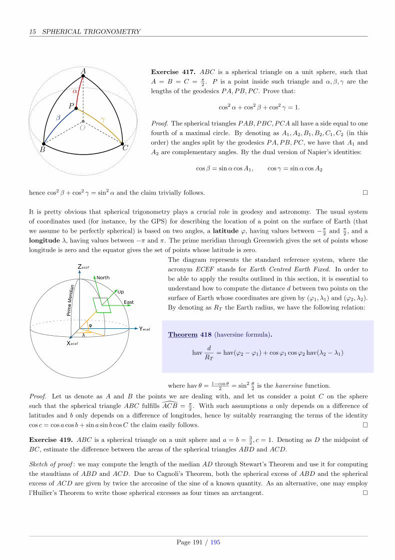
15 SPHERICAL TRIGONOMETRY
Exercise 417. ABC is a spherical triangle on a unit sphere, such that
A = B = C = π2 . P is a point inside such triangle and α, β, γ are the
lengths of the geodesics PA,PB,PC. Prove that:
cos2 α+ cos2 β + cos2 γ = 1.
Proof. The spherical triangles PAB,PBC,PCA all have a side equal to one
fourth of a maximal circle. By denoting as A1, A2, B1, B2, C1, C2 (in this
order) the angles split by the geodesics PA,PB,PC, we have that A1 and
A2 are complementary angles. By the dual version of Napier’s identities:
cosβ = sinα cosA1, cos γ = sinα cosA2
hence cos2 β + cos2 γ = sin2 α and the claim trivially follows.
It is pretty obvious that spherical trigonometry plays a crucial role in geodesy and astronomy. The usual system
of coordinates used (for instance, by the GPS) for describing the location of a point on the surface of Earth (that
we assume to be perfectly spherical) is based on two angles, a latitude ϕ, having values between −π2 and π2 , and a
longitude λ, having values between −π and π. The prime meridian through Greenwich gives the set of points whose
longitude is zero and the equator gives the set of points whose latitude is zero.
The diagram represents the standard reference system, where the
acronym ECEF stands for Earth Centred Earth Fixed. In order to
be able to apply the results outlined in this section, it is essential to
understand how to compute the distance d between two points on the
surface of Earth whose coordinates are given by (ϕ1, λ1) and (ϕ2, λ2).
By denoting as RT the Earth radius, we have the following relation:
Theorem 418 (haversine formula).
havd
RT= hav(ϕ2 − ϕ1) + cosϕ1 cosϕ2 hav(λ2 − λ1)
where hav θ = 1−cos θ2 = sin2 θ
2 is the haversine function.
Proof. Let us denote as A and B the points we are dealing with, and let us consider a point C on the sphere
such that the spherical triangle ABC fulfills ACB = π2 . With such assumptions a only depends on a difference of
latitudes and b only depends on a difference of longitudes, hence by suitably rearranging the terms of the identity
cos c = cos a cos b+ sin a sin b cosC the claim easily follows.
Exercise 419. ABC is a spherical triangle on a unit sphere and a = b = 32 , c = 1. Denoting as D the midpoint of
BC, estimate the difference between the areas of the spherical triangles ABD and ACD.
Sketch of proof : we may compute the length of the median AD through Stewart’s Theorem and use it for computing
the staudtians of ABD and ACD. Due to Cagnoli’s Theorem, both the spherical excess of ABD and the spherical
excess of ACD are given by twice the arccosine of the sine of a known quantity. As an alternative, one may employ
l’Huilier’s Theorem to write those spherical excesses as four times an arctangent.
Page 191 / 195

We finish this section by mentioning an astonishing and very recent result, extending both Euler’s Theorem on the
collinearity of O,G,H and Feuerbach’s Theorem on the property of the nine-point-circle to the spherical case.
We say that in a spherical triangle ABC a cevian AD is a pseudoaltitude if it fulfills
BDA = DAB +B − E
2, CDA = CAD + C − E
2
with E being the spherical excess of ABC. Using the spherical version of Ceva’s Theorem it is not difficult to prove
that the pseudoaltitudes concur, at a point (not surprisingly) known as pseudoorthocenter. We have already proved
Steiner’s Theorem about the concurrency of the pseudomedians at the pseudocentroid.
Theorem 420 (Akopyan). In a spherical triangle the circumcenter, the pseudocentroid and the pseudoorthocenter
lie on the same geodesic. Additionally, the feet of the pseudoaltitudes and the midpoints of the sides belong to the
same circle, which is tangent to the inscribed circle and to every ex-inscribed circle.
Sketch of proof. It is not difficult to locate the positions, on the triangle sides, of the feet of the cevians through
the circumcenter, the pseudocentroid and the pseudoorthocenter. Then it is possible to employ the projective map
given by the central projection from the surface of the sphere to the plane πABC containing the vertices of ABC. The
first part of the statement follows from Van Obel’s and Ceva’s Theorems. The existence of a spherical analogue of
the nine points circle can be proved with a similar technique, i.e. by showing the concurrence of three perpendicular
bisectors on πABC . The last part of the statement is the most difficult to prove, but that can be done by invoking the
generalization of Ptolemy’s theorem known as Casey’s Theorem.
The material composing this section, up to minor changes due to the author, mainly comes from three sources:
1. John Casey, A Treatise in Spherical Trigonometry, Hodges, Figgis & co, Dublin 1889;
2. Ren Guo, Estonia Black, Caleb Smith, Strengthened Euler’s inequality in spherical
and hyperbolic geometries, ArXiv, 17/04/2017;
3. Arseniy V.Akopian, On some classical constructions extended to hyperbolic geometry,
ArXiv, 11/05/2011.
We invite the reader to have a look at them in order to acquire a broader view on the subject. Casey’s treatise, for
instance, is an impressive and very detailed work on spherical trigonometry, with the appearance of being a complete
compendium. However the research of new results in spherical geometry is far from being over: Akopyan’s Theorem,
proved more than a century after Casey’s treatise, is exemplary, and many interesting questions just arise from picking
a non-trivial result in Euclidean Geometry and wondering if it admits a spherical analogue.
Page 192 / 195

REFERENCES
Students interested in having one or more references among the following ones can contact me
at the address [email protected].
References
[1] Aigner, Ziegler, Proofs from The Book
[2] Ahlfors, Complex Analysis
[3] N.Alon, The Combinatorial Nullstellensatz
[4] K.Ball, An Elementary Introduction to Modern Convex Geometry
[5] Boros, Moll, Irresistible Integrals
[6] Borwein, Borwein, Pi and the AGM: A Study in Analytic Number Theory and Computational Complexity
[7] N.G. de Bruijn, Asymptotic Methods in Analysis
[8] N.L. Carothers, A Short Course on Approximation Theory
[9] C. Casolo, Corso di Teoria dei Grafi
[10] K. Chandrasekharan, Introduction to Analytic Number Theory
[11] Flajolet, Sedgewick, Analytic Combinatorics
[12] Flajolet, Salvy, Euler Sums and Contour Integral Representations
[13] D.M. Kane, An elementary derivation of the asymptotics of partition functions
[14] Konrad, Knopp, Theory and Applications of Infinite Series
[15] Ireland, Rosen, A Classical Introduction to Modern Number Theory
[16] Mitrinovic, Pecaric, Fink, Classical and New Inequalities in Analysis
[17] P. Nahin, Inside Interesting Integrals
[18] Petrushev, Popov, Rational Approximations of Real Functions
[19] M. Steele, The Cauchy-Schwarz Master Class
[20] Elias M. Stein, Fourier Analyis - an introduction
[21] G. Szego, On a inequality of P.Turan concerning Legendre polynomials
[22] A. Treibergs, Mixed Area and the Isoperimetric Inequality
[23] J.H. van Lint, R.M. Wilson, A course in Combinatorics
[24] Don Zagier, The Dilogarithm function
[25] Whittaker and Watson, A Course of Modern Analysis
[26] Herbert S. Wilf, Generatingfunctionology
Page 193 / 195

REFERENCES
Postscript.
The author is well-aware of the following flaws in these course notes:
• A debatable ordering of sections, such that if often happens that in section X something belonging to section
X + τ is used;
• A degree of malice in not presenting the minimal hypothesis allowing some manipulations, or a greater degree of
malice in not presenting hypothesis at all, and just using expressions like “as soon as everything makes sense”
or surrogates;
• To have declared this course as a problem solving omnibus in Calculus, Arithmetics, Algebra, Geometry and
Combinatorics, while this course is especially about Calculus and Combinatorics;
• To have included many exercises without worked solutions in a section they do not rightfully belong, according
to the usual strategies for solving them. I did this on purpose, so I guess I reach the maximum degree of malice
here.
I have several faults and some excuses. For starters, the spirit of these pages. F.Iandoli left a comment about them:
“It is a very personal piece of work, starting from the title itself. To do Superior Mathematics from an Elementary
point of view is a good summary of the author’s way for approaching Mathematics - we have a difficult problem. Well,
let’s bring it to its knees, by throwing the right amount of stones. Second point, the safeguard mechanism I activated
in the introduction: this chaotic collection of deep results and dirty tricks is not meant to be an institutional course,
but just as a compendium for young mathematicians, where to find interesting ideas in a concise form, interesting
exercises for getting better at problem solving and a (not so) small toolbox enlargement kit. Third point, the author
really loves not to take the usual way, and these notes are a bit of a challenge both for their writer (How could I
explain in the best possible way why these results are really important? ) and their readers (Here it is, in a single line,
a very difficult problem. If you reached this point, you can solve it, so solve it.) Anyway these pages will be improved
Page 194 / 195

REFERENCES
through time, maybe through their readers’ contributions, too. I am really grateful to Professor Massimo Caboara to
let me build this strange experiment in Mathematics education. My deep gratitude also goes to Greta Malaspina for
her several helpful comments and her collaboration in translating these course notes from Italian to English. I am also
greatly indebted to many users of Math.Stackexchange that contributed in some way to these notes: in no particular
order, achillehui, robjohn, Mike Spivey, Olivier Oloa, Mark Viola, Sangchul Lee, Vladimir Reshetnikov, Ron Gordon
and Tolaso J. Kos.
Jacopo D’Aurizio (aka Jack)
http://www.matemate.it
Page 195 / 195