© the mcgraw-hill companies, inc., 2005 2 -1 chapter 2 the complexity of algorithms and the lower...

2 -1

© The McGraw-Hill Companies, Inc., 2005

Chapter 2

The Complexity of Algorithms and the Lower Bounds

of Problems

2 -2


Measurement of the Goodness of an Algorithm

Time complexity of an algorithm worst-case average-case amortized

2 -3


NP-complete?

Measurement of the Difficulty of a Problem

2 -4


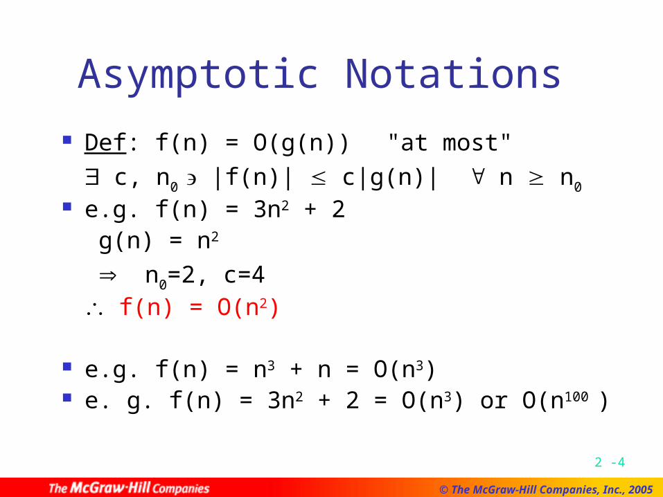
Asymptotic Notations Def: f(n) = O(g(n)) "at most"

c, n0 |f(n)| c|g(n)| n n0

e.g. f(n) = 3n2 + 2 g(n) = n2

n0=2, c=4 f(n) = O(n2)

e.g. f(n) = n3 + n = O(n3) e. g. f(n) = 3n2 + 2 = O(n3) or O(n100 )

2 -5


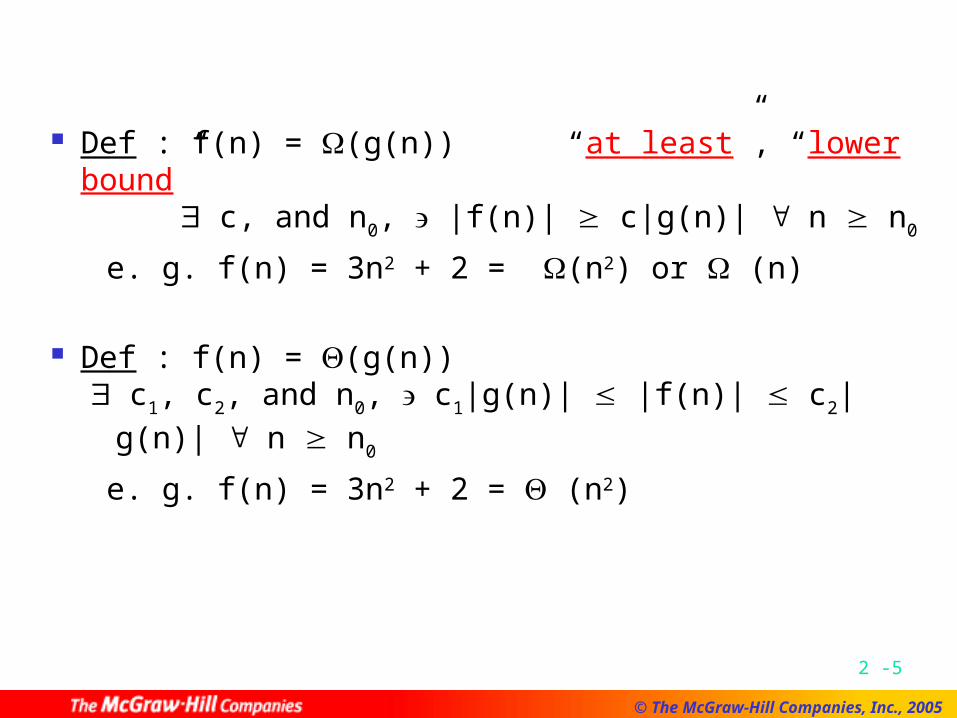
Def : f(n) = (g(n)) “at least”, “lower bound” c, and n0, |f(n)| c|g(n)| n n0

e. g. f(n) = 3n2 + 2 = (n2) or (n)

Def : f(n) = (g(n)) c1, c2, and n0, c1|g(n)| |f(n)| c2|g(n)| n n0

e. g. f(n) = 3n2 + 2 = (n2)

2 -6


Problem Size

Time Complexity Functions

10 102 103 104

log2n 3.3 6.6 10 13.3

n 10 102 103 104

nlog2n 0.33x102

0.7x103 104 1.3x105

n2 102 104 106 108

2n 1024 1.3x1030 >10100 >10100

n! 3x106 >10100 >10100 >10100

2 -7


Rate of Growth of Common Computing Time Functions

2 -8


O(1) O(log n) O(n) O(n log n) O(n2) O(n3) O(2n) O(n!) O(nn)

Common Computing Time Functions

2 -9


Any algorithm with time-complexity O(p(n)) where p(n) is a polynomial function is a polynomial algorithm. On the other hand, algorithms whose time complexities cannot be bounded by a polynomial function are exponential algorithms.

2 -10


Algorithm A: O(n3), algorithm B: O(n). Does Algorithm B always run faster than A?

Not necessarily. But, it is true when n is large enough!

2 -11


Analysis of Algorithms Best case Worst case Average case

2 -12


Straight Insertion Sort

input: 7,5,1,4,3 7,5,1,4,3 5,7,1,4,3 1,5,7,4,3 1,4,5,7,3 1,3,4,5,7

2 -13


Algorithm 2.1 Straight Insertion Sort

Input: x1,x2,...,xn

Output: The sorted sequence of x1,x2,...,xn

For j := 2 to n doBegin

i := j-1

x := xj

While x<xi and i > 0 do Begin

xi+1 := xi

i := i-1End

xi+1 := xEnd

2 -14


Inversion Table (a1,a2,...,an) : a permutation of {1,2,...,n} (d1,d2,...,dn): the inversion table of (a1,a2,...an) dj: the number of elements to the left of j that

are greater than j e.g. permutation (7 5 1 4 3 2 6) inversion table (2 4 3 2 1 1 0)

e.g. permutation (7 6 5 4 3 2 1) inversion table (6 5 4 3 2 1 0)

2 -15


M: # of data movements in straight insertion sort

1 5 7 4 3 temporary e.g. d3=2

1

1

)2(n

iidM

Analysis of # of Movements

2 -16


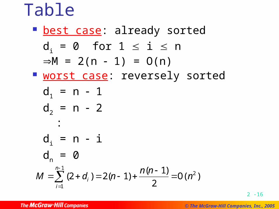
best case: already sorteddi = 0 for 1 i nM = 2(n 1) = O(n)

worst case: reversely sortedd1 = n 1d2 = n 2 :di = n i dn = 0

Analysis by Inversion Table

)O( 2

)1()1(2)2( 2

1

1

nnn

ndMn

ii

2 -17


average case: xj is being inserted into the sorted sequence x1 x2 ... x j-1

The probability that xj is the largest is 1/j. In this case, 2 data movements are needed.

The probability that xj is the second largest is 1/j . In this case, 3 data movements are needed.

: # of movements for inserting xj:

n

j

nnnj

M

j

j

j

jj

2

2 )O(4

)1)(8(

2

3

2

3132

2 -18


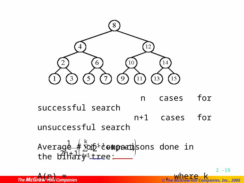
Binary Search

Sorted sequence : (search 9) 14 5 7 9 10 12 15

Step 1 Step 2 Step 3 best case: 1 step = O(1) worst case: (log2 n+1) steps = O(log n) average case: O(log n) steps

2 -19


n cases for successful search n+1 cases for unsuccessful search

Average # of comparisons done in the binary tree:

A(n) = , where k = log n+1

1

2 111

12

ni k ni

i

k

( )

2 -20


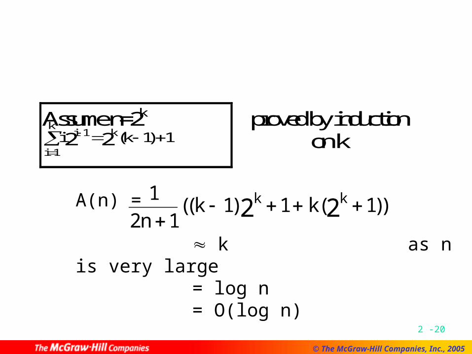
Assume n=2k

i ki k

i

k

1

12 2 1 1( )

proved by induction on k

A(n) =

k as n is very large = log n = O(log n)

1

2 11 1 12 2n

k kk k

(( ) ( ))

2 -21


Straight Selection Sort

7 5 1 4 31 5 7 4 31 3 7 4 51 3 4 7 51 3 4 5 7

We consider the # of changes of the flag which is used for selecting the smallest number in each iteration. best case: O(1) worst case: O(n2) average case: O(n log n)

2 -22


Quick Sort

Recursively apply the same procedure.

11 5 24 2 31 7 8 26 10 15 ↑ ↑

11 5 10 2 31 7 8 26 24 15 ↑ ↑

11 5 10 2 8 7 31 26 24 15 △ △ 7 5 10 2 8 11 31 26 24 15

|← <11 → | |← > 11 → |

2 -23


Best Case of Quick Sort Best case: O(n log n) A list is split into two sublists with almost e

qual size.

log n rounds are needed In each round, n comparisons (ignoring the

element used to split) are required.

2 -24


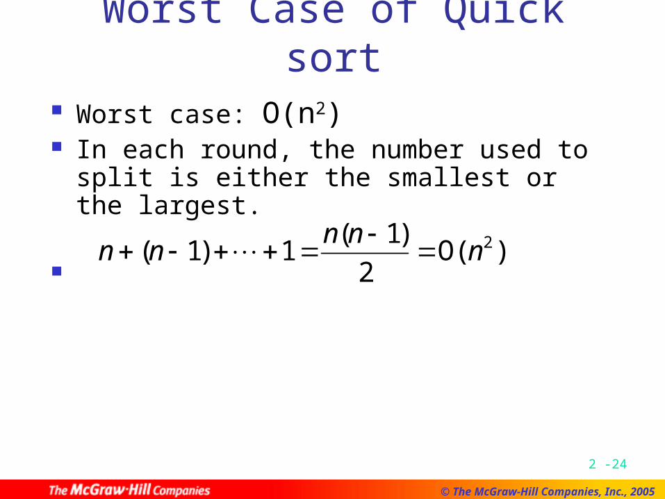
Worst Case of Quick sort Worst case: O(n2) In each round, the number used to split

is either the smallest or the largest.

)O(2

)1(1)1( 2n

nnnn

2 -25


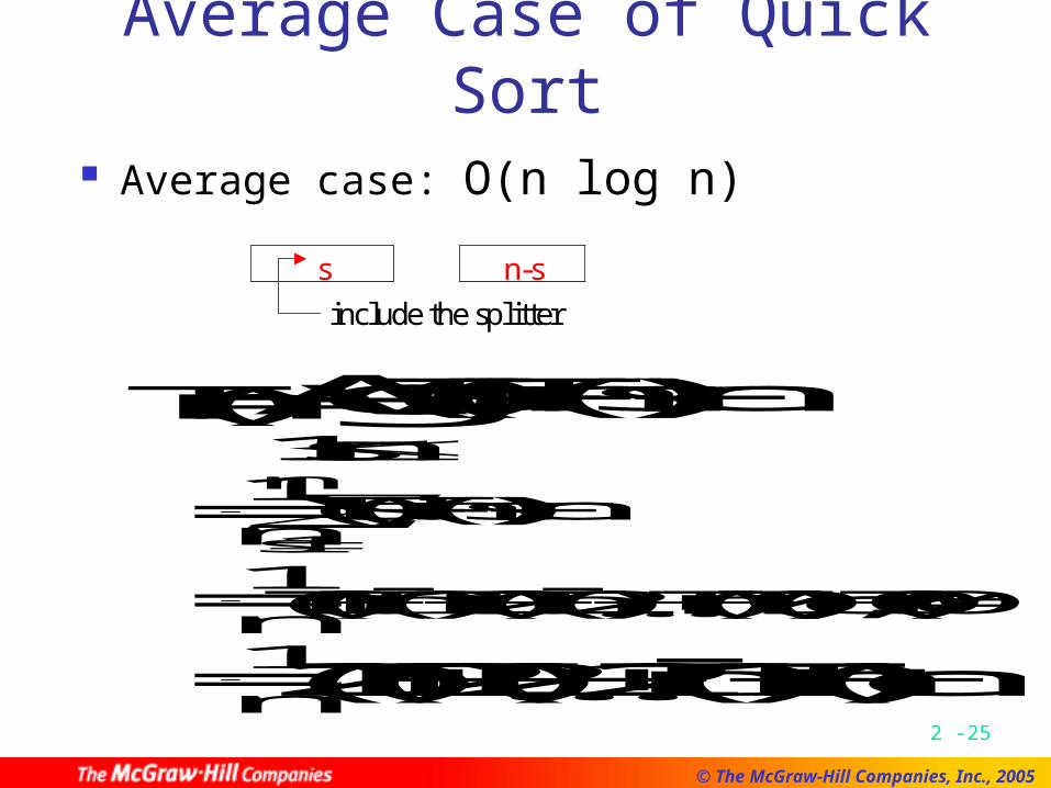
Average Case of Quick Sort

Average case: O(n log n)

s n-s

include the splitter

T(n) = 1

snAvgTsTnscn(()())

= 11nTsT(nscn

s

n(() ))

= 1n(T(1)+T(n1)+T(2)+T(n2)+…+T(n)+T(0))+cn, T(0)=0

= 1n(2T(1)+2T(2)+…+2T(n1)+T(n))+cn

2 -26


( n 1 ) T ( n ) = 2 T ( 1 ) + 2 T ( 2 ) + … + 2 T ( n 1 ) + c n 2 … … ( 1 ) ( n 2 ) T ( n - 1 ) = 2 T ( 1 ) + 2 T ( 2 ) + … + 2 T ( n 2 ) + c ( n 1 ) 2 … ( 2 ) ( 1 ) ( 2 ) ( n 1 ) T ( n ) ( n 2 ) T ( n 1 ) = 2 T ( n 1 ) + c ( 2 n 1 ) ( n 1 ) T ( n ) n T ( n 1 ) = c ( 2 n 1 )

T ( n

n

) = T ( n

nc

n n

1

1

1 1

1

)( )

= c ( 1 1

1n n

) + c ( 1

1

1

2n n

) + … + c ( 1

21 ) + T ( 1 ) , T ( 1 ) = 0

= c ( 1 1

1

1

2n n

. . . ) + c ( 1

1

1

21

n n

. . . )

2 -27


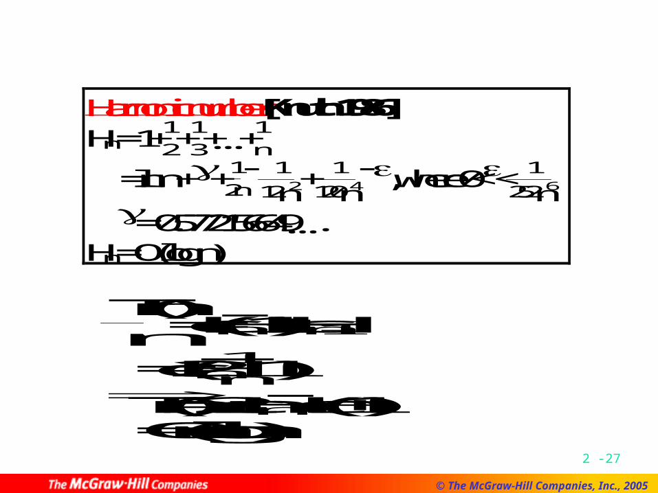
Harmonic number[Knuth 1986] Hn = 1+

1

2+1

3+…+1

n

=ln n + +1

2n 1

122n+1

1204n, where 0<<1

2526n

= 0.5772156649…. Hn = O(log n)

Tn

n

() = c(Hn1) + cHn-1

= c(2Hn1n1)

T(n) = 2 c n Hn c(n+1) =O(n log n)

2 -28


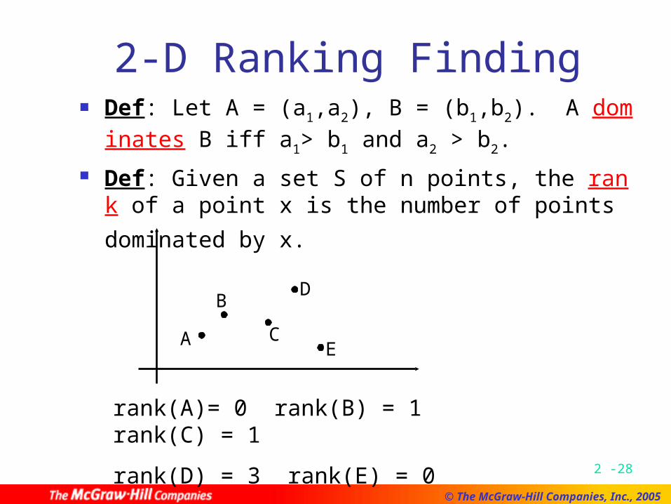
2-D Ranking Finding Def: Let A = (a1,a2), B = (b1,b2). A dominates B iff a1>

b1 and a2 > b2. Def: Given a set S of n points, the rank of a point x i

s the number of points dominated by x.

B

A C

D

E

rank(A)= 0 rank(B) = 1 rank(C) = 1

rank(D) = 3 rank(E) = 0

2 -29


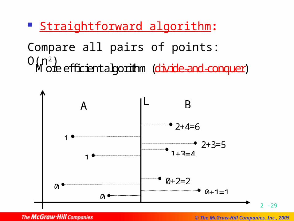
L

1+3=4

More efficient algorithm (divide-and-conquer)

A B

0+1=1

0+2=2

2+3=5

2+4=68 1

1

0

0

Straightforward algorithm:

Compare all pairs of points: O(n2)

2 -30


Step 1: Split the points along the median line L into A and B.

Step 2: Find ranks of points in A and ranks of points in B, recursively.

Step 3: Sort points in A and B according to their y-values. Update the ranks of points in B.

Divide-and-Conquer 2-D Ranking Finding

2 -31


Time complexity : step 1 : O(n) (finding median)

step 3 : O(n log n) (sorting) Total time complexity :

T(n) 2T( n

2) + c1 n log n + c2 n

2T( n

2) + c n log n

4T( n

4) + c n log n

2 + c n log n

nT(1) + c(n log n + n log n

2+n log n

4+…+n log 2)

= nT(1) + cn n nlog (log log ) 2

2

= O(n log2n)

2 -32


Lower Bound Def: A lower bound of a problem is the least time

complexity required for any algorithm which can be used to solve this problem.

☆ worst case lower bound ☆ average case lower bound

The lower bound for a problem is not unique. e.g. (1), (n), (n log n) are all lower bounds for

sorting. ((1), (n) are trivial)

2 -33


At present, if the highest lower bound of a problem is (n log n) and the time complexity of the best algorithm is O(n2). We may try to find a higher lower bound. We may try to find a better algorithm. Both of the lower bound and the algorithm may be

improved. If the present lower bound is (n log n) and

there is an algorithm with time complexity O(n log n), then the algorithm is optimal.

2 -34


The Worst Case Lower Bound of Sorting

6 permutations for 3 data elementsa1 a2 a3

1 2 31 3 22 1 32 3 13 1 23 2 1

2 -35


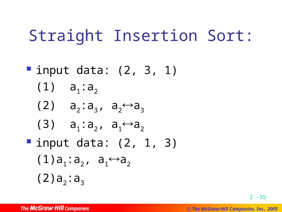
Straight Insertion Sort:

input data: (2, 3, 1)(1) a1:a2

(2) a2:a3, a2a3

(3) a1:a2, a1a2 input data: (2, 1, 3)

(1)a1:a2, a1a2

(2)a2:a3

2 -36


Decision Tree for Straight Insertion Sort

2 -37


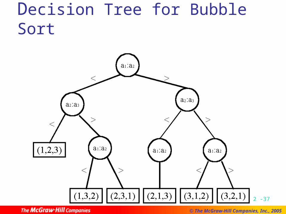
Decision Tree for Bubble Sort

2 -38


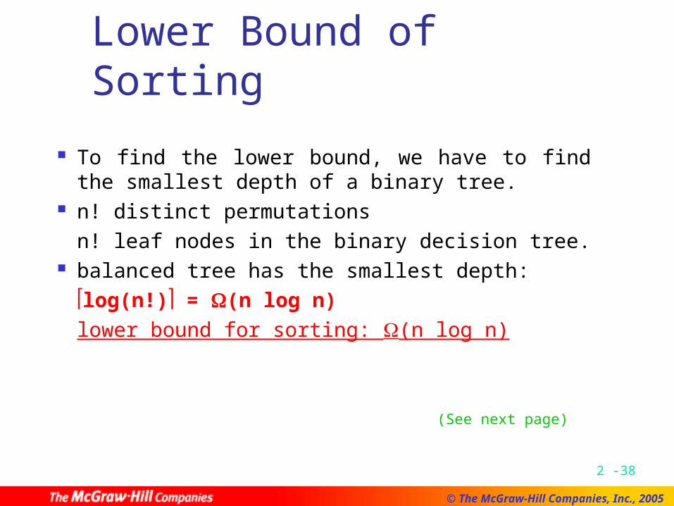
Lower Bound of Sorting

To find the lower bound, we have to find the smallest depth of a binary tree.

n! distinct permutationsn! leaf nodes in the binary decision tree.

balanced tree has the smallest depth:log(n!) = (n log n)lower bound for sorting: (n log n)

(See next page)

2 -39


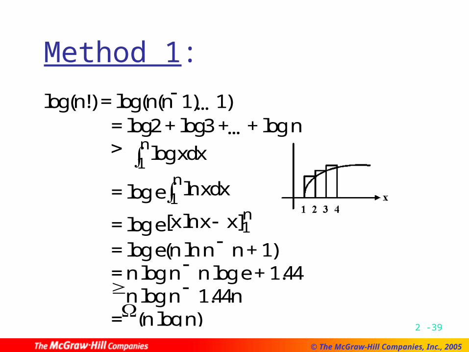
Method 1:

log(n!) = log(n(n 1)…1) = log2 + log3 +…+ log n

logxdxn1

= log e lnxdxn1

= log e[ ln ]x x x n 1 = log e(n ln n n + 1) = n log n n log e + 1.44 n log n 1.44n =(n log n)

2 -40


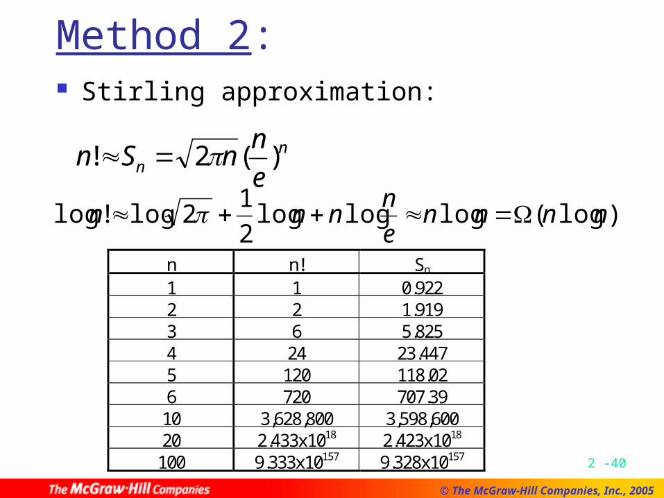
Method 2: Stirling approximation:

)log(logloglog2

12log!log nnnn

e

nnnn

n n! Sn 1 1 0.922 2 2 1.919 3 6 5.825 4 24 23.447 5 120 118.02 6 720 707.39

10 3,628,800 3,598,600 20 2.433x1018 2.423x1018

100 9.333x10157 9.328x10157

nn e

nnSn )(2!

2 -41


Heap Sort An optimal sorting algorithm

A heap: parent son

2 -42


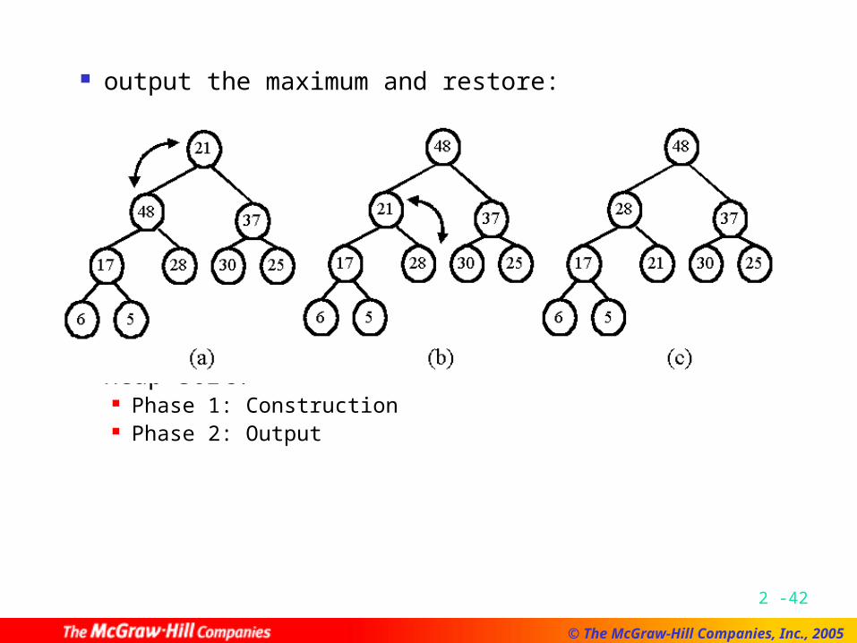
output the maximum and restore:

Heap sort: Phase 1: Construction Phase 2: Output

2 -43


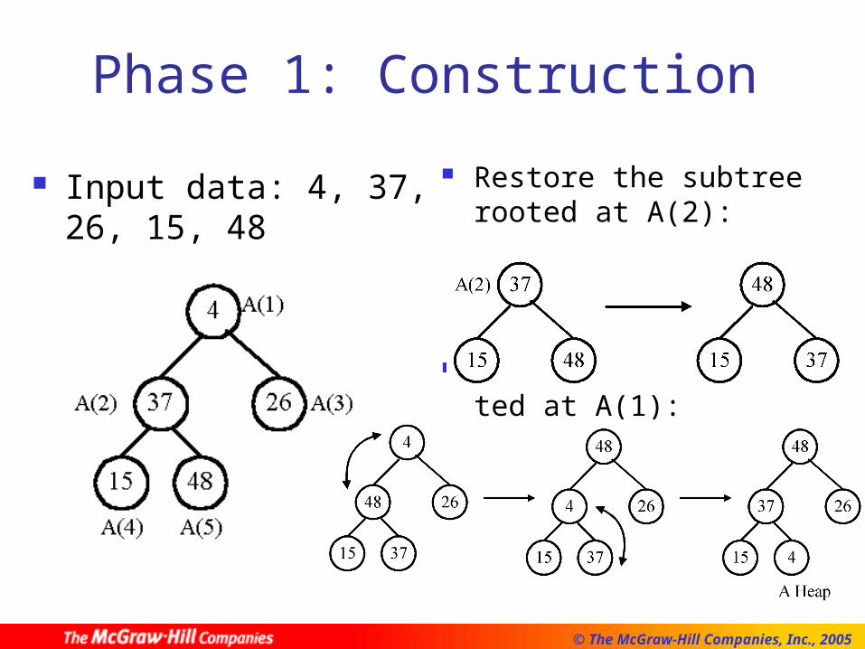
Phase 1: Construction

Input data: 4, 37, 26, 15, 48

Restore the subtree rooted at A(2):

Restore the tree rooted at A(1):

2 -44


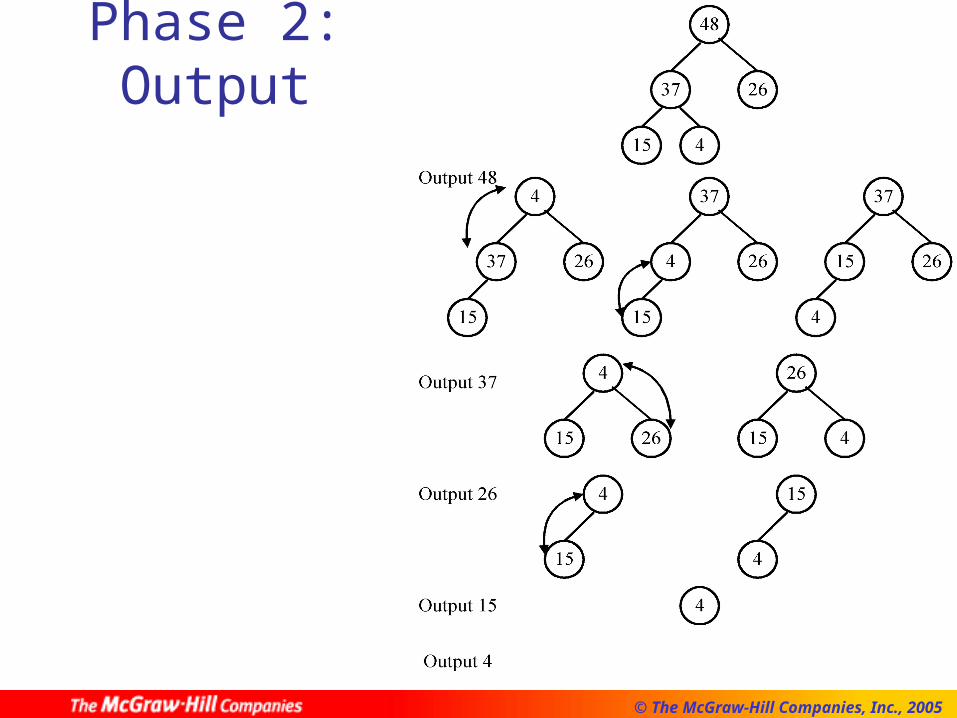
Phase 2: Output

2 -45


Implementation Using a linear array,

not a binary tree. The sons of A(h) are A(2h) and A(2h+1).

Time complexity: O(n log n)

2 -46


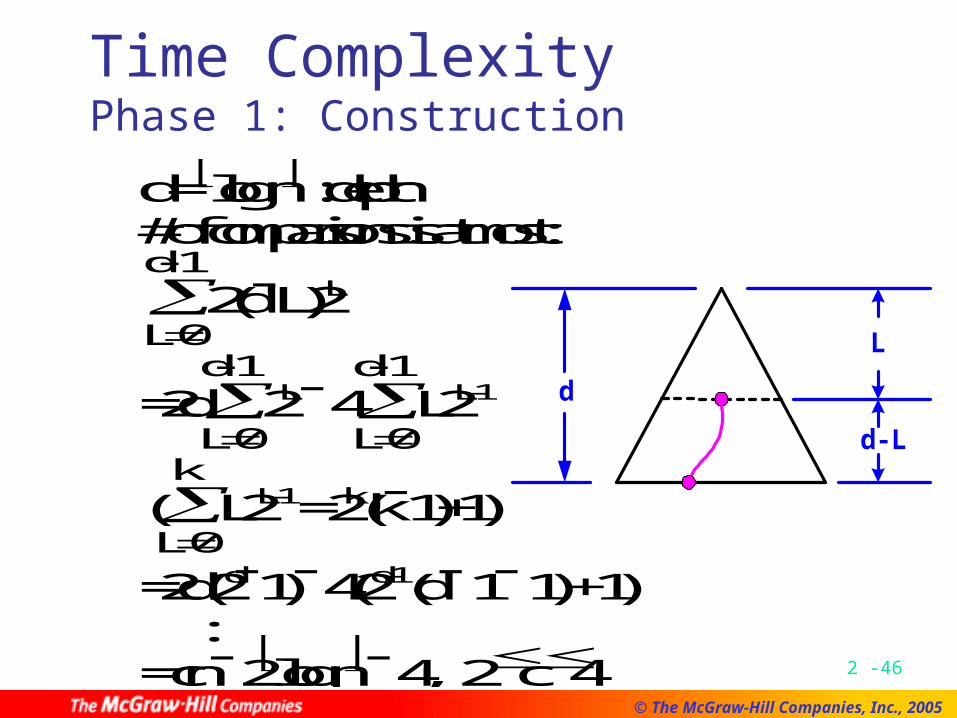
Time ComplexityPhase 1: Construction

d = log n : depth # of comparisons is at most:

L

d

0

12(dL)2L

=2dL

d

0

12L 4

L

d

0

1L2L-1

(L

k

0L2L-1 = 2k(k1)+1)

=2d(2d1) 4(2d-1(d 1 1) + 1) : = cn 2log n 4, 2 c 4

d

L

d-L

2 -47


Time Complexity Phase 2: Output

2i

n

1

1log i

= : =2nlog n 4cn + 4, 2 c 4 =O(n log n)

log ii nodes

max

2 -48


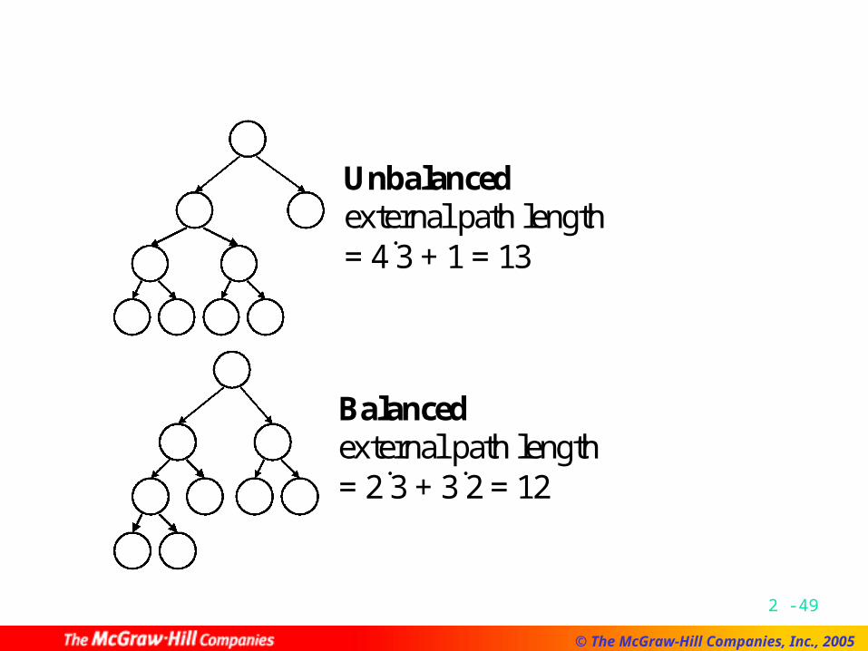
Average Case Lower Bound of Sorting

By binary decision trees. The average time complexity of a sorting

algorithm:The external path length of the binary tree

n! The external path length is minimized if

the tree is balanced.(All leaf nodes on level d or level d1)

2 -49


Unbalanced external path length = 43 + 1 = 13 Balanced external path length = 23 + 32 = 12

2 -50


Compute the Minimum External Path Length

1. Depth of balanced binary tree with c leaf nodes:

d = log c Leaf nodes can appear only on level d or

d1.2. x1 leaf nodes on level d1

x2 leaf nodes on level dx1 + x2 = c

x1 + = 2d-1

x1 = 2d c x2 = 2(c 2d-1)

x2

2

2 -51


3. External path length:

M= x1(d 1) + x2d = (2d 1)(d 1) + 2(c 2d-1)d = c(d 1) + 2(c 2d-1), d 1 = log c

= clog c + 2(c 2log c)4. c = n!

M = n!log n! + 2(n! 2log n!)M/n! = log n! + 2 = log n! + c, 0 c 1 = (n log n)

Average case lower bound of sorting: (n log n)

2 -52


Quick Sort Quick sort is optimal in the average

case.(O(n log n) in average)

2 -53


Heap Sort Worst case time complexity of heap

sort is O(n log n). Average case lower bound of

sorting: (n log n). Average case time complexity of

heap sort is O(n log n). Heap sort is optimal in the average

case.

2 -54


Improving a Lower Bound through Oracles

Problem P: merging two sorted sequences A and B with lengths m and n.

Conventional 2-way merging: 2 3 5 6 1 4 7 8 Complexity: at most m + n 1

comparisons

2 -55


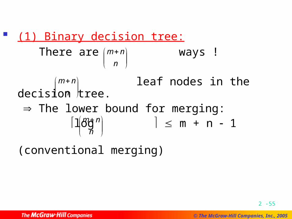
(1) Binary decision tree: There are ways !

leaf nodes in the decision tree. The lower bound for merging:

log m + n 1 (conventional merging)

n

nm

n

nm

n

nm

2 -56


When m = n

Using Stirling approximation

mmm

m

n

nmlog2))!2log((

)!(

)!2(loglog

2

n

e

nnn )(2!

12 )1(log2

12

)loglog2(log 2

)2

log22log2(loglog

mOmm

e

mmm

e

mmm

n

nm

Optimal algorithm: conventional merging

needs 2m 1 comparisons

2 -57


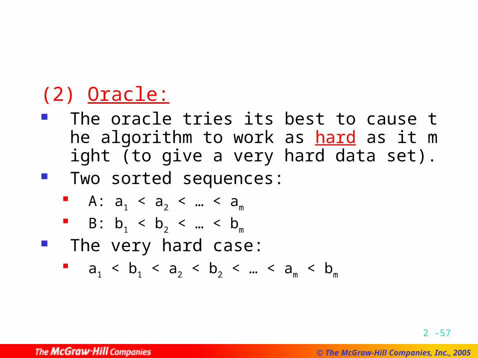
(2) Oracle: The oracle tries its best to cause the algori

thm to work as hard as it might (to give a very hard data set).

Two sorted sequences: A: a1 < a2 < … < am B: b1 < b2 < … < bm

The very hard case: a1 < b1 < a2 < b2 < … < am < bm

2 -58


We must compare:a1 : b1

b1 : a2

a2 : b2 :

bm-1 : am-1 am : bm

Otherwise, we may get a wrong result for some input data. e.g. If b1 and a2 are not compared, we can not distinguish

a1 < b1 < a2 < b2 < … < am < bm anda1 < a2 < b1 < b2 < … < am < bm

Thus, at least 2m1 comparisons are required. The conventional merging algorithm is optimal for m = n.

2 -59


Finding the Lower Bound by Problem Transformation

Problem A reduces to problem B (AB) iff A can be solved by using any algorithm

which solves B. If AB, B is more difficult.

Note: T(tr1) + T(tr2) < T(B) T(A) T(tr1) + T(tr2) + T(B) O(T(B))

instance of A

transformation T(tr1)

instance of B

T(A) T(B) solver of B

answer of A

transformation

T(tr2)

answer of B

2 -60


The Lower Bound of the Convex Hull Problem

Sorting Convex hull A B An instance of A: (x1, x2,…, xn)

↓transformationAn instance of B: {( x1, x1

2), ( x2, x2

2),…, ( xn, xn2)}

Assume: x1 < x2 < …< xn

2 -61


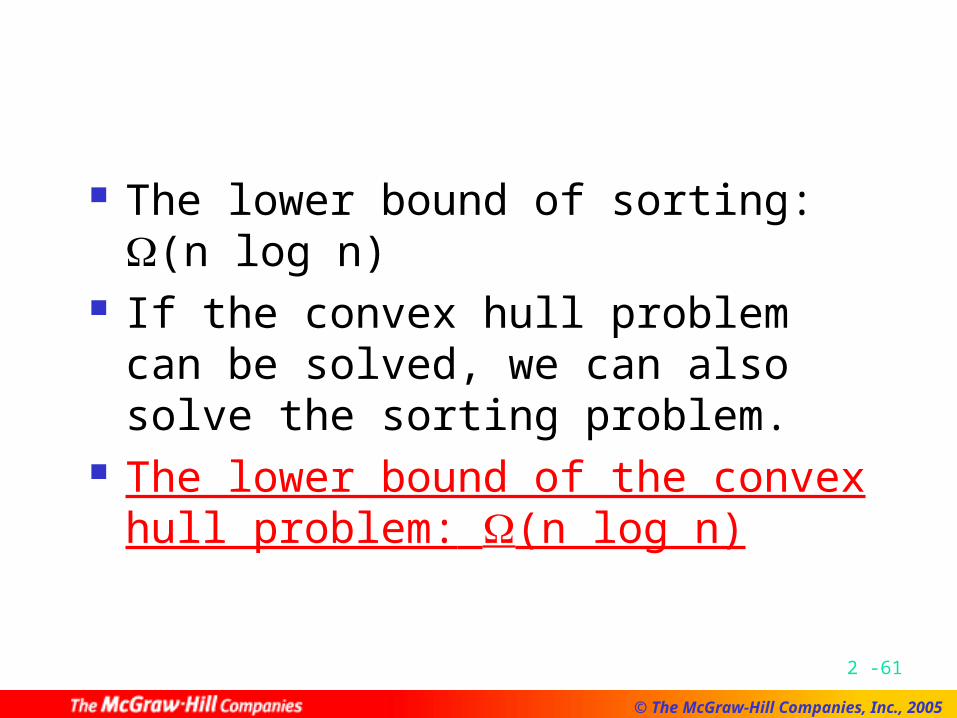
The lower bound of sorting: (n log n)

If the convex hull problem can be solved, we can also solve the sorting problem.

The lower bound of the convex hull problem: (n log n)

2 -62


The Lower Bound of the Euclidean Minimal Spanning Tree (MST)

Problem

Sorting Euclidean MST A B An instance of A: (x1, x2,…, xn)

↓transformationAn instance of B: {( x1, 0), ( x2, 0),…, ( xn, 0)} Assume x1 < x2 < x3 <…< xn.

There is an edge between (xi, 0) and (xi+1, 0) in the MST, where 1 i n1.

2 -63


The lower bound of sorting: (n log n)

If the Euclidean MST problem can be solved, we can also solve the sorting problem.

The lower bound of the Euclidean MST problem: (n log n)

© the mcgraw-hill companies, inc., 2005 2 -1 chapter 2 the complexity of algorithms and the lower...

Documents