sir20195073.pdf - u.s. geological survey publications ... · u.s. geological survey, reston,...
TRANSCRIPT
Sediment Classification and the Characterization, Identification, and Mapping of Geologic Substrates for the Glaciated Gulf of Maine Seabed and Other Terrains, Providing a Physical Framework for Ecological Research and Seabed Management
Scientific Investigations Report 2019–5073
U.S. Department of the InteriorU.S. Geological Survey


Sediment Classification and the Characterization, Identification, and Mapping of Geologic Substrates for the Glaciated Gulf of Maine Seabed and Other Terrains, Providing a Physical Framework for Ecological Research and Seabed Management
By Page C. Valentine
Scientific Investigations Report 2019–5073
U.S. Department of the InteriorU.S. Geological Survey

U.S. Department of the InteriorDAVID BERNHARDT, Secretary
U.S. Geological SurveyJames Reilly II, Director
U.S. Geological Survey, Reston, Virginia: 2019
For more information on the USGS—the Federal source for science about the Earth, its natural and living resources, natural hazards, and the environment—visit https://www.usgs.gov or call 1–888–ASK–USGS.
For an overview of USGS information products, including maps, imagery, and publications, visit https://store.usgs.gov.
Any use of trade, firm, or product names is for descriptive purposes only and does not imply endorsement by the U.S. Government.
Although this information product, for the most part, is in the public domain, it also may contain copyrighted materials as noted in the text. Permission to reproduce copyrighted items must be secured from the copyright owner.
Suggested citation:Valentine, P.C., 2019, Sediment classification and the characterization, identification, and mapping of geologic substrates for the glaciated Gulf of Maine seabed and other terrains, providing a physical framework for ecological research and seabed management: U.S. Geological Survey Scientific Investigations Report 2019–5073, 37 p., https://doi.org/10.3133/sir20195073.
ISSN 2328-0328 (online)

iii
Acknowledgments
The author thanks all those who participated on many research cruises to the waters of New England in collaboration with biologists of the National Marine Fisheries Service and the Stellwagen Bank National Marine Sanctuary. This report benefitted enormously from seabed mapping research generated by the Marine Geological and Biological Habitat Mapping (GEOHAB) community of scientists since the first meeting in 2001, and the author is especially grateful for discussions on this topic with Gary Greene (Moss Landing Marine Laboratories) and Brian Todd (Geological Survey of Canada). The author also thanks Dann Blackwood of the U.S. Geological Survey (USGS) who led the way in the collection of the seabed sediments and video imagery required to interpret the multibeam sonar survey data.


v
ContentsAcknowledgments ........................................................................................................................................iiiAbstract ...........................................................................................................................................................1Introduction.....................................................................................................................................................2Habitats Versus Substrates ..........................................................................................................................2
Definition of Habitat ..............................................................................................................................2Definition of Substrate .........................................................................................................................4
Classification of Sediment Grains by Size—Grades and Aggregates ..................................................4Classification of Naturally Occurring Sediments—Sediment Classes .................................................4Regional Setting .............................................................................................................................................8
Deglacial History ...................................................................................................................................8Seabed Topography and Present Hydrographic Conditions .........................................................9
Sediment Transport Processes and the Movement of Sediment Grains in the Region .....................9Sediment Resuspension and Transport Predicted by Analysis of the Effects of
Storm Wave and Tidal Currents on the Seabed .................................................................9Sediment Resuspension During Storms Documented by Sediment Trap Experiments ..........10
Data Types and Collection Methods .........................................................................................................11Results ...........................................................................................................................................................11
New, Simplified Classification of Sediment Grains by Size, Transport Mode, and Ecological Significance—Composite Grades ..................................................................11
Clay and Silt Aggregates Combined Into a Mud Composite Grade ...................................11Simplification of the Traditional Five-Grade Sand Classification Into Two
Composite Grades—Fine-Grained Sand and Coarse-Grained Sand ..................11Gravel Classified into Composite Grades by Grain-Size Analysis and by
Analysis of Seabed Imagery .......................................................................................12New Classification of Naturally Occurring Sediments—Sediment Classes ............................14Substrates are Characterized and Identified, Not Classified ......................................................15
Substrate Grain-Size Composition ..........................................................................................15Distribution of Grain Diameters in a Sediment .....................................................................15Measuring the Uniformity of the Distribution of Grain Diameters in a Sediment ...........15Substrate Mobility, Layering, and Structures .......................................................................16
Substrate Mapping .............................................................................................................................17Topographic Features, Ruggedness, and Sonar Backscatter Intensity of
the Seabed ....................................................................................................................17Presenting the Properties of Geologic Substrates ..............................................................18Depicting Boundaries of Mapped Substrates ......................................................................18Thematic Maps—Substrate Mobility, Fine- and Coarse-Grained Sand
Distribution, and Mud Content of Substrates ..........................................................18Substrate Symbols and Names ...............................................................................................18
Habitat Mapping..................................................................................................................................21Discussion .....................................................................................................................................................21References Cited..........................................................................................................................................23Sediment-Classification-Related Tables and Seabed Photographs ...................................................27

vi
Figures
1. Map showing locations of glaciated banks and basins and hydrographic processes in the Stellwagen Bank region east of Boston, Massachusetts .......................3
2. Table showing classifications of sediment grains, sediment grades, composite sediment grades, and sediment aggregates ............................................................................5
3. Triangular diagram showing grain-size composition of 15 classes of naturally occurring sediments based on weight percent of their aggregates (mud, sand, and gravel) content as determined by grain-size analysis ............................................................7
4. Cross sections of transect A, east-west, across Stellwagen Bank and into Stellwagen Basin with locations of sediment samples and the distribution of phi grain sizes relative to topography ............................................................................................13
5. Ternary diagram showing grain-size composition of 20 classes of naturally occurring sediments defined in this study based on weight percent of their aggregates (mud, sand, and gravel) content as determined by grain-size analysis .......14
6. Photographs of seabed substrates in the Stellwagen Bank region ..................................35 7. Map showing distribution of the backscatter intensity of geologic substrates
overlain on sun-illuminated topographic imagery in quadrangle 6 of the Stellwagen Bank National Marine Sanctuary region ...........................................................19
8. Map showing distribution of 10 geologic substrates overlain on sun-illuminated topographic imagery in quadrangle 6 of the Stellwagen Bank National Marine Sanctuary region ........................................................................................................................20
Tables
1. Definitions and origins of the terms sediment grade, composite sediment grade, sediment aggregate, sediment class, and substrate ..............................................................6
2. Grain-size analyses of suspended sediment collected on Georges Bank in 1978–79 .........................................................................................................................................10
3. Grain-size analyses of suspended sediment collected on Georges Bank in 1979–80 .........................................................................................................................................10
4. Grain-size analyses of suspended sediment collected in Massachusetts Bay in 1989–90 .........................................................................................................................................10
5. Guidelines for naming and abbreviating the components of sediment and nonsediment classes and the properties of substrates .......................................................28
6. Classification of naturally occurring sediments (sediment classes) based on grain-size analysis ......................................................................................................................29
7. Classification of mixed, naturally occurring sediments (sediment classes) based on grain-size analysis ................................................................................................................31
8. Properties of mapped geologic substrates in quadrangle 6 of the Stellwagen Bank National Marine Sanctuary region ................................................................................33
9. Classification of naturally occurring sediments and nonsediments based on analysis of seabed imagery ......................................................................................................34
10. Location, water depth, and date of seabed photographs shown in figure 6 ....................34

vii
Conversion Factors
International System of Units to U.S. customary units
Multiply By To obtain
Length
centimeter (cm) 0.3937 inch (in.)millimeter (mm) 0.03937 inch (in.)meter (m) 3.281 foot (ft)meter (m) 1.094 yard (yd)kilometer (km) 0.5400 mile, nautical (nmi)
Area
square meter (m2) 10.76 square foot (ft2)square kilometer (km2) 0.2916 square nautical mile (nmi2)square kilometer (km2) 0.3861 square mile (mi2)
DatumElevation, as used in this report, refers to depth of water from sea level.


Sediment Classification and the Characterization, Identification, and Mapping of Geologic Substrates for the Glaciated Gulf of Maine Seabed and Other Terrains, Providing a Physical Framework for Ecological Research and Seabed Management
By Page C. Valentine
AbstractA geologic substrate is a surface or volume of sediment
or rock where physical, chemical, and biological processes occur, such as the movement and deposition of sediment, the formation of bedforms, and the attachment, burrowing, feed-ing, reproduction, and sheltering of organisms. Seabed map-ping surveys in the Stellwagen Bank region off Boston, Mas-sachusetts, from 1993 to 2004 have led to the development of a methodology for characterizing, identifying, and mapping geologic substrates. The resulting high-resolution interpre-tive maps (1:25,000) show the distribution of substrates in a glaciated terrain of banks and basins in water depths of 30 to 185 meters. Data sources used to characterize substrates are multibeam sonar bathymetric and backscatter imagery to document seabed topography and patterns of sediment and rock distribution, grain-size analyses of sediment samples to determine substrate composition, and video and photographic imagery of the seabed to aid in the interpretation of multi-beam sonar imagery and to provide information on substrate layering and mobility, seabed structures, and sediments and nonsediment materials that cannot be physically sampled.
Sediment composition is a major property of many seabed substrates. Sediment grains belong to a continuum of grain-diameter sizes previously classified into grades (for example, fine sand, medium sand) and into aggregates (mud, sand, gravel). The definition of grade and aggregate boundaries in a classification is arbitrary, and a useful classification is limited to as few classes as are needed to effectively organize and apply information. For the purpose of mapping substrates, sediment grades and aggregates were simplified and re-classified into eight composite grades based on grain-size content, mode of transport, and ecological role. Five composite grades are identified using grain-size analysis and three are identified using video and photographic imagery of the seabed.
Naturally occurring sediments contain various amounts of the aggregates mud, sand, and gravel. The separation of
naturally occurring sediments into sediment classes, based on grain-size analysis, requires that limits be set on the amount of mud, sand, and gravel each class contains. Fifteen previ-ously identified basic sediment classes provided interpretive information on sediment transport by emphasizing gravel content (a low 0.01-weight-percent threshold) and on win-nowing processes based on the sand-to-mud ratio. The present study recognizes 20 basic sediment classes that are combina-tions of aggregates in which the lower limits for recognition of mud and sand are 10 weight percent and of gravel, 25 weight percent. These sediment classes can be made more specific by listing their content of the composite grades fine-grained sand (3 and 4 phi), which is transported in suspension, and coarse-grained sand (0, 1, and 2 phi), which is transported as bedload. Additional sediment classes and nonsediment classes that can-not be sampled are recognized on the basis of visual analysis of seabed video and photographic imagery and include pebble, cobble, and boulder gravel, rock outcrops, and shell beds, among others.
Substrates are not classified because their properties are too varied for a classification to be concise and useful. Rather, substrates are characterized and identified by sediment grain-size composition (the sediment class); the distribution, in millimeters, of grain diameters in the sediment; the pres-ence of nonsediments (for example, rock outcrops); substrate mobility based on the presence of sediment ripples; substrate layering (for example, a partial veneer of sand on gravel); and seabed structures. These properties have interpretive value by providing information about sedimentary processes acting on a substrate and about its ecological function. A geologic substrate, when it is associated with one or more species, is an important element of a habitat.
This methodology was developed to map a glaciated terrain characterized by geologic substrates that typify a wide range of erosional and depositional sedimentary environ-ments, and it likely will be useful for mapping substrates in other terrains. Substrate maps provide the physical frame-work required for identifying sediment transport processes,

2 Sediment Classification and the Mapping of Geologic Substrates for the Glaciated Gulf of Maine Seabed
validating sediment transport models, studying the ecology of species and communities, and managing marine resources and seabed usage.
IntroductionThe development of modern methods for imaging and
sampling sea floor environments has made it possible to cre-ate high-resolution interpretive maps of seabed properties. Although advanced multibeam sonar systems produce bathy-metric and backscatter imagery that show seabed features in great detail, physical sampling is still required to provide the groundtruth information needed to interpret the imagery and identify geologic substrates. A major goal of seabed analysis is to describe and map geologic substrates in a manner that improves our understanding of the relation between the physi-cal properties of the seabed and the species that use it. Sub-strates occur in a wide variety of ecological settings, and the term substrate has meaning for biologists who study relations between organisms and their environments. Once described and mapped, substrate properties will provide the physical framework necessary for studying the ecology of benthic spe-cies and communities and for managing the seabed.
This report presents a modified approach to seabed classification as described by Valentine and others (2005) by focusing on the characterization of geologic substrates alone, not on habitats. The principles described here for character-izing substrates were developed by mapping quadrangle 6 of the Stellwagen Bank National Marine Sanctuary region (fig. 1),1 a heterogeneous, glaciated bank and basin terrain of 211 square kilometers (km2) off Boston, Massachusetts. The diversity of seabed properties in this quadrangle make it an area suitable for developing a methodology to characterize and map substrates. Quadrangle 6 (Valentine and Gallea, 2015) is composed of 10 substrates that range from muddy sand to immobile sand to rippled sand to boulder ridges in water depths of 30 to 185 meters (m). A similar mapping effort is being applied to a wider region of the Gulf of Maine, includ-ing quadrangle 5 to the west.
The substrate characterization process utilizes informa-tion from a suite of physical properties that are common to substrates, including sediment grain-size composition and distribution of grain diameters, nonsediments (for example, rock outcrops), substrate mobility as determined by the pres-ence of sediment ripples, substrate layering (for example, an upper rippled sand substrate partially veneering a lower gravel substrate), and seabed structures (for example, burrows, bedforms, boulder piles). This information is acquired through grain-size analysis of sediment samples and visual interpreta-tion of multibeam sonar, video, and photographic imagery of the seabed. The mapping process resulted in the simplification
1Callouts to figures and tables have been hyperlinked to the location of the figure or table. Press and hold the Alt key followed by the left arrow key to return to the original page in the document after following the hyperlink.
of the grade classification of sediment grain sizes developed by Udden (1914) into fewer composite grades and the devel-opment of a new classification of naturally occurring sedi-ments into sediment classes that differ from those developed by Folk (1954, 1980).
This approach facilitates the characterization of geologic substrates and the determination of their potential ecological usage by organisms by using the newly defined composite grades for sand and gravel, placing less emphasis on gravel content than Folk (1954, 1980), and providing information on the mode of transport of the sand component (for example, fine-grained sand moves in suspension and coarse-grained sand is stationary or moves as bedload). It relies on video and photographic imagery to identify pebble, cobble, and boulder gravel and nonsediment substrates.
The compilation of substrate maps requires (1) charac-terization of substrates based on their physical properties and development of a suite of standard descriptors, (2) identifica-tion of substrates based on the presence of the descriptors, (3) mapping of geologic substrates, and (4) compilation of the-matic maps to show the physical properties of each substrate in terms of substrate mobility and the distribution of sand and mud content. The objective is to map substrates at a scale that provides information for a variety of uses that is justified by the resolution and density of sonar imagery, sediment grain-size analyses, and video and photographic observations. The mapping methodology developed for a heterogeneous, glaci-ated terrain should be also applicable to other terrains.
Habitats Versus Substrates
Definition of Habitat
It is useful to understand how the concepts of habitat and geologic substrate relate to each other. The definition of the fundamental ecological concept of “habitat” has varied over time. Charles Darwin (1872, p. 434) defined habitat as “the locality in which a plant or animal naturally lives.” This is interpreted here to mean that the “locality” is a geographic place whose environment allows a particular species or group of species to exist. Hall and others (1997) reviewed the use of habitat terminology in the scientific literature and concluded that “habitat is organism-specific” and should be defined “as the resources and conditions present in an area that produce occupancy … by a given organism.” This view is followed here. Dennis and others (2003, fig. 2) viewed habitat as func-tional and resource based and recognized that a species can reside in different habitats seasonally and use different areas of a habitat daily to perform the functions of feeding, breeding, sheltering, and migrating. For further discussion of the devel-opment of habitat definitions and terminology, see Dauvin and others (2008a, b), Elliott and others (2016), Olenin and Ducrotoy (2006), and references therein.

Habitats Versus Substrates 3
40
200
100
100
100100
80
80
80
80
40
80
80
40
10080
40
40
40
8
5
9
121110
4
1 2 3
1514
181716
13
7
6
D
C
E
A B
NMB
F, G
F
JEFFREYS LEDGE
TILLIES BANK
STELLWAG
EN BANK
STELLWAG
EN BANK
STELLWAGENBASIN
RACE POINT CHANNEL
Merr
imack River
CAPE COD BAY
CAPEANN
GULFOF
MAINE
CAPE COD
Plymouth
Provincetown
Gloucester
BOSTON
41°45'
42°45'
42°30'
42°15'
42°
71° 70°45' 70°30' 70°15' 70°
EXPLANATION
Stellwagen Bank National Marine Sanctuary
Major flow direction of semidiurnal tide
D, Flow direction of regional Maine Coastal Current
E, Wind direction of major storms from the northeast
F, Wave generated orbital seabed stress site (Butman and others, 2008)
G, Massachusetts Bay sediment trap site (Reid and others, 2005)
A, East-west grain-size distribution transect
B, Across the bankC, In Race Point Channel
Bathymetric contour—Contour interval is variable
MASSACHUSETTS
0 10 15 20 MILES5
0 20 KILOMETERS10 155
Study area
MA
Figure 1. Locations of glaciated banks and basins and hydrographic processes in the Stellwagen Bank region east of Boston, Massachusetts. The numbered grid outlines the U.S. Geological Survey substrate mapping project in the region that has been imaged using multibeam sonar technology. Cross sections of transect A are shown in figure 4. NMB, Ninety Meter Banks.

4 Sediment Classification and the Mapping of Geologic Substrates for the Glaciated Gulf of Maine Seabed
Definition of Substrate
A substrate is defined as “the substance, base, or nutri-ent on, or medium in which an organism lives and grows, or the surface to which a fixed organism is attached …” (Gary and others, 1972). Expanding on this definition, in this study a geologic substrate is defined as a surface or volume of sediment or rock where physical, chemical, and biological processes occur, such as the movement and deposition of sedi-ment, the formation of bedforms, and the attachment, burrow-ing, feeding, reproduction, and sheltering of organisms. The water column and its properties is a nongeologic substrate. A geologic substrate is but one element of an organism’s habitat, and, paraphrasing Hall and others (1997), it provides some of the resources and conditions that produce occupancy by a species.
Classification of Sediment Grains by Size—Grades and Aggregates
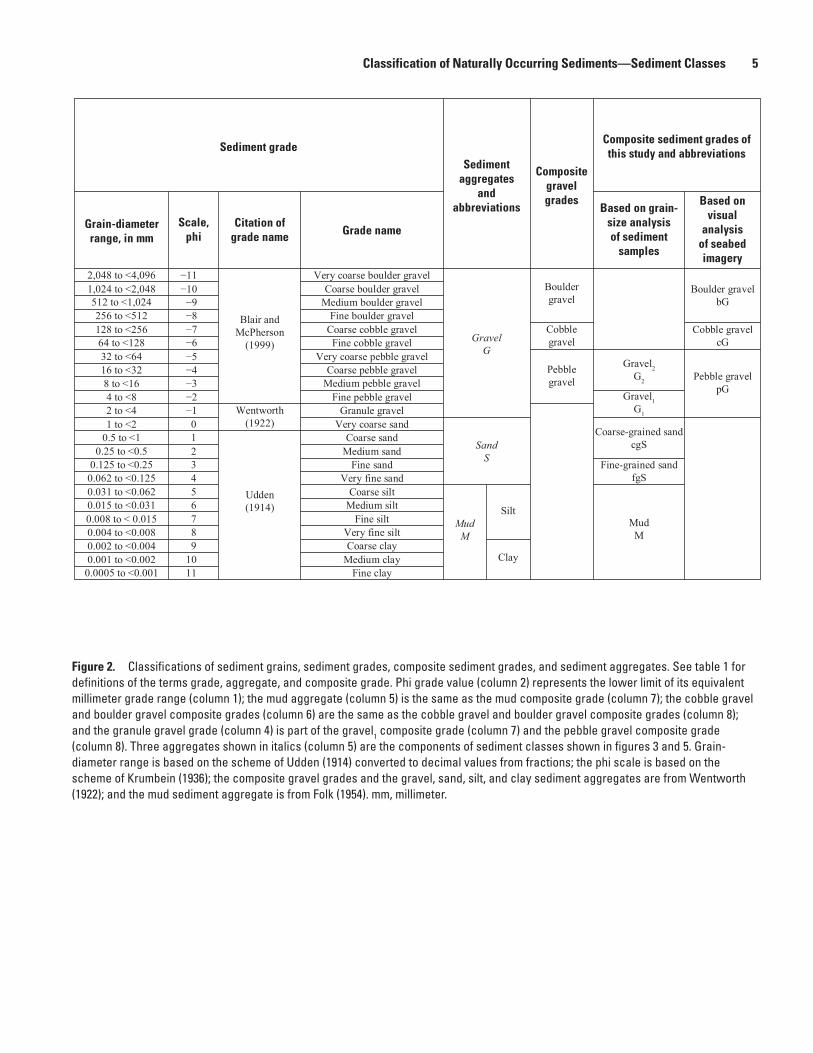
Classification is the process of arranging things (for example, sediment grains) into groups based on their prop-erties, and choices must be made as to how to define group boundaries. Udden (1914) classified clastic sediment grains by their grain diameters into 19 grades based on his arbitrary decision to double the grain-diameter range of each coarser grade (fig. 2; table 1). Udden’s sequence of grain diameters extends from 0.0005 to 256 millimeters (mm). Later, Blair and McPherson (1999) added four grades (extending from 256 to 4,096 mm) to the coarse end of the Udden classification, to give a total of 23 grades that range from clay particles to boulders. This is the standard for classifying sediment grains by size. The names of the sediment grades (for example, fine sand, coarse sand; see fig. 2, columns 3 and 4) have evolved since Udden’s initial proposal and now include names pro-posed by Udden (1914), Wentworth (1922), and Blair and McPherson (1999).
The grain-size boundaries of the Udden classification expressed in millimeters were converted by Krumbein (1936) into a sequence of whole numbers called phi (φ) values, where phi is the logarithm of the grain diameter (d) and is found using the formula φ = −log2d(mm) (fig. 2). An artefact of the phi grade classification that can confuse nongeologists is that grains >1 mm in diameter are expressed as negative phi values. For example, the granule gravel grade (2 to <4 mm) of Wentworth (1922) contains grains ranging from −1 to <−2 phi. Significantly, the phi grade scale conceals the doubling of the range of grain diameters (in millimeters) as sediments coarsen in the grade classification scheme of Udden (1914).
Wentworth (1922, tables 1 and 2) combined all sedi-ment grades defined at that time into four aggregates (clay, silt, sand, gravel) and subdivided the gravel aggregate into a granule gravel grade and three grades of pebble gravel, cobble gravel, and boulder gravel. The pebble, cobble, and
boulder gravel grades of Wentworth are here renamed com-posite grades (fig. 2) because they were later subdivided into 10 grades by Blair and McPherson (1999, fig. 2). Folk (1954) combined the clay and silt aggregates into the mud aggregate.
Classification of Naturally Occurring Sediments—Sediment Classes
The classification of naturally occurring sediments produces sediment classes (table 1), a major component of many seabed substrates. In designing a classification, it must be remembered that arbitrary choices are made to define class limits, and the purpose of the classification guides its structure. According to Wentworth (1922, p. 390) and Folk (1954, p. 345), a useful classification of naturally occurring sediments, based on grain-size analysis, should find a balance between being too simple (too few classes) and too complex (too many classes). Wentworth points out that the quantita-tive detail of the composition of each sediment class can be described better in tables than in verbal terminology.
Wentworth’s classification of naturally occurring sedi-ments contains 10 sediment classes defined by the weight percent content of the aggregates (clay, silt, sand, gravel) they contain and are named using two terms at most (Wentworth, 1922, p. 390). The weight percent content of each aggregate is treated equally by Wentworth in defining class boundaries. The lower limit for an aggregate to be included in a sediment class is >10 weight percent. For example, a sediment with gravel > sand > 10 weight percent, and other aggregates <10 percent, is a sandy gravel. His classification was not meant to be inclu-sive, and he did not include highly mixed sediments such as glacial till in his scheme.
Folk’s classification of naturally occurring sediments contains 15 sediment classes he called textural classes or textural groups (fig. 3) that, following Wentworth, are also defined by the weight percent content of the aggregates (mud, sand, gravel) they contain (Folk, 1954, fig. 1a, table 1; 1980, p. 25–28, table 1). Note that Folk combines silt and clay into a mud aggregate. By contrast with the Wentworth classification, which gives equal weight to clay, silt, sand, and gravel content, Folk designed sediment classes to reveal the effects of transport on sediment grains. The most important criterion is the gravel content, to emphasize its importance as an indicator of the velocity of the current from which the sediment was deposited. Sediments with only 0.01 to <5 weight percent gravel are classified as slightly gravelly, and sediments with ≥30 weight percent are classified as gravel. The second most important criterion is the sand-to-mud ratio that documents the effects of winnowing after deposition. The basic 15 sediment classes can be expanded to number several hundred by incorporating properties such as the median grain size of the gravel and sand fractions, the silt to clay ratio, and the degree of sorting of the sand classes (Folk, 1980, table 1).
Classification of Naturally Occurring Sediments—Sediment Classes 5
Sediment gradeSediment
aggregates and
abbreviations
Compositegravelgrades
Composite sediment grades ofthis study and abbreviations
Grain-diameterrange, in mm
Scale,phi
Citation ofgrade name Grade name
Based on grain- size analysisof sediment
samples
Based onvisual
analysisof seabedimagery
2,048 to <4,096 −11
Blair andMcPherson
(1999)
Very coarse boulder gravel
GravelG
Bouldergravel
Boulder gravelbG
1,024 to <2,048 −10 Coarse boulder gravel512 to <1,024 −9 Medium boulder gravel 256 to <512 −8 Fine boulder gravel128 to <256 −7 Coarse cobble gravel Cobble
gravel Cobble gravel
cG64 to <128 −6 Fine cobble gravel32 to <64 −5 Very coarse pebble gravel
Pebblegravel
Gravel2G2 Pebble gravel
pG
16 to <32 −4 Coarse pebble gravel8 to <16 −3 Medium pebble gravel4 to <8 −2 Fine pebble gravel Gravel1
G12 to <4 −1 Wentworth(1922)
Granule gravel1 to <2 0 Very coarse sand
SandS
Coarse-grained sandcgS 0.5 to <1 1
Udden(1914)
Coarse sand0.25 to <0.5 2 Medium sand
0.125 to <0.25 3 Fine sand Fine-grained sandfgS0.062 to <0.125 4 Very fine sand
0.031 to <0.062 5 Coarse silt
MudM
SiltMud
M
0.015 to <0.031 6 Medium silt0.008 to < 0.015 7 Fine silt 0.004 to <0.008 8 Very fine silt0.002 to <0.004 9 Coarse clay
Clay0.001 to <0.002 10 Medium clay0.0005 to <0.001 11 Fine clay
Figure 2. Classifications of sediment grains, sediment grades, composite sediment grades, and sediment aggregates. See table 1 for definitions of the terms grade, aggregate, and composite grade. Phi grade value (column 2) represents the lower limit of its equivalent millimeter grade range (column 1); the mud aggregate (column 5) is the same as the mud composite grade (column 7); the cobble gravel and boulder gravel composite grades (column 6) are the same as the cobble gravel and boulder gravel composite grades (column 8); and the granule gravel grade (column 4) is part of the gravel1 composite grade (column 7) and the pebble gravel composite grade (column 8). Three aggregates shown in italics (column 5) are the components of sediment classes shown in figures 3 and 5. Grain-diameter range is based on the scheme of Udden (1914) converted to decimal values from fractions; the phi scale is based on the scheme of Krumbein (1936); the composite gravel grades and the gravel, sand, silt, and clay sediment aggregates are from Wentworth (1922); and the mud sediment aggregate is from Folk (1954). mm, millimeter.

6 Sediment Classification and the Mapping of Geologic Substrates for the Glaciated Gulf of Maine Seabed
Table 1. Definitions and origins of the terms sediment grade, composite sediment grade, sediment aggregate, sediment class, and substrate.
[Refer to the text for further explanation and to figure 2 for grain-size ranges of grades, composite grades, and aggregates]
Term Definition and origin
Sediment grade A group of sedimentary grains (identified by grain-size analysis) that is part of a classification sequence of 23 grades each of whose grain-size range, in millimeters, doubles as grain diameters increase (a scheme developed by Udden, 1914). Grades based on this scheme were named by Udden (1914), Wentworth (1922), and Blair and McPherson (1999). Grades expressed in millimeters were converted to the phi scale by Krum-bein (1936). The phi grade scale conceals the doubling of the range of grain diameters in the millimeter grade classification. Grades are based on grain size only; they do not necessarily have interpretive meaning. It is unlikely that a naturally occurring sediment, described as a sediment class (see below), is represented by just one grade.
Composite sediment grade A term proposed here to describe a group of sedimentary grains formed by combining two to seven sediment grades into composite sediment grades (fig. 2) to simplify the grade classifications of Udden (1914), Wen-tworth (1922), and Blair and McPherson (1999), and to add interpretive meaning to the classification (for example, coarse-grained sand moves as bed load, and fine-grained sand moves as suspended load). Note that the pebble, cobble, and boulder gravel grades of Wentworth (1922, tables 1 and 2) are renamed composite grades because they were subdivided into 10 grades (fig. 2) by Blair and McPherson (1999, fig. 2). Ex-amples of composite sediment grades identified by grain-size analysis are mud (seven grades), fine-grained sand (two grades), coarse-grained sand (three grades), gravel1 (two grades), and gravel2 (three grades). Examples of composite sediment grades based on visual analysis of seabed imagery are pebble gravel (five grades), cobble gravel (two grades), boulder gravel (four grades). Composite sediment grades can occur as sediment classes.
Sediment aggregate Sediment grades were grouped into one of four aggregates: clay, silt, sand, and gravel by Wentworth (1922). Clay and silt were combined into the mud aggregate by Folk (1954). Aggregates can occur as naturally occurring sediment classes. Aggregates have interpretive value (for example, mud and gravel grains move differently and play different ecological roles on the seabed).
Sediment class A natural mixture of sediment grains. A sediment class (based on grain-size analysis) is not defined by a speci-fied range of grain sizes (as is a grade or an aggregate) but by the weight percents of the aggregates and composite grades it contains. Sediment classes have interpretive value. Wentworth (1922, p. 390) classified naturally occurring sediments into 10 sediment classes. He defined the classes by the weight percent of each of four aggregates (clay, silt, sand, gravel) in the sediment. Folk (1954, table 1; 1980, p. 25–28) classified natural sediments into fifteen textural classes based on the weight percent of three aggregates (mud, sand, gravel) in the sediment (fig. 3). Folk’s classes can be modified and increased in number by adding terms that describe the median grain size of both the gravel and sand aggregates expressed in grade terms (for example, pebbly coarse sand), the ratio of silt to clay, and the degree of sorting.
In the substrate component of the Coastal and Marine Ecological Classification Standard (Federal Geographic Data Committee, 2012), Folk’s classes are renamed “substrate groups and subgroups,” but the definition of their sediment content is unchanged. The British Geological Survey (Long, 2006) and the European Marine Observation and Data Network (Kaskela and others, 2019) reduced Folk’s 15 sediment classes to as few as four to facilitate mapping seabed sediment distributions at scales of 1:250,000 and 1:1,000,000.
In this study, sediment classes are defined by the weight percent of their aggregates (mud, sand, gravel; fig. 5) and, when more specificity is needed, by the weight percent of their composite grades (fine- and coarse-grained sand, gravel1, gravel2; table 8). Sediment and nonsediment classes that cannot be sampled are identified based on qualitative visual analysis of seabed imagery. See tables 5 to 7 and 9 for full descriptions of sediment and nonsediment classes. Here, a sediment class is not a substrate; it is one of several properties used to characterize and identify a substrate.
Geologic substrate A surface or volume of sediment or rock where physical, chemical, and biological processes occur, such as the movement and deposition of sediment, the formation of bedforms, and the attachment, burrowing, feeding, reproduction, and sheltering of organisms. Substrate properties (descriptors) include: grain-size composi-tion (sediment class); distribution of grain diameters in the sediment; nonsediment class; substrate mobility; substrate layering; and seabed structures. Nongeologic descriptors characteristic of a seabed substrate that are useful in its identification and mapping, such as water depth, can be utilized as appropriate.

Classification of Naturally Occurring Sediments—Sediment Classes 7
(g)M (g)mS (g)S(g)sM
G
SandSand : Mud ratio
Mud
Gravel
30
1:9
0.015
9:11:1
sG
gS
M sM mS S
80Pe
rcen
t gra
vel
Mud increases Sand increases
gravelly
GravelgmSgM
msGmG
30
5
Figure 3. Triangular diagram showing grain-size composition of 15 naturally occurring sediments (textural classes of Folk, 1954, 1980) based on weight percent of their aggregates (mud, sand, and gravel) content as determined by grain-size analysis (some labels outside the triangle have been added). The threshold for the recognition of gravel is greater than or equal to 0.01 weight percent. The gravel axis is shown to scale except for the 0.01 value. The gravel axis is not shown to scale in Folk (1954, fig. 1a; 1980, p. 26). See Long (2006) and Kaskela and others (2019) for modifications of Folk’s sediment classes. M, mud; m, muddy; S, sand; s, sandy; G, gravel; g, gravelly; (g), slightly gravelly.
For example, a slightly gravelly muddy sand with modifiers becomes a poorly sorted, slightly pebbly, silty, medium sand.
The Folk (1954, 1980) classification of sediments is identical to the classification of “unconsolidated mineral substrate” of the Coastal and Marine Ecological Classifica-tion Standard (CMECS; Federal Geographic Data Committee, 2012). The CMECS retains all of the threshold values of mud, sand, and gravel content proposed by Folk for classifying sediments. The major difference between the two classifica-tions is the change in terminology that resulted by the renam-ing of Folk’s 15 sediment classes as CMECS substrate groups and subgroups (Federal Geographic Data Committee, 2012, p. 105–108, fig. 7.2).
Folk’s sediment classification has been simplified several times for the purpose of mapping European seabed sediments at regional scales of 1:250,000 and 1:1,000,000. The British Geological Survey (BGS) combined Folk’s 15 classes into 11 or 4 classes (Long, 2006, figs. 1–4). During this process, the lower limit for recognizing gravel was raised from the 0.01 weight percent of Folk to 1 and then to 5 weight percent, and the boundary between sandy mud and muddy sand was redefined. This approach deemphasized the gravel content of the sediment and emphasized the mud content.
The European Marine Observation and Data Network (EMODnet) uses a modified Folk classification, similar to that of the BGS described by Long (2006), for mapping seabed sediments at scales of 1:250,000 and 1:1,000,000 (Kaskela and
others, 2019, fig. 3). EMODnet simplified Folk’s 15 sediment classes into 6 or 4 classes and added a “rock and boulders” class. The EMODnet maps of the European seas show the distribution of sediments using the following five sediment classes: mud to muddy sand, sand, mixed sediment, coarse sediment, and rock and boulders (Kaskela and others, 2019, figs. 6 and 7).
Barnhardt and others (1998) designed a seabed “bottom type” classification of the Maine coastal region based primar-ily on interpretation of side-scan sonar imagery supplemented by limited groundtruthing using sediment sampling, coring, and video imagery collected by submersibles. This classifica-tion contains 16 bottom types composed of four components (rock, gravel, sand, mud) and was developed to allow mapping at a scale of 1:100,000 of a topographically irregular, glaciated seabed that is a mix of sediments and bedrock outcrops. The four components of the classified bottom types are given equal weight in this classification, similar to Wentworth’s (1922) approach. Seabeds are classified as rock, gravel, sand, or mud if one of these components composes >90 percent of the area of a mappable unit. Seabeds are classified as composite units if one of the four components makes up ≥50 percent and ≤90 percent and another component makes up <50 percent of the unit by area. For example, if sand constitutes ≥50 of a map unit by area and gravel <50 percent, the bottom type (symbol Sg) is termed “sand with subordinate gravel” (Barnhardt and others, 1998, fig. 2).

8 Sediment Classification and the Mapping of Geologic Substrates for the Glaciated Gulf of Maine Seabed
Regional Setting
Deglacial History
The deglacial history of the Gulf of Maine provides infor-mation necessary for interpreting the glacial origin and subse-quent modification of the seabed materials in the Stellwagen Bank region. The events described here follow reconstructions of the final deglaciation of the Gulf of Maine and Atlantic Canada by Shaw and others (2002, 2006) whose maps show the locations of glacier margins through time.
The Gulf of Maine is a large, deep embayment of the United States and Canadian coasts that is separated from the Atlantic Ocean by two large shallow banks (Georges Bank and Browns Bank) that form the continental shelf (Shaw and oth-ers, 2006, fig. 1). There is some evidence for pre-Wisconsinan glaciations in the Gulf of Maine region (Stone and Borns, 1986; Siegel and others, 2012). However, the topography of the gulf’s deep basins and bounding ridges is interpreted to have formed primarily by the eastward advance of the Wis-consinan Laurentide Ice Sheet and subsequently modified by processes of deglaciation.
The Laurentide Ice Sheet reached its maximum extent (the Last Glacial Maximum) approximately (~) 22 thousand years before present time (ka BP) on the shallow continental shelf that separates the Gulf of Maine from the deep waters of the Atlantic Ocean (Shaw and others, 2006, fig. 8). By 20 ka BP, the ice sheet margin was breaking up, receding westward by melting, and opening the gulf to the waters of the Atlantic Ocean. By 16 ka BP, the ice sheet margin was off the present coast of Massachusetts in the region of Stellwagen Bank (Shaw and others, 2006, figs. 9–11).
Diverse glacial features, which include lateral and end moraines, eskers, kettles, crevasse splays, ice fall deposits, and iceberg plow marks were observed in multibeam sonar imag-ery of the Stellwagen Bank region and described in a series of 18 topographic maps (fig. 1; Valentine and others, 2010). On the southeastern margin of Stellwagen Bank, lateral moraines and an ice fall deposit are present to a depth of ~180 m below present sea level in quadrangle 6 (fig. 1) and are interpreted here to have originated at the margin of the melting ice sheet at ~16 ka BP as mapped by Shaw and others (2006, fig. 11). The presence of these features supports the hypothesis of Oldale and others (1990) that the melting ice sheet was grounded, in contrast to the interpretation of Schnitker and others (2001) who hypothesized that the glacier receded from the Gulf of Maine as a floating ice shelf.
The most rapid period of deglaciation occurred from ~16.5 to ~7 ka BP (Lambeck and others, 2014). By 14 ka BP, the ice sheet margin had receded onto the present land area of southeastern Massachusetts, and the glacial features of the Stellwagen Bank region had their first submergence by the rising sea (Shaw and others, 2006, fig. 12). By 13 ka BP, the ice sheet margin had receded farther westward to the New England coastal uplands (Shaw and others, 2006, fig. 13),
and the present coastal region from Massachusetts to Maine, which had been depressed by the weight of the melted ice, was flooded by the sea and covered by glaciomarine mud deposited from meltwater (Bloom, 1963; Oldale and others, 1990). It is likely that this marine mud forms the floors of the present nearshore basins. It is not known whether this mud was also deposited on Stellwagen Bank; however, outcroppings of semiconsolidated, burrowed mud were observed on the bank during the present study but could not be sampled.
By 12 ka BP, the depressed, submerged New England coastal region experienced crustal rebound in response to removal of the ice load, which caused the rising of the seabed, the eastward retreat of the sea, and the lowering of sea level (Shaw and others, 2006, fig. 14). In addition, by 11 ka BP, in a further response to removal of the ice, a bulge in the Earth’s crust, which had formed in front of the ice sheet (the forebulge), migrated westward resulting in additional rise of the present coastal region and further fall of sea level (Barn-hardt and others, 1995). This caused the emergence of some nearshore areas, including Stellwagen Bank (Shaw and others, 2002, fig. 9).
The timing and magnitude of this lowstand of sea level and emergence of the bank seem to have varied along the pres-ent coastal region from Massachusetts in the south to Maine in the north. Oldale and others (1993) suggest that the lowstand along the Massachusetts coast occurred earlier, at ~12 ka BP, and reached ~45 m below present sea level. Barnhardt and others (1995), whose sea-level curve is better documented than that of Oldale and others, suggest the maximum sea level fall along the Maine coast occurred somewhat later, from 11 to 10.5 ka BP, and that sea level reached ~55 m below present sea level. Significantly, both interpretations indicate the low-stand caused the shallowest part of Stellwagen Bank (presently −20 m on the Southwest Corner) to be exposed to a height of ~25 to ~35 m above present sea level. The effect of the foreb-ulge ended after 10.5 ka BP, and eustatic sea level rose so that, by ~8 ka BP, the bank experienced its second submergence (Oldale and others, 1990; Barnhardt and others, 1995; Shaw and others, 2002, fig. 12).
In summary, the glaciated Stellwagen Bank region, espe-cially the bank itself, has experienced three periods of erosion associated with rising and falling sea levels since the Last Glacial Maximum. The region was eroded first ~14 ka BP by the rising sea that followed the westward-melting glacial front. The bank was eroded a second time at ~11 ka BP by a falling sea when crustal rebound and a westward-migrating forebulge caused the low-stand emergence, and a third time at ~8 ka BP by eustatic sea level rise that finally submerged it. During these three periods, submarine and subaerial erosive processes likely modified glacial features; altered the grain-size compo-sition of glacially derived sediment (often mixes of mud, sand, and gravel); and determined, in large part, the character of present-day substrates. In shallow water, substrates continue to be reworked by episodic storms from the northeast that affect the Stellwagen Bank seabed to a depth of ~50 m.
Sediment Transport Processes and the Movement of Sediment Grains in the Region 9
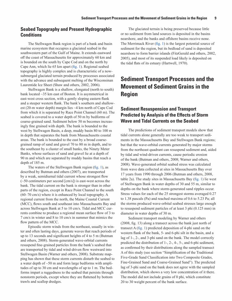
Seabed Topography and Present Hydrographic Conditions
The Stellwagen Bank region is part of a bank and basin marine ecosystem that occupies a glaciated seabed in the southwestern part of the Gulf of Maine. It extends eastward off the coast of Massachusetts for approximately 60 km and is bounded on the south by Cape Cod and on the north by Cape Ann, which lie 65 km apart (fig. 1). Regional seabed topography is highly complex and is characteristic of a now-submerged glaciated terrain produced by processes associated with the advance and subsequent melting of the Wisconsinan Laurentide Ice Sheet (Shaw and others, 2002, 2006).
Stellwagen Bank is a shallow, elongated (north to south) bank located ~35 km east of Boston. It is asymmetrical in east-west cross section, with a gently sloping eastern flank and a steeper western flank. The bank’s southern and shallow-est (20-m water depth) margin lies ~4 km north of Cape Cod from which it is separated by Race Point Channel (60 m). The seabed is covered to a water depth of 50 m by bedforms of coarse-grained sand. Sediment below 50 m becomes increas-ingly fine grained with depth. The bank is bounded to the west by Stellwagen Basin, a deep, muddy basin 80 to 100 m in depth that separates the bank from Massachusetts coastal areas. The bank is bounded to the east by a broad coarse-grained ramp of sand and gravel 70 to 80 m in depth, and to the southeast by a cluster of small banks, the Ninety Meter Banks, whose surfaces of sand and gravel lie at a depth of 90 m and which are separated by muddy basins that reach a depth of 185 m.
The waters of the Stellwagen Bank region (fig. 1), as described by Butman and others (2007), are transported by a weak, semidiurnal tidal current whose strongest flow (~50 centimeters per second [cm/s]) is east-west across the bank. The tidal current on the bank is stronger than in other parts of the region, except in Race Point Channel to the south (60–70 cm/s) where it is enhanced by local topography. A regional current from the north, the Maine Coastal Current (MCC), flows south and southeast into Massachusetts Bay and across Stellwagen Bank at 5 to 10 cm/s. Tidal and MCC cur-rents combine to produce a regional mean surface flow of 3 to 7 cm/s in winter and 8 to 10 cm/s in summer that mimics the flow pattern of the MCC.
Episodic storm winds from the northeast, usually in win-ter and often lasting days, generate waves that reach periods of up to 13 seconds and significant heights of 4 to 5 m (Butman and others, 2008). Storm-generated wave-orbital currents resuspend fine-grained particles from the bank’s seabed that are transported by tidal and wind-driven flow westward into Stellwagen Basin (Warner and others, 2008). Substrate map-ping has shown that these storm currents disturb the seabed to a water depth of ~50 m and form large bedforms with ampli-tudes of up to 30 cm and wavelengths of up to 1 m. The bed-forms impart a ruggedness to the seabed that persists through nonstorm periods, except where they are flattened by bottom trawls and scallop dredges.
The glaciated terrain is being preserved because little or no sediment from land sources is deposited in the basins nearshore, and the banks and offshore basins receive none. The Merrimack River (fig. 1) is the largest potential source of sediment for the region, but its bedload of sand is deposited nearshore to form barrier islands (FitzGerald and others, 2002, 2005), and most of its suspended load likely is deposited on the tidal flats of its estuary (Hartwell, 1970).
Sediment Transport Processes and the Movement of Sediment Grains in the Region
Sediment Resuspension and Transport Predicted by Analysis of the Effects of Storm Wave and Tidal Currents on the Seabed
The predictions of sediment transport models show that tidal currents alone generally are too weak to transport sedi-ments in the Massachusetts Bay and Stellwagen Bank regions; but that the wave-orbital currents generated by major storms from the northeast quadrant can resuspend sediment and, aided by tidal and wind-driven currents, cause periodic erosion of the bank (Butman and others, 2008; Warner and others, 2008). Wave-generated orbital seabed stress was calculated from wave data collected at sites in Massachusetts Bay over 17 years from 1990 through 2006 (Butman and others, 2008, table 2a). The study sites in Massachusetts Bay (fig. 1) lie west of Stellwagen Bank in water depths of 30 and 55 m, similar to depths on the bank where storm-generated sand ripples occur. Stress values for each of the 25 strongest storms averaged 0.27 to 1.38 pascals (Pa) and reached maxima of 0.6 to 5.23 Pa; all the storms produced wave-orbital seabed stresses large enough to resuspend sediment particles of at least 3 phi (0.125 mm) in diameter in water depths of 30 m.
Sediment transport modeling by Warner and others (2008, fig. 13) along a transect across the bank just north of transect A (fig. 1) predicted deposition of 4-phi sand on the western flank of the bank, 5- and 6-phi silt in the basin, and a lag of 1-, 2-, and 3-phi sand on the bank. The model correctly predicted the distribution of 1-, 2-, 4-, 5-, and 6-phi sediment, as confirmed by their distributions along the sampled transect A of this study (see section “Simplification of the Traditional Five-Grade Sand Classification into Two Composite Grades, Fine-Grained Sand and Coarse-Grained Sand”). The predicted lag of 3-phi sand on the bank does not agree with the sampled distribution, which shows a very low concentration of it there. The model did not include grains of 0 phi, which constitute 20 to 30 weight percent of the bank surface.
10 Sediment Classification and the Mapping of Geologic Substrates for the Glaciated Gulf of Maine Seabed
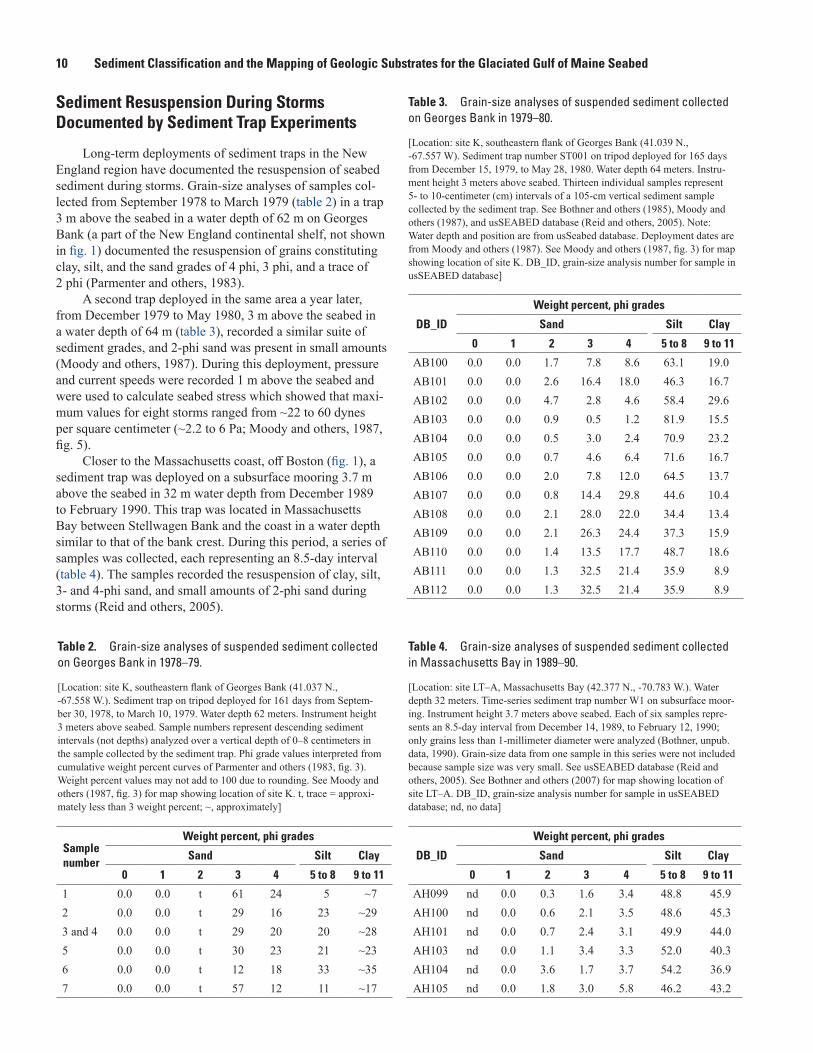
Sediment Resuspension During Storms Documented by Sediment Trap Experiments
Long-term deployments of sediment traps in the New England region have documented the resuspension of seabed sediment during storms. Grain-size analyses of samples col-lected from September 1978 to March 1979 (table 2) in a trap 3 m above the seabed in a water depth of 62 m on Georges Bank (a part of the New England continental shelf, not shown in fig. 1) documented the resuspension of grains constituting clay, silt, and the sand grades of 4 phi, 3 phi, and a trace of 2 phi (Parmenter and others, 1983).
A second trap deployed in the same area a year later, from December 1979 to May 1980, 3 m above the seabed in a water depth of 64 m (table 3), recorded a similar suite of sediment grades, and 2-phi sand was present in small amounts (Moody and others, 1987). During this deployment, pressure and current speeds were recorded 1 m above the seabed and were used to calculate seabed stress which showed that maxi-mum values for eight storms ranged from ~22 to 60 dynes per square centimeter (~2.2 to 6 Pa; Moody and others, 1987, fig. 5).
Closer to the Massachusetts coast, off Boston (fig. 1), a sediment trap was deployed on a subsurface mooring 3.7 m above the seabed in 32 m water depth from December 1989 to February 1990. This trap was located in Massachusetts Bay between Stellwagen Bank and the coast in a water depth similar to that of the bank crest. During this period, a series of samples was collected, each representing an 8.5-day interval (table 4). The samples recorded the resuspension of clay, silt, 3- and 4-phi sand, and small amounts of 2-phi sand during storms (Reid and others, 2005).
Table 2. Grain-size analyses of suspended sediment collected on Georges Bank in 1978–79.
[Location: site K, southeastern flank of Georges Bank (41.037 N., -67.558 W.). Sediment trap on tripod deployed for 161 days from Septem-ber 30, 1978, to March 10, 1979. Water depth 62 meters. Instrument height 3 meters above seabed. Sample numbers represent descending sediment intervals (not depths) analyzed over a vertical depth of 0–8 centimeters in the sample collected by the sediment trap. Phi grade values interpreted from cumulative weight percent curves of Parmenter and others (1983, fig. 3). Weight percent values may not add to 100 due to rounding. See Moody and others (1987, fig. 3) for map showing location of site K. t, trace = approxi-mately less than 3 weight percent; ~, approximately]
Sample number
Weight percent, phi grades
Sand Silt Clay
0 1 2 3 4 5 to 8 9 to 11
1 0.0 0.0 t 61 24 5 ~72 0.0 0.0 t 29 16 23 ~293 and 4 0.0 0.0 t 29 20 20 ~285 0.0 0.0 t 30 23 21 ~236 0.0 0.0 t 12 18 33 ~357 0.0 0.0 t 57 12 11 ~17
Table 3. Grain-size analyses of suspended sediment collected on Georges Bank in 1979–80.
[Location: site K, southeastern flank of Georges Bank (41.039 N., -67.557 W). Sediment trap number ST001 on tripod deployed for 165 days from December 15, 1979, to May 28, 1980. Water depth 64 meters. Instru-ment height 3 meters above seabed. Thirteen individual samples represent 5- to 10-centimeter (cm) intervals of a 105-cm vertical sediment sample collected by the sediment trap. See Bothner and others (1985), Moody and others (1987), and usSEABED database (Reid and others, 2005). Note: Water depth and position are from usSeabed database. Deployment dates are from Moody and others (1987). See Moody and others (1987, fig. 3) for map showing location of site K. DB_ID, grain-size analysis number for sample in usSEABED database]
DB_ID
Weight percent, phi grades
Sand Silt Clay
0 1 2 3 4 5 to 8 9 to 11
AB100 0.0 0.0 1.7 7.8 8.6 63.1 19.0AB101 0.0 0.0 2.6 16.4 18.0 46.3 16.7AB102 0.0 0.0 4.7 2.8 4.6 58.4 29.6AB103 0.0 0.0 0.9 0.5 1.2 81.9 15.5AB104 0.0 0.0 0.5 3.0 2.4 70.9 23.2AB105 0.0 0.0 0.7 4.6 6.4 71.6 16.7AB106 0.0 0.0 2.0 7.8 12.0 64.5 13.7AB107 0.0 0.0 0.8 14.4 29.8 44.6 10.4AB108 0.0 0.0 2.1 28.0 22.0 34.4 13.4AB109 0.0 0.0 2.1 26.3 24.4 37.3 15.9AB110 0.0 0.0 1.4 13.5 17.7 48.7 18.6AB111 0.0 0.0 1.3 32.5 21.4 35.9 8.9AB112 0.0 0.0 1.3 32.5 21.4 35.9 8.9
Table 4. Grain-size analyses of suspended sediment collected in Massachusetts Bay in 1989–90.
[Location: site LT–A, Massachusetts Bay (42.377 N., -70.783 W.). Water depth 32 meters. Time-series sediment trap number W1 on subsurface moor-ing. Instrument height 3.7 meters above seabed. Each of six samples repre-sents an 8.5-day interval from December 14, 1989, to February 12, 1990; only grains less than 1-millimeter diameter were analyzed (Bothner, unpub. data, 1990). Grain-size data from one sample in this series were not included because sample size was very small. See usSEABED database (Reid and others, 2005). See Bothner and others (2007) for map showing location of site LT–A. DB_ID, grain-size analysis number for sample in usSEABED database; nd, no data]
DB_ID
Weight percent, phi grades
Sand Silt Clay
0 1 2 3 4 5 to 8 9 to 11
AH099 nd 0.0 0.3 1.6 3.4 48.8 45.9AH100 nd 0.0 0.6 2.1 3.5 48.6 45.3AH101 nd 0.0 0.7 2.4 3.1 49.9 44.0AH103 nd 0.0 1.1 3.4 3.3 52.0 40.3AH104 nd 0.0 3.6 1.7 3.7 54.2 36.9AH105 nd 0.0 1.8 3.0 5.8 46.2 43.2
Results 11
Data Types and Collection Methods
The characterization and identification of seabed sub-strates requires the integration of areal geophysical data provided by multibeam sonar backscatter and bathymetric imagery of the seabed with groundtruth data provided by local video and photographic imagery and grain-size analyses of sediment samples. A bathymetric and backscatter survey of the Stellwagen Bank National Marine Sanctuary region (~3,780 km2) was conducted using a Simrad EM1000 multi-beam echosounder during 1994–6 in collaboration with the Canadian Hydrographic Service and the University of New Brunswick, Canada. The survey region was subdivided into 18 quadrangles (fig. 1), and several series of maps showing seabed topography, sun-illuminated topographic imagery, backscatter reflectivity, and ruggedness have been published, along with descriptions of survey and data processing meth-ods (Valentine, 2005; Valentine and others, 1998). Multibeam sonar data used in the present study are from quadrangle 6 (211 km2), a bank and basin terrain lying in water depths rang-ing from 30 to 185 m. Sediment grain-size analyses (325 sta-tions) and video and photographic imagery (288 stations) were acquired in 1993–6, 1998, 1999, 2003, and 2004 and used to interpret the features and seabed patterns observed in the sonar imagery (Valentine and Gallea, 2015). There have not been any multibeam sonar surveys since 1994–6, but video and photographic imagery and sediment samples collected into 2004 show that the substrate types described here did not change.
As part of the process of mapping the sea floor, the U.S. Geological Survey (USGS) developed the SEABed Observa-tion and Sampling System (SEABOSS) equipped with a grab sampler and cameras to collect sediment samples and video and photographic images of the seabed to aid in the inter-pretation of the sonar imagery (Valentine and others, 2000; Valentine and Gallea, 2015). The SEABOSS has a Van Veen sediment grab sampler mounted in the center of a frame that ensures the sampler is properly oriented on the seabed when a sample is collected. The upper 2 cm of sediment, representing the surface of the seabed, were removed from the sample with a rectangular shovel 2 cm deep and stored in a plastic bag for grain-size analysis that was performed at the USGS Woods Hole Coastal and Marine Science Center in Woods Hole, Mass., using a standard suite of analytical methods (Poppe and others, 2005). This laboratory has been in operation since 1963 and has analyzed many thousands of sediment samples collected by the USGS in New England.
Results
New, Simplified Classification of Sediment Grains by Size, Transport Mode, and Ecological Significance—Composite Grades
As described in the section “Classification of Sediment Grains by Size—Grades and Aggregates,” sediment grains historically have been classified into grades by grain size, with the range of grain diameters doubling for each coarser grade (fig. 2). This is accepted practice and provides a valuable stan-dard that makes the results of grain-size analyses comparable. It is the foundation from which new approaches to sediment classification can evolve. In this study, the mapping of geo-logic substrates is improved by re-classifying sediment grades into groups of grades referred to as “composite grades” (fig. 2; table 1) that are based not only on their grain-size content, but also on their mode of transport and ecological role.
Five composite grades that are identified by quantita-tive grain-size analysis are mud (silt and clay; 5 to 11 phi), fine-grained sand (3 and 4 phi), coarse-grained sand (0, 1, and 2 phi), gravel1 (−1 and −2 phi), and gravel2 (−3, −4, and −5 phi). Three composite grades that are identified by quali-tative visual analysis of seabed imagery are pebble gravel, including granules (−1 to −5 phi), cobble gravel (−6 and −7 phi), and boulder gravel (−8 to −11 phi).
Clay and Silt Aggregates Combined Into a Mud Composite Grade
Clay and silt grains consist of seven sediment grades (5 to 11 phi) whose maximum grain size is <0.062 mm (fig. 2). These grades were combined by Folk (1954) into a composite mud aggregate that simplified the classification of very small sedimentary particles. This study follows Folk; mud is treated as a composite grade consisting of clay and silt aggregates. Mud-size particles characteristically travel in suspension and are transported farther than larger grains, and they are deposited in the basins, the least energetic parts of the mapped region (Warner and others, 2008, fig. 13). The concept of “mud” is familiar to biologists and implies the occupancy of certain faunal types and the probable presence of burrows.
Simplification of the Traditional Five-Grade Sand Classification Into Two Composite Grades—Fine-Grained Sand and Coarse-Grained Sand
The 1994–6 multibeam echosounder survey of the central part of Stellwagen Bank revealed seabed structures (the lead-ing edges of rippled sand sheets) whose morphology indicated movement of sediment westward from the bank’s gently slop-ing eastern flank onto its more steeply sloping western flank

12 Sediment Classification and the Mapping of Geologic Substrates for the Glaciated Gulf of Maine Seabed
and into the deeper waters of Stellwagen Basin (Valentine, 2005, map B; Valentine, 2012; Valentine and others, 2010, quadrangle 5).
In the early stages of substrate characterization and iden-tification in this study, it became apparent that the weight per-cents of individual sediment grades in a sample were related to water depth. As was expected, the mud grades (>4 phi) were almost absent on the bank and most abundant in the deep water of the basins. Unexpectedly, the five sand grades were observed to segregate into two groups, with coarse phi grades (0, 1, and 2) being most abundant in samples at water depths <50 m on the bank, and fine phi grades (3 and 4) being most abundant between ~50 and ~90 m on the western flank of the bank. This observation suggests that these two sand groups represent different modes of transport, with 0-, 1-, and 2-phi sand being a lag deposit or moving as bedload, and 3- and 4-phi sand moving in suspension. This natural segregation of grades by grain size can be used to classify naturally occurring sediments and to characterize and identify substrates.
Plots of the grain-size distribution of 41 samples along transect A that extends from east to west across Stellwagen Bank into Stellwagen Basin (figs. 1 and 4) show an uneven distribution of individual phi grades related to water depth (see Valentine and others, 2010, for grain-size analysis data). At water depths shallower than ~50 m, the rippled bank surface is primarily coarse sediment (0, 1, 2 phi) and contains little fine sediment (3 phi, 4 phi, mud). At water depths between ~50 and ~90 m on the western flank, the unrippled seabed is domi-nantly 3-phi sand (~30 to ~55 percent) and 4-phi sand (~25 to ~50 percent). Mud, which is all but absent on shallower parts of the bank, increases to ~5 to ~25 percent in this depth inter-val. Below ~90 m, in the basin, mud is dominant (>90 weight percent) and all other phi grades are <1 percent, except for 4-phi sand which is <4 percent.
The formation of these texturally distinctive sediment deposits supports the interpretation that coarse sediment (0, 1, 2 phi) is stationary and (or) moves as bedload on the bank at water depths <~50 m; that fine sediment (3 phi, 4 phi, mud) is resuspended by wave-orbital storm currents in shallow parts of the bank and, aided by tidal and wind-driven currents, travels in suspension to the western flank (~50 to ~90 m) where it settles onto the seabed; and that most mud grains travel farther in suspension and settle in Stellwagen Basin at depths >90 m. The distribution of 2-phi sand (fig. 4B) indicates that a small amount of it is resuspended and settles onto the western flank.
These observations, and the results of the sediment trans-port studies described in the section “Sediment Transport Pro-cesses and the Movement of Sediment Grains in the Region” (especially the sediment trap experiments that documented the resuspension of mud and 3- and 4- phi sand to at least 3 m above the seabed during storms), led to a reclassification of the five sand grades on the basis of their modes of transport for the purpose of mapping substrates. Here, the grades (3 and 4 phi) that are resuspended and move in suspension are combined into a composite grade of “fine-grained sand,” and the grades (0, 1, and 2 phi) that remain on the seabed are combined
into a composite grade of “coarse-grained sand” (fig. 2). The proportions of each of the composite sand grades in a sample or substrate provide information on the modes of transport of the grains found in the sediment and on the kinds of organisms that can inhabit it.
Combining the traditional five sand grades into two com-posite grades is a key to the characterization, identification, and mapping of substrate types presented here. The observa-tion that fine-grained sand and coarse-grained sand move as described likely applies to any region where currents related to storms and tides resuspend and transport sediment. Exceptions likely are surf zones and areas that experience exceptionally strong tidal currents.
Gravel Classified into Composite Grades by Grain-Size Analysis and by Analysis of Seabed Imagery
The Van Veen sediment grab sampler used for collecting sediment samples in the Stellwagen Bank region rarely suc-cessfully collects gravel grains larger than pebbles (≥64-mm grain diameter). Therefore, a determination of the distribution of gravel in substrates requires two approaches, an evaluation of granule and pebble content (2 to <64 mm) by quantitative grain-size analysis of collected samples, where possible, and by a qualitative evaluation of the presence of pebbles, cobbles, and boulders through visual interpretation of seabed video and photographic imagery.
In this study, gravel grains between 2 and <64 mm in diameter (−1 to −5 phi) that can be sampled and then quantified by grain-size analysis are combined into two composite grades, gravel1 and gravel2 (fig. 2). This simplifies the characterization of these relatively small gravel grains without obscuring their possible ecological role as sites of biological attachment. The granule and fine pebble grades (−1 and −2 phi) are combined into composite grade gravel1 in which the largest grains are less than a centimeter (cm) in diameter. The smallest of these grades (granules, 2 to <4 mm) are only twice as large as very coarse sand, and it is likely that they and fine pebble gravel (4 to <8 mm) behave somewhat like sand grains insofar as they are unsuitable for the attachment of organisms. The three larger pebble grades (−3 to −5 phi) are combined into composite grade gravel2 that has a grain-diameter range of 8 to <64 mm, which is more likely to provide surface area suitable for attachment of organisms and conforms closely to the concept of gravel held by many nongeologists.
In general, the occurrence of the gravel grades and their potential ecological role in forming substrates can best be determined by an analysis of video and photographic imagery. This applies to the pebble gravel (2 to <64 mm) composite grade if it cannot be sampled and to the cobble gravel (64 to <256 mm) and boulder gravel (≥256 mm) composite grades. The pebble gravel composite grade includes granules and four pebble grades and is equivalent in grain size to combined

Results 13
1201101009080706050403020
0
20
40
60
80
100
Wat
er d
epth
, in
met
ers
Wei
ght p
erce
nt
1201101009080706050403020
Wat
er d
epth
, in
met
ers
Wei
ght p
erce
nt
1201101009080706050403020
0
20
40
60
80
100
0
20
40
60
80
100
0
20
40
60
80
100
0
20
40
60
80
100
Wat
er d
epth
, in
met
ers
Wei
ght p
erce
nt
1201101009080706050403020
Wat
er d
epth
, in
met
ers
Wei
ght p
erce
nt
1201101009080706050403020
70.4 70.3 70.2 70.1
Wat
er d
epth
, in
met
ers
Wei
ght p
erce
nt
Longitude west, in degrees
StellwagenBasin
Stellwagen Bank
A. 0 and 1 phiTransect A
EASTWEST
C. 3 phi
B. 2 phi
D. 4 phi
E. Mud
EXPLANATION
Water depth of the bank surface along42.3 degrees north latitude, in meters
Flank of the bank from 50- to 90-meter depth
Sediment sample, in weight percent
Figure 4. Cross sections of transect A, east-west, across Stellwagen Bank and into Stellwagen Basin with locations of sediment samples and the distribution of phi grain sizes relative to topography. A, 0 and 1 phi; B, 2 phi; C, 3 phi; D, 4 phi; and E, mud. Storm-wave currents from the northeast and east-west tidal currents resuspend and transport fine sediments from the bank onto the western flank and into Stellwagen Basin. Fine-grained sand (3 and 4 phi) and mud are deposited on the western flank.

14 Sediment Classification and the Mapping of Geologic Substrates for the Glaciated Gulf of Maine Seabed
gravel1 and gravel2 (fig. 2). The composite cobble gravel and boulder gravel grades in this study are equivalent to the com-posite cobble and boulder gravel grades of Wentworth (1922).
New Classification of Naturally Occurring Sediments—Sediment Classes
As classification is the process of arranging things into groups based on their properties, it follows that the more properties the things have, the more complex the classification will be. Sediment grains are classified by the increasing ranges of grain diameters into the grades of Udden (1914). Sediment grades are classified by combining them into the aggregates of Wentworth (1922) and Folk (1954). Naturally occurring sediments are classified by the weight percent content of their aggregates based on grain-size analysis (see section “Classifi-cation of Naturally Occurring Sediments—Sediment Classes”) to produce a more complex classification, the sediment classes of Wentworth (1922) and Folk (1954). Here, sediments are classified by the weight percent content of their aggregates and composite grades (figs. 2 and 5; table 1).
The new sediment classification is intended to improve the mapping of geologic substrates and to provide information on the potential ecological use of the substrates by organisms by (1) simplifying the properties of sediment classes by using
newly defined composite grades for sand and gravel; (2) plac-ing less emphasis than Folk (1954) on gravel content; (3) pro-viding information on the mode of transport of the sand com-ponent (for example, fine-grained sand moves in suspension and coarse-grained sand is stationary or moves as bedload); and (4) relying on video and photographic imagery to identify pebble, cobble, and boulder gravel.
In this classification of naturally occurring sediments, 20 basic sediment classes are defined by their aggregate (mud, sand, gravel) content based on grain-size analysis (fig. 5). Thirteen sediment classes have mud or sand or gravel content ≥50 weight percent (tables 5 and 6, in back of report). Seven classes of “mixed” sediment have mud, sand, and gravel content each <50 weight percent (table 7, in back of report). The lower limit for mud and sand to be included in a class is ≥10 weight percent of the sediment and for gravel ≥25 weight percent. The higher threshold for gravel assumes that sedi-ment collected with a grab sampler that contains <25 per-cent gravel will likely contain gravel grains that are too small (<64 mm diameter) and too sparse to be used by species for attachment or other purposes. The 20 basic sediment classes of this classification increase to 82 when they are modified by incorporating the weight percent of the composite grades fine- and coarse-grained sand they contain (tables 5–7, in back of report). The number of classes would also increase if the gravel content of composite grades gravel1 and gravel2 were to
MSG
sgM
G
sG
smG msG
mS
gS
S
gM
mG
sM
mgS
M
Percent gravel
Percent sand
Perc
ent m
ud
0
50
25
gravelly
Gravel
sandy Sand
Mud
mud
dy
SandMud
Gravel
MSSM
GSSGMG
GM
50
10
0 100
1000 10 50 100
Figure 5. Ternary diagram showing grain-size composition of 20 classes of naturally occurring sediments defined in this study based on weight percent of their aggregates (mud, sand, and gravel) content as determined by grain-size analysis. The threshold for recognition of mud or sand in a class is 10 weight percent and for gravel 25 percent. Outside the dashed line, 13 basic sediment classes are mud or sand or gravel. Inside the dashed line, 7 sediment classes are mixed mud and sand and gravel, but note that MSG represents one of six possible combinations of mud, sand, and gravel. See tables 6 and 7 for descriptions of the properties of sediment classes. M, mud; m, muddy; S, sand; s, sandy; G, gravel; g, gravelly.

Results 15
be included, but it would unnecessarily increase the complex-ity of class names. The gravel1 and gravel2 content can be better shown in tables that list substrate sediment composition (table 8, in back of report). The name of the sediment class (for example, muddy, gravelly, coarse-grained sand; mgcgS) that is an element of a substrate is indicated in a substrate’s name (see section “Substrate Symbols and Names” below).
Gravel and nonsediments such as rock, shell, or semicon-solidated mud that cannot be sampled constitute classes that are identified by visual analysis of seabed imagery (table 9, in back of report). No guidelines are provided here for estimating and classifying the areal extent of gravel and nonsediments.
Substrates are Characterized and Identified, Not Classified
In this study, substrates are not classified; they are charac-terized and identified based on their observed properties (their standard descriptors), which include grain-size composition (the sediment class described above), distribution of grain diameters, nonsediments (for example, rock outcrops), sub-strate mobility, substrate layering, seabed structures, and water depth (where defining). If substrates were to be classified, it would be necessary to classify each of the standard descrip-tors, which would produce a very large number of substrate classes and a complicated classification that likely would find little use.
Substrate Grain-Size Composition
The grain-size composition of a substrate, represented by its sediment class, is determined by grain-size analyses of sediment samples collected from the substrate and from analy-sis of video and photographic imagery of the seabed where samples cannot be collected. The number of possible identifi-able substrates depends on the number of sediment classes that are recognized by the sediment classification scheme. Fewer substrates will be identifiable if the sediment classification recognizes few sediment classes.
For a substrate that can be sampled, its grain-size com-position is defined by the mean weight percent of each of the two aggregates (sand, gravel) and five composite grades (mud, fine-grained sand, coarse-grained sand, gravel1, gravel2) it possibly contains (fig. 2; table 8, columns 7–13, in back of report). Mud, sand, and gravel are listed in the sediment class name in order of increasing weight percent.
For a substrate that cannot be sampled and must be analyzed using seabed imagery, its grain-size composition is defined by the presence of three composite grades of pebble gravel, cobble gravel, and boulder gravel it possibly contains (fig. 2) or by the presence of nonsediments, such as rock out-crop, shell deposit, and semiconsolidated mud. The terms peb-ble, cobble, and boulder in the class name indicate presence only; they are not listed in order of increasing areal coverage.
Distribution of Grain Diameters in a Sediment
A sediment can be characterized by the distribution of grain diameters that constitute most of its particles. “Sort-ing” is a measure of the uniformity of the distribution of grain diameters in a sediment, and the degree of sorting can be expressed in phi units and in millimeters. It has been used to interpret the processes that caused the particles to occur together (Folk and Ward, 1957). For marine sediments, a mud with a history of suspended transport will have a distribu-tion of grain diameters different from a sand that has a long history of transport from its source area or a muddy gravelly sand that has a short history of deposition and little transport from a source of mixed sediment (for example, a melting tidewater glacier).
Measuring the Uniformity of the Distribution of Grain Diameters in a Sediment
Consider a sediment in which the phi grain diameters are assumed to have a normal distribution about the mean grain size. A statistical measure of sorting called the “phi deviation measure” developed by Inman (1952, table 1) and called the “graphic standard deviation” by Folk (1980, p. 42) uses the phi values that represent 16 and 84 percent on a sample’s cumula-tive weight percent curve to determine the number of phi units that lie in the central 68 percent of the grain-size distribution (±1 standard deviation about the mean) and divides this value by two [(φ84 – φ16) / 2] to determine the standard deviation in phi units, which is the measure of sorting. Another sorting measure, the “inclusive graphic standard deviation” developed by Folk and Ward (1957) is the average of the standard devia-tions calculated from the central 68 percent and the central 90 percent of the grain-size distribution [(φ84 – φ16) / 4 + (φ95 – φ5) / 6.6]. For these measures of grain uniformity, the smaller the standard deviation in phi units, the better sorted is the sediment (Folk and Ward, 1957, p. 13).
Sorting values expressed in phi units warrant careful interpretation. Each grade of the Krumbein (1936) grain-diam-eter classification (based on equal phi intervals) represents a grade of the Udden (1914) grain-diameter classification (based on unequal millimeter intervals; fig. 2). In Udden’s classifica-tion, the grain-diameter range in millimeters doubles for each coarser sediment grade. The result is that the individual sand grades of Udden have a much greater grain-diameter spread (in millimeters) than the individual mud grades. The standard deviation of a sand sample expressed in phi units can represent fewer phi grades than the standard deviation of a mud sample and thus be considered better sorted than the mud. However, the few phi grades of the sand can represent a wider spread of grain diameters expressed in millimeters than the many phi grades of the mud. Krumbein (1936) emphasized that the standard deviation of the grain-size distribution of a sediment expressed in phi units measures the spread of grain diameters
16 Sediment Classification and the Mapping of Geologic Substrates for the Glaciated Gulf of Maine Seabed
about the mean and is a measure of sorting “… at least in a descriptive sense.”
It is informative to compare the standard deviation about the mean of a variety of sediment types based on published sediment cumulative weight percent curves using the phi deviation measure of Inman (1952; referred to in this report as the phi standard deviation). A comparison of two sand samples (Inman, 1952, figs. 4 and 5, table 3a) shows that a coarse-grained sand (sample 3) has a phi standard deviation of 0.50 phi, a phi mean diameter of 0.26 phi (0.84 mm), and a maximum difference in grain diameters of 0.59 mm (in the interval ±1 standard deviation about the mean); while a fine-grained sand (sample 12) has a similar standard deviation of 0.51 phi, but a smaller mean diameter of 2.10 phi (0.23 mm) and a much smaller maximum difference in grain diameters of 0.17 mm. Thus, these two samples are similarly sorted as mea-sured by the phi standard deviation, but sample 12 is better sorted based on the maximum differences in grain diameters (in millimeters, ±1 standard deviation) of the samples.
Another comparison of Inman’s samples shows that a fine-grained sand (sample 60) has a phi standard deviation of 0.41 phi, a phi mean diameter of 3.24 phi (0.11 mm), and a maximum difference in grain diameters of 0.06 mm; while a muddy fine-grained sand (sample 34) has a larger standard deviation of 0.74 phi, a smaller mean of 4.06 phi (0.06 mm), and a maximum difference in grain diameters of 0.06 mm. Thus, these two samples differ in phi standard deviation, and sample 60 would be considered the best sorted because it has the smallest standard deviation, but they are similarly sorted if the maximum difference in grain diameters (in millimeters, ±1 standard deviation) is the measure.
A published cumulative weight percent curve for a core sample of mud (Alonso and others, 1996, fig. 6, 897C–26R–02, 29–31 cm) was analyzed using Inman’s (1952) phi mea-sures of mean and standard deviation. The sample has a large phi standard deviation of 2 phi, a phi mean diameter of 8.8 phi (0.002 mm), and a maximum difference in grain diameters of 0.008 mm. This mud would be considered very poorly sorted because its phi standard deviation is large, but it is very uni-form in grain size if the maximum difference in grain diam-eters (in millimeters, ±1 standard deviation) is the measure.
Another measure of grain-size uniformity (sorting) in a sediment is the distribution of grain diameters measured in millimeters. Trask (1930, p. 594) developed a dimensionless measure to determine the uniformity of sediment grain-size distribution in a sample by using the millimeter values that represent 25 and 75 percent on the sample’s cumulative weight percent curve. Folk (1966, p. 82) recommended against using Trask’s measure because it is based only on the central 50 percent of a sample’s grain-size distribution.
In this study, the uniformity of the distribution of grain diameters in a sediment is approximated by using a new method that simply calculates the cumulative range, and the maximum difference in size, of grain diameters (in mil-limeters), represented by every phi grade that constitutes ≥10 weight percent of a sample or substrate. These phi grades
are considered significant and together can constitute more than 60 to 100 percent of the substrate (table 8, in back of report). For example, in a mud, if the significant phi grades are 5, 6, 7, 8, and 9, the grain diameters of that portion of the sample or substrate can range from 0.002 to <0.062 mm, a maximum difference of ~0.060 mm. In a sand, if the signifi-cant phi grades are 2, 1, and 0, the grain diameters can range from 0.25 to <2.00 mm, a maximum difference of ~1.750 mm.
Using this method, the grains in the mud (which represent five significant phi grades) are shown to be more uniform in size than the grains in the sand (which represent three signifi-cant phi grades). A user can redefine the ≥10 weight percent threshold, if desired. For some samples and substrates with appreciable portions of clay and silt, the total mud content can be much greater than 10 percent even though individual clay and silt phi grades are all <10 percent. In this case, the clay and silt phi grades can be combined into a composite mud grade if their cumulative weight percent is ≥10, which is the approach followed in table 8, in back of report (substrates D2, G1, G2). Note that the grain-diameter difference by itself does not always accurately represent the fabric of the sediment. For example, substrates G1 and G2 have identical grain-size ranges (>0 to <0.250 mm) and maximum grain-size differ-ences (~0.250 mm), but G2 is finer grained as it contains more mud and 4-phi sand than G1.
Small differences in grain size can be responsible for large differences in the physical properties of sediments. For example, a muddy fine-grained sand (G1) with grain diam-eters that range from >0 to <0.250 mm (maximum difference ~0.250 mm) is more suitable for constructing burrows than a coarse-grained sand (A1) with grain diameters that range from 0.25 to <2 mm (maximum difference ~1.75 mm) that is more suitable for hosting infaunal species that require oxygen-ated water in the sediment. To many biologists, the degree of sorting of a substrate expressed as a statistical measure in phi units may have little ecological meaning. However, knowing the range of grain diameters in a substrate in millimeters, and which grades are dominant, could provide information about the substrate preferences of species with regard to burrowing, food gathering, attachment, and selection of spawning sites, among others.
Substrate Mobility, Layering, and StructuresSubstrate mobility, layering, and structures must be
determined by analysis of seabed imagery (fig. 6; tables 9 and 10, in back of report). Substrate mobility (or immobility) is recognized by the presence (or absence) of sediment ripples observed in seabed imagery. Sediment movement affects the grain-size range of substrates and the presence or absence of benthic species and seabed structures such as burrows (fig. 6N, in back of report). The shape of bedforms provides informa-tion on the direction of sediment transport and the mechanisms driving it. For example, in the Stellwagen Bank region, large bedforms generally are symmetrical in cross section with their crests oriented northwest-southeast, indicating they are formed

Results 17
by the wave-orbital currents that are generated by storm waves arriving from the northeast quadrant (fig. 6A and B, in back of report). In layered substrates, an upper mobile substrate layer can be an ephemeral or increasingly permanent veneer that partially covers a lower substrate and affects seabed usage by organisms that burrow into or attach to the seabed (fig. 6I and J, in back of report). The presence or absence of mobile sedi-ment is indicated in a substrate’s name (see section “Substrate Symbols and Names”).
Layering of substrates can be in the form of a thin layer of coarse-grained sand that partially veneers underlying gravel, or surrounds cobbles and boulders in shallow water, or partially covers a clay deposit, or of muddy fine-grained sand that drapes and partially covers gravel in deep water (fig. 6I–P, in back of report). In layered substrates, each layer is consid-ered a substrate. A layered substrate usually is not detectable in samples collected unaccompanied by video imagery, as the layers can be mixed during the act of sampling. Sometimes the upper substrate alone can be sampled with the aid of real-time seabed observation. Layered substrates can occur in both dynamic and quiescent environments. These substrates document processes of erosion, transport, and deposition and can be evidence of changing conditions on the seabed that can have ecological implications for benthic fish and invertebrates. The presence of layering is indicated in a substrate’s name (see section “Substrate Symbols and Names”).
Regional topographic features observed in multibeam sonar imagery, such as banks and basins, can predict substrate character. As obvious examples, shallow banks likely will be sites of sediment movement and coarse substrates, whereas basins likely will be sites of deposition and fine substrates. Local geologic structures, as observed in video imagery, serve to increase the surficial complexity of substrates and provide information on possible seabed usage by benthic spe-cies. Structures, such as ripples and dunes, create a patterned surface on the seabed, are evidence of currents, and can move over other substrates and potentially smother attached organ-isms. Boulder ridges and rock outcrops, often with voids, provide substrate for attachment of some organisms and for refuge for others, as do shell deposits, gravel pavements, and gravel lag deposits in ripple and dune troughs. Biogenic struc-tures include burrows, depressions, and mounds. Fish and crab burrows indicate the presence of those species and a substrate that contains enough mud to provide the strength required to support burrows. Biologic structures, such as attached and emergent epifauna, also contribute to seabed complexity.
Substrate Mapping
The mapping methods described here were used to com-pile a series of seabed maps in quadrangle 6 of the Stellwagen Bank region (fig. 1) showing the distribution of geologic sub-strates. Related thematic maps show substrate mobility, and sand and mud content; and supporting maps show the distribu-tion of seabed topography, ruggedness, and sonar backscatter
intensity. See Valentine and Gallea (2015) for the quadrangle 6 map sheets, digital files, and supporting data.
Topographic Features, Ruggedness, and Sonar Backscatter Intensity of the Seabed
Seabed topography is depicted by a mix of 1-m and 5-m bathymetric contours overlain on sun-illuminated topographic imagery. In the Stellwagen Bank region, most topographic features are accurately represented by 5-m contours (Valentine and Gallea, 2015, map A). However, 5-m contours do not ade-quately show relief in areas where they are widely spaced on a gently sloping seabed that is characterized by gravel deposits, boulder ridges, long-wavelength bedforms, seabed hummocks, and the leading edges of sand sheets. In such areas on the map, the 5-m contours are supplemented by 1-m contours to display these complex, low-relief topographic features. In areas where 5-m contours are widely spaced on relatively featureless sea-bed, the 1-m contours are not shown because minor changes in water depths recorded by the sonar are not resolvable to the extent that they can be contoured at a 1-m interval and produce usable information. Such contours produce incoherent patterns of lines that misrepresent topographic complexity.
Bathymetric data also are used for seabed ruggedness analysis, which characterizes seabed topography by measuring changes in elevation (water depth) over small areas (Valentine and Gallea, 2015, map B). Ruggedness analysis is useful for delineating steep features, such as bank slopes, and subtle features observed in relatively smooth areas where elevation changes are small. Seabed ruggedness analysis is based on a terrain ruggedness index (TRI) developed by Riley and others (1999) to quantify topographic heterogeneity on land. The TRI of Riley and others measures the sum change in elevation between a central grid cell (pixel) and its eight neighboring grid cells, found by squaring the eight differences in eleva-tion, summing the squared differences, and taking the square root of the sum. Here, a seabed TRI measures ruggedness more directly by calculating the average change in elevation between a central pixel and its eight neighbors, found by aver-aging the absolute values of the eight differences in elevation. Comparing the two methods using a simple example, a central pixel (representing a positive feature) with an elevation (water depth) value of 10 m and eight neighboring pixels with values of 15 m would have a TRI value of 14.1 m using the method of Riley and others (1999) and a seabed TRI value of 5.0 m using the method employed here.
Sonar backscatter intensity values are a measure of seabed hardness. Patterns of backscatter intensity can assist in determining the boundaries of substrates, particularly where large changes in intensity occur over short distances (compare figs. 7 and 8; Valentine and Gallea, 2015, maps C and D). In quadrangle 6, backscatter intensity strongly delineates the coarse-grained sand and gravel that covers the tops and upper slopes (substrates D2 and F) of the Ninety Meter Banks from the fine-grained sand and mud on the lower bank slopes and

18 Sediment Classification and the Mapping of Geologic Substrates for the Glaciated Gulf of Maine Seabed
in the bounding valleys (substrates G1 and G2). Backscatter values also assist in delineating the more muddy substrate G2 from the less muddy G1. Other substrates are less well defined geographically by backscatter values. These include the rippled, coarse-grained sand of substrate A1, the coarse-grained sand and gravel of substrate D1, and the rippled, coarse-grained sand on gravel of substrate B. The backscatter values of substrate E, a uniform coarse-grained sand, range from relatively low in smooth areas to relatively high where topographic features are present. Seabed backscatter patterns observed in this data alone do not accurately represent the distribution of many of the mapped geologic substrates, under-scoring the importance of using sediment sampling and video and photographic imagery to characterize and identify them.
Presenting the Properties of Geologic Substrates
A mapped geologic substrate represents a collection of samples and observations that share similar properties (fig. 8). Some properties are present or absent (for example, substrates are rippled or not, layered or not). The sediment content of a substrate (as determined by grain-size analysis) is represented by seven aggregates and composite grades (mud, fine-grained sand, coarse-grained sand, sand, gravel1, gravel2, and gravel). Each of these is expressed as the mean of the defining samples of a substrate (table 8, in back of report). The properties of each substrate are presented in three levels of detail: (1) a short description provided by the substrate name (see section “Substrate Symbols and Names”); (2) a table showing a sum-mary of its physical properties, including sediment grain-size content, grain-diameter distribution and maximum grain-size differences, presence of nonsediments, substrate mobility, lay-ering, and water-depth range (table 8, in back of report); and (3) a detailed text description of its physical properties and its relation to adjacent substrates (Valentine and Gallea, 2015). In addition, a table showing the results of the original grain-size analyses in phi grades is an important source for users who want to see the grain content of all samples (Valentine and Gallea, 2015, table 4).
Depicting Boundaries of Mapped Substrates
The quality of substrate identification and mapping depends on the density of samples and observations avail-able to interpret multibeam sonar imagery. Fewer samples are required to identify substrate boundaries where they align with topographic features and sonar backscatter patterns. Substrate distribution can be shown on maps using three methods that are based on the density of data. First, sub-strates are mapped as natural (irregular-sided) polygons if the density of data allows the interpretation of boundaries with confidence (fig. 8). These substrates are represented by col-ored polygons that have no drawn boundaries because a line indicates a degree of certainty that usually is not warranted in substrate mapping.
Second, where transitions between substrates are ambigu-ous because of the low number of samples, substrates are mapped as provisional (straight-sided) polygons with no drawn boundaries in order to approximate the geographic extent of the substrates and to alert the user that there is uncer-tainty in the placement of their boundaries. Third, symbols are used to show the locations of substrates that are represented by too few samples to map as polygons at the map scale.
Thematic Maps—Substrate Mobility, Fine- andCoarse-Grained Sand Distribution, and Mud Content of Substrates
Thematic substrate maps show the distribution of some specific properties of each substrate to provide information on processes of erosion, transport, and deposition and on the pos-sible ecological significance of a substrate as it applies to the preferences of benthic species.
A substrate-mobility map (based on the presence of ripples) shows where sediment movements (resuspension, winnowing, and possible transport) occur and where sediment is immobile and likely to be a site of deposition (Valentine and Gallea, 2015, map E). A sand-fraction map (based on grain-size analyses of sediment samples) shows where fine-grained sand (4 and 3 phi) deposited from suspension is dominant and where coarse-grained sand (2, 1, and 0 phi) deposited from bed transport is dominant (Valentine and Gallea, 2015, map F). A mud-content map (Valentine and Gallea, 2015, map G) shows where mud has been transported and deposited from suspension and where the sediment contains mud in seven ranges of concentration (<1; 1 to <5; 5 to <10; 10 to <20; 20 to <50; 50 to <90; and ≥90 weight percent).
Substrate Symbols and Names
There is a need to develop a terminology that can be used to name and briefly describe individual substrates for use in text and in labelling maps. In this study, each geologic substrate is identified by a unique symbol that uses letters and numbers such as A1, A2, B, and so forth. Further, a substrate is identified and briefly described by a two-part substrate name which combines the unique identification symbol (first part) with a non-unique combination of characters (second part) that describes the major physical attributes of the substrate, includ-ing mobility (sediment ripples), sediment class, nonsediment class, and layering (tables 5–9, in back of report). For exam-ple, the two-part name of unlayered substrate A1 is A1 r_cgS which means “substrate A1—rippled, coarse-grained sand,” where coarse-grained sand is the sediment class. The two-part name of the layered substrate B is B r_cgS / i_cbG which means “substrate B—rippled, coarse-grained sand; partial veneer on immobile cobble, boulder gravel” and indicates that two sediment classes (coarse-grained sand and cobble boulder gravel) and two substrates are present.

Results 19
35
40
45
50
60
60
60
60 65
70
7070
75
75 75
75
80 90
80 9090
80
100
100
110
120
130
130
110
120
100
95100
100
110
120130
140
150
140
130
120
140
160 165
140 15
0
160
170
180
100
100
100
110120
130
130125
135
13590
110
120
90
90
100
100
100
110
120
120
120
110100
90
90
130 135
110
110
70
50
50
50 55
45
45
45
40
40
35
Base from Geodetic Reference System 1980; North American Datum 1983
42°18'
42°14'
42°16'
70°12' 70°10' 70°08' 70°06' 70°04' 70°02'
0 1 2 KILOMETERS
0 1 2 NAUTICAL MILES
Soft
Seabed typeEXPLANATION
Hard
40 Bathymetric contour—Interval is 5 meters
Figure 7. Distribution of the backscatter intensity of geologic substrates overlain on sun-illuminated topographic imagery in quadrangle 6 (fig. 1) of the Stellwagen Bank National Marine Sanctuary region (modified from Valentine and Gallea, 2015, map C). Backscatter intensity values are a measure of seabed hardness. Here, the hardest substrates (coarse-grained sand and gravel) are represented by orange colors, sand is represented by green colors, and the softest substrates (fine-grained sand and mud) are represented by green and blue colors. The distribution of mapped substrates is shown in figure 8.

20 Sediment Classification and the Mapping of Geologic Substrates for the Glaciated Gulf of Maine Seabed
42°18'
42°14'
42°16'
70°12' 70°10' 70°08' 70°06' 70°04' 70°02'
A1 r_cgS
B r_cgS / i_cbG D1 i_gcgS / pcbG
C i_cbG
E i_cgS
D2 i_mcgS / pcbG
F i_cgS / pcbG
G2 i_mfgS
G1 i_mfgS
A2 i_cgSA1 r_cgS
D2 i_mcgS / pcbG
F i_cgS / pcbGF i_cgS / pcbGF i_cgS / pcbG
ST
EL
LW
AG
EN
B
AN
K
NI
NE
TY
M
ET
ER
B
AN
KS
A1 r_cgS
A2 i_cgS
B r_cgS /i_cbG
C i_cbG
D1 i_gcgS / pcbG
D2 i_mcgS /pcbG
E i_cgS
F i_cgS /pcbG
G1 i_mfgS
G2 i_mfgS
Rippled course-grained sand
Immobile, course-grained sand
Immobile, cobble, boulder gravel
Rippled, course-grained sand;partial veneer on immobilecobble boulder gravel
Immobile, muddy, coarse-grainedsand; partial veneer on pebble,cobble, boulder gravel
Immobile, gravelly, coarse-grainedsand; partial veneer on pebble,cobble, boulder gravel
Immobile, coarse-grained sand
Immobile, coarse-grained sand; partial veneer on pebble, cobble, boulder gravel
Immobile, muddy, fine-grained sand—Mean depth 113 meters
Immobile, muddy, fine-grained sand—Mean depth 145 meters
EXPLANATION
Geologic substrate
Base modified from Geodetic Reference System 1980; North American Datum of 1983
0 1 2 KILOMETERS
0 1 2 NAUTICAL MILES
Figure 8. Distribution of 10 geologic substrates overlain on sun-illuminated topographic imagery in quadrangle 6 (fig. 1) of the Stellwagen Bank National Marine Sanctuary region (modified from Valentine and Gallea, 2015, map D). The seabed represents a glaciated terrain that has been modified by processes associated with three periods of sea level rise and fall since the melting of the Wisconsinan Laurentide Ice Sheet. See table 8 for explanation of abbreviations of substrate labels and for descriptions of the physical properties of the substrates.

Discussion 21
The need to construct two-part names that are informative and brief can produce more than one substrate name in which the first part of each name (the identifying symbol) is unique but the second part of each name (the descriptive part) is not. This is the case for substrates G1 and G2 that are immobile, muddy, fine-grained sand (i_mfgS). The differences between substrates that have identical physical attributes listed in their names are documented in an accompanying table of substrate physical properties (table 8, in back of report). For example, substrates G1 and G2 have similar mean contents of fine-grained sand (78 and 77 weight percent), but they are distin-guished by their mean mud and coarse-grained sand contents, with G1 having 10 weight percent each of mud and coarse-grained sand and G2 having 23 weight percent mud and 1 per-cent coarse-grained sand. The difference in mud content is also shown in a thematic map by Valentine and Gallea (2015, map G). It is not possible to include in the two-part substrate name all the attributes that fully describe the substrate, for the name would then be too complex for convenient use.
Habitat Mapping
Many studies have proposed methodologies for classify-ing and mapping habitats. Recent papers by Greene and others (2008) and Strong and others (2019) review and comment on the development of habitat classification schemes. Map-ping seabed habitats is more difficult than mapping geologic substrates because the compilation of habitat maps requires both the distribution of species and the distribution of sea-bed properties to be known, and biologic samples are more difficult to collect and analyze than geologic samples. One approach to mapping habitats is to first map seabed geologic substrates and then identify the species and assemblages that occupy each substrate. Species often are associated with more than one substrate type.
Another approach to mapping habitats is to first map the distribution of a species, assemblage, or community, then identify the substrate properties of its area of occupation. If the area occupied by the species encompasses more than one mappable (but unmapped) substrate, the described substrate properties of the area will be the combined properties of more than one substrate. For further discussion of these two approaches to habitat mapping, see Greene and others (2007) and LaFrance and others (2014).
Recently, Cooper and others (2019) developed two different approaches to compile habitat maps of the United Kingdom’s continental shelf. One is based on the analysis of 11 physical properties of the seabed and water column in which substrates are characterized by their mud, sand, and gravel content. The other is based on the identification and distribution of macrofaunal assemblages. The authors identi-fied and mapped 12 physical and 12 biological habitats. The physical habitats occupy relatively large areas of the shelf and often include many macrofaunal assemblages. By contrast, the biological habitats occupy relatively smaller areas of the
shelf, are mostly dominated by a single assemblage, and often occupy multiple physical habitats (Cooper and others, 2019, figs. 2 and 5).
DiscussionA classification to be useful is limited to as few classes
as are needed to effectively organize and apply information, and the classification process requires arbitrary decisions about where to draw class boundaries. Three classification schemes for sediment grains (grades, aggregates, composite grades) and one for naturally occurring sediments (sediment classes) provide a foundation for characterizing and identify-ing geologic substrates. The classification of sediment grains by grain diameters into grades developed by Udden (1914) and expanded by Blair and McPherson (1999) requires the range of grain diameters in each of the grades to double as grains become coarser. This is the accepted method for orga-nizing sedimentary grains by size, and it is the standard for comparing grain-size analyses from many sources. A grade is but one member of a continuum of grain-size classes and by itself likely does not represent a natural sediment. The grade classification of Udden (1914) was simplified by Wentworth (1922) who combined the grades into four aggregates of clay, silt, sand, and gravel. Later, Folk (1954, 1980) combined clay and silt aggregates into the mud aggregate.
During the substrate mapping process described in this study, the classification of grades based on grain diam-eters was modified by combining the existing 23 grades into 8 composite grades. In addition to representing specific grain-size ranges, the composite grades represent different modes of sediment transport and likely play different roles in seabed ecology. The use of composite grades makes it easier to identify substrates by reducing the complexity of the grade classification and adding interpretive meaning to it. Based on grain-size analysis, the seven clay and silt grades (5–11 phi) were combined into one composite grade of mud, which moves as suspended load and is identical to the mud aggregate of Folk (1954). The five sand grades (0–4 phi) were combined into two composite grades of fine- and coarse-grained sand that represent different modes of transport. Fine-grained sand (3 and 4 phi) moves primarily in suspension, and coarse-grained sand (0, 1, and 2 phi) is stationary or moves primarily as bedload.
Of the 11 gravel grades, only the 5 granule and pebble grades (−1 to −5 phi) could be sampled by grab sampler and evaluated by grain-size analysis. They were combined into two composite grades. Gravel1 (2 to <8 millimeters [mm]) are small grains, little larger than very coarse sand (1 to <2 mm), and are unlikely to provide attachment for benthic species. Gravel2 (8 to <64 mm) are larger grains more likely to provide attachment for benthic species. The content of gravel2 in a substrate is a measure of the likelihood that it will serve as substrate for gravel-adapted species. Gravel that could not

22 Sediment Classification and the Mapping of Geologic Substrates for the Glaciated Gulf of Maine Seabed
be sampled was evaluated using visual estimates from video and photographic imagery, and to acknowledge the qualita-tive nature of this data, it was separated into three composite grades—pebble gravel (including any associated granules), cobble gravel, and boulder gravel—all of which are immobile and provide attachment, feeding, and refuge surfaces for ben-thic species. The degree of seabed coverage of each of these gravel composite grades is left to a user to classify, if desired. Note that pebble gravel can be evaluated using grain-size analysis and analysis of video and photographic imagery.
Wentworth (1922) separated naturally occurring sedi-ments into sediment classes based on the weight percent content of the four aggregates (clay, silt, sand, gravel) they contained as determined by grain-size analysis. He defined 10 sediment classes whose boundaries were based on arbi-trarily chosen limits of weight percent content of their aggre-gates, each of which was treated with equal importance. Went-worth avoided an overly complex classification by limiting his class names to not more than two aggregate terms and by not using grade terms as modifiers. The 10 Wentworth sediment classes are too broadly defined to be of use in characterizing substrates.
Folk (1954, 1980) also used aggregates to define 15 naturally occurring sediment classes, which he called textural classes. His class boundaries were defined by arbitrarily chosen limits of the weight percent content of three aggregates (mud, sand, gravel). In contrast to Wentworth’s decision to treat the importance of each aggregate equally, Folk chose class boundaries that emphasize the gravel content and sand-to-mud ratio in the sediments to provide information about the sedimentary processes (current speed, degree of winnowing) that formed them. Folk also added complexity to the classification by using as class modifiers the median grain diameter of the sand and gravel fractions, the dominance of clay or silt in the mud fraction, and the degree of sorting. With these modifiers, it is possible to define hundreds of potential sediment classes.
The classification of naturally occurring sediments and nonsediments proposed in this report is based on grain-size analysis of sediments that can be sampled and on visual analy-sis of seabed imagery for sediments and nonsediments that cannot be sampled. For sediments that can be sampled, the classification follows those developed by Wentworth (1922) and Folk (1954) with modifications and additions that create sediment classes more suitable for use in mapping substrates. They are designed to reveal the transport processes that formed them and their potential ecological role. The weight percent content of the aggregates (mud, sand, gravel) they contain is used to define a group of 13 basic sediment classes in which the mud or sand or gravel content is ≥50 weight percent and a second group of 7 basic mixed sediment classes in which mud, sand, and gravel content all are <50 weight per-cent. The lower limit for identifying mud and sand in a class is ≥10 weight percent, following Wentworth (1922). The lower limit for identifying gravel in a class is ≥25 weight percent, which is more than the >10 weight percent limit of Wentworth
and much more than the very low 0.01 weight percent limit of Folk. Gravel grains in sediments that can be collected with a grab sampler usually lie at the small end of the grain-diameter range of 2 to <64 mm. They generally constitute a small por-tion of the sediment, and when present at <25 weight percent, likely provide little surface area for use by gravel-adapted species.
The 20 basic sediment classes recognized in this study can be modified by adding terms that describe the fine- and coarse-grained sand content to provide information on sediment transport processes. This approach is based on the observation that fine-grained sand moves chiefly as suspended load and coarse-grained sand moves chiefly as bedload. When these modifiers are applied to all 20 sediment classes, it is possible, for completeness, to define a total of 82 classes, although many may not occur in nature. By contrast to the sediment classifications of Folk (1954) and the related Coastal and Marine Ecological Classification Standard (Federal Geo-graphic Data Committee, 2012), the median diameters of the sand and gravel fractions of the sediment classes described here are not used as class modifiers because the median is not considered to be a good measure of average grain size, espe-cially if the sediment is bimodal (Folk, 1980, p. 41).
The spread of grain diameters in a sediment class (that represents either a sample or a substrate), expressed in mil-limeters, can be of ecological relevance. The spread of grain diameters in a mud is less than 0.1 mm and of a sand less than 2 mm, but small differences in grain diameter can have a large effect on the physical properties of a sediment and can determine the suitability of a substrate to accommodate particular groups of species. In this study, the spread of grain diameters of a sediment class is determined by calculating the cumulative range and maximum difference of grain diameters, in millimeters, for all the sand and gravel phi grades and the mud composite grade that constitute ≥10 weight percent of the sediment sample or substrate.
The classification of naturally occurring sediments based on grain-size analysis is supplemented by a classification of sediments and nonsedimentary materials based on qualita-tive visual analysis of seabed imagery because they cannot be sampled or are not suitable for grain-size analysis. These classes are, for example, pebble, cobble, and boulder pave-ments, mounds, and ridges; semiconsolidated mud outcrops; rock outcrops; and shell deposits. They can be the basal layer of a layered substrate.
Some geologic maps of the seabed show the distribution of sediments characterized by their median grain size and (or) a small number of sediment classes and provide a limited view of the nature of the seabed in its role as a substrate for living organisms. An exception is the work of Greene and others (1999, 2007, 2008) who produced a complex geology-based habitat classification based on seabed substrate types and geo-morphology that used the occurrence of regional topographic features, local seabed features, seabed geology, sediment com-position, sediment hardness, sediment movement, and water depth, among others, to define habitats. Their approach relies

References Cited 23
chiefly on the use of remotely sensed data and video and pho-tographic imagery, with less emphasis on sediment grain-size analyses. Sediment composition is determined by the presence of clay, silt, mud, sand, gravel, pebbles, cobbles, and boulders. Using this classification as a guide, Greene and others (2007) introduce the concept of “potential benthic habitat” maps to identify areas of likely occupancy by species based on their known substrate preferences, not on biological sampling. To this end, Greene and others (2015) compiled a series of seabed maps of the nearshore continental shelf region in the Point Reyes National Seashore in California based on geophysical data and sediment and video sampling that mapped potential habitats of rock fish and sand lance.
In the present study, multibeam sonar imagery and video and photographic imagery of the seabed are supplemented by numerous sediment grain-size analyses to identify substrates, not habitats. Substrate descriptors include (1) the mean grain-size of each of their aggregates (sand, gravel) and composite grades (mud, fine-grained sand, coarse-grained sand, gravel1, gravel2) that constitute sediment classes, (2) the spread and maximum difference of grain diameters in millimeters rep-resented by the most common phi grades, (3) nonsediment classes, (4) substrate mobility, (5) substrate layering, and (6) seabed structures. Water depth range also can be a distin-guishing characteristic. A substrate classification that tried to accommodate all the variations of these properties would contain so many classes that it would be impractical to use. Therefore, substrates are identified, not classified, by their descriptors. They are named by using a unique symbol and a short sequence of terms that describe mobility, sediment and nonsediment content, and layering. The full description of substrates is provided in tabular form and in descriptive text. Seabed properties that are not considered here, but that will improve the identification and mapping of substrates in other regions, can be incorporated into the substrate characterization process outlined in this study.
The methods described here for sediment and nonsedi-ment classification, and substrate characterization, identifica-tion, and mapping rely on a high density of sediment samples and video and photographic observations to aid in interpreting multibeam sonar backscatter and bathymetric imagery. They were developed by mapping a glaciated terrain consisting of a wide range of sedimentary environments and should be useful for mapping substrates in many different terrains.
Geologic substrate maps, combined with thematic substrate maps that show the distribution of substrate mobil-ity, and the sand and mud content of substrates, provide a knowledge base that can be used to identify sediment trans-port processes, validate transport model predictions, and conduct research on the ecology of benthic species. Substrate maps provide constraints on transport models by showing the water depth limit of grain movement on the seabed, the range of grain sizes available for transport, and the locations of sediment sources and sinks. The distribution of benthic species in a mapped region can reveal their substrate and other ecological preferences and allow their potential geographic
distribution to be predicted. Geologic substrate maps provide the physical framework necessary for guiding seabed research and for managing marine resources and seabed usage.
References Cited
Alonso, B., Comas, M.C., Ercilla, G., and Palanques, A., 1996, 49. Data report—Textural and mineral composition of Cenozoic sedimentary facies off the western Iberian Peninsula, sites 897, 898, 899, and 900, in Whitmarsh, R.B, Sawyer, D.S., Klaus, A., and Masson, D.G., eds., Proceed-ings of the Ocean Drilling Program: College Station, Tex., Texas A&M University Ocean Drilling Program, Scien-tific Results, v. 149, p. 741–754. [Also available at http://www-odp.tamu.edu/publications/149_SR/VOLUME/CHAPTERS/SR149_49.PDF.]
Barnhardt, W.A., Gehrels, W.R., Belknap, D.F., and Kelley, J.T., 1995, Late Quaternary relative sea-level change in the western Gulf of Maine—Evidence for a migrating glacial forebulge: Geology, v. 23, no. 4, p. 317–320. [Also avail-able at https://doi.org/10.1130/0091-7613(1995)023%3C0317:LQRSLC%3E2.3.CO;2.]
Barnhardt, W.A., Kelley, J.T., Dickson, S.M., and Belknap, D.F., 1998, Mapping the Gulf of Maine with side-scan sonar—A new bottom-type classification for complex sea-floors: Journal of Coastal Research, v. 14, no. 2, p. 646–659. [Also available at: https://www.jstor.org/stable/4298818.]
Blair, T.C., and McPherson, J.G., 1999, Grain-size and textural classification of coarse sedimentary particles: Journal of Sedimentary Research, v. 69, no. 1, p. 6–19. [Also available at https://doi.org/10.2110/jsr.69.6.]
Bloom, A.L., 1963, Late-Pleistocene fluctuations of sealevel and postglacial crustal rebound in coastal Maine: American Journal of Science, v. 261, no. 9, p. 862–879. [Also avail-able at https://doi.org/10.2475/ajs.261.9.862.]
Bothner, M.H., Rendigs, R.R., Campbell, E., Doughten, M.W., Parmenter, C.M., O’Dell, C.H., DiLisio, G.P., Johnson, R.G., Gillison, J.R., and Rait, N., 1985, The Georges Bank monitoring program 1985—Analysis of trace metals in bottom sediments during the third year of monitoring: U.S. Geological Survey Circular 988, 60 p. [Also available at https://doi.org/10.3133/cir988.]
Bothner, M.H., Casso, M.A., Rendigs, R.R., Lamothe, P.J., and Baldwin, S.M., 2007, Using sediments to monitor envi-ronmental change in Massachusetts Bay and Boston Harbor, in Bothner, M.H., and Butman, B., eds., Processes influenc-ing the transport and fate of contaminated sediments in the coastal ocean—Boston Harbor and Massachusetts Bay: U.S. Geological Survey Circular 1302, p. 48–55. [Also available at https://doi.org/10.3133/cir1302.]

24 Sediment Classification and the Mapping of Geologic Substrates for the Glaciated Gulf of Maine Seabed
Butman, B., Sherwood, C.R., and Dalyander, P.S., 2008, Northeast storms ranked by wind stress and wave-generated bottom stress observed in Massachu-setts Bay, 1990–2006: Continental Shelf Research, v. 28, nos. 10–11, p. 1231–1245. [Also available at https://doi.org/10.1016/j.csr.2008.02.010.]
Butman, B., Signell, R.P., Warner, J.C., and Alexander, P.S., 2007, Oceanographic setting, in Bothner, M.H., and Butman, B., eds., Processes influencing the transport and fate of contaminated sediments in the coastal ocean—Boston Harbor and Massachusetts Bay: U.S. Geologi-cal Survey Circular 1302, p. 26–33. [Also available at https://doi.org/10.3133/cir1302.]
Cooper, K.M., Bolam, S.G., Downie, A.-L., and Barry, J., 2019, Biological-based habitat classifica-tion approaches promote cost-efficient monitoring: An example using seabed assemblages: Journal of Applied Ecology, v. 56, no. 5, p. 1–14. [Also available at https://doi.org/10.1111/1365-2664.13381.]
Darwin, C., 1872, The origin of species by means of natu-ral selection (6th ed.): London, John Murray, 458 p. [Also available at http://darwin-online.org.uk/converted/pdf/1872_Origin_F391.pdf.]
Dauvin, J.-C., Bellan, G., and Bellan-Santini, D., 2008a, The need for clear and comparable terminology in ben-thic ecology, part I, ecological concepts: Aquatic Con-servation, v. 18, no. 4, p. 432–445. [Also available at https://doi.org/10.1002/aqc.865.]
Dauvin, J.-C., Bellan, G., and Bellan-Santini, D., 2008b, The need for clear and comparable terminology in benthic ecol-ogy, part II, application of the European directives: Aquatic Conservation, v. 18, no. 4, p. 446–456. [Also available at https://doi.org/10.1002/aqc.864.]
Dennis, R.L.H., Shreeve, T.G., and Van Dyck, H., 2003, Towards a functional resource-based concept for habitat— A butterfly biology viewpoint: Oikos, v. 102, no. 2, p. 417–426. [Also available at https://doi.org/10.1034/j.1600-0579.2003.12492.x.]
Elliott, S.A.M., Milligan, R.J., Heath, M.R., Turrell, W.R., and Bailey, D.M., eds., 2016, Disentangling habitat concepts for demersal marine fish management: Oceanography and Marine Biology: An Annual Review, v. 54, p. 173–192. [Also available at https://doi.org/10.1201/9781315368597.]
Federal Geographic Data Committee, 2012, Coastal and marine ecological classification standard (CMECS): Federal Geographic Data Committee FGDC–STD–018–2012, 343 p. [Also available at https://coast.noaa.gov/data/digitalcoast/pdf/cmecs.pdf.]
FitzGerald, D.M., Buynevich, I.V., Davis, R.A., Jr., and Fenster, M.S., 2002, New England tidal inlets with special reference to riverine-associated inlet systems: Geomorphol-ogy, v. 48, nos. 1–3, p. 179–208. [Accessed March 2018 at https://doi.org/10.1016/S0169-555X(02)00181-2.]
FitzGerald, D.M., Buynevich, I.V., Fenster, M.S., Kelley, J.T., and Belknap, D.F., 2005, Coarse-grained sediment transport in northern New England estuaries—A synthesis, chap. 10 of FitzGerald, D.M., and Knight, J., eds., High resolution morphodynamics and sedimentary evolution of estuaries: Dordrecht, Springer, Coastal Systems and Continental Margins, v. 8, p. 195–213. [Also available at https://doi.org/10.1007/1-4020-3296-X_10.]
Folk, R.L., 1954, The distinction between grain size and min-eral composition in sedimentary-rock nomenclature: The Journal of Geology, v. 62, no. 4, p. 344–359. [Also available at https://doi.org/10.1086/626171.]
Folk, R.L., 1966, A review of grain-size parameters: Sedimentology, v. 6, no. 2, p. 73–93. [Also available at https://doi.org/10.1111/j.1365-3091.1966.tb01572.x.]
Folk, R.L., 1980, Petrology of sedimentary rocks: Austin, Tex., Hemphill Publishing, 184 p. [Also available at http://legacy.lib.utexas.edu/geo/folkready/folkprefrev.html.]
Folk, R.L., and Ward, W.C., 1957, Brazos River bar—A study in the significance of grain size parameters: Journal of Sedimentary Petrology, v. 27, no. 1, p. 3–26. [Also avail-able at https://doi.org/10.1306/74D70646-2B21-11D7-8648000102C1865D.]
Gary, M., McAfee, R., Jr., and Wolf, C.L., 1972, Glossary of geology: Washington, D.C., American Geological Institute, 805 p.
Greene, H.G., Bizzarro, J.J., O’Connell, V.M., and Brylinsky, C.K., 2007, Construction of digital potential marine benthic habitat maps using a coded classification scheme and its application, in Todd, B.J., and Greene, H.G., eds., Mapping the seafloor for habitat characterization: Geological Association of Canada Special Paper 47, p. 145–159. [Also available at https://pdfs.semanticscholar.org/c23c/dbef6c7ec0c02e4483a408123d4733f1e640.pdf.]
Greene, H.G., Endris, C.A., and Dieter, B.E., 2015, Poten-tial marine benthic habitats of the offshore of Point Reyes map area (sheet 7), chap. 6 of Watt, J.T., and Cochran, S.A., eds., California state waters map series—Offshore of Point Reyes, California: U.S. Geological Survey Open-File Report 2015–1114, 39 p., 10 sheets, scale 1:24,000, accessed March 2018 at https://doi.org/10.3133/ofr20151114.

References Cited 25
Greene, H.G., O’Connell, V., Brylinsky, C.K., and Reynolds, J.R., 2008, Marine benthic habitat classification—What’s best for Alaska? in Reynolds, J.R., and Greene, H.G., eds., Marine habitat mapping technology for Alaska: Fairbanks, University of Alaska, p. 169–184. [Also available at https://doi.org/10.4027/mhmta.2008.12.]
Greene, H.G., Yoklavich, M.M., Starr, R.M., O’Connell, V.M., Wakefield, W.W., Sullivan, D.E., McRea, J.E., Jr., and Cail-liet, G.M., 1999, A classification scheme for deep seafloor habitats: Oceanologica Acta, v. 22, no. 6, p. 663–678. [Also available at https://doi.org/10.1016/S0399-1784(00)88957-4.]
Hall, L.S., Krausman, P.R., and Morrison, M.L., 1997, The habitat concept and a plea for standard terminology: Wild-life Society Bulletin, v. 25, no. 1, p. 173–182. [Also avail-able at https://www.jstor.org/stable/3783301.]
Hartwell, A.D., 1970, Hydrography and Holocene sedimen-tation of the Merrimack River estuary, Massachusetts: Amherst, University of Massachusetts, Department of Geology Contribution 5–CRG, 166 p. [Also available at http://www.geo.umass.edu/research/Geosciences%20Publi-cations/Vol%205.pdf.]
Inman, D.L., 1952, Measures for describing the size distribu-tion of sediments: Journal of Sedimentary Petrology, v. 22, no. 3, p. 125–145. [Also available at https://doi.org/10.1306/D42694DB-2B26-11D7-8648000102C1865D.]
Kaskela, A.M., Kotilainen, A.T., Alanen, U., Cooper, R., Green, S., Guinan, J., van Heteren, S., Kihlman, S., Van Lancker, V., Stevenson, A., and the EMODnet Geol-ogy partners, 2019, Picking up the pieces—Harmoniz-ing and collating seabed substrate data for European maritime needs: Geosciences, v. 9, no. 2, article 84, 18 p., accessed February 14, 2019, at https://doi.org/10.3390/geosciences9020084.
Krumbein, W.C., 1936, Application of logarithmic moments to size frequency distributions of sediments: Journal of Sedimentary Research, v. 6, no. 1, p. 35–47. [Also avail-able at https://doi.org/10.1306/D4268F59-2B26-11D7-8648000102C1865D.]
LaFrance, M., King, J.W., Oakley, B.A., and Pratt, S., 2014, A comparison of top-down and bottom-up approaches to benthic habitat mapping to inform offshore wind energy development: Continental Shelf Research, v. 83, p. 24–44. [Also available at https://doi.org/10.1016/j.csr.2014.04.007.]
Lambeck, K., Rouby, H., Purcell, A., Sun, Y., and Sambridge, M., 2014, Sea level and global ice volumes from the last glacial maximum to the Holocene: Proceedings of the National Academy of Sciences, v. 111, no. 43, p. 15296–15303. [Also https://doi.org/10.1073/pnas.1411762111.]
Long, D., 2006, Seabed sediment classification: British Geological Survey web page, accessed March 2019 at https://webarchive.nationalarchives.gov.uk/20101014090013/ and http://www.searchmesh.net/PDF/GMHM3_Detailed_explanation_of_seabed_sediment_clas-sification.pdf.
Moody, J.A., Butman, B., and Bothner, M.H., 1987, Near- bottom suspended matter concentration on the conti-nental shelf during storms—Estimates based on in situ observations of light transmission and a particle size dependent transmissometer calibration: Continental Shelf Research, v. 7, no. 6, p. 609–628. [Also available at https://doi.org/10.1016/0278-4343(87)90026-4.]
Oldale, R.N., Williams, R.S., Jr., and Colman, S.M., 1990, Evidence against a late Wisconsinan ice shelf in the Gulf of Maine: Quaternary Science Reviews, v. 9, no. 1, p. 1–13. [Also available at https://doi.org/10.1016/0277-3791(90)90002-R.]
Oldale, R.N., Colman, S.M., and Jones, G.A., 1993, Radio-carbon ages from two submerged strandline features in the western Gulf of Maine and a sea-level curve for the north-eastern Massachusetts coastal region, 1993: Quaternary Research, v. 40, no. 1, p. 38–45. [Also available at https://doi.org/10.1006/qres.1993.1054.]
Olenin, S., and Ducrotoy, J.-P., 2006, The concept of biotope in marine ecology and coastal management: Marine Pollu-tion Bulletin, v. 53, nos. 1–4, p. 20–29. [Also available at https://doi.org/10.1016/j.marpolbul.2006.01.003.]
Parmenter, C.M., Bothner, M.H., and Butman, B., 1983, Characteristics of resuspended sediment from Georges Bank collected with a sediment trap: Estuarine, Coastal and Shelf Science, v. 17, no. 5, p. 521–533. [Also available at https://doi.org/10.1016/0272-7714(83)90004-5.]
Poppe, L.J., Williams, S.J., and Paskevich, V.F., eds., 2005, USGS east-coast sediment analysis—Procedures, database, and GIS data: U.S. Geological Survey Open-File Report 2005–1001, accessed March 2018 at https://doi.org/10.3133/ofr20051001.
Reid, J.M., Reid, J.A., Jenkins, C.J., Hastings, M.E., Wil-liams, S.J., and Poppe, L.J., 2005, usSEABED—Atlantic coast offshore surficial sediment data release: U.S. Geo-logical Survey Data Series 118, accessed May 2018 at https://doi.org/10.3133/ds118.]
Riley, S.J., DeGloria, S.D., and Elliot, R., 1999, A terrain ruggedness index that quantifies topographic hetero- geneity, with erratum: Intermountain Journal of Sciences, v. 5, nos. 1–4, p. 23–27. [Also available at http://download.osgeo.org/qgis/doc/reference-docs/Terrain_Ruggedness_Index.pdf.]
26 Sediment Classification and the Mapping of Geologic Substrates for the Glaciated Gulf of Maine Seabed
Schnitker, D., Belknap, D.F., Bacchus, T.S., Friez, J.K., Lusardi, B.A., and Popek, D.M., 2001, Deglaciation of the Gulf of Maine, in Weddle, T.K., and Retelle, M.K., eds., Deglacial history and relative sea-level changes, northern New England and adjacent Canada: Geological Society of America Special Paper 351, p. 9–34. [Also available at https://doi.org/10.1130/SPE351.]
Shaw, J., Gareau, P., and Courtney, R.C., 2002, Palaeogeog-raphy of Atlantic Canada 13–0 kyr: Quaternary Science Reviews, v. 21, nos. 16–17, p. 1861–1878. [Also available at https://doi.org/10.1016/S0277-3791(02)00004-5.]
Shaw, J., Piper, D.J.W., Fader, G.B.J., King, E.L., Todd, B.J., Bell, T., Batterson, M.J., and Liverman, D.G.E., 2006, A conceptual model of the deglaciation of Atlantic Canada: Quaternary Science Reviews, v. 25, nos. 17–18, p. 2059–2081. [Also available at https://doi.org/10.1016/j.quascirev.2006.03.002.]
Siegel, J., Dugan, B., Lizarralde, D., Person, M., DeFoor, W., and Miller, N., 2012, Geophysical evidence of a late Pleistocene glaciation and paleo-ice stream on the Atlantic continental shelf offshore Massachusetts, USA: Marine Geology, v. 303–306, p. 63–74. [Also available at https://doi.org/10.1016/j.margeo.2012.01.007.]
Stone, B.D., and Borns, H.W., Jr., 1986, Pleistocene glacial and interglacial stratigraphy of New England, Long Island, and adjacent Georges Bank and Gulf of Maine: Quaternary Science Reviews, v. 5, p. 39–52. [Also available at https://doi.org/10.1016/0277-3791(86)90172-1.]
Strong, A.S., Clements, A., Lillis, H., Galparsoro, I., Bildstein, T., and Pesch, R., 2019, A review of the influence of marine habitat classification schemes on mapping studies— Inherent assumptions, influence on end products, and suggestions for future developments: ICES Journal of Marine Science, v. 76, no. 1, p. 10–22. [Also available at https://doi.org/10.1093/icesjms/fsy161.]
Trask, P.D., 1930, Mechanical analyses of sediments by cen-trifuge: Economic Geology, v. 25, no. 6, p. 581–599. [Also available at https://doi.org/10.2113/gsecongeo.25.6.581.]
Udden, J.A., 1914, Mechanical composition of clastic sedi-ments: Geological Society of America Bulletin, v. 25, no. 1, p. 655–744. [Also available at https://doi.org/10.1130/GSAB-25-655.]
Valentine, P.C., ed., 2005, Sea floor image maps show-ing topography, sun-illuminated topography, backscatter intensity, ruggedness, slope, and the distribution of boul-der ridges and bedrock outcrops in the Stellwagen Bank National Marine Sanctuary region off Boston, Massachu-setts: U.S. Geological Survey Scientific Investigations Map 2840, 12 sheets, scale 1:60:000, accessed June 2018 at https://doi.org/10.3133/sim2840.
Valentine, P.C., 2012, Storm-driven sediment transport on a shallow bank segregates the seabed into mappable sub-strates (abs.), in Marine Geological and Biological Habitat Mapping (GEOHAB) Conference, 11th, Orcas Island, Wash., May 1–4, 2012, proceedings: Eastsound, Wash., Marine Geological and Biological Habitat Mapping, p. 61. [Also available at http://geohab.org/wp-content/uploads/2013/03/GEOHAB_2012_OrcasIsland_Proceed-ings.pdf.]
Valentine, P.C., Baker, J.L., Unger, T.S., and Polloni, C.F., 1998, Sea floor topographic map and perspective-view imagery of quadrangles 1–18, Stellwagen Bank National Marine Sanctuary off Boston, Massachusetts: U.S. Geologi-cal Survey Open-File Report 98–138, accessed March 2018 at https://doi.org/10.3133/ofr98138.
Valentine, P., Blackwood, D., and Parolski, K., 2000, Seabed observation and sampling system: U.S. Geological Survey Fact Sheet 2000–0142, 2 p. [Also available at https://doi.org/10.3133/fs14200.]
Valentine, P.C., and Gallea, L.B., 2015, Seabed maps show-ing topography, ruggedness, backscatter intensity, sediment mobility, and the distribution of geologic substrates in quad-rangle 6 of the Stellwagen Bank National Marine Sanctuary region offshore of Boston, Massachusetts: U.S. Geologi-cal Survey Scientific Investigations Map 3341, 10 sheets, scale 1:25,000, 21-p. pamphlet. [Also available at https://doi.org/10.3133/sim3341.]
Valentine, P.C., Gallea, L.B., Blackwood, D.S., and Twomey, E.R., 2010, Seabed photographs, sediment texture analyses, and sun-illuminated sea floor topography in the Stellwagen Bank National Marine Sanctuary region off Boston, Mas-sachusetts: U.S. Geological Survey Data Series 469, https://doi.org/10.3133/ds469.
Valentine, P.C., Todd, B.J., and Kostylev, V.E., 2005, Clas-sification of marine sublittoral habitats, with application to the northeastern North America region, in Barnes, P.W., and Thomas, J.P., eds., Benthic habitats and the effects of fish-ing: American Fisheries Society Symposium 41, p. 183–200. [Also available at http://citeseerx.ist.psu.edu/viewdoc/download?doi=10.1.1.120.6091&rep=rep1&type=pdf.]
Warner, J.C., Butman, B., and Dalyander, P.S., 2008, Storm-driven sediment transport in Massachusetts Bay: Continen-tal Shelf Research, v. 28, no. 2, p. 257–282. [Also available at https://doi.org/10.1016/j.csr.2007.08.008.]
Wentworth, C.K., 1922, A scale of grade and class terms for clastic sediments: The Journal of Geology, v. 30, no. 5, p. 377–392. [Also available at https://doi.org/10.1086/622910.]

Sediment-Classification-Related Tables and Seabed Photographs
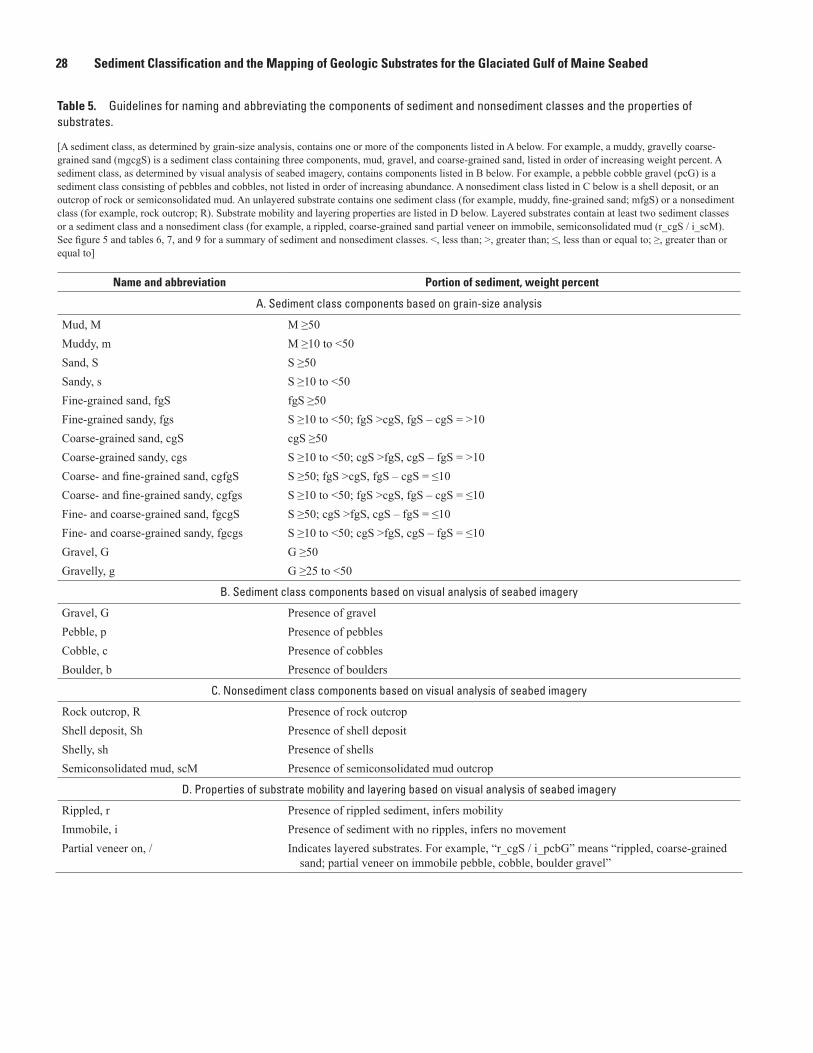
28 Sediment Classification and the Mapping of Geologic Substrates for the Glaciated Gulf of Maine Seabed
Table 5. Guidelines for naming and abbreviating the components of sediment and nonsediment classes and the properties of substrates.
[A sediment class, as determined by grain-size analysis, contains one or more of the components listed in A below. For example, a muddy, gravelly coarse-grained sand (mgcgS) is a sediment class containing three components, mud, gravel, and coarse-grained sand, listed in order of increasing weight percent. A sediment class, as determined by visual analysis of seabed imagery, contains components listed in B below. For example, a pebble cobble gravel (pcG) is a sediment class consisting of pebbles and cobbles, not listed in order of increasing abundance. A nonsediment class listed in C below is a shell deposit, or an outcrop of rock or semiconsolidated mud. An unlayered substrate contains one sediment class (for example, muddy, fine-grained sand; mfgS) or a nonsediment class (for example, rock outcrop; R). Substrate mobility and layering properties are listed in D below. Layered substrates contain at least two sediment classes or a sediment class and a nonsediment class (for example, a rippled, coarse-grained sand partial veneer on immobile, semiconsolidated mud (r_cgS / i_scM). See figure 5 and tables 6, 7, and 9 for a summary of sediment and nonsediment classes. <, less than; >, greater than; ≤, less than or equal to; ≥, greater than or equal to]
Name and abbreviation Portion of sediment, weight percent
A. Sediment class components based on grain-size analysis
Mud, M M ≥50Muddy, m M ≥10 to <50Sand, S S ≥50Sandy, s S ≥10 to <50Fine-grained sand, fgS fgS ≥50Fine-grained sandy, fgs S ≥10 to <50; fgS >cgS, fgS – cgS = >10Coarse-grained sand, cgS cgS ≥50Coarse-grained sandy, cgs S ≥10 to <50; cgS >fgS, cgS – fgS = >10Coarse- and fine-grained sand, cgfgS S ≥50; fgS >cgS, fgS – cgS = ≤10Coarse- and fine-grained sandy, cgfgs S ≥10 to <50; fgS >cgS, fgS – cgS = ≤10Fine- and coarse-grained sand, fgcgS S ≥50; cgS >fgS, cgS – fgS = ≤10Fine- and coarse-grained sandy, fgcgs S ≥10 to <50; cgS >fgS, cgS – fgS = ≤10Gravel, G G ≥50Gravelly, g G ≥25 to <50
B. Sediment class components based on visual analysis of seabed imagery
Gravel, G Presence of gravelPebble, p Presence of pebblesCobble, c Presence of cobblesBoulder, b Presence of boulders
C. Nonsediment class components based on visual analysis of seabed imagery
Rock outcrop, R Presence of rock outcropShell deposit, Sh Presence of shell depositShelly, sh Presence of shellsSemiconsolidated mud, scM Presence of semiconsolidated mud outcrop
D. Properties of substrate mobility and layering based on visual analysis of seabed imagery
Rippled, r Presence of rippled sediment, infers mobilityImmobile, i Presence of sediment with no ripples, infers no movementPartial veneer on, / Indicates layered substrates. For example, “r_cgS / i_pcbG” means “rippled, coarse-grained
sand; partial veneer on immobile pebble, cobble, boulder gravel”

Sediment-Classification-Related Tables and Seabed Photographs 29Ta
ble
6.
Clas
sific
atio
n of
nat
ural
ly o
ccur
ring
sedi
men
ts (s
edim
ent c
lass
es) b
ased
on
grai
n-si
ze a
naly
sis.
—Co
ntin
ued
[Crit
erio
n: m
ud o
r san
d or
gra
vel i
s ≥50
wei
ght p
erce
nt o
f the
sedi
men
t. A
ggre
gate
s and
com
posi
te g
rade
s are
list
ed in
ord
er o
f inc
reas
ing
wei
ght p
erce
nt. W
here
sand
is ≥
10 w
eigh
t per
cent
and
fine
-gra
ined
sa
nd a
nd c
oars
e-gr
aine
d sa
nd d
iffer
by
≤10
wei
ght p
erce
nt, t
he le
sser
of t
he tw
o is
list
ed fi
rst i
n th
e cl
ass n
ame,
for e
xam
ple,
mcg
fgS
is m
uddy
, coa
rse-
and
fine
-gra
ined
sand
, whe
re c
oars
e-gr
aine
d sa
nd is
less
th
an fi
ne-g
rain
ed sa
nd (s
edim
ent c
lass
7c)
. Whe
re sa
nd is
≥10
wei
ght p
erce
nt, a
nd fi
ne-g
rain
ed a
nd c
oars
e-gr
aine
d sa
nd d
iffer
by
>10
wei
ght p
erce
nt, o
nly
the
grea
ter o
f the
two
is li
sted
in th
e cl
ass n
ame,
for
exam
ple,
mfg
S is
mud
dy, fi
ne-g
rain
ed sa
nd, w
here
fine
-gra
ined
sand
is g
reat
er th
an c
oars
e-gr
aine
d sa
nd b
y >1
0 w
eigh
t per
cent
(cla
ss 7
a). S
ee fi
gure
5 fo
r ter
nary
dia
gram
show
ing
sedi
men
t cla
sses
list
ed in
co
lum
ns 4
and
5. S
ee ta
ble
5 fo
r exp
lana
tion
of a
bbre
viat
ions
. No.
, Num
ber;
<, le
ss th
an; >
, gre
ater
than
; ≤, l
ess t
han
or e
qual
to; ≥
, gre
ater
than
or e
qual
to]
Sedi
men
t cla
ssifi
ed b
y m
ud, s
and,
and
gra
vel c
onte
ntSe
dim
ent c
lass
ified
by
mud
, fin
e- a
nd c
oars
e-gr
aine
d sa
nd, a
nd g
rave
l con
tent
Sedi
men
t com
posi
tion
in
wei
ght p
erce
nt o
f mud
, san
d,
and
grav
el a
ggre
gate
s
Sedi
men
t cla
ssSa
nd c
ompo
sitio
n in
wei
ght p
erce
nt
of fi
ne- a
nd c
oars
e-gr
aine
d sa
nd
com
posi
te g
rade
s
Sedi
men
t cla
ss
No.
Nam
eA
bbre
-vi
atio
nN
o.N
ame
Abb
re-
viat
ion
Mud
, M≥5
0
S<10
, G<2
51
Mud
MS
<10
1M
udM
S<10
, G≥2
52
Gra
velly
mud
gM2
Gra
velly
mud
gM
S≥10
, G<2
53
Sand
y m
udsM
fgS
> cg
Sfg
S –
cgS
=>1
0>1
03a
Fine
-gra
ined
sand
y m
udfg
sMcg
S >
fgS
cgS
– fg
S =
3bC
oars
e-gr
aine
d sa
ndy
mud
cgsM
fgS
> cg
Sfg
S –
cgS
=≤1
0≤1
03c
Coa
rse-
and
fine
-gra
ined
sand
y m
udcg
fgsM
cgS
> fg
Scg
S –
fgS
=3d
Fine
- and
coa
rse-
grai
ned
sand
y m
udfg
cgsM
S≥10
, G≥2
5S<
G4
Sand
y, g
rave
lly m
udsg
M
fgS
> cg
Sfg
S –
cgS
=>1
0>1
04a
Fine
-gra
ined
sand
y, g
rave
lly m
udfg
sgM
cgS
> fg
Scg
S –
fgS
=4b
Coa
rse-
grai
ned
sand
y, g
rave
lly m
udcg
sgM
fgS
> cg
Sfg
S –
cgS
=≤1
0≤1
04c
Coa
rse-
and
fine
-gra
ined
sand
y, g
rave
lly m
udcg
fgsg
Mcg
S >
fgS
cgS
– fg
S =
4dFi
ne- a
nd c
oars
e-gr
aine
d sa
ndy,
gra
velly
mud
fgcg
sgM
Sand
, S≥5
0
M<1
0, G
<25
5Sa
ndS
fgS
> cg
Sfg
S –
cgS
=>1
0>1
05a
Fine
-gra
ined
sand
fgS
cgS
> fg
Scg
S –
fgS
=5b
Coa
rse-
grai
ned
sand
cgS
fgS
> cg
Sfg
S –
cgS
=≤1
0≤1
05c
Coa
rse-
and
fine
-gra
ined
sand
cgfg
Scg
S >
fgS
cgS
– fg
S =
5dFi
ne- a
nd c
oars
e-gr
aine
d sa
ndfg
cgS
M<1
0, G
≥25
6G
rave
lly sa
ndgS
fgS
> cg
Sfg
S –
cgS
=>1
0>1
06a
Gra
velly
, fine
-gra
ined
sand
gfgS
cgS
> fg
Scg
S –
fgS
=6b
Gra
velly
, coa
rse-
grai
ned
sand
gcgS
fgS
> cg
Sfg
S –
cgS
=≤1
0≤1
06c
Gra
velly
, coa
rse-
and
fine
-gra
ined
sand
gcgf
gScg
S >
fgS
cgS
– fg
S =
6dG
rave
lly, fi
ne- a
nd c
oars
e-gr
aine
d sa
ndgf
gcgS
M≥1
0, G
<25
7M
uddy
sand
mS
fgS
> cg
Sfg
S –
cgS
=>1
0>1
07a
Mud
dy, fi
ne-g
rain
ed sa
ndm
fgS
cgS
> fg
Scg
S –
fgS
=7b
Mud
dy, c
oars
e-gr
aine
d sa
ndm
cgS
fgS
> cg
Sfg
S –
cgS
=≤1
0≤1
07c
Mud
dy, c
oars
e- a
nd fi
ne-g
rain
ed sa
ndm
cgfg
Scg
S >
fgS
cgS
– fg
S =
7dM
uddy
, fine
- and
coa
rse-
grai
ned
sand
mfg
cgS
M≥1
0, G
≥25
M<G
8M
uddy
, gra
velly
sand
mgS
fgS
> cg
Sfg
S –
cgS
=>1
0>1
08a
Mud
dy, g
rave
lly, fi
ne-g
rain
ed sa
ndm
gfgS
cgS
> fg
Scg
S –
fgS
=8b
Mud
dy, g
rave
lly, c
oars
e-gr
aine
d sa
ndm
gcgS
fgS
> cg
Sfg
S –
cgS
=≤1
0≤1
08c
Mud
dy, g
rave
lly, c
oars
e- a
nd fi
ne-g
rain
ed sa
ndm
gcgf
gScg
S >
fgS
cgS
– fg
S =
8dM
uddy
, gra
velly
, fine
- and
coa
rse-
grai
ned
sand
mgf
gcgS

30 Sediment Classification and the Mapping of Geologic Substrates for the Glaciated Gulf of Maine SeabedTa
ble
6.
Clas
sific
atio
n of
nat
ural
ly o
ccur
ring
sedi
men
ts (s
edim
ent c
lass
es) b
ased
on
grai
n-si
ze a
naly
sis.
—Co
ntin
ued
[Crit
erio
n: m
ud o
r san
d or
gra
vel i
s ≥50
wei
ght p
erce
nt o
f the
sedi
men
t. A
ggre
gate
s and
com
posi
te g
rade
s are
list
ed in
ord
er o
f inc
reas
ing
wei
ght p
erce
nt. W
here
sand
is ≥
10 w
eigh
t per
cent
and
fine
-gra
ined
sa
nd a
nd c
oars
e-gr
aine
d sa
nd d
iffer
by
≤10
wei
ght p
erce
nt, t
he le
sser
of t
he tw
o is
list
ed fi
rst i
n th
e cl
ass n
ame,
for e
xam
ple,
mcg
fgS
is m
uddy
, coa
rse-
and
fine
-gra
ined
sand
, whe
re c
oars
e-gr
aine
d sa
nd is
less
th
an fi
ne-g
rain
ed sa
nd (s
edim
ent c
lass
7c)
. Whe
re sa
nd is
≥10
wei
ght p
erce
nt, a
nd fi
ne-g
rain
ed a
nd c
oars
e-gr
aine
d sa
nd d
iffer
by
>10
wei
ght p
erce
nt, o
nly
the
grea
ter o
f the
two
is li
sted
in th
e cl
ass n
ame,
for
exam
ple,
mfg
S is
mud
dy, fi
ne-g
rain
ed sa
nd, w
here
fine
-gra
ined
sand
is g
reat
er th
an c
oars
e-gr
aine
d sa
nd b
y >1
0 w
eigh
t per
cent
(cla
ss 7
a). S
ee fi
gure
5 fo
r ter
nary
dia
gram
show
ing
sedi
men
t cla
sses
list
ed in
co
lum
ns 4
and
5. S
ee ta
ble
5 fo
r exp
lana
tion
of a
bbre
viat
ions
. No.
, Num
ber;
<, le
ss th
an; >
, gre
ater
than
; ≤, l
ess t
han
or e
qual
to; ≥
, gre
ater
than
or e
qual
to]
Sedi
men
t cla
ssifi
ed b
y m
ud, s
and,
and
gra
vel c
onte
ntSe
dim
ent c
lass
ified
by
mud
, fin
e- a
nd c
oars
e-gr
aine
d sa
nd, a
nd g
rave
l con
tent
Sedi
men
t com
posi
tion
in
wei
ght p
erce
nt o
f mud
, san
d,
and
grav
el a
ggre
gate
s
Sedi
men
t cla
ssSa
nd c
ompo
sitio
n in
wei
ght p
erce
nt
of fi
ne- a
nd c
oars
e-gr
aine
d sa
nd
com
posi
te g
rade
s
Sedi
men
t cla
ss
No.
Nam
eA
bbre
-vi
atio
nN
o.N
ame
Abb
re-
viat
ion
Gra
vel,
G≥5
0
M<1
0, S
<10
9G
rave
lG
S <1
09
Gra
vel
G
M<1
0, S
≥10
10Sa
ndy
grav
elsG
fgS
> cg
Sfg
S –
cgS
=>1
0>1
010
aFi
ne-g
rain
ed sa
ndy
grav
elfg
sGcg
S >
fgS
cgS
– fg
S =
10b
Coa
rse-
grai
ned
sand
y gr
avel
cgsG
fgS
> cg
Sfg
S –
cgS
=≤1
0≤1
010
cC
oars
e- a
nd fi
ne-g
rain
ed sa
ndy
grav
elcg
fgsG
cgS
> fg
Scg
S –
fgS
=10
dFi
ne- a
nd c
oars
e-gr
aine
d sa
ndy
grav
elfg
cgsG
M ≥
10, S
<10
11M
uddy
gra
vel
mG
S <1
011
Mud
dy g
rave
lm
G
M≥1
0, S
≥10
S<M
12Sa
ndy,
mud
dy g
rave
lsm
G
fgS
> cg
Sfg
S –
cgS
=>1
0>1
012
aFi
ne-g
rain
ed sa
ndy,
mud
dy g
rave
lfg
smG
cgS
> fg
Scg
S –
fgS
=12
bC
oars
e-gr
aine
d sa
ndy,
mud
dy g
rave
lcg
smG
fgS
> cg
Sfg
S –
cgS
=≤1
0≤1
012
cC
oars
e- a
nd fi
ne-g
rain
ed sa
ndy,
mud
dy g
rave
lcg
fgsm
Gcg
S >
fgS
cgS
– fg
S =
12d
Fine
- and
coa
rse-
grai
ned
sand
y, m
uddy
gra
vel
fgcg
smG
M≥1
0, S
≥10
M<S
13M
uddy
, san
dy g
rave
lm
sG
fgS
> cg
Sfg
S –
cgS
=>1
0>1
013
aM
uddy
, fine
-gra
ined
sand
y gr
avel
mfg
sGcg
S >
fgS
cgS
– fg
S =
13b
Mud
dy, c
oars
e-gr
aine
d sa
ndy
grav
elm
cgsG
fgS
> cg
Sfg
S –
cgS
=≤1
0≤1
013
cM
uddy
, coa
rse-
and
fine
-gra
ined
sand
y gr
avel
mcg
fgsG
cgS
> fg
Scg
S –
fgS
=13
dM
uddy
, fine
- and
coa
rse-
grai
ned
sand
y gr
avel
mfg
cgsG
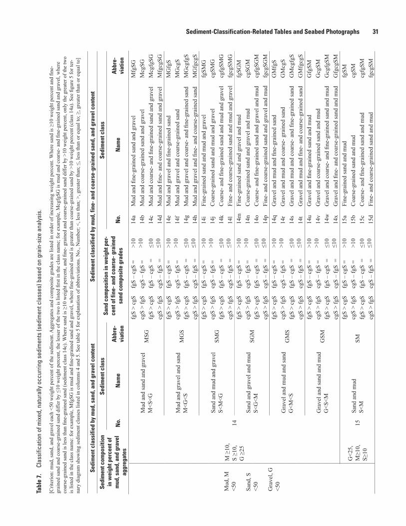
Sediment-Classification-Related Tables and Seabed Photographs 31Ta
ble
7.
Clas
sific
atio
n of
mix
ed, n
atur
ally
occ
urrin
g se
dim
ents
(sed
imen
t cla
sses
) bas
ed o
n gr
ain-
size
ana
lysi
s.—
Cont
inue
d
[Crit
erio
n: m
ud, s
and,
and
gra
vel e
ach
<50
wei
ght p
erce
nt o
f the
sedi
men
t. A
ggre
gate
s and
com
posi
te g
rade
s are
list
ed in
ord
er o
f inc
reas
ing
wei
ght p
erce
nt. W
here
sand
is ≥
10 w
eigh
t per
cent
and
fine
-gr
aine
d sa
nd a
nd c
oars
e-gr
aine
d sa
nd d
iffer
by
≤10
wei
ght p
erce
nt, t
he le
sser
of t
he tw
o is
list
ed fi
rst i
n th
e cl
ass n
ame;
for e
xam
ple,
Mcg
fgSG
is m
ud a
nd c
oars
e- a
nd fi
ne-g
rain
ed sa
nd a
nd g
rave
l, w
here
co
arse
-gra
ined
sand
is le
ss th
an fi
ne-g
rain
ed sa
nd (s
edim
ent c
lass
14c
). W
here
sand
is ≥
10 w
eigh
t per
cent
, and
fine
- gra
ined
and
coa
rse-
grai
ned
sand
diff
er b
y >1
0 w
eigh
t per
cent
, onl
y th
e gr
eate
r of t
he tw
o is
list
ed in
the
clas
s nam
e: fo
r exa
mpl
e, M
fgSG
is m
ud a
nd fi
ne-g
rain
ed sa
nd a
nd g
rave
l, w
here
fine
-gra
ined
sand
is g
reat
er th
an c
oars
e-gr
aine
d sa
nd b
y >1
0 w
eigh
t per
cent
(cla
ss 1
4a).
See
figur
e 5
for t
er-
nary
dia
gram
show
ing
sedi
men
t cla
sses
list
ed in
col
umns
4 a
nd 5
. See
tabl
e 5
for e
xpla
natio
n of
abb
revi
atio
ns. N
o., N
umbe
r; <,
less
than
; >, g
reat
er th
an; ≤
, les
s tha
n or
equ
al to
; ≥, g
reat
er th
an o
r equ
al to
]
Sedi
men
t cla
ssifi
ed b
y m
ud, s
and,
and
gra
vel c
onte
ntSe
dim
ent c
lass
ified
by
mud
, fin
e- a
nd c
oars
e-gr
aine
d sa
nd, a
nd g
rave
l con
tent
Sedi
men
t com
posi
tion
in w
eigh
t per
cent
of
mud
, san
d, a
nd g
rave
l ag
greg
ates
Sedi
men
t cla
ssSa
nd c
ompo
sitio
n in
wei
ght p
er-
cent
of f
ine-
and
coa
rse-
gra
ined
sa
nd c
ompo
site
gra
des
Sedi
men
t cla
ss
No.
Nam
eA
bbre
-vi
atio
nN
o.N
ame
Abb
re-
viat
ion
Mud
, M<5
0
Sand
, S<5
0
Gra
vel,
G<5
0
M ≥
10,
S ≥1
0,G
≥25
14
Mud
and
sand
and
gra
vel
M<S
<GM
SG
fgS
> cg
Sfg
S –
cgS
=>1
0>1
014
aM
ud a
nd fi
ne-g
rain
ed sa
nd a
nd g
rave
lM
fgSG
cgS
> fg
Scg
S –
fgS
=14
bM
ud a
nd c
oars
e-gr
aine
d sa
nd a
nd g
rave
lM
cgSG
fgS
> cg
Sfg
S –
cgS
=≤1
0≤1
014
cM
ud a
nd c
oars
e- a
nd fi
ne-g
rain
ed sa
nd a
nd g
rave
lM
cgfg
SGcg
S >
fgS
cgS
– fg
S =
14d
Mud
and
fine
- and
coa
rse-
grai
ned
sand
and
gra
vel
Mfg
cgSG
Mud
and
gra
vel a
nd sa
ndM
<G<S
MG
S
fgS
> cg
Sfg
S –
cgS
=>1
0>1
014
eM
ud a
nd g
rave
l and
fine
-gra
ined
sand
MG
fgS
cgS
> fg
Scg
S –
fgS
=14
fM
ud a
nd g
rave
l and
coa
rse-
grai
ned
sand
MG
cgS
fgS
> cg
Sfg
S –
cgS
=≤1
0≤1
014
gM
ud a
nd g
rave
l and
coa
rse-
and
fine
-gra
ined
sand
MG
cgfg
Scg
S >
fgS
cgS
– fg
S =
14h
Mud
and
gra
vel a
nd fi
ne- a
nd c
oars
e-gr
aine
d sa
ndM
Gfg
cgS
Sand
and
mud
and
gra
vel
S<M
<GSM
G
fgS
> cg
Sfg
S –
cgS
=>1
0>1
014
iFi
ne-g
rain
ed sa
nd a
nd m
ud a
nd g
rave
lfg
SMG
cgS
> fg
Scg
S –
fgS
=14
jC
oars
e-gr
aine
d sa
nd a
nd m
ud a
nd g
rave
lcg
SMG
fgS
> cg
Sfg
S –
cgS
=≤1
0≤1
014
kC
oars
e- a
nd fi
ne-g
rain
ed sa
nd a
nd m
ud a
nd g
rave
lcg
fgSM
Gcg
S >
fgS
cgS
– fg
S =
14l
Fine
- and
coa
rse-
grai
ned
sand
and
mud
and
gra
vel
fgcg
SMG
Sand
and
gra
vel a
nd m
udS<
G<M
SGM
fgS
> cg
Sfg
S –
cgS
=>1
0>1
014
mFi
ne-g
rain
ed sa
nd a
nd g
rave
l and
mud
fgSG
Mcg
S >
fgS
cgS
– fg
S =
14n
Coa
rse-
grai
ned
sand
and
gra
vel a
nd m
udcg
SGM
fgS
> cg
Sfg
S –
cgS
=≤1
0≤1
014
oC
oars
e- a
nd fi
ne-g
rain
ed sa
nd a
nd g
rave
l and
mud
cgfg
SGM
cgS
> fg
Scg
S –
fgS
=14
pFi
ne- a
nd c
oars
e-gr
aine
d sa
nd a
nd g
rave
l and
mud
fgcg
SGM
Gra
vel a
nd m
ud a
nd sa
ndG
<M<S
GM
S
fgS
> cg
Sfg
S –
cgS
=>1
0>1
014
qG
rave
l and
mud
and
fine
-gra
ined
sand
GM
fgS
cgS
> fg
Scg
S –
fgS
=14
rG
rave
l and
mud
and
coa
rse-
gra
ined
sand
GM
cgS
fgS
> cg
Sfg
S –
cgS
=≤1
0≤1
014
sG
rave
l and
mud
and
coa
rse-
and
fine
-gra
ined
sand
GM
cgfg
Scg
S >
fgS
cgS
– fg
S =
14t
Gra
vel a
nd m
ud a
nd fi
ne- a
nd c
oars
e-gr
aine
d sa
ndG
Mfg
cgS
Gra
vel a
nd sa
nd a
nd m
udG
<S<M
GSM
fgS
> cg
Sfg
S –
cgS
=>1
0>1
014
uG
rave
l and
fine
-gra
ined
sand
and
mud
Gfg
SMcg
S >
fgS
cgS
– fg
S =
14v
Gra
vel a
nd c
oars
e-gr
aine
d sa
nd a
nd m
udG
cgSM
fgS
> cg
Sfg
S –
cgS
=≤1
0≤1
014
wG
rave
l and
coa
rse-
and
fine
-gra
ined
sand
and
mud
Gcg
fgSM
cgS
> fg
Scg
S –
fgS
=14
xG
rave
l and
fine
- and
coa
rse-
grai
ned
sand
and
mud
Gfg
cgSM
G<2
5,M
≥10,
S≥10
15Sa
nd a
nd m
udS<
MSM
fgS
> cg
Sfg
S –
cgS
=>1
015
aFi
ne-g
rain
ed sa
nd a
nd m
udfg
SMcg
S >
fgS
cgS
– fg
S =
>10
15b
Coa
rse-
grai
ned
sand
and
mud
cgSM
fgS
> cg
Sfg
S –
cgS
=≤1
0≤1
015
cC
oars
e- a
nd fi
ne-g
rain
ed sa
nd a
nd m
udcg
fgSM
cgS
> fg
Scg
S –
fgS
=15
dFi
ne- a
nd c
oars
e-gr
aine
d sa
nd a
nd m
udfg
cgSM

32 Sediment Classification and the Mapping of Geologic Substrates for the Glaciated Gulf of Maine SeabedTa
ble
7.
Clas
sific
atio
n of
mix
ed, n
atur
ally
occ
urrin
g se
dim
ents
(sed
imen
t cla
sses
) bas
ed o
n gr
ain-
size
ana
lysi
s.—
Cont
inue
d
[Crit
erio
n: m
ud, s
and,
and
gra
vel e
ach
<50
wei
ght p
erce
nt o
f the
sedi
men
t. A
ggre
gate
s and
com
posi
te g
rade
s are
list
ed in
ord
er o
f inc
reas
ing
wei
ght p
erce
nt. W
here
sand
is ≥
10 w
eigh
t per
cent
and
fine
-gr
aine
d sa
nd a
nd c
oars
e-gr
aine
d sa
nd d
iffer
by
≤10
wei
ght p
erce
nt, t
he le
sser
of t
he tw
o is
list
ed fi
rst i
n th
e cl
ass n
ame;
for e
xam
ple,
Mcg
fgSG
is m
ud a
nd c
oars
e- a
nd fi
ne-g
rain
ed sa
nd a
nd g
rave
l, w
here
co
arse
-gra
ined
sand
is le
ss th
an fi
ne-g
rain
ed sa
nd (s
edim
ent c
lass
14c
). W
here
sand
is ≥
10 w
eigh
t per
cent
, and
fine
- gra
ined
and
coa
rse-
grai
ned
sand
diff
er b
y >1
0 w
eigh
t per
cent
, onl
y th
e gr
eate
r of t
he tw
o is
list
ed in
the
clas
s nam
e: fo
r exa
mpl
e, M
fgSG
is m
ud a
nd fi
ne-g
rain
ed sa
nd a
nd g
rave
l, w
here
fine
-gra
ined
sand
is g
reat
er th
an c
oars
e-gr
aine
d sa
nd b
y >1
0 w
eigh
t per
cent
(cla
ss 1
4a).
See
figur
e 5
for t
er-
nary
dia
gram
show
ing
sedi
men
t cla
sses
list
ed in
col
umns
4 a
nd 5
. See
tabl
e 5
for e
xpla
natio
n of
abb
revi
atio
ns. N
o., N
umbe
r; <,
less
than
; >, g
reat
er th
an; ≤
, les
s tha
n or
equ
al to
; ≥, g
reat
er th
an o
r equ
al to
]
Sedi
men
t cla
ssifi
ed b
y m
ud, s
and,
and
gra
vel c
onte
ntSe
dim
ent c
lass
ified
by
mud
, fin
e- a
nd c
oars
e-gr
aine
d sa
nd, a
nd g
rave
l con
tent
Sedi
men
t com
posi
tion
in w
eigh
t per
cent
of
mud
, san
d, a
nd g
rave
l ag
greg
ates
Sedi
men
t cla
ssSa
nd c
ompo
sitio
n in
wei
ght p
er-
cent
of f
ine-
and
coa
rse-
gra
ined
sa
nd c
ompo
site
gra
des
Sedi
men
t cla
ss
No.
Nam
eA
bbre
-vi
atio
nN
o.N
ame
Abb
re-
viat
ion
Mud
, M<5
0
Sand
, S<5
0
Gra
vel,
G<5
0
G<2
5,M
≥10,
S≥10
16M
ud a
nd sa
ndM
<SM
S
fgS
> cg
Sfg
S –
cgS
=>1
016
aM
ud a
nd fi
ne-g
rain
ed sa
ndM
fgS
cgS
> fg
Scg
S –
fgS
=>1
016
bM
ud a
nd c
oars
e-gr
aine
d sa
ndM
cgS
fgS
> cg
Sfg
S –
cgS
=≤1
0≤1
016
cM
ud a
nd c
oars
e- a
nd fi
ne-g
rain
ed sa
ndM
cgfg
Scg
S >
fgS
cgS
– fg
S =
16d
Mud
and
fine
- and
coa
rse-
grai
ned
sand
Mfg
cgS
M<1
0,S≥
10,
G≥2
517
Gra
vel a
nd sa
ndG
<SG
S
fgS
> cg
Sfg
S –
cgS
=>1
0>1
017
aG
rave
l and
fine
-gra
ined
sand
Gfg
Scg
S >
fgS
cgS
– fg
S =
17b
Gra
vel a
nd c
oars
e-gr
aine
d sa
ndG
cgS
fgS
> cg
Sfg
S –
cgS
=≤1
0≤1
017
cG
rave
l and
coa
rse-
and
fine
-gra
ined
sand
Gcg
fgS
cgS
> fg
Scg
S –
fgS
=17
dG
rave
l and
fine
- and
coa
rse-
grai
ned
sand
Gfg
cgS
M<1
0,S≥
10,
G≥2
518
Sand
and
gra
vel
S<G
SG
fgS
> cg
Sfg
S –
cgS
=>1
0>1
018
aFi
ne-g
rain
ed sa
nd a
nd g
rave
lfg
SGcg
S >
fgS
cgS
– fg
S =
18b
Coa
rse-
grai
ned
sand
and
gra
vel
cgSG
fgS
> cg
Sfg
S –
cgS
=≤1
0≤1
018
cC
oars
e- a
nd fi
ne-g
rain
ed sa
nd a
nd g
rave
lcg
fgSG
cgS
> fg
Scg
S –
fgS
=18
dFi
ne- a
nd c
oars
e-gr
aine
d sa
nd a
nd g
rave
lfg
cgSG
S<10
,M
≥10,
G≥2
519
Gra
vel a
nd m
udG
<MG
M
S<10
19G
rave
l and
mud
GM
S<10
,M
≥10,
G≥2
520
Mud
and
gra
vel
M<G
MG
20M
ud a
nd g
rave
lM
G

Sediment-Classification-Related Tables and Seabed Photographs 33Ta
ble
8.
Prop
ertie
s of
map
ped
geol
ogic
sub
stra
tes
in q
uadr
angl
e 6
of th
e St
ellw
agen
Ban
k N
atio
nal M
arin
e Sa
nctu
ary
regi
on.
[Com
posi
te g
rade
s are
list
ed in
ital
ics.
Text
ural
pro
perti
es fo
r unl
ayer
ed su
bstra
tes (
A1,
A2,
E, G
1, G
2) a
re b
ased
on
grai
n-si
ze a
naly
sis.
For l
ayer
ed su
bstra
tes (
B, D
1, D
2, F
), te
xtur
al p
rope
rties
are
bas
ed o
n gr
ain-
size
ana
lysi
s of t
he u
pper
subs
trate
that
par
tially
ven
eers
the
low
er su
bstra
te o
f com
bina
tions
of p
ebbl
e, c
obbl
e, a
nd b
ould
er g
rave
l. Th
e un
derly
ing
grav
el is
iden
tified
bas
ed o
n vi
deo
imag
ery.
Sub
stra
te
C is
not
list
ed a
s it c
onsi
sts o
f bou
lder
ridg
es id
entifi
ed b
y se
abed
topo
grap
hy a
nd v
isua
l ins
pect
ion
usin
g vi
deo
imag
ery.
Wei
ght p
erce
nt (w
t pct
) val
ues m
ay n
ot a
dd to
100
ow
ing
to ro
undi
ng; <
1 m
eans
≤0.
5 w
eigh
t per
cent
. A sa
nd o
r gra
vel g
rade
or m
ud (>
4 ph
i) is
term
ed “
sign
ifica
nt”
in a
subs
trate
if it
s mea
n w
eigh
t per
cent
for a
ll sa
mpl
es o
f a su
bstra
te is
≥10
. Sed
imen
t com
pone
nts o
f an
unla
yere
d su
bstra
te
(or t
he u
pper
subs
trate
of a
laye
red
subs
trate
) are
list
ed in
ord
er o
f inc
reas
ing
wei
ght p
erce
nt in
the
sedi
men
t cla
ss n
ame.
Sed
imen
t com
pone
nts o
f the
low
er su
bstra
te in
dica
te p
rese
nce/
abse
nce,
and
are
not
lis
ted
in o
rder
of i
ncre
asin
g ar
eal c
over
age
in th
e se
dim
ent c
lass
nam
e. S
ubst
rate
nam
es c
ombi
ne a
uni
que
sym
bol,
a m
obili
ty te
rm, a
sedi
men
t cla
ss te
rm d
eriv
ed fr
om g
rain
-siz
e an
alys
is, a
laye
ring
term
(/) i
f su
bstra
te la
yers
are
pre
sent
, and
a se
dim
ent c
lass
term
des
crib
ing
the
low
er su
bstra
te b
ased
on
vide
o an
d ph
oto
imag
ery.
fgS,
fine
-gra
ined
sand
(3 a
nd 4
phi
com
bine
d); c
gS, c
oars
e-gr
aine
d sa
nd (0
, 1, a
nd 2
phi
co
mbi
ned)
; G1,
Gra
vel 1 (
-1 a
nd -2
phi
com
bine
d); G
2, G
rave
l 2 (-3
, -4,
and
-5 p
hi c
ombi
ned)
. No.
, num
ber o
f sam
ples
; m, m
eter
; min
, min
imum
; max
, max
imum
; mm
, mill
imet
er; <
, les
s tha
n; >
, gre
ater
than
; ≥,
gre
ater
than
or e
qual
to; ~
, app
roxi
mat
ely]
Geo
logi
c su
bstr
ate
sym
bol
No.
Sam
ple
wat
er d
epth
ra
nge;
mea
n (m
)
Sign
ifica
nt s
edim
ent g
rade
sW
eigh
t per
cent
of a
ggre
gate
s an
d co
mpo
site
gra
des
th
at o
ccur
in th
e su
bstr
ate
Subs
trat
e na
me
sym
bol
mob
ility
_ se
dim
ent c
lass
Subs
trat
e na
me
tran
slat
ion
Mea
n w
eigh
t pe
rcen
t,
phi (φ)
gra
des;
to
tal w
t pct
Gra
in d
iam
eter
m
in–m
ax; m
ax
diffe
renc
e (m
m)
Sam
-pl
esM
udfg
Scg
SSa
ndG
1G
2G
rave
l
A1
128
30–5
641
2φ (1
4), 1
φ (4
5),
0φ (2
8)87
0.25
–<2.
0~1
.75
Ran
geM
ean
0–1
<1
<1–
15 350
–98
8852
–99
90<
1–26 8
0–21 1
<1–4
79
A1
r_cg
SA
1—rip
pled
, coa
rse-
grai
ned
sand
A2
2653
–77
623φ
(10)
, 2φ
(19)
,1φ
(35)
, 0φ
(19)
83
0.12
5–<2
.0~1
.875
Ran
geM
ean
<1–
11
2–37 11
32–9
372
44–9
883
1–36 11
0–35 5
1–55 16
A2
i_cg
SA
2—im
mob
ile, c
oars
e-gr
aine
d sa
nd
B22
36–5
848
2φ (1
9), 1
φ (4
0),
0φ (2
7)86
0.25
–<2.
0~1
.75
Ran
geM
ean
0–1
<1
2–21 5
65–9
786
78–9
992
<1–
20 70–
8 1<1
–22
8B
r_cg
S/i_
cbG
B—
rippl
ed, c
oars
e-gr
aine
d sa
nd;
parti
al v
enee
r on
imm
obile
co
bble
, bou
lder
gra
vel
D1
2850
–83
613φ
(14)
, 2φ
(15)
,1φ
(11)
, -3φ
(13)
,-4
φ (1
3)66
0.12
5–<3
2~3
1.87
5R
ange
Mea
n1–
9 43–
46 167–
64 3415
–92
502–
31 113–
75 345–
81 45D
1 i_
gcgS
/pcb
GD
1—im
mob
ile, g
rave
lly, c
oars
e-gr
aine
d sa
nd; p
artia
l ven
eer o
n pe
bble
, cob
ble,
bou
lder
gra
vel
D2
1587
–105
94>4
φ (1
2), 3
φ (1
5),
2φ (2
1), 1
φ (2
3),
0φ (1
0)81
>0–<
2.0
~2R
ange
Mea
n8–
22 1211
–42
2234
–65
5555
–89
761–
14 80–
25 43–
34 12D
2 i_
mcg
S/pc
bGD
2—im
mob
ile, m
uddy
, coa
rse-
grai
ned
sand
; par
tial v
enee
r on
pebb
le, c
obbl
e, b
ould
er g
rave
l
E31
66–1
2280
3φ (1
6), 2
φ (2
6),
1φ (2
8), 0
φ (1
0)80
0.12
5–<2
.0~1
.875
Ran
geM
ean
2–10 4
3–48 18
24–8
764
38–9
882
0–28 9
0–26 5
0–53 14
E i_
cgS
E—im
mob
ile, c
oars
e-gr
aine
d sa
nd
F21
90–1
4811
13φ
(17)
, 2φ
(16)
,1φ
(17)
, 0φ
(11)
61
0.12
5–<2
.0~1
.875
Ran
geM
ean
5–14 9
8–54 25
20–6
544
39–9
169
0–27 13
0–32 9
0–54 22
F i_
cgS/
pcbG
F—im
mob
ile, c
oars
e-gr
aine
d sa
nd; p
artia
l ven
eer o
n pe
bble
, co
bble
, bou
lder
gra
vel
G1
3985
–171
113
>4φ
(10)
, 4φ
(29)
,3φ
(49)
88
>0–<
0.25
0~0
.250
Ran
geM
ean
2–18 10
44–9
478
0–39 10
80–9
788
<1–
51
1–7 1
0–8 1
G1
i_m
fgS
G1—
imm
obile
, mud
dy, fi
ne-
grai
ned
sand
G2
912
5–18
514
5>4
φ (2
3), 4
φ (5
8),
3φ (1
9)10
0
>0–<
0.25
0~0
.250
Ran
geM
ean
19–2
923
70–8
077
0–2 1
71–8
177
0–0 1
0–0 0
0–0 1
G2
i_m
fgS
G2—
imm
obile
, mud
dy, fi
ne-
grai
ned
sand
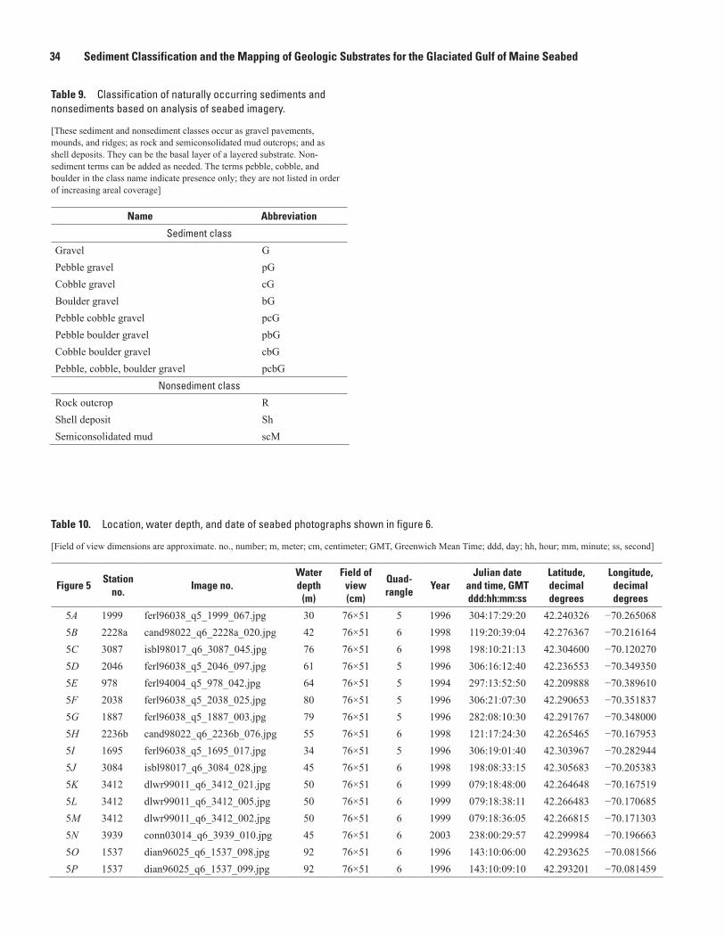
34 Sediment Classification and the Mapping of Geologic Substrates for the Glaciated Gulf of Maine Seabed
Table 9. Classification of naturally occurring sediments and nonsediments based on analysis of seabed imagery.
[These sediment and nonsediment classes occur as gravel pavements, mounds, and ridges; as rock and semiconsolidated mud outcrops; and as shell deposits. They can be the basal layer of a layered substrate. Non-sediment terms can be added as needed. The terms pebble, cobble, and boulder in the class name indicate presence only; they are not listed in order of increasing areal coverage]
Name Abbreviation
Sediment class
Gravel GPebble gravel pGCobble gravel cGBoulder gravel bGPebble cobble gravel pcGPebble boulder gravel pbGCobble boulder gravel cbGPebble, cobble, boulder gravel pcbG
Nonsediment class
Rock outcrop RShell deposit ShSemiconsolidated mud scM
Table 10. Location, water depth, and date of seabed photographs shown in figure 6.
[Field of view dimensions are approximate. no., number; m, meter; cm, centimeter; GMT, Greenwich Mean Time; ddd, day; hh, hour; mm, minute; ss, second]
Figure 5Station
no.Image no.
Water depth
(m)
Field of view (cm)
Quad-rangle
YearJulian date
and time, GMT ddd:hh:mm:ss
Latitude, decimal degrees
Longitude, decimal degrees
5A 1999 ferl96038_q5_1999_067.jpg 30 76×51 5 1996 304:17:29:20 42.240326 −70.2650685B 2228a cand98022_q6_2228a_020.jpg 42 76×51 6 1998 119:20:39:04 42.276367 −70.2161645C 3087 isbl98017_q6_3087_045.jpg 76 76×51 6 1998 198:10:21:13 42.304600 −70.1202705D 2046 ferl96038_q5_2046_097.jpg 61 76×51 5 1996 306:16:12:40 42.236553 −70.3493505E 978 ferl94004_q5_978_042.jpg 64 76×51 5 1994 297:13:52:50 42.209888 −70.3896105F 2038 ferl96038_q5_2038_025.jpg 80 76×51 5 1996 306:21:07:30 42.290653 −70.3518375G 1887 ferl96038_q5_1887_003.jpg 79 76×51 5 1996 282:08:10:30 42.291767 −70.3480005H 2236b cand98022_q6_2236b_076.jpg 55 76×51 6 1998 121:17:24:30 42.265465 −70.1679535I 1695 ferl96038_q5_1695_017.jpg 34 76×51 5 1996 306:19:01:40 42.303967 −70.2829445J 3084 isbl98017_q6_3084_028.jpg 45 76×51 6 1998 198:08:33:15 42.305683 −70.2053835K 3412 dlwr99011_q6_3412_021.jpg 50 76×51 6 1999 079:18:48:00 42.264648 −70.1675195L 3412 dlwr99011_q6_3412_005.jpg 50 76×51 6 1999 079:18:38:11 42.266483 −70.1706855M 3412 dlwr99011_q6_3412_002.jpg 50 76×51 6 1999 079:18:36:05 42.266815 −70.1713035N 3939 conn03014_q6_3939_010.jpg 45 76×51 6 2003 238:00:29:57 42.299984 −70.1966635O 1537 dian96025_q6_1537_098.jpg 92 76×51 6 1996 143:10:06:00 42.293625 −70.0815665P 1537 dian96025_q6_1537_099.jpg 92 76×51 6 1996 143:10:09:10 42.293201 −70.081459
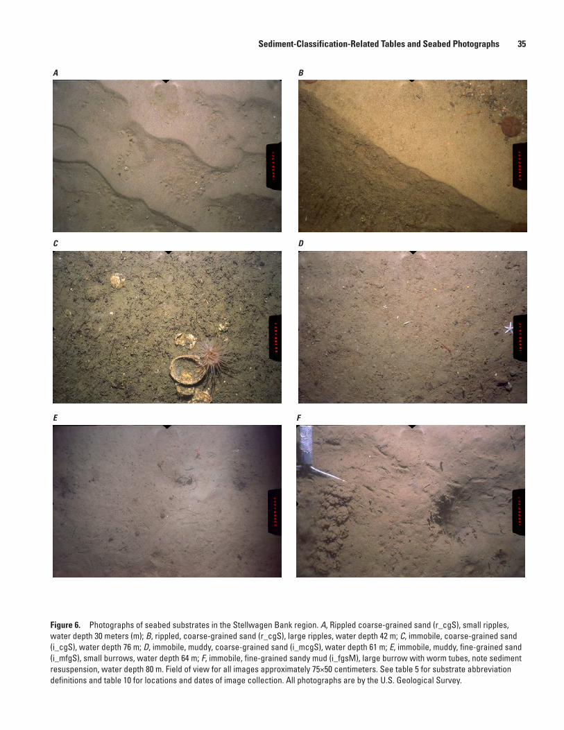
Sediment-Classification-Related Tables and Seabed Photographs 35
A B
C D
E F
Figure 6. Photographs of seabed substrates in the Stellwagen Bank region. A, Rippled coarse-grained sand (r_cgS), small ripples, water depth 30 meters (m); B, rippled, coarse-grained sand (r_cgS), large ripples, water depth 42 m; C, immobile, coarse-grained sand (i_cgS), water depth 76 m; D, immobile, muddy, coarse-grained sand (i_mcgS), water depth 61 m; E, immobile, muddy, fine-grained sand (i_mfgS), small burrows, water depth 64 m; F, immobile, fine-grained sandy mud (i_fgsM), large burrow with worm tubes, note sediment resuspension, water depth 80 m. Field of view for all images approximately 75×50 centimeters. See table 5 for substrate abbreviation definitions and table 10 for locations and dates of image collection. All photographs are by the U.S. Geological Survey.

36 Sediment Classification and the Mapping of Geologic Substrates for the Glaciated Gulf of Maine Seabed
G H
I J
K L
Figure 6. Photographs of seabed substrates in the Stellwagen Bank region. G, Immobile, fine-grained sandy mud (i_fgsM, burrow and cerianthid burrowing anemones, water depth 79 meters (m); H, immobile, pebble cobble gravel (i_pcG), water depth 55 m; I, layered substrate, rippled, coarse-grained sand partial veneer on immobile pebble, cobble, boulder gravel (r_cgS / i_pcbG), water depth 34 m; J, layered substrate, rippled, coarse-grained sand partial veneer on immobile pebble, cobble, boulder gravel (r_cgS / i_pcbG), water depth 45 m; K, layered substrate, immobile, coarse-grained sand, partial veneer on pebble gravel (i_cgS / pG), first of three images that show increasing veneer of coarse-grained sand along the same video drift (see figs. 5L, M), water depth 50 m; L, layered substrate, immobile, coarse-grained sand, partial veneer on pebble gravel (i_cgS / pG), second of three images that show increasing veneer of coarse-grained sand along the same video drift (see figs. 5K, M), water depth 50 m—Continued

Sediment-Classification-Related Tables and Seabed Photographs 37
M N
O P
Figure 6. Photographs of seabed substrates in the Stellwagen Bank region. M, Layered substrate, immobile, coarse-grained sand, partial veneer on pebble gravel (i_cgS / pG), third of three images that show increasing veneer of coarse-grained sand along the same video drift (see figs. 6K and L), water depth 50 meters (m); N, layered substrate, immobile, coarse-grained sand, partial veneer on semiconsolidated mud (i_cgS / scM), burrows in semiconsolidated mud partially filled with coarse-grained sand, water depth 45 m; O, layered substrate, immobile, muddy, coarse-grained sand, partial veneer on pebble, cobble, boulder gravel (i_mcgS / pcbG), brachiopods attach to hard substrate, water depth 92 m; P, layered substrate, immobile, muddy, coarse-grained sand, partial veneer on pebble, cobble, boulder gravel (i_mcgS / pcbG), brachiopods attach to hard substrate, water depth 92 m.—Continued


For more information about this report, contact:Director, Woods Hole Coastal and Marine Science CenterU.S. Geological Survey384 Woods Hole RoadQuissett CampusWoods Hole, MA 02543–[email protected](508) 548–8700 or (508) 457–2200or visit our website athttps://woodshole.er.usgs.gov
Publishing support provided by the Pembroke and West Trenton Publishing Service Centers

Valentine—Sedim
ent Classification and the Mapping of G
eologic Substrates for the Glaciated G
ulf of Maine Seabed—
Scientific Investigations Report 2019–5073
ISSN 2328-0328 (online)https://doi.org/10.3133/sir20195073