Counting in Anonymous Dynamic Networks: An

Experimental Perspective

Abstract

To implement high level abstractions, counting is undoubtedly a fundamental

problem for all of distributed system, because it represents a basic component. In

anonymous dynamic networks, because all nodes have no identity and a priori knowledge

of the network, counting is vitally important. Based on two leader-based algorithms,

namely ANoK and ALCO, these two algorithms count the exact number of nodes using

the notion of energy transfer. However, there is a limitation, ANoK just makes sure the

leader can get the number of processes but it is unable to recognize when this happens.

This paper will describe and analyze a new algorithm A*Nok which asks the leader to

make a prediction about when it produces the current count, then we use an experiment to

evaluate both algorithms. In addition, this paper will provide a new algorithm A*LCO to

accelerate the convergence time as well.

Acknowledgements

After four months of hard work, this project finally came to fruition. Although I had

encountered many problems, I overcame all kinds of difficulties by many people’s help. First of

all, I give sincerest gratitude to my supervisor, Evangelos Kranakis, he has supported me

throughout my project and help me to find idea to work in my way. If I did not get his support

and encouragement, then this paper would not have been finished or even started. I do not think I

can get a nicer supervisor than him and do not think I can get better help than what I already got.

There were a lot of teachers and students provided help to me. When I got problems, they

tried to lead me to find answers. When I had no idea what should I do, then they will help me

figure out what I can do next. They are always with me, give me encourage, give me supports, let

me can finish this project. Now, I want to give my heartfelt thanks to you, and I also have to say

sorry I had always disturb yours in the last four months.

Moreover, thanks for the Department of Computer Science, which has given the

equipment and support for all I have needed to start and finish my project.

Finally, I want to give my sincere regards to my family for their full supporting to me

throughout all my studies at Carleton University, thus let me only focus on my studying, do not

need to worry about any life problem.

1. Introduction

In the 21st century, because of the rapidly development of computer technology,

the word “network” is being used more and more often in people’s life. The network

maybe used as small as entertainment, shopping, studying or maybe used personal

business, international business, even some government and martial. I may predict the

network will cover our life anywhere in the near future. Now, let us turn our attention

back to today. With the development, of time, computer and network technology is

progressing with each passing day. In particular cause for concern, the distributed

computing systems are switching from static to more and more dynamic. The

computation’s relatively stable and traditional static models will no longer suit for the now

established and fast emerging technologies of information. You may notice that,

nowadays, there are more and more new mobile computing devices integrate successfully

into people’s work and life. Most of them can provide the capabilities of communication,

sensing, mobility and so on. Even the internet has gradually shifted from wireless

internet to wireless mobile internet. Networked use sensors and mobile devices to

produce data exchanges between real world and modern and traditional networks,

includes information, communication and social networks. Thus, such a kind of hyper-

connected dynamic environments brought a chance to us to solve what the old static

distributed system cannot capture. There was a good example we can see:

A highly dynamic, less infrastructure network - Delay-tolerant networks (DNT),

which is also known as Disruption Tolerant Networks. This DTN is used to deal with the

problem in heterogeneous networks, this kind of network may not always have the continuous

network connectivity. Under some certain network environment, network will become

disconnected, so that the communication routs of message cannot guarantee it is an end-

to-end communication routes. However, the DNT provide a basic characteristic is at any

instant there can be no end-to-end communication routes. The completely predictable

mobility can change a completely unpredictable mobility. The research of DNT will

bring a powerfully theory and technology’s support to the messaging interactions in the

domain of military flights, aerospace, disaster recovery, emergency rescue and so on.

Unfortunately, the research of dynamic communication networks is still at a

beginning stage. In the field of distributed computing still have lots of work needs to be

done, includes changes and failures in the topology that are slow and even stabilize

ultimately. Actually, the topological changed very slowly that is considered it is

inappropriate for inferring about dynamic networks. Othon [3] stated that “even graph

theoretic techniques need to be revisited: the suitable graph model is now that of a

dynamic graph in which each edge has an associated set of time labels indicating

availability times. Even fundamental properties of classical graphs do not carry over to

their temporal counterparts.” (Othon, Ioannis, & Paul 2012)

At present, from a social aspect, a critical issue in designing dynamic network is

security and trust. This new form network has many special features, such as dynamic

changing topology, open communication medium, limited node, channel resource and so

on. However, those features more like a two-edged sword, which has its good and bad

points at the same time. In designing such a hyper-connected dynamic infrastructure, it

makes information become more possible be monitor and intercepted. For example,

followed an increasing number of people use social networking application, the problem

of privacy invasion and the inappropriate transfer of personal information became

especially serious. The problems brought a series of inconvenience, even danger to

people’s life. Moreover, some special departments appeared to have a higher and higher

security requirement to wireless mobile internet, includes military, government, and

defense department. Therefore, because of those security threats, we can see that we need

to figure out a way to solve this problem as soon as possible, this research field also has

become a hotspot laid before us. At this time, there was a kind of anonymous network

came into people’s view.

In fact, networks is now struggling for dealing with attacker’s tracking and

monitoring online. Such as data confidentiality and integrity, identification, information

security and entity authentication, all of those aspects need to be considered instead of

only focus on elective targeting, data aggregating and profiling. In order to solve this

problem, mobile networks have to provide anonymous service to conceal the identity of

the mobile node, so anonymous service plays a significant role in the mobile service. This

is what we called anonymity of the artifacts. Although, traditional encryption technology

would also make some protection to data privacy and security, integrity and identity in

the mobile network, but attackers can still get the source, destination, quantity, and some

implication of the message. Moreover, they even can deduce the confidential information

of node identity, location and so on by analyses the transfer mode and the header

information of messages, such as source addresses and destination addresses, length of

messages. After that, based on that information they can launch targeted attacks.

However, the technology of anonymous can hide the communication relationship in

communication streaming through a certain technique, such that attacker cannot know the

relationship or identity of communicators. Also, the strategy of dynamic anonymous

network in wireless mobile internet can well adapt to the complicate network topology

structure, lower system overhead and improve efficient.

In this project, I will explore a basic problem in the dynamic anonymous network

– Counting. Counting nodes' number in the network but without any prior information of

the node or the network state, in other words, nodes do not know the size of the network

is what I want to present in this work. Counting is the most basic and important problem

in the distributed computation, which is a central part in the management and control of

network. In the future, networks should be extremely dynamic: after received message

the connected artifacts become immediately unreachable. For now, the current theoretical

models of dynamic networks, their topology is usually changing arbitrarily round to

round. The edge represents communication is changed at each round by an opponent

among hype-connected artifacts, so that modify the edges is constricted as the network is

always connected. Also some edges are random distributed with a certain properties.

Under these assumptions taken for granted, based on the theoretical results we can create

a robust, scalable and that terminate protocol for distributed task.

Right now, we need to forget the assumptions that we see from the previous

theoretical models:

1) There is not any prior knowledge about networks, nodes do not known

the size n of the network, and other metric.

2) Nodes are initially identical, which means they have no unique

identities and execute same programs. Except for a leader is not

introduced, nodes execute same programs in symmetric networks that

cannot be count.

3) The network does not have to be connected at any time.

I trust the desire mode of operation is work well for the future hype-connected

environments, and privacy also be considered in this model. Based on these conditions,

we present a distributed algorithm was called A*Nok, and to avoid looking for the size of

the anonymous network I used the termination heuristic. This algorithm is based on a no

knowledge algorithm ANok that was established in another paper [2]. I are going to use an

energy-transfer technique to find what exact number of nodes is in the anonymous

network.

In order to examine the performance of those two algorithm A*Nok and ANok, I use

an experimental approach to do so. Also, I try to use an algorithm ALOC to compare with

A*Nok. Then I change the ALOC to let it work under a more generic mode of operation,

called A*LOC. I use different random evolving graph models to test the algorithm’s error

rate and efficiency for terminating the computation. I also use the periodically

disconnected networks as the artifacts duty-cycle.

Under densely connected anonymous networks, algorithm A*NoK terminate always

correctly. For the network experience regular partitions, A*NoK can predict the accuracy of

the size varies corresponding to the degree of disconnection of the network. The accuracy

in counting decreased when the periods of network disconnections get longer. Thus, we

can conclude that the algorithm A*NoK can predicate “does the network contain more than

N nodes?” in a certain rounds, and it is lesser than what we see from [2] used in

algorithm ANoK.

2 Preliminaries

Energy – Transfer Technique. A technique used a simple method of energy transfer to

count the number of nodes in the networks with a constantly dynamic environment and no

identities. For each node, it has a fixed amount of energy charge, and then during each round it

will discharge itself by send the energy to its neighbor. At this time, we need a leader to collect

energy as a sink, the leader will not give energy to the neighbor. This technique ensures that the

totally amount of energy around each node in the network is not change, which means the energy

will not be created and destroyed. Now, we can imagine that all of the energy will be transferred

and saved in leader. After that, the leader can use the sum of energy to calculate the size of the

network. In fact, this method is not only very simple to implement but also need very limited

information of the given network. In my paper, all the following algorithms used this energy

transfer technique. It may need some certain aspect knowledge of the network to let the

computation terminate such as the upper bound on node degree, or do not terminate the

computation without any additional assumptions which can get the exact amount of nodes in the

network, but it cannot know when to terminate.

The lack of the knowledge about the network, it provides feasibility to us, at the same

time it also be decided that it cannot be used in practical terms. Because the leader is not able to

verify any terminating condition, so that it cannot give counting problem answer to us. Now, I

show an algorithm A*NoK based on A NoK, used heuristic to define a terminating condition to

produce the accurate count result.

The Counting Problem. The counting problem is defined by the following properties:

Suppose y is a variable represents the size of the network at process v.

i) Convergence: There was a round r, exist at least one process p has permanently a

correct guess in the size of the network. i.e. y=|V|.

ii) Consciousness: if there is a node v has a correct guess y on |V|, then we have a round

r’, with r’ ≥ r, thus v is notice about the correctness of the guess.

System Model. When I say a network is dynamic, I mean that this network’s topology

changed with time, because of the failures of nodes and communication links. The computations

is dominated under a global clock which can access to all the nodes, and executed in discrete

synchronous rounds. Therefore, I let r be the local variable for the current round number, all

nodes can have access to the current round number by this variable. We always use a dynamic

graph to represent the dynamic network, G(r) = ( V, E(r) ), V represents a set of nodes,

meanwhile, it is assumed to be static throughout this work, which means it remains the same

during the execution. Let E’= {{ u, v }: u, v ∈ V}, E: IN → P(E’) is a mapping function from r ∈

IN to a set E(r) of bidirectional links drawn from E’. The dynamic graph G, its edge was chosen

by a worst-case adversary, the edge sets are subset of E’, then the result graph G is an infinite

instantaneous graphs sequence G(1), G(2), G(3)…

Important, nodes in V they have no identifier, they are anonymous. Now, I write the local

view of a node v as lv(r) with each round r. In the other word, every local variable is kept by the

neighbors of v at round r.

In the communication in the network, nodes use anonymous broadcast to send and

receive massage. I express that in formula, at each round r, each node v produce and sent a

message mu(r) to its neighbors Nu(r) = {v | {u, v} E(r)}. ∈

Dynamic graph models. To present the topology graph’s dynamicity, we first need to

know the following concepts:

1. G (n, p) graph: At each round r’s beginning, the edge sets need to be emptied, then

the edge uv is created based on a given probability p, with the pair of processes (u, v)

V. For the probability p, we know that in the G (n, p) graph model, it depends on a ∈

threshold t, when the probability p is above the threshold, then graph G (n, p) is

associated with very high probability. Also, this connectivity threshold t depends on

the number of nodes n at there.

2. Edge-Markovian (EM) graph: the following two rules is what the edges based to

modify at each round r:

(a) For each edge, uv E(r-1), when we have the probability p∈ d, uv is removed from

E(r), we say that pd is a probability of death.

(b) For each edge uv ∉ E(r - 1), when we have the probability pb, uv is created and

inserted in E(r), we say that pb is a probability of birth.

Intuitively, the death and birth probability controlled the connectivity of the graph at each

round.

3. Random Connected graph: To construct a sparsest possible graph that still

maintains connectivity, I need to first pick up a pair of nodes (u, v) V at each round∈

r, and then create an edge getting the graph G(V, E’). After that, we iterate the

procedure until we find a connected graph.

4. Duty-cycle based graph: Based on the topology of round r0 that is a fixed, connected

topology in the dynamic graph, every node during the duty-cycling phase, if the node

is awake then it can send and receive messages to any other also is awaked

neighboring node at a round ri. But when the node is in a sleep mode at round rj, we

will remove all its adjacent edges from the graph. Because of the existence of the duty

cycle, we no longer need all edges will be set at each round, this create the

dynamicity to our graph. This kind of graph also shows that how the resource

constraint devices worked. Notice that use this kind of model the graph does not need

to be connected to each round.

Related Work.

Static anonymous networks. The question about the problem can be deal with a

distributed system when begin from the same state and employ the same algorithm in all

processors has a really long story with its roots dating back to the seminal work of Angluin [4],

she did the research on the issue of establishing a “center”. Also, she made celebrated

contribution to this field, she is a pioneer who found the connection with the theory of graph

coverings, defined some characterizations for the problem that can be solved with some certain

topological constraints, in particular with Yamashita and Kameda [25]’s work. Of course, there

were many other outstanding researches. For example, the research about unknown networks did

figure out the problem about robot-exploration and map-drawing of an unknown graph and

information dissemination. And a Japanese expert Sakamoto [26] worked on the initial

conditions' “usefulness” in the distributed algorithms, which means leader or knowing n, by

using a transformation algorithm change from the initial condition to one another on anonymous

networks.

Fraigniaud et al. [27] defined that if we have a unique leader, then we can break

symmetry and assign short labels as soon as possible. In currently, Chalopin et al. [21] have

studied on the issue of naming anonymous networks under the condition of snapshot

computation.

Finally, Aspnes et al. [29] worked on the relative powers of reliable anonymous

distributed systems using diverse communication mechanisms, such as read - write registers, or

read - write registers plus additional shared-memory objects, anonymous broadcast and so on.

Dynamic distributed systems where all processes have distinct

identifiers. O’Dell et al. [30] was the first people did work on the distributed systems with

worst-case dynamicity by in introducing the 1-interval connectivity model. Based on a same

model, they did research on flooding and routing problems in asynchronous communication and

made nodes can be used to detect the changes of local neighborhood, also the counting problem

in the networks whose nodes have unique identifiers, then defined an algorithm that requires

O(n2) rounds using O(log n) bits per message. After that, Michail et al. [31] focus on the

problem of anonymous counting using the worst-case dynamicity model set to study, and

founded an algorithm that knowing an upper bound on the maximum degree of graphs produced

by the adversary, makes possible to each node to compute an upper bound on the network's size.

And then I used this algorithm as fundamental building block in our counting algorithm.

According to the study of Michail et al. [32], some other less restrictive temporal connectivity

conditions that only need another causal influence appears in every time-window that has a

certain length was instead of the 1-interval connectivity assumption . At the same time, to

acquire that in a dynamic network what is the speed of information propagation, they provided

several novel metrics and provide terminating algorithms for fast spreading of information in

continuous dis-connectivity.

We know that this is the first study for distributed counting algorithms in anonymous

dynamic networks from an experimental perspective that are possibly disconnected. Now, my

project presents a strong proof to show there should be efficient computation can be created for

this kind of future networks.

Adversarial vs Random dynamic graph. We can see that the gossiping- model

[34, 35] is a dynamic graph. Each node randomly selects some neighbors to execute the view

exchange at each round. In my project, we consider the adversarial model and random dynamic

graph is different, because in our case the adversary can read the state of nodes and compute the

set of best edges to add/remove so that it can break the correctness of the counting, however, the

gossip adversary just selects nodes randomly with no any strategy.

3 Counting Algorithms for Anonymous Dynamic Networks

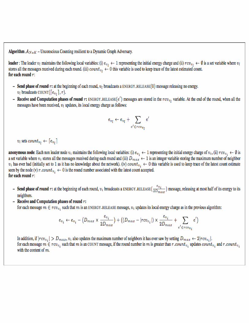
3.1 The No-Knowledge Algorithm ANoK

Frist, I induced a No-Knowledge Algorithm called ANoK, which works in the following

way:

At beginning, at round r0 each non-leader node v has energy quantity ev = 1, then it will

transfer half of its current energy to its the neighbors. But the problem is that the non-leader

nodes v does not have any prior knowledge of the network, before it received the message,

except it can make a guess of the number of neighbors, it cannot get the exact number in r.

Therefore, the non-leader nodes v has to make an assumption that they have d neighbors, and the

broadcast a ½ d energy quantity. After that, v begins to collect messages was sent from its

neighbors at the beginning of the round, then store this message into a local variable Ssmg.

Finally, at the end of the round, non-leader nodes v can update its energy quantity, now the ev

should be ½ + ( d - | Smsg | ) * ½ d + ∑ ∀ m S∈ msg * m to maintain the quantity energy will change

over all the network.

Pay attention to that, when the real number of neighbors is less than what we estimated,

represent as | Nv (r) ≤ d |, then the global energy conserved among all the processes is still

constant, since the non-leader nodes v did the behavior of compensation at the end of the round

according to the effective number of received message. However, when the real number of

neighbors is more than what we estimated, represented as | Nv (r) > d |, then an operation of

releasing of a local surplus of energy will be done. For example, supposed that v has quantity

energy ev, estimated number of neighbors is d = 2, and the real neighbor is Nv(r) = 8. Now, if v

sends ¼ ev to every neighbors, then the energy stored in v will be half of the total amount of

energy transferred, since the transferred energy is 8 * ¼ ev = 2 ev while node v had only ev energy

left. In fact, because node v regulates its local residual energy according to the number of

message received, eventually its residual energy will be negative, but the globally energy is still

conserved.

In the leader, the local surplus of energy (positive/ negative) that the adversary could

create a temporary energy value e, e > | V | or negative. In addition, at each round, the adversary

could change the degree of node such that the convergence of the leader can be avoided. To deal

with these issues, each process need to store the highest number of neighbors that it has ever seen

in the local, so that it can use this number as its estimated degree d. We can see from that the

adversary can create surplus of local energy (positive/negative) is upper bounded by a function f(

| V | ): because the energy’s conservation has to be maintained, and the local surplus is not

infinity it is finite, the worst case adversary cannot infinitely create surplus of local energy, each

node just can increase d at most | V | - 1 times. Hence, it is easy to prove that eventually the

leader need to converge to the value | V |, there were only a finite number of times this

convergence could be delay. Intuitively, the adversary cannot delay too much moves, since when

the energy stored in V \ { vl } is less than a certain value, even in the worst case, then the local

surplus of energy it could create, it is not enough to change the leader count. Therefore, if the

leader counts [ evl ], at each round r , it can be proved that there exists a round r*, after that the

leader will always compute the correct value despite the move of the adversary [2].

However, choosing several consecutive rounds, we can see the leader outputs are always

same count. This is not enough to define a terminating condition as such number can always

influenced by the adversary. Thus, the convergence cannot be detected by the leader. Now, I

assumed that when at round r, the increment of energy is below a threshold t, and then the leader

stops. We can always get a network that has the t+1 size, each node has t residual energy.

Therefore, each increment on the leader energy is below the termination threshold and residual

energy is greater than 1, so when the leader terminates it will miss one node.

Proofs. In the next part, I will show the proof of the algorithm ANoK converges to the exact

count in a finite of number rounds. First of all, I will prove that the dynamic adversary created

the quantities of negative energy is constrained by a function of the network size | V |. After that,

I will prove the leader can get the correct count in a finite number of rounds but such number is

unknown, hence I will use the convergence property to prove it.

Lemma 1. We have a dynamic anonymous graph G(r) = (V, E(r)). In the ANoK algorithm, the

amount of energy that can be created is finite. And, a single node vi V has energy ∈ can

generat at most negative energy, for any round r.

Proof. Now, we consider that a generic node vi V can create negative energy during the ∈

execution period of algorithm. En : { r(i,1), r(i,2), ….., r(i,t)}be the set of rounds in which vi

generates negative energy. Then, our aim is to show the number t is finite. For the generic round

r(i.j) En we should have that | rcv∈ vi | > 2Dmax, with ½ e + (| rcvvi | - Dmax)* ½ e < 0. This express

means that there is | rcvvi | > 2Dmax, and number Dmax will become twice at the end of r(i,j) round.

Because, we have the | rcvvi | ≤ | V | and Dmax ≥ 1, and the condition | rcvvi | > 2Dmax could appear

at most log(| V |) times. Therefore, t ≤ O(log (| V |)). Also, the node vi generated negative energy

e is at most (| rcvvi | - 2Dmax)* e at a single round, and it is maximized when | rcvvi | = | V | and

Dmax = 1.

Lemma 2. We have the dynamic anonymous graph G(r) = (V, E(r)). At any execution period of

ANoK, For any ε R∈ + , there is a round r|V, ε |, then the amount of negative energy could be

transferred to the leader is less than ε in the following rounds.

Proof. Each node can generate the negative energy is based on the energy that the nodes

already possess, because of the invariant on energy. Moreover, the leader received the

monotonically increasing energy, then the absolute value of energy in V \ { v l} is a

monotonically decreasing function of r, if there is no negative energy is generated. The

maximum amount of negative energy that can be created is bounded starting from round r, and

from the previous consideration it is a monotonic function f of . We

know that because f is monotonic exists ε1 such that f (ε1) ≤ ε, therefore, we get that

Lemma 3. We have the dynamic anonymous graph G(r) = (V, E(r)) at an execution period of

ANoK. Then, we have that . Therefore, the algorithm

ANoK is a counting algorithm that respects the convergence property.

Proof. Lemma 2 indicates that there is a round r|V,ε| such that the maximum amount of negative

energy can be created is constrained by a quantity ε that could be made subjectively small in the

network. According to the energy conservation Lemma, the total amount of positive and negative

energy in V \ { vl } is bounded by a monotonically decreasing function of the number of round

at each round. Therefore, we get , which represent that

there exist a round r make with . Then, the variable countvl

will be equal to . This is what I said the algorithm ANoK respects the

convergence property.

In fact, the previous Lemma implicates that there is a round r makes holds

. But, there does not exist any node that has the ability to detect this

condition. Therefore, the algorithm ANoK respects convergence property. In the practical context,

we can use unconscious algorithms, and the application’s safety does not depend on a correct

count and the liveness and fairness need just eventually correct count.

Energy vs Mass Conservation. In the work of Kempe et al. [37], they used a global

invariant – conservation of mass is similar to the idea of energy transfer and the concept of

energy conservation, and a push-only mechanism implement a gossip-based protocol to do the

aggregation. Forget the similarities between those two concepts, the basic graph is based on a

simple function, but the model I used here is controlled by the worst case antagonist. In addition,

in their model the node knows the number of neighbors for the message-exchange in advance,

but in this paper we do not know it. Therefore, they have probabilistic bounds on the

convergence time and each node of the system converges to the average of input value, but I

used the algorithm the leader always absorbs energy converging to the correct count and the

other nodes converge to zero.

3.2 The No-Knowledge Algorithm with Termination Heuristic A*NoK

At here, I will show how to add heuristic to the basic ANoK , then it can create a new

algorithm A*NoK used in the anonymous network that is No prior Knowledge and does have a

termination condition. In this heuristic, the idea is that using the leader to decide when is the time

to make the current count become the final one. This heuristic is according to the assumption that

the graph’s dynamicity I controlled by a random process, which means that a graph where links

change based on a uniform probability distribution, it supposes that the leader has the ability to

observe the notion of flow.

The leader vl will receive some energy from its neighbors at each round r, now we can

write that at each round r the flow of energy to the leader as:

In here, ev(r) represent the energy of node v, at round r, and dmax v (r) represent the maximum

number of neighbors that v has so far. After a certain number of rounds, the leader observed flow

is:

At here, the expression represents nodes, at round r, has seen the average of the

maximum degrees in G, and the ev(r) represents that at round r the average of the energy kept by

all non-leader node.

Notice that, when the leader is lack, in the network the energy will be always balanced

among nodes, and do not forget that the leader is the only node can absorb energy. Thus, the

neighbors of the leader nodes will have less energy than others, since they transferred some their

energy to the leader node without receiving anything from it. Because of the probabilistic nature

of the edges creation process we have and functioning of ANoK, all the non-leader nodes will tend

to have a similar quantity of energy as they will balance the energy surplus. Therefore, we will

have the estimation by the leader as:

Because of the probabilistic nature of the edges creation process, the leader node will see

the same maximum number of neighbors as the other nodes. Hence, we have:

and, substituting we have:

Based on this we get:

At here, represents at round r the estimation of the number of processes done by the

leader in the network and the p(r) is:

.

We have the number count done by the leader at round r, and the

difference Δ(r) is the difference between the energy currently stored in the leader and the

network size estimated with the energy flow, which is computed from

.

Eventually, We can obtain a termination condition as follows: as long as

maintains constant, over the last k rounds, the leader computes the average

and if after k consecutive rounds both the quantity and

is equal to k, then the counting procedure terminates and the leader outputs

k.

3.3 The Local Counting Oracle-based Algorithm ALCO

In order to deal with the problem of the terminating condition, the Lunay et al. [4] stated

the concept of the local counting oracle (LCO) that reports the current number of neighbors at

each round r. Based on such an oracle, there is a counting algorithm called ALCO has been created,

this algorithm has the ability to count the exact number of processes using a finite number of

rounds. In my work, I will introduce a new algorithm, namely A*LCO, this algorithm is created by

a simple modification of ALCO, and then it will work in a practical context. After that I will do a

performance comparison of between the A*LCO and A*NoK,

The ALCO used the main idea is to give every node a color in the graph, then count there

are how many processes have a specific same color. And the computation is done in the

synchronous round. When at the beginning round r0, except the leader will first colors itself with

a color c0, the other node has no color, its color represent by . After that, at each round r, the ⊥

node will have a new color cr, when it satisfied two conditions: with color , and has at least one⊥

neighbor with a not color. Moreover, at any round r, each non leader colored process ⊥

broadcast a unit energy and its color cr , with the current round r and the multi-set containing the

information it has about its neighbors. When the counting algorithm starts at round r0, the leader

knows exactly how many processes has the color c0 as they are its neighbors, the leader colors

them and their number is given by the LCO. At the later round, the leader will initialize a local

variable to collect the energy sending from the colored node as a container. And for transferring

the energy to the leader I used the same mechanism of ANoK, and the access to LCO also make

sure that negative energy cannot be created.

The leader begins to collect energy from the node has color c0, until it makes all of them

has been collected. And after the leader has collected all the energy from the node has color c0, it

can compute a bound B1 on the set of nodes colored with c1, using the node colored by c0

gathered the multi sets of local view. This bound is obtained by multiplied the number of for ⊥

the multiplicity of the multi-set, and the multiplicity obtained using the energy. Thus, the leader

can use this bound B1 to decide when it already collects enough energy to get the correct count

C1 of process with color c1.

At round 2, each node has the color c1 will create a unitary quantity of energy, the

transfer it to the leader, this energy is marked with the local view lw(1), with the color c1 and

round 1.

The leader can compute the multiplicity of neighbors that has id 0 by collecting this

energy, for each node w. Based on this information, when the nodes that has a color c1 collected

the energy is equal to the adjusted bound B1, it can lower the bound B1 till it gets the correct

count C1 of the nodes has the id 1. Using the sum equation C≤1 = C1 + C0, the leader can

compute the multi sets of neighbors of nodes with ids { 0, 1 }. Finally, when this multi-set is

empty, then the leader terminates, if not it uses the same procedure to count nodes that has color

c2 and so on.

3.4 The Local Counting Oracle-based Algorithm with Symmetry Breaking

A*LCO

The Lunay et al. [4] stated that ALCO has the ability to compute an exact count in a finite

time. But, it needs a lot of time to do so. The reason is that before the leader collected more than

one unit of energy, the leader cannot count two nodes have the same color. For example, suppose

that we have y nodes at round r, and they have the same color and same multi-set lv of neighbors.

The leader needs to collect at least y – 1 + ε energy to count the correct multiciplity y of lv, to do

this process need lots of time. But in practice this two nodes may be same if we consider the

history of their local views, which means that the union of all the multi-sets they saw from round

r0 until the current round.

According to the information, and breaking some symmetry in ALCO, I introduced a new

algorithm, called A*LCO. Symmetry breaking is obtained by using an additional parameter,

thinking about all the local views history and it is used to break the symmetry and to

disambiguate processes having the same color. Basically, each non leader process with color ci

≠ computes a round id ⊥ , at each round r.

Therefore, two nodes u, v that have a different multi set of neighbors at round r’ will have a

different ridr for each round r > r’. This ridr will be added together with the other information to

the energy created at round r.

In this modified algorithm, when the symmetry has not been broken by the dynamic

topology in other words, two nodes that at each rounds have the same neighborhood, it is uses

the concept of energy to count. However, if the symmetry has been broken it can count fast.

Assuming that at round r all nodes with cid ≠ have a different rid⊥ r, the leader could collect

information from all necessary nodes in at most V rounds. We can see from the example

presented that if ½ y nodes have different ridr, then the leader need to wait until it collects

of energy, this is faster.

4 Performance Evaluation

Tool. To do this experiment, I used a JAVA simulator – the Jung library [36] to build

the graph data structure. In the graph each node represents a process v, and it shows an interface

consist of two methods:

1) allowing to send a message for round r.

2) allowing t deliver message for round r

In addition, each node also has a queen qv to store the received message. This simulation have a

set of thread, in which one thread Tj takes one to be examined node from a list that contained all

of the nodes, represent as lm, in this round, then remove it from this list and execute the send

message method. And the thread Tj also takes v produced message to adds it to the queues of

Nv( r ). However, if the lm is empty, then there will be a different set of thread to be activated to

deliver message. The thread Tj takes a node v from list ld and regulate the delivery of all the

message that v received and stored in qv during the current round. After all the messages are

delivered to all the processes in qv, then the round terminates and based on the dynamicity model

the topology can be changed. Finally, a new round can start.

Metrics and parameters. There are three key performance metrics we considered:

i) Convergence Time Distribution: at the first round, the algorithm will output the

correct value and defined the convergence time. In the next section, I work on the

probability distribution of the convergence time in order to explain the average

latency before obtained the correct count in this algorithm.

ii) Flow Based Gain Δ: this is the difference between the leader measured that the

size estimated through the flow and the size estimated through the stored energy

in the leader, expressed as .

iii) Error frequency ρ: this represent the incorrect termination

probability that got from the heuristics-based termination condition

present in the previous section.

The below parameters is what I used to evaluate those above metrics:

i) Dynamicity model: there are different types of dynamic graphs to be used to

evaluate the factor influence each metrics.

ii) Edges creation probability p: based on the certain model, this probability

controls the dynamicity of the graph.

I did used different metrics in the networks to evaluate the performance of the algorithm

includes {10, 100, 1000} nodes. In the following section, most of the test results are

come from 1000 independent runs.

4.1 Evaluation of ANoK

Focused on the algorithm ANoK, I did the evaluation on the G(n , p), edge- Markovian

and Duty-cycle-based graphs. First of all, let us focus on the G(n, p) graphs, in which the

connectivity threshold t is obtained bases on the amount of node in the graph, is

. I did the evaluation of this algorithm for several probability p. In

some cases, the probability greater than 2t, then just connected graph instances to be

considered. Otherwise, if the probability smaller than 2t the disconnected graph instances

to be allowed.

Below the figure 1 present the convergence time distribution of the ANoK algorithm

using by G(n, p) graph. We can see from that as we consider disconnected instances the

convergence time becomes worse and worse. Now, notice that although the disconnected

instances exist, the algorithm still can converge to the correct count. And, the increasing

of convergence time is inversely proportional to p. Moreover, because of the existing of

the disconnected instances, there is an increment of the distribution variance.

Figure. 1: ANoK Convergence time distribution on G(n;p) graphs

Next, for the edge-Markovian graph, let the probability of creating an edge same

as the G(n, p) graphs, and modified the probability of deleting an edge to 0.25, pd = 0.25,

pb = f( t ).

The ANoK convergence time distribution displayed in the figure 2, intuitively, we

can compare it with what I show previously with the G(n, p) graph. Moreover, the low

values of edge creation probability is mitigated by the persistence of edges across rounds.

Eventually, the convergence time is less than the G (n, p).

Figure. 2: ANoK Convergence time distribution on edge-Markovian graph

4.2 Evaluation of A*NoK

At here, I do the evaluation of the A*NoK algorithm on te G(n ,p) graphs and Edge-

Markovian graphs. I present several measures related to the heuristic correctness in the figure 3.

Moreover, except the error frequency ρ, I also measured maximum error and the average error, it

is the number of nodes missed compare to the real number of nodes in this graph. Notice that, I

omit some probabilities because they terminate correctly, which is p ≥ ½ p in the graph G(n, p)

and pb ≥ ¼ t in the graph Edge-Markovian. For the disconnected topologies p ≤ ¼ t in the graph

G(n, p) or pb ≤1/8 t in the graph Edge-Markovian, the number of terminated correctly counting

instance is less that 100% and it becomes proportionally worse with the decrease of p. In

addition, there will be a bimodal behavior of the heuristic occurred when ti fails:

i) In the first counting process, the heuristic forces to terminate. Then the leader output

a count, but it was much smaller than the real number of processes.

ii) If the leader accumulated energy is close to the current network size, then the

heuristic fails.

In my work, there was no the heuristic forces to terminate that occurred in a different way

from this two. Also, the table Convergence Detection Time shows that the number of rounds

after the first convergence that the heuristics employs to correctly terminate the count. Now,

we can see that most of time, the heuristic converges is equal to the size of the network as if

on disconnected instances.

Model G(n, p) Edge-Markovain pd=0.25P t/4 t/8 t/16 t/32 t/8 t/16 t/32| V | 10 100 1000 100 100 100 100 100 100

ᵨ 22% 3% 2% 19% 25% 84% 30% 68% 76%

Average Error 2,02 8,96 1 9 44,5 41,4

1 3,12 11,9

Max Error in Nodes 8 96 1 99 99 99 1 99 99σ of Error 2,1166 27,4 0 27,4 48,3 48,

81 14,23 29,73

Convergence Detection Time Average

10,2 100 1000 100 100 100 100 100 100

Convergence Detection Time Max

40 100 1000 100 100 100 100 100 100

Convergence Detection Time Min

10 100 1000 100 100 100 100 100 100

Figure 3. Evaluation of the Termination Correctness. The results are the

outcome of 500 experiments.

4.3 Comparison between ANoK and A*NoK

We know that we can use the flow to estimate the size of | V | to get a faster count. In the

following figure display that the evolution of Δ, I defined before the Δ is the leader measured the

difference between the size estimated through the flow and the size estimated through the stored

energy in the leader, in a temporal perspective 4(a) and an energy perspective 4(b).

Figure 4: Difference between the size estimated with the flow (A*NoK) and the size estimated by looking

to the energy stored at the leader (ANoK) in a G(n, p) network of |V |=100.

When the energy is about half of size of the network at the leader, Δ get the maximum

value. Thus, when p ≥ t the network is connected, the leader can predict the presence of at least

others 17 nodes based on heuristic. Therefore, this approach could answer faster to predicates

likes | V | ≥ t, on connected instance. In fact, the flow-based estimation also can do well on the

disconnected instances only until a specific threshold, after that the gain obtained with the flow

drops to one or two nodes more than the energy estimated the ones.

In addition, the figures tell us that the reason of the termination heuristics work badly on

instances with p ≤ ¼ p. The value falls behind the threshold of 1, if in the leader the energy is

low, or if in the leader the energy is close to the value | V |, then there are two possible

misbehavior will occurred. One is terminated after several rounds from start. One is when Δ falls

behind 1 again, it could terminate near |V |.

In the figure 4(a), it indicates the behavior of Δ along time.

i) p ≥ t, the network is connected, the leader done the counting fast approaches half

of the size of the network, which is the maximum value for Δ. However, the

energy-based count will approach the real size using an exponential time. We can

see it from the exponential decay of Δ. And this behavior is also correct with p < t,

even there is a slower decay of Δ that clear indicates a slower approach to the real

size.

ii) The curves present a high variance for the value of p ≤ t, since the existing of

disconnected topologies give a variance in the convergence time, and the

magnitude is proportional to the inverse of p. Moreover, during the execution the

high variance of the flow that the leader will see will bring the high variance in

convergence.

We can see the same behavior in Edge-Markovian graph in the figure 5. Because of the

less prone to the value p, then the existing of more edges in the edge-markovian graph has a

positive effect on the Δ. Now, we can find a slightly low maximum value for the edge-markovian

process, 17 against 17.3 of the G(n, p) graph.

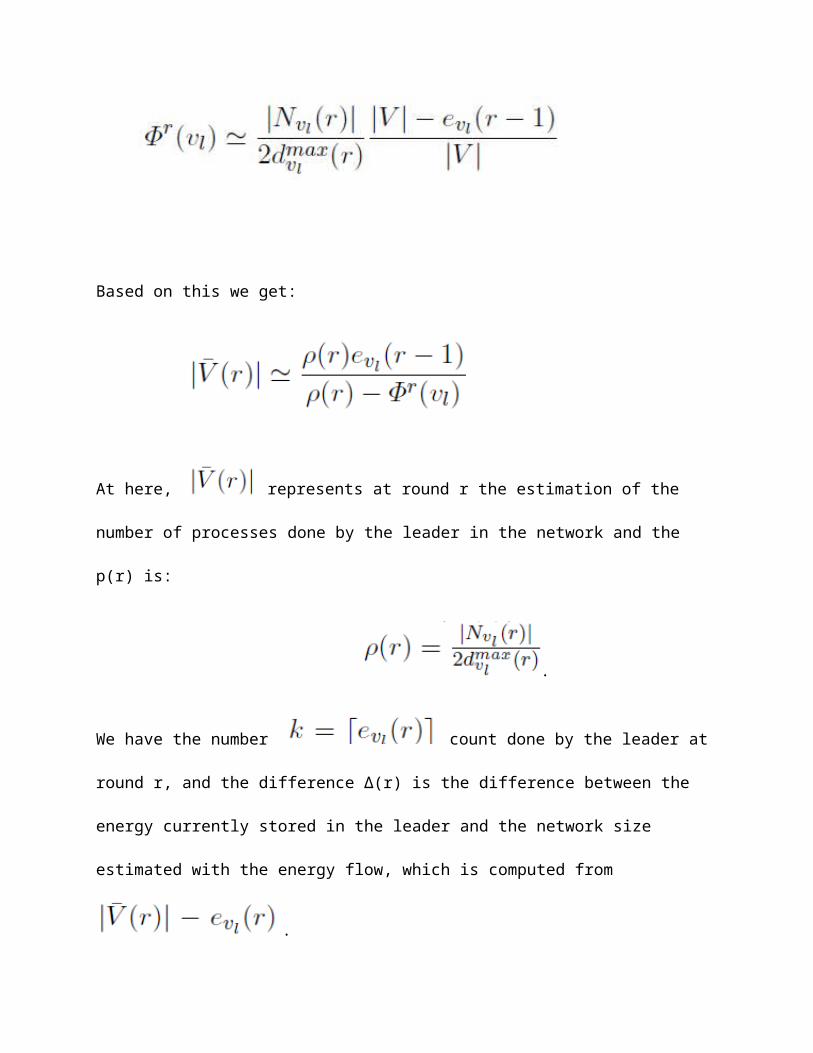
Figure 5: Difference between the size estimated with the flow (A*NoK) and the size estimated by looking to

the energy stored at the leader (ANoK) for Edge- Markovian network with pd = 0:25 of | V |=100.

Notice that, run the test with larger graphs | V | = 100, the curves show the same behavior

like figure 4 and figure 5, and in this case the maximum Δ is about 170 nodes.

4.4 Duty Cycle

Running the algorithm A*NoK on regular topologies to test the adaptiveness of our

heuristic: chains and rings. I use a duty-cycle of eighty percent, over those topologies. Each node

sleeps 20% of the time independently, at this period the links of sleeping nodes will be deleted.

Now, the topology of ring has | V | =100, and the average convergence time is about 26986

rounds over 100 experiments, however, the topology of chain has a convergence time on average

70000 round. Moreover, I have the test of the random G(n, p) topologies with p =2t, it has a

convergence time on average 1059 round for 200 experiments. At this time, we see that the duty-

cycle perform badly both the size estimation and the termination heuristic on graph. For the

chain and ring, the termination heuristic always fails, but on the random graph fail about the 23%

of the instances.

Figure. 6: Difference between the size estimated with the flow (A*NoK) and the size estimated by looking to the

energy stored at the leader (ANoK) of 200 runs for duty cycle and random graph with |V |=100.

4.5 Evaluation of A*LCO

For the each G(n, p), edge-markovian and Random Connected graph, I evaluate the

termination time of the algorithm A*LOC. We know that A*LOC only work on instances are 1-

internval connected. Also, I have the original algorithm ALCO uses15 round with | V | = 10, 393

round with | V | = 100, and 7753 round with | V | = 1000, on average. The figure 7 display that

the performance for the symmetry breaking version. We can easily find that the symmetry

breaking extension allows the algorithm to terminate faster, and the time of termination is

approach to the size of the network. In addition, this indicates that the LCO offered the additional

knowledge allows the counting algorithm to do faster.

Model G(n,p)p = 2t Edge-Markovian Pb =2t Random Connected Graph

|V| 10 100 1000 10 100 1000 10 100 1000

Average Termination 7,6 107,6 1690,6 9,9 113,4 15543,2 10,14 113,8 1559

Max Termination 17 187 2117 19 222 2684 23 220 1899

Min Termination 5 96 1175 5 99 807 6 13 1263

Fig. 7: Termination performance of A*LCO on 1-interval connected instances.

5 Conclusion and Future Works

In this paper, I introduced two new practical algorithms, called A*NoK and A*LCO, which

is modified according to algorithms using the notion of energy transfer, ANoK, ALCO stated in [4].

With those algorithms, I did implement, test and compare among them. From those experiments,

we can see that the algorithm A*NoK not only can terminate correctly on dense graphs, but also it

has a good performances on disconnected instances. Unfortunately, if we use the sparse and

extremely disconnected instances or regular ones where the dynamicity is due to duty-cycling,

then its error rate became high. Moreover, when the heuristic fails, it will have a bimodal

behavior. This problem still need to be studied in the future, I need to figure out how it is

possible to design better heuristics. Because of the concept of energy-flow, the algorithm A*NoK

could answer faster to predicates like | V | ≥ T, becoming a practical use of energy-transfer based

algorithms. In addition, this slow convergence of algorithm ANok on sparse and disconnected

instances could be studied to design algorithms that want to estimate, in a distributed-way, the

edge-density and the connectivity of dynamic anonymous graph with size knowledge. We can

see that from previous work the convergence time seems to strictly depend on the probability

threshold of edge creation p. The algorithm A*LCO does terminate fast on dynamic graphs, and the

dynamicity model of the dynamic graphs is a random adversary, this has a trade-off phoneme

between the knowledge of the network and the counting time.

Reference

1. G. A. DI LUNAy, S. BONOMIy, I. CHATZIGIANNAKISz, R. BALDONIy. Counting in Anonymous Dynamic Networks: An Experimental Perspective

2. G. Di Luna, R. Baldoni, S. Bonomi, and I. Chatzigiannakis. Counting on Anonymous Dynamic Networks through Energy Transfer. Technical Report 1, 2013.

3. Othon Michail, Ioannis Chatzigiannakis, Paul G. Spirakis. Naming and Counting in Anonymous Unknown Dynamic Networks

4. G. A. DI LUNAy, S. BONOMIy, I. CHATZIGIANNAKISz, R. BALDONIy. Counting on Anonymous Dynamic Networks through EnergyTransfer

5. Dana Angluin. Local and global properties in networks of processors (extended abstract). In Proceedings of the twelfth annual

6. ACM symposium on Theory of computing, STOC ’80, pages 82–93. ACM, 1980.7. F Kuhn, N Lynch, R Oshman. Distributed computation in dynamic networks8. H. Terelius; D. Varagnolo; K. H. Johansson. Distributed size estimation of dynamic

anonymous networks9. A. Boukerche; K. El-Khatib; L. Xu; L. Korba. An efficient secure distributed anonymous

routing protocol for mobile and wireless ad hoc networks10. R. Niu; P.K. Varshney. Performance Analysis of Distributed Detection in a Random

Sensor Field11. A. Kimura; E. Kohno; Y. Kakuda. Security and Dependability Enhancement of Wireless

Sensor Networks with Multipath Routing Utilizing the Connectedness of Joint Nodes12. K. Zhao. Dynamic anonymous routing protocol of the Mobile network 13. Perkins, C.; Royer, E. (1999), "Ad hoc on-demand distance vector routing", The Second

IEEE Workshop on Mobile Computing Systems and Applications 14. A Delay-Tolerant Network Architecture for Challenged Internets, K. Fall, SIGCOMM,

August 2003.15. Correctness of a Gossip-based Membership Protocol. André Allavena, Alan Demers and

John Hopcroft. Proc. 24th ACM Symposium on Principles of Distributed Computing (PODC 2005).

16. Rajmohan Rajaraman, Northeastern U.www.ccs.neu.edu/home/rraj/Talks/DynamicNetworks/DYNAMO/June 2006

17. Y. Afek, B. Awerbuch, and E. Gafni. Applying static network protocols to dynamic networks. In Proc. of 28th Symp. On Foundations of Computer Science (FOCS), pages 358–370, 1987.

18. Y. Afek and D. Hendler. On the complexity of gloabl computation in the presence of link failures: The general case. Distributed Computing, 8(3):115–120, 1995.

19. Roger Dingledine, Nick Mathewson, Paul Syverson. Tor: The Second-Generation Onion Router. Usenix Security 2004, August 2004.

20. V. Kostakos. Temporal graphs. Physica A: Statistical Mechanics and its Applications, 388[6]:1007{1023, 2009.

21. J´er´emie Chalopin, Yves M´etivier, and Thomas Morsellino. On snapshots and stable properties detection in anonymous fully distributed systems (extended abstract). In Guy Even and Magn´us Halld´orsson, editors, Structural Information and Communication Complexity, volume 7355 of Lecture Notes in Computer Science, pages 207–218. Springer Berlin / Heidelberg, 2012. 10.1007/978-3-642-31104-8 18.

22. Yun Zhou, Yuguang Fang, and Yanchao Zhang. Securing wireless sensor networks: a survey. Communications Surveys Tutorials, IEEE, 10(3):6 –28, 2008.

23. Masafumi Yamashita and Tiko Kameda. Computing on an anonymous network. In Proceedings of the seventh annual ACM Symposium on Principles of distributed computing, PODC ’88, pages 117–130, New York, NY, USA, 1988. ACM.

24. Christian Scheideler. Models and techniques for communication in dynamic networks. In Proceedings of the 19th Annual Symposium on Theoretical Aspects of Computer Science, STACS ’02, pages 27–49, London, UK, UK, 2002. Springer-Verlag.

25. Naoshi Sakamoto. Comparison of initial conditions for distributed algorithms on anonymous networks. In Proceedings of the eighteenth annual ACM symposium on Principles of distributed computing, PODC ’99, pages 173–179. ACM, 1999.

26. Masafumi Yamashita and Tiko Kameda. Computing on an anonymous network. In Proceedings of the seventh annual ACM Symposium on Principles of distributed computing, PODC ’88, pages 117–130, New York, NY, USA, 1988. ACM.

27. Naoshi Sakamoto. Comparison of initial conditions for distributed algorithms on anonymous networks. In Proceedings of the eighteenth annual ACM symposium on Principles of distributed computing, PODC ’99, pages 173–179. ACM, 1999.

28. P. Fraigniaud, A. Pelc, D. Peleg, and S. P´erennes. Assigning labels in unknown anonymous networks. In Proceedings of the nineteenth annual ACM symposium on Principles of distributed computing, pages 101–111. ACM, 2000.

29. James Aspnes, Faith Ellen Fich, and Eric Ruppert. Relationships between broadcast and shared memory in reliable anonymous distributed systems. Distributed Computing, 18(3):209–219, February 2006.

30. Regina O’Dell and RogertWattenhofer. Information dissemination in highly dynamic graphs. In Proceedings of the 2005 joint workshop on Foundations of mobile computing, DIALM-POMC ’05, pages 104–110, New York, NY, USA, 2005. ACM.

31. Othon Michail, Ioannis Chatzigiannakis, and Paul G. Spirakis. Brief announcement: Naming and counting in anonymous unknown dynamic networks. In DISC, pages 437–438, 2012.

32. Othon Michail, Ioannis Chatzigiannakis, and Paul G. Spirakis. Causality, influence, and computation in possibly disconnected synchronous dynamic networks.

33. In Roberto Baldoni, Paola Flocchini, and Ravindran Binoy, editors, OPODIS, volume 7702 of Lecture Notes in Computer Science, pages 269–283. Springer, 2012. P. Boldi and S. Vigna. Computing anonymously with arbitrary knowledge. In PODC, pages 181–188. ACM, 1999.

34. M. Jelasity, A. Montresor, and O¨ . Babaoglu. Gossip-based aggregation in large dynamic networks. ACM Trans. Comput. Syst.,23(3):219–252, 2005.

35. D. Kempe, A. Dobra, and J. Gehrke. Gossip-based computation of aggregate information. In FOCS, pages 482–491, 2003.

36. Jung. http://jung.sourceforge.net/, 2013.37. D. Kempe, A. Dobra, and J. Gehrke. Gossip-based computation of aggregate information.

In FOCS, pages 482–491, 2003.