Home Market effect and National Income

Martin Tobal

Abstract

In this article I develop a 2 good-2 country model in general equilibrium where firms with increasing returns to scale make positive profits even though they interact in a classic monopolistic competition environment. This model provides new answers to three important questions: first, what is the relevance of a country’s size on its pattern of trade? Second, what are the welfare consequences of that pattern when there are income sources besides labor earnings? And third, what are the real incentives for a country to increase its tariff on foreign products?. Relative to the new international trade policy theory, my model makes a great contribution: because I break the free entry assumption down, it uncovers the welfare consequences of firm location created by profits and the new resulting taxation motivations. Even more, as free entry is not considered, my model, as opposed to the new international trade policy settings, becomes a tool to study regional antitrust policies. Relative to the standard international trade policy theory, my theory makes two important contributions: it allows for product differentiation in a non-oligopolistic framework and for market interaction.

1. Introduction

“Our obligation is to support and protect Spanish firms”. This statement was made by the Spanish president, Jose Luis Rodriguez Zapatero, in a plenary session of the Spanish senate in November of 2008. The sentence summarized his disagreement with the possibility of a Russian firm’s acquiring the largest Spanish company, Repsol.

The statement is just an example of two apparent major goals in a government’s policy. First, governments, such as Zapatero’s administration, do not want national firms to “change their flags” in favor of other nations. Second, they tend to promote the growth and health of national companies, in particular of those selling national products abroad and “capturing” foreign income. “As many and as profitable national firms as possible” seems to be the principle.

Although usually fudged under other labels, such as that of “strategic sectors”, it is natural to think that one important motivation for this principle is the increase in national income resulting from firms’ making positive profits. A country’s firms having higher profits traduce into a greater national income and then into higher levels of national welfare.

Even if the desire to protect national firm profits and to increase its number seems hard to deny, this motivation is left aside in most of the international trade theory in general equilibrium i1. In particular, this incentive is absent in the Krugman model (1980), which triggered the so called “new trade theory”.

The main reason for this absence is that these models work in a classic monopolistic competition environment, where free entry ensures that the zero profit condition holds. The main implication of this absence is that governments’ incentives in designing their trade policies do not reflect their wish to attract firms to increase national income.

My model recognizes that labor earnings are not the only source of national income. The existence of entry barriers at a regional level prevents firms’ profits from dropping to zero.

The forces lying behind the entry barriers assumption can be found in many of the standard domestic industrial organization arguments when applied to a region instead of to a single country. As it is well known, patents and licenses are examples of these arguments whose use was extended after the strengthening of intellectual property protection that followed the WTO birth.

By breaking the free entry assumption down, this model’s results replicate some features of the observed situations in sectors related to the protection of intellectual property. In particular,

1 Helpman, E., M. J. Melitz, and Y. Rubinstein. ( 2008) considers profits greater than zero but they are forced to introduced firm heterogeneity and uncertainty.

under some parameter restrictions, their equilibria are situations where firms serve both the home and the foreign markets and make positive profits at the same time.

There have been some attempts in the literature to introduce entry barriers and positive profits in a General Equilibrium model. However, to the best of my knowledge, all the efforts have been concentrated in modeling oligopolistic competition together with market interactions. In fact, Neary(2002)2 accomplished the challenge by assuming “continuum quadratic” preferences, which makes firms’ reaction functions tractable.

In Neary’s (2002), entry barriers are introduced in each of the homogenous products composing the continuum of goods. His approach, though, is quite different from mine. He considers firms’ interactions and focuses on the effect of comparative advantage on trade by assuming no trade costs and a Ricardian cost structure. On the other hand, although I do not consider firms’ strategic behavior, I do not depart that much from the standard new trade theory assumptions –IRS, differentiated product and Love for variety- and focuse on the welfare effects of trade barriers and antitrust policies.

There exist three main consequences of recognizing the existence of entry barriers. The first is that the major Krugman model’s result is completely modified. Although in my model, as in Krugman’s, the increase in a country’s share of world labor supply traduces into a greater number of national varieties, the world economy does not expand along with an increase in total varieties .

In other words, when a nation’s labor endowment goes up, in my model national firms’ profits increase too. This increase makes foreign firms change their location but, as opposed to Krugman’s, entry barriers do not allow for the world number of firms to be higher. In this context, the economy expands through the augmentation of each variety’s production–and each firm’s profits- and not through a wider range of varieties.

The second main consequence of entry barriers introduction is that because the number of world variety producers is fixed and exogenous, there is room for antitrust policy. In this sense, the model makes a great contribution: while the standard model does not allow for such investigation, this new setting can be used to study the differential welfare impact of regional antitrust policies such as that of the E.U. As a matter of fact, the comparative statics shows that making markets less concentrated may benefit small countries.

The third main consequence of entry barriers introduction is that a nation’s incentives to increase tariffs -which take the form of Samuelson (1952) ii “Iceberg Costs”- in my model reflect the principle of “as many and as profitable national firms as possible”.

2 “International Trade in General Oligopolistic Competition”, 2002, Unpublished. http://www.economics.ox.ac.uk/Members/peter.neary/neary.htm#unpub

As Ralph Ossa (2008) highlights, in the standard Krugman model governments’ incentives to increase tariffs unilaterally come from the implied rise in the number of national products. In Ossa’s model, that founded the new international trade policy, that rise in the number of national firms just makes smaller the range of varieties over which national consumers pay Iceberg costs. My model, though, also considers the augmentation in national income derived from the tariff increase.

In this sense, my model represents a reconciliation of the new trade theory with the standard international trade policy theory triggered by the publication of the Brander and Spencer ‘s (1984) seminal paperiii.

The emergence of this policy theory in the eighties shows that economists started to recognize that trade policy could be used to artificially create advantages for national firms and increase national income. In this literature, the closer concept to my principle of “as many and as profitable national firms as possible” is called the “Rent Shifting” motivation.

Dixit (1984) ivanalyses the governments’ incentives to determine import tariffs, export subsidies and production subsidies; on his article shifting rent is one of those motivations. In his model, firms run into a Cournot competition into separated markets, the demand curves in the two markets are independent. This does not happen in my model, that departs from a General Equilibrium Krugman environment.

Not just tariffs and subsidies have been subject of study, but many policy instruments have been considered in this literature. Krishna (1983)v, for example, builds a duopoly model where governments are allowed to impose an import quota. Because this quota prevents the Foreign firm to undercut the home’s firm price and sell more, the national company finds it profitable to raise its price. What all articles in this literature have in common is the recognition of the rent shifting motivation and the partial equilibrium scenario.

As explained above, my theory takes the “Rent Shifting” incentive into account also, so, in this sense, it is closely related to the eighties literature. However, the channel through which rent shifts from one country to another in my model differs considerably from the channel described by the standard international trade policy theory.

In my model the number of firms in each country is not taken as given, I let companies choose their location. Not only is this assumption more realistic –in particular from the mid nineties on- but it also has a dramatic implication: a firm’s profits remain the same no matter what the tariffs are. The increase in Iceberg costs only makes some firms shift from country to another, which is to say, the “Rent shifting effect” only occurs through the “Krugman channel”.

A second contribution to the literature triggered by Brander and Spencer is that my model is set in a general equilibrium framework, as opposed to the eighties literature. This has important advantages regarding market interactions and welfare measurement, which can be worked out

straight from a representative consumer’s indirect utility function; I am not forced to restrict myself to national profits.

Finally, as when compared to Neary’s paper, one difference between the eighties literature and this paper is the form of competition; here it is not oligopolistic but monopolistic, which lets me work with a C.E.S. function and consider consumers’ love for variety. As I said, the drawback from this approach is that I lose firm’s strategic interaction.

Next 2 Paragraphs to be written:

I develop my model in the remainder of this paper. In the next section, the basic two-country two-good model is introduced. In this section I also present the first model parameter conditions and give intuition for these restrictions. In Section 2.2. I make the assumption of both countries having the same tariffs, approach the stability problem of the model, find the equilibrium and show the main comparative static results.

In Section 2.3. I break the equal across country tariff assumption and proceed talking about the equilibrium. I focus especially on how changes in the tariffs modify the equilibrium endogenous variables. Finally, in section 3 I draw the main conclusions of the model.

2. Basic Model

2.1. Set up

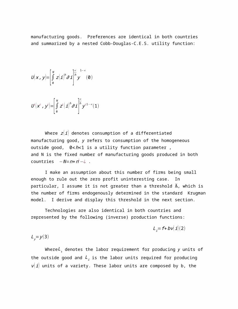
I consider the case of two countries: Home and Foreign. Variables that refer to Foreign are identified by a superscript asterisk (*). Consumers’ utility in both countries depends on a composite good and a single homogeneous “outside good”. The composite product is composed by a continuum of differentiated manufacturing goods. Preferences are identical in both countries and summarized by a nested Cobb-Douglas-C.E.S. utility function:

U ( x , y )=[∫0N

z ( i )h∂i ]∝hy1−∝

(0)

U ¿ ( x¿ , y¿)=[∫0N

z¿ (i )h∂ i ]∝hy¿1−∝(1)

Where z (i ) denotes consumption of a differentiated manufacturing good, y refers to consumption of the homogeneous outside good, 0<h<1 is a utility function parameter , and N is the fixed number of manufacturing goods produced in both countries −N=n+n¿−¿ .

I make an assumption about this number of firms being small enough to rule out the zero profit uninteresting case. In particular, I assume it is not greater than a threshold N , which is the number of firms endogenously determined in the standard Krugman model. I derive and display this threshold in the next section.

Technologies are also identical in both countries and represented by the following (inverse) production functions:

Li=f +bv (i)(2) Ly= y (3)

WhereLy denotes the labor requirement for producing y units of the outside good and Li is the labor units required for producing v ( i ) units of a variety. These labor units are composed by b, the marginal labor requirement, and f, which denotes the fixed labor requirement. Monopolistic competition takes place on the manufacturing goods market and perfect competition on the outside good market.

When a unit of a variety arrives to a country from the other, τunits were delivered by the latter. That is to say, τ−1 units melt away during the trip; trade costs exist only for manufacturing goods and are of the Samuelson iceberg type. These iceberg trade costs can be thought as trade barriers, which can be either identical - section 2.2- or different -section 2.3- across countries, plus trade costs, which are always identical.

When allowing for different trade barriers, they can be interpreted as policy instruments. Then, tariffs, in particular, become a special case of trade barriers in the sense that they impede trade.

Although in this paper sometimes I refer to trade barriers as tariffs, I do not take into account the revenue they generate in order to keep the generality of the model. This, as Ralph Ossa (2008)vi points out, is essential for the model’s tractability and lets us generalize every argument in this paper to the case of any impediment to trade created by a government’s decision. Finally, the range of considered tariffs is determined by the interior solution and the stability conditions displayed in the next sections.

2.2. Equal Trade Costs

A-Basic assumptions

In this sub-section, I derive the demand and supply sides of the model. I use the model demand to get the indirect utility function and both sides to find out the threshold N . From this threshold, I make the parameter assumption that guarantees positive profits in equilibrium . I also derive conditions on the relative labor endowments, which ensures that corner solutions are not equilibria. In the next sub-section, I solve the model and study its equilibrium properties.

To derive the demand and supply model sides, I first choosew=w¿=1 3, where w is the wage rate. Then I get the following definitions for national incomes:

I=L+nπ (4 ) I ¿=L¿+(N−n )π¿ (5 )

Where I refers to national income and π to the profits made by any national firm. Notice that in these income definitions, I am assuming there are not any capital flows between the two countries. Even if strong, this assumption is not crucial: if part of the profits made by foreign firms at home was rebated to their home-nation, the former would still benefit from firm location. Then the new mechanisms discovered in this model would still exist.

Next, I derive the model supply side. For this, I remind that, as shown by Krugman (1985) vii , utility maximization with the preferences displayed in (0) and (1) yields manufacturing good demands

with constant elasticity equal to −θ= −11−h 4. Because this elasticity is constant, by profit

maximization, the mark-up over the marginal cost for variety producers is also constant and equal to:

(θ

θ−1)b=b

h=p(6)

Where θ

θ−1=1

h is the mark-up and p is the price of either a national or a foreign variety.

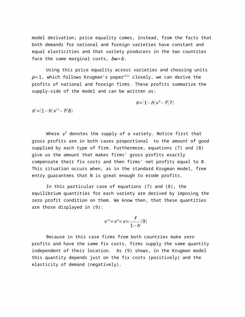
Notice that we are not imposing the price for foreign and national varieties to be equal, which would be the case if we imposed an interior solution at this stage of the model derivation; price equality comes, instead, from the facts that both demands for national and foreign varieties have constant and equal elasticities and that variety producers in the two countries face the same marginal costs, bw=b.

Using this price equality across varieties and choosing units p=1, which follows Krugman’s paperviii closely, we can derive the profits of national and foreign firms. These profits summarize the supply-side of the model and can be written as:

π=(1−h ) vs−f (7) π¿=(1−h ) v¿s−f (8)

3 Actuallyw=w¿=1 , factor price equalization is guaranteed by the conditions imposed to the parameters, under which the two sectors are active in both countries. 4 Since there is no firm heterogeneity, they all make the same profits.

Where vs denotes the supply of a variety. Notice first that gross profits are in both cases proportional to the amount of good supplied by each type of firm. Furthermore, equations (7) and (8) give us the amount that makes firms’ gross profits exactly compensate their fix costs and then firms’ net profits equal to 0. This situation occurs when, as in the standard Krugman model, free entry guarantees that N is great enough to erode profits.

In this particular case of equations (7) and (8), the equilibrium quantities for each variety are derived by imposing the zero profit condition on them. We know then, that these quantities are those displayed in (9):

v¿s=vs=v= f1−h

(9)

Because in this case firms from both countries make zero profits and have the same fix costs, firms supply the same quantity independent of their location. As (9) shows, in the Krugman model this quantity depends just on the fix costs (positively) and the elasticity of demand (negatively).

However, in this paper, because free entry is not assumed, firms’ equilibrium quantities depend also on N, the exogenously determined number of firms. The higher this parameter, the more intense competition is and, therefore, the lower equilibrium quantities are.

From this last statement, we know that if I were to rule out the zero profit case, N should be

low enough in order for each variety equilibrium quantity to be greater than f1−h , the output level

that makes profits equal to zero. In the next paragraphs, I dig into the demand side of the model and leave (11) aside, which I will use it later in the N threshold derivation.

Once that price equality across varieties was established, the units were chosen and the national incomes defined, we are ready to write the demands for foreign and national varieties:

z (i )1 , d+z (i )2 ,d=[ 1g ]αI+ρ[ 1g¿ ]α I ¿(10)

z¿ ( i )1 ,d+z¿ ( i )2 ,d=ρ [ 1g ]αI+[ 1g¿ ]α I¿ (11)

Where z (i ) j ,d denotes country j’s consumers demand for the national variety i,

ρi=τ i1−θ∃(0,1) is a measure of the iceberg trade costs and I and I ¿ follow definitions (7) and (8).

In (10) and (11) the price indices are given by:

P=g11−θ=[n+n¿ ρ ]

11−θ (12)

P¿=g¿ 11−θ=[nρ+n¿ ]

11−θ (13)

Finally, to fully display the model demand side, I show the demand for the homogenous good:

yd=(1−∝ ) I (14 ) y¿d=(1−∝ ) I ¿(15)

Equations (10) - (15) summarize the demand-side of the model. I next use this information to derive first the indirect utility and the threshold N . Plugging the demand functions on (0) and (1) yields the following indirect utility functions:

V=∝∝(1−∝)∝g(1−h)∝

h I (16)

V ¿=∝∝ (1−∝ )∝ g¿( 1−h)∝

h I¿ (17)

To get N threshold, I use equations (10) - (13). Notice on these equations that both the total demand for a national variety (10) and that for a foreign manufacturing good (11) depend on n through the income and the price index definitions. By imposing market clearing conditions, this dependence, together with (9), which shows each variety’s equilibrium supply under the free entry assumption, can be used to work N out.

In fact, N is just the n value that clears the national and foreign variety markets. This way, in the standard model N (n+n¿¿ is determined by the cost and demand parameters. In the next paragraphs, I derive N as if it were endogenously determined and impose N<N . In the next subsection, I exogenously fix N by using this condition and solve the model.

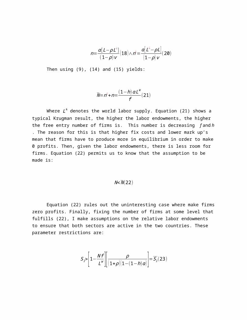
Under the zero profit conditions -and then (9)-, definitions (4) and (5) become I=L and I ¿=L¿. Plugging these two national income definitions and (12) and (13) in (10) and (11) gives us two new equations we can use to solve for our two unknowns: n∧n¿. Solving this system yields:

n=α [L−ρ L¿](1−ρ)v

(18 )∧n¿=α [L¿−ρL ]

(1−ρ ) v(20)

Then using (9), (14) and (15) yields:

N=n¿+n=(1−h)α LW

f(21)

Where LW denotes the world labor supply. Equation (21) shows a typical Krugman result, the higher the labor endowments, the higher the free entry number of firms is. This number is decreasing f and h . The reason for this is that higher fix costs and lower mark up’s mean that firms have to produce more in equilibrium in order to make 0 profits. Then, given the labor endowments, there is less room for firms. Equation (22) permits us to know that the assumption to be made is:

N<N (22)

Equation (22) rules out the uninteresting case where make firms zero profits. Finally, fixing the number of firms at some level that fulfills (22), I make assumptions on the relative labor endowments to ensure that both sectors are active in the two countries. These parameter restrictions are:

Sl>[1−N fLW ] [ ρ

(1+ρ ) (1−(1−h)α ) ]=S l(23)

Sl<1−[1− N fLW ][ ρ

(1+ρ ) (1−(1−h)α ) ]=Sl(24 )

Equation (23) ensures that not all firms want to locate at the foreign country. Notice that the first factor on the right side is positive whenever (24) holds and the second factor is always positive because 1>(1−h )α. From (23) and (24), it can also be seen that the labor endowment restrictions here are generalizations of those of the standard model. For this, just plug

N=(1−h)α LW

f=N in (18) and (19) and get:

ρ1+ ρ

<sl< 11+ ρ

(25)

Equations (23) and (24) collapse to the standard model parameter restrictions when N=N as shown in equation (25). Both sets of conditions reflect that the national relative market size –given bysl - matters for firms when deciding where to locate. Notice, though, that one important difference between the two sets is that while α and h do not show up in (20), they appear in (18) and (19) together with N , which in this model is exogenous.

The last assumption in this section is made on the absolute labor endowment values. When (21) and (22) hold, the homogeneous good sector is active in both countries. The assumptions are:

L>[hα LW+(1−α )N f1−(1−h)α ](26) L¿>[ hα LW+(1−α)N f

1−(1−h)α ](27)

Notice that equations (24) and (26) and (23) and (27) can be jointly satisfied if given the other parameters, α is low enough. In fact this happens if α is given by (28):

α< 11+ ρ

(28)

The intuition for this is similar to that in Ossa’s paper and goes as follows: for both sectors to be active in a country, a sufficient condition is that its labor endowment is high enough to produce all the varieties there and yet some homogeneous good. Since the total production of varieties in equilibrium –and then the required amount of labor- is decreasing in α , a low value makes (26) and (27) less restrictive and (23) and (24) easier to satisfy given the other parameters. Although (28) is enough to make both sectors be active in the two countries, I next make a stronger assumption to simplify the set of restrictions to be imposed. When (28) holds, not only (23) and (27) can be jointly satisfied, but, as a matter of fact, under (22), (23) is implied by (27). Equation (29) is:

α< ρ1+ ρ

(29)

As a reminder, both sectors being active in the two countries guarantees that the national and the foreign wage rates are equal due to the homogeneous good price equalization –derived from no trade costs in the sector- and the CRS specification. This is consistent with the fact that we set both rates to 1 at the beginning of this section.

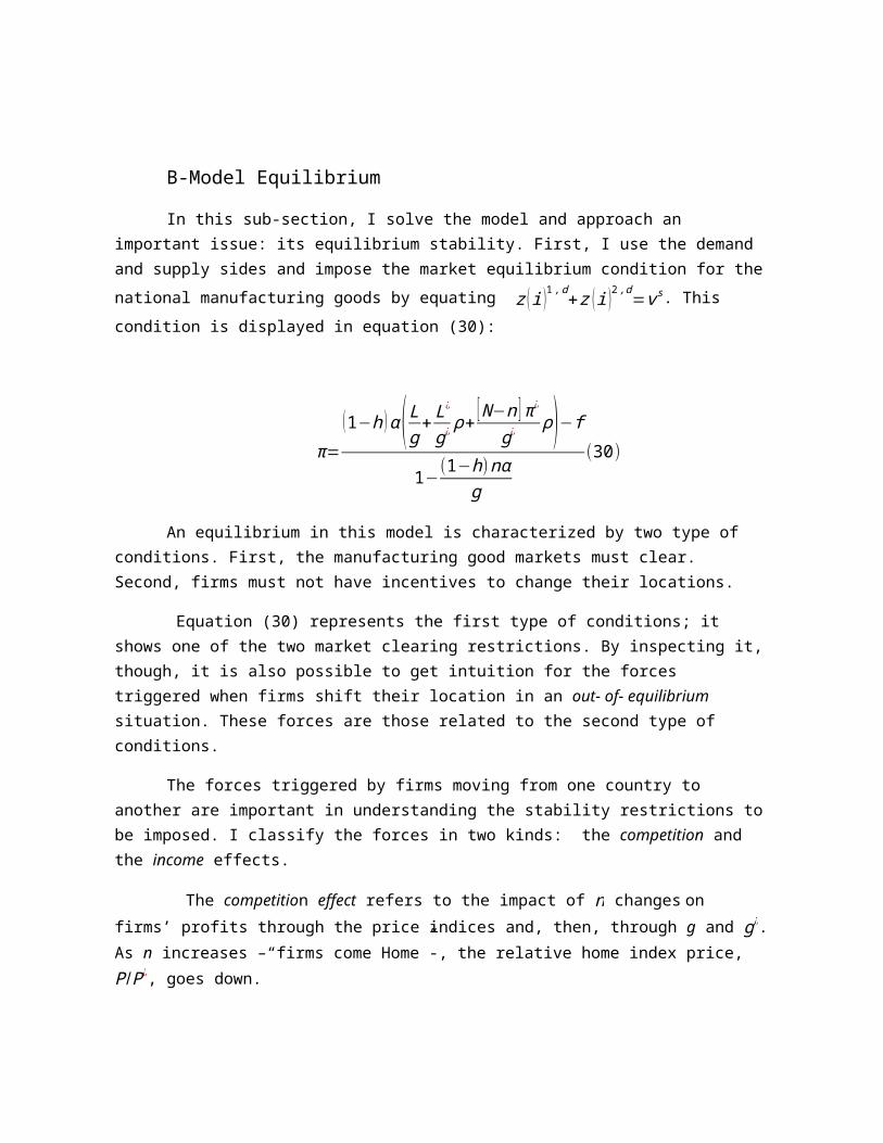
B-Model Equilibrium

In this sub-section, I solve the model and approach an important issue: its equilibrium stability. First, I use the demand and supply sides and impose the market equilibrium condition for the national manufacturing goods by equating z (i )1 , d+z (i )2 ,d=vs. This condition is displayed in equation (30):

π=(1−h )α( Lg + L¿

g¿ ρ+ [ N−n ] π¿

g¿ ρ)−f

1−(1−h)nα

g

(30)

An equilibrium in this model is characterized by two type of conditions. First, the manufacturing good markets must clear. Second, firms must not have incentives to change their locations.

Equation (30) represents the first type of conditions; it shows one of the two market clearing restrictions. By inspecting it, though, it is also possible to get intuition for the forces triggered when firms shift their location in an out- of- equilibrium situation. These forces are those related to the second type of conditions.

The forces triggered by firms moving from one country to another are important in understanding the stability restrictions to be imposed. I classify the forces in two kinds: the competition and the income effects.

The competition effect refers to the impact of n changes on firms’ profits through the price indices and, then, through g and g¿. As n increases –“firms come Home”-, the relative home index price, P/P¿, goes down.

The reason is that since the number of national firms goes up and that of foreign goes down, consumers at home pay trade costs over a smaller range of varieties. The intuition for the impact of this P/P¿ decrease on firms’ profits goes as follows: the “old national firms” share the benefit from

serving the national market without costs with the “new national firms”. Therefore, as n increases, the national manufacturing good market becomes more competitive (and the foreign market less).

In terms of equation (30), this effect is represented by a g increase and a g¿ decrease , which tend to make national firms’ profits smaller.

The Income effect refers to the impact of n changes on firms’ profits through changes in II ¿ .

Ceteris Paribus, as n increases total national profits (nπ ¿ go up, which makes makes II ¿ augment.

Since demands depend on incomes, this augmentation traduces into a higher relative demand for national manufacturing goods.

In terms of equation (30), this effect is represented by a denominator decrease. Notice that this tends to make national firms’ profits greater. Even more, this effect acts in a “multiplier way”: as firms install at Home, they make the relative demand for national manufacturing goods higher, which makes firms move to Home and so on.

The fact the Income effect takes this multiplicative form raises an important issue, the stability of the model, which I address in the next paragraphs. To approach the model stability issue, I consider the three types of possible equilibria: the two corner solutions and the interior equilibria.

In the particular interior solution case, across-country profit equalization is a necessary condition for equilibrium. Firms’ profits must be equal in both countries in order for them not to want to move if varieties are being produced everywhere5. This profit-equalization, though, is not sufficient for stability.

To see what is required for an interior equilibrium ¿) to be stable, define n∃¿) as the “Zone Of Interest”, where n1

¿ is the closest equilibrium to the left (n2¿>n1

¿ ) of n2¿ and n3

¿ is the closest

equilibrium to the right (n2¿<n3

¿ ) of n2¿.

Checking the conditions for an interior equilibrium to be stable requires studying the “Zone Of Interest”. In particular, we need any national firm’s profits to be greater than a foreign firm’s for every n such that n2

¿>n>n1¿ . This guarantees that for every n such that n2

¿>n, firms want to move

home and that n converges to n2¿. Equivalently, we also need firm’s foreign profits to be greater for

every n such that n3¿>n>n2

¿ .

Notice that if there exists just one interior equilibrium, the condition for it being stable is equivalent to that of being the only equilibrium at all. To see this, notice that, in this case because there is just one interior equilibrium: n1

¿=0 and n3¿=N . Then stability of the interior solution

5 These demands are shown in (10) and (11).

requires that at n=0 (n=N ), a home (foreign) firm’s profits are greater than a Foreign (Home) firm’s. But this means that n=0 and n=N are not equilibria because companies can increase their profits by changing their locations when either n=0 or n=N .

From a theoretical point of view there is no guarantee that interior equilibria are always stable. In fact, if the income effect is stronger enough than the competition effect, the model would be unstable because, as firms moved to a country, they would make that nation firms’ profits greater, which would attract even more firms. This means that to get stability, constraining the model parameters to a certain range is required.

However, when there is just one interior equilibrium, the link between its uniqueness and its stability makes it unnecessary to add extra conditions to those already imposed. By means, if there is one and just one interior equilibrium, equations (18) and (19) guarantee non-corner solutions and stability.

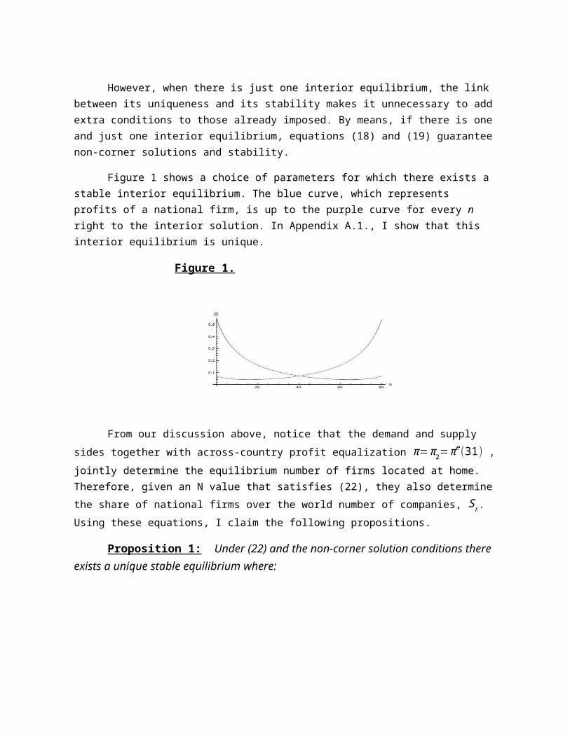
Figure 1 shows a choice of parameters for which there exists a stable interior equilibrium. The blue curve, which represents profits of a national firm, is up to the purple curve for every n right to the interior solution. In Appendix A.1., I show that this interior equilibrium is unique.

Figure 1.

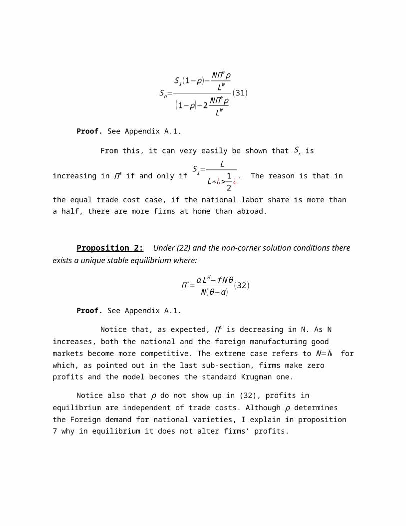
From our discussion above, notice that the demand and supply sides together with across-country profit equalization π=π2=πe (31) , jointly determine the equilibrium number of firms located at home. Therefore, given an N value that satisfies (22), they also determine the share of national firms over the world number of companies, Sn. Using these equations, I claim the following propositions.

Proposition 1: Under (22) and the non-corner solution conditions there exists a unique stable equilibrium where:

Sn=Sl(1−ρ)−N Π e ρ

LW

(1−ρ )−2 N Π e ρLW

(31)

Proof. See Appendix A.1.

From this, it can very easily be shown that Sn is increasing in Π e if and only if

Sl=L

L∗¿>12¿ . The reason is that in the equal trade cost case, if the national labor share is more

than a half, there are more firms at home than abroad.

Proposition 2: Under (22) and the non-corner solution conditions there exists a unique stable equilibrium where:

Π e=α LW−f N θN (θ−α )

(32)

Proof. See Appendix A.1.

Notice that, as expected, Π e is decreasing in N. As N increases, both the national and the foreign manufacturing good markets become more competitive. The extreme case refers to N=N for which, as pointed out in the last sub-section, firms make zero profits and the model becomes the standard Krugman one.

Notice also that ρ do not show up in (32), profits in equilibrium are independent of trade costs. Although ρ determines the Foreign demand for national varieties, I explain in proposition 7 why in equilibrium it does not alter firms’ profits.

Corollary 1: Under (22) and the non-corner solution conditions there exists a unique stable equilibrium where:

Sn=Sl (1+ρ ) (1−(1−h)α )+ ρ(N f

LW −1)

(1+ρ ) (1−(1−h)α )+2ρ (N fLW −1)

(33)

Proof. By propositions 1 and 2.

As expected, the equilibrium Sn is increasing in Sl : as home’s labor endowment increases, variety producers have more incentives to locate there and serve a higher demand without trade costs. This incentive increase traduces into a higher Sn .

In fact, the conditions for ∂Sn

∂S l being greater than 0 are exactly (18) and (19). Therefore,

whenever 0<Sn<1, we have ∂Sn

∂S l>0.

Notice also that Sn depends on firms’ fix costs and their mark-up through equilibrium profits.

Proposition 3: In a stable interior solution equation (22) guarantees that ∂Sn

∂S l is

greater than in the Krugman standard model.

Proof. See Appendix A.3.

Figure 2. depicts the equilibrium Sn as a function of Sl. The blue line refers to the case where N=N , while the purple and the grey show cases where N is smaller (N grey<N purple¿. From inspection, the grey line’s slope is steeper than the purple’s and that than the blue’s.

Following the literature, this result can be interpreted as a “Reinforced Home Market Effect”, by means that an increase in a country’s market size traduces into a higher augmentation of its variety world share: markets’ sizes become more important when there is no free entry.

Notice that equation (22) is the one that ensures the reinforcement of the Home market effect. This equation guarantees that firms are making profits and then that the income effect takes place. This effect is the ultimate reason for the reinforcement.

To see why the reinforcement occurs, first consider the Krugman model case. As Sl goes up

from an initial equilibrium, the standard mechanism acts: because II ¿ increases, firms have

incentives to move home and serve a greater market without costs. This is the end of the process in the standard model.

However, in this new setting because firms make positive profits, the location of new firms

associated to the standard mechanism is another source of II ¿ increase. Therefore, because of the

income effect, in this model a Sl augmentation gives firms more incentives to move.

Figure 2

Proposition 4: In a stable interior solution, ∂Sn

∂ N is negative if sl>

12 .

Proof. See Appendix A.2.

This result can also be seen in Figure 2. Notice that the three lines intersect at sl=12 . This

means that departing from a situation such as that described by the purple line to another described

by the grey, a country’s share would increase if sl>12 : for any sl such thatsl>12 the grey line is up to

the purple.

This result is better understood if the comments on Propositions 1 and 2 are considered. First, I remind that, as pointed out in proposition 2, an N increase makes equilibrium profits (Π e)

lower because both markets become more competitive. I also remind that If Sl>12 (¿

12), there are

more national (foreign) than foreign (national) firms as claimed in Proposition 1: Sn>12 .

When Sn>12 , a profit equilibrium (Π e) reduction implies both

II ¿ and national relative

demand decreases. Since this motivates firms to leave the country, an N increase is associated to a lower (higher) Sn.

When understood as N increases, antitrust regional policies reduce the number of firms in the big country and increase it in the small one.

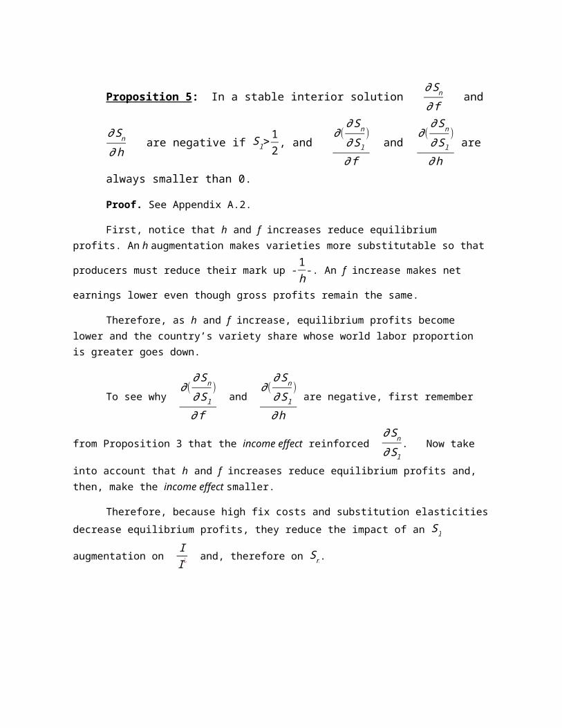
Proposition 5: In a stable interior solution ∂Sn

∂ f and

∂Sn

∂h are negative if Sl>

12 , and

∂(∂Sn

∂S l)

∂ f and

∂(∂Sn

∂S l)

∂h are always smaller than 0.

Proof. See Appendix A.2.

First, notice that h and f increases reduce equilibrium profits. An h augmentation makes

varieties more substitutable so that producers must reduce their mark up -1h -. An f increase makes

net earnings lower even though gross profits remain the same.

Therefore, as h and f increase, equilibrium profits become lower and the country’s variety share whose world labor proportion is greater goes down.

To see why ∂(

∂Sn

∂S l)

∂ f and

∂(∂Sn

∂S l)

∂h are negative, first remember from Proposition 3 that the

income effect reinforced ∂Sn

∂S l. Now take into account that h and f increases reduce equilibrium

profits and, then, make the income effect smaller.

Therefore, because high fix costs and substitution elasticities decrease equilibrium profits,

they reduce the impact of an Sl augmentation on II ¿ and, therefore on Sn.

Proposition 6: In a stable interior solution, ∂Sn

∂ ρ is positive if Sl>

12 , and

∂(∂Sn

∂S l)

∂ ρ

and is always greater than 0.

Proof. See Appendix A.2.

This proposition replicates one the main Krugman’s results: as ρ goes up, trade costs go down6 and the world economy approaches to free trade, which makes Sn more sensitive to the

6 In a corner solution this statement is not true, profit equalization does not need to hold.

relative market size given by Sl. This is because trade costs become less important in determining each market’s attractiveness for firms. Therefore, as ρ goes up the share of the nation whose labor proportion is greater becomes higher.

As pointed out in Proposition 2, thisρ increase does not alter equilibrium profits. Firms’ moving to the big country guarantees that in the new equilibrium companies get Π e no matter what their location is.

This equilibrium profit independence from trade costs is not necessarily evident: a priori there is no reason why from the initial to the new equilibrium, the net impact of the competition and income effects should exactly cancel the direct impact of a ρ change on profits level.

Joint Trade Policy. Proposition 7: In a stable interior solution, if N ρ<N<N ρ , there exists

a Slρ such that Sl<Sl

ρ<12 for which

∂V∂ ρ

<0 .

I classify the effects of a ρ increase on national welfare in two kinds: that whose sign does not depend on Sl , and another whose sign does depend on this national share. This last effect takes

place just when Sl≠12 .

First, no matter what Sl is, a ρ increase reduces the price index because consumers pay a lower effective price for foreign varieties. This price index decrease has a positive impact on national

welfare. Therefore, when Sl=12 , a decrease in trade costs always increases welfare.

The second kind of effect refers to the welfare impact associated to the n change that

follows the ρ increase. If Sl>12 , this effect is positive because a ρ increase makes n higher. As n

augments, national income goes up and the Home price index decreases. Therefore, when Sl>12 , a

decrease in trade costs always increases welfare too because both kinds of effect s are positive.

When Sl<12 , the two effects go in opposite directions: because trade costs go down

consumers pay a lower foreign variety price but the ρ increase also reduces n, which makes national income lower and the price index higher.

Proposition 7 claims there is a N interval for which the second type of effect is strong enough to offset the first one: a trade cost decrease may make a small country worse off. On the other hand,

this decrease always makes great size country better off. Therefore, proposition 7 has an important welfare implication for trade agreements: if two different enough countries decide to simultaneously lower their tariffs, there might exist a conflict of interests.

Regional Antitrust Policy. Proposition 8: In a stable interior solution, if N N<N<¿ N ,

there exists a SlN such that

12¿S l

N <S lfor which ∂V∂N

<0 .

As in Proposition 7, I recognize two types of impacts of a regional antitrust policy on national

welfare. If Sl=12 , only the first type shows up. This first type is summarized by two effects of

opposite directions, the sign of neither depends on Sl.

As the total number of firms increases, the differentiated good sector becomes more competitive, which reduces any firm’s equilibrium profits. Even more important, as in most of the

Indutrial Organisation literature, world total profits decrease as well. Because when Sl=12 , each

country’s total profits are half of them, an N increase diminishes both countries’ equilibrium incomes. This has a negative impact on welfare.

However, an N increases also makes the range of varieties wider, which, in a C.E.S. world, traduces into a higher welfare level. This can also be reinterpreted as consumers’ benefiting from the price index decrease that follows the competition increase caused by the N augmentation. As (16) shows, a price index reduction augments national welfare.

It can be shown that the second effect is always stronger than the first one: If Sl=12 , a

regional antitrust policy always increases welfare. However, when Sl≠12 , a third effect, whose sign

depends on this share, shows up because an antitrust policy modifies the equilibrium Sn.

As pointed out in Proposition 4, If Sl>12 ,

∂Sn

∂ N is negative. This share decrease has new

impacts on both the national income and the Home price index. In particular, because some firms move away, total income goes down and the index goes up.

Proposition 8 says that there exists a N range for which if Sl is great enough so the second type of effect more than offsets the first one, a regional antitrust policy might worsen off a great size country. Therefore, proposition 8 has an important welfare implication for antitrust policies carried out in a set of countries as a whole such as a change in the European regulation. If there is enough

heterogeneity region in the considered, there might exist a conflict of interests between the countries composing the region.

2.3. Different Trade Costs

In this section, I break down the assumption of identical tariffs across countries. This is consistent with one this paper’s major goals: to study the new incentives for taxation created by the introduction of profits.

I first fix different trade costs at some levels ρc and ρ f and replace the basic assumptions of the equal tariff case with new parameter restrictions that guarantee positive profits, non-corner solutions and the model stability in this second case. Then, I recast the demand and supply sides, solve the model and go over some comparative static.

Regarding the new set of parameter range, I maintain assumption (22) to ensure that firms make positive profits in equilibrium7. To avoid uninteresting corner solutions, I replace (23) and (24) with –see Appendix B.0-:

Sl>[1−N fLW ] [ G

G−F ]=Sl(34 )

Sl<1−[1− N fLW ][ G'

G '−F ' ]=S l(35)

Where (34) ensures that some firms are located at home and (35) that some are at the foreign country. F, F’, G and G’ are functions of ρc and ρ f displayed in Appendix B.0. From their inspection, we see that both F and F’ are symmetric to each other and that G and G’ are positive and symmetric also.

From inspection, it also becomes clear that G

G−F and G '

G'−F ' are positive and that

while the former is increasing in ρc , the latter increases with ρ f . From this, condition (34) says that the lower the national level of taxation –the more open the economy is-, the higher the minimum Sl value required to avoid corner solutions . At the same time, the lower foreign trade costs are, the smaller the maximum Sl value under non-corner solution restrictions.

7 Or the boundaries in the case where there is only equilibrium.

To understand this, suppose there exists an equilibrium where almost all of the varieties are being produced at the foreign country. If this nation keeps its trade costs constant and Home decrease its own, firm incentives to move abroad are created. This might give place, if the effect is strong enough, to a situation where no firm wants locate at Home. Therefore, to avoid corner solutions a greater national relative labor endowment to compensate the trade cost decrease is required.

With respect to the parameter restrictions that ensure the homogeneous good is produced everywhere, notice that the required amount of labor to produce all the varieties at a country does not depend on any trade costs. This can be seen in (26) and (27) and it can also be proved for the different taxation case. Therefore, (26) and (27) also guarantee in this case that both nations produce the homogeneous good.

As in the equal trade cost case, here an upper bound on α makes it feasible to jointly fulfill the non-corner and the homogeneous good restrictions. Even more, as in that case, I make a stronger assumption – an even lower upper bound- so the formers imply the latters. In particular, I assume:

(36 )α<ρc (1− ρf )1−ρf ρc

if ρc≥ ρ f

α<ρf (1−ρc)1−ρf ρc

if ρf ≤ ρc

The intuition for this result is the same as that for (29): a low α value reduces the equilibrium consumption of varieties and then the amount of labor required to produce them. Furthermore, notice that when ρc=ρf=¿ ρ is imposed, (36) collapses to (29).

I next rewrite the model demand and supply sides. Choosingw=w2=1 8, the definitions for national incomes are still given by (4) and (5). Because the demand elasticity is still constant and equal to –θ, firms’ mark up is also still constant and equal to 1−h . Then, considering variety price equality and imposing p=1 again, instead of (13) and (14), this time, utility maximization yields the following demands for each manufacturing good:

8 Always for ρ<1, otherwise sn is not determined.

z (i )1 , d+z (i )2 ,d=[ 1g ]αI+ρ f [ 1g¿ ]α I ¿ (37)

z (i )2 , d+z¿ ( i )2, d=ρc [ 1g ]αI+[ 1g¿ ]α I ¿(38)

Where the notation is the same as in the equal trade costs case except for g and g¿, defined in (39) and (40):

P=g11−θ=[n+(N−n) ρc ]

11−θ (39)

P¿=g¿ 11−θ=[ nρ f+(N−n)]

11−θ (40)

Equations (37)-(40) highlight some differences between this and the equal trade cost case and illustrate some of the consequences of a taxation increase -decrease ρ f and ρc-. Given the number of national firms, a reduction of ρc – the economy closes to trade- would increase the national price index (39) and reduce the national demand for foreign manufacturing goods (38).

With respect to the model supply, because, as already pointed out, firms’ mark up is still constant, this side can be summarized in the same way as in the equal trade cost case:

π=(1−h ) vs−f (7) π¿=(1−h ) v¿s−f (8)

Where the notation is also the same as in the equal trade cost case. From the new demand and supply model sides, the new market equilibrium conditions for national manufacturing goods can be found by imposing z (i )1 , d+z ( i )2 ,d=vs. Market clearing for national varieties requires then the condition displayed in (41):

π=(1−h )α( Lg + L¿

g¿ ρf+[N−n ] π¿

g¿ ρ f )−f

1−(1−h)nα

g

(41)

As in the equal trade cost, equation (41) and its analogous for the Foreign variety market are just necessary conditions for an equilibrium, profit equalization is also required in an interior solution in this case.

In fact, using these two types of conditions, I prove in Appendix B.0. that there exists just one interior equilibrium. This means, as pointed out in Section 2.2., that the parameter restrictions guaranteeing that n=0 and n=N are not equilibria also ensure that the unique equilibrium is stable.

I next study the properties of this equilibrium and I claim the following propositions:

Proposition 9: Under (22) and the stability conditions there exists a unique stable equilibrium where:

Sn=

Sl (G−F )+G(N fLw −1)

−F '−G+(G+G' )( N fLw )

(42)

PONER LA EXPRESION Q MOLA MOGOLLON

Proof. See Appendix B.0.

Notice that Sl determines Sn. Here, as in the Corollary of Propositions 1 and 2, N fL∗¿¿ and (1−h)α , which shows up in (42) through the presence of F and F’, are also relevant in

determining Sn.

However, as shown in the next Propositions, the impact on Sn of changes in the world labor

proportion of fix variety requirements (N fL∗¿¿ , in firms’ mark up and in the variety proportion of

expenditure, do not depend just on Sl as in the first case.

Proposition 10: Under (22) and the stability conditions there exists a unique stable equilibrium where:

Π e=α LW−f N θN (θ−α )

(32)

Proof. See Appendix B.1.

Notice that Π e is exactly the same as in the case with equal trade costs. As in that case, here

Π e is decreasing in N, f and θ (and h) and (22) guarantees that Π e>0. Because the expressions found for Π e are same for the two cases, Π e is independent from tariffs also when we let trade costs be different across countries. However, Proposition 8 is actually more informative than Proposition 2.

To understand this, notice that while the different trade cost setting analyzes the impact on equilibrium profits of unilateral tariff changes, the first case just covers simultaneous trade costs modifications under the assumption that ρc=ρf=¿ ρ.

As highlighted in Proposition 2, in the first case tariff independence takes place because the direct impact of a ρ change on profits level is exactly offset by the net impact of the competition and income effects. Proposition 8 says that this is also true for a National firm’s profits even though the effective price Foreigners pay for Home products is unaltered –Holding ρ f -.

Proposition 11: In a stable interior solution, the stability conditions guarantee that ∂Sn

∂S l is always positive.

Proof. See Appendix B.2.

The result claims that no matter what the tariff values are, if they are such that there are no corner solutions, increases in Sl traduces in a higher Sn. This is because the non-corner solutions guarantee that both F−F '−G+G'=0 and that G−F>0

The intuition for this result is the same as in the equal trade cost case: as Sl goes up, II ¿

and the relative demand for national manufacturing goods go up as well. This creates firm incentives to move Home, which increases Sn.

Proposition 12: In a stable interior solution, ∂Sn

∂ N is negative if Sl>

ρc (1−ρf )ρc+ρf −2ρcρf

and ∂(

∂Sn

∂S l)

∂ N is always smaller than 0.

Proof. See Appendix B.2.

Notice the difference with Proposition 4, where ∂Sn

∂ N was negative if Sl>

12 . In this case, as

mentioned in Proposition 9, not just Sl determines the impact on Sn of N changes, but this effect also depends on ρc and ρ f .

As a matter of fact, Proposition 10 gives a new definition of a “large country”, a new condition under which there are more firms at Home than abroad. Remember that this was the

ultimate reason why ∂Sn

∂ N was negative if Sl>

12 in the equal trade cost.

Notice that if ρc>ρ f , ρc (1−ρf )

ρc+ρf−2ρcρf> 12

and, even more important, that

ρc (1−ρf )ρc+ρf−2ρcρf

is increasing in ρ f and decreasing in ρc . This means that the higher ρ f -The more

open to trade the Foreign economy is-, the lower the required Sl to have Sn>12 . On the other hand,

this value goes up as the national economy opens its trade borders.

The intuition for ∂(

∂Sn

∂S l)

∂ N being negative is the same as in the equal trade cost case: as N

increases, the equilibrium profits go down and the income effect gets weaker.

Proposition 12: In a stable interior solution, ∂Sn

∂ ρc<0 is and

∂(∂Sn

∂S l)

∂ ρc>0

Proof. See Appendix B.2.

This Proposition claims that when Home reduces its tariff, some firms move abroad. This happens because, departing from an initial equilibrium, a ρc increase makes the national demand for Foreign varieties higher.

This increase makes profits for locating abroad higher than those for locating abroad: as Figure 3. shows, the grey line shifts down and the green one shifts up. As a result, firms have incentives to move abroad: the new equilibrium is depicted in Figure 3. by the intersection of the blue and the purple line. These incentives to move disappear when the n change makes the income and competition effects eliminate any across country profit difference.

The fact that ∂(

∂Sn

∂S l)

∂ ρc

is negative has a similar interpretation as that in the equal trade cost

case: by decreasing tariffs Home country is getting the economy closer to free trade then Sn becomes more sensitive to relative income changes.

Figure 3.

Proposition 13: In a stable interior solution, ∂Sn

∂ ρf and

∂(∂Sn

∂S l)

∂ ρf

are always positive

Proof. See Appendix B.2.

The first part of the result is symmetric to Proposition 11: when the Foreign tariff goes down, the relative demand for national products and national firm’s profits go up. Then some firms come home. The second part of the result has exactly the same interpretation as in Proposition 11.

Corollary 2: Under (22) and the non-corner conditions, ∂ I∂ ρf

<0 and ∂ I∂ ρc

>0

Proof. By proposition 10, 12 and 13.

When a country increases its tariff by proposition 12 the number of firms located at that nation goes up and by proposition 10 its firms’ profits remain the same.

Proposition 14: In a stable interior solution, ∂ P∂ ρc

>0 is and ∂ P∂ ρf

>0

Proof.

First, compare this result with Proposition 7, where a joint trade openness could worsen off a small size country and benefit great size nations. When the trade costs decrease is unilateral, it always makes the country whose tariff worse off. This is true independent of this country’s share of world labor endowment.

MORE

Corollary 3: Both countries have unilateral incentives to increase their tarrifs.

Proof. By corollary 2 and Proposition 14.

MOre

3. Conclusion

From a theoretical point of view, the model presents many advantages. First and foremost, it illustrates in a very neat way those channels through which firm location affects a country’s welfare and gives birth to effects that were not present in the literature such as the income effect. Related to this, the model represents a good scenario to study governments’ incentives to tax foreign products.

None of these two advantages is achieved through the strong imposition of a considerable small range of parameters: the model is well-behaved for a wide range because most of the stability conditions are implied by the No-Corner solution restrictions.

The fact that the increase in national incomes occurs through the firm shifting process and not through individual firms making higher profits represents a “ theoretical innovation” and merges the forgotten eighties literature with the “New Trade theory” triggered by Krugman’s seminal paper.

This feature of the model is also an advantage from the empirical point of view, the firm delocalization process that started in the late nineties and the heated debates around governments’ strategic taxation to attract those companies make this channel realistic and adapted to reality.

It is still true that the way in which the firm shifting process is modeled does not capture reality entirely: many firms keep transferring part of their profits made abroad to their Home countries. This might in fact reduce a little bit the Income effect present in the model. However, it seems also reasonable to assume that receiving countries benefit from firms choosing to locate at their nation: the income effect does seem to exist.

One of the directions toward which it makes sense to push my model then is empirical testing . My aim is to use first the model study WTO and GATT negotiations in order to derive testable hypotheses. It would be interesting to find out how a market’s concentration affects a large country’s willingness to negotiate tariff reductions on these products.

The article also opens other important questions. First, the results in the paper suggest that when constructing the WTO/GATT negotiation model, the Non-Discrimination and Reciprocity principles will not be enough to completely erase countries’ motivation to increase tariffs. The important question that arises from here, then, is why nations do actually negotiate and reduce taxation. Further research should pay special attention to this question.

References

i Helpman, E., M. J. Melitz, and Y. Rubinstein. ( 2008)ii Samuelson, Paul A. 1952. "The Transfer Problem and Transport Costs: TheTerms of Trade When Impediments are Absent." Economic Journal. 62(246): 278-304.iii Brander and Spencer , 1984. “Export Subsidies and International Market Share Rivalry”, iv Avinash Dixit, 1984. “International Trade Policy for Oligopolistic Indutries”. The Economic Journal, Vol. 94, Supplement: Conference Papers (1984), pp. 1-16

v Krishna, K. (1983), 'Trade restrictions as facilitating practices.' Manuscript, Princeton University. Krugman, P. R. (1979), 'Increasing returns, monopolistic competition, and international trade.' Journalvi Ralph Ossa . 2008. “A ‘New Trade’ Theory of GATT/WTO Negotiations”vii KRUGMAN *%, EL LIBROviii Krugman, Paul. 1980. "Scale Economies, Product Differentiation, and the Pattern of Trade." American Economic Review, 70(5): 950-959.