- what is a pseudo-spectral method? - fourier derivatives

The Fourier Method

- What is a pseudo-spectral Method?

- Fourier Derivatives

- The Fast Fourier Transform (FFT)

- The Acoustic Wave Equation with the Fourier Method

- Comparison with the Finite-Difference Method

- Dispersion and Stability of Fourier Solutions

Numerical Methods in Geophysics The Fourier Method

What is a pseudo-spectral Method?

Spectral solutions to time-dependent PDEs are formulated in the frequency-wavenumber domain and solutions are obtained in terms of spectra (e.g. seismograms). This technique is particularly interesting for geometries where partial solutions in the ω-k domain can be obtained analytically (e.g. for layered models).

In the pseudo-spectral approach - in a finite-difference like manner - the PDEs are solved pointwise in physical space (x-t). However, the space derivatives are calculated using orthogonal functions (e.g. Fourier Integrals, Chebyshev polynomials). They are either evaluated using matrix-matrix multiplications or the fast Fourier transform (FFT).


Fourier Derivatives

∫

∫∞

∞−

−

∞

∞−

−

−=

⎟⎟⎠

⎞⎜⎜⎝

⎛∂=∂

dkekikF

dkekFxf

ikx

ikxxx

)(

)()(

.. let us recall the definition of the derivative using Fourier integrals ...

... we could either ...

1) perform this calculation in the space domain by convolution

2) actually transform the function f(x) in the k-domain and back


The Fast Fourier Transform

... the latter approach became interesting with the introduction of theFast Fourier Transform (FFT). What’s so fast about it ?

The FFT originates from a paper by Cooley and Tukey (1965, Math. Comp. vol 19 297-301) which revolutionised all fields where Fourier transforms where essential to progress.

The discrete Fourier Transform can be written as

1,...,1,0,ˆ

1,...,1,0,1ˆ

/21

0

/21

0

−==

−==

∑

∑−

=

−−

=

Nkeuu

NkeuN

u

NikjN

jjk

NikjN

jjk

π

π



... this can be written as matrix-vector products ...for example the inverse transform yields ...

⎥⎥⎥⎥⎥⎥⎥⎥

⎦

⎤

⎢⎢⎢⎢⎢⎢⎢⎢

⎣

⎡

=

⎥⎥⎥⎥⎥⎥⎥⎥

⎦

⎤

⎢⎢⎢⎢⎢⎢⎢⎢

⎣

⎡

⎥⎥⎥⎥⎥⎥⎥⎥

⎦

⎤

⎢⎢⎢⎢⎢⎢⎢⎢

⎣

⎡

−−−−

−

−

1

2

1

0

1

2

1

0

)1(1

22642

132

ˆ

ˆˆˆ

1

11

11111

2

NNNN

N

N

u

uuu

u

uuu

………

ωω

ωωωωωωωω

.. where ...

Nie /2πω =



... the FAST bit is recognising that the full matrix - vector multiplicationcan be written as a few sparse matrix - vector multiplications

(for details see for example Bracewell, the Fourier Transform and its applications, MacGraw-Hill) with the effect that:

Number of Number of multiplicationsmultiplications

full matrix FFT

N2 2Nlog2N

this has enormous implications for large scale problems.Note: the factorisation becomes particularly simple and effective

when N is a highly composite number (power of 2).



.. the right column can be regarded as the speedup of an algorithm when the FFT is used instead of the full system.

Number of Number of multiplicationsmultiplications

Problem full matrix FFT Ratio full/FFT

1D (nx=512) 2.6x105 9.2x103 28.41D (nx=2096) 94.981D (nx=8384) 312.6


Acoustic Wave Equation - Fourier Method

let us take the acoustic wave equation with variable density

⎟⎟⎠

⎞⎜⎜⎝

⎛∂∂=∂ pp

c xxt ρρ11 2

2

the left hand side will be expressed with our standard centered finite-difference approach

[ ] ⎟⎟⎠

⎞⎜⎜⎝

⎛∂∂=−+−+ pdttptpdttp

dtc xx ρρ1)()(2)(1

22

... leading to the extrapolation scheme ...


Acoustic Wave Equation - Fourier Method

where the space derivatives will be calculated using the Fourier Method. The highlighted term will be calculated as follows:

)()(21)( 22 dttptppdtcdttp xx −−+⎟⎟⎠

⎞⎜⎜⎝

⎛∂∂=+

ρρ

njx

nnnj PPikPP ∂→→→→→ − 1FFTˆˆFFT υυυ

multiply by 1/ρ

⎟⎟⎠

⎞⎜⎜⎝

⎛∂∂→→⎟⎟

⎠

⎞⎜⎜⎝

⎛∂→⎟⎟

⎠

⎞⎜⎜⎝

⎛∂→→∂ − n

jxx

n

x

n

xnjx PPikPP

ρρρρ υυ

υ

1FFTˆ1ˆ1FFT1 1

... then extrapolate ...


Acoustic Wave Equation - 3D

)()(2

111

)(

22

dttptp

pppdtc

dttp

zzyyxx

−−+

⎟⎟⎠

⎞⎜⎜⎝

⎛⎟⎟⎠

⎞⎜⎜⎝

⎛∂∂+⎟⎟

⎠

⎞⎜⎜⎝

⎛∂∂+⎟⎟

⎠

⎞⎜⎜⎝

⎛∂∂

=+

ρρρρ

.. where the following algorithm applies to each space dimension ...

njx

nnnj PPikPP ∂→→→→→ − 1FFTˆˆFFT υυυ

⎟⎟⎠

⎞⎜⎜⎝

⎛∂∂→→⎟⎟

⎠

⎞⎜⎜⎝

⎛∂→⎟⎟

⎠

⎞⎜⎜⎝

⎛∂→→∂ − n

jxx

n

x

n

xnjx PPikPP

ρρρρ υυ

υ

1FFTˆ1ˆ1FFT1 1


Comparison with finite differences - Algorithm

let us compare the core of the algorithm - the calculation of the derivative(Matlab code)

function df=fder1d(f,dx,nop)% fDER1D(f,dx,nop) finite difference% second derivative

nx=max(size(f));

n2=(nop-1)/2;

if nop==3; d=[1 -2 1]/dx^2; endif nop==5; d=[-1/12 4/3 -5/2 4/3 -1/12]/dx^2; end

df=[1:nx]*0;

for i=1:nop;df=df+d(i).*cshift1d(f,-n2+(i-1));end


Comparison with finite differences - Algorithm

... and the first derivative using FFTs ...

function df=sder1d(f,dx)% SDER1D(f,dx) spectral derivative of vectornx=max(size(f));

% initialize kkmax=pi/dx;dk=kmax/(nx/2);for i=1:nx/2, k(i)=(i)*dk; k(nx/2+i)=-kmax+(i)*dk; endk=sqrt(-1)*k;

% FFT and IFFTff=fft(f); ff=k.*ff; df=real(ifft(ff));

.. simple and elegant ...


Fourier Method - Dispersion and Stability

... with the usual Ansatz

)( dtnkjdxinj ep ω−=

we obtain

)(22 ndtkjdxinjx ekp ω−−=∂

)(22

2

2sin4 ndtkjdxin

jt edtdt

p ωω −−=∂

... leading to

2sin2 dt

cdtk ω=


Fourier Method - Dispersion and Stability

What are the consequences?

a) when dt << 1, sin-1 (kcdt/2) ≈kcdt/2 and w/k=c-> practically no dispersion

b) the argument of asin must be smaller than one.

2sin2 dt

cdtk ω= )

2(sin2 1 kcdt

dt−=ω

636.0/2/

12

max

≈≤

≤

πdxcdt

cdtk


Fourier Method - Comparison with FD - 10Hz

Example of acoustic 1D wave simulation.FD 3 -point operator

red-analytic; blue-numerical; green-difference

0 200 400 600-0.5

0

0.5

1S ource time function

0 10 200

0.5

1Gauss in space

0.8 0.9 1 1.1 1.2 1.3 1.4

-0.5

0

0.5

1

Time (sec)

3 point - 2 orde r; T = 6.6 s , Error = 50.8352%





0 200 400 600-0.5

0

0.5

1Source time function

0 10 200

0.5

1Gauss in spac

0.8 0.9 1 1.1 1.2 1.3 1.4

-0.5

0

0.5

1

Time (sec)

5 point - 2 order; T = 7.8 s , Error = 3.9286%



Example of acoustic 1D wave simulation.Fourier operator


0 200 400 600-0.5

0

0.5


0 10 200

0.5

1Gauss in space

0.8 0.9 1 1.1 1.2 1.3 1.4-1

-0.5

0

0.5

1

Time (sec)

Fourie r - 2 orde r; T = 35 s , Error = 2.72504%





0 200 400 600-0.5

0

0.5


0 10 200

0.5

1 Gauss in space

0.8 0.9 1 1.1 1.2 1.3 1.4-1

-0.5

0

0.5

1

Time (sec)






0 200 400 600-0.5

0

0.5


0 10 200

0.5

1Gauss in spac

0.8 0.9 1 1.1 1.2 1.3 1.4

-0.5

0

0.5

1

Time (sec)




Example of acoustic 1D wave simulation.Fourier operator


0 200 400 600-0.5

0

0.5


0 10 20 30

0.5

1 Gauss in space

0.8 0.9 1 1.1 1.2 1.3 1.4 1-1

-0.5

0

0.5

1

Time (sec)

Fourie r - 2 orde r; T = 34 s , Error = 18.0134%


Fourier Method - Comparison with FD - Table

0

20

40

60

80

100

120

140

160

5 Hz 10 Hz 20 Hz

3 point5 pointFourier

Difference (%) between numerical and analytical solution as a function of propagating frequency

Simulation time5.4s7.8s

33.0s


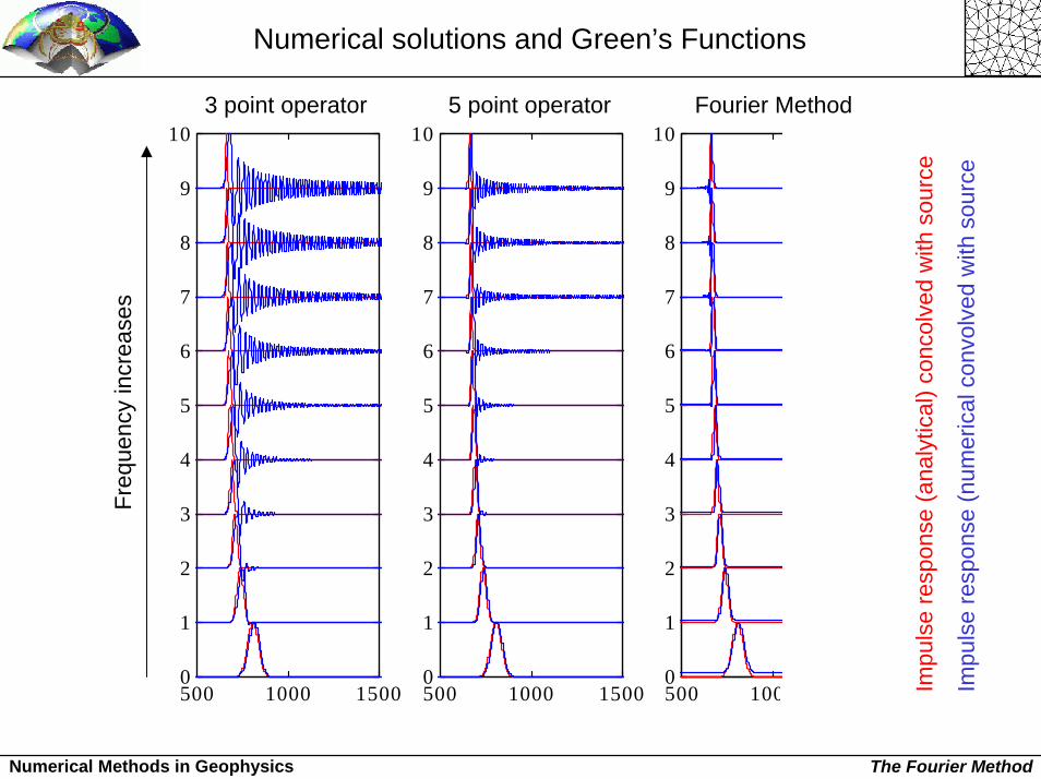
Numerical solutions and Green’s Functions

The concept of Green’s Functions (impulse responses) plays an important role in the solution of partial differential equations. It is also

useful for numerical solutions. Let us recall the acoustic wave equation

pcpt ∆=∂ 22

with ∆ being the Laplace operator. We now introduce a delta source inspace and time

pctxpt ∆+=∂ 22 )()( δδ

the formal solution to this equation is

xcxt

ctxp

)/(4

1),( 2

−=

δπ

(Full proof given in Aki and Richards, Quantitative Seismology, Freeman+Co, 1981, p. 65)



In words this means (in 1D and 3D but not in 2D, why?) , that in homogeneous media the same source time function which is input at the

source location will be recorded at a distance r, but with amplitude proportional to 1/r.

An arbitrary source can evidently be constructed by summing up different delta - solutions. Can we use this property in our numerical simulations?

What happens if we solve our numerical system with delta functions as sources?

xcxt

ctxp

)/(4

1),( 2

−=

δπ



0 200 400 600 800 10000

0.2

0.4

0.6

0.8

1

3 point operator

Source is a Delta function in space and time

0 200 400 600 800 10000

0.2

0.4

0.6

0.8

1

5 point operator

0 200 400 600 800 10000

0.2

0.4

0.6

0.8

1

Fourier Method

Impulse response (analytical)

Impulse response (numericalTime steps


500 1000 15000

1

2

3

4

5

6

7

8

9

10

500 1000

1

2

3

4

5

6

7

8

9

10

500 1000 15000

1

2

3

4

5

6

7

8

9

10



3 point operator 5 point operator Fourier MethodFr

eque

ncy

incr

ease

s

Impu

lse

resp

onse

(ana

lytic

al) c

onco

lved

with

sou

rce

Impu

lse

resp

onse

(num

eric

al c

onvo

lved

with

sou

rce

Fourier Method - Summary

The Fourier Method can be considered as the limit of the finite-difference method as the length of the operator tends to the number of points along a particular dimension.

The space derivatives are calculated in the wavenumber domain by multiplication of the spectrum with ik. The inverse Fourier transform results in an exact space derivative up to the Nyquist frequency.

The use of Fourier transform imposes some constraints on the smoothness of the functions to be differentiated. Discontinuities lead to Gibb’s phenomenon.

As the Fourier transform requires periodicity this technique is particular useful where the physical problems are periodical (e.g. angular derivatives in cylindrical problems).


- what is a pseudo-spectral method? - fourier derivatives

Documents