0 naftali tishby school of computer science and engineering hebrew university of jerusalem...
Post on 19-Dec-2015
215 views
TRANSCRIPT
1
Naftali Tishby
School of Computer Science and Engineering
Hebrew University of [email protected]
http://www.cs.huji.ac.il/~tishby
Algebraic and Information Theoretic Methods for
Network Anomaly Detection
NATO ASI School, Villa Cangola, Gazzada, Italy
2
OutlineOutline
• Statement of the problem:Statement of the problem: – Signals, observables, correlations and graphs
• Common Security Issues:Common Security Issues:– Topology:
• critical nodes, connected groups– Social:
• find his friends, how are they linked?– Temporal:
• Anomaly detection• providing warnings (predicting events)
• Algebraic methods I - static networks:Algebraic methods I - static networks:• using graph the Laplacian
• Algebraic methods II – dynamic networks:Algebraic methods II – dynamic networks:• Time dependent graphs• Diffusion on variable graphs
• Predictive Information: Predictive Information: • What in the past is predictive? • The Information Bottleneck method
6
Statement of the problem:Statement of the problem:
Signals, observables and correlations
Examples:
• Family relations• Social networks (education, joint activities,…)• Telephone calls• Sensor arrays (spatial-temporal signals)• Computer networks• ....• Neurons in the brain• Biochemical networks• General Co-Occurrence data (words-topics,…)• ….

7

8
Biological neural networks

9
Biochemical interactions
10
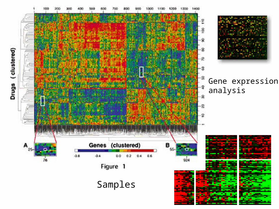
Gene expression data
• What should one measure?
Genes
Samples
Gene expressionanalysis
12
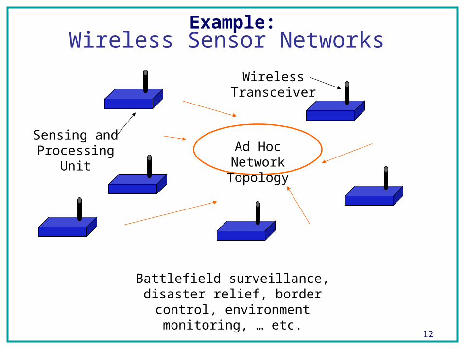
Wireless Sensor Networks
Sensing and Processing Unit
Wireless Transceiver
Ad Hoc Network Topology
Battlefield surveillance, disaster relief, border control, environment monitoring, …
etc.
Example:
13
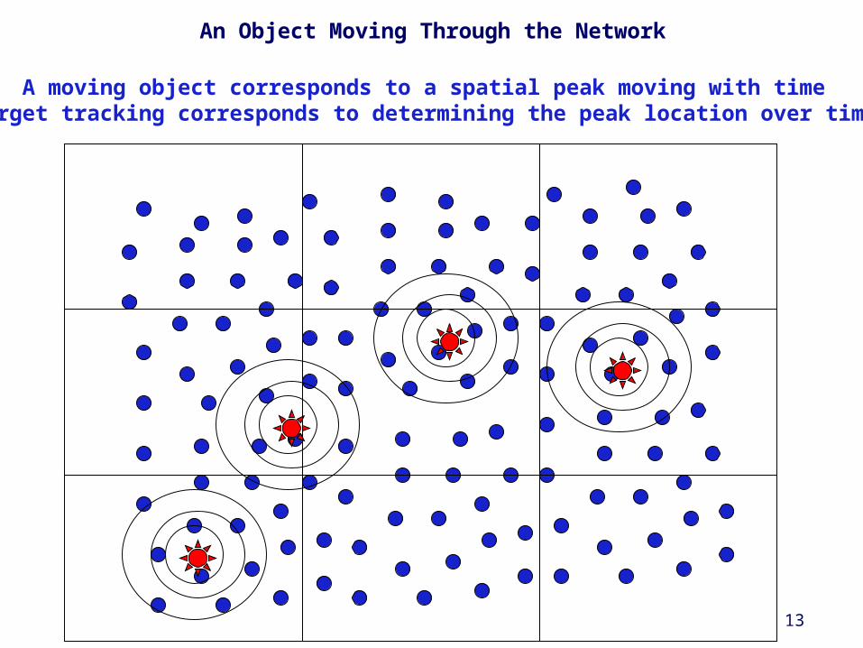
An Object Moving Through the Network
A moving object corresponds to a spatial peak moving with timeTarget tracking corresponds to determining the peak location over time

16
Graph Theoretic FormulationGraph Theoretic Formulation
• Signals, observables
Activity (charge, field) of nodes (V) in a graph• Correlations, distances, co-occurrence frequency,
Weights (current, flow) on links (E) in a graph
Graph G=(V,E) is a pair containsa vector of nodes (or vertices, V)with a matrix, W, of non-negative weights on the links (edges, E).
We first assume that the weight matrix is symmetric: Wi,j=Wj,i
i jWi,j
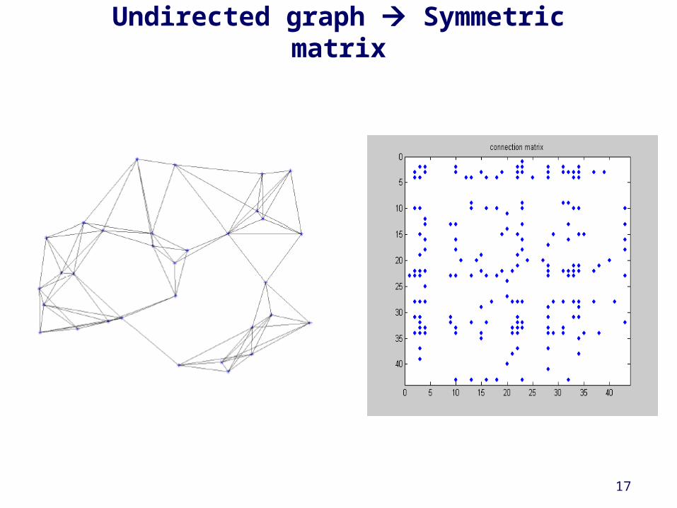
17
Undirected graph Symmetric matrix
18
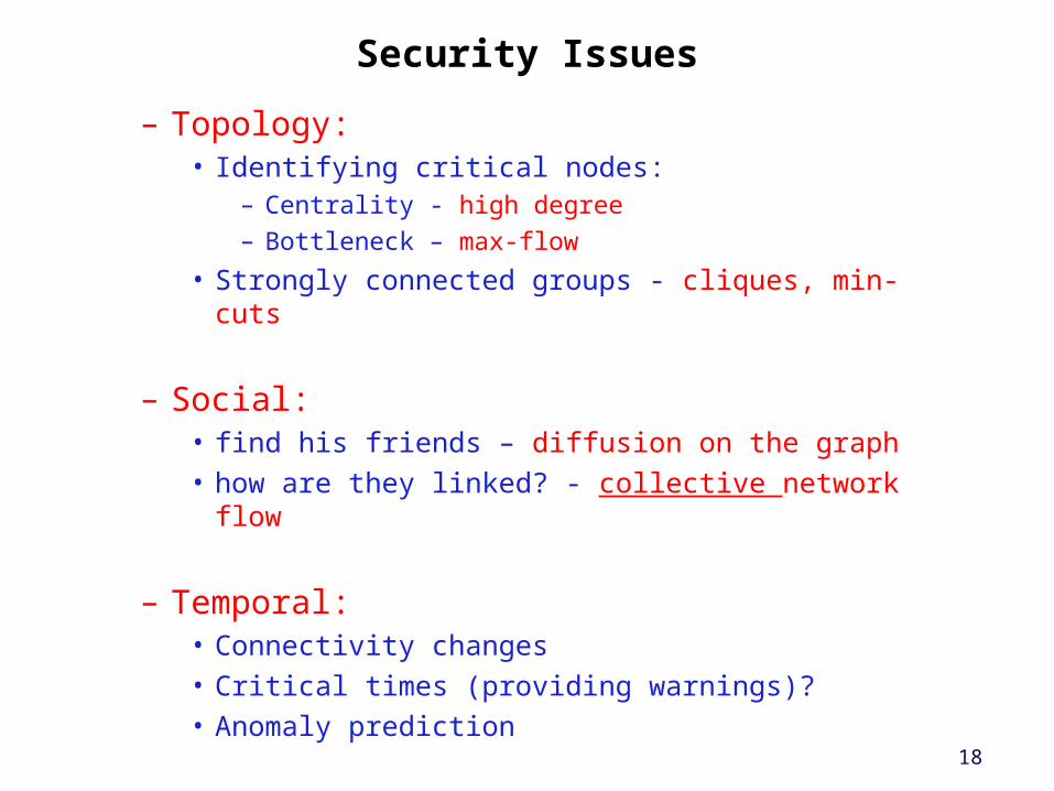
Security Issues
– Topology:• Identifying critical nodes:
– Centrality - high degree
– Bottleneck – max-flow
• Strongly connected groups - cliques, min-cuts
– Social:• find his friends – diffusion on the graph• how are they linked? - collective network flow
– Temporal:• Connectivity changes• Critical times (providing warnings)?• Anomaly prediction
19
Algebraic Methods – Static NetworksAlgebraic Methods – Static Networks
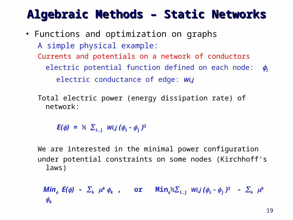
• Functions and optimization on graphsA simple physical example:Currents and potentials on a network of conductors
electric potential function defined on each node: i
electric conductance of edge: Wi,j
Total electric power (energy dissipation rate) of network:
E() = ½ i,j Wi,j (i - j )2
We are interested in the minimal power configuration
under potential constraints on some nodes (Kirchhoff's laws)
Min E() - k k k , or Min½i,j Wi,j (i - j )2 - k k k

20
Algebraic Methods – Static NetworksAlgebraic Methods – Static Networks
The quadratic energy function can be written as a quadratic form:
E() = ½i,j Wi,j (i - j )2 = ½i,j Wi,j (I2 - 2i j + j
2 )= i,j Li,j i j
Where the Graph Laplacian is defined as
L(G)=D-W
with Dj,j=i Wi,j , a diagonal matrix.
The minimum energy potential is the solution of the linear “Laplace equation” on a static graph:
L(G)=
The Lagrange multipliers are the currents through the nodes and must sum to zero. This corresponds to Kirchhoff's laws.

21
Algebraic Methods – Static Networks (cont.)Algebraic Methods – Static Networks (cont.)
Notice that L(G) is a singular matrix: the constant vector is always an eigenvector with eigenvalue 0.
In fact, the multiplicity of the zero eigenvalue, dim(ker(L)), is precisely the number of connected components of the graph!
This is the basis for important algorithms known as
“spectral graph partitioning” and “spectral clustering” (Ng, Jordan, Weiss 2000, and others):
1. Represent data-points by their Laplacian eigenvectors with low eigenvalues (spectral embedding)
2. Apply your favorite Euclidean space clustering method to this representation.

22
Laplacian eigenvector decomposition
Similar to Fourier decomposition:
• Orthogonal basis, projectors
• Eigenvalues – spatial frequencies
L(G) xk = k xk
X1 X2 X3 …

23
Application: Using Spectral Embedding Application: Using Spectral Embedding for Novelty Detection in for Novelty Detection in communication networkscommunication networks
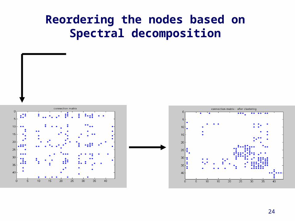
1. Represent the connection matrix using its Laplacian eigenvector decomposition
2. Filter the high frequency (small) components to remain with the large connected blocks
3. Use the filtered connections as a reference and measure the distance of current graph to the reference.
24
Reordering the nodes based on Spectral decomposition

26
Simple illustration

27
Distances between graphs
• Since graphs are represented by weight matrices we can use any matrix norm to measure graph similarity
• We can expand the Laplacian in its eigenvectors:
• Where pi is a projection on the i-th eigenvector
a projection on first K eigenvectors – a low-pass filter!
1 1
( )N N
Ti i i i i
i i
L G x x p
1 1[ ,..., ][ ,..., ]T TK K K K KP E E x x x x
28
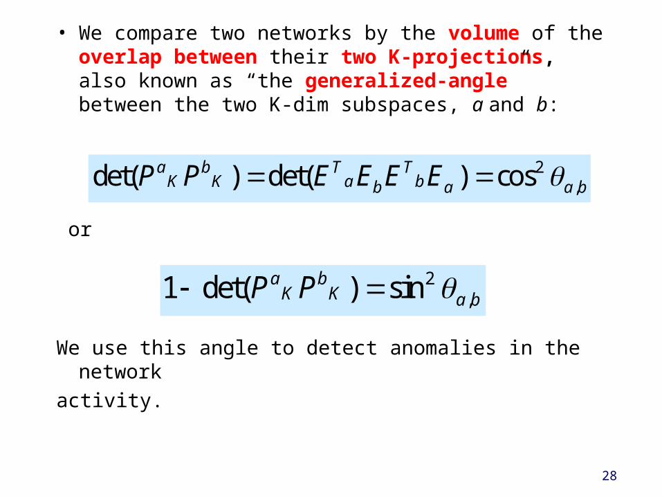
• We compare two networks by the volume of the overlap between their two K-projections, also known as “the generalized-angle” between the two K-dim subspaces, a and b:
or
We use this angle to detect anomalies in the network
activity.
2,det( ) det( ) cosa b T T
K K a bb a a bP P E E E E
2,1 det( ) sina b
K K a bP P

29
30
31
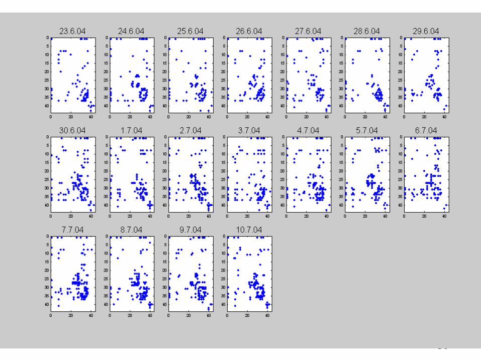
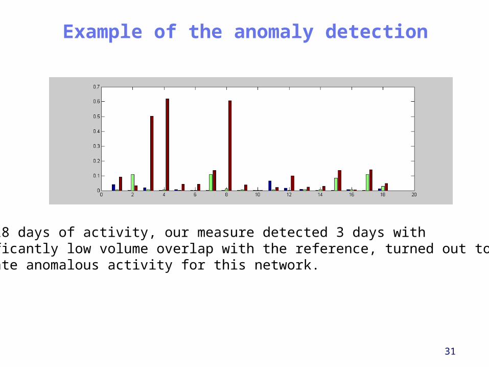
Example of the anomaly detection
over 18 days of activity, our measure detected 3 days withsignificantly low volume overlap with the reference, turned out to truly Indicate anomalous activity for this network.

38
Diffusion on Graphs
The next question: who is connected with whom?
This can be modeled as a spread of a disease through a population, a forest fire, or ink on paper… through “diffusion”
The graph Laplacian is also the generator for random walks on the graph, or diffusion.
Denoting by the density on the node x at time t,then the diffusion equation on the graph:
is a linear differential equation, which is solved by the matrix exponential:
39
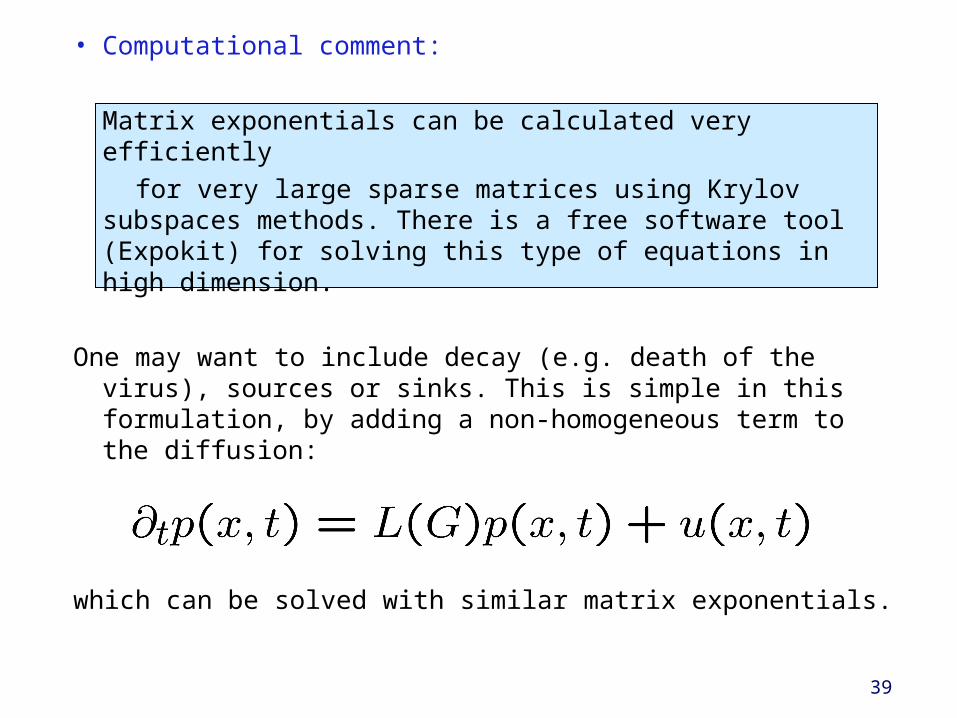
• Computational comment:
Matrix exponentials can be calculated very efficiently
for very large sparse matrices using Krylov subspaces methods. There is a free software tool (Expokit) for solving this type of equations in high dimension.
One may want to include decay (e.g. death of the virus), sources or sinks. This is simple in this formulation, by adding a non-homogeneous term to the diffusion:
which can be solved with similar matrix exponentials.
40
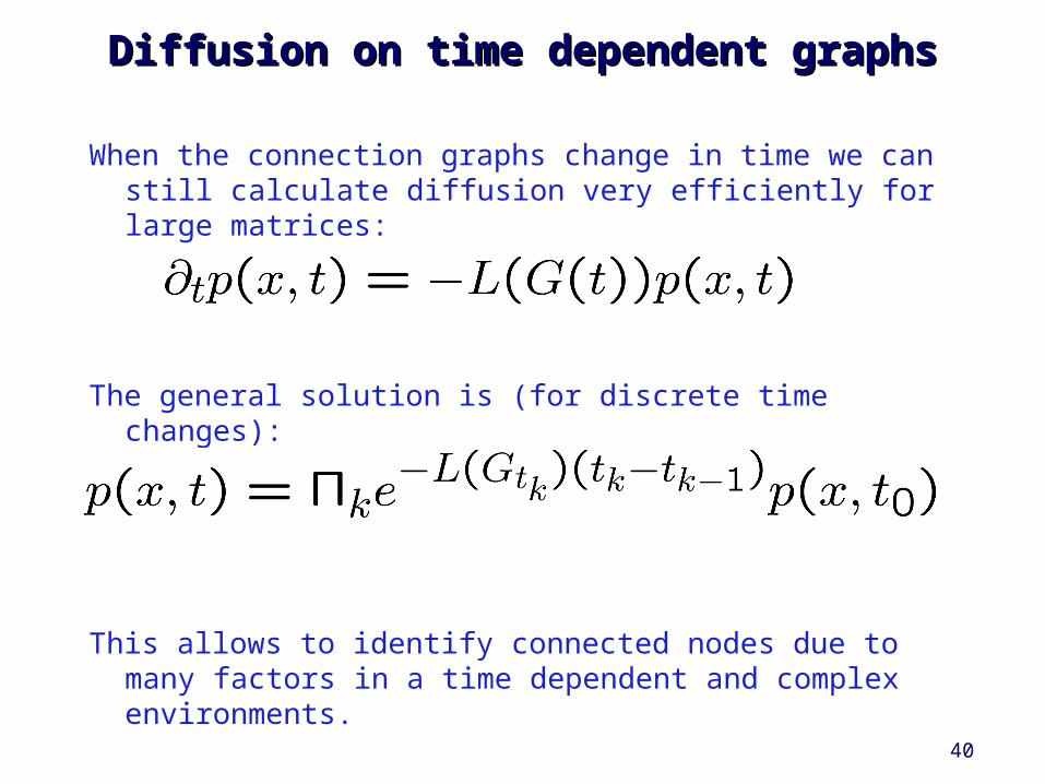
Diffusion on time dependent graphsDiffusion on time dependent graphs
When the connection graphs change in time we can still calculate diffusion very efficiently for large matrices:
The general solution is (for discrete time changes):
This allows to identify connected nodes due to many factors in a time dependent and complex environments.

41
Predictive InformationPredictive Information
– What in the past is predictive? • Predictive information is sub-exponential!• Finding predictive statistics • Prediction suffix trees
– The Information Bottleneck method:– Extracting relevant statistics from large data
42
Why Predictability?
• X1, X2,… Xn,….
• time series extrapolation isdifferent than prediction
• Prediction is Probabilistic

43
Why Predictability? Life is all about predictions…
44
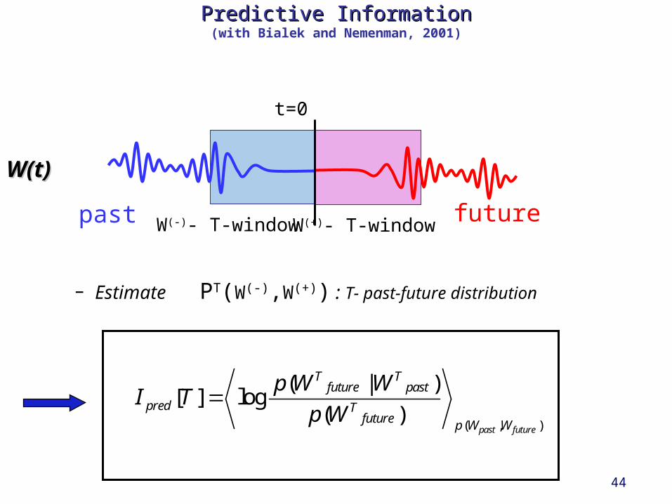
Predictive InformationPredictive Information(with Bialek and Nemenman, 2001)
– Estimate PT(W(-),W(+)) : T- past-future distribution
W(t)W(t)
past futureW(-)- T-window
t=0
W(+)- T-window
( , )
( | )[ ] log
( )past future
T Tfuture past
pred Tfuture p W W
p W WI T
p W
45
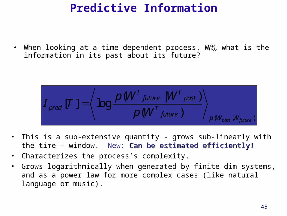
Predictive Information
• When looking at a time dependent process, W(t), what is the information in its past about its future?
• This is a sub-extensive quantity - grows sub-linearly with the time - window. New: Can be estimated efficiently!Can be estimated efficiently!
• Characterizes the process’s complexity. • Grows logarithmically when generated by finite dim systems, and as a
power law for more complex cases (like natural language or music).
( , )
( | )[ ] log
( )past future
T Tfuture past
pred Tfuture p W W
p W WI T
p W

46
Logarithmic growth for finite dimensional processes
• Finite parameter processes (e.g. Markov chains)
• Similar to stochastic complexity (MDL)
dim( )( ) log
2predI T T

47
Power law growth
• Such fast growth is a signature of infinite dimensional processes
• Power laws emerges in cases where the interactions/correlations have long range
( ) 1predI T T

48
Entropy of words in a Spin Chain
12
02 )(log)()(
N
kKNKN WPWPNS

49
Entropy of 3 Generated Chains
total.spins 10 · 1
spins 400000every
)j-i
1 (0,Νfrom
randomat taken is J •
spins 400000every
1) N(0, from randomat
takenis J , J J •
J •
9
ij
01ji,0ij
1ji,ij
Entropy is Extensive : it shows No distinction between the cases!

50
Predictive Information –Subextensive Component of the Entropy
shows a qualitative distinction between the cases!
Subextensive component growth is
reflecting the underlying complexity!

51
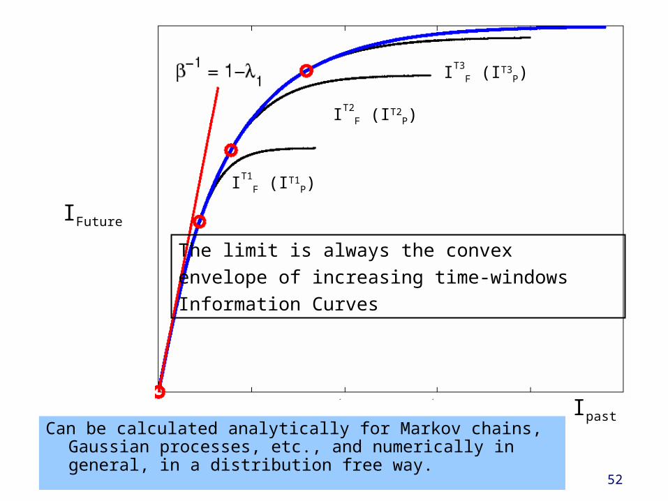
– Using the Information Bottleneck method:Solve:
MinZ I(W(-);Z) - I(W(+);Z) for all >0
T- past-future information curve: ITF(ITP)
– IFuture(IPast) = limT! 1 ITF(ITP)
But WHAT - in the past - is predictive ?But WHAT - in the past - is predictive ?
W(t)W(t)
past futureW(-)- T-window
t=0
W(+)- T-window
52
Can be calculated analytically for Markov chains, Gaussian processes, etc., and numerically in general, in a distribution free way.
IFuture
Ipast
IT1F (IT1
P)
IT2F (IT2
P)
IT3F (IT3
P)
The limit is always the convexenvelope of increasing time-windowsInformation Curves

53
The Information Bottleneck Method
N. Tishby, F.C. Pereira and W. Bialek, 1999.
54
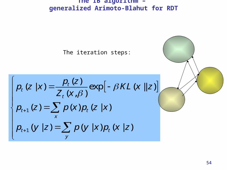
The IB algorithm – generalized Arimoto-Blahut for RDT
The iteration steps:
1
1
( )( | ) exp ( || )
( , )
( ) ( ) ( | )
( | ) ( | ) ( | )
tt
t
t tx
t ty
p zp z x KL x z
Z x
p z p x p z x
p y z p y x p x z
55
Why is the predictive information interesting?Why is the predictive information interesting?
It determines the level of adaptation of It determines the level of adaptation of organisms to stochastic environments…organisms to stochastic environments…
Interesting Key example: Human Languages

56
Variable Memory Markov Modelsand Prediction Suffix Tree Learning
[Ron, Singer, Tishby, 1995,96]
• Can be learned accurately and efficiently• Can capture high-order correlations (better than HMM)• Effectively “capture” short “features” and “motifs”

57
Complexity
Acc
ura
cy
Possible Models/representations
Limited dataLimited data
Bounded Bounded
ComputationComputation
Complexity – Accuracy Tradeoff
58
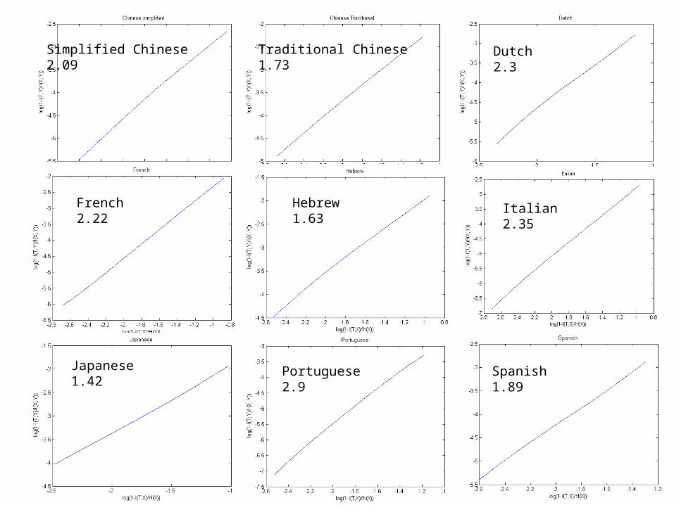
Simplified Chinese2.09
Traditional Chinese1.73
Dutch2.3
French2.22
Hebrew1.63
Italian2.35
Japanese1.42
Portuguese2.9
Spanish1.89
59
0 0.1 0.2 0.3 0.4 0.5 0.6 0.7 0.8 0.9 10
0.1
0.2
0.3
0.4
0.5
0.6
0.7
0.8
0.9
1
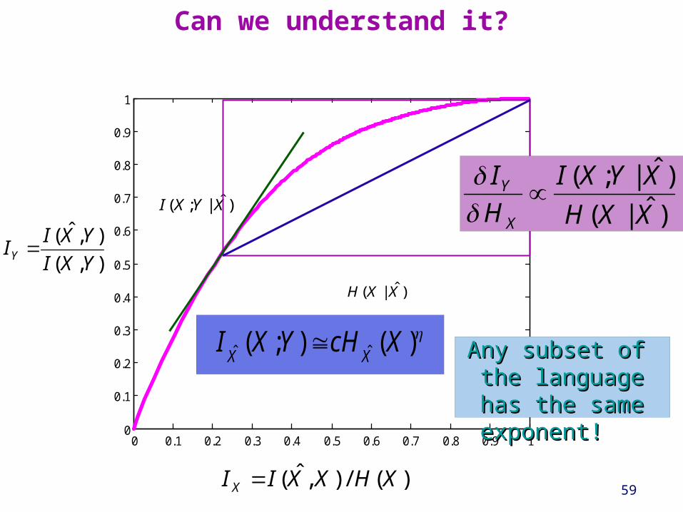
)();( ˆˆ XcHYXIXX
Can we understand it?
)ˆ|;( XYXI
),(
),ˆ(
YXI
YXIIY
)(/),ˆ( XHXXII X
)ˆ|(
)ˆ|;(
XXH
XYXI
H
I
X
Y
Any subset of Any subset of the language the language has the same has the same exponent! exponent!
)ˆ|( XXH

60
Many Thanks to…Many Thanks to…
• Bill BialekBill Bialek• Ilya NemenmanIlya Nemenman• Naama Parush Naama Parush • Jonathan RubinJonathan Rubin• Eli NelkenEli Nelken• Dmitry DavidovDmitry Davidov• Felix Creutzig Felix Creutzig • Amir GlobersonAmir Globerson• Gal Chechik Gal Chechik • Roi WeissRoi Weiss