q0

q1

q3

q1

q2

q1

q4

start 0

1

0

1

0, 1

ℒ(M) = ((0|1)ℒ *(00|11))

Mathematical Foundations of Computing

CS103CS103Preliminary Course Notes

Keith Schwarz

Fall 2012

Table of Contents

Chapter 0   Introduction  5  0.1 How These Notes are Organized   5  0.2 Acknowledgements   7  

Chapter 1   Sets and Cantor's Theorem  9  1.1 What is a Set?   9  1.2 Operations on Sets   11  1.3 Special Sets   15  1.4 Set­Builder Notation   17  

Filtering Sets   17  Transforming Sets   19  

1.5 Relations on Sets   20  Set Equality   20  Subsets and Supersets   21  

The Empty Set and Vacuous Truths   22  1.6 The Power Set   23  1.7 Cardinality   25  

What is Cardinality?   25  The Difficulty With Infinite Cardinalities   27  A Formal Definition of Cardinality   28  

1.8 Cantor's Theorem   32  How Large is the Power Set?   33  Cantor's Diagonal Argument   34  Formalizing the Diagonal Argument   37  Proving Cantor's Theorem   39  

1.9 Why Cantor's Theorem Matters   40  1.10 The Limits of Computation   41  

What Does This Mean?   42  1.11 Chapter Summary   43  

Chapter 2   Mathematical Proof  45  2.1 What is a Proof?   45  

What Can We Assume?   46  2.2 Direct Proofs   46  

Proof by Cases   49  A Quick Aside: Choosing Letters   51  

Proofs about Sets   51  Lemmas   55  Proofs with Vacuous Truths   59  

2.3 Indirect Proofs   60  Logical Implication   61  Proof by Contradiction   62  Rational and Irrational Numbers   66  Proof by Contrapositive   68  

2.4 Chapter Summary   72  2.5 Chapter Exercises   72  

Chapter 3   Mathematical Induction  75  3.1 The Principle of Mathematical Induction   75  

The Flipping Glasses Puzzle   76  3.2 Summations   81  

Summation Notation   87  Summing Odd Numbers   90  Manipulating Summations   95  Telescoping Series   100  Products   106  

3.3 Induction and Recursion   107  Monoids and Folds     113  ★

3.4 Variants on Induction   116  Starting Induction Later   116  Fibonacci Induction   123  

Climbing Down Stairs   125  Computing Fibonacci Numbers   129  

3.5 Strong Induction   134  The Unstacking Game   138  Variations on Strong Induction   148  A Foray into Number Theory     153  ★Why Strong Induction Works   162  

3.6 The Well­Ordering Principle   164  Proof by Infinite Descent   164  Proving the Well­Ordering Principle   168  

An Incorrect Proof   168  A Correct Proof   170  

3.7 Chapter Summary   171  3.8 Chapter Exercises   171  

Chapter 4   Graph Theory  177  4.1 Basic Definitions   178  

Ordered and Unordered Pairs   178  A Formal Definition of Graphs   179  Navigating a Graph   181  

4.2 Graph Connectivity   183  Connected Components   184  2­Edge­Connected Graphs   192  Trees   201  

Properties of Trees   210  Directed Connectivity   219  

4.3 DAGs   224  Topological Orderings   227  Condensations   235  

4.4 Matchings   242  Proving Berge's Theorem     250  ★

4.5 Chapter Summary   261  4.6 Chapter Exercises   262  

Chapter 5   Relations  267  5.1 Basic Terminology   267  

Tuples and the Cartesian Product   267  Cartesian Powers   270  

A Formal Definition of Relations   271  Special Binary Relations   274  Binary Relations and Graphs   277  

5.2 Equivalence Relations   282  Equivalence Classes   283  Equivalence Classes and Graph Connectivity   292  

5.3 Order Relations   293  Strict Orders   293  Partial Orders   297  Hasse Diagrams   303  Preorders   309  

Properties of Preorders   310  Combining Orderings   316  

The Product Ordering   317  The Lexicographical Ordering   319  

5.4 Well­Ordered and Well­Founded Sets   324  Well­Orders   325  

Properties of Well­Ordered Sets   326  Well­Founded Orders   329  Well­Ordered and Well­Founded Induction     331  ★

Application: The Ackermann Function   335  5.5 Chapter Summary   339  5.6 Chapter Exercises   340  

Chapter 0 IntroductionComputer science is the art of solving problems with computers. This is a broad definition that encompasses an equally broad field. Within computer science, we find software engineering, bioinformatics, cryptography, machine learning, human-computer interaction, graphics, and a host of other fields.

Mathematics underpins all of these endeavors in computer science. We use graphs to model complex problems, and exploit their mathematical properties to solve them. We use recursion to break down seemingly insurmountable problems into smaller and more manageable problems. We use topology, linear algebra, and geometry in 3D graphics. We study computation itself in computability and complexity theory, with results that have profound impacts on compiler de-sign, machine learning, cryptography, computer graphics, and data processing.

This set of course notes serves as a first course in the mathematical foundations of computing. It will teach you how to model problems mathematically, reason about them abstractly, and then apply a battery of techniques to explore their properties. It will teach you to prove mathematical truths beyond a shadow of a doubt. It will give you insight into the fundamental nature of com-putation and what can and cannot be solved by computers. It will introduce you to complexity theory and some of the most important problems in all computer science.

This set of course notes is intended to give a broad and deep introduction to the mathematics that lie at the heart of computer science. It begins with a survey of discrete mathematics – basic set theory and proof techniques, mathematic induction, graphs, relations, functions, and logic – then explores computability and complexity theory. No prior mathematical background is necessary.

These course notes are designed to provide a secondary treatment of the material from Stanford's CS103 course. The topic organization roughly follows the presentation from CS103, albeit at a much deeper level. It is designed to supplement lectures from CS103 with additional exposition on each topic, broader examples, and more advanced applications and techniques. My hope is that there will be something for everyone. If you're interested in brushing up on definitions and seeing a few examples of the various techniques, feel free to read over the relevant parts of each chapter. If you want to see the techniques applied to a variety of problems, look over the exam-ples that catch your interest. If you want to see just how deep the rabbit hole goes, read over the entire chapter and work through all the starred exercises.

0.1 How These Notes are OrganizedThe organization of this book into chapters is as follows:

• Chapter One motivates our discussion of mathematics by giving a brief outline of set the-ory, concluding with Cantor's theorem, a profound and powerful result about the nature of infinity.

• Chapter Two lays the groundwork for formal proofs by exploring several key proof tech-niques that we will use throughout the rest of these notes.

• Chapter Three explores mathematical induction, a proof technique that we will use exten-sively when proving results about discrete structures, programs, and computation.

• Chapter Four investigates mathematical structures called graphs that are useful for mod-eling complex problems. These structures will form the basis for many of the models of computation we will investigate later.

• Chapter Five explores different ways in which objects often relate to one another and the mathematical structures of these relations.

• Chapter Six revisits the material on set theory from the first chapter with a mathemati-cally rigorous exploration of the properties of infinity.

• Chapter Seven introduces a proof technique called the pigeonhole principle that superfi-cially appears quite simple, but which has profound implications for the limits of compu-tation.

• Chapter Eight explores formal logic and gives a more rigorous basis for the proof tech-niques developed in the preceding chapters.

• Chapter Nine introduces key concepts from computability theory, the study of what prob-lems can and cannot be solved by a computer.

• Chapter Ten introduces finite automata, regular expressions, and the regular languages. It serves as an introduction to the study of formal models of computations. These models have applications throughout computer science

• Chapter Eleven introduces pushdown automata and context-free grammars, more power-ful formalisms for describing computation.

• Chapter Twelve introduces the Turing machine, an even more powerful model of compu-tation that we suspect is the most powerful feasible computing machine that could ever be built.

• Chapter Thirteen explores the power of the Turing machine by exploring what problems it can solve.

• Chapter Fourteen provides examples of problems that are provably beyond our capability to solve with any type of computer.

• Chapter Fifteen introduces reductions, a fundamental technique in computability and complexity theory for reasoning about the relative difficulties of problems.

• Chapter Sixteen introduces complexity theory, the study of what problems can be com-puted given various resource constraints.

• Chapter Seventeen introduces the complexity classes P and NP, which contain many problems of great practical and theoretical importance.

• Chapter Eighteen explores the connection between the classes P and NP, which (as of 2012) is the single biggest open problem in all of theoretical computer science.

• Chapter Nineteen goes beyond P and NP and explores alternative models of computation and their complexities.

• Chapter Twenty concludes our treatment of the mathematical foundations of computing and sets the stage for further study on the subject.

Some of the sections of these notes are marked with a symbol. These sections contain more★ advanced material that, while interesting, is not essential to understanding the course material. If you are interested in learning more about the topic, I would suggest reading through it. How-ever, if you're pressed for time, feel free to skip these sections.

Similarly, some of the chapter exercises are marked with the symbol. These exercises are★ more difficult than the other exercises. I highly recommend attempting at least one or two of the starred exercises from each chapter. If you're up for a real challenge, try working through all of them!

This is a work-in-progress draft of what I hope will become a full set of course notes for CS103. Right now, the notes only cover up through the first six or seven lectures. I am hoping to expand that over the course of the upcoming months. Since this is a first draft, there are definitely going to be errors in here, whether they're typoz, grammatically problems, layout

issues, and logic errors. If you find any errors, please don't hesitate to get in touch with me at htiek@cs.stanford.edu – I genuinely want these notes to be as good as they can be, so any feedback would be most appreci-ated.

0.2 AcknowledgementsThese course notes represent the product of six months of hard work. I received invaluable feed-back on the content and structure from many of my friends, students, and colleagues. In particu-lar, I'd like to thank Leonid Shamis, Sophia Westwood, and Amy Nguyen for their comments. Their feedback has dramatically improved the quality of these notes, and I'm very grateful for the time and effort they put into reviewing drafts at every stage.

Chapter 1 Sets and Cantor's TheoremOur journey into the realm of mathematics begins with an exploration of a surprisingly nuanced concept: the set. Informally, a set is just a collection of things, whether it's a set of numbers, a set of clothes, a set of nodes in a network, or a set of other sets. Amazingly, given this very simple starting point, it is possible to prove a result known as Cantor's Theorem that provides a striking and profound limit on what problems a computer program can solve. In this introductory chap-ter, we'll build up some basic mathematical machinery around sets, then will see how the simple notion of asking how big a set is can lead to incredible and shocking results.

1.1 What is a Set?Let's begin with a simple definition:

A set is an unordered collection of distinct elements.

What exactly does this mean? Intuitively, you can think of a set as a group of things. Those things must be distinct, which means that you can't have multiple copies of the same object in a set. Additionally, those things are unordered, so there's no notion of a “first” thing in the group, a “second” thing in a group, etc.

We need two additional pieces of terminology to talk about sets:

An element is something contained within a set.

To denote a set, we write the elements of the set within curly braces. For example, the set {1, 2, 3} is a set with three elements: 1, 2, and 3. The set { cat, dog } is a set containing the two ele-ments “cat” and “dog.”

Because sets are unordered collections, the order in which we list the elements of a set doesn't matter. This means that the sets {1, 2, 3}, {2, 1, 3}, and {3, 2, 1} are all descriptions of exactly the same set. Also, because sets are unordered collections of distinct elements, no element can appear more than once in the same set. In particular, this means that if we write out a set like {1, 1, 1, 1, 1}, it's completely equivalent to writing out the set {1}, since sets can't contain dupli -cates. Similarly, {1, 2, 2, 2, 3} and {3, 2, 1} are the same set, since ordering doesn't matter and duplicates are ignored.

When working with sets, we are often interested in determining whether or not some object is an element of a set. We use the notation x ∈ S to denote that x is an element of the set S. For exam-ple, we would write that 1 {1, 2, 3}, or that cat { cat, dog }. If spoken aloud, you'd read∈ ∈ x ∈ S as “x is an element of S.” Similarly, we use the notation x ∉ S to denote that x is not an el-ement of S. So, we would have 1 {2, 3, 4}, dog {1, 2, 3}, and ibex {cat, dog}. You can∉ ∉ ∉ read x ∉ S as “x is not an element of S.”

Chapter 1: Sets and Cantor's Theorem

Sets appear almost everywhere in mathematics because they capture the very simple notion of a group of things. If you'll notice, there aren't any requirements about what can be in a set. You can have sets of integers, set of real numbers, sets of lines, sets of programs, and even sets of other sets. Through the remainder of your mathematical career, you'll see sets used as building blocks for larger and more complicated objects.

As we just mentioned, it's possible to have sets that contain other sets. For example, the set { {1, 2}, 3 } is a set containing two elements – the set {1, 2} and the number 3. There's no re -quirement that all of the elements of a set have the same “type,” so a single set could contain numbers, animals, colors, and other sets without worry. That said, when working with sets that contain other sets, it's important to note what the elements of that set are. For example, consider the set

{{1, 2}, {2, 3}, 4}

has just three elements: {1, 2}, {2, 3}, and 4. This means that

{1, 2} {{1, 2}, {2, 3}, 4}∈

{2, 3} {{1, 2}, {2, 3}, 4}∈

4 {{1, 2}, {2, 3}, 4}∈

However, it is not true that 1 {{1, 2}, {2, 3}, 4}. Although {{1, 2}, {2, 3}, 4} contains the set∈ {1, 2} which in turn contains 1, 1 itself is not an element of {{1, 2}, {2, 3}, 4}. In a sense, set containment is “opaque,” in that it just asks whether the given object is directly contained within the set, not whether it is contained with that set, a set contained within that set, etc. Conse-quently, we have that

1 {{1, 2}, {2, 3}, 4}∉

2 {{1, 2}, {2, 3}, 4}∉

3 {{1, 2}, {2, 3}, 4}∉

But we do have that

4 {{1, 2}, {2, 3}, 4}∈

Because 4 is explicitly listed as a member of the set.

In the above example, it's fairly time-consuming to keep writing out the set {{1, 2}, {2, 3}, 4} over and over again. Commonly, we'll assign names to mathematical objects to make it easier to refer to them in the future. In our case, let's call this set “S.” Mathematically, we can write this out as

S = {{1, 2}, {2, 3}, 4}

Given this definition, we can rewrite all of the above discussion much more compactly:

{1, 2} ∈ S

{2, 3} ∈ S

4 ∈ S

1 ∉ S

2 ∉ S

3 ∉ S

11 / 347

Throughout this book, and in the mathematical world at large, we'll be giving names to things and then manipulating and referencing those objects through those names. Hopefully you've used variables before when programming, so I hope that this doesn't come as too much of a sur-prise.

Before we move on and begin talking about what sorts of operations we can perform on sets, we need to introduce a very special set that we'll be making extensive use of: the empty set.

The empty set is the set that does not contain any elements.

It may seem a bit strange to think about a collection of no things, but that's precisely what the empty set is. You can think of the empty set as representing a group that doesn't have anything in it. One way that we could write the empty set is as { }, indicating that it's a set (the curly braces), but that this set doesn't contain anything (the fact that there's nothing in-between them!) However, in practice this notation is not used, and we use the special symbol Ø to denote the empty set.

The empty set has the nice property that there's nothing in it, which means that for any object x that you ever find anywhere, x Ø. This means that the statement x Ø is always false.∉ ∈

Let's return to our earlier discussion of sets containing other sets. It's possible to build sets that contain the empty set. For example, the set { Ø } is a set with one element in it, which is the empty set. Thus we have that Ø { Ø }. More importantly, note that Ø and { Ø } are ∈ not the same set. Ø is a set that contains no elements, while { Ø } is a set that does indeed contain an el-ement, namely the empty set. Be sure that you understand this distinction!

1.2 Operations on SetsSets represent collections of things, and it's common to take multiple collections and ask ques-tions of them. What do the collections have in common? What do they have collectively? What does one set have that the other does not? These questions are so important that mathematicians have rigorously defined them and given them fancy mathematical names.

First, let's think about finding the elements in common between two sets. Suppose that I have two sets, one of US coins and one of chemical elements. This first set, which we'll call C, is

C = { penny, nickel, dime, quarter, half-dollar, dollar }

and the second set, which we'll call E, contains these elements:

E = { hydrogen, helium, lithium, beryllium, boron, carbon, …, ununseptium }

(Note the use of the ellipsis here. It's often acceptable in mathematics to use ellipses when there's a clear pattern present, as in the above case where we're listing the elements in order. Usually, though, we'll invent some new symbols we can use to more precisely describe what we mean.)

The sets C and E happen to have one element in common: nickel, since

nickel ∈ C

Chapter 1: Sets and Cantor's Theorem

and

nickel ∈ E

However, some sets may have a larger overlap. For example, consider the sets {1, 2, 3} and {1, 3, 5}. These sets have both 1 and 3 in common. Other sets, on the other hand, might not have anything in common at all. For example, the sets {cat, dog, ibex} and {1, 2, 3} have no elements in common.

Since sets serve to capture the notion of a collection of things, we might think about the set of el-ements that two sets have in common. In fact, that's a perfectly reasonable thing to do, and it goes by the name intersection:

The intersection of two sets S and T, denoted S ∩ T, is the set of elements contained in both S and T.

For example, {1, 2, 3} ∩ {1, 3, 5} = {1, 3}, since the two sets have exactly 1 and 3 in common. Using the set C of currency and E of chemical elements from earlier, we would say that C ∩ E = {nickel}.

But what about the intersection of two sets that have nothing in common? This isn't anything to worry about. Let's take an example: what is {cat, dog, ibex} ∩ {1, 2, 3}? If we consider the set of elements common to both sets, we get the empty set Ø, since there aren't any common ele-ments between the two sets.

Graphically, we can visualize the intersection of two sets by using a Venn diagram, a pictorial representation of two sets and how they overlap. You have probably encountered Venn diagrams before in popular media. These diagrams represent two sets as overlapping circles, with the ele-ments common to both sets represented in the overlap. For example, if A = {1, 2, 3} and B = {3, 4, 5}, then we would visualize the sets as

A B

1

2

4

5

3

Given a Venn diagram like this, the intersection A ∩ B is the set of elements in the intersection, which in this case is {3}.

Just as we may be curious about the elements two sets have in common, we may also want to ask what elements two sets contain collectively. For example, given the sets A and B from above, we can see that, collectively, the two sets contain 1, 2, 3, 4, and 5. Mathematically, the set of ele-ments held collectively by two sets is called the union:

13 / 347

The union of two sets A and B, denoted A ∪ B, is the set of all elements contained in ei-ther of the two sets.

Thus we would have that {1, 2, 3} {∪ 3, 4, 5} = {1, 2, 3, 4, 5} (here, I'm color-coding the num-bers to indicate which sets they're from; we'll treat all numbers as the same regardless of their color). Note that, since sets are unordered collections of distinct elements, that it would also have been correct to write {1, 2, 3, 3, 4, 5} as the union of the two sets, since {1, 2, 3, 4, 5} and {1, 2, 3, 3, 4, 5} describe the same set. That said, to eliminate redundancy, typically we'd prefer to write out {1, 2, 3, 4, 5} since it gets the same message across in smaller space.

The symbols for union ( ) and intersection (∩) are similar to one another, and it's often easy to∪ get them confused. A useful mnemonic is that the symbol for union looks like a U, so you can think of the nion of two sets.∪

An important (but slightly pedantic) point is that can only be applied to two sets. This means∪ that although

{1, 2, 3} 4∪

might intuitively be the set {1, 2, 3, 4}, mathematically this statement isn't meaningful because 4 isn't a set. If we wanted to represent the set formed by taking the set {1, 2, 3} and adding 4 to it, we would represent it by writing

{1, 2, 3} {4}∪

Now, since both of the operands are sets, the above expression is perfectly well-defined. Simi-larly, it's not mathematically well-defined to say

{1, 2, 3} ∩ 3

because 3 is not a set. Instead, we should write

{1, 2, 3} ∩ {3}

Another important point to clarify when working with union or intersection is how they behave when applied to sets containing other sets. For example, what is the value of the following ex-pression?

{{1, 2}, {3}, {4}} ∩ {{1, 2, 3}, {4}}

When computing the intersection of two sets, all that we care about is what elements the two sets have in common. Whether those elements themselves are sets or not is irrelevant. Here, for ex-ample, we can list off the elements of the two sets {{1, 2}, {3}, {4}} and {{1, 2, 3}, {4}} as fol-lows:

{1, 2} {{1, 2}, {3}, {4}}∈ {1, 2, 3} {{1, 2, 3}, {4}}∈

{3} {{1, 2}, {3}, {4}}∈ {4} {{1, 2, 3}, {4}}∈

{4} {{1, 2, 3}, {4}}∈

Looking at these two lists of elements, we can see that the only element that the two sets have in common is the element {4}. As a result, we have that

Chapter 1: Sets and Cantor's Theorem

{{1, 2}, {3}, {4}} ∩ {{1, 2, 3}, {4}} = {{4}}

That is, the set of just one element, which is the set containing 4.

You can think about computing the intersection of two sets as the act of peeling off just the outer-most braces from the two sets, leaving all the elements undisturbed. Then, looking at just those elements, find the ones in common to both sets, and gather all of those elements back together.

The union of two sets works similarly. So, if we want to compute

{{1, 2}, {3}, {4}} {{1, 2, 3}, {4}}∪

We would “peel off” the outer braces to find that the first set contains {1, 2}, {3}, and {4} and that the second set contains {1, 2, 3} and {4}. If we then gather all of these together into a set, we get the result that

{{1, 2}, {3}, {4}} {{1, 2, 3}, {4}} = {{1, 2}, {3}, {1, 2, 3}, {4}}∪

Given two sets, we can find what they have in common by finding their intersection and can find what they have collectively by using the union. But both of these operations are symmetric; it doesn't really matter what order the sets are in, since A ∪ B = B ∪ A and A ∩ B = B ∩ A. (If this doesn't seem obvious, try out a couple of examples and see if you notice anything). In a sense, the union and intersection of two sets don't have a “privileged” set. However, at times we might be interested in learning about how one set differs from another. Suppose that we have two sets A and B and want to find the elements of A that don't appear in B. For example, given the sets A = {1, 2, 3} and B = {3, 4, 5}, we would note that the elements 1 and 2 are unique to A and don't appear anywhere in B, and that 4 and 5 are unique to B and don't appear in A. We can cap-ture this notion precisely with the set difference operation:

The set difference of A and B, denoted A – B or A \ B, is the set of elements contained in A but not contained in B.

Note that there are two different notations for set difference. In this book we'll use the minus sign to indicate set subtraction, but other authors use the slash for this purpose. You should be comfortable working with both.

As an example of a set difference, {1, 2, 3} – {3, 4, 5} = {1, 2}, because 1 and 2 are in {1, 2, 3} but not {3, 4, 5}. Note, however, that {3, 4, 5} – {1, 2, 3} = {4, 5}, because 4 and 5 are in {3, 4, 5} but not {1, 2, 3}. Set difference is not symmetric. It's also possible for the difference of two sets to contain nothing at all, which would happen if everything in the first set is also con-tained in the second set. For instance, {1, 2, 3} – {1, 2, 3, 4} = Ø, since every element of{1, 2, 3} is also contained in {1, 2, 3, 4}.

There is one final set operation that we will touch on for now. Suppose that you and I travel the world and each maintain a set of the places that we went. If we meet up to talk about our trip, we'd probably be most interested to tell each other about the places that one of us had gone but the other hadn't. Let's say that set A is the set of places I have been and set B is the set of places that you've been. If we take the set A – B, this would give the set of places that I have been that you hadn't, and if you take the set B – A it would give the set of places that you have been that I hadn't. These two sets, taken together, are quite interesting, because they represent fun places to

15 / 347

talk about, since one of us would always be interested in hearing what the other had to say. Us-ing just the operators we've talked about so far, we could describe this set as(B – A) (∪ A – B). For simplicity, though, we usually define one final operation on sets that makes this concept easier to convey: the symmetric difference.

The set symmetric difference of two sets A and B, denoted A Δ B, is the set of elements that are contained in exactly one of A or B, but not both.

For example, {1, 2, 3} Δ {3, 4, 5} = {1, 2, 4, 5}, since 1 and 2 are in {1, 2, 3} but not {3, 4, 5} and 4 and 5 are in {3, 4, 5} but not {1, 2, 3}.

1.3 Special SetsSo far, we have described sets by explicitly listing off all of their elements: for example, {cat, dog, ibex}, or {1, 2, 3}. But what if we wanted to consider a collection of things that is too big to be listed off this way? For example, consider all the integers, of which there are infinitely many. Could we gather them together into a set? What about the set of all possible English sen-tences, which is also infinitely huge? Can we make a set out of them?

It turns out that the answer to both of these questions is “yes,” and sets can contain infinitely many elements. But how would we describe such a set? Let's begin by trying to describe the set of all integers. We could try writing this set as

{…, -2, -1, 0, 1, 2, … }

which does indeed convey our intention. However, this isn't mathematically rigorous. For ex-ample, is this the set

{…, -11, -7, -5, -3, -2, -1, 0, 1, 2, 3, 5, 7, 11, … }

Or the set

{…, -5, -4, -3, -2, -1, 0, 1, 2, 3, 4, 5, … }

Or even the set

{… -16, -8, -4, -2, -1, 0, 1, 2, 3, 4, 5 …, }

When working with complex mathematics, it's important that we be precise with our notation. Although writing out a series of numbers with ellipses to indicate “and so on and so forth” might convey our intentions well in some cases, we might end up accidentally being ambiguous.

To standardize terminology, mathematicians have invented a special symbol used to denote the set of all integers: the symbol .ℤ

The set of all integers is denoted ℤ. Intuitively, it is the set {…, -2, -1, 0, 1, 2, …}

For example, 0 , -137 , and 42 , but 1.37 , cat , and {1, 2, 3} . The in∈ ℤ ∈ ℤ ∈ ℤ ∉ ℤ ∉ ℤ ∉ ℤ -gers are whole numbers, which don't have any fractional parts.

Chapter 1: Sets and Cantor's Theorem

When reading a statement like x aloud, it's perfectly fine to read it as “∈ ℤ x in Z,” but it's more common to read such a statement as “x is an integer,” abstracting away from the set-theoretic definition to an (equivalent) but more readable version.

Since really is the set of all integers, all of the set operations we've developed so far apply toℤ it. For example, we could consider the set ∩ {1, 1.5, 2, 2.5}, which is the set {1, 2}. We canℤ also compute the union of and some other set. For example, {1, 2, 3} is the set , since 1ℤ ℤ ∪ ℤ

, 2 , and 3∈ ℤ ∈ ℤ ∈ .ℤ

You might be wondering – why ? This is from the German word “zahlen,” meaning “numℤ -bers.” Much of modern mathematics has its history in Germany, so many terms that we'll en-counter in the course of this book (for example, “Entscheidungsproblem”) come from German. Much older terms tend to come from Latin or Greek, while results from the 8 th through 13th cen-turies are often Arabic (for example, “algebra” derives from the title الجبر المختصر في حساب كتاب of a book written in the 9th century by Persian mathematician al-Khwarizmi, whose name والمقابلةis the source of the word “algorithm.”) It's interesting to see how the languages used in mathe-matics align with major world intellectual centers.

While in mathematics the integers appear just about everywhere, in computer science they don't arise as frequently as you might expect. Most languages don't allow for negative array indices. Strings can't have a negative number of characters in them. A loop never runs -3 times. More commonly, in computer science, we find ourselves working with just the numbers 0, 1, 2, 3, …, etc. These numbers are called the natural numbers, and represent answers to questions of the form “how many?” Because natural numbers are so ubiquitous in computing, the set of all natu-ral numbers is particularly important:

The set of all natural numbers, denoted ℕ, is the set ℕ = {0, 1, 2, 3, …}

For example, 0 ∈ ℕ, 137 ∈ ℕ, but -3 ∉ ℕ, 1.1 ∉ ℕ, and {1, 2} ∉ ℕ. As with , we mightℤ read x as either “x in N” or as “∈ ℕ x is a natural number.”

The natural numbers arise frequently in computing as ways of counting loop iterations, the num-ber of nodes in a binary tree, the number of instructions executed by a program, etc.

Before we move on, I should point out that while there is a definite consensus on what is, thereℤ is not a universally-accepted definition of ℕ. Some mathematicians treat 0 as a natural number, while others do not. Thus you may find that some authors consider

ℕ = {0, 1, 2, 3, … }

while others treat ℕ as

ℕ = {1, 2, 3, … }

For the purposes of this course, we will treat 0 as a natural number, so

• the smallest natural number is 0, and (appropriately)

• 0 ∈ .ℕ

In some cases we may want to consider the set of natural numbers other than zero. We will de-note this set ℕ⁺.

17 / 347

The set of positive natural numbers ℕ⁺ is the set ℕ⁺ = {1, 2, 3, …}

Thus 137 ∈ , but 0 ℕ ∉ ℕ⁺.

There are other important sets that arise frequently in mathematics and that will appear from time to time in our exploration of the mathematical foundations of computing. We should consider the set of real numbers, numbers representing arbitrary measurements. For example, you might be 1.7234 meters tall, or weigh 70.22 kilograms. Numbers like π and e are real numbers, as are numbers like the square root of two. The set of all real numbers is so important in mathematics that we give it a special symbol.

The set of all real numbers is denoted ℝ.

The sets ℕ, , and are all quite different from the other sets we've seen so far in that they conℤ ℝ -tain infinitely many elements. We will return to this topic later, but we do need one final pair of definitions:

A finite set is a set containing only finitely many elements. An infinite set is a set contain-ing infinitely many elements.

1.4 Set-Builder Notation

1.4.1 Filtering SetsSo far, we have seen how to use the primitive set operations (union, intersection, difference, and symmetric difference) to combine together sets into other sets. However, more commonly, we are interested in defining a set not by combining together existing sets, but by gathering together all objects that share some common property. It would be nice, for example, to be able to just say something like “the set of all even numbers” or “the set of legal C programs.” For this, we have a tool called set-builder notation which allows us to define a set by describing some prop-erty common to all of the elements of that set.

Before we go into a formal definition of set-builder notation, let's see some examples. First, here's how we might define the set of even natural numbers:

{ n | n ∈ ℕ and n is even }

You can read this aloud as “the set of all n, where n is a natural number and n is even.” Simi-larly, we could define the set of positive real numbers like this:

{ x | x and ∈ ℝ x > 0 }

This would be read as “the set of all x, where x is a real number and x is greater than 0.”

Chapter 1: Sets and Cantor's Theorem

Leaving the realm of pure mathematics, we could also consider a set like this one:

{ p | p is a legal Java program }

If you'll notice, each of these sets is defined using the following pattern:

{ variable | conditions on that variable }

Let's dissect each of the above sets one at a time to see what they mean and how to read them. First, we defined the set of even natural numbers this way:

{ n | n ∈ ℕ and n is even }

Here, this definition says that this is the set formed by taking every choice of n where n ∈ ℕ (that is, n is a natural number) and n is even. Consequently, this is the set {0, 2, 4, 6, 8, …}.

The set

{ x | x and ∈ ℝ x > 0 }

Can similarly be read off as “the set of all x where x is a real number and x is greater than zero,” which filters the set of real numbers down to just the positive real numbers.

Of the sets listed above, this set was the least mathematically precise:

{ p | p is a legal C program }

However, it's a perfectly reasonable way to define a set: we just gather up all the legal C pro-grams (of which there are infinitely many) and put them into a single set.

When using set-builder notation, the name of the variable chosen does not matter. This means that all of the following are equivalent to one another:

{ x | x and ∈ ℝ x > 0 }

{ y | y and ∈ ℝ y > 0 }

{ z | z and ∈ ℝ z > 0 }

Using set-builder notation, it's actually possible to define many of the special sets from the previ-ous section in terms of one another. For example, we can define the set ℕ as follows:

ℕ = { x | x and ∈ ℤ x ≥ 0 }

That is, the set of all natural numbers (ℕ) is the set of all x such that x is an integer and x is non-negative. This precisely matches our intuition about what the natural numbers ought to be. Sim-ilarly, we can define the set ℕ as⁺

ℕ⁺ = { n | n ∈ ℕ and n ≠ 0 }

Since this describes the set of all n such that n is a nonzero natural number.

So far, all of the examples above with set-builder notation have started with an infinite set and ended with an infinite set. However, set-builder notation can be used to construct finite sets as well. For example, the set

{ n | n ∈ ℕ, n is even, and n < 10 }

has just five elements: 0, 2, 4, 6, and 8.

19 / 347

To formalize our definition of set-builder notation, we need to introduce the notion of a predi-cate:

A predicate is a statement about some object x that is either true or false.

For example, the statement “x < 0” is a predicate that is true if x is less than zero and false other-wise. The statement “x is an even number” is a predicate that is true if x is an even number and is false otherwise. We can build far more elaborate predicates as well – for example, the predi-cate “p is a legal C program that prints out a random number” would be true for C programs that print random numbers and false otherwise. Interestingly, it's not required that a predicate be checkable by a computer program. As long as a predicate always evaluates to either true or false – regardless of how we'd actually go about verifying which of the two it was – it's a valid predi-cate.

Given our definition of a predicate, we can formalize the definition of set-builder notation here:

The set { x | P(x) } is the set of all x such that P(x) is true.

It turns out that allowing us to define sets this way can, in some cases, lead to paradoxical sets, sets that cannot possibly exist. We'll discuss this later on when we talk about Russell's Paradox. However, in practical usage, it's almost universally safe to just use this simple set-builder nota-tion.

1.4.2 Transforming SetsYou can think of this version of set-builder notation as some sort of filter that is used to gather together all of the objects satisfying some property. However, it's also possible to use set-builder notation as a way of applying a transformation to the elements of one set to convert them into a different set. For example, suppose that we want to describe the set of all perfect squares – that is, natural numbers like 0 = 02, 1 = 12, 4 = 22, 9 = 32, 16 = 42, etc. Using set-builder notation, we can do so, though it's a bit awkward:

{ n | there is some m ∈ ℕ such that n = m2 }

That is, the set of all numbers n where, for some natural number m, n is the square of m. This feels a bit awkward and forced, because we need to describe some property that's shared by all the members of the set, rather than the way in which those elements are generated. As a com-puter programmer, you would probably be more likely to think about the set of perfect squares more constructively by showing how to build the set of perfect squares out of some other set. In fact, this is so common that there is a variant of set-builder notation that does just this. Here's an alternative way to define the set of all perfect squares:

{ n2 | n ∈ ℕ }

Chapter 1: Sets and Cantor's Theorem

This set can be read as “the set of all n2, where n is a natural number.” In other words, rather than building the set by describing all the elements in it, we describe the set by showing how to apply a transformation to all objects matching some criterion. Here, the criterion is “n is a natu-ral number,” and the transformation is “compute n2.”

As another example of this type of notation, suppose that we want to build up the set of the num-bers 0, ½, 1, 3/2, 2, 5/2, etc. out to infinity. Using the simple version of set-builder notation, we could write this set as

{ x | there is some n ∈ ℕ such that x = n / 2 }

That is, this set is the set of all numbers x where x is some natural number divided by two. This feels forced, and so we might use this alternative notation instead:

{ n / 2 | n ∈ ℕ }

That is, the set of numbers of the form n / 2, where n is a natural number. Here, we transform the set ℕ by dividing each of its elements by two.

It's possible to perform transformations on multiple sets at once when using set-builder notation. For example, let's let the set A = {1, 2, 3} and the set B = {10, 20, 30}. Then consider the fol-lowing set:

C = { a + b | a ∈ A and b ∈ B }

This set is defined as follows: for any combination of an element a ∈ A and an element b ∈ B, the set C contains the number a + b. For example, since 1 ∈ A and 10 ∈ B, the number1 + 10 = 11 must be an element of C. It turns out that since there are three elements of A and three elements of B, there are nine possible combinations of those elements:

10 20 30

1 11 21 31

2 12 22 32

3 13 23 33

This means that our set C is

C = { a + b | a ∈ A and b ∈ B } = { 11, 12, 13, 21, 22, 23, 31, 32, 33 }

1.5 Relations on Sets

1.5.1 Set EqualityWe now have ways of describing collections and of forming new collections out of old ones. However, we don't (as of yet) have a way of comparing different collections. How do we know if two sets are equal to one another?

As mentioned earlier, a set is an unordered collection of distinct elements. We say that two sets are equal if they have exactly the same elements as one another.

21 / 347

If A and B are sets, then A = B precisely when they have the same elements as one another. This definition is sometimes called the axiom of extensionality.

For example, under this definition, {1, 2, 3} = {2, 3, 1} = {3, 1, 2}, since all of these sets have the same elements. Similarly, {1} = {1, 1, 1}, because both sets have the same elements (re-member that a set either contains something or it does not, so duplicates are not allowed). This also means that

ℕ = { x | x and ∈ ℤ x ≥ 0 }

since the sets have the same elements. It is important to note that the manner in which two sets are described has absolutely no bearing on whether or not they are equal; all that matters is what the two sets contain. In other words, it's not what's on the outside (the description of the sets) that counts; it's what's on the inside (what those sets actually contain).

Because two sets are equal precisely when they contain the same elements, we can get a better feeling for why we call Ø the empty set as opposed to an empty set (that is, why there's only one empty set, as opposed to a whole bunch of different sets that are all empty). The reason for this is that, by our definition of set equality, two sets are equal precisely when they contain the same elements. This means that if you take any two sets that are empty, they must be equal to one an -other, since they contain the same elements (namely, no elements at all).

1.5.2 Subsets and SupersetsSuppose that you're organizing your music library. You can think of one set M as consisting of all of the songs that you own. Some of those songs are songs that you actually like to listen to, which we could denote F for “Favorite.” If we think about the relationship between the sets M and F you can quickly see that M contains everything that F contains, since M is the set of all songs you own while F is only your favorite songs. It's possible that F = M, if you only own your favorite songs, but in all likelihood your music library probably contains more songs than just your favorites. In this case, what is the relation between M and F? Since M contains every-thing that F does, plus (potentially) quite a lot more, we say that M is a superset of F. Con-versely, F is a subset of M. We can formalize these definitions below:

A set A is a subset of another set B if every element of A is also contained in B. In other words, A is a subset of B precisely if every time x ∈ A, then x ∈ B is true. If A is a subset of B, we write A ⊆ B.

If A ⊆ B (that is, A is a subset of B), then we say that B is a superset of A. We denote this by writing B ⊇ A.

For example, {1, 2} {1, 2, 3}, since every element of {1, 2} is also an element of {1, 2, 3};⊆ specifically, 1 {1, 2, 3} and 2 {1, 2, 3}. Also, {4, 5, 6} {4} because every element of {4}∈ ∈ ⊇ is an element of {4, 5, 6}, since 4 {4, 5, 6}. Additionally, we have that ∈ ℕ , since every⊆ ℤ natural number is also an integer, and , since every integer is also a real number.ℤ ⊆ ℝ

Chapter 1: Sets and Cantor's Theorem

Given any two sets, there's no guarantee that one of them must be a subset of the other. For ex-ample, consider the sets {1, 2, 3} and {cat, dog, ibex}. In this case, neither set is a subset of the other, and neither set is a superset of the other.

By our definition of a subset, any set A is a subset of itself, because it's fairly obviously true that every element of A is also an element of A. For example, {cat, dog, ibex} {cat, dog, ibex} be⊆ -cause cat {cat, dog, ibex}, dog {cat, dog, ibex}, and ibex {cat, dog, ibex}. Sometimes∈ ∈ ∈ when talking about subsets and supersets of a set A, we want to exclude A itself from considera-tion. For this purpose, we have the notion of a strict subset and strict superset:

A set A is a strict subset of B if A ⊆ B and A ≠ B. If A is a strict subset of B, we denote this by writing A ⊂ B.

If A ⊂ B, we say that B is a strict superset of A. In this case, we write B ⊃ A.

For example, {1, 2} {1, 2, 3} because {1, 2} {1, 2, 3} and {1, 2} ≠ {1, 2, 3}. However,⊂ ⊆{1, 2, 3} is not a strict subset of itself.

1.5.2.1 The Empty Set and Vacuous Truths

How does the empty set Ø interact with subsets? Consider any set S. Is the empty set a subset of S? Recall our definition of subset:

A B precisely when every element of A is also an element of B.⊆

The empty set doesn't contain any elements, so how does it interact with the above claim? If we plug Ø and the set S into the above, we get the following:

Ø S if every element of Ø is an element of S.⊆

Take a look at that last bit - “if every element of Ø is an element of S.” What does this mean here? After all, there aren't any elements of Ø, because Ø doesn't contain any elements! Given this, is the above statement true or false? There are two ways we can think about this:

1. Since Ø contains no elements, the claim “every element of Ø is an element of S” is false, because we can't find a single example of an element of Ø that is contained in S.

2. Since Ø contains no elements, the claim “every element of Ø is an element of S” is true, because we can't find a single example of an element of Ø that isn't contained in S.

So which line of reasoning is mathematically correct? It turns out that it's the second of these two approaches, and indeed it is true that Ø ⊆ S. To understand why, we need to introduce the idea of a vacuous truth. Informally, a statement is vacuously true if it's true simply because it doesn't actually assert anything. For example, consider the statement “if I am a dinosaur, then the moon is on fire.” This statement is completely meaningless, since the statement “I am a di-nosaur” is false. Consequently, the statement “if I am a dinosaur, then the moon is on fire” doesn't actually assert anything, because I'm not a dinosaur. Similarly, consider the statement “if 1 = 0, then 3 = 5.” This too doesn't actually assert anything, because we know that 1 ≠ 0.

23 / 347

Interestingly, mathematically speaking, the statements “if I am a dinosaur, then the moon is on fire” and “if 1 = 0, then 3 = 5” are both considered true statements! They are called vacuously true because although they're considered true statements, they're meaningless true statements that don't actually provide any new information or insights. More formally:

The statement “if P, then Q” is vacuously true if P is always false.

There are many reasons to argue in favor of or against vacuous truths. As you'll see later on as we discuss formal logic, vacuous truth dramatically simplifies many arguments and makes it pos-sible to reason about large classes of objects in a way that more naturally matches our intuitions. That said, it does have its idiosyncrasies, as it makes statements that are meaningless, such as “if 1 = 0, then 5 = 3” true.

Let's consider another example: Are all unicorns pink? Well, that's an odd question – there aren't any unicorns in the first place, so how could we possibly know what color they are? But, if you think about it, the statement “all unicorns are pink” should either be true or false.* Which one is it? One option would be to try rewriting the statement “all unicorns are pink” in a slightly differ-ent manner – instead, let's say “if x is a unicorn, then x is pink.” This statement conveys exactly the same idea as our original statement, but is phrased as an “if … then” statement. When we write it this way, we can think back to the definition of a vacuous truth. Since the statement “x is a unicorn” is never true – there aren't any unicorns! – then the statement “if x is a unicorn, then x is pink” ends up being a true statement because it's vacuously true. More generally:

The statement “Every X has property Y” is (vacuously) true if there are no X's.

Let's return to our original question: is Ø a subset of any set S? Recall that Ø is a subset of S if every element of Ø is also an element of S. But the statement “every element of Ø is an element of S” is vacuously true, because there are no elements of Ø! As a result, we have that

For any set S, Ø ⊆ S.

This means that Ø {1, 2, 3}, Ø {cat, dog, ibex}, Ø ⊆ ⊆ ⊆ ℕ, and even Ø Ø.⊆

1.6 The Power SetGiven any set S, we know that some sets are subsets of S (there's always at least Ø as an option), while others are not. For example, the set {1, 2} has four subsets:

* In case you're thinking “but it could be neither true nor false!,” you are not alone!  At the turn of the 20th century, a branch of logic arose called intuitionistic logic that held as a tenet that not all statements are true or false – some might be neither.  In intuitionistic logic, there is no concept of a vacuous truth, and statements like “if I am a dinosaur, then the moon is on fire” would simply neither be true nor false.  Intuitionistic logic has many applications in computer science, but has generally fallen out of favor in the mathematical community.

Chapter 1: Sets and Cantor's Theorem

• Ø, which is a subset of every set,

• {1}

• {2}

• {1, 2}, since every set is a subset of itself.

We know that sets can contain other sets, so we may want to think about the set that contains all four of these subsets as elements. This is the set

{Ø, {1}, {2}, {1, 2}}

More generally, we can think about taking an arbitrary set S and listing off all its subsets. For ex-ample, the subsets of {1, 2, 3} are

Ø{1}{2}{3}

{1, 2}{1, 3}{2, 3}

{1, 2, 3}

Note that there are eight subsets here. The subsets of {1, 2, 3, 4} are

Ø

{1}{2}{3}{4}

{1, 2}{1, 3}{1, 4}{2, 3}{2, 4}{3, 4}

{1, 2, 3}{1, 2, 4}{1, 3, 4}{2, 3, 4}

{1, 2, 3, 4}

Note that there are 16 subsets here. In some cases there may be infinitely many subsets – for in-stance, the set ℕ has subsets Ø, then infinitely many subsets with just one element ({0}, {1}, {2}, etc.), then infinitely many subsets with just two elements ({0, 1}, {0, 2}, …, {1, 2}, {1, 3}, etc.), etc., and even an infinite number of subsets with infinitely many elements (this is a bit weird, so hold tight... we'll get there soon!) In fact, there are so many subsets that it's difficult to even come up with a way of listing them in any reasonable order! We'll talk about why this is to-ward the end of this chapter.

Although a given set may have a lot of subsets, for any set S we can talk about the set of all sub-sets of S. This set, called the power set, has many important applications, as we'll see later on. But first, a definition is in order.

The power set of a set S, denoted (℘ S), is the set of all subsets of S.

For example, ({1, 2}) = {Ø, {1}, {2}, {1, 2}}, since those four sets are all of the subsets of℘ {1, 2}.

We can write out a formal mathematical definition of (℘ S) using set-builder notation. Let's see how we might go about doing this. We can start out with a very informal definition, like this one:

25 / 347

(℘ S) = “The set of all subsets of S”

Now, let's see how we might rewrite this in set-builder notation. First, it might help to rewrite our informal statement “The set of all subsets of S” in a way that's more amenable to set-builder notation. Since set-builder notation has the form { variable | conditions }, we might want to take the information statement “The set of all subsets of S” like this:

(℘ S) = “The set of all T, where T is a subset of S.”

Introducing this new variable T makes the English a bit more verbose, but makes it easier to con-vert the above into a nice statement in set-builder notation. In particular, we can translate the above from English to set-builder notation as

(℘ S) = { T | T is a subset of S }

Finally, we can replace the English “is a subset of” with our symbol, which means the same⊆ thing but is more mathematically precise. Consequently, we could define the power set in set-builder notation as follows:

(℘ S) = { T | T ⊆ S }

What is (Ø)? This would be the set of all subsets of Ø, so if we can determine all these sub℘ -sets, we could gather them together to form (Ø). We know that Ø Ø, since the empty set is a℘ ⊆ subset of every set. Are there any other subsets of Ø? The answer is no. Any set S other than Ø has to have at least one element in it, meaning that it can't be a subset of Ø, which has no ele-ments in it. Consequently, the only subset of Ø is Ø. Since the power set of Ø is the set of all of Ø's subsets, it's the set containing Ø. In other words, (Ø) = {Ø}.℘

Note that {Ø} and Ø are not the same set. The first of these sets contains one element, which is the empty set, while the latter contains nothing at all. This means that (Ø) ≠ Ø.℘

The power set is a mathematically interesting object, and its existence leads to an extraordinary result called Cantor's Theorem that we will discuss at the end of this chapter.

1.7 Cardinality

1.7.1 What is Cardinality?When working with sets, it's natural to ask how many elements are in a set. In some cases, it's easy to see: for example, {1, 2, 3, 4, 5} contains five elements, while Ø contains none. In others, it's less clear – how many elements are in ℕ, , or for example? How about the set of all perℤ ℝ -fect squares? In order to discuss how “large” a set is, we will introduce the notion of set cardi -nality:

The cardinality of a set is a measure of the size of the set. We denote the cardinality of set A as |A|.

Chapter 1: Sets and Cantor's Theorem

Informally, the cardinality of a set gives us a way to compare the relative sizes of various sets. For example, if we consider the sets {1, 2, 3} and {cat, dog, ibex}, while neither set is a subset of the other, they do have the same size. On the other hand, we can say that ℕ is a much, much bigger set than either of these two sets.

The above definition of cardinality doesn't actually say how to find the cardinality of a set. It turns out that there is a very elegant definition of cardinality that we will introduce in a short while. For now, though, we will consider two cases: the cardinalities of finite sets, and the cardi-nalities of infinite sets.

For finite sets, the cardinality of the set is defined simply:

The cardinality of a finite set is the number of elements in that set.

For example:

• | Ø | = 0

• | {7} | = 1

• | {cat, dog, ibex} | = 3

• | { n | n ∈ ℕ, n < 10 } | = 10

Notice that the cardinality of a finite set is always an integer – we can't have a set with, say, three-and-a-half elements in it. More specifically, the cardinality of a finite set is a natural num-ber, because we also will never have a negative number of elements in a set; what would be an example of a set with, say, negative four elements in it?

The natural numbers are often used precisely because they can be used to count things, and when we use the natural numbers to count how many elements are in a set, we often refer to them as “finite cardinalities,” since they are used as cardinalities (measuring how many elements are in a set), and they are finite. In fact, one definition of ℕ is as the set of finite cardinalities, highlight-ing that the natural numbers can be used to count.

When we work with infinite cardinalities, however, we can't use the natural numbers to count up how many elements are in a set. For example, what natural number is equal to |ℕ|? It turns out that saying “infinity” would be mathematically incorrect here. Mathematicians don't tend to think of “infinity” as being a number at all, but rather a limit toward which a series of numbers approaches. As you count up 0, 1, 2, 3, etc. you tend toward infinity, but you can never actually reach it.

If we can't assign a natural number to the cardinality of ℕ, then what can we use? In order to speak about the cardinality of an infinite set, we need to introduce the notion of an infinite cardi-nality. The infinite cardinalities are a special class of values that are used to measure the size of infinitely large sets. Just as we can use the natural numbers to measure the cardinalities of finite sets, the infinite cardinalities are designed specifically to measure the cardinality of infinite sets.

27 / 347

“Wait a minute... infinite cardinalities? You mean that there's more than one of them?” Well... yes. Yes there are. In fact, there are many different infinite cardinalities, and not all infinite sets are the same size. This is a hugely important and incredibly counterintuitive result from set the-ory, and we'll discuss it later in this chapter.

So what are the infinite cardinalities? We'll introduce the very first one here:

The cardinality of ℕ is ℵ₀, pronounced “aleph-nought,” “aleph-zero,” or “aleph-null.” That is, |ℕ| = ℵ₀.

In case you're wondering what the strange symbol is, this is the letter “aleph,” the first letter ofℵ the Hebrew alphabet. The mathematician who first developed a rigorous definition of cardinal-ity, Georg Cantor, used this and several other Hebrew letters in the study of set theory, and the notation persists to this day.*

To understand the sheer magnitude of the value implied by , you must understand that this infiℵ₀ -nite cardinality is bigger than all natural numbers. If you think of the absolute largest thing that you've ever seen, it is smaller than . is bigger than anything ever built or that ever could beℵ₀ ℵ₀ built.

1.7.2 The Difficulty With Infinite CardinalitiesWith , we have a way of talking about |ℵ₀ ℕ|, the number of natural numbers. However, we still don't have an answer to the following questions:

• How many integers are there (what is | |)?ℤ

• How many real numbers are there (what is | |)?ℝ

• How many natural numbers are there that are squares of another number (that is, what is| { n2 | n ∈ ℕ } |)?

All of these quantities are infinite, but are they all equal to ? Or is the cardinality of these setsℵ₀ some other value?

At first, it might seem that the answer to this question would be that all of these values are ,ℵ₀ since all of these sets are infinite! However, the notion of infinity is a bit trickier than it might initially seem. For example, consider the following thought experiment. Suppose that we draw a line of some length, like this one below:

How many points are on this line? There are infinitely many, because no matter how many points you pick, I can always pick a point in-between two adjacent points you've drawn to get a new point. Now, consider this other line:

* The Hebrew letter   is one of the oldest symbols used in mathematics.  It predates Hindu­Arabic ℵnumerals – the symbols 0, 1, 2, …, 9 – by at least five hundred years.

Chapter 1: Sets and Cantor's Theorem

How many points are on this line? Well, again, it's infinite, but it seems as though there should be “more” points on this line than on the previous one! What about this square:

It seems like there ought to be more points in this square than on either of the two lines, since the square is big enough to hold infinitely many copies of the longer line.

So what's going on here? This question has interesting historical significance. In 1638, Galileo Galilei published Two New Sciences, a treatise describing a large number of important results from physics and a few from mathematics. In this work, he looked at an argument very similar to the previous one and concluded that the only option was that it makes no sense to talk about infinities being greater or lesser than any other infinity. [Gal] About 250 years later, Georg Can-tor revisited this topic and came to a different conclusion – that there is no one “infinity,” and that there infinite sets that are indeed larger or smaller than one another! Cantor's argument is now part of the standard mathematical canon, and the means by which he arrived at this conclu-sion have been used to prove numerous other important and profoundly disturbing mathematical results. We'll touch on this line of reasoning later on.

1.7.3 A Formal Definition of CardinalityIn order for us to reason about infinite cardinalities, we need to have some way of formally defining cardinality, or at least to rank the cardinalities of different sets. We'll begin with a way of determining whether two sets have the same number of elements in them.

Intuitively, what does it mean for two sets to have the same number of elements in them? This seems like such a natural concept that it's actually a bit hard to define. But in order to proceed, we'll have to have some way of doing it. The key idea is as follows – if two sets have the same number of elements in them, then we should be able to pair up all of the elements of the two sets with one another. For example, we might say that {1, 2, 3} and {cat, dog, ibex} have the same number of elements because we can pair the elements as follows:

1 ↔ cat

2 ↔ dog

3 ↔ ibex

However, the sets {1, 2, 3} and {cat, dog, ibex, llama} do not have the same number of elements, since no matter how we pair off the elements there will always be some element of {cat, dog, ibex, llama} that isn't paired off. In other words, if two sets have the same cardinality, then we

29 / 347

can indeed pair off all their elements, and if one has larger cardinality than the other, we cannot pair off all of the elements. This gives the following sketch of how we might show that two sets are the same size:

Two sets have the same cardinality if the elements of the sets can be paired off with one another with no elements remaining.

Now, in order to formalize this definition into something mathematically rigorous, we'll have to find some way to pin down precisely what “pairing the elements of the two sets” off means. One way that we can do this is to just pair the elements off by hand. However, for large sets this re -ally isn't feasible. As an example, consider the following two sets:

Even = { n | n ∈ ℕ and n is even }

Odd = { n | n ∈ ℕ and n is odd }

Intuitively, these sets should be the same size as one another, since half of the natural numbers are even and half are odd. But using our idea of pairing up all the elements, how would we show that the two have the same cardinality? One idea might to pair up the elements like this:

0 ↔ 1

2 ↔ 3

4 ↔ 5

6 ↔ 7

…

More generally, given some even number n, we could pair it with the odd number n + 1. Simi-larly, given some odd number n, we could pair it with the even number n – 1. But does this pair off all the elements of both sets? Clearly each even number is associated with just one odd num-ber, but did we remember to cover every odd number, or is some odd number missed? It turns out that we have covered all the odd numbers, since if we have the odd number n, we just sub-tract one to get the even number n – 1 that's paired with it. In other words, this way of pairing off the elements has these two properties:

1. Every element of Even is paired with a different element of Odd.

2. Every element of Odd has some element of Even paired with it.

As a result, we know that all of the elements must be paired off – nothing from Even can be un-covered because of (1), and nothing from Odd can be uncovered because of (2). Consequently, we can conclude that the cardinality of the even numbers and odd numbers are the same.

We have just shown that |Even| = |Odd|, but we still don't actually know what either of these val-ues happen to be! In fact, we only know of one infinite cardinality so far: , the cardinality ofℵ₀ ℕ. If we can try finding some way of relating to |ℵ₀ Even| or |Odd|, then we would know the car-dinalities of these two sets.

Chapter 1: Sets and Cantor's Theorem

Intuitively, we would have that there are twice as many natural numbers as even numbers and twice as many natural numbers as odd numbers, since half the naturals are even and half the nat-urals are odd. As a result, we would think that, since there are “more” natural numbers than even or odd numbers, that we would have that |Even| < | | = . But before we jump to that concluℕ ₀ℵ -sion, let's work out the math and see what happens. We either need to find a way of pairing off the elements of Even and ,ℕ or prove that no such pairing exists.

Let's see how we might approach this. We know that the set of even numbers is defined like this:

Even = { n | n ∈ ℕ and n is even }

But we can also characterize it in a different way:

Even = { 2n | n ∈ ℕ }

This works because every even number is two times some other number – in fact, some authors define it this way. This second presentation of Even is particularly interesting, because it shows that we can construct the even numbers as a transformation of the natural numbers, with the nat-ural number n mapping to 2n. This actually suggests a way that we might try pairing off the even natural numbers with the natural numbers – just associate n with 2n. For example:

0 ↔ 0

1 ↔ 2

2 ↔ 4

3 ↔ 6

4 ↔ 8

…

Wait a minute... it looks like we've just provided a way to pair up all the natural numbers with just the even natural numbers! That would mean that |Even| = |ℕ|! This is a pretty impressive claim, so before we conclude this, let's double-check to make sure that everything works out.

First, do we pair each natural number with a unique even number? In this case, yes we do, be -cause the number n is mapped to 2n, so if we take any two natural numbers n and m with n ≠ m, then they map to 2n and 2m with 2n ≠ 2m. This means that no two natural numbers map to the same even number.

Second, does every even number have some natural number that maps to it? Absolutely – just divide that even number by two.

At this point we're forced to conclude the seemingly preposterous claim that there are the same number of natural numbers and even numbers, even though it feels like there should be twice as many! But despite our intuition rebelling against us, this ends up being mathematically correct, and we have the following result:

Theorem: |Even| = |Odd| = | | = ℕ ₀ℵ

31 / 347

This example should make it clear just how counterintuitive infinity can be. Given two infinite sets, one of which seems like it ought to be larger than the other, we might end up actually find-ing that the two sets have the same cardinality!

It turns out that this exact same idea can be used to show that the two line segments from earlier on have exactly the same number of points in them. Consider the ranges (0, 1) and (0, 2), which each contain infinitely many real numbers. We will show that |(0, 1)| = |(0, 2)| by finding a way of pairing up all the elements of the two sets. Specifically, we can do this by pairing each ele-ment x in the range |(0, 1)| with the element 2x in |(0, 2)|. This pairs every element of (0, 1) with a unique element of (0, 2), and ensures that every element z (0, 2) is paired with some real∈ number in (0, 1) (namely, z / 2). So, informally, doubling an infinite set doesn't make the set any bigger. It still has the same (albeit infinite) cardinality.

Let's do another example, one which is attributed to Galileo Galilei. A natural number is called a perfect square if it is the square of some natural number. For example, 16 = 42 and 25 = 52 are perfect squares, as are 0, 1, 100, and 144. Now, consider the set of all perfect squares, which we'll call Squares:

Squares = { n | n ∈ ℕ and n is a perfect square }

These are the numbers 0, 1, 4, 9, 16, 25, 36, etc. An interesting property of the perfect squares is that as they grow larger and larger, the spacing between them grows larger and larger as well. The space between the first two perfect squares is 1, between the second two is 3, between the third two is 5, and more generally between the nth and (n + 1)st terms is 2n + 1. In other words, the perfect squares become more and more sparse the further down the number line you go.

It was pretty surprising to see that there are the same number of even natural numbers as natural numbers, since intuitively it feels like there are twice as many natural numbers as even natural numbers. In the case of perfect squares, it seems like there should be substantially fewer perfect squares than natural numbers, because the perfect squares become increasing more rare as we go higher up the number line. But even so, we can find a way of pairing off the natural numbers with the perfect squares by just associating n with n2:

0 ↔ 0

1 ↔ 1

2 ↔ 4

3 ↔ 9

4 ↔ 16

…

This associates each natural number n with a unique perfect square, and ensures that each perfect square has some natural number associated with it. From this, we can conclude that

Theorem: The cardinality of the set of perfect squares is .ℵ₀

Chapter 1: Sets and Cantor's Theorem

This is not at all an obvious or intuitive result! In fact, when Galileo discovered that there must be the same number of perfect squares and natural numbers, his conclusion was that the entire idea of infinite quantities being “smaller” or “larger” than one another was nonsense, since infi-nite quantities are infinite quantities.

We have previously defined what it means for two sets to have the same size, but interestingly enough we haven't defined what it means for one set to be “bigger” or “smaller” than another. The basic idea behind these definitions is similar to the earlier definition based on pairing off the elements. We'll say that one set is no bigger than some other set if there's a way of pairing off the elements of the first set and the second set without running out of elements from the second set. For example, the set {1, 2} is no bigger than {a, b, c} because we can pair the elements as

1 ↔ a

2 ↔ b

Note that we're using the term “is no bigger than” rather than “is smaller than,” because it's pos-sible to perfectly pair up the elements of two sets of the same cardinality. All we know is that the first set can't be bigger than the second, since if it were we would run out of elements from the second set.

We can formalize this here:

If A and B are sets, then |A| ≤ |B| precisely when each element of A can be paired off with a unique element from B.

If |A| ≤ |B| and |A| ≠ |B|, then we say that |A| < |B|.

From this definition, we can see that | |ℕ ≤ | | (that is, there are no more natural numbers thanℝ there are real numbers) because we can pair off each natural number with itself. We can use sim-ilar logic to show that | | ≤ | |, since there are no more integers than real numbers.ℤ ℝ

1.8 Cantor's TheoremIn the previous section when we defined cardinality, we saw numerous examples of sets that have the same cardinality as one another. Given this, do all infinite sets have the same cardinal-ity? It turns out that the answer is “no,” and in fact there are infinite sets of differing cardinali-ties. A hugely important result in establishing this is Cantor's Theorem, which gives a way of finding infinitely large sets with different cardinalities.

As you will see, Cantor's theorem has profound implications beyond simple set theory. In fact, the key idea underlying the proof of Cantor's theorem can be used to show, among other things that

1. There are problems that cannot be solved by computers, and

2. There are true statements that cannot be proven.

These are huge results with a real weight to them. Let's dive into Cantor's theorem to see what they're all about.

33 / 347

1.8.1 How Large is the Power Set?If you'll recall, the power set of a set S (denoted (℘ S)) is the set of all subsets of S. As you saw before, the power set of a set can be very, very large. For example, the power set of {1, 2, 3, 4} has sixteen elements. The power set of {1, 2, 3, 4, 5, 6, 7, 8, 9, 10} has over a thousand ele -ments, and the power set of a set with one hundred elements is so huge that it could not be writ-ten out on all the sheets of paper ever printed.

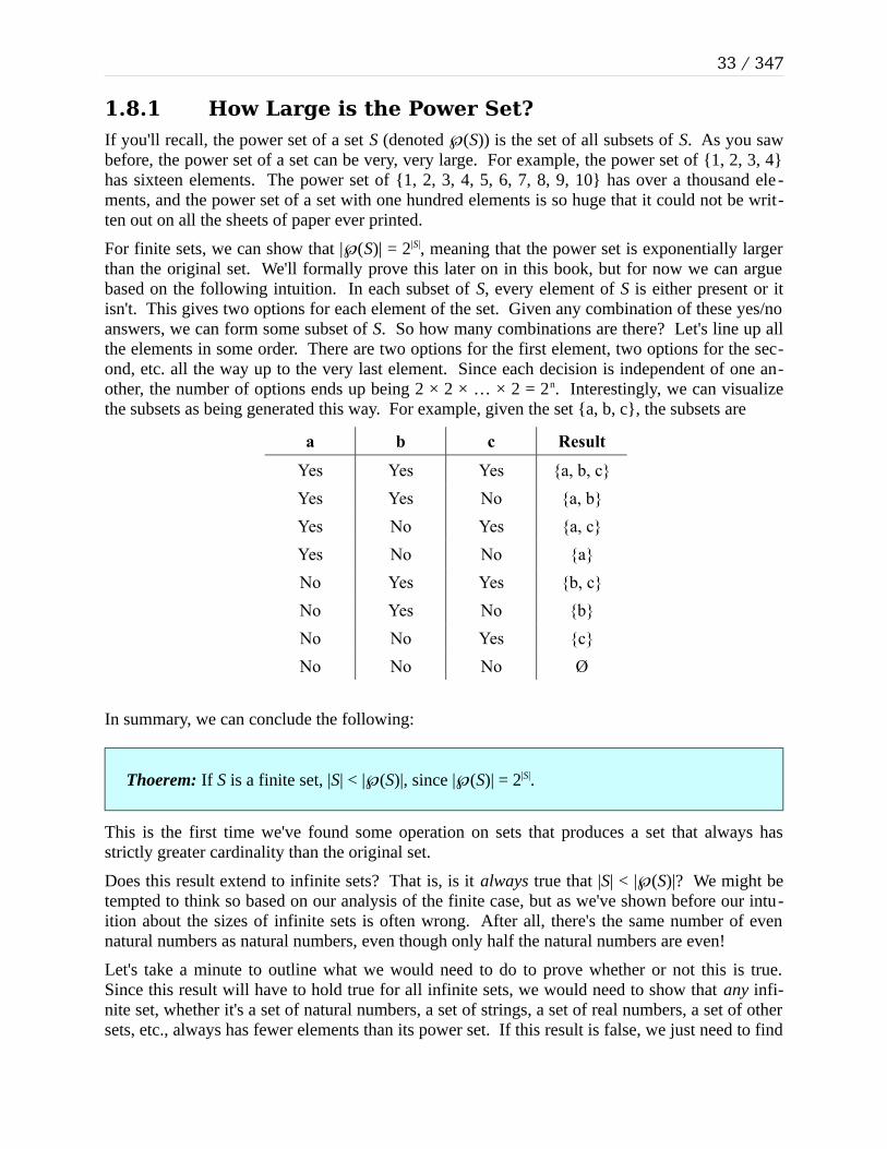
For finite sets, we can show that | (℘ S)| = 2|S|, meaning that the power set is exponentially larger than the original set. We'll formally prove this later on in this book, but for now we can argue based on the following intuition. In each subset of S, every element of S is either present or it isn't. This gives two options for each element of the set. Given any combination of these yes/no answers, we can form some subset of S. So how many combinations are there? Let's line up all the elements in some order. There are two options for the first element, two options for the sec-ond, etc. all the way up to the very last element. Since each decision is independent of one an-other, the number of options ends up being 2 × 2 × … × 2 = 2n. Interestingly, we can visualize the subsets as being generated this way. For example, given the set {a, b, c}, the subsets are

a b c Result

Yes Yes Yes {a, b, c}

Yes Yes No {a, b}

Yes No Yes {a, c}

Yes No No {a}

No Yes Yes {b, c}

No Yes No {b}

No No Yes {c}

No No No Ø

In summary, we can conclude the following:

Thoerem: If S is a finite set, |S| < | (℘ S)|, since | (℘ S)| = 2|S|.

This is the first time we've found some operation on sets that produces a set that always has strictly greater cardinality than the original set.

Does this result extend to infinite sets? That is, is it always true that |S| < | (℘ S)|? We might be tempted to think so based on our analysis of the finite case, but as we've shown before our intu-ition about the sizes of infinite sets is often wrong. After all, there's the same number of even natural numbers as natural numbers, even though only half the natural numbers are even!

Let's take a minute to outline what we would need to do to prove whether or not this is true. Since this result will have to hold true for all infinite sets, we would need to show that any infi-nite set, whether it's a set of natural numbers, a set of strings, a set of real numbers, a set of other sets, etc., always has fewer elements than its power set. If this result is false, we just need to find

Chapter 1: Sets and Cantor's Theorem

a single counterexample. If there is any set S with |S| ≥ | (℘ S)|, then we can go home and say that the theorem is false. (Of course, being good mathematicians, we'd then probably go ask for which sets the theorem is true!) Amazingly, it turns out that |S| < | (℘ S)|, and the proof is a truly marvelous idea called Cantor's diagonal argument.

1.8.2 Cantor's Diagonal ArgumentCantor's diagonal argument is based on a beautiful and simple idea. We will prove that |S| < | (℘ S)| by showing that no matter what way you try pairing up the elements of S and (℘ S), there is always some element of (℘ S) (that is, a subset of S) that wasn't paired up with anything. To see how the argument works, we'll see an example as applied to a simple finite set. We al-ready know that the power set of this set must be larger than the set itself, but by seeing the diag-onal argument in action in a concrete case it will make clearer just how powerful the argument is.

Let's take the simple set {a, b, c}, whose power set is { Ø, {a}, {b}, {c}, {a, b}, {a, c}, {b, c}, {a, b, c} }. Now, remember that two sets have the same cardinality if there's a way of pairing up all of the elements of the two sets. Since we know for a fact that the two sets don't have the same cardinality, there's no possible way that we can do this. However, we know this only because we happen to already know the sizes of the two sets. In other words, we know that there must be at least one subset of {a, b, c} that isn't paired up, but without looking at all of the elements in the pairing we can't necessarily find it. The diagonal argument gives an ingenious way of taking any alleged pairing of the elements of S and its power set and producing some set that is not paired up. To see how it works, let's begin by considering some actual pairing of the elements of {a, b, c} and its power set; for example, this one:

a ↔ {a, b}

b ↔ Ø

c ↔ {a, c}

Now, since each subset corresponds to a set of yes/no decisions about whether each element of {a, b, c} is included in the subset, we can construct a two-dimensional grid like this one below:

a? b? c?

a paired with Y Y N

b paired with N N N

c paired with Y N Y

Here, each row represents the set that each element of {a, b, c} is paired with. The first row shows that a is paired with the set that contains a, contains b, but doesn't contain c, namely {a, b} (indeed, a is paired with this set). Similarly, b is paired with the set that doesn't contain a, b, or c, which is the empty set. Finally, c is paired with the set containing a and c but not b: {a, c}.

Notice that this grid has just as many rows as it has columns. This is no coincidence. Since we are pairing the elements of the set {a, b, c} with subsets of {a, b, c}, we will have one row for each of the elements of {a, b, c} (representing the pairing between each element and some sub-

35 / 347

set) and one column for each of the elements of {a, b, c} (representing whether or not that ele-ment appears in the paired set). As a result, we can take a look at the main diagonal of this ma-trix, which runs from the upper-left corner to the lower-right corner. This is highlighted below:

a? b? c?

a paired with Y Y N

b pared with N N N

c paired with Y N Y

Notice that this diagonal has three elements, since there are three rows and three columns (repre-senting the three elements of the set). This means that the diagonal, as a series of Y's and N's, can potentially be interpreted as a subset of {a, b, c}! In this case, since it includes a, excludes b, and includes c, then it would correspond to the set {a, c}. This set might already be paired with some element (in this case, it is – it's paired with c), though it doesn't have to be.

Cantor's brilliant trick is the following: suppose that we complement the diagonal of this matrix. That is, we'll take the diagonal and flip all the Y's to N's and N's to Y's. In the above case, this gives the following:

a? b? c?

a paired with Y Y N

b paired with N N N

c paired with Y N Y

Complemented Diagonal N Y N

This complemented diagonal represents some subset of {a, b, c}. In this case, it's the set {b}. Now, does this set appear anywhere in the table? It turns out that we can guarantee that this set isn't paired with anything. Here's why. Let's look at the first row of the table. This row can't be the set {b}, because this row and the complemented diagonal disagree at their first position (the first row has a Y, the complemented diagonal has an N). So let's look at the second row. This row can't be the set {b} because it disagrees in the second position – there's an N in the second spot of the second row and a Y in the second spot of the complemented diagonal. Similarly, the third row disagrees in the third position, because there's a Y in the third spot of the third row and an N in the third spot of the complemented diagonal.

The deviousness of complementing the diagonal lies in the fact that we have specifically crafted a set that can't be paired with anything. The reason for this is as follows:

1. Consider any row n in the table.

2. That row can't be equal to the complemented diagonal, because it disagrees in the nth po-sition.

3. Consequently, no row in the table is equal to the complemented diagonal.

Chapter 1: Sets and Cantor's Theorem

Since the rows of the table represent all of the subsets paired with the elements of {a, b, c}, the fact that none of the rows are equal to the complemented diagonal guarantees us that the set rep-resented by the complemented diagonal cannot possibly be paired up with any of the elements of the set! In other words, this diagonal argument gives us a way to take any pairing of the ele-ments of {a, b, c} and its subsets and producing at least one subset that wasn't paired up. To see this argument in action again, here's another pairing:

a ↔ {a}

b ↔ {b}

c ↔ {a, b}

This gives the following table and complemented diagonal:

a? b? c?

a paired with Y N N

b paired with N Y N

c paired with Y Y N

Complemented Diagonal N N Y

The complemented diagonal here is {c}, which is missing from the table.

If we didn't already know that the power set of {a, b, c} was bigger than the set {a, b, c}, this di -agonal argument would have just proven it – it gives a way of taking any possible pairing of the elements of {a, b, c} with its subsets and shows that after pairing up all the elements of {a, b, c}, there is always some element left uncovered. This same technique can be applied to other sets as well. For example, suppose we have the set {a, b, c, d, e, f}, and this pairing:

a ↔ {b, c, d}

b ↔ {e, f}

c ↔ {a, b, c, d, e, f}

d ↔ Ø

e ↔ {a, f}

f ↔ {b, c, d, e}

We can then build the following table, which has its diagonal and complemented diagonal shown:

37 / 347

a? b? c? d? e? f?

a paired with N Y Y Y N N

b paired with N N N N Y Y

c paired with Y Y Y Y Y Y

d paired with N N N N N N

e paired with Y N N N N Y

f paired with N Y Y Y Y N

Complemented Diagonal Y Y N Y Y Y

From this, we get that the complemented diagonal is the set {a, b, d, e, f}, which indeed is not in the list of sets described in the pairing.

1.8.3 Formalizing the Diagonal ArgumentWe have just described the intuition behind Cantor's diagonal argument – we can show that in any pairing between a set S and the set (℘ S), there must be some element of (℘ S) that isn't cov-ered by the pairing. However, so far our proof requires us to construct a table representing the pairing whose size is determined by the number of elements in S. Given this, will this argument work when we are dealing with infinite sets? We've seen a lot of strange results that appear when working with the infinite, and so it doesn't seem particularly “safe” to assume that this ap-proach, which works in the finite case, scales up to the infinite case.

It turns out, however, that this argument can indeed be applied to infinite sets! However, to do so will require us to be more precise and formal than our reasoning above, in which we just drew a picture. We need to find a way of nicely describing what set is constructed by the diagonal argu-ment without having to draw out a potentially infinite table. Fortunately, there is a nicely straightforward way to do this. Let's consider the previous example:

a ↔ {b, c, d}

b ↔ {e, f}

c ↔ {a, b, c, d, e, f}

d ↔ Ø

e ↔ {a, f}

f ↔ {b, c, d, e}

Chapter 1: Sets and Cantor's Theorem

a? b? c? d? e? f?

a paired with N Y Y Y N N

b pared with N N N N Y Y

c paired with Y Y Y Y Y Y

d paired with N N N N N N

e paired with Y N N N N Y

f paired with N Y Y Y Y N

Complemented Diagonal Y Y N Y Y Y

Now, let's think about the diagonal of this table. Notice that each diagonal entry represents whether some element x ∈ S is paired with a set that contains itself. If the element x is paired with a set that contains it, the the entry on the diagonal is a Y, and if x is paired with a set that doesn't contain it, then the entry on the diagonal is an N. In the complemented diagonal, this is reversed – the complemented diagonal entry is a Y if x is paired with a set that doesn't contain x, and is an N if x is paired with a set that does contain x. In other words, we can think about the set defined by the complemented diagonal (let's call it D) as follows:

D = { x | there is an N in the diagonal entry for x }

Or, more concretely:

D = { x | x is paired with a set that does not contain x }

Now this is interesting – we now have a definition of the diagonal set D that doesn't require us to even construct the table! The rule for finding D is straightforward: we simply find all the ele-ments of the set S that are paired with subsets of S that don't contain themselves, then gather those up together into a set. Does this really work? Well, if experience is a guide, then yes! Here are a few pairings from before, along with the associated diagonal set:

Pairinga   {a}↔b   {b}↔

c   {a, b}↔

a   {a, b}↔b   Ø↔

c   {a, c}↔

a   {b, c, d}↔b   {e, f}↔

c   {a, b, c, d, e, f}↔d   Ø↔

e   {a, f}↔f   {b, c, d, e}↔

ComplementedDiagonal Set {c} {b} {a, b, d, e, f}

You can (and should!) check that in each case, the complemented diagonal set is indeed the set of elements that aren't paired with a set that contains them. For example, in the first example since a is paired with {a} and b is paired with {b}, neither is included in the complemented diagonal set, while c, which is paired with a set that doesn't contain c, is indeed in the complemented diag-onal set.

39 / 347

1.8.4 Proving Cantor's TheoremGiven this definition of the diagonal set, we can formally prove Cantor's theorem.

Theorem (Cantor's Theorem): For any set S, |S| < | (℘ S)|.

In order to prove Cantor's theorem, let's think about the definition of what it means for one set to have lesser cardinality than another. This would mean that

|S| ≤ | (℘ S)| and |S| ≠ | (℘ S)|

We can prove each part of this independently. Cantor's diagonal argument will handle the second case (which we'll handle in a minute), but first let's show that |S| ≤ | (℘ S)|. How can we show this? To do so, we need to show that we can pair off all of the elements of S with some element in (℘ S). This might seem hard, because we don't actually know what S is; we need to show that for any set S, it's always possible to find such a pairing. This actually ends up being not too diffi-cult. Note that for each element x ∈ S, the set {x} ⊆ S. Therefore, {x} (∈ ℘ S). Consequently, one way of pairing up all the elements of S with elements from (℘ S) would be to associate each element x ∈ S with the element {x} ∈ (℘ S). This ensures that each element of S is paired up with a unique element from (℘ S).

Now, we need to formally prove that |S| ≠ | (℘ S)|, even though we don't actually know what S is (we're trying to prove the claim for any possible choice of S). So what does it mean for|S| ≠ | (℘ S)|? Well, this would mean that there must be no possible way of pairing off all the ele-ments from the two sets with one another. How can we show that this is impossible? Here, we will employ a technique called proof by contradiction. In a proof by contradiction, we try to show that some statement P is true by doing the following:

• Assume, hypothetically, that P was false.

• Show that this assumption, coupled with sound reasoning, leads us to a conclusion that is obviously false.

• Conclude, therefore, that our assumption must have been wrong, so P is true.

As an example of a proof of this style, suppose that you want to convince someone that it is not raining outside (if it's raining when you're reading this, then my apologies – please bear with me!) One way to convince someone that it's not raining is as follows:

1. Suppose, hypothetically, that it were raining.

2. Therefore, I should be soaking wet from my walk a few minutes ago.

3. But I am not soaking wet from my walk a few minutes ago.

4. Since steps (2) and (3) are logically sound, the only possible problem is step (1).

5. Conclude, therefore, that it's not raining outside.

Here, when proving that |S| ≠ | (℘ S)|, we will use a proof by contradiction. Suppose, hypotheti-cally, that |S| = | (℘ S)|. Then there is a way of pairing up all of the elements of S and (℘ S) to-gether – we don't know what it is, but allegedly it exists. This should mean that any element of

(℘ S) that we choose should be paired up with some element of S. Since every element of (℘ S)

Chapter 1: Sets and Cantor's Theorem

is a subset of S (that's how we defined the power set!), this should mean that if we choose any subset of S, it should be paired up with some element from S. But now we can employ Cantor's diagonal argument. If it's really true that any subset of S must be paired up with some element of S, then surely we should be able to find some element paired up with the set

D = {x | x ∈ S and x is paired with a set that does not contain x. }

Well, since D allegedly must be paired with something, let's call that element d. But if you'll re-call from our discussion of the diagonal argument, we should now be able to show that D actu-ally isn't in this table, meaning that there really isn't an element d that it could be paired with. But how do we show this? Here, we'll simply ask the following question: is d contained in D? There are two possible options: either d ∈ D or d ∉ D. Let's consider these two cases individu-ally.

First, suppose that d ∈ D. Recall that the definition of D says that this means that d would have to be paired with a set that doesn't contain d. Since d is paired with D, this would have to mean that d ∉ D, but this is clearly impossible, because we know that in this case d ∈ D. Since if d ∈ D we conclude that d ∉ D, we know that it must not be possible for d ∈ D to be true.

So this means that d ∉ D. Well, let's see what that means. Since d ∉ D, then by looking at the definition of the set D, we can see that this means that the set that d is paired with must contain d. Since d is paired with the set D, this would mean that d ∈ D. But this isn't true!

We have just reached a logical contradiction. If d ∈ D, then we know that d ∉ D, and similarly if d ∉ D, then d ∈ D. In other words, D contains d if and only if D does not contain d. We have reached a logical impossibility.

All of the reasoning we've had up to this point is sound, so we are forced to admit that the only possibility remaining is that our assumption that |S| = | (℘ S)| is incorrect. Consequently, we have proven that |S| ≠ | (℘ S)|. Since earlier we proved |S| ≤ | (℘ S)|, this collectively proves Cantor's theorem.

1.9 Why Cantor's Theorem MattersWe have just proven Cantor's theorem, that the number of subsets of a set S is strictly greater than the number of elements of that set S. But why does this matter? It turns out that this is ac-tually a hugely important result with a terrifying corollary. To begin with, note that Cantor's the-orem says that there are more subsets of a set than elements of that set, even if the initial set is in-finite. This suggests that there is no one concept of “infinity,” and that there are, in fact, different infinitely large quantities, each one infinitely larger than the previous! In fact this means that

• There are more sets of natural numbers than natural numbers (|ℕ| < | (℘ ℕ)|)

• More sets of sets of natural numbers than sets of natural numbers (| (℘ ℕ)| < | ( (℘ ℘ ℕ))|),

• etc.

The fact that there are different infinitely large numbers has enormous significance to the limits of computing. For example, there are infinitely many problems to solve, and there are infinitely many programs to solve them. But this doesn't mean that there are the same number of problems

41 / 347

and solutions! In fact, it might be possible that there are more problems that we might want to solve than there are programs to solve them, even though both are infinite! In fact, this is the case. Let's see why.

1.10 The Limits of ComputationLet's begin with a pair of definitions:

An alphabet is a set of symbols.

For example, we could talk about the English alphabet as the set A = { A, B, C, D, …, Y, Z, a, b, …, z }. The binary alphabet is the alphabet {0, 1}, and the unary alphabet is the alphabet { 1 }. Given an alphabet, what words can we make from that alphabet? Typically, we will use the term “string” instead of “word:”

A string is a finite sequence of symbols drawn from some alphabet.

For example, hello is a string drawn from the English alphabet, while 01100001 is a string drawn from the binary alphabet.

Every computer program can be expressed as a string drawn from the appropriate alphabet. The program's source code is a sequence of characters (probably Unicode characters) that are trans-lated into a program using a compiler. In most programming languages, not all strings are legal programs, but many are. As a result, we can say that the number of programs is at most the num-ber of strings, since we can pair up the programs and strings without exhausting all strings (just pair each program with its source code).

Now, let's think about how many problems there are out there that we might want to solve. This really depends on our notion of what a “problem” is, but we don't actually need to have a formal definition of “problem” quite yet. Let's just focus on one type of problem: deciding whether a string has some property. For example, some strings have even length, some are palindromes, some are legal Java programs, some are mathematical proofs, etc. We can think of a “property” of a string as just a set of strings that happen to share that property. For example, we could say that the property of being a palindrome (reading the same forwards and backwards) could be rep-resented by the set

{ a, b, c, …, z, aa, bb, …, zz, aba, aca, ada, … }

While the property of having exactly four letters would be

{ aaaa, aaab, aaac, …, zzzz }

For each of these properties, we might think about writing a program that could determine whether a string has that given property. For example, with a few minutes' effort you could probably sit down and write a program that will check whether a string is a palindrome or con-tains just four characters, and with more effort could check if a string encoded a legal computer program, etc. In other words, each property of strings (that is, a set of strings) defines a unique

Chapter 1: Sets and Cantor's Theorem

problem – determine whether a given string has that property or not. As a result, the number of sets of strings is no bigger than the total number of problems we might want to solve, since there's at least one problem to solve per set of strings.

This leads to the following line of reasoning:

The number of programs is no bigger than the number of strings.

The number of strings is strictly less than the number of sets of strings (from Cantor's theorem).

The number of properties of strings is bigger than the number of strings.

Since each property of strings gives rise to a problem to solve:

The number of problems is at least the number of properties of strings.

Combining this all together gives the following:

The number of programs is strictly less than the number of problems.

In other words:

There are more problems than there are programs to solve them.

We have just proven, without even looking at how computers work or how clever programmers are, that there are problems that cannot possibly be solved by a computer. There are simply too many problems to go around, so even if we wrote all of the infinitely many possible programs, we would not have written a program to solve every problem.

1.10.1 What Does This Mean?At this point, we could throw up our hands and despair. We have just shown the existence of un-solvable problems, problems that can be formulated but not possibly solved.

Unfortunately, it gets worse. Using more advanced set theory, we can show that the infinity of problems so vastly dwarfs the infinity of solutions that if you choose a totally random problem to solve, the chance that you can is 0. Moreover, since there are more problems to solve than possi-ble strings, some of the problems we can't solve may be so complex that there is no way to de-scribe them; after all, a description is a way of pairing a string with a problem!

But there's no way we can give up now. We have shown that there is an infinite abyss of unsolv-able problems, but everywhere we look we can see examples of places where computers have solved problems.

Rather than viewing this result as a sign of defeat, treat it as a call to arms. Yes, there are infin-itely many problems that we can't solve, but there are infinitely many problems that we can solve as well. What are they? What do they look like? Of the problems we can solve in theory, what can be solved in practice as well? How powerful of a computer would you need to solve them? These are questions of huge practical and theoretical importance, and its these questions that we will focus on in the rest of this book. In doing so, you'll sharpen your mathematical acu-men and will learn how to reason about problems abstractly. You'll learn new ways of thinking about computation and how it can impact your practical programming skills. And you'll see some of the most interesting and fascinating results in all of computer science.

Let's get started!

43 / 347

1.11 Chapter Summary• A set is an unordered collection of distinct elements.

• Sets can be described by listing their elements in some order.

• Sets can also be described using set-builder notation.

• Set can be combined via union, intersection, difference, or symmetric difference.

• Two sets are equal precisely when they have the same elements.

• One set is a subset of another if every element of that set is in the other set.

• The power set of a set is the set of its subsets.

• A statement is vacuously true if its assertion doesn't apply to anything.

• The cardinality of a set is a measure of how many elements are in that set.

• Two sets have the same cardinality if all elements of both sets can be paired up with one another.

• Cantor's diagonal argument can be used to prove Cantor's theorem, that the cardinality of a set is always strictly less than the cardinality of its power set.

Chapter 2 Mathematical ProofLast chapter we concluded with Cantor's theorem, the fact that the cardinality of the power set of a set S is always greater than the cardinality of the set S itself. Although we worked through a strong argument that this should be true, did we really “prove” it? What does it mean to prove something, at least in a mathematical sense?

Proofs are at the core of the mathematical foundations of computing. Without proofs we couldn't be certain that any of our results were correct, and our definitions would be little better than an intuition to guide us. Accordingly, before we attempt to explore the limits of computation, we first need to build up the machinery necessary to reason about and firmly establish mathematical results.

Proofs are in many ways like programs – they have their own vocabulary, terminology, and struc-ture, and you will need to train yourself to think differently in order to understand and synthesize them. In this chapter and the ones that follow, we will explore proofs and proof techniques, along with several other concepts that will serve as a “proving ground” for testing out these proof ideas.

One quick note before we continue – because this chapter focuses on how to structure mathemat-ical proofs, some of the results that we'll be proving early on will be pretty trivial. I promise you that the material will get a lot more interesting toward the end of the chapter, and once we make it into Chapter Three the results we will be proving will be much more involved and a lot more interesting. Please don't get the impression that math is painfully boring and pedantic! It's a re-ally fascinating subject, but we need to build up a few techniques before we can jump into the real meat of the material.

2.1 What is a Proof?In order to write a proof, we need to start off by coming up with some sort of definition of the word “proof.” Informally, a mathematical proof is a series of logical steps starting with one set of assumptions that ends up concluding that some statement must be true. For example, if we wanted to prove the statement

If x + y = 16, then either x ≥ 8 or y ≥ 8

Then we would begin by assuming that x + y = 16, then apply sound logical reasoning until we had arrived at the conclusion that x ≥ 8 or y ≥ 8. Similarly, if we wanted to prove that

For any set S, |S| < | (℘ S)|

(as we started doing last chapter), we would take as our starting point all of the definitions from set theory – what the power set is, what it means for one set to have smaller cardinality than an-other, etc. - and would proceed through logical steps to conclude that |S| < | (℘ S)|.

Writing a proof is in many ways like writing a computer program. You begin with some base set of things that you know are true (for example, how primitive data types work, how to define classes, etc.), then proceed to use those primitive operations to build up something more compli-cated. Also like a program, proofs have their own vocabulary, language, structure, and expecta-

Chapter 2: Mathematical Proof

tions. Unfortunately, unlike programs, there is no “compiler” for proofs that can take in a proof and verify that it's a legal mathematical proof.* Consequently, learning how to write proofs takes time and effort.

In this chapter, we will introduce different types of proofs by analyzing real proofs and seeing exactly how they work. We'll also see what doesn't work and the sort of logical traps you can easily fall into when writing proofs.

2.1.1 What Can We Assume?One of the most difficult aspects of writing a proof is determining what you can assume going into the proof. In journals, proofs often assume that the reader is familiar with important results, and often cite them without reviewing why they're true. For our purposes, though, we will delib-erately play dumb and start with a very weak set of assumptions. We will prove pretty much ev-erything we need, even if it seems completely obvious, in order to see how to formalize intuitive concepts with a level of mathematical rigor.

In this book, we will assume that whoever is reading one of our proofs knows

1. All definitions introduced so far,

2. All theorems introduced so far, and

3. Basic algebra.

We will not assume anything more than this. For example, we're fine assuming that if x < y and y < z, then x < z, but we will not assume that for any set S, S ∩ Ø = Ø even though this seems “obvious.” As we build up our mathematical repertoire, the set of assumptions we can make will grow, and it will become easier and easier to prove more elaborate results. This is similar to writing libraries in computer programs – although it's difficult and a bit tedious to implement standard data structures like ArrayList and HashMap, once you've put in the work to do so it becomes possible to build up off of them and start writing much more intricate and complex pro-grams.

2.2 Direct ProofsJust as it's often easiest to learn how to program by jumping into the middle of a “Hello, World!” program and seeing how it works, it's useful to jump right into some fully worked-out mathemat-ical proofs to see how to structure general proofs.

To begin our descent into proofs, we'll introduce two simple definitions, then see how to prove results about those definitions.

An integer x is called even if there is some integer k such that x = 2k.

An integer x is called odd if there is some integer k such that x = 2k + 1.

* Technically speaking such programs exist, but they require the proof to be specified in a very rigid format that is almost never used in formal mathematical proofs.

47 / 347

For example, 4 is even since 4 = 2 × 2. 8 is even as well, since 8 = 4 × 2. 9 is odd, because 9 = 4 × 2 + 1. We consider 0 to be an even number, since 0 = 0 × 2.

Given this, let's prove the following result:

Theorem: If x is even, then x2 is even.

Proof: Let x be any even integer. Since x is even, there is some integer k such that x = 2k. This means that x2 = (2k)2 = 4k2 = 2(2k2). Since 2k2 is an integer, this means that there is some integer m (namely, 2k2) such that x2 = 2m. Thus x2 is even. ■

Let's look at how this proof works. The proof proceeds in several clean logical steps, each of which we can analyze independently.

First, note how the proof starts: “Let x be any even integer.” The goal of this proof is to show that if x is even, then x2 is even as well. This proof should work no matter what choice of x we make – whether it's 0, 2, 4, 6, 8, etc. In order for our proof to work in this general setting, the proof will proceed by using x as a placeholder for whatever even number we're interested in. If we wanted to convince ourselves that some particular even number has a square that's also even, we could just plug that even number into the proof wherever we were using x. For example, if we want to prove that 122 is even, the proof would go like this:

Proof: Since 12 is even, there is some integer k such that 12 = 2k. (This integer k is the in-teger 6). This means that 122 = (2 × 6)2 = 4 × 62 = 2(2 × 62) = 2 × 72. Since 72 is an inte-ger, this means that there is some integer m (namely, 72) such that 122 = 2m. Thus 122 is even. ■

All that we've done here is substitute in the number 12 for our choice of x. We could substitute in any other even number if we'd like and the proof would still hold. In fact, that's why the proof works – we've shown that no matter what choice of an even number you make for x, you can al-ways prove that x2 is even as well.

Let's continue dissecting this proof. After we've decided to let x be a placeholder for whatever even number we'd like, we then say

Since x is even, there is some integer k such that x = 2k

What does this statement mean? Well, we know that x is an even number, which means that it must be twice some other number. We can't really say what that number is, since we don't know what our choice of x is. However, we can say that there is some number such that x is twice that number. In order to manipulate that number in this proof, we'll give this number a name (in this proof, we call it k). Interestingly, note that nowhere in this sentence do we actually say how to figure out what this value of k is; we just say that it has to exist and move forward. From a pro-gramming perspective, this may seem strange – it seems like we'd have to show how to find this

Chapter 2: Mathematical Proof

number k in order to assert that it exists! But it turns out that it's perfectly fine to just say that it exists and leave it at that. Our definition of an even number is an integer that is equal to twice some other number, so we know for a fact that because x is even, this number k must exist.

At this point, we know that x = 2k, and our goal is to show that x2 is even. Let's think about how to do this. To show that x2 is even, we will need to find some integer m such that x2 = 2m. Right now, all that we know that is that x is even and, as a result, that x = 2k for some choice of k. Since we don't have much else to go on right now, let's try seeing if we can describe x2 in terms of x and k. Perhaps doing this will lead us to finding some choice of m that we can make such that x2 = 2m. This leads to the next part of the proof:

This means that x2 = (2k)2 = 4k2 = 2(2k2). Since 2k2 is an integer, this means that there is some integer m (namely, 2k2) such that x2 = 2m

The first of these two sentences is a simple algebraic manipulation. We know that x = 2k, so x2 = (2k)2. If we simplify this, we get x2 = 4k2, which is in turn equal to 2(2k2). This last step – factor-ing out the two from the expression – then makes it clearer that x2 is twice some other integer (specifically, the integer 2k2). We can then conclude that there is some natural number m such that x2 = 2m, since we've found specifically what that value was. Because we've done this, we can conclude the proof by writing:

Thus x2 is even. ■

This holds because the definition of an even number is one that can be written as 2m for some in-teger m. Notice that we've marked the end of the proof with the special symbol ■, which serves as a marker that we're done. Sometimes you see proofs ended with other statements like “This completes the proof” or “QED” (from the Latin “quod erat demonstrandum,” which translates roughly to “which is what we wanted to show”). Feel free to end your own proofs with one of these three endings.

Let's take a look at an example of another proof:

Theorem: If m is even and n is odd, then mn is even.

Proof: Let m be any even number and n be any odd number. Then m = 2r for some integer r, and n = 2s + 1 for some integer s. This means that mn = (2r)(2s + 1) = 2(r(2s + 1)). This means that mn = 2k for some integer k (namely, r(2s + 1)), so mn is even. ■

The structure of this proof is similar to the previous proof. We want to show that the claim holds for any choice of even m and odd n, so we begin by letting m and n be any even and odd number, respectively. From there, we use the definition of even and odd numbers to write m = 2r and n as 2s + 1 for some integers r and s. As with the previous proof, we don't actually know what these

49 / 347

numbers are, but they're guaranteed to exist. After doing some simple arithmetic, we end up see-ing that mn = 2(r(2s + 1)), and since r(2s + 1) is an integer, we can conclude that mn is twice some integer, and so it must be even.

The above proofs are both instances of direct proofs, in which the proposition to be proven is di-rectly shown to be true by beginning with the assumptions and ending at the conclusions.

2.2.1 Proof by CasesLet's introduce one new definition, which you may be familiar with from your programming background:

The parity of an integer is whether it is odd or even. Two numbers have the same parity if they are both odd or both even.

For example, 1 and 5 have the same parity, because both of the numbers are odd, and 4 and 14 have the same parity because both 4 and 14 are even. However, 1 and 2 have opposite parity, be-cause 1 is odd and 2 is even.

The following result involves the parity of integers:

Theorem: If m and n have the same parity, then m + n is even.

Before we try to prove this, let's check that it's actually correct by testing it on a few simple ex-amples. We can see that 2 + 6 = 8 is even, and 1 + 5 = 6 is even as well. But how would we prove that this is true in the general case? In a sense, we need to prove two separate claims, since if m and n have the same parity, then either both m and n are even or both m and n are odd. The definitions of odd numbers and even numbers aren't the same, and so we have to consider the two options separately. We can do this cleanly in a proof as follows:

Proof: Let m and n be any two integers with the same parity. Then there are two cases to consider:

Case 1: m and n are even. Then m = 2r for some integer r and n = 2s for some integer s. Therefore, m + n = 2r + 2s = 2(r + s). Thus m + n = 2k for some integer k (namely, r + s), so m + n is even.

Case 2: m and n are odd. Then m = 2r + 1 for some integer r and n = 2s + 1 for some inte-ger s. Therefore, m + n = 2r + 1 + 2s + 1 = 2r + 2s + 2 = 2(r + s + 1). Thus m + n = 2k for some integer k (namely, r + s + 1), so m + n is even. ■

Note how this proof is structured as two cases – first, when m and n are even, and second, when m and n are odd. This style of proof is sometimes called a proof by cases or a proof by exhaus-tion (because we've exhausted all possibilities and found that the claim is true). Each of the

Chapter 2: Mathematical Proof

branches of the proof reads just like a normal proof, but is individually insufficient to prove the general result. Only when we show that in both of the possible cases the result holds can we conclude that the claim is true in general.

When writing a proof by exhaustion, it's critically important to remember to check that you have covered all possible cases! If you have a proof where four options are possible and you only prove three cases, your proof is likely to be incorrect.

Let's see another example of a proof by cases:

Theorem: If n is even and m is an integer, then n + m has the same parity as m.

Before proving this, it's always good to check that it works for a few test cases. If we let n = 4, then we can see that

• 4 + 3 = 7, and 7 has the same parity as 3.

• 4 + 6 = 10, and 10 has the same parity as 6.

Let's see a proof of this result:

Proof: Consider any even integer n. Now, consider any integer m and the sumn + m. We consider two possibilities for m:

Case 1: m is even. Then m and n have the same parity, so by our previous result (if m and n have the same parity, then m + n is even) we know that m + n is even. Therefore m and m + n have the same parity.

Case 2: m is odd. Since n is even, n = 2r for some integer r, and since m is odd,m = 2s + 1 for some integer s. Then n + m = 2r + 2s + 1 = 2(r + s) + 1. This means thatn + m = 2k + 1 for some k (namely, r + s), so n + m is odd. Therefore m and m + n have the same parity. ■

This proof is interesting for two reasons. First, notice that in proving that Case 1 is true, we used the result that we have proven previously: if n and m have the same parity, then n + m is even. This means that we didn't have to try writing n = 2r and m = 2s, and we ended up saving a lot of space in our proof. Whenever you're writing a proof, feel free to cite any result that you have previously proven. In CS103, it's perfectly fine to cite proofs from lecture, this book, or the problem sessions, as long as you make it clear what result you're using.

Second, notice that in this proof the cases resulted from the parity of just one of the variables (m). We knew that the parity of n must be even, and the only thing that was unclear was whether m was odd or even.

51 / 347

2.2.1.1 A Quick Aside: Choosing Letters

If you'll notice, the proofs that we've done so far use lots of letters to stand for numbers: m, n, k, r, s, etc. In general, when writing a proof, you should feel free to choose whatever letters you think will make the proof flow most cleanly. However, you should make an effort to pick a con-sistent naming convention, much in the same way that you should adopt a naming convention when writing computer programs.

In this set of course notes, I will typically use single capital letters (S, T, U) to represent sets. I tend to use the letters m, n, and k to represent natural numbers and x, y, z to represent integers. If I run out of letters, I might borrow others from other parts of the alphabet (for example, r, s, and t for natural numbers if we exhaust our normal supply.

When working with values in a sequence (more on that later), I'll tend to use subscripted symbols like x1, x2, …, xi. In those cases, the letters i, j, and k will typically refer to variable indices, and n will represent quantities like the total number of elements in the sequence.

2.2.2 Proofs about SetsIn the last chapter, we explored sets and some of the operations on them. You have already seen one theorem about sets (specifically, Cantor's theorem). But what else can we prove about sets? And how do we prove them?

Let's begin with a very simple proof about sets:

Theorem: For any sets A and B, A ∩ B ⊆ A.

This theorem intuitively makes sense. We can think of A ∩ B as the set of things that A and B have in common. In other words, we're filtering down the elements of A by just considering those elements that also happen to be in B. As a result, we should end up with a set that's a sub-set of the set A. So how do we prove this? As you will see, the proof works similarly to our proof about odd and even numbers: it calls back to the definitions of intersection and subset, then proceeds from there.

Proof: Consider any sets A and B. We want to show that A ∩ B ⊆ A. By the definition of subset, this means that we need to show that for any x ∈ A ∩ B, x ∈ A. So consider any x ∈ A ∩ B. By the definition of intersection, x ∈ A ∩ B means that x ∈ A and x ∈ B. Therefore, if x ∈ A ∩ B, x ∈ A. Since our choice of x was arbitrary, A ∩ B ⊆ A. ■

Let's examine the structure of the proof. We initially wanted to prove that A ∩ B ⊆ A. To do this, we said something to the effect of “okay, I need to prove that A ∩ B ⊆ A. What does this mean?” By using the definition of subset, we were able to determine that we needed to prove that for any choice of x ∈ A ∩ B, it's true that x ∈ A. Again we ask – so what does it mean for x ∈ A ∩ B? Again we call back to the definition: x ∈ A ∩ B means that x ∈ A and x ∈ B. But at this point we're done – we needed to show that any x ∈ A ∩ B also satisfies x ∈ A, but the very definition of A ∩ B guarantees this to us!

Chapter 2: Mathematical Proof

This proof illustrates a crucial step in many proofs – if you are unsure about how to proceed, try referring to the definitions of the terms involved. Often this simplification will help you make progress toward the ultimate proof by rewriting complex logic in terms of something similar.

Let's do another simple proof:

Theorem: For any sets A and B, A ⊆ A ∪ B.

This result says that if we take any collection of things (the set A) and combine it together with any other set of things (forming the set A ∪ B), then the original set is a subset of the resulting set. This seems obvious – after all, if we mix in one set of things with another, that initial set is still present! Of course, it's good to formally establish this, which we do here:

Proof: Consider any sets A and B. We want to show that A ⊆ A ∪ B. To do this, we show that for any x ∈ A, that x ∈ A ∪ B as well. Note that by definition, x ∈ A ∪ B iff x ∈ A or x ∈ B.

Consider any x ∈ A. It is therefore true that x ∈ A or x ∈ B, since we know x ∈ A. Conse-quently, x ∈ A ∪ B. Since our choice of x was arbitrary, this shows that any x ∈ A also satisfies x ∈ A ∪ B. Consequently, A ⊆ A ∪ B, as required. ■

Again, notice the calling back to the definitions. To prove A ⊆ A ∪ B, we argue that every x ∈ A also satisfies x ∈ A ∪ B. What does it mean for x ∈ A ∪ B? Well, the definition of A ∪ B is the set of all x such that either x ∈ A or x ∈ B. From there we can see that we're done – if x ∈ A, then it's also true that x ∈ A or x ∈ B, so it's true that x ∈ A ∪ B.

Let's do another proof, this time proving a slightly more complex result:

Theorem: For any sets A, B, and C, we have C – (A ∩ B) (⊆ C – A) (∪ C – B)

As an example, let's take A = {1, 2, 3}, B = {3, 4, 5}, and C = {1, 2, 3, 4, 5}. Then we have that

C – (A ∩ B) = {1, 2, 3, 4, 5} – {3} = {1, 2, 4, 5}.

We also have that

(C – A) (∪ C – B) = {4, 5} {1, 2} = {1, 2, 4, 5}.∪

Thus in this single case, C – (A ∩ B) (⊆ C – A) (∪ C – B), since the two sets are equal.

This theorem worked out in the above case, but it's not at all clear exactly why this would be true. How, then, could we prove this?

Whenever you need to write a proof, always be sure that you understand why what you're prov-ing is true before you try to prove it! Otherwise, you're bound to get stuck. So before we start to work through the actual proof, let's try to build up an intuition for why this result is true. To do so, let's turn to Venn diagrams, which are surprisingly useful when proving results like these.

53 / 347

Let's start with this Venn diagram for three sets:*

A B

C

If we highlight the set A ∩ B, we get this region of the diagram:

A B

C

Given this, we can see that C – (A ∩ B) corresponds to this region:

A B

C

Now, let's take a look at (C – A) (∪ C – B). If we highlight C – A and C – B separately, we get these regions:

* I'm using diamonds instead of circles here because my drawing program (LibreOffice) makes it tricky to fill in circular regions.  If you have any suggestions on how to draw better Venn diagrams, please let me know!

Chapter 2: Mathematical Proof

A B

C

A B

C

Consequently, their union (C – A) (∪ C – B) is this region here:

A B

C

Now it's a bit clearer why this result should be true – the two sets are actually equal to one an -other! Moreover, it's easier to see why. To build up the sets C – (A ∩ B), we can construct the sets C – A and C – B, then combine them together.

That said, the above picture isn't really a mathematical proof in the conventional sense. We still need to write out the proof longhand. To do this, we'll try to translate the above pictorial intu -ition into words. Specifically, we can work as follows. If we take any element of C – (A ∩ B), then (as you can see above) it belongs to at least one of C – A or C – B. We can therefore write a proof by cases and show that regardless of which of these two sets our element belongs to, we know that the element must belong to (C – A) (∪ C – B).

This is formalized below:

Proof: Consider any sets A, B, and C. We will show C – (A ∩ B) (⊆ C – A) (∪ C – B). By definition, this is true if for any x ∈ C – (A ∩ B), we also have x ∈ (C – A) (∪ C – B). So consider any x ∈ C – (A ∩ B). By the definition of set difference, this means that x ∈ C and x ∉ A ∩ B. Since x ∉ A ∩ B, we know that it is not the case that both x ∈ A and x ∈ B. Consequently, it must be true that either x ∉ A or x ∉ B. We consider these two cases individually:

Case 1: x ∉ A. Since we know that x ∈ C and x ∉ A, we know that x ∈ C – A. By our ear-lier result, we therefore have that x (∈ C – A) (∪ C – B).

55 / 347

Case 2: x ∉ B. Since we know that x ∈ C and x ∉ B, we know that x ∈ C – B. By our ear-lier result, we therefore have that x (∈ C – A) (∪ C – B).

In either case we have that x (∈ C – A) (∪ C – B). Since our choice of x was arbitrary, we have that C – (A ∩ B) (⊆ C – A) (∪ C – B) as required. ■

Notice that in the course of this proof, we ended up referring back to the proof we did above in which we claimed that for any sets A and B, A ⊆ A ∪ B. Using this theorem, we were able to conclude that if x ∈ C – A, then x (∈ C – A) (∪ C – B). This is extremely common in mathemat-ics. We begin with a few simple terms and definitions, then build up progressively more elabo-rate results from simpler ones. Most major results do not work from first principles, but instead build off of earlier work by combining well-known results and clever insights.

2.2.3 LemmasLet's think about the simple result that A ⊆ A ∪ B. In itself, this isn't very surprising. The proof is simple and straightforward, and in the end we don't end up with anything particular complex. However, as you saw above, this simple result can be used as a building block for proving more elaborate results.

A result that is primarily used as a small piece in a larger proof is sometimes called a lemma. Lemmas are distinguished from theorems primarily by how they're used. Some lemmas, such as the pumping lemma (which you'll learn more about later) are actually quite impressive results on their own, but are mostly used a step in more complex proofs. Other lemmas, like the one you just saw, are simple but necessary as a starting point for future work.

When proving results about sets, lemmas like A ⊆ A ∪ B are often useful in simplifying more complex proofs. In fact, many seemingly obvious results about sets are best proven as lemmas so that we can use them later on.

The first lemma that we'll actually treat as such is the following result, which helps us prove that two sets are equal to one another:

Lemma: For any sets A and B, A = B if and only if A ⊆ B and B ⊆ A.

Note the use of the phrase if and only if in this lemma. The phrase “P if and only if Q” means that whenever P is true, Q is true, and whenever Q is true, P is true. In other words, “P if and only if Q” means that P and Q have the same truth value – either both P and Q are true, or both P and Q are false. The statement “if and only if” is a very strong assertion – it says that any time we'd like to speak about whether P is true or false, we can instead speak of whether Q is true or false.

As long as we're on the subject, you sometimes see the word iff used to mean “if and only if.” This is a term that we'll use throughout this text, as it's widely used in the mathematical world. Consequently, we might rewrite the above lemma as

Chapter 2: Mathematical Proof

Lemma: For any sets A and B, A = B iff A ⊆ B and B ⊆ A.

Note that “iff” is read aloud as “if and only if.” That way, we don't need to try to differentiate between “if” and “iff” by listening to how long the speaker draws out the final “f.” This means that the above lemma would still be read aloud as “for any sets A and B, A equals B if and only if A is a subset of B and B is a subset of A.”

Now, let's get down to business – what does this lemma say? The above lemma tells us that two sets A and B are equal to one another if and only if (in other words, precisely when) A is a subset of B and vice-versa. Recall that two sets are equal when they have exactly the same elements; it doesn't matter how we describe or construct the sets, just that they have the same elements. The above lemma states that if we want to show that two sets are equal, all we need to do is show that all of the elements of one set are contained in the other and vice-versa.

So how exactly do we go about proving this lemma? So far, all of the proofs that we've seen have taken the form “if P, then Q.” If we want to prove a statement of the form “P iff Q,” then we need to prove two things – first, if P is true, then Q is true; second, if Q is true, then P is true as well. In other words, both P and Q imply one another.

Given this setup, here is one proof of this result:

Proof: We prove both directions of implication. First, we show that, for any sets A and B, if A = B, then A ⊆ B and B ⊆ A. If A = B, consider any x ∈ A. Since A = B, this means that x ∈ B. Since our choice of x was arbitrary, any x ∈ A satisfies x ∈ B, so A ⊆ B. Simi-larly, consider any x ∈ B, then since A = B, x ∈ A as well. Since our choice of x was arbi-trary, any x ∈ B satisfies x ∈ A, so B ⊆ A.

Now, we prove the other direction of implication. Consider any two sets A and B where A ⊆ B and B ⊆ A. We need to prove that A = B. Since A ⊆ B, for any x ∈ A, x ∈ B as well. Since B ⊆ A, for any x ∈ B, x ∈ A as well. Thus every element of A is in B and vice-versa, so the two sets have the same elements. ■

Let's look at the structure of the proof. Notice how this proof is essentially two separate proofs that together prove a larger result; the first half proves that if two sets are equal each is a subset of the other, and the second half proves that if two sets are subsets of one another they are equal. This is because in order to prove the biconditional, we need to prove two independent results, which together combine to prove the biconditional. Within each piece of the proof, notice that the structure is similar to before. We call back to the definitions of subset and set equality in or-der to reason about how the elements of the sets are related to one another.

Now that we have this lemma, let's go and use it to prove some Fun and Exciting Facts about set equality! Let's begin with a simple result that teaches something about how symmetric differ-ence works:

Theorem: For any sets A and B, (A ∪ B) – (A ∩ B) = A Δ B.

57 / 347

Intuitively, this says that we can construct the symmetric difference of A and B (that is, the set of elements that are either in A or B, but not both) as follows. First, combine the two sets A and B together into the larger set A ∪ B. Next, take out from that set all of the elements that are in the intersection of A and B. The remaining elements form the set A Δ B.

To prove this result, we can use our lemma from above, which says that two sets are equal iff each is a subset of the other. The structure of our proof will thus be as follows – we'll show that each set is a subset of the other, then will use the previous lemma to conclude the proof.

Let's begin by showing that (A ∪ B) – (A ∩ B) ⊆ A Δ B. Since this acts as a stepping stone to-ward the larger proof, we'll pose it as a lemma.

Lemma 1: (A ∪ B) – (A ∩ B) ⊆ A Δ B.

How might we prove this lemma? To do so, we'll just call back to the definitions of union, inter-section, difference, and symmetric difference:

Proof of Lemma 1: We will show that for any x (∈ A ∪ B) – (A ∩ B), x ∈ A Δ B. So con-sider any x (∈ A ∪ B) – (A ∩ B). This means that x ∈ A ∪ B, but x ∉ A ∩ B. Since x ∈ A ∪ B, we know that x ∈ A or x ∈ B. Since x ∉ A ∩ B, we know that x is not con-tained in both A and B. We thus have that x is in at least one of A and B, but not both. Consequently, x ∈ A Δ B. Since our choice of x was arbitrary, we therefore have that (A ∪ B) – (A ∩ B) ⊆ A Δ B. ■

The other direction also will be a lemma for the same reasons. Here's the lemma and the proof:

Lemma 2: A Δ B (⊆ A ∪ B) – (A ∩ B)

This proof is a little bit more involved because there are two completely separate cases to con-sider when dealing with elements of A Δ B. The proof is below:

Proof of Lemma 2: We will show that for any x ∈ A Δ B, x (∈ A ∪ B) – (A ∩ B). Con-sider any x ∈ A Δ B. Then either x ∈ A and x ∉ B, or x ∈ B and x ∉ A. We consider these cases separately:

Case 1: x ∈ A and x ∉ B. Since x ∈ A, x ∈ A ∪ B. Since x ∉ B, x ∉ A ∩ B. Conse-quently, x (∈ A ∪ B) – (A ∩ B).

Case 2: x ∈ B and x ∉ A. Since x ∈ B, x ∈ A ∪ B. Since x ∉ A, x ∉ A ∩ B. Conse-quently, x (∈ A ∪ B) – (A ∩ B).

In either case, x (∈ A ∪ B) – (A ∩ B). Since our choice of x was arbitrary, we have that A Δ B (⊆ A ∪ B) – (A ∩ B). ■

Now that we have these two lemmas, the proof of the general result is surprisingly straightfor-ward:

Chapter 2: Mathematical Proof

Proof of Theorem: By Lemma 1, (A ∪ B) – (A ∩ B) ⊆ A Δ B. By Lemma 2,A Δ B (⊆ A ∪ B) – (A ∩ B). Since each set is a subset of the other, by our earlier lemma we have that (A ∪ B) – (A ∩ B) = A Δ B. ■

That's all that we have to show!

Before we move on to show more applications of the lemma, let's take a minute to examine the proof of Lemma 2. I've reprinted it below:

Proof of Lemma 2: We will show that for any x ∈ A Δ B, x (∈ A ∪ B) – (A ∩ B). Con-sider any x ∈ A Δ B. Then either x ∈ A and x ∉ B, or x ∈ B and x ∉ A. We consider these cases separately:

Case 1: x ∈ A and x ∉ B. Since x ∈ A, x ∈ A ∪ B. Since x ∉ B, x ∉ A ∩ B. Conse-quently, x (∈ A ∪ B) – (A ∩ B).

Case 2: x ∈ B and x ∉ A. Since x ∈ B, x ∈ A ∪ B. Since x ∉ A, x ∉ A ∩ B. Conse-quently, x (∈ A ∪ B) – (A ∩ B).

In either case, x (∈ A ∪ B) – (A ∩ B). Since our choice of x was arbitrary, we have that A Δ B (⊆ A ∪ B) – (A ∩ B). ■

Notice the similarity between Case 1 and Case 2. These two cases are virtually identical, except that we've interchanged the role of the sets A and B. If you'll notice, there really isn't anything in the above proof to suggest that set A is somehow “more important” than set B. If we interchange set A and set B, we change the sets (A ∪ B) – (A ∩ B) and A Δ B to the sets (B ∪ A) – (B ∩ A) and B Δ A. But these are exactly the sets we started with! In a sense, because there really isn't an appreciable difference between A and B, it seems silly to have two completely difference cases dealing with which sets x is contained in.

This situation – in which multiple parts of a proof end up being surprisingly similar to one an-other – is fairly common, and mathematicians have invented some shorthand to address it. Mathematicians often write proofs like this one:

Proof of Lemma 2: We will show that for any x ∈ A Δ B, x (∈ A ∪ B) – (A ∩ B). Con-sider any x ∈ A Δ B. Then either x ∈ A and x ∉ B, or x ∈ B and x ∉ A. Assume without loss of generality that x ∈ A and x ∉ B. Since x ∈ A, x ∈ A ∪ B. Since x ∉ B, x ∉ A ∩ B. Consequently, x (∈ A ∪ B) – (A ∩ B). Since our choice of x was arbitrary, we have that A Δ B (⊆ A ∪ B) – (A ∩ B). ■

Notice the use of the phrase “without loss of generality.” This phrase indicates in a proof that there are several different cases that need to be considered, but all of them are identical to one another once we change the names around appropriately. If you are writing a proof where you find multiple cases that seem identical to one another, feel free to use this phrase to write the proof just once. That said, be careful not to claim that you haven't lost generality if the cases are actually different from one another!

59 / 347

As another example of a proof using “without loss of generality,” let's consider the following the-orem, which has nothing to do with sets:

Theorem: If m and n have opposite parity, m + n is odd.

We can check this pretty easily – 3 + 4 = 7, which is odd, 137 + 42 =179, which is odd, etc. How might we prove this? Well, there are two cases to consider – either m is even and n is odd, or m is odd and n is even. But these two cases are pretty much identical to one another, since m + n = n + m and it doesn't really matter whether it's m or n that's odd. Using this, let's write a quick proof of the above result:

Proof: Without loss of generality, assume that m is odd and n is even. Since m is odd, there exists an integer r such that m = 2r + 1. Since n is even, there exists an integer s such that n = 2s. Then m + n = 2r + 1 + 2s = 2(r + s) + 1. Consequently, m + n is odd. ■

This proof is about half as long as it would be otherwise.

2.2.4 Proofs with Vacuous TruthsTo see if we can get some more mileage out of our lemma about set equality, let's try proving some more results about sets. Let's consider the following result:

Theorem: For any sets A and B, if A ⊆ B, then A – B = Ø.

Now, how might we prove this? Right now, the main tool at our disposal for proving two sets are equal is to show that those two sets are subsets of one another. In other words, to prove the above result, we might try proving two lemmas:

Lemma 1: For any sets A and B, if A ⊆ B, then Ø ⊆ A – B.Lemma 2: For any sets A and B, if A ⊆ B, then A – B Ø.⊆

Okay, let's set out to prove them. Let's begin by trying to prove lemma 1. To do this, we need to show that every element of the empty set is also contained in A – B. But wait a minute – this doesn't make any sense, since there aren't any x Ø! But not to worry. If you'll recall from∈ Chapter 1, we introduced the idea of a vacuous truth, a statement that is true because it doesn't apply to anything. Fortunately, that's exactly what we have right here – there aren't any elements of the empty set, so it's vacuously true that every element of the empty set is also contained inA – B, regardless of what A and B actually are. After all, it's also true that every element of the empty set is made of fire, that every element of the empty set is your best friend,* etc.

* Saying “every element of the empty set is your best friend” is not the same as saying “the set of your best friends is the empty set.”  The former is a vacuous truth.  The latter is a mathematical insult.

Chapter 2: Mathematical Proof

How do we formalize this in a proof? Well, we can just say that it's vacuously true! This is shown here:

Proof of Lemma 1: We need to show that every element x Ø also satisfies ∈ x ∈ A – B. But this is vacuously true, as there are no x satisfying x Ø. ■∈

Well, that was surprisingly straightforward. On to the second lemma!

At first glance, this statement doesn't seem to make any sense. There are no elements of the empty set, so how could something be a subset of the empty set? This would only happen if there are no elements in the first set, since if there were some element x ∈ A – B, then it would have to be true that x Ø, which we know to be impossible. This actually gives us a hint about∈ how to approach the problem. We know that we shouldn't be able to find any x ∈ A – B, so one route for proving that A – B Ø is to directly show that the statement “for any ⊆ x ∈ A – B, x ∈ Ø” is vacuously true. This is shown below:

Proof of Lemma 2: We need to show that any x ∈ A – B also satisfies x ∈ Ø. Consider any x ∈ A – B. This means that x ∈ A and x ∉ B. Since A ⊆ B and since x ∈ A, we know that x ∈ B. But this means simultaneously that x ∈ B and x ∉ B. Consequently, there are no x ∈ A – B, so the claim that any x ∈ A – B also satisfies x Ø is vacuously true. ■∈

Notice the structure of the proof. We begin by using definitions to tease apart what it means for an element to be in A – B, then show that, in fact, no elements can be in this set. We conclude, therefore, that the entire lemma must be vacuously true.

We can use these two lemmas to complete the proof:

Proof of Theorem: Consider any sets A and B such that A ⊆ B. By Lemma 1, we have that Ø ⊆ A – B. By Lemma 2, we have that A – B Ø. Thus by our earlier lemma, ⊆A – B = Ø as required. ■

2.3 Indirect ProofsThe proofs that we have done so far have directly shown that a particular statement must be true. We begin with a set of assumptions, then manipulate those assumptions to arrive at a desired conclusion. However, there is an entirely different family of proof techniques called indirect proofs that indirectly prove that some proposition must be true.

This may seem a bit strange at first, but there are many familiar analogs in real life. For exam-ple, suppose that you're biking to class and can't remember whether or not you brought your keys with you. You could directly prove whether you have your keys on you by stopping, getting off your bike, and checking your pockets or purse for your keys. But alternatively, you could use the following line of reasoning. Assuming that you lock your bike (which you should!), you couldn't have unlocked your bike in the first place if you didn't have your keys. Since you definitely un-

61 / 347

locked your bike – after all, you're riding it! – you must have your keys with you. You didn't ex-plicitly check to see that you have your keys, but you can be confident that you do indeed have them with you.

In this section, we'll build up two indirect proof techniques – proof by contradiction, which shows that a proposition has to be true because it can't be false, and proof by contrapositive, which proves that P implies Q by proving that an entirely different connection holds between P and Q.

2.3.1 Logical ImplicationBefore we can move on to talk about proofs by contradiction and contrapositive, we need to dis-cuss logical implication. Many of the proofs that we have done so far are proofs of the form

If P, then Q.

For example, we have proven the following:

If x is even, then x2 is even.

If m is even and n is odd, then mn is even.

If m and n have the same parity, then m + n is even.

If n is even and m is an integer, then n + m has the same parity as m.

If A ⊆ B, then A – B = Ø.

In structuring each of these proofs, the general format has been as follows: first, we assume that P is true, then we show that given this assumption Q must be true as well. To understand why this style of proof works in the first place, we need to understand what the statement “If P, then Q” means. Specifically, the statement “If P, then Q” means that any time P is true, Q is true as well. For example, consider the statement

If x ∈ A, then x ∈ A ∪ B.

This statement says that any time that we find that x is contained in the set A, it will also be con-tained in the set A ∪ B. If x ∉ A, this statement doesn't tell us anything. It's still possible for x ∈ A ∪ B to be true, namely if x ∈ B, but we don't have any guarantees.

Let's try this statement:

If I pet the fuzzy kitty, I will be happy.

This tells us that in the scenario where I pet the fuzzy kitty, it's true that I will be happy. This doesn't say anything at all about what happens if I don't pet the kitty. I still might be happy (per-haps I petted a cute puppy, or perhaps Stanford just won another football game).

The general pattern here is that given a statement of the form

If P, then Q.

Only provides information if P is true. If P is true, we can immediately conclude that Q must be true. If P is false, Q could be true and could be false. We don't have any extra information.

Chapter 2: Mathematical Proof

An important point to note here is that implication deals purely with how the truth or falsity of P and Q are connected, not whether or not there is a causal link between the two. For example, consider this (silly) statement:

If I will it to be true, then 1 + 1 = 2.

Intuitively, this statement is false: 1 + 1 = 2 because of the laws of mathematics, not because I consciously wish that it is! But mathematically, the statement is true. If I want 1 + 1 = 2 to be true, you will indeed find that 1 + 1 = 2. You'll find 1 + 1 = 2 regardless of whether or not I want it to be. Consequently, the statement “If I will it to be true, 1 + 1 = 2” is always true.

Why discuss these (seemingly pedantic) details at all? The reason for this is to make clear what exactly it means for an implication to be true so that we can discuss what it means for an impli-cation to be false. The statement “If P, then Q” is true if whenever we find that P is true, we also find that Q is true. In order for the statement “If P, then Q” to be false, we have to find an exam-ple where P is true (meaning that we expect Q to be true as well), but to our surprise found that Q actually is false. For example, if we wanted to disprove the claim

If x + y is even, then x is odd.

we would have to find an example where x + y was even, but x was not odd. For example, we can take x = 2 and y = 2 as a counterexample, since x + y = 4, but x is not odd. However, if we were to take something like x = 3 and y = 2, it would not be a counterexample: 3 + 2 is not even, so the above claim says nothing about what's supposed to happen.

It's important to make this distinction, because it's surprisingly easy to think that you have dis-proven an implication that's perfectly true. For example, consider the statement

If A ⊆ B, then A – B = Ø

What happens if we take the sets A = {1, 2} and B = {3}? Then the statement A ⊆ B is false, as is the statement A – B = Ø. However, we have not contradicted the above statement! The above statement only tells us something about what happens when A ⊆ B, and since A isn't a subset of B here, the fact that A – B = Ø doesn't matter.

2.3.2 Proof by ContradictionOne of the most powerful tools in any mathematician's toolbox is proof by contradiction. A proof by contradiction is based on the following logical idea: If a statement cannot possibly be false, then it has to be true.

In a proof by contradiction, we prove some proposition P by doing the following:

1. Assume, hypothetically, that P is not true. This is the opposite of what we want to prove, and so we want to show that this assumption couldn't possibly have been correct.

2. Using the assumption that P is false, arrive at a contradiction – a statement that is logi-cally impossible.

3. Conclude that, since our logic was good, the only possible mistake we could have made would be in assuming that P is not true. Therefore, P absolutely must be true.

Let's see an example of this in action. Earlier, we proved the result that if n is even, then n2 must be even as well. It turns out that the converse of this is true as well:

63 / 347

Theorem: If n2 is even, then n is even.

Empirically, this seems to pan out. 36 is even, and 36 = 62, with 6 even. 0 is even, and 0 = 02, with 0 even as well. But how would we actually prove this? It turns out that this is an excellent use case for a proof by contradiction.

To prove this statement by contradiction, let's assume that it's false, which means that the state-ment “If n2 is even, then n is even” is incorrect. As we just saw, this would have to mean that n2

is even, but n itself is odd. Is this actually possible?

The answer is no – if n were odd, then n2 would have to be odd as well. However, one of the as-sumptions we made was that n2 is even. This contradiction tells us that something is wrong here. The only thing questionable we did was making the assumption that n is odd with n2 even. Con-sequently, we know that this combination must be impossible. Therefore, if n2 is even, we know that n is even as well.

We can formalize this in a proof as follows:

Proof: By contradiction; assume that n2 is even but that n is odd. Since n is odd, n = 2k + 1 for some integer k. Therefore n2 = (2k + 1)2 = 4k2 + 4k + 1 = 2(2k2 + 2k) + 1. This means that n2 is odd, contradicting the fact that we know that n2 is even. We have reached a contradiction, so our assumption must have been wrong. Therefore, if n2 is even, n must be even. ■

Let's look at this proof in more depth. First, note how it starts off:

By contradiction; assume that n2 is even but that n is odd.

This sets up how we are going to approach the proof. We state explicitly that we are going to at-tempt a proof by contradiction. We immediately then say what assumption we are going to make. Here, since we want to contradict the statement “If n2 is even, n is even,” we say that the contradiction is that n2 is even, but n is odd.

Once we have set up the proof by contradiction, the remainder of our proof is a quest to show that this assumption has to have been wrong by deriving a contradiction. The middle section of the proof does just that – it arrives at the conclusion that n2 has to be both odd and even at the same time.

Now that we have our contradiction, we can finish the proof by stating that this contradiction means that we're done:

We have reached a contradiction, so our assumption must have been wrong. Therefore, if n2 is even, n must be even. ■

Chapter 2: Mathematical Proof

All proofs by contradiction should end this way. Now that you have the contradiction, explain how it means that the initial assumption was wrong, and from there how this proves the overall result.

Proof by contradiction is a powerful tool. We saw this used in Cantor's theorem in the last chap-ter (though, admittedly, we haven't seen the formal proof yet), and you will see it used later to prove that several specific important problems cannot be solved by a computer. For now, let's build up some other small examples of how this proof technique can be used.

One interesting application of proofs by contradiction is to show that some particular task cannot be accomplished. Consider the following problem:

You have 2,718 balls and five bins. Prove that you cannot distribute all ofthe balls into the bins such that each bin contains an odd number of balls.

This problem seems hard – there are a lot of ways to distribute those balls into the bins, though as you'll see there's no way to do it such that every bin has an odd number of balls in it. How might we show that this task is impossible? Using the idea of a proof by contradiction, let's start off by hypothetically assuming that you can indeed solve this. Could we then show that this so-lution leads to some sort of contradiction? Indeed we can. Think of it this way – if we have an odd number of balls in the five bins, then the total number of balls placed into those bins would have to be equal to the sum of five odd numbers. What numbers can you make this way? Well, if we add up two odd numbers, we get an even number (because we know that the sum of two numbers with the same parity is even). If we add up two more of the odd numbers, we get an-other even number. The sum of those two even numbers is even. If we then add in the last odd number to this even number, we get an odd total number of balls. This is extremely suspicious. We know that the total number of balls has to be odd, because we just proved that it has to. At the same time, we know that there are 2,718 balls distributed total. But this would imply that 2,718 is odd, which it most certainly is not! This is a contradiction, so something we did must have been wrong. Specifically, it has to have been our assumption that we can distribute all of the balls such that each bin has an odd number of balls in it. Therefore, there can't be a solution.

This argument is formalized below as a proof:

Proof: By contradiction; assume that there is a way to distribute all 2,718 balls into five bins such that each bin has an odd number of balls in it. Consider any such way of dis-tributing the balls, and let the number of balls in the five bins be a, b, c, d, and e. Write the sum a + b + c + d + e as ((a + b) + (c + d)) + e. Since all five numbers have the same par-ity, both (a + b) and (c + d) are even. Since (a + b) and (c + d) have the same parity,((a + b) + (c + d)) must be even. Then, since ((a + b) + (c + d)) is even, the sum((a + b) + (c + d)) + e must have the same parity as e. Since e is odd, this means that sum of the number of balls in the five bins is odd, contradicting the fact that there are an even number of balls distributed across the bins (2,718). We have reached a contradiction, so our initial assumption must have been wrong and there is no way to distribute 2,718 balls into five bins such that each bin has an odd number of balls. ■

As an aside, I absolutely love this proof. It pulls together our discussion of direct proofs with parities along with proof by contradiction.

65 / 347

Before we move on, though, let's examine the structure of this proof one more time. Note that it has the same shape as the previous proof. We begin by stating that the proof is by contradiction and what that contradiction is. We then derive a contradiction, and conclude by saying that the contradiction proves the original theorem.

Here is yet another example of a classic proof by contradiction. Consider a standard 8 × 8 chess-board:

Now, suppose that we cut off two diagonally opposite corners, as shown here:

Suppose that we want to cover this chessboard with a set of 2 × 1 dominoes. These dominoes can be positioned horizontally or vertically, but never diagonally. Additionally, we cannot stack the dominoes on top of one another. The question is this – is it possible to cover every square on the modified chessboard with dominoes? Interestingly, the answer is no. It's impossible to do so.

So why is that? Well, let's approach this from the perspective of a proof by contradiction. Sup-pose, hypothetically, that we can cover the chessboard with dominoes. Since each domino cov-ers two horizontally or vertically adjacent squares, we know for a fact that each domino covers exactly one white square and exactly one black square. Moreover, since no two dominoes can stack atop one another, if we add up the total number of white squares covered by each domino and the total number of black squares covered by each domino, we should get the total number of white and black squares on the chessboard. But this is where we run into trouble. If each domino covers one white square and one black square, then the total number of white squares and black squares covered should have to be the same. Unfortunately, this isn't true. A standard chessboard has the same number of white and black squares. When we removed two opposite

Chapter 2: Mathematical Proof

corners, we took away two white squares (check the picture above). This means that there are, in fact, two more black squares than white squares, contradicting the fact that we were supposed to have the same number of white squares and black squares. This means (again!) that our assump-tion was wrong, and that there must be no solution to this puzzle.

Formalized as a proof, the above argument looks like this:

Theorem: There is no way to tile an 8 × 8 chessboard missing two opposite corners with dominoes such that each domino is aligned horizontally or vertically and no two dominoes overlap.

Proof: By contradiction; assume that such a tiling exists. Since each domino is aligned horizontally or vertically across two tiles, each domino covers the same number of white and black squares. Since no two dominoes overlap, each square is covered by exactly one domino. Consequently, the number of white squares on the chessboard and the number of black squares on the chessboard should equal the number of dominoes. In turn, this means that the number of white squares and black squares on the chessboard must be equal. But this is impossible – there are 30 white squares and 32 black squares, and 30 ≠ 32. We have reached a contradiction, so our assumption must have been incorrect. Thus there is no so-lution to the puzzle. ■

2.3.3 Rational and Irrational NumbersIn computer science we commonly work with the natural numbers or integers because our com-puters are digital. However, the real numbers are quite important in mathematics, and it would be a disservice to them if we didn't spend at least a little time exploring their properties.

To begin with, we should make a distinction between two different types of real numbers – the rational numbers and the irrational numbers. Intuitively, rational numbers are real numbers that can be expressed as the ratio of two integers. For example, any integer is rational, because the integer x is the ratio x / 1. Numbers like 7/4 and 137/42 are also rational. Formally, we define the rational numbers as follows:

A real number r is called rational if there exist integers p and q such that

1. q ≠ 0,2. p / q = r, and3. p and q have no common divisors other than 1 and -1.

Let's take a minute to see what this says. Rule 1 says that q has to be nonzero, which makes sense given that Rule 2 uses it as the denominator of a fraction. Rule 2 says that the ratio of these integers has to be equal to the number r.

67 / 347

Rule 3 may seem a bit odd, but it's critically important. For a number to be rational, it is not enough that we can find a p and q such that p / q = r and q ≠ 0, but there has to be some “sim-plest” p and q that we can use. This makes sense – after all, even though 2 = 4/2, we could write it in simpler terms as 2 = 2 / 1.

One more definition is in order:

The set { r | r and ∈ ℝ r is rational }, the set of all rational numbers, is denoted ℚ.

From the definition of , it's clear that . However, is it true that = ? That is, is evℚ ℚ ⊆ ℝ ℚ ℝ -ery real number rational? It turns out that the answer to this question is “no.” There are many ways to show this using advanced mathematics, but one simple solution is to find an explicit ex-ample of an irrational number. It's not all that hard to find an example of an irrational number – numbers like e and π are irrational, for example – but to actually prove that these numbers are ir-rational is surprisingly difficult. Instead, we'll focus on a simple example of a number known to be irrational: √2 .

Let's go prove the following theorem, which is a beautiful example of a proof by contradiction:

Theorem: √2 is irrational.

How exactly can we show this? As you might have guessed from where we are right now, this is a good spot for a proof by contradiction. Let's suppose, for the sake of contradiction, that √2 actually is rational. This means that we can find integers p and q such that q ≠ 0, p / q = √2 , and p and q have no common factors other than 1 and -1 (that is, they're the “simplest” such p and q that we can use). What to do next? Well, ultimately our goal is to derive some sort of con-tradiction. It's going to be hard to contradict that q ≠ 0, since we're using q in a denominator. This means that we should probably try to contradict either that p / q = √2 or that p and q have no common divisors other than 1 and -1. Of these two claims, the second (the claim about divisi-bility) is a lot stronger – after all, we just need to find one common divisor of p and q that isn't 1 or -1 and we're done. So let's see if we can contradict it.

Let's start off with some simple algebraic manipulations. Since we have that

p / q = √2

this means that

p2 / q2 = 2

If we then multiply both sides by q2, we get

p2 = 2q2.

What does this tell us? For one thing, we know that p2 has to be an even number, since q2 is an integer and p2 is twice q2. But if you'll recall, one of the first proofs we did by contradiction was the proof that if n2 is even, then n must be even as well. Since p2 is even, this means that p has to be even as well. This tells us that p = 2k for some integer k.

Chapter 2: Mathematical Proof

We've just shown that if p / q = √2 , then p has to be even. What can we do with this? Looking above, we've shown that p2 = 2q2. What happens if we plug in 2k in place of p? This gives us

(2k)2 = 2q2

4k2 = 2q2

2k2 = q2

This last line tells us that q2 has to be even as well, since it's twice k2 and k2 is an integer. It's at this point that we can see that something unusual is up. Using our previous result, since q2 is even, q has to be even as well. But then both p and q are even, which means that they have to be divisible by two – contradicting the fact that p and q can't have any divisors other than 1 and -1!

In short, our proof worked as follows. Starting with p / q = √2 , we showed that p had to be even. Since p was even, q had to be even as well, meaning that p and q weren't simplified as far as possible. In fact, there's no possible way for them to be simplified – we've shown that what-ever choice of p and q you make, they can always be simplified further. This contradicts Rule 3 of rational numbers, and so √2 has to be irrational.

This logic is formalized here in this proof:

Proof: By contradiction; assume that √2 is rational. Then there exist integers p and q such that q ≠ 0, p / q = √2 , and p and q have no common divisors other than 1 and -1.

Since p / q = √2 , this means that p2 / q2 = 2, which means that p2 = 2q2. This means that p2 is even, so by our earlier result p must be even as well. Consequently, there exists some integer k such that p = 2k.

Since p = 2k, we have that 2q2 = p2 = (2k)2 = 4k2, so q2 = 2k2. This means that q2 is even, so by our earlier result q must be even as well. But this is impossible, because it means that p and q have 2 as a common divisor, contradicting the fact that p and q have no common di-visors other than 1 and -1.

We have reached a contradiction, so our assumption must have been incorrect. Thus √2 is irrational. ■

We now have our first example of a number that we know is not rational. This alone is enough to prove that ≠ . However, is ℚ ℝ √2 the only irrational number? Or are there more irrational numbers like it? It turns out that a great many numbers are irrational; in fact, there are infinitely more irrational numbers than rational numbers! We'll prove this later on in Chapter 6 when we discuss the nature of infinity.

2.3.4 Proof by ContrapositiveThere is one final indirect proof technique that we will address right now – proof by contraposi-tive.

To motivate a proof by contrapositive, let's return to our discussion of mathematical implication. Consider the following statement:

69 / 347

If I close the windows, the velociraptors can't get inside.

This statement says that whenever we know that the windows are closed, we know that the ve-lociraptors won't be able to get inside. Now, let's suppose that we know that, unfortunately, the velociraptors did indeed get inside. What could we conclude from this? We know that I cer-tainly didn't close the windows – if I had closed the window, then the raptors wouldn't be inside in the first place!

Let's try another example. Suppose that we know that

If A ⊆ B, then A – B = Ø.

Suppose we find two sets A and B such that A – B ≠ Ø. What can we conclude? Here, we can say that A is not a subset of B, because if it were, then A – B would have been equal to Ø.

There seems to be a pattern here. It seems like if we know that the statement “If P, then Q” is true and we know that Q is false, then we know that P must be false as well. In fact, that's ex-actly correct. Intuitively, the rationale is that if P implies Q and Q is false, P couldn't be true, be-cause otherwise Q would be true. Given any implication “If P, then Q,” its contrapositive is the statement “If not Q, then not P.” The contrapositive represents the above idea that if Q is false, P has to be false as well.

It's getting a bit tricky to use phrases like “If P, then Q” repeatedly through this text, so let's in-troduce a bit of notation. We will use the notation P → Q to mean that P implies Q; that is, if P, then Q. Given an implication P → Q, the contrapositive is not Q → not P.

The contrapositive is immensely useful because of the following result:

Theorem: If not Q → not P, then P → Q.

This theorem is very different from the sorts of proofs that we've done before in that we are prov-ing a result about logic itself! That is, we're proving that if one implication holds, some other implication must hold as well! How might we go about proving this? Right now, we have two techniques at our disposal – we can proceed by a direct proof, or by contradiction. The logic we used above to justify the contrapositive in the first place was reminiscent of a proof by contradic-tion (“well, if Q is false, then P couldn't be true, since otherwise Q would have been true.”). Ac-cordingly, let's try to prove this theorem about the contrapositive by contradiction.

How might we do this? First, let's think about the contradiction of the above statement. Since we are contradicting an implication, we would assume that not Q → not P, but that P → Q is false. In turn we would ask: what does it mean for P → Q to be false? This would only be pos-sible if P was true but Q was not. So at this point, we know the following:

1. not Q → not P.

2. P is true.

3. Q is false.

Chapter 2: Mathematical Proof

And now all of the pieces fall into place. Since Q is false, we know that not Q is true. Since not Q implies not P, this means that not P is true, which in turn tells us that P should be false. But this contradicts the fact that P is true. We've hit our contradiction, and can conclude, therefore, that if not Q → not P, then P → Q.

Here is a formal proof of the above:

Proof: By contradiction; assume that not Q → not P, but that P → Q is false. Since P → Q is false, we know that P is true but Q is false. Since Q is false and not Q → not P, we have that P must be false. But this contradicts the fact that we know that P is true. We have reached a contradiction, so our initial assumption must have been false. Thus if not Q → not P, then P → Q. ■

This proof has enormous importance for how we can prove implications. If we want to prove that P → Q, we can always instead prove that not Q → not P. This then implies P → Q is true.

Let's work through an example of this. Earlier we proved the following result:

Theorem: If n2 is even, then n is even.

Our proof proceeded by contradiction. What if we wanted to prove this result by contrapositive? Well, we want to show that if n2 is even, then n is even. The contrapositive of this statement is that if n is not even, then n2 is not even. More clearly, if n is odd, then n2 is odd. If we can prove that this statement is true, then we will have successfully proven that if n2 is even, then n is even. Such a proof is shown here:

Proof: By contrapositive; we prove that if n is odd, then n2 is odd. Let n be any odd inte-ger. Since n is odd, n = 2k + 1 for some integer k. Therefore, n2 = (2k + 1)2 = 4k2 + 4k + 1 = 2(2k2 + 2k) + 1. Thus n2 is odd. ■

Notice the structure of the proof. As with a proof by contradiction, we begin by announcing that we're going to use a proof by contrapositive. We then state the contrapositive of the statement that we want to prove, both so that readers know what to expect and so that we're clear on what we want to show. From there, we proceed just as we would in a normal proof – we need to show that if n is odd, n2 is odd, and so we assume that n is odd and proceed from there. The result is a remarkably clean and elegant proof.

Here's another example of a proof by contrapositive: suppose that we have 16 objects that we want to distribute into two bins. There are many ways that we might do this – we might split them evenly as an 8/8 split, or might put all of them into one bin to give a 16/0 split, or might have something only a bit lopsided, like a 10/6 split. Interestingly, though, notice that in each case we have at least one bin with at least 8 objects in it. Is this guaranteed to happen? Or is it just a coincidence?

It turns out that this isn't a coincidence, and in fact we can prove the following:

71 / 347

Theorem: If m + n = 16, then m ≥ 8 or n ≥ 8.

To prove this by contrapositive, we first need to figure out what the contrapositive of the above statement is. Right now, we have the following:

m + n = 16 → m ≥ 8 or n ≥ 8

The contrapositive of this statement is

not (m ≥ 8 or n ≥ 8) → not (m + n = 16)

Hmmm... that's not very easy to read. Perhaps we can simplify it. Let's start with the right-hand side. We can simplify not (m + n = 16) to the easier m + n ≠ 16. This gives

not (m ≥ 8 or n ≥ 8) → m + n ≠ 16

But what about the first part? This is a bit more subtle. What is the opposite of m ≥ 8 or n ≥ 8? Well, this statement is true if either m ≥ 8 or n ≥ 8, so for it to be false we need to ensure that both m ≥ 8 and n ≥ 8 are false. This would be true if m < 8 and n < 8. This gives us the final contrapositive of

m < 8 and n < 8 → m + n ≠ 16

The important takeaway point from this process is as follows – when determining the contraposi-tive of a statement, be very careful to make sure that you understand how to negate things prop-erly!

From here, the reason why the initial statement is true should be a bit clearer. Essentially, if both m and n are too small, then their sum can't be 16. This is formalized below:

Proof: By contrapositive; we show that if m < 8 and n < 8, then m + n ≠ 16. To see this, note that

m + n < 8 + n < 8 + 8 = 16

So m + n < 16. Consequently, m + n ≠ 16. ■

Chapter 2: Mathematical Proof

2.4 Chapter Summary• A mathematical proof is a series of logical steps starting from a basic set of assumptions

and arriving at a conclusion. Assuming the assumptions are valid and the logic is sound, the result is incontrovertibly true.

• Proofs often involve lemmas, smaller proofs of intermediate results which then build into the overall proof.

• Proofs often involve cases, branches in the proof that cover different possibilities.

• The parity of an integer is whether it is even or odd. Parity interacts in interesting ways with addition and multiplication.

• Two sets are equal if and only if each set is a subset of the other.

• Logical implications are statements of the form “If P, then Q.” We denote this P → Q. Such a statement means that whenever P is true, Q must be true as well, but say nothing about causality or correlation.

• To disprove an implication, one finds a way for P to be true and Q to be false.

• A proof by contradiction works by assuming the opposite of what is to be shown, then de-riving a contradiction, a logically impossible statement.

• A number is called rational if it is the ratio of two integers, the second of which is not zero, which share no common factors other than ±1.

• The contrapositive of the implication “If P, then Q” is the statement “If not Q, then not P.” A statement is logically equivalent to its contrapositive.

• A proof by contrapositive proves an implication by proving its contrapositive instead.

2.5 Chapter Exercises1. Let's define the function max(x, y) as follows: if x < y, then max(x, y) = y; otherwise,

max(x, y) = x. For example, max(1, 3) = 3, max(2, 2) = 2, and max(-π, 137) = 137. Prove that max(x, max(y, z)) = max(max(x, y), z).

2. Let's define the absolute value function |x| as follows: if x < 0, then |x| = -x; otherwise,|x| = x. Prove the triangle inequality: |x + y| ≤ |x| + |y|.

3. Prove that |xy| = |x||y|.

4. Suppose that A, B, and C are sets. Prove that (C – B) – A = C – (B ∪ A).

5. Prove that for any sets A, B, and C, that (A Δ B) Δ C = A Δ (B Δ C). This shows that symmetric difference is associative.

6. The symmetric difference operator on sets is interesting in that it inverts itself. Prove that A Δ B Δ B = A.

73 / 347

7. Prove that A ∩ (B ∪ C) = (A ∩ B) (∪ A ∩ C).

8. Prove that A (∪ B ∩ C) = (A ∪ B) ∩ (A ∪ C).

9. Prove or disprove: If A = B, then (℘ A) = (℘ B).

10. Prove or disprove: If (℘ A) = (℘ B), then A = B.

11. Prove that if A ⊆ B and B ⊆ C, then A ⊆ C. This shows that is ⊆ transitive.

12. Suppose that you have twenty-five balls to place into five different bins. Eleven of the balls are red, while the other fourteen are blue. Prove that no matter how the balls are placed into the bins, there must be at least one bin containing at least three red balls.

13. Prove that mn is odd iff m is odd and n is odd.

14. A triple of positive natural numbers (a, b, c) is called a Pythagorean triple if there is a right triangle whose sides have length a, b, and c. Mathematically, this means that a2 + b2 = c2. Some examples of Pythagorean triples include (3, 4, 5), (5, 12, 13), and (7, 24, 25).

Prove that if (a, b, c) is a Pythagorean triple, then at least one of a, b, or c must be even.

15. Prove that (a, a, b) is never a Pythagorean triple.

16. Prove that if (a, b, c) is a Pythagorean triple, then the triple (a + 1, b + 1, c + 1) is not a Pythagorean triple.

17. Prove or disprove: if r is rational and s is irrational, then r + s is irrational.

18. Prove or disprove: r is rational iff -r is rational.

19. Prove or disprove: if r is irrational and s is irrational, then r + s is irrational. ★

20. Consider the quadratic question ax2 + bx + c = 0, where a, b, and c are integers. Prove that if a, b, and c are odd, then ax2 + bx + c = 0 has no rational roots (that is, there are no rational values of x for which ax2 + bx + c = 0). As a hint, proceed by contradiction; as-sume that x = p / q for some p and q, then think about the parities of p and q. ★

21. Suppose you are having dinner with nine friends and want to split the bill, which is $44. Everyone pays in dollar bills. Prove that at least two people in your group paid the same amount of money.

22. A natural number n is called a multiple of four iff there is some k such that ∈ ℕ n = 4k. For every natural number n, exactly one of n, n + 1, n + 2, or n + 3 is a multiple of four.

Prove that for any natural number n, that either n2 or n2 + 3 is a multiple of four.

23. According to the World Bank, the population of Canada in 2011 was 34,482,779.* Prove that there are no natural numbers m and n such that m2 + n2 = 34,482,779.

* Source: http://www.google.com/publicdata/explore?ds=d5bncppjof8f9_&met_y=sp_pop_totl&idim=country:CAN&dl=en&hl=en&q=population+of+canada, as of September 30, 2012.

Chapter 3 Mathematical InductionIn the previous chapter, we saw how to prove statements that are true for all objects of some type – all natural numbers, all real numbers, all chessboards, etc. So far, you have three techniques at your disposal: direct proof, proof by contradiction, and proof by contrapositive.

Suppose that we restrict ourselves to proving facts about the natural numbers. The natural num-bers have many nice properties – no two adjacent natural numbers have any values between them, every natural number is even or odd, etc. – which makes it possible to prove things about the natural numbers using techniques that do not apply to other structures like the real numbers, pairs of natural numbers, etc.

This chapter explores proof by induction, a powerful proof technique that can be used to prove various results about natural numbers and discrete structures. We will use induction to prove certain properties about the natural numbers, to reason about the correctness of algorithms, to prove results about games, and (later on) to reason about formal models of computation.

3.1 The Principle of Mathematical InductionThe principle of mathematical induction is defined as follows:

(The principle of mathematical induction) Let P(n) be a property that applies to natural numbers. If the following are true:

P(0) is trueFor any n ∈ ℕ, P(n) → P(n + 1)

Then for any n ∈ ℕ, P(n) is true.

Let's take a minute to see exactly what this says. Suppose that we have some property P(n), per-haps P(n) is “n is either even or odd”, or P(n) is “the sum of the first n odd numbers is n2.” We know two things about P(n). First, we know that P(0) is true, meaning that the property is true when applied to zero. Second, we know that if we ever find that P(n) is true, we will also find that P(n + 1) is true. Well, what would that mean about P(n)? Since we know that P(0) is true, we know that P(1) must be true. Since P(1) must be true, we know that P(2) must be true as well. From P(2) we get P(3), and from P(3) we get P(4), etc. In fact, it seems like we should be able to prove that P(n) is true for arbitrary n by using the fact that P(0) is true and then showing P(0), P(1), P(2), …, P(n – 1), P(n).

The principle of mathematical induction says that indeed we can conclude this. If we find some property that starts true (P(0) holds) and continues to be true when started (P(n) → P(n + 1)), then we can conclude that indeed P(n) will be true for all natural numbers n.

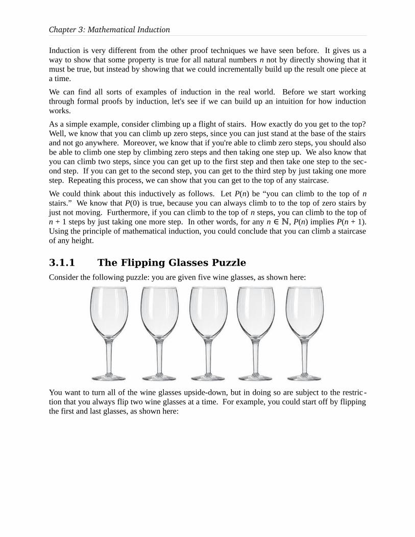
Chapter 3: Mathematical Induction

Induction is very different from the other proof techniques we have seen before. It gives us a way to show that some property is true for all natural numbers n not by directly showing that it must be true, but instead by showing that we could incrementally build up the result one piece at a time.

We can find all sorts of examples of induction in the real world. Before we start working through formal proofs by induction, let's see if we can build up an intuition for how induction works.

As a simple example, consider climbing up a flight of stairs. How exactly do you get to the top? Well, we know that you can climb up zero steps, since you can just stand at the base of the stairs and not go anywhere. Moreover, we know that if you're able to climb zero steps, you should also be able to climb one step by climbing zero steps and then taking one step up. We also know that you can climb two steps, since you can get up to the first step and then take one step to the sec-ond step. If you can get to the second step, you can get to the third step by just taking one more step. Repeating this process, we can show that you can get to the top of any staircase.

We could think about this inductively as follows. Let P(n) be “you can climb to the top of n stairs.” We know that P(0) is true, because you can always climb to to the top of zero stairs by just not moving. Furthermore, if you can climb to the top of n steps, you can climb to the top of n + 1 steps by just taking one more step. In other words, for any n ∈ ℕ, P(n) implies P(n + 1). Using the principle of mathematical induction, you could conclude that you can climb a staircase of any height.

3.1.1 The Flipping Glasses PuzzleConsider the following puzzle: you are given five wine glasses, as shown here:

You want to turn all of the wine glasses upside-down, but in doing so are subject to the restric -tion that you always flip two wine glasses at a time. For example, you could start off by flipping the first and last glasses, as shown here:

77 / 347

And could then flip the second and fourth glasses, like this:

From here, we might flip the first and third glasses to get this setup:

If you play around with this puzzle, though, you'll notice that it's tricky to get all of the wine glasses flipped over. In fact, try as you might, you'll never be able to turn all of the wine glasses over if you play by these rules. Why is that? Figuring the answer out requires a bit of creativity. Let's count how many wine glasses are facing up at each step. Initially, we have five wine glasses facing up. After our first step, we flip two of the wine glasses, so there are now three wine glasses facing up. At the second step, we have several options:

1. Flip over two glasses, both of which are facing up,

2. Flip over two glasses, both of which are facing down, or

3. Flip over two glasses, one of which is facing up and one of which is facing down.

Chapter 3: Mathematical Induction

How many wine glasses will be facing up after this step? In the first case, we decrease the num-ber of wine glasses facing up by two, which takes us down to one glass facing up. In the second case, we increase the number of wine glasses facing up by two, which takes us to five glasses facing up. In the third case, the net change in the number of wine glasses facing up is zero, and we're left with three glasses facing up.

At this point we can make a general observation – at any point in time, each move can only change the number of up-facing wine glasses by +2, 0, or -2. Since we start off with five wine glasses facing up, this means that the number of wine glasses facing up will always be exactly 1, 3, or 5 – all the odd numbers between 0 and 5, inclusive. To solve the puzzle, we need to get all of the wine glasses facing down, which means we need zero wine glasses facing up. But this means that the puzzle has to be impossible, since at any point in time the number of upward-fac-ing wine glasses is going to be odd.

The question now is how we can formalize this as a proof. Our argument is the following:

• The number of upward-facing wine glasses starts off odd.

• At any point, if the number of upward-facing wine glasses is odd, then after the next move the number of upward-facing wine glasses will be odd as well.

The argument here is inherently inductive. We want to prove that the number of glasses starts odd, and that if it starts odd initially it will stay odd forever. There are many ways to formalize the argument, but one idea would be to prove the following for all natural numbers n:

Lemma: For any natural number n, after n moves have been made, the number of upward-facing glasses is an odd number.

The phrasing here says that no matter how many moves we make (say, n of them), the number of upward-facing glasses will be odd. Given this lemma, it's extremely easy to prove that the puz-zle is unsolvable.

So how exactly do we prove the lemma? In a proof by induction, we need to do the following:

1. Define some property P(n) that we want to show is true for all natural numbers n.

2. Show that P(0) is true.

3. Show that for any natural number n, if P(n) is true, then P(n + 1) is true as well.

Let's walk through each of these steps in detail. First, we'll need to come up with our property P(n). Here, we can choose something like this:

P(n) ≡ “After n steps, there are an odd number of upward-facing glasses.”

Notice that our choice of P(n) only asserts that there are an odd number of upward-facing glasses for some specific n. That is, P(4) just says that after four steps, there are an odd number of up-ward-facing glasses, and P(103) just says that after 103 steps, there are an odd number of up-ward-facing glasses. This is perfectly normal in an induction proof. Mathematical induction lets us define properties like this one, then show that the property is true for all choices of natural numbers n. In other words, even though we want to prove that the claim is true for all natural numbers n, our property only says that the claim must be true for some specific choice of n.

79 / 347

Now that we have our property, we need to prove that P(0) is true. In this case, that means that we have to show that after 0 steps, there are an odd number of upward-facing glasses. This is true almost automatically – we know that there are five upward-facing glasses to begin with, and if we make 0 steps we can't possibly change anything. Thus there would have to be five upward-facing glasses at the end of this step, and five is odd.

It seems almost silly that we would have to make this argument at all, but it's crucial in an induc-tive proof. Remember that induction works by showing P(0), then using P(0) to get P(1), then using P(1) to get P(2), etc. If we don't show that P(0) is true, then this entire line of reasoning breaks down! Because the entire inductive proof hinges on P(0), P(0) is sometimes called the inductive basis or the base case.

When writing inductive proofs, you'll often find that P(0) is so trivial that it's almost comical. This is perfectly normal, and is confirmation that your property is not obviously incorrect. Al-ways make sure to prove P(0) in an inductive proof.

The last step in an induction is to show that for any choice of n ∈ ℕ, that if P(n) is true, P(n + 1) must be true as well. Notice the structure of what we need to show – for any choice of n, we must show that P(n) implies P(n + 1). As you saw last chapter, to prove something like this, we'll choose some arbitrary natural number n, then prove that P(n) → P(n + 1). Since our choice of n is arbitrary, this will let us conclude that P(n) → P(n + 1) for any choice of n. In turn, how do we then show that P(n) → P(n + 1)? This statement is an implication, so as we saw last chap-ter, one option is to assume that P(n) is true, then to prove P(n + 1). This step of the proof is called the inductive step, and the assumption we're making, namely that P(n) is true, is called the inductive hypothesis.

If you think about what we're saying here, it seems like we're assuming that for any n, P(n) is true. This is not the case! Instead, what we are doing is supposing, hypothetically, that P(n) is true for one specific natural number n. Using this fact, we'll then go to show that P(n + 1) is true as well. Since the statements P(n) and P(n + 1) are not the same thing, this logic isn't circular.

So we now have the structure of what we want to do. Let's assume that for some arbitrary natu-ral number n ∈ ℕ, that P(n) is true. This means that after n steps, the number of upward-facing glasses is odd. We want to show that P(n + 1) is true, which means that after n + 1 steps, the number of upward-facing glasses is odd. How would we show this? Well, we're beginning with the assumption that after n steps there are an odd number of upward-facing glasses. Let's call this number 2k + 1. We want to assert something about what happens after n + 1 steps, so let's think about what that (n + 1)st step is. As mentioned above, there are three cases:

• We flip two upward-facing glasses down, so there are now 2k + 1 – 2 = 2(k – 1) + 1 up-ward-facing glasses, which is an odd number.

• We flip two downward-facing glasses up, so there are now 2k + 1 + 2 = 2(k + 1) + 1 up-ward-facing glasses, which is an odd number.

• We flip one upward-facing glass down and one downward-facing glass up, which leaves the total at 2k + 1 upward-facing glasses, which is also odd.

So in every case, if after n steps the number of upward-facing glasses is odd, then after n + 1 steps the number of upward-facing glasses is odd as well. This statement, combined with our proof of P(0) from before, lets us conclude by mathematical induction that after any number of steps, the number of upward-facing glasses is odd.

Chapter 3: Mathematical Induction

This line of reasoning can be adapted into a short and elegant formal proof by induction, which is shown here:

Lemma: For any natural number n, after n moves have been made, the number of upward-facing glasses is an odd number.

Proof: By induction. Let P(n) be “after n moves have been made, the number of upward-facing glasses is an odd number.” We prove that P(n) is true for all n ∈ ℕ by induction, from which the lemma follows.

As our base case, we will prove P(0), that after 0 moves have been made, the number of upward-facing glasses is an odd number. After zero moves are made, the glasses are still in their initial configuration. Since we begin with five upward-facing glasses, this means that after 0 moves, the number of upward-facing glasses is five, which is odd.

For our inductive step, assume that for some n ∈ ℕ that P(n) is true and that after n moves have been made, the number of upward-facing glasses is odd. We will prove P(n + 1), that after n + 1 moves have been made, the number of upward-facing glasses is odd. Any se-quence of n + 1 moves consists of a sequence of n moves followed by any single move. So consider any sequence of n moves. By our inductive hypothesis, after these n moves are made, the number of upward-facing glasses is odd; let the number of upward-facing glasses be 2k + 1 for some k . Consider the (∈ ℤ n + 1)st move. This flips two glasses, and there are three cases to consider:

Case 1: We flip two upward-facing glasses down. This means there are now 2k + 1 – 2= 2(k – 1) + 1 upward-facing glasses, which is an odd number.

Case 2: We flip two downward-facing glasses up. This means there are now 2k + 1 + 2= 2(k + 1) + 1 upward-facing glasses, which is an odd number.

Case 3: We flip one downward-facing glass up and one upward-facing glass down. This means there are still 2k + 1 upward-facing glasses, which is an odd number.

Thus in each case, the number of upward-facing glasses after n + 1 steps is an odd number, so P(n + 1) holds. This completes the induction. ■

Take a minute to notice the structure of this proof. As with a proof by contradiction or contra-positive, we begin by announcing that the proof will be by induction. We then define our choice of property P(n) that we will prove correct by induction. Next, we announce that we are going to prove P(0), state what P(0) is, then prove P(0) is true. Having done this, we then announce that we're going to assume that P(n) is true for some choice of natural number n, and mention what this assumption means. We then state that we're going to prove P(n) and what specifically this means that we're going to show. We then use the assumption of P(n) as a starting point to prove P(n + 1), and proceed as in a normal proof. Finally, we conclude the proof by noting that we've

81 / 347

done a legal induction. Although the types of proofs you can do by induction vary greatly (as you'll see in this chapter), the basic structure of an induction proof will almost always follow this general template.

Given this lemma, we can formally prove that the flipping glasses puzzle is unsolvable:

Theorem: The flipping glasses puzzle has no solution.

Proof: By contradiction; suppose there is a solution. If this solution has k steps, then after the kth step, all the glasses must be facing down. By our previous lemma, we know that an odd number of glasses must be facing up. But this is impossible, since if all five glasses are facing down, then zero are facing up, and zero is even. We have reached a contradic-tion, so our assumption must have been wrong. Thus there is no solution to the puzzle. ■

3.2 SummationsOne of the most common applications of induction is in simplifying summations. Summations arise frequently in computer science when analyzing the growth rates of certain algorithms, in combinatorics when determining how many objects there are of certain sizes, etc.

As an example, consider the selection sort algorithm, an algorithm for sorting a list of values into ascending order. The algorithm works based on the following observation. If we remove the smallest element from the list, we know that in the sorted ordering of the list it would appear at the front. Consequently, we can just move that element to the front of the list, then sort what remains. We then move the smallest of the remaining elements to the second-smallest position, the smallest of what remains after that to the third-smallest position, etc. As an example, sup-pose that we want to sort this list of values:

4 1 0 3 2

We begin by removing the zero and putting it in the front of the list:

0 4 1 3 2

Now, we sort what remains. To do this, we find the smallest element of what's left (the 1), re-move it from the list, and place it after the 0:

0 1 4 3 2

Repeating this moves the smallest element (2) to the result:

0 1 2 4 3

We then move the smallest value of what remains (3) to get

0 1 2 3 4

and finally, we move the last element (4) to get the overall sorted sequence

0 1 2 3 4

Chapter 3: Mathematical Induction

How efficient of a sorting algorithm is this? In order to answer this question, we need to find some way to quantify how much work is being done. Once we've done that, we can analyze what that quantity is to determine just how efficient the overall algorithm is.

Intuitively, the selection sort algorithm works as follows;

• While there are still elements left to be sorted:

• Scan across all of them to find the smallest of what remains.

• Append that to the output.

It seems that appending the smallest remaining value to the output is unlikely to take a lot of time (we'll talk about this a bit more later). Scanning over each element to determine which element is smallest, on the other hand, might take quite a bit of time.

As an example, suppose we want to sort one million integers. Using selection sort, we'd begin by scanning over the entire list of one million elements to determine which was the smallest. Once we've done that, we then scan over the 999,999 remaining elements to determine which of them is the smallest. After that, we scan over the 999,998 remaining elements to determine which of them is the smallest, etc. This seems like it's going to take a while, but just how much time is it going to take?

In order to sort a list of n values using selection sort, we need to scan n elements on the first round, then n – 1 on the second, n – 2 on the third, etc. This means that the total number of ele-ments that we're going to scan will be given by

n + (n – 1) + (n – 2) + … + 3 + 2 + 1

What is this value equal to? Well, that depends on our choice of n. If we try this for small val-ues of n, we get the following:

• When n = 1, the sum is equal to 1.

• When n = 2, the sum is 1 + 2 = 3.

• When n = 3, the sum is 1 + 2 + 3 = 6.

• When n = 4, the sum is 1 + 2 + 3 + 4 = 10.

• When n = 5, the sum is 1 + 2 + 3 + 4 + 5 = 15.

Is there some sort of trend here? As with most interesting parts of mathematics, the answer is definitely “yes,” but what exactly is this trend? When confronted with a sequence like this one (1, 3, 6, 10, 15, …) where we can't spot an immediate pattern, there are many techniques we can use to try to figure out what the sum is equal to. In fact, there are entire textbooks written on the subject.

In this case, one option might be to try drawing a picture to see if we can spot anything interest-ing. Suppose that we visualize each of the numbers as some quantity of blocks. We might draw 1 as one block, 2 as two blocks, 3 as three blocks, etc. Suppose that we place all of these blocks next to one another, like this:

83 / 347

+ + + + + =

We now have a nice triangle shape to work with. If this were an actual triangle, we could try us-ing the formula A = ½bh in order to compute the total area here. If we are summing n + (n – 1) + … + 2 + 1, then the base of the triangle has width n and the height has width n as well. Accord-ing to the formula for the area of a triangle, we'd therefore expect the number of blocks to be ½n2. Does this work? Unfortunately, no. The first few values of ½n2 are

0, 0.5, 2, 4.5, 8, 12.5, …

whereas the first few values of the sum of the first n positive natural numbers is

0, 1, 3, 6, 10, 15, …

Why doesn't this reasoning exactly work? Well, if we superimpose a real triangle of width n and height n on top of our boxy triangle, we get this:

As you can see, our boxy triangle extends past the bounds of the real triangle by a small amount. This accounts for why the sum of the first n positive natural numbers is a little bit bigger than n2.

Although this doesn't exactly work out correctly, this geometric line of reasoning is actually quite interesting. Why exactly is the area of a triangle equal to ½bh? One way to derive this is to start with any triangle we like, perhaps this one:

then to draw a box around it, like this:

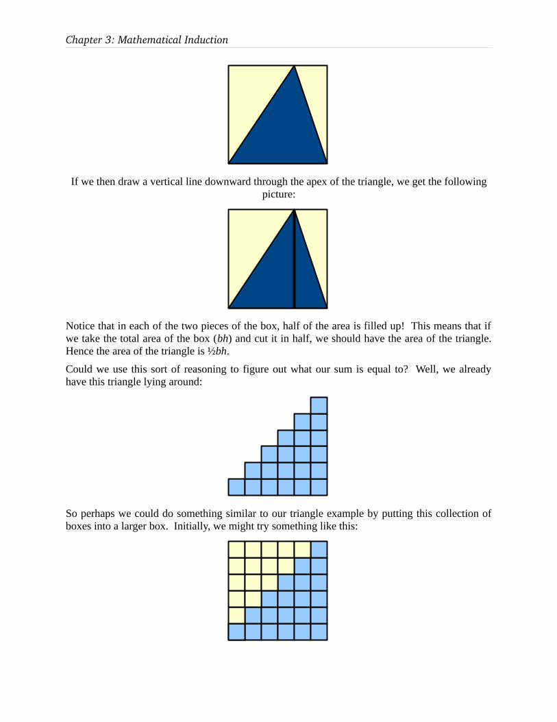
Chapter 3: Mathematical Induction

If we then draw a vertical line downward through the apex of the triangle, we get the following picture:

Notice that in each of the two pieces of the box, half of the area is filled up! This means that if we take the total area of the box (bh) and cut it in half, we should have the area of the triangle. Hence the area of the triangle is ½bh.

Could we use this sort of reasoning to figure out what our sum is equal to? Well, we already have this triangle lying around:

So perhaps we could do something similar to our triangle example by putting this collection of boxes into a larger box. Initially, we might try something like this:

85 / 347

In this picture, we can see that roughly half of the boxes in the large rectangle belong to our sum, while the other half do not. We can therefore get a rough estimate for 1 + 2 + … + n as being about n2. However, this is not an exact figure, because it's not an even split. For example, in the above figure, there are 21 boxes from our original sum, and 15 boxes that we added.

Although the above drawing doesn't exactly work, it's very close to what we want. There are several techniques we can use to fix it. One clever observation we can have is that the boxes we have added form a triangle of width n – 1 and height n – 1, compared to our original triangle, which has width n and height n. Given this, suppose that we pull off the last column of our trian-gle. This gives us the following picture:

This picture gives us a very nice intuition for the sum. If we look at the rectangle on the left, we now have that exactly half of the boxes are from our original sum and exactly half of the boxes are from the completion. This box has width n – 1 and height n, so of the n(n – 1) total boxes, one-half of them are from the original sum. We also have one final column from our original sum, which has n boxes in it. This means that we might expect 1 + 2 + … + n to be equal to

n(n−1)

2+ n=

n(n−1)

2+

2 n2

=n(n−1)+ 2 n

2=

n(n−1+ 2)

2=

n(n+ 1)

2

Indeed, if we check the first few terms of n(n + 1) / 2, we end up getting the sequence

0, 1, 3, 6, 10, 15, 21, ...

which matches our values for 0, 1, 1 + 2, 1 + 2 + 3, etc.

A different way of manipulating our diagram would be to change how we add in the extra boxes. If instead of creating a square, we create this rectangle:

then we can see that exactly half of the squares in this rectangle are used by our triangle. Since this rectangle has area n(n + 1), this means that the sum of the first n positive natural numbers should probably be n(n + 1) / 2, which agrees with our previous answer.

Chapter 3: Mathematical Induction

One final way we can think about the geometric intuition is to abandon the idea of completing the rectangle and to instead return to this earlier drawing, in which we superimposed the real tri-angle width and height n on top of our boxy triangle:

As before, one idea might be to treat the total area of the boxes as the sum of two different areas – the area covered by the triangle, and the area filled by the pieces of the boxes extending above the triangle. If our triangle has width n and height n, then there will be n smaller triangles ex-tending beyond the n by n triable. Each of these triangles has width 1 and height 1, and therefore has area ½. Consequently, the total area taken up by our boxes would be given by the total area of the large triangle, plus n copies of the smaller triangle. This is

n2

2+

n2=

n2+ n2

=n(n+ 1)

2

And again we've reached the same result as before!

The takeaway point from this is that there are always different ways of thinking about problems in mathematics. You might end up at the same result through several different paths, each of which casts light on a slightly different angle of the problem.

So the big question is how this has anything to do with induction at all. Well, at this point we have a pretty good idea that the sum of the first n positive natural numbers is going to ben(n + 1) / 2. But how would we rigorously establish this? Here, induction can be invaluable. We can prove that the above sum is correct by showing that it's true when n = 0, and then show-ing that if the sum is true for some choice of n, it must be true for n + 1 as well. By the principle of mathematical induction, we can then conclude that it must be true for any choice of n.

Here is one possible proof:

Theorem: The sum of the first n positive natural numbers is n(n + 1) / 2.

Proof: By induction. Let P(n) be “the sum of the first n positive natural numbers isn(n + 1) / 2.” We prove that P(n) is true for all n ∈ ℕ, from which the result immediately follows.

For our base case, we prove P(0), that the sum of the first 0 positive natural numbers is0(0 + 1) / 2. The sum of zero numbers is 0, and 0 = 0(0 + 1)/2. Consequently, P(0) holds.

87 / 347

For the inductive step, assume that for some n ∈ ℕ that P(n) is true and the sum of the first n positive natural numbers is n(n + 1) / 2. We will prove that P(n + 1) is true; that is, the sum of the first n + 1 positive natural numbers is (n + 1)(n + 2) / 2. Consider the sum of the first n + 1 positive natural numbers. This is the sum of the first n positive natural numbers, plus n + 1. By our inductive hypothesis, the sum of the first n positive natural numbers is n(n + 1) / 2. Thus the sum of the first n + 1 positive natural numbers is

n(n+ 1)

2+ n+ 1=

n(n+ 1)

2+

2(n+ 1)

2=

n(n+ 1)+ 2 (n+ 1)

2=

(n+ 2)(n+ 1)

2

Thus P(n + 1) is true, completing the induction. ■

What a trip this has been! We began by asking how efficient the selection sort algorithm was. In doing so, we made a detour into geometry to build up an intuition for the answer, and then used induction to formalize the result.

So back to our original question – how efficient is selection sort? Answer: not very. Selection sorting n elements requires us to scan a total of n(n + 1) / 2 elements in the course of completing the algorithm. Plugging in n = 1,000,000 gives us that we will make 500,000,500,000 scans. That's 500 billion element lookups! Even a processor operating in the gigahertz will take a while to finish sorting that way.

The beauty of the result that we have just proven, though, is that from this point forward if we ever see an algorithm that has this sort of behavior we immediately know how much work it will have to do.

3.2.1 Summation NotationIn the previous section, we considered the sum

1 + 2 + … + (n – 1) + n

In the course of the proof, we kept referring to this sum as “the sum of the first n positive natural numbers.” This is a fairly long-winded way of explaining what sum we're computing, and it would be nice if there were a simpler way to do this.

When working with summations, mathematicians typically use Σ notation to describe the sum more compactly. Rather than writing out a sequence with an ellipsis in the middle, we instead describe a general formula for each individual term being summed together, then specify how many terms we want to sum up.

In general, we can describe the sum of a1 + a2 + … + an as follows:

∑i=1

n

ai

Let's piece this apart to see what it says. The large Σ indicates that we are looking at the sum of some number of terms. The values below and above the Σ tell us over what values the summa-tion ranges. Here, the sum ranges from i = 1 to n, so we will sum up over the terms inside the

Chapter 3: Mathematical Induction

sum when i = 1, i = 2, i = 3, etc. up to and including when i = n. Finally, we have the values ac-tually being summed together. Here these are the values ai. As i ranges from 1 to n, we will ag-gregate and sum up all of these terms.

More formally:

∑i=m

n

ai is the sum of all ai where i ∈ ℕ and m ≤ i ≤ n.

For example, let's consider our original sum 1 + 2 + … + n. We can write this sum as

∑i=1

n

i

This says that we should sum up i as i ranges from 1 up to and including n. For example, if we pick a specific n (say, n = 5), then we have that

∑i=1

5

i=1+ 2+ 3+ 4+ 5

If you are coming from a programming background, you can think of the summation as a sort of mathematical “for loop” that ranges over choices of i and sums up the values that are listed.

Summations can have more complex bounds. For example, we could write the sum (-3) + (-2) + (-1) + 0 + 1 as

∑i=−3

1

i=(−3)+ (−2)+ (−1)+ 0+ 1

or could sum from 0 to 4 as

∑i=0

4

i=0+ 1+ 2+ 3+ 4

In addition to changing the loop bounds, we can also change what's inside the summation actu-ally getting added up. For example, suppose that we wanted to sum up the first n perfect cubes (that is, 03 + 13 + 23 + …). We could write this as follows:

∑i=0

n−1

i 3=03+ 13+ 23+ ...+ (n−1)3

There are two important details to note here. First, note that the upper bound on the sum is n – 1, not n, even though we're summing up the first n perfect cubes. The reason for this is that the lower bound of the summation is 0, not 1. This means that there are a total of n elements being summed up, not n – 1. Second, notice that the value being summed this time is not i, but i3. In general, we can perform any arbitrary manipulations of the index of summation inside the sum. We could, for example, sum up powers of two this way:

∑i=0

n−1

2i=20

+ 21+ 22

+ 23+ ...+ 2n−1

89 / 347

When working with induction, one special kind of sum arises with surprising frequency. Con-sider what happens when we have a sum like this one:

∑i=1

0

ai

Notice that this sum is the sum from i = 1 to 0. What is the value of this sum? In this case, the sum doesn't include any numbers. We call sums like this one – where no values are being added up – empty sums. It is specified here:

A sum of no numbers is called the empty sum and has value 0.

Thus all of the following sums are empty sums and therefore equal to zero:

∑i=1

0

2i=0 ∑i=137

42

(i+ 1)=0 ∑i=−1

−2

i=0 ∑i=5

0

i i=0

However, note that the following sum is not empty:

∑i=0

0

2i

Since the indices of summation are inclusive, this means that this sum includes the term where i = 0. Consequently, this sum is equal to 20 = 1.

Empty sums may seem like little more than a curiosity right now, but they appear frequently in the base cases of inductive proofs.

Now that we have a formal notation we can use to manipulate sums, let's return back to our pre-vious inductive proof. We proved that 1 + 2 + … + n = n(n + 1) / 2. What might this look like using summations? Well, we can rewrite the sum 1 + 2 + … + n as

∑i=1

n

i

Consequently, we can restate the theorem we have just proven as follows:

∑i=1

n

i=n(n+ 1)

2

Let's repeat our previous proof, this time using summation notation. From this point forward, we will almost exclusively use summation notations in formal proofs involving sums.

Theorem: For any n ∈ ℕ, ∑i=1

n

i=n(n+ 1)

2.

Chapter 3: Mathematical Induction

Proof: By induction. Let P(n) be defined as

P (n)≡∑i=1

n

i=n (n+ 1)

2We prove that P(n) is true for all n ∈ ℕ by induction on n. As our base case, we prove P(0), that is, that

∑i=1

0

i=0(0+ 1)

2The left-hand side of this equality is the empty sum, which is 0. The right-hand side of the equality is also 0, so P(0) holds.

For the inductive step, assume that for some natural number n, P(n) holds, meaning that

∑i=1

n

i=n(n+ 1)

2We will prove P(n + 1), meaning that

∑i=1

n+ 1

i=(n+ 1)(n+ 2)

2To see this, note that

∑i=1

n+ 1

i=∑i=1

n

i+ n+ 1=n (n+ 1)

2+ n+ 1=

n(n+ 1)+ 2(n+ 1)

2=

(n+ 2)(n+ 1)

2Thus P(n + 1) holds, completing the induction. ■

One of the key steps in this proof was recognizing that

∑i=1

n+ 1

i=∑i=1

n

i+ n+ 1

Why does this step work? Well, the left-hand side is the sum of the first n + 1 positive natural numbers. The right-hand side is the sum of the first n positive natural numbers, plus n + 1, the (n + 1)st positive natural number. All that we've done is “peel off” the last term of the sum to make it a bit easier to work with. This technique arises in many inductive proofs, since in order to reason about the sum of the first n + 1 terms of a series it may help to consider the sum of the first n terms of the series, plus the (n + 1)st term by itself.

3.2.2 Summing Odd NumbersNow that we have a framework for manipulating sums of numbers, let's do some exploration and see if we can find some other interesting sums to explore.

What happens if we start adding together the first n odd numbers? If we do this, we'll find the following:

91 / 347

• The sum of the first 0 odd numbers is 0. It's an empty sum.

• The sum of the first 1 odd numbers is 1.

• The sum of the first 2 odd numbers is 1 + 3 = 4.

• The sum of the first 3 odd numbers is 1 + 3 + 5 = 9.

• The sum of the first 4 odd numbers is 1 + 3 + 5 + 7 = 16.

Now that's surprising... the first five terms of this sequence are 0, 1, 4, 9, 16 = 02, 12, 23, 32, 42. Does this trend continue? If so, could we prove it? One of the beautiful consequences of mathe-matical induction is that once you have spotted a trend, you can sit down and attempt to prove that it is not a coincidence and in fact continues for all natural numbers. Even if we don't have an intuition for why the sums of odd numbers might work out this way, we can still prove that they must.

Let's see how a proof of this fact might work. First, we have to figure out what we want to show. Our goal is to show that the sum of the first n odd numbers is equal to n2. How would we phrase this as a summation? Well, we know that the odd numbers are numbers of the form 2k + 1 for in-tegers k, so one way of phrasing this sum would be

∑i=0

n−1

(2 i+ 1)

Notice that the summation ranges from i = 0 to n – 1, so the sum has n terms in it. It seems like this might cause a problem when n = 0, since then the sum ranges from 0 to -1. However, this is nothing to worry about. When n = 0, we don't want to sum anything up (we're talking about the sum of no numbers), and if we try evaluating a sum ranging from 0 to -1 we are evaluating an empty sum, which is defined to be 0.

Given this setup, let's try to prove that the sum of the first n odd numbers is n2.

Theorem: For any natural number n, ∑i=0

n−1

(2 i+ 1)=n2 .

Proof: By induction. Let P(n) be defined as

P (n)≡∑i=0

n−1

(2 i+ 1)=n2

We prove that P(n) is true for all n ∈ ℕ by induction on n. As our base case, we prove P(0), that is, that

∑i=0

−1

(2 i+ 1)=02

The left-hand side of this equality is the empty sum, which is 0. The right-hand side of the equality is also 0, so P(0) holds.

Chapter 3: Mathematical Induction

For the inductive step, assume that for some natural number n, P(n) holds, meaning that

∑i=0

n−1

(2 i+ 1)=n2

We will prove P(n + 1), meaning that

∑i=0

n

(2 i+ 1)=(n+ 1)2

To see this, note that

∑i=0

n

(2 i+ 1)=(n+ 1)2=∑i=0

n−1

(2i+ 1)+ 2 n+ 1=n2+ 2n+ 1=(n+ 1)2

Thus P(n + 1) holds, completing the induction. ■

Here, the last step is a consequence of the fact that (n + 1)2 expands out to n2 + 2n + 1.

So we now have a mathematical proof of the fact that the sum of the first n odd natural numbers is equal to n2. But why is this? It's here that we see one shortcoming of induction as a technique. The above proof gives us almost no intuition as to why the result is correct.

We might then ask – so why is that true? As with our proof about the sum of the first n positive natural numbers, it might help to draw a picture here. Suppose we start adding up odd numbers, like this:

+ + + + + =

There isn't an immediate pattern here, but using the same intuition we had for the sum of the first n natural numbers we might try completing this second rectangle to form some box:

93 / 347

What are the dimensions of this larger box? Since there are n odd numbers being summed up, the height of the box is n. The width of the box is one plus the largest odd number being added up. If we look at our summation, we note that we're adding up terms of the form 2i + 1 and stop when i = n – 1. Plugging in i = n – 1 to get the largest odd number added up, we get 2(n – 1) + 1 = 2n – 2 + 1 = 2n – 1. Since the width of the box is one more than this, we end up seeing that the width of the box is 2n. Thus the box has dimensions n by 2n, so its area is 2n2. Since half of that area is used up by the boxes for our sum, the sum should be equal to n2, as we saw before.

But this is just one intuition for the result. Let's look at our triangle one more time. We already know from before what the area of this highlighted triangle is:

This is the triangle we drew when we were considering the sum of the first n positive natural numbers. So what remains in this picture? Well, notice that in the first row there are 0 blue squares, in the second row there is one blue square, in the third there are two blue squares, etc. In fact, the number of total blue squares is 1 + 2 + … + n – 1. We can see this by rearranging the above digram like this:

This means that the sum of the first n odd numbers is the sum of the first n positive natural num-bers, plus the sum of the first n – 1 positive natural numbers. We happen to have formulas for these sums. If we add them together, we get the following:

n(n+ 1)

2+

(n−1)n2

=n(n+ 1)+ n(n−1)

2=

n(n+ 1+ n−1)

2=

n(2n )

2=

2n2

2=n2

Et voilà! We have our result.

But it turns out that with the above picture there's a much easier way of arriving at the result. What happens if we rotate the blue triangle 180 degrees? If we do this, we'll end up getting this picture:

Chapter 3: Mathematical Induction

The total area of this square is equal to the sum of the first n odd numbers. Since the square has size n × n, the sum of the first n odd numbers should be n2, as it indeed is.

Of course, none of these intuitions match the intuition that we actually used in our proof. Let's revisit the proof for a short while to see if we can come up with a different explanation for why the result is true.

We can get a bit of an intuition from looking at the last step of the proof. If you'll notice, the proof works because given n2, adding in 2n + 1 (the (n + 1)st odd number) takes us up to (n + 1)2. In other words, we have that

(n + 1)2 – n2 = n2 + 2n + 1 – n2 = 2n + 1

So one reason to think that this result would be true is that the spacing between consecutive pow-ers of two is always an odd number. If we keep adding up odd numbers together over and over again, we thus keep advancing from one term in the sequence to the next.

But why exactly is that? It turns out that, again, there is a beautiful geometric intuition. Suppose that we have the sum of the first n odd numbers, which we know is equal to n2. We can draw this as follows:

Now, suppose that we add in the (n + 1)st odd number, which is 2n + 1. One way to visualize what happens when we do this is to break the 2n + 1 apart into three pieces – one piece of size n, one piece of size n, and one piece of size 1. Doing so gives us the following:

95 / 347

As you can see, these three pieces can be added to the square in a way that extends it into a square of the next size. This in a sense justifies our induction. The reason that the sum of the first n odd numbers is equal to n2 is because each odd number contributes enough to the previous perfect square to get us up to the next perfect square.

This intuition is actually extremely powerful, and we can use it as a stepping stone toward a larger result. The key idea is to think about what we just did backwards. Here, we started off with the sum of the first n odd numbers and ended up with the perfect squares. But in reality, our proof works the other way. We showed that you can progress from one perfect square to the next by adding in the (n + 1)st odd number. This was almost a pure coincidence – it wasn't the fact that it was the (n + 1)st odd number so much as it was the value 2n + 1, which is the difference between two adjacent terms in the sequence. The fact that we call numbers of the form 2n + 1 the odd numbers was entirely accidental.

3.2.3 Manipulating SummationsAny good mathematical proof can be lifted into a more general setting, as you will see repeatedly throughout your exploration of the mathematical foundations of computing. The proof we just completed about sums of odd numbers can indeed be generalized to a more elaborate and more powerful result that we can use to derive all sorts of results without having to directly resort to induction.

Before jumping off, let's review something that we already happened to know. We currently know a formula for the sum of the first n positive integers; specifically, we have that

∑i=1

n

i=n(n+ 1)

2

Let's update this so that we have this formula phrased in terms of the sum of the first n natural numbers, rather than positive integers. If we consider this value, we get the sum

∑i=0

n−1

i

What is the value of this sum? Well, one thing we can note is the following:

∑i=0

n−1

i=∑i=0

n−1

i+ n−n=∑i=0

n

i−n

Now, we can exploit the fact that this first sum is equal to 0 + 1 + 2 + … + n. This has exactly the same value as 1 + 2 + … + n, because the zero doesn't contribute anything. In other words, we can just restart this summation at 0 rather than at 1 without changing the value of the expres-sion. This gives us

∑i=0

n−1

i=∑i=0

n

i−n=∑i=1

n

i−n=n(n+ 1)

2−n=

n(n+ 1)−2n2

=n (n+ 1−2)

2=

n (n−1)

2

In other words, we have just shown that

∑i=0

n−1

i=n(n−1)

2

Chapter 3: Mathematical Induction

This formula is extremely important – you should definitely commit it to memory!

What we have just done right here was derive a new result about a summation based off an old result about summations. Most of the time that you need to evaluate summations, you can use standard techniques like these to get a nice value for the summation without having to draw pic-tures or use induction. This section focuses on some standard identities you can use to simplify summations, along with the proofs of why they work. In a sense, the proofs that we will do here will serve as lemmas that we can use later on when simplifying sums we have never seen before. Although most of the proofs here may seem obvious, it's good to justify that they always work correctly.

Right now, we have a nice closed-form solution for the sum of the first n natural numbers. More explicitly, we have this:

∑i=0

n−1

i 1=n(n−1)

2

I've explicitly highlighted the fact that we're computing 01 + 11 + 21 + … + (n – 1)1. What if we were to change the exponent? What effect would this have on the sum?

One simple change would be to set the exponent to 0, meaning we'd be computing 00 + 10 + 20 + … (n – 1)0 = 1 + 1 + … + 1.* This should come out to n, since we're adding 1 up n times. This is indeed the case, as seen in this proof:

Theorem: For any natural number n, ∑i=0

n−1

1=n .

Proof: By induction. Let P(n) be defined as

P (n)≡∑i=0

n−1

1=n

We prove that P(n) is true for all n ∈ ℕ by induction on n. As our base case, we prove P(0), that is, that

∑i=0

−1

1=0

The left-hand side of this equality is the empty sum, which is 0. The right-hand side of the equality is also 0, so P(0) holds.

For the inductive step, assume that for some natural number n, P(n) holds, meaning that

∑i=0

n−1

1=n

We will prove P(n + 1), meaning that

* This assumes that 00 = 1.  In most of discrete mathematics, this is a perfectly reasonable assumption to make, and we will use this convention throughout this course.

97 / 347

∑i=0

n

1=n+ 1

To see this, note that

∑i=0

n

1=∑i=0

n−1

1+ 1=n+ 1

Thus P(n + 1) holds, completing the induction. ■

This proof might seem silly, but it's good to be able to confirm results that we intuitively know to be true. This gives us a nice starting point for future work.

So we now know how to sum up n0 and n1 from zero forward. What other sums might we be in-terested in simplifying? One thing we might do at this point would be to revisit our earlier proof about sums of odd numbers. We proved explicitly by induction that

∑i=0

n−1

(2 i+ 1)=n2

Could we somehow prove this result without using induction? Here is one possible approach that we might be able to use. Right now we know how to sum up n0 (1) and n1 (n). Could we perhaps decompose this sum into these two pieces?

∑i=0

n−1

(2 i+ 1)=∑i=0

n−1

2 i+∑i=0

n−1

1

We already know a value for the second term, since we explicitly proved that this sum is equal to n. This means that we have

∑i=0

n−1

(2 i+ 1)=∑i=0

n−1

2 i+ n

It seems like we also should be able to simplify the first sum like this:

∑i=0

n−1

(2 i+ 1)=2∑i=0

n−1

i+ n

From there, we can use our formula for the second sum to get

∑i=0

n−1

(2 i+ 1)=2n(n−1)

2+ n=n (n−1)+ n=n2−n+ n=n2

And we have an entirely new proof of the fact that the sum of the first n odd numbers is equal to n2. But unfortunately, this proof makes two intuitive leaps that we haven't yet justified. First, why can we split the initial sum up into two separate sums? Second, why can we factor a con -stant out of the sum? Both of these steps are reasonable because of properties of addition, but are we sure they work for the general case? The answer turns out to be “yes,” so the above proof is valid, but let's take a minute to prove each of these.

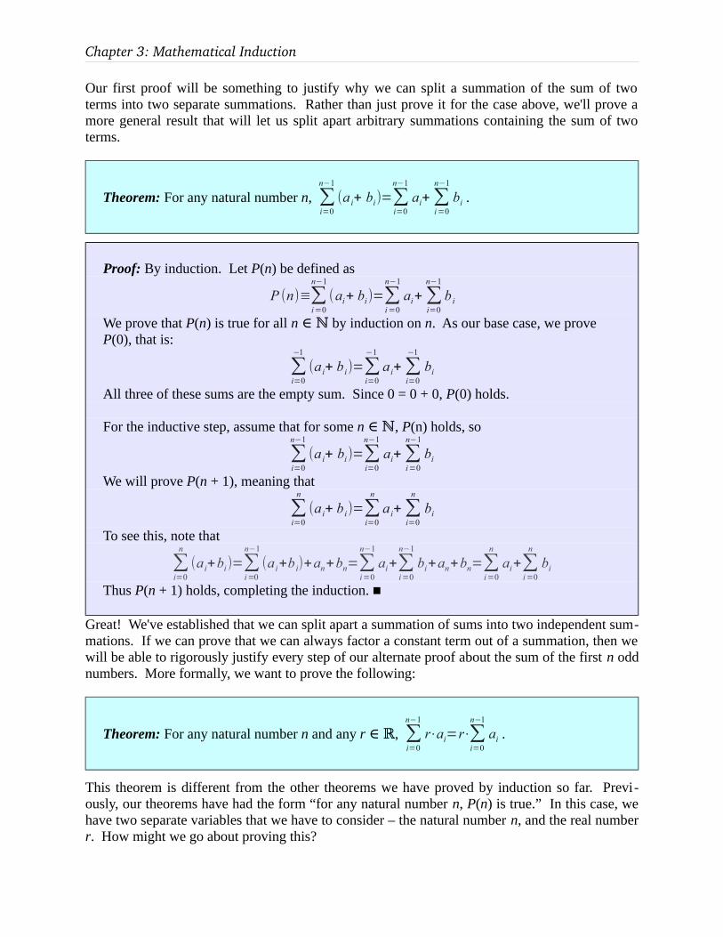
Chapter 3: Mathematical Induction

Our first proof will be something to justify why we can split a summation of the sum of two terms into two separate summations. Rather than just prove it for the case above, we'll prove a more general result that will let us split apart arbitrary summations containing the sum of two terms.

Theorem: For any natural number n, ∑i=0

n−1

(a i+ bi)=∑i=0

n−1

ai+ ∑i=0

n−1

bi .

Proof: By induction. Let P(n) be defined as

P (n)≡∑i=0

n−1

(ai+ bi)=∑i=0

n−1

ai+ ∑i=0

n−1

b i

We prove that P(n) is true for all n ∈ ℕ by induction on n. As our base case, we prove P(0), that is:

∑i=0

−1

(a i+ b i)=∑i=0

−1

a i+ ∑i=0

−1

bi

All three of these sums are the empty sum. Since 0 = 0 + 0, P(0) holds.

For the inductive step, assume that for some n ∈ ℕ, P(n) holds, so

∑i=0

n−1

(a i+ bi)=∑i=0

n−1

ai+ ∑i=0

n−1

bi

We will prove P(n + 1), meaning that

∑i=0

n

(a i+ b i)=∑i=0

n

a i+ ∑i=0

n

bi

To see this, note that

∑i=0

n

(a i+bi)=∑i=0

n−1

(a i+b i)+an+bn=∑i=0

n−1

ai+∑i=0

n−1

bi+an+bn=∑i=0

n

ai+∑i=0

n

bi

Thus P(n + 1) holds, completing the induction. ■

Great! We've established that we can split apart a summation of sums into two independent sum-mations. If we can prove that we can always factor a constant term out of a summation, then we will be able to rigorously justify every step of our alternate proof about the sum of the first n odd numbers. More formally, we want to prove the following:

Theorem: For any natural number n and any r , ∈ ℝ ∑i=0

n−1

r⋅ai=r⋅∑i=0

n−1

ai .

This theorem is different from the other theorems we have proved by induction so far. Previ-ously, our theorems have had the form “for any natural number n, P(n) is true.” In this case, we have two separate variables that we have to consider – the natural number n, and the real number r. How might we go about proving this?

99 / 347

Remember that we write a proof by induction by choosing some property P(n), then proving that P(n) is true for all n ∈ ℕ. What if we chose our property P(n) such that if P(n) holds true for all n ∈ ℕ, the overall theorem is true as well? Specifically, since we want our result to work for all n ∈ ℕ and for all r , what if we chose our property ∈ ℝ P(n) as follows:

P(n) ≡ “For all r , ∈ ℝ ∑i=0

n−1

r⋅ai=r⋅∑i=0

n−1

ai ”

Now, if P(n) is true for all natural numbers n, then we must have that for any real number r, we can factor r out of a summation.

Given this, let's see what a proof of the theorem might look like:

Proof: By induction. Let P(n) be defined as

P (n)≡for any r∈R ,∑i=0

n−1

r⋅ai=r⋅∑i=0

n−1

a i

We prove that P(n) is true for all n ∈ ℕ by induction on n. As our base case, we prove P(0), that is, that for any r ,∈ ℝ

∑i=0

−1

r⋅ai=r⋅∑i=0

−1

ai

Both of these sums are the empty sum, and we have that 0 = r · 0 for all r ∈ . Thus ℝ P(0) holds.

For the inductive step, assume that for some n ∈ ℕ, P(n) holds, so for any r ∈ :ℝ

∑i=0

n−1

r⋅ai=r⋅∑i=0

n−1

ai

We will prove P(n + 1), meaning that for any r , we have∈ ℝ

∑i=0

n

r⋅ai=r⋅∑i=0

n

ai

To see this, consider any r . Then∈ ℝ

∑i=0

n

r⋅ai=∑i=0

n−1

r⋅ai+ r⋅an=r⋅∑i=0

n−1

a i+ r⋅an=r (∑i=0

n−1

ai+ an)=r∑i=0

n

an

Thus P(n + 1) holds, completing the induction. ■

We now have four results we can use when trying to prove results about sums:

1. ∑i=0

n−1

1=n

2. ∑i=0

n−1

i=n(n−1)

2

3. ∑i=0

n−1

(a i+ bi)=∑i=0

n−1

ai+ ∑i=0

n−1

bi

4. ∑i=0

n−1

r⋅ai=r⋅∑i=0

n−1

ai

Chapter 3: Mathematical Induction

These four results make it possible to quickly evaluate many useful sums without having to re-sort to induction. For example, suppose that we want to evaluate the following sum, which rep-resents the sum of the first n even natural numbers:

∑i=0

n−1

2 i

We can just compute this directly:

∑i=0

n−1

2 i=2∑i=0

n−1

i=2n (n−1)

2=n(n−1)=n2

−n

This saves us the effort of having to even evaluate a few terms of the series to see if we can spot any trends! We immediately know the answer. To verify that it's correct, let's plug in a few terms to see if it matches our expectation:

• The sum of the first 0 even numbers is 0, and 02 – 0 = 0.

• The sum of the first 1 even number is 0, and 12 – 1 = 1..

• The sum of the first 2 even numbers is 0 + 2 = 2, and 22 – 2 = 2.

• The sum of the first 3 even numbers is 0 + 2 + 4 = 6, and 32 – 3 = 6.

• The sum of the first 4 even numbers is 0 + 2 + 4 + 6 = 12, and 42 – 4 = 12.

It's amazing how much simpler it is to analyze summations this way!

3.2.4 Telescoping SeriesWe now have some general techniques that we can use to manipulate summations. We are about to see a simple but powerful technique that makes it possible to evaluate more complex summa-tions than before – telescoping series.

Earlier in this chapter, we saw that the sum of the first n odd numbers was n2. We saw several ways to prove this, but the particular inductive approach we used was based on the fact that the difference of two consecutive perfect squares is an odd number. In fact, the odd numbers can be thought of as the differences between consecutive perfect squares.

The key insight we needed to have was that (n + 1)2 – n2 = 2n + 1. Given that this is true, let's re-visit our formula for the sum of the first n perfect squares. The initial summation is

∑i=0

n−1

(2 i+ 1)

Now, from above, we have that 2i + 1 = (i + 1)2 – i2. As a result, we can replace the term 2i + 1 in the summation with the expression (i + 1)2 – i2. What happens if we do this? In that case, we get this summation:

∑i=0

n−1

((i+ 1)2−i 2)

If we expand this sum out, something amazing starts to happen. Here's the sum evaluated when n = 0, 1, 2, 3, and 4:

101 / 347

∑i=0

−1

((i+ 1)2−i 2

)=0

∑i=0

0

((i+ 1)2−i 2

)=(12−02

)=1

∑i=0

1

((i+ 1)2−i 2

)=(22−12

)+ (12−02

)=22−02

=4

∑i=0

2

((i+ 1)2−i 2

)=(32−22

)+ (22−12

)+ (12−02

)=32−02

=9

∑i=0

3

((i+ 1)2−i 2

)=(42−32

)+ (32−22

)+ (22−12

)+ (12−02

)=42−02

=16

Notice what starts to happen as we expand out these summations. Each term in the sum is a dif-ference of two terms, where the second term of difference is the first term of the next difference. As a result, all of the inner terms completely disappear, and we're left with the difference of the first term and the last term.

One quick formalism:

The sum ∑i=0

n−1

(x i+ 1− x i) is called a telescoping series.

If we evaluate this sum, then the adjacent pairs will continuously collapse and eventually all that will remain are the first and last elements. We can formally prove this here:

Theorem: For all natural numbers n, ∑i=0

n−1

(x i+ 1− x i)= xn− x0

Proof: By induction. Let P(n) be defined as

P (n)≡∑i=0

n−1

( x i+ 1−xi)=x n−x0

We prove that P(n) is true for all n ∈ ℕ by induction on n. As our base case, we prove P(0), that is:

∑i=0

−1

(x i+ 1− xi)= x0−x0

In this case, the left-hand side is the empty sum and the right-hand side is zero, so P(0) holds.

For the inductive step, assume that for some n ∈ ℕ, P(n) holds, so

∑i=0

n−1

(x i+ 1− x i)=xn− x0

Chapter 3: Mathematical Induction

We will prove P(n + 1), meaning

∑i=0

n

(x i+ 1− xi)= xn+ 1−x0

To see this, notice that

∑i=0

n

(x i+ 1− xi)=∑i=0

n−1

( x i+ 1−xi)+ x n+1−xn=(xn+ 1− xn)+ ( xn−x0)=x n+1−x0

Thus P(n + 1) holds, completing the induction. ■

This result might not initially seem very important, but combined with our previous results we can now solve various summations that we previously would not be able to. For example, we happen to know the value of the following sums:

∑i=0

n−1

1=n ∑i=0

n−1

i=n(n−1)

2

What is the value of the following sum?

∑i=0

n−1

i 2

If we start expanding out some terms, we get the following sequence:

0, 1, 5, 14, 30, 55, …

It's hard to spot a pattern here. If we turn to geometry, we'll find that it's surprisingly tricky to get a good solid geometric intuition for this sum. What other tricks can we try?

Previously, we considered the difference of (n + 1)2 and n2 to learn something about sums of odd numbers. Now, let's suppose that we didn't already know the fact that the sum of the first n natu-ral numbers is n(n – 1) / 2. We could have figured this out as follows. Using properties of tele-scoping sums, we know that

∑i=0

n−1

((i+1)2−i2)=n2

If we simplify the inside of this sum, we get that

∑i=0

n−1

((i+1)2−i2)=∑i=0

n−1

(i2+2i+1−i 2)=∑i=0

n−1

(2i+1)=n2

Now, using properties of summations, we can simplify this as follows:

n2=∑

i=0

n−1

(2i+ 1)=2∑i=0

n−1

i+ ∑i=0

n−1

1

We can replace this final sum with n, which we already know, to get

n2=2∑i=0

n−1

i+ n

If we subtract n from both sides and divide by two, we get

103 / 347

n2−n2

=∑i=0

n−1

i

Since we know that n2 – n = n(n – 1), we have just derived the formula for the sum of the first n natural numbers in a completely different way.

The reason that this derivation is important is that we can use an almost identical trick to deter-mine the sum of the first n perfect squares. The idea is as follows. When working with the dif-ference (n + 1)2 – n2, we were able to derive the formula for the sum of the natural numbers raised to the first power. What happens if we try considering the difference (n + 1)3 – n3? Well, using what we know about telescoping series, we can start off like this:

∑i=0

n−1

((i+ 1)3−i3

)=n3

Since (i + 1)3 – i3 = i3 + 3i2 + 3i + 1 – i3 = 3i2 + 3i + 1, this means that

∑i=0

n−1

(3i2+ 3i+ 1)=n3

Using the properties that we just developed, we can split our sum into three sums:

3∑i=0

n−1

i2+ 3∑

i=0

n−1

i+ ∑i=0

n−1

1=n3

We already know values for these last two sums, so let's go simplify them:

3∑i=0

n−1

i2+3n (n−1)

2+ n=n3

If we now try to isolate the mystery sum, we get the following:

3∑i=0

n−1

i2=n3−3n (n−1)

2−n

∑i=0

n−1

i 2=n3

3−

n(n−1)2

−n3

All that's left to do now is to simplify the right-hand side to make it easy to read:

∑i=0

n−1

i 2=n3

3−

n(n−1)2

−n3=

2n3

6−

3n(n−1)

6−

2n6

=2n3

−3n (n−1)−2n6

=n(2n2

−3(n−1)−2)6

=n (2n2

−3n+ 3−2)

6=

n(2n2−3n+ 1)

6

=n(n−1)(2n−1)

6

And so we can conclude (correctly) that

∑i=0

n−1

i 2=

n(n−1)(2n−1)6

Chapter 3: Mathematical Induction

The beauty of building up all of this machinery is that we don't need to do any induction at all to prove that this result is correct. We have arrived at this result purely by applying theorems that we have developed earlier. The key insight – treating odd numbers as the difference of adjacent perfect squares – is a very powerful one, and using techniques similar to what we've developed above it's possible to find formulas for the sum of the first n kth powers of natural numbers for any arbitrary natural number k.

So far, we have restricted ourself to using telescoping sums to reason about summations of terms of the form xn for some n. That is, we have sums of x0, x1, and x2. But we can come up with summations for other sequences as well. For example, consider the series of powers of two: 20, 21, 22, 23, … = 1, 2, 4, 8, … . We might consider what happens when we start summing these numbers together. For example, we have the following:

∑i=0

−1

((i+1)2−i2)=0

∑i=0

0

2i=1

∑i=0

1

2i=1+ 2=3

∑i=0

2

2i=1+ 2+ 4=7

∑i=0

3

2i=1+2+4+8=15

Can we spot a pattern here? Well, the sequence 0, 1, 3, 7, 15, … is one less than the sequence 1, 2, 4, 8, 16, …; that is, the actual sequence of powers of two. That's interesting... does the trend continue?

It turns out that the answer is yes. We could prove this by using a brand-new induction, but there's a much simpler and more direct way to accomplish this. Using our idea of manipulating telescoping series, we have the following:

∑i=0

n−1

(2i+ 1−2i)=2n−20=2n−1

So what is 2i+1 – 2i? Well, doing some simple algebra tells us that

2 i+ 1−2i

=2 (2i)−2i

=2i

Using this, we can simplify the above summation to get

∑i=0

n−1

(2i+ 1−2i)=∑i=0

n−1

2i=2n−1

So the sum of the first n powers of 2 is 2n – 1. Amazing!

But why stop here? What happens if we sum up 30 + 31 + 32 + … + 3n-1? Do we get 3n – 1, as we did with powers of two? Well, let's start summing up some terms in the series to see what we get:

105 / 347

∑i=0

−1

3i=0

∑i=0

0

3i=1

∑i=0

1

3i=1+ 3=4

∑i=0

2

3i=1+3+9=13

∑i=0

3

3i=1+3+9+27=40

This sequence (0, 1, 4, 13, 40, …) doesn't seem connected to the sequence of powers of three (1, 3, 9, 27, 81, …) in an immediately obvious way. If we were to just use induction here, we would fail before we started because we don't even have an idea of what we'd be trying to prove.

However, using our technique of telescoping sums, we can make the following observations. What happens if we consider the sum of differences of powers of three? That worked well for the case when we had powers of two, so perhaps it will work here as well. If we try this, we get the following starting point:

∑i=0

n−1

(3i+ 1−3i

)=3n−1

So what is 3i+1 – 3i? In this case, it's not equal to 3i. However, a little arithmetic tells us that

3i+ 1−3 i=3(3 i)−3i=(3−1)3i=2⋅3i

So we can return to our original sum and simplify it as follows:

∑i=0

n−1

(3i+ 1−3i)=∑i=0

n−1

(2⋅3i)=3n−1

Finalizing the math with some arithmetic:

∑i=0

n−1

(2⋅3i)=3n−1

2∑i=0

n−1

3i=3n−1

∑i=0

n−1

3i=3n

−12

It turns out that this works out just beautifully. If we start with the sequence of powers of three:

1, 3, 9, 27, 81, 243, …

then subtract one, we get

0, 2, 8, 26, 80, 242, …

Dividing by two gives

Chapter 3: Mathematical Induction

0, 1, 4, 13, 40, 121, …

which indeed agrees with the sequence we had before.

To end on a high note, let's see if we can generalize this even further. Suppose we have the sum k0 + k1 + k2 + … + kn-1 for some real number k. What is this sum equal to? Using the same trick we used for the case where k = 3, we start off by writing out the telescoping series:

∑i=0

n−1

(k i+ 1−k i)=k n−1

We can simplify the term inside the summation by rewriting it as

∑i=0

n−1

(k i(k−1))=k n

−1

Now, let's assume that k is not equal to one, meaning that k – 1 ≠ 0. As a good self-check, think about what happens if we let k = 1; why is it reasonable to assume that k ≠ 1 here? Given this as-sumption, we can then do the following:

(k−1)∑i=0

n−1

k i=k n−1

∑i=0

n−1

k i=k n

−1k−1

And we now have a way of simplify sums of powers.

The techniques we have developed in this section extend to a much more elaborate system called the finite calculus, in which the notion of differences of adjacent terms take on a role analogous to integrals and derivatives in standard calculus. There are many good books and tutorials on the subject, and you're strongly encouraged to explore the finite calculus if you have the time to do so!

3.2.5 ProductsAs a closing remark for our discussion on summations, we should note that just as there is Σ no-tation for summations, there is a corresponding Π notation for products. The definition is analo-gous:

∏i=m

n

ai is the product of all ai where i ∈ ℕ and m ≤ i ≤ n.

For example:

∏i=1

5

i=1⋅2⋅3⋅4⋅5=120

Just as the empty sum is defined to be 0, the empty product is defined to be one.

A product of no numbers is called the empty product and is equal to 1.

107 / 347

There are many functions that are defined in terms of products. One special function worth not-ing is the factorial function, which is defined as follows:

For any n ∈ ℕ, n factorial, denoted n!, defined as n! = ∏i=1

n

i

For example, 0! = 1 (the empty product), 1! = 1, 2! = 2, 3! = 6, 4! = 24, etc. We'll return to facto-rials in a later chapter as we explore combinatorics.

3.3 Induction and RecursionThere is a close connection between mathematical induction and recursion. In mathematical in-duction, we prove that something is true by proving that it holds for some simple case, then prov-ing that each case implies the next case. In recursion, we solve a problem by identifying how to solve some simple case of that problem, and solve larger instances of the problem by breaking those instances down into smaller instances. This similarity makes it possible to use induction to reason about recursive programs and to prove their correctness.

As an example, consider the following recursive C function, which computes n!:

int factorial(int n) {    if (n == 0) return 1;    return n * factorial(n ­ 1);}

How can we be sure that this actually computes n factorial? Looking over this code, in a sense it's “obvious” that this should work correctly. But how would we actually prove this?

This is where induction comes in. To prove that this function works correctly, we will show that for any natural number n, that the factorial function, as applied to n, indeed produces n!.* This in a sense plays out the recursion backwards. The recursive function works by calling itself over and over again with smaller inputs until it reaches the base case. Our proof will work by grow-ing our knowledge of what this function does from the bottom-up until we have arrived at a prove that the factorial function works for our given choice of n.

Theorem: For any n ∈ ℕ, factorial(n) = n!.

Proof: By induction on n. Let P(n) be “factorial(n) = n!.” We prove that P(n) is true for all n ∈ ℕ.

As our base case, we prove P(0), that factorial(0) = 0!. By inspection, we have that factorial(0) = 1, and since 0! = 1.

* Okay... technically speaking, this isn't 100% true because ints can't hold arbitrarily large values.  We'll gloss over this detail here, though when formally verifying arbitrary programs you should be very careful to watch out for this case!

Chapter 3: Mathematical Induction

For our inductive step, assume for some n ∈ ℕ that P(n) holds and factorial(n) = n!. We prove P(n + 1), that factorial(n + 1) = (n + 1)!. To see this, note that sincen + 1 ≠ 0, factorial(n + 1) will return(n + 1) × factorial((n + 1) – 1)= (n + 1) × factorial(n). By our inductive hypothesis, factorial(n) = n!, sofactorial(n + 1) = (n + 1) × n! = (n + 1)!. Thus P(n + 1) holds, completing the induc-tion. ■

This proof is mostly a proof-of-concept (no pun intended) that we can use induction to prove properties of recursive functions. Now that we know we can use induction this way, let's use it to explore some slightly more involved recursive functions.

The next example we will work with will involve recursive functions applied over lists of ele-ments. Many programming languages, such as LISP and Haskell, use recursion and lists as their primary means of computation, while other languages like JavaScript and Python support this style of programming quite naturally. In the interests of clarity, rather than writing programs out using any concrete programming language, we'll use a pseudocode language that should be rela-tively easy to read. The main pieces of notation we will need are the following:

• If L is a list of elements, then L[n] refers to the nth element of that list, zero-indexed. For example, if L = (E, B, A, D, C), then L[0] = E, L[1] = B, etc.

• If L is a list of elements, then L[m:] refers to the sublist of L starting at position m. For example, with L defined as above, L[1:] = (B, A, D, C) and L[2:] = (A, D, C)

• If L is a list of elements, then |L| refers to the number of elements in L.

Now, let's suppose that we have a list of real numbers and want to compute their sum. Thinking recursively, we might break this problem down as follows:

• The sum of a list with no numbers in it is the empty sum, which is 0.

• The sum of a list of (n + 1) numbers is the sum of the first number, plus the sum of the re-maining n numbers.

Written out in our pseudocode language, we might write this function as follows:

function sum(list L) {    if |L| = 0:        return 0.    else:        return L[0] + sum(L[1:]).}

To see how this works, let's trace the execution of the function on the list (4, 2, 1):

109 / 347

  sum(4, 2, 1)= 4 + sum(2, 1)= 4 + (2 + sum(1))= 4 + (2 + (1 + sum()))= 4 + (2 + (1 + 0))= 4 + (2 + 1)= 4 + 3= 7

The reason that the above recursive function works is that every time we call the sum function, the size of the list shrinks by one element. We can't keep shrinking the list forever, so eventually we hit the base case and the recursion terminates.

So how might we prove that this function works correctly? With our previous recursive function, it made sense to prove the function was correct using recursion, because the argument to the function was itself a natural number. Now, the argument to our function is a list of values. For-tunately, though, this does not end up causing any problems. Although the actual list itself is not a natural number, the length of that list is a natural number. We can therefore prove the correct-ness of our algorithm by showing that it works correctly for lists of any length. This trick – us-ing induction on the size or shape of some object – enables us to use recursion to prove results that don't directly apply to the natural numbers.

Theorem: For any list L, sum(L) = ∑i=0

∣L∣−1

L[ i ]

Proof: By induction. Let P(n) be defined as follows:

P(n) = “For any list L of length n, sum(L) = ∑i=0

∣L∣−1L[ i ] .

We prove that P(n) is true for all n ∈ ℕ by induction. As our base case, we prove P(0),

that for any list L of length 0, that sum(L) = ∑i=0

∣L∣−1L[ i ] . By definition, sum(L) = 0 for

any empty list, and ∑i=0

∣L∣−1L[ i ]=∑i=0

−1L [ i ]=0 . Thus sum(L) = ∑i=0

∣L∣−1L[ i ] as required.

For the inductive step, assume that P(n) holds for some n ∈ ℕ and that for all lists L of

length n, that sum(L) = ∑i=0

∣L∣−1L[ i ] . We prove P(n + 1), that for all lists L of length n + 1,

that sum(L) = ∑i=0

∣L∣−1L[ i ] . Consider any arbitrary list L of length n + 1. By definition,

sum(L) in this case is L[0] + sum(L[1:]). For notational simplicity, let's let L' = L[1:]. The list L' has length n, since it consists of all elements of L except for the element at position

0. Thus by our inductive hypothesis, we have that sum(L') = ∑i=0

∣L'∣−1L ' [ i ] . Now, we

know that L' consists of all of the elements of L except for the first, so L'[i] = L[i + 1] for

Chapter 3: Mathematical Induction

all indices i. Therefore, we have sum(L') = ∑i=0

∣L'∣−1L [ i+1 ] . We can then adjust the in-

dices of summation to rewrite ∑i=0

∣L'∣−1L [ i+1 ]=∑i=1

∣L'∣L[ i ] . Since |L'| = |L| - 1, we can fur-

ther simplify this to ∑i=1

∣L'∣L[ i ]=∑i=1

∣L∣−1L[ i ] , so sum(L') = ∑i=1

∣L∣−1L[ i ] . This means that

sum(L) = L[0] + ∑i=1

∣L∣−1

L[ i ] = ∑i=0

∣L∣−1

L[ i ] .

Since our choice of L was arbitrary, this proves that for any list L of length n + 1, we have

that sum(L) = ∑i=0

∣L∣−1

L[ i ] , completing the induction. ■

This proof is at times a bit tricky. The main complexity comes from showing that the sum of the elements of L[1:] is the same as the sum of the last n elements of L, which we handle by chang-ing our notation in a few places.

We now have a way of proving the correctness of functions that operate over lists! What other functions can we analyze this way? Well, we were able to write one function that operates over sums; could we write one that operates over products? Of course we can! Here's what this func-tion looks like:

function product(list L) {    if |L| = 0:        return 1.    else:        return L[0] × product(L[1:]).}

As with before, we can trace out the execution of this function on a small list; say, one containing the values (2, 3, 5, 7):

  product(2, 3, 5, 7)= 2 × product(3, 5, 7)= 2 × (3 × product(5, 7))= 2 × (3 × (5 × product(7)))= 2 × (3 × (5 × (7 × product())))= 2 × (3 × (5 × (7 × 1)))= 2 × (3 × (5 × 7))= 2 × (3 × 35)= 2 × 105= 210

Proving this function correct is similar to proving our sum function correct, since both of these functions have pretty much the same recursive structure. In the interest of highlighting this simi-larity, here is the proof that this function does what it's supposed to:

111 / 347

Theorem: For any list L, product(L) = ∏i=0

∣L∣−1

L[ i ]

Proof: By induction. Let P(n) be defined as follows:

P(n) = “For any list L of length n, product(L) = ∏i=0

∣L∣−1L[ i ] .

We prove that P(n) is true for all n ∈ ℕ by induction. As our base case, we prove P(0),

that for any list L of length 0, that product(L) = ∏i=0

∣L∣−1L[ i ] . By definition, product(L)

= 1 for any empty list, and ∏i=0

∣L∣−1L[ i ]=∏i=0

−1L[ i ]=1 . Thus product(L) = ∏i=0

∣L∣−1L[ i ]

as required.

For the inductive step, assume that P(n) holds for some n ∈ ℕ and that for all lists L of

length n, that product(L) = ∏i=0

∣L∣−1L[ i ] . We prove P(n + 1), that for all lists L of length

n + 1, that product(L) = ∏i=0

∣L∣−1L[ i ] . Consider any arbitrary list L of length n + 1. By

definition, product(L) in this case is L[0] × product(L[1:]). For notational simplicity, let's let L' = L[1:]. The list L' has length n, since it consists of all elements of L except for the element at position 0. Thus by our inductive hypothesis, we have that product(L')

= ∏i=0

∣L '∣−1L' [ i ] . Now, we know that L' consists of all of the elements of L except for the

first, so L'[i] = L[i + 1] for all indices i. Therefore, we have product(L')= ∏i=0

∣L '∣−1L[ i+1 ] .

We can then adjust the indices of the product to rewrite ∏i=0

∣L '∣−1L[ i+1 ]=∏i=1

∣L'∣L [ i ] .

Since |L'| = |L| - 1, we can further simplify this to ∏i=1

∣L '∣L[ i ]=∏i=1

∣L∣−1L[ i ] , so prod-

uct(L') = ∏i=1

∣L∣−1L[ i ] . This means that

product(L) = L[0] × ∏i=1

∣L∣−1

L[ i ] = ∏i=0

∣L∣−1

L[ i ]

Since our choice of L was arbitrary, this proves that for any list L of length n + 1, we have

that product(L) = ∏i=0

∣L∣−1

L[ i ] , completing the induction. ■

The fact that these proofs look very similar is not a coincidence; we'll soon investigate exactly why this is.

Let's do one more example. Suppose that we have a list of real numbers and want to return the maximum value contained in the list. For example, max(1, 2, 3) = 3 and max(π, e) = π. For con-sistency, we'll define that the maximum value of an empty list is -∞. We can write a function that computes the maximum value of a list as follows:

Chapter 3: Mathematical Induction

function listMax(list L) {    if |L| = 0:        return ­ .∞    else:        return max(L[0], listMax(L[1:])).}

This looks surprisingly similar to the two functions we've just written. If we trace out its execu-tion, it ends up behaving almost identically to what we had before:

  listMax(2, 3, 1, 4)= max(2, listMax(3, 1, 4))= max(2, max(3, listMax(1, 4)))= max(2, max(3, max(1, listMax(4))))= max(2, max(3, max(1, max(4, listMax()))))= max(2, max(3, max(1, max(4, ­ ))))∞= max(2, max(3, max(1, 4)))= max(2, max(3, 4))= max(2, 4)= 4

Proving that this function correct is quite easy, given that we've essentially written this same proof twice in the previous section!

Theorem: For any list L, listMax(L) = max{L[0], L[1], …, L[ |L| - 1]}

Proof: By induction. Let P(n) be defined as follows:

P(n) = “For any list L of length n, listMax(L) = max{L[0], …, L[ |L| - 1]}.

We prove P(n) is true for all n ∈ ℕ. As our base case, we prove P(0), that for any list L of length 0, that listMax(L) = max{L[0], …, L[ |L| - 1]}. By definition, listMax(L) = -∞ for any empty list, and max{L[0], …, L[ |L| - 1] } = max{} = -∞. Thus listMax(L)= max{L[0], …, L[ |L| - 1]} as required.

For the inductive step, assume that P(n) holds for some n ∈ ℕ and that for all lists L of length n, that listMax(L) = max{L[0], …, L[ |L| - 1]}. We prove P(n + 1), that for any list L of length n + 1, that listMax(L) = max{L[0], …, L[ |L| - 1]}. Consider any arbitrary list L of length n + 1. listMax(L) in this case is max(L[0], listMax(L[1:]). For notational simplicity, let's let L' = L[1:]. The list L' has length n, since it consists of all elements of L except for the element at position 0. Thus by our inductive hypothesis, we have that list-Max(L') = max{L'[0], …, L'[ |L'| - 1] }. Now, we know that L' consists of all of the ele-ments of L except for the first, so L'[i] = L[i + 1] for all indices i. Therefore, we have listMax(L') = max{L[1], …, L[ |L| - 1] }. This means

113 / 347

listMax(L) = max(L[0], max{L[1], …, L[ |L| - 1] }) = max{L[0], …, L[|L| - 1]}

Since our choice of L was arbitrary, this proves that for any list L of length n + 1, we have that listMax(L) = max{L[0], …, L[|L| - 1]}, completing the induction. ■

3.3.1 Monoids and Folds ★We've just written three different functions, each of which computes a different property of a list, but which each have almost the exact same structure and same proof of correctness. At this point you should start to be curious if there is something more general at play here.

It turns out that the reason that these three functions look so similar is that they are all special cases of a more general function. To motivate what this function is, we will need to take a closer look at exactly what these functions are doing. Let's look at the base cases of these recursive functions. In the case of sum, the base case is 0. In the case of product, the base case is 1. For listMax, the base case is -∞. These values are not chosen arbitrarily; they each have very spe-cial properties. Notice that for any a, we have that

0 + a = a + 0 = a

1 × a = a × 1 = a

max(-∞, a) = max(a, -∞) = a

In other words, the number 0 is the identity element for addition, the number 1 is the identity ele-ment for multiplication, and the value -∞ is the identity element for max. More formally, given some binary operation , an identity element for is some value ★ ★ e such that for any a, we have that a ★ e = e ★ a = a. Not all binary operations necessarily have an identity element, though many do.

There is one other important property of addition, multiplication, and max that makes the above proof work – namely, all three operations are associative. That is, for any a, b, and c, we have that

a + (b + c) = (a + b) + c

a × (b × c) = (a × b) × c

max(a, max(b, c)) = max(max(a, b), c)

More formally, a binary operation is associative if for any ★ a, b, and c, (a ★ b) ★ c =a (★ b ★ c). As a result, when writing out an associative operation as applied to a list of values, it doesn't matter how we parenthesize it; (a ★ b) (★ c (★ d ★ e)) = a (★ b (★ c (★ d ★ e))). In fact, we can leave out the parentheses and just write a ★ b ★ c ★ d ★ e, since any parenthe-sization of this expression yields the same value.

Binary operations that are associative and which have an identity element are extremely impor-tant in computer science. Specifically, we call them monoids:

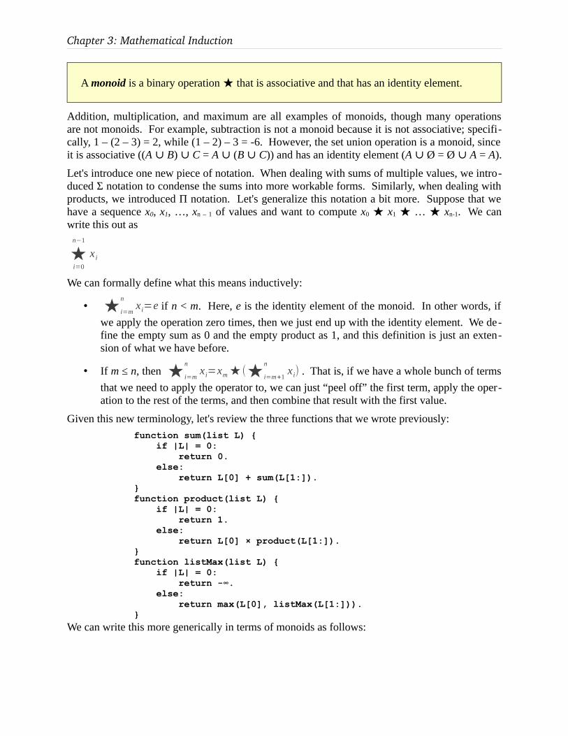
Chapter 3: Mathematical Induction

A monoid is a binary operation that is associative and that has an identity element.★

Addition, multiplication, and maximum are all examples of monoids, though many operations are not monoids. For example, subtraction is not a monoid because it is not associative; specifi-cally, 1 – (2 – 3) = 2, while (1 – 2) – 3 = -6. However, the set union operation is a monoid, since it is associative ((A ∪ B) ∪ C = A (∪ B ∪ C)) and has an identity element (A Ø = Ø∪ ∪ A = A).

Let's introduce one new piece of notation. When dealing with sums of multiple values, we intro-duced Σ notation to condense the sums into more workable forms. Similarly, when dealing with products, we introduced Π notation. Let's generalize this notation a bit more. Suppose that we have a sequence x0, x1, …, xn – 1 of values and want to compute x0 ★ x1 … ★ ★ xn-1. We can write this out as

★i=0

n−1

x i

We can formally define what this means inductively:

• ★i=m

nx i=e if n < m. Here, e is the identity element of the monoid. In other words, if

we apply the operation zero times, then we just end up with the identity element. We de-fine the empty sum as 0 and the empty product as 1, and this definition is just an exten-sion of what we have before.

• If m ≤ n, then ★i=m

nx i=xm★ (★i=m+1

nx i) . That is, if we have a whole bunch of terms

that we need to apply the operator to, we can just “peel off” the first term, apply the oper-ation to the rest of the terms, and then combine that result with the first value.

Given this new terminology, let's review the three functions that we wrote previously:

function sum(list L) { if |L| = 0: return 0. else: return L[0] + sum(L[1:]).}function product(list L) { if |L| = 0: return 1. else: return L[0] × product(L[1:]).}function listMax(list L) { if |L| = 0: return -∞. else: return max(L[0], listMax(L[1:])).}

We can write this more generically in terms of monoids as follows:

115 / 347

function fold(list L) { if |L| = 0: return e. else: return L[0] fold(L[1:]).★}

Here, as before, e is the identity element of the monoid. This function is sometimes called a fold, reduce, or accumulate function and is a staple in most functional programming languages. Assuming that is a monoid and that ★ e is its identity element, we can formally prove that this function is correct by generalizing our previous proofs:

Theorem: For any monoid and list ★ L, fold(L) = ★i=0

∣L∣−1

L [ i ]

Proof: By induction. Let be any monoid with identity element ★ e and define P(n) as fol-lows:

P(n) = “For any list L of length n, fold(L) = ★i=0

∣L∣−1L[ i ] .

We prove that P(n) is true for all n ∈ ℕ by induction. As our base case, we prove P(0),

that for any list L of length 0, that fold(L) = ★i=0

∣L∣−1L[ i ] . Note that fold(L) = e for any

empty list, and we have that★i=0

∣L∣−1L[ i ]=★i=0

−1L [ i ]=e . Thus fold(L) = ★i=0

∣L∣−1L[ i ]

as required.

For the inductive step, assume that P(n) holds for some n ∈ ℕ and that for all lists L of

length n, that fold(L) = ★i=0

∣L∣−1L[ i ] . We prove P(n + 1), that for all lists L of length

n + 1, that fold(L) = ★i=0

∣L∣−1L[ i ] . Consider any arbitrary list L of length n + 1. By defi-

nition, fold(L) in this case is L[0] ★ fold(L[1:]). For notational simplicity, let's let L' = L[1:]. The list L' has length n, since it consists of all elements of L except for the ele-

ment at position 0. By our inductive hypothesis, we have that fold(L') = ★i=0

∣L '∣−1L' [ i ] .

Now, we know that L' consists of all of the elements of L except for the first, so L'[i]

= L[i + 1] for all indices i. Therefore, we have fold(L') = ★i=0

∣L '∣−1L[ i+1 ] . We can then

adjust the indices to rewrite ★i=0

∣L '∣−1L[ i+1 ]=★ i=1

∣L'∣L[ i ] . Since |L'| = |L| - 1, we can

simplify this to ★i=1

∣L '∣L[ i ]=★i=1

∣L∣−1L[ i ] , so fold(L') =★i=1

∣L∣−1L[ i ] . This means that

fold(L) = L[0] ★ ★i=1

∣L∣−1

L [ i ] = ★i=0

∣L∣−1

L [ i ] .

Chapter 3: Mathematical Induction

Since our choice of L was arbitrary, this proves that for any list L of length n + 1, we have

that fold(L) = ★i=0

∣L∣−1

L [ i ] , completing the induction. ■

What we have just done is an excellent example of mathematics in action. We started with a col-lection of objects that shared some similar properties (in our case, recursive functions over list), then noticed that there was something similar connecting all of them. We then defined a new framework that captured all of our existing objects as special cases, then proved the result for the general result as a whole.

The beauty of what we've just done is that we immediately know that both of the following func-tions will work correctly:

function union(list L) { if |L| = 0: return Ø. else: return L[0] union(L[1:]).∪}function concatenateStrings(list L) { if |L| = 0: return "". else: return concat(L[0], concatenateStrings(L[1:])).}

If we want to prove correctness of these functions, we don't have to do a full inductive proof. In-stead, we can just prove that set union and string concatenation are monoids. I'll leave those proofs as exercises to the interested reader.

3.4 Variants on InductionWe have seen induction can be useful when proving properties that hold for all natural numbers. However, in many cases we are interested in proving properties of only a subset of the natural numbers – say, even numbers, powers of two, odd numbers, etc. In that case, it may be useful to use a variant of mathematical induction that captures the essential ideas of induction, but in a slightly different setting.

3.4.1 Starting Induction LaterLet's consider a simple question: what's bigger, n2 or 2n? If you have played around with these functions before, then your intuition probably tells you that 2n grows much, much more quickly than n2. For example, when n = 15, n2 = 225, while 2n = 32,768. However, if we plot the graphs of the two functions for small values, we see some interesting trends:

117 / 347

n n2 2n

0 0 1

1 1 2

2 4 4

3 9 8

4 16 16

5 25 32

6 36 64

Image from Google Graphs

As you can see, the two functions jockey for position. Initially, 2n is larger, but then n2 overtakes it. Once n = 5, 2n becomes larger. But given that these functions have fluctuated before, is it possible that n2 eventually catches up to and overtakes 2n?

It turns out that the answer is no. We can prove this in many ways, particularly differential cal-culus. However, we can also prove this result by induction. Namely, we will want to prove the following:

Theorem: For all n ∈ ℕ where n ≥ 5, n2 < 2n.

We won't concern ourselves with real numbers for now. Instead, we'll focus on natural numbers.

How exactly would we prove this? If we wanted to proceed by induction using the techniques we've seen so far, we would have to prove some claim about every natural number, not just the natural numbers greater than or equal to five. That said, it turns out that we can use our normal version of induction to prove this result. We will do this by being very clever with how we choose our property P(n). Specifically, what if we choose this property:

P(n) ≡ (n + 5)2 < 2(n + 5)

If we can prove that this claim is true for all n ∈ ℕ, then we will have proven the theorem. The reason for this is that if n ≥ 5, then we know that n – 5 must be a natural number. Consequently, the fact that P(n – 5) is true implies that ((n – 5) + 5)2 < 2((n – 5) + 5), which simplifies down to n2 < 2n, as required. Using this approach, our proof proceeds as follows:

Proof: By induction. Let P(n) ≡ (n + 5)2 < 2(n + 5). We will prove that P(n) holds for all n ∈ ℕ. From this, we can conclude that for any n ∈ ℕ with n ≥ 5 that (n + 5)2 < 2(n + 5). This holds because for any natural number n ≥ 5, we have that n – 5 ∈ . ℕ P(n – 5) then implies that n2 < 2n.

For our base case, we prove P(0), that 52 < 25. Since 52 = 25 and 25 = 32, this claim is true. For the inductive step, assume for some n that ∈ ℕ P(n) holds and (n + 5)2 < 2(n + 5). We will prove P(n + 1), that ((n + 5) + 1)2 < 2((n + 5) + 1). To see this, note that

Chapter 3: Mathematical Induction

((n + 5) + 1)2

= (n + 5)2 + 2(n + 5) + 1 (distributing)< 2n+5 + 2(n + 5) + 1 (by the inductive hypothesis)< 2n+5 + 2(n + 5) + 5 (since 1 < 5)≤ 2n+5 + 2(n + 5) + n + 5 (since 0 ≤ n)= 2n+5 + 3(n + 5) (collecting terms)< 2n+5 + 5(n + 5) (since 3 < 5)≤ 2n+5 + (n + 5)(n + 5) (since 0 ≤ n)= 2n+5 + (n + 5)2 (simplifying)< 2n+5 + 2n+5 (by the inductive hypothesis)= 2(2n+5) (simplifying)= 2((n + 5) + 1) (by powers of exponents)

Thus ((n + 5) + 1)2 < 2((n + 5) + 1), so P(n + 1) holds, completing the induction. ■

This proof is interesting for a few reasons. First, it shows that we can use induction to reason about properties of numbers larger than a certain size, though we have to be careful with how we phrase it. Second, it shows a style of proof that we have not seen before. To prove an inequality holds between two quantities, we can often expand out the inequality across multiple steps, at each point showing one smaller piece of the inequality. Since inequalities are transitive, the net result of these inequalities gives us the result that we want.

Let's try another example of a problem like this, this time using two other functions that grow quite rapidly: 2n and n!. n! is an extremely fast-growing function that dwarfs the comparatively well-behaved 2n. For example, for n = 10, 210 = 1,024, but n! = 3,628,800. However, for small values, we see the two functions vying for greatness:

n 2n n!

0 1 1

1 2 1

2 4 2

3 8 6

4 16 24

5 32 120From the looks of this table, it seems that as soon as n ≥ 4, n! ends up overtaking 2n. Does n! continue to dominate from this point forward? Or does 2n ever catch up?

Well, considering that we're about to prove the following theorem:

Theorem: For any n with ∈ ℕ n ≥ 4, 2n < n!.

119 / 347

it looks like n! is going to dominate from this point forward. The proof of this theorem is struc-turally quite similar to what we had before; the main changes are the fact that we're now starting from four, not five, and that our functions are different.

Proof: By induction. Let P(n) ≡ 2(n + 4) < (n + 4)!. We will prove that P(n) holds for all n ∈ ℕ. From this, we can conclude that for any n ∈ ℕ with n ≥ 4 that 2n < n!. This holds because for any natural number n ≥ 4, we have that n – 4 ∈ . ℕ P(n – 4) then implies that n2 < 2n.

For our base case, we prove P(0), that 24 < 4!. To see this, note that 24 = 16, while4! = 4 × 3 × 2 × 1 = 24. For the inductive step, assume that for some n ∈ that ℕ P(n) holds and 2(n + 4) < (n + 4)!. We will prove that P(n + 1) holds, that 2((n + 4) + 1) < ((n+4) + 1)!. To see this, note that

2((n + 4) + 1)

= 2(2(n + 4)) (using powers of exponents)< 2(n + 4)! (by the inductive hypothesis)< 5(n + 4)! (since 2 < 5)≤ (n + 5)(n + 4)! (since 0 ≤ n)= (n + 5)! (by definition of factorial)= ((n + 4) + 1)!

Thus 2((n + 4) + 1) < ((n + 4) + 1)!, so P(n + 1) holds, completing the induction. ■

The two proofs that we have just completed use induction, but are tricky to work with. In partic-ular, we want to prove a result about numbers greater than some specific threshold, but our proof instead works by showing a result for all numbers, using addition to shift everything over the ap-propriate number of steps.

Let's consider an alternative style of proof. Suppose that we want to repeat our previous proof (the one about n! and 2n). Can we just do the following:

• As our base case, prove that 24 < 4!.

• As our inductive step, assume that for some n ≥ 4, 2n < n! and prove that 2n + 1 < (n + 1)!.

In other words, this would be a normal inductive proof, except that we have shifted the base case up from 0 to 4, and now make an extra assumption during our inductive hypothesis that n ≥ 4. Otherwise, the proof proceeds as usual.

Of course, we're not even sure that it's mathematically legal to do this. Ignoring that (critical!) detail for now, though, let's see what the proof would look like were we allowed to write it. It turns out that the proof is much shorter than before and a lot easier to read:

Chapter 3: Mathematical Induction

Proof: By induction. Let P(n) ≡ 2n < n!. We will prove that P(n) holds for all n ∈ with ℕn ≥ 4 by induction.

For our base case, we prove P(4), that 24 < 4!. To see this, note that 24 = 16, while4! = 4 × 3 × 2 × 1 = 24.

For the inductive step, assume that for some n with ∈ ℕ n ≥ 4 that P(n) holds and 2n < n!. We will prove that P(n + 1) holds, meaning that 2n+1 < (n + 1)!. To see this, note that

2n + 1

= 2(2n) (by properties of exponents)< 2(n!) (by our inductive hypothesis)< (n + 1)(n!) (since 2 < 4 ≤ n < n + 1)= (n + 1)!

Thus 2n + 1 < (n + 1)!, so P(n + 1) holds, which completes the induction. ■

Wow! That's much cleaner, more succinct, and more clearly explains what's going on. The key step in this proof is the fact that we know that 2 < n + 1. This gives a good justification as to why 2n < n! once n gets to four – from that point forward, going from 2n to 2n + 1 doubles the pre-vious value, but going from n! to (n + 1)! increases the value by a factor of n + 1.

But how do we know that this is even a valid mathematical proof? The only reason that we know induction works is because it was specifically sanctioned as a mathematically valid form of reasoning. When we start making changes to induction, we can't necessarily guarantee that the resulting form of reasoning is sound. We will need to justify why the previous proof technique is legitimate before we start using it any further.

If you'll recall from Chapter Two, we proved that proof by contrapositive was legal by using proof by contradiction as a starting point. That is, we used one type of proof to show that some other type of proof was possible. We will now use normal mathematical induction to justify the above variant of induction, where we start off our induction from a value other than zero.

We will specifically prove the following theorem:

Theorem: Let P(n) be a property that applies to natural numbers and let k be a natural number. If the following are true:

P(k) is trueFor any n ∈ with ℕ n ≥ k, P(n) → P(n + 1)

Then for any n ∈ with ℕ n ≥ k, P(n) is true.

Compare this to the formal definition of the principle of mathematical induction from earlier in the chapter:

121 / 347

Let P(n) be a property that applies to natural numbers. If the following are true:

P(0) is trueFor any n ∈ ℕ, P(n) → P(n + 1)

Then for any n ∈ ℕ, P(n) is true.

Our goal will be to show that our initial definition of mathematical induction will allow us to prove that the above theorem is true.

In doing so it is critical to understand exactly what it is that we are trying to prove. Specifically, we want to show the following:

(Principle of Mathematical Induction) → (Induction Starting at k)

In order to do this, we will do the following. We want to show that if the following hold:

• P(k) is true

• For any n ∈ with ℕ n ≥ k, P(n) → P(n + 1)

Then we can conclude that

• For any n with ∈ ℕ n ≥ k, P(n) holds.

We will do this by means of a very clever trick. Suppose that we could define some new prop-erty Q(n) using P(n) as a building block. We will choose Q(n) such that it has two special prop-erties:

1. We can prove that Q(n) is true by induction on n.

2. If Q(n) is true for all natural numbers, then P(n) is true for all natural numbers greater than or equal to k.

These may seem totally arbitrary, but there is a good reason for them. For property (1), it's im-portant to realize that the property P(n) we're trying to reason about looks similar to the sort of property we would try to prove by induction. Unfortunately, since the base case doesn't start at 0, and since the inductive step makes some assumptions about the value of n, we can't immedi-ately use induction. If we could somehow adjust P(n) in a way so that it didn't have these two modifications, we could easily prove it by induction. Our choice of Q(n) will be a modified ver-sion of P(n) that does just that.

We want property (2) to hold so that we can find a connection between Q and P. If we don't have any restrictions on Q, then it's irrelevant whether or not we can prove it by induction. The trick will be to make it so that proving Q is true for all natural numbers shows that P is true for all natural numbers that are greater than or equal to k, which is precisely what we want to show.

The good news is that we already have seen two examples of how to build Q from P. The idea is actually quite simple – if we want to reason about numbers greater than or equal to k, we can just prove properties about natural numbers of the form n + k. Since every natural number greater than or equal to k must be k plus some smaller natural number, this means that we will have all of our cases covered. Specifically, we'll define

Chapter 3: Mathematical Induction

Q(n) ≡ P(n + k)

This is fairly abstract, so let's give some examples. Suppose we want to prove, as before, that n2 < 2n for n ≥ 5. In that case, we'd say that P(n) ≡ n2 < 2n. We then define Q(n) ≡ P(n + 5), which, if we expand it out, says that Q(n) ≡ (n + 5)2 < 2n + 5. If you look back at our first proof, this is exactly how we arrived at this result.

Given this setup, we can formally prove the theorem below.

Theorem: Let P(n) be a property that applies to natural numbers and let k be a natural number. If the following are true:

P(k) is trueFor any n ∈ with ℕ n ≥ k, P(n) → P(n + 1)

Then for any n ∈ with ℕ n ≥ k, P(n) is true.

Proof: Consider any property P(n) of the natural numbers for which the above is true. Now, define Q(n) ≡ P(n + k). This proof will work in two parts: first, we will prove, by in-duction, that Q(n) is true for all n . Next, we will show that this implies that ∈ ℕ P(n) is true for all n where ∈ ℕ n ≥ k.

First, we prove that Q(n) is true for all n by induction. As our base case, we prove ∈ ℕQ(0), meaning that P(k) holds. By our choice of P, we know that this is true. Thus Q(0) holds.

For the inductive step, assume that for some n that ∈ ℕ Q(n) is true, meaning that P(n + k) holds. We will prove that Q(n + 1) is true, meaning that P(n + k + 1) holds. Now, since n , we know that ∈ ℕ n ≥ 0. Consequently, we know that n + k ≥ k. Thus by the properties of P, we know that P(n + k) implies P(n + k + 1). Since Q(n + 1) ≡ P(n + k + 1), this proves that Q(n + 1) holds, completing the induction. Thus Q(n) is true for all natural numbers n.

Now, we use this result to prove that P(n) is true for all natural numbers n ≥ k. Consider any arbitrary natural number n ≥ k. Thus n – k ≥ 0, so n – k is a natural number. There-fore, Q(n – k) holds. Since (n – k) + k = n, this means that P(n) holds. Since our choice of n was arbitrary, this shows that P(n) is true for all natural numbers n ≥ k. ■

This proof is beautiful for several reasons. First, it combines proof by induction, which we've explored extensively in this chapter, with our previous style of proving that general claims are true – choose some arbitrary object, then show that the claim holds for that object. Second, it generalizes the two proofs that we did earlier in this section in a way that allows us to use this new, much more powerful form of induction. From this point forward, we can start off our in-ductions anywhere in the natural numbers, using the proof we have just done to conclude that we have proven a result about all natural numbers greater than or equal to some starting value.

123 / 347

3.4.2 Fibonacci InductionThe Fibonacci sequence is a famous mathematical sequence that appears in a surprising number of places. The sequence is defined as follows: the first two terms are 0 and 1, and each succes-sive term is the sum of the two previous terms. For example, the first several terms of the Fi-bonacci sequence are

0, 1, 1, 2, 3, 5, 8, 13, 21, 34, 55, 89, …

Formally speaking, we can define the Fibonacci sequence using this beautiful inductive defini-tion:

• F0 = 0

• F1 = 1

• Fn + 2 = Fn + Fn + 1

From our perspective, the Fibonacci sequence is interesting in that it is clearly defined induc-tively (every term is defined by the two terms that precede it), but we cannot immediately use our principle of induction to prove its properties. Using the forms of induction we've seen so far, we can use knowledge about n to prove properties about n + 1. For the Fibonacci sequence, we need to use information about n and n + 1 to prove properties about n + 2. This slight difference – the fact that we rely on the last two terms to reason about the next term – complicates proofs about Fibonacci numbers.

In order to prove properties about the Fibonacci sequence or numbers related to them, we will need a new type of induction specifically suited to working with the Fibonacci sequence. Specif-ically, we'll try to construct our induction so that it mirrors the shape of the Fibonacci numbers. If we want to prove that some property P(n) holds for the nth Fibonacci number, it would make sense to try to prove the following:

• P(n) holds for the zeroth and first Fibonacci numbers.

• If P(n) holds for the nth and (n+1)st Fibonacci numbers, then it holds for the (n+2)nd Fi-bonacci number.

From this, it should seem reasonably intuitive that we could claim that P(n) holds for all Fi-bonacci numbers. We could see this because

• P(0) and P(1) hold.

• Because P(0) and P(1) hold, P(2) holds.

• Because P(1) and P(2) hold, P(3) holds.

• Because P(2) and P(3) holds, P(4) holds.

• …

As with our previous result that we can fire off induction from any starting point, we will need to formally prove that this form of induction (which we'll dub Fibonacci induction) actually works correctly. Our goal will be to prove this theorem:

Chapter 3: Mathematical Induction

Theorem: Let P(n) be a property that applies to natural numbers. If the following are true:

P(0) is true.P(1) is true.For any n ∈ ℕ, P(n) and P(n + 1) → P(n + 2)

Then for any n ∈ ℕ, P(n) is true.

Again, our starting point is that we know the principle of mathematical induction to be true. We will somehow have to use this as a building block in order to show that the above theorem – which gives rise to its own style of proof – is indeed correct.

Our proof will be similar to the one we did last time. The objective will be to define some new property Q(n) in terms of P(n) such that

• Q(n) can be proven true for all n using the principle of mathematical induction, and∈ ℕ

• If Q(n) is true for all n , then ∈ ℕ P(n) is true for all n .∈ ℕ

The trick will be choosing an appropriate Q(n). To do so, let's review why this style of proof works in the first place. If you look at the informal logic we used on the previous page, you'll note that we started with P(0) and P(1) and used this to derive P(2). Then, from P(1) and P(2), we derived P(3). From P(2) and P(3), we derived P(4). If you'll notice, each step in this proof works by assuming that P(n) is true for the last two choices of n, then using that to prove that P(n) holds for the next choice of n. This suggests that perhaps we'll want our choice of Q(n) to encode the idea that two adjacent values of P(n) still holds. For example, what if we try choos-ing Q(n) as

Q(n) ≡ P(n) and P(n + 1)

Could we use this to prove that Q(n) is true for all n by induction? Well, we'd first have to∈ ℕ prove that Q(0) holds, meaning that P(0) and P(1) are true. Fortunately, we already know that – this is one of the two properties we know of P(n). Great!

So could we prove the inductive step? Our goal here would be to show that if Q(n) holds (mean-ing that P(n) and P(n + 1) are true), then Q(n + 1) holds (meaning that P(n + 1) and P(n + 2) are true). Half of this is easy – if we're already assuming that P(n + 1) is true to begin with, then we don't need to prove P(n + 1) is true again. However, we do need to prove that P(n + 2) is true. But we've chosen P(n) such that P(n) and P(n + 1) collectively imply P(n + 2). This means that if we know that P(n) and P(n + 1) are true, we can easily get that P(n + 1) and P(n + 2) are true. In other words, if Q(n) is true, then Q(n + 1) must be true as well. Excellent!

We can formalize this intuition below in the following proof:

125 / 347

Theorem: Let P(n) be a property that applies to natural numbers. If the following are true:

P(0) is true.P(1) is true.For any n ∈ ℕ, P(n) and P(n + 1) → P(n + 2)

Then for any n ∈ ℕ, P(n) is true.

Proof: Let P(n) be an arbitrary property with the above set of traits. Let Q(n) ≡ “P(n) and P(n + 1).” We will prove that Q(n) is true for all n by induction on ∈ ℕ n. Once we have proven this, we will show that if Q(n) is true for all n , it must be the case that ∈ ℕ P(n) is true for all n .∈ ℕ

To see that Q(n) is true for all n , we proceed by induction. First, we prove that ∈ ℕ Q(0) is true; namely, that P(0) and P(1) are true. By our choice of P(n), we know these proper-ties are true, so Q(0) holds.

For the inductive step, assume that for some n that ∈ ℕ Q(n) is true, meaning that P(n) and P(n + 1) are true. We will prove Q(n + 1) is true, meaning that P(n + 1) and P(n + 2) are true. By our inductive hypothesis, we already know that P(n + 1) is true, so we just need to show that P(n + 2) is true as well. By our choice of P(n), we know that since P(n) and P(n + 1) are true, we have that P(n + 2) is true as well. Thus we have that P(n + 1) and P(n + 2) hold, so Q(n + 1) holds as well, completing the induction.

Finally, we need to show that because Q(n) is true for all n , we know that ∈ ℕ P(n) is true for all n . To see this, note that for any ∈ ℕ n , we know that ∈ ℕ Q(n) is true, so P(n) and P(n + 1) are true. Ignoring the extra detail that P(n + 1) is true, we now have that P(n) is true as well. Since our choice of n was arbitrary, this proves that P(n) holds for alln . ■∈ ℕ

Cool! We now have a proof technique we can use to reason about the Fibonacci numbers. Let's not just leave this sitting on the shelf; instead, let's go and use it to prove some interesting prop-erties about Fibonacci numbers and related problems!

3.4.2.1 Climbing Down Stairs

Let's start off by tackling a simple problem that has a rather surprising solution. Let's suppose that you're standing at the top of a staircase, like this one:

Chapter 3: Mathematical Induction

You want to get down to the base of the staircase. In doing so, you can walk down using steps of size one or steps of size two (but not any more – you don't want to come tumbling down the stairs!) For example, here are two different paths you could take down the above staircase:

Now, the question – how many paths down a staircase of size n can you take?

If you take any reasonable-sized staircase, you'll find that there can be a lot of paths down. For example, if you have the above staircase, there are eight different paths down:

The number of paths just keeps getting bigger and bigger as the staircase gets higher and higher. Can we find a nice expression that will tell us exactly how many paths down the stairs there are?

When faced with a problem like this, one reasonable approach would be to list off all the paths that we can find, then check whether or not we can find a pattern in how they're constructed. For the staircase with five stairs, we can write out those paths as a sequence of 1s and 2s,

127 / 347

• 1 1 1 1 1

• 1 1 1 2

• 1 1 2 1

• 1 2 1 1

• 2 1 1 1

• 2 2 1

• 2 1 2

• 1 2 2

There are a lot of patterns we can exploit here. Notice, for example, that the first path (1 1 1 1 1) is just all 1s. The next four paths consist of all possible permutations of three 1s and one 2. The last three paths consist of all possible permutations of two 2s and a 1. If we counted up how many ways there were to set up these sorts of permutations, we could arrive at our answer.

While the above approach works, it's a bit complicated and we might have better luck looking for other patterns. What if we sorted the above sequences lexicographically (the way that you would order words in a dictionary?) In that case, we get the following sequence of paths:

• 1 1 1 1 1

• 1 1 1 2

• 1 1 2 1

• 1 2 1 1

• 1 2 2

• 2 1 1 1

• 2 1 2

• 2 2 1

Now, we can start to see a different structure emerging. Notice that for each of the paths that start with a 1, the structure of the path is a 1 followed by some path from the fourth step all the way back down to the bottom of the stairs. Each of the paths that start with a 2 have the form of a path starting with a step of size 2, followed by a path from the third stair all the way down. In -tuitively, this makes sense – to get down, you either take a step down one stair and then some path back down from there, or you take a step down two stairs and then some path back down from there.

This observation can actually be used to develop a way of computing the number of paths down the stairs. Assuming that we start out sufficiently “high enough” on the stairs that there's room to take steps of size one and size two, then the total number of paths back down the stairs must be equal to the number of paths that start with a step of size one, plus the number of paths that start with a step of size two. Since each path starting with a step of size one initially takes us from stair n to stair n – 1, and each path starting with a step of size two initially takes us from stair n to stair n – 2, this means that the number of paths down the stairs from stair n is given by the num-ber of paths down from stair n – 1, plus the number of paths down from stair n – 2.

What this says is that if we're sufficiently high up on the stairs that we can take steps of size 1 and size 2, we can determine the number of paths down based on the number of paths from the stairs one and two steps below us. But what if we're very near the bottom of the staircase and can't do this? Well, the only way that we couldn't take a step of size 1 and a step of size 2 would be if we are standing on stair 1, or we are at the bottom of the staircase. If we are at stair 1, then there is exactly one path down – just take a step of size one down to the bottom.

But what if we are at the base of the staircase? How many paths are there now? This is a subtle but important point. Initially, we might say that there are zero paths, since you can't take any steps here. But this would be mathematically misleading. If there are indeed zero paths once you're standing at the base of the staircase, then it would mean that there is no way to get to the bottom of the staircase once you're already there. This seems suspicious. Ask yourself the fol-

Chapter 3: Mathematical Induction

lowing question – can you get to where you are sitting right now from your current location? You'd probably think “yes – I'm already there!” In fact, for this very reason, it would be inappro-priate to say that there are zero paths down the stairs from the bottom of the staircase. Rather, there is exactly one path, namely, not moving at all.

The thing to remember here is that there is a difference between “there are no paths” and “the only path is the empty path.” When dealing with problems like these, it is critical to remember to maintain a distinction between “unsolvable” and “trivially solvable.” Many problems have silly solutions for small cases, but those solutions are still indeed solutions!

Okay – at this point, we have a nice intuition for the number of paths down:

• There is exactly one path down from a staircase of height 0 or height 1.

• For staircases with two or more steps, the number of paths down is the sum of the number of paths down for a staircase of one fewer step plus the number of paths down for a stair-case of two fewer steps.

Let's try to make this a bit more formal. Let's define a sequence Sn representing the number of paths down from a staircase of height n. Translating the above intuition into something a bit more mathematically rigorous, we get that

• S0 = S1 = 1.

• Sn+2 = Sn + Sn+1.

Now that we this recurrence, we can start evaluating a few terms from it to see if we can recog-nize it from somewhere. If we start expanding this out, we get the sequence

1, 1, 2, 3, 5, 8, 13, 21, …

This should look very familiar – it's the Fibonacci sequence, shifted over by one term! Now that is indeed surprising. The problem we described – walking down a staircase – superficially bears no resemblance at all to the Fibonacci sequence. This isn't particularly unusual, though, since the Fibonacci sequence tends to arise in all sorts of surprising contexts.

Are we satisfied that the number of paths down from a staircase of height n is the (n + 1)st Fi-bonacci number? We've arrived at our result intuitively, but we haven't actually proven anything yet. To wrap up this problem, and to put our new Fibonacci induction proof technique to use, let's formally establish the above result:

Theorem: On a staircase of n stairs, there are Fn+1 paths from the top of the staircase down to the bottom using step sizes of 1 and 2.

Proof: By induction. Let P(n) be “On a staircase of n stairs, there are Fn+1 paths from the top of the staircase down to the bottom using step sizes of 1 and 2.” We will prove that P(n) is true for all n .∈ ℕ

129 / 347

As our base cases, we prove that P(0) and P(1) are true; that is, there are F1 and F2 paths down staircases of heights 0 and 1, respectively. In the case of a staircase of height 0, there is exactly one path down the staircase, namely, the path of no steps. Since F1 = 1, the claim holds for P(0). For a staircase of height 1, there is exactly one path down, which is to take a step of size one. Since F2 = 1, the claim holds for P(1).

For the inductive step, assume that for some n , that ∈ ℕ P(n) and P(n + 1) hold and that the number of paths down staircases of heights n and n + 1 using only step sizes of 1 and 2 is Fn+1 and Fn+2, respectively. We want to prove P(n + 2), namely that the number of paths down a staircase of height n + 2 using steps of size 1 and 2 is Fn+3. To see this, consider any path down such a staircase. This path must either begin with a step of size 1, in which case the path is formed by taking a path down a staircase of size n + 1 and extending it by one step, or it must begin with a step of size 2, in which case the path is formed by taking a path down a staircase of size n and extending it by one step. Consequently, the number of paths down the staircase of height n + 2 is given by the number of paths down staircases of heights n and n + 1. By our inductive hypothesis, these numbers are Fn+1 and Fn+2. Conse-quently, the number of paths down is Fn+1 + Fn+2 = Fn+3, as required. Thus P(n + 2) holds, completing the induction. ■

3.4.2.2 Computing Fibonacci Numbers

The Fibonacci numbers are often introduced as a simple function that can be computed easily with recursion. Typically, the recursive function is presented as follows:

int fib(int n) {   if (n == 0) return 0;   if (n == 1) return 1;   return fib(n – 1) + fib(n – 2);}

We can prove that this function is correct by induction on n:

Theorem: For any n , ∈ ℕ fib(n) = Fn.

Proof: By induction on n. Let P(n) ≡ “fib(n) = Fn.” We prove that P(n) is true for all n ∈ by induction.ℕ

For our base case, we prove P(0) and P(1); namely, that fib(0) = F0 and that fib(1) = F1. To see this, note that by construction, fib(0) = 0 = F0 and fib(1) = 1 = F1. Thus P(0) and P(1) hold.

Chapter 3: Mathematical Induction

For our inductive step, assume that for some n that P(n) and P(n + 1) hold and that fib(n)= Fn and fib(n + 1) = Fn+1. We prove P(n + 2), that fib(n + 2) = Fn+2. To see this, note that since n + 2 ≥ 2, n + 2 ≠ 0 and n + 2 ≠ 1. Consequently, fib(n + 2) = fib(n) + fib(n + 1). By our inductive hypothesis, this means that fib(n + 2) = Fn + Fn+1 = Fn+2, as required. Thus P(n + 2) holds, completing the induction. ■

Great – so we now have a function for computing Fibonacci numbers! But how efficient is it? To measure the complexity of this fib function, we should count some quantity that measure the total amount of work being done. One measure of complexity which might be good here is how many total function calls end up being required. Since each function does at most some fixed amount of work (namely, declaring variables, checking a fixed number of if statements, making a fixed number of recursive calls, and extra logic like setting up and tearing down the stack frame), we can claim that the total work done is proportional to the number of function calls made.

To determine how many function calls are made, we can start off by drawing out a recursion tree, a diagram of which function calls invoke which other function calls. Here are the recursion trees for n = 0, 1, 2, 3, and 4:

F0

F1

F2

F0

F1

F1

F2

F0

F1

F3

F2

F0

F1

F1

F2

F0

F1

F3

F4

If we count up the number of nodes in these trees, we get 1, 1, 3, 5, 9, …, which doesn't seem to be any sequence that we know so far. Perhaps we could investigate the structure of this sequence in more depth to try to arrive at a nice formula for it.

To start things off, let's see if we can write out some nice recurrence that describes the terms in the series. Looking over our recursive function, we can note the following:

• If n = 0 or n = 1, exactly one function call is necessary.

• Otherwise, we need one function call for the initial call, plus a number of calls necessary to evaluate fib(n – 1), plus a number of calls necessary to evaluate fib(n – 2).

Let's denote by Cn the number of function calls required to compute fib(n). Translating the above definition, we end up getting that Cn is defined as follows:

• C0 = C1 = 1.

• Cn+2 = Cn + Cn+1 + 1.

This is similar to the Fibonacci series, but it's not quite the same. Specifically, the Fibonacci se-quence starts off with the first two terms 0, 1, and doesn't have the +1 term in the recurrence step. In case you're curious, the first few terms of this series are

1, 1, 3, 5, 9, 15, 25, 41, 67, 109, 177, …

131 / 347

The question now becomes how we can try to get a value for Cn, preferably in terms of the Fi-bonacci sequence Fn. There are many different approaches we can take here, and in this section we'll see two approaches, each based on a different techniques.

The first technique that we can use is based on the following idea. The above recurrence looks a lot like the normal Fibonacci sequence, but with a few extra 1s thrown into the mix. Could we somehow separate out Cn into two terms – one term based on the Fibonacci sequence, plus one extra term based on the extra +1's?

To apply this technique, we will do the following. First, let's try to identify how much of this re-currence we can attribute to the Fibonacci sequence. One observation we can have is that since the first two terms of the sequence are 1s and each successive term depends (partially) on the sum of the previous two terms, we could consider thinking of this sequence as the Fibonacci se-quence shifted over one step (as in the staircase problem), plus some extra terms. Specifically, let's see if we can write

Cn = Fn+1 + En

Where En is some “extra” term thrown into the mix to account for the extra 1s that we keep accu-mulating at each step. In other words, we can write

En = Cn – Fn+1

If we can now find some value for En, then we will end up being able to compute a value for Cn

in terms of the (n+1)st Fibonacci number Fn+1 and the sequence Cn. We still don't know how to compute En yet, but we've at least stripped away some of the complexity of our original problem.

In order to learn what En is, we should probably try writing out some values for Cn – Fn+1. Below are the values for this sequence:

Cn 1 1 3 5 9 15 25 41 67

Fn+1 1 1 2 3 5 8 13 21 34

En 0 0 1 2 4 7 12 20 33

Now this is interesting. If you'll notice, the value of En, the extra number of 1s added into the se-quence, is always exactly one less than Fn+1. In other words it appears that, En = Fn+1 – 1. Given that Cn = Fn+1 + En, this would mean that Cn = Fn+1 + (Fn+1 – 1) = 2Fn+1 – 1.

We haven't actually proven this yet, nor do we have much of an intuition for why this would be true. If we are purely interested in coming up with an answer to the question “how many func-tion calls are made?,” however, we don't actually need to know why. We can use a quick induc-tive proof to show that we have to be correct. (Don't worry – we'll definitely come back to why this is true in a minute).

Theorem: The number of function calls required to compute fib(n) is 2Fn+1 – 1.

Chapter 3: Mathematical Induction

Proof: By induction. Let P(n) be “fib(n) makes 2Fn+1 – 1 function calls.” We will prove that P(n) is true for all n by induction.∈ ℕ

For our base cases, we prove P(0) and P(1); namely, that fib(0) makes 2F1 – 1 function calls and that fib(1) makes 2F2 – 1 function calls. In the case of both fib(0) and fib(1), ex-actly one function call is made, specifically the initial calls to fib. Since F1 = F2 = 1 and 2F1 – 1 = 2 – 1 = 1, this means that fib(0) makes 2F1 – 1 calls and fib(1) makes 2F2 – 1 calls, as required. Thus P(0) and P(1) hold.

For the inductive step, assume that for some n that P(n) and P(n + 1) hold, meaning that fib(n) makes 2Fn+1 – 1 calls and fib(n + 1) makes 2Fn+2 – 1 calls. We will prove P(n + 2), that fib(n + 2) makes 2Fn+3 – 1 calls. To see this, consider the number of calls required to evaluate fib(n + 2). The number of calls required is 1 for the initial call to fib(n + 2), plus the number of calls required to evaluate fib(n) and fib(n + 1). By the inductive hypothesis, these values are 2Fn+1 – 1 and 2Fn+2 – 1, respectively. Thus the total number of calls is

1 + 2Fn+1 – 1 + 2Fn+2 – 1= 2Fn+1 + 2Fn+2 + 1 – 1 – 1= 2(Fn+1 + Fn+2) – 1= 2Fn+3 – 1

Thus 2Fn+3 – 1 calls are required to evaluate fib(n + 2), so P(n + 2) holds, completing the induction. ■

The numbers 1, 1, 3, 5, 9, 15, 25, … are important in computer science and are called the Leonardo numbers. We denote the nth Leonardo number by Ln. The previous proof shows that Ln = 2Fn+1 – 1.

The above proof tells us that we at least have the right answer – the number of recursive calls is indeed 2Fn+1 – 1. However, it doesn't give us any insight whatsoever about where this number comes from. How on earth did we arrive at this figure?

Let's revisit the intuition that led us here. We separated Cn into two terms – the (n + 1)st Fi-bonacci number Fn+1, plus some “extra” term En. Let's investigate exactly where each term comes from.

The key insight we need to have here is exactly how fib(n) computes Fn. I've reprinted this func-tion below for simplicity:

int fib(int n) {   if (n == 0) return 0;   if (n == 1) return 1;   return fib(n – 1) + fib(n – 2);}

Notice that the fib function works in one of two ways. First, for its base cases, it directly returns a value. For the recursive step, fib computes Fn by computing Fn-2 and Fn-1 and adding those val-ues together. But those values originally came from adding up even smaller Fibonacci numbers, which in turn came from adding up even smaller Fibonacci numbers, etc. Ultimately, the value

133 / 347

returned by this function is derived by adding up the 0s and 1s returned in the base cases the ap-propriate number of times. You can see this below by reexamining the recursion trees for com-puting fib(n):

F0

F1

F2

F0

F1

F1

F2

F0

F1

F3

F2

F0

F1

F1

F2

F0

F1

F3

F4

If we replace each function call with the value it returns, we get the following:

0 1 1

0 1 1 1

0 1

2

1

0 1 1 1

0 1

2

3

Each of the numbers is the sum of the numbers below it, which in turn are the sum of the num-bers below them, until the recursion bottoms out into the base cases.

So now we can ask: how many of the function calls are base cases (values that actually produce the values), and how many of the function calls are recursive cases that just combine together previously-produced values?

Below are the above recursion trees, with all of the recursive function calls highlighted in yellow, all of the base cases highlighted in magenta:

0 1 1

0 1 1 1

0 1

2

1

0 1 1 1

0 1

2

3

So how many of the function calls in each recursion tree are of each type? Notice that the num-ber of magenta circles in each of the recursion trees is given by the following sequence:

1, 1, 2, 3, 5, 8, 13, …

This is the Fibonacci sequence shifted by one, which explains why we're getting some term that depends on Fn+1. Now, how many yellow circles are there? Notice that it's always equal to the number of magenta circles minus one. The reason for this is structural. Let's begin with any col-lection of Fn+1 magenta nodes representing the base cases; for example, like this:

Chapter 3: Mathematical Induction

0 1 1

0 1

Initially, all of these function calls are disconnected – there is nothing combining them together. In order to link them together into a recursion tree, we will need to link them together by the other function calls that called them. For example, we might add in this call:

0 1 1 1

0 1

Now, let's count how many different, disconnected “pieces” of the tree remain. Initially, we had five different function calls, each of which were isolated. Adding in this yellow function call re-duces this down to four isolated pieces. In other words, adding in a yellow node decreased the number of disconnected pieces by one.

Every time we introduce one of the yellow internal nodes to connect together two trees that are previously disconnected, we decrease the number of disconnected trees by one. We ultimately need to end up with a single recursion tree, which means that we need to pairwise merge all Fn+1

disconnected trees together into a single tree. This means that we will need to do Fn+1 – 1 merges, each of which introduces a yellow node. Consequently, the total number of nodes will be Fn+1 + (Fn+1 – 1) = 2Fn+1 – 1. This gives a completely different but equally valid argument for why this must be the correct number of nodes in the tree.

3.5 Strong InductionThe flavors of induction we've seen so far – normal induction, induction starting at k, and Fi-bonacci induction – have enabled us to prove a variety of useful results. We will now turn to an even more powerful form of induction called strong induction that has numerous applications within computer science, from the analysis of algorithms to the understanding of the structure of numbers themselves.

To motivate strong induction, let's take a minute to think about how normal induction works. In a proof by induction, we first show that some property holds for 0 (or some other starting num-ber, as you saw before). We then conclude “since it's true for 0, it's true for 1,” then conclude “since it's true for 1, it's true for 2,” then conclude “since it's true for 2, it's true for 3,” etc. No-tice that at each step in the induction, we only use the most recent result that we have proven in order to get to the next result. That is, to prove that the result is true for three, we only use the fact that the result is true for two, and not that it's true for zero or one. Similarly, if we wanted to prove that the result holds for a large number (say, 137), our proof would only rely on the fact that the result was true for 136.

In a sense, it seems like we're handicapping ourselves. Why must we only rely on the most re-cent result that we have proven? Why can't we use the entire set of all the results we've proven so far in order to establish the next result?

This is the intuition behind a powerful type of induction called strong induction:

135 / 347

Theorem (strong induction): Let P(n) be a property that applies to natural numbers. If the following are true:

P(0) is true.For any n , if ∈ ℕ P(0), P(1), …, P(n) are true, then P(n + 1) is true.

Then for any n ∈ ℕ, P(n) is true.

Compare this to the normal principle of mathematical induction. In a regular induction, we would assume that P(n) is true, then use it to show that P(n + 1) is true. In strong induction, we assume that all of P(0), P(1), …, and P(n) are true, then use this to show that P(n + 1) is true.

To give a sort of intuition for strong induction, let's work through a simple example that shows how to use this style of proof technique. Suppose that you have a chocolate bar consisting of n + 1 smaller squares of chocolate, all in a line. For example, the candy bar might look like this:

M A T H !

You want to break this chocolate bar apart into n + 1 squares. How many breaks do you have to make in the chocolate bar in order to completely break it down?

Let's try some examples. If you have a chocolate bar with 6 pieces, then you'll need to make five total breaks – one in-between each of the pieces of chocolate. If the chocolate bar has 137 pieces, you'd need 136 breaks. In general, it seems like you need to break the chocolate bar n times if it has n + 1 squares, since there are n separators.

This result might not seem all that impressive, but if we actually want to prove that this is opti -mal, we will need to be a bit more careful. Surely we can break the candy bar apart with n breaks, but can we do it in fewer than n breaks? The answer is no, and to prove this we will show the following result:

Theorem: Breaking a linear candy bar with n + 1 pieces down into its individual pieces re-quires at least n breaks.

How exactly can we show this? Well, we would somehow need to show that no matter how you try to break the candy bar apart, you always have to make at least n breaks. To do this, we can try the following line of reasoning – consider any possible way to break apart the candy bar, then show that no matter how it's done, it always uses at least n breaks.

So what is it like to break apart a candy bar this way? If you think about it, any way that we break apart the candy bar must start with some initial break, which will split the candy bar into two smaller pieces. From there, we can start breaking those smaller pieces down even further, and those smaller pieces down even further, etc. For example, here is one way of breaking down a candy bar with six pieces:

Chapter 3: Mathematical Induction

C A N D Y !

C A N D Y !

C A N D Y !

C A N D Y !

C A N D Y !

Now for the key insight: notice that as soon as we break the chocolate bar with the first break, we are left with two smaller chocolate bars. In order to break the overall chocolate bar down into in-dividual squares, we will need to break those smaller pieces down into their individual parts. Consequently, we can think of any approach for breaking the chocolate bar down as follows:

• Make some initial break in the chocolate bar.

• Break the remaining pieces of chocolate down into their constituent pieces.

At some point this process has to stop, and indeed we can see that once we get down to a choco -late bar of size one, there is no longer any work to do.

Using this insight, we can prove by strong induction that the total number of breaks required is at least n. To do so, we'll initially prove the base case – that a chocolate bar with one piece requires no breaks – and from there will show that no matter how you break the chocolate bar into pieces, the total number of breaks required to subdivide the remaining pieces, plus the initial break, is al-ways at least n if the chocolate bar has n + 1 pieces in it.

Here is the proof; we'll discuss it in some depth immediately afterwards:

Proof: By strong induction. Let P(n) be “breaking a linear chocolate bar with n + 1 pieces down into its constituent pieces requires at least n breaks.” We will prove P(n) holds for all n by strong induction on ∈ ℕ n.

For our base case, we prove P(0), that any way of breaking a chocolate bar consisting of a single square into its constituent pieces takes at least zero breaks. This is true, since if there is just one square, it is already broken down as far is it can be, which requires no breaks.

137 / 347

For our inductive step, assume that for some n , that for any ∈ ℕ n' with ∈ ℕ n' ≤ n, that P(n') holds and breaking a candy bar with n' + 1 pieces into its squares takes at least n' breaks. We will prove P(n + 1), that breaking a candy bar with n + 2 pieces requires at least n + 1 breaks. To see this, note that any way that we can break apart this candy bar will consist of an initial break that will split the candy bar into two pieces, followed by subsequent breaks of those smaller candy bars. Suppose that we break the candy bar such that there are k + 1 squares left in one smaller piece and (n + 2) – (k + 1) = (n – k) + 1 pieces in the second piece. Here, k + 1 must be no greater than n + 1, since if it were, we would have n + 2 squares in one smaller piece and 0 in the other, meaning that we didn't actually break anything. This means that k + 1 ≤ n + 1, so k ≤ n. Thus by our strong in-ductive hypothesis, we know that it takes at least k breaks to split the piece of size k + 1 into its constituent pieces. Similarly, since k ≥ 0, we know that n – k ≤ n, so by our induc-tive hypothesis it takes at least n – k breaks to break the piece of size (n – k) + 1 into its constituent pieces. This means that for any initial break, the total number of breaks re-quired is at least (n – k) + k + 1 = n + 1, as required. Thus P(n + 1) holds, completing the induction. ■

Let's dissect this proof and see exactly how it works. First, notice that we began the proof by an-nouncing that we were going to use strong induction. Just as you should start a proof by induc-tion, contradiction, or contrapositive by announcing how your proof will proceed, you should start proofs by strong induction with an explicit indication that this is what you are doing. It will make your proof much easier to read.

Notice that in the above proof, the proof of the base case proceeded as usual. We state what P(0) is, then go prove it. However, the inductive step starts out noticeably differently from in our pre-vious proofs by induction. Notice that it began as follows:

For our inductive step, assume that for some n , that for any ∈ ℕ n' with ∈ ℕ n' ≤ n, that P(n') holds and breaking a candy bar with n' + 1 pieces into its squares takes at least n' breaks.

Here, we are not just assuming that P(n) holds for some choice of n. Instead, we are assuming that we already know that P(0), P(1), P(2), … P(n) are true. Rather than writing this out long-hand, we use a more compact notation and say that P(n') is true for any n' ≤ n. Most proofs by strong induction will proceed this way, and it is a good idea to make sure you understand why this notation with n' is equivalent to listing off all the smaller choices of n.

From there, the proof proceeds more or less as usual – we explain why we can reason about the initial break, and then introduce the variable k to reason about how many squares are in each side. However, there is one key step to pay attention to. In the body of the inductive step, we in-voke the inductive hypothesis twice, once for each piece of the chocolate bar. Notice how we do it:

Chapter 3: Mathematical Induction

Here, k + 1 must be no greater than n + 1, since if it were, we would have n + 2 squares in one smaller piece and 0 in the other, meaning that we didn't actually break anything. This means that k + 1 ≤ n + 1, so k ≤ n. Thus by our strong inductive hypothesis, we know that it takes at least k breaks to split the piece of size k + 1 into its constituent pieces. Similarly, since k ≥ 0, we know that n – k ≤ n, so by our inductive hypothesis it takes at least n – k breaks to break the piece of size (n – k) + 1 into its constituent pieces.

Before we claim that we can use the inductive hypothesis on the smaller pieces, we first verify that the size of each smaller piece is indeed no greater than n. It is critical that you do some-thing like this in any proof by strong induction. The inductive hypothesis only applies to natural numbers that are less than or equal to n, and if you want to apply the inductive hypothesis to something of size n', you need to first demonstrate that n' ≤ n.

3.5.1 The Unstacking GameLet's continue our exploration of strong induction with a simple game with a surprising strategy. This game, called the unstacking game, works as follows.* At the start of the game, you are pre-sented a stack of n + 1 identical blocks. Your goal is to unstack all the boxes so that you are left with n + 1 stacks consisting of one block each. To do so, you are allowed to take a stack of at least one block, then “unstack” that block by splitting it into two stacks, where each stack has at least one block in it. For example, if you are playing this game with seven blocks, the game might start out like this:

As your first move, you might split this tower into two stacks, one with two blocks and one with five blocks, as shown here:

* I first heard this problem from Prof. Dieter van Melkebeek of the University of Wisconsin.

139 / 347

Your next move might be to split the stack of five blocks into two stacks, one with four blocks and one with one block, as seen here:

If you'll notice, so far this game is identically the same as the breaking chocolate problem – we have a linear stack of blocks, and keep breaking that stack into smaller and smaller pieces. What differentiates this game from the chocolate bar problem is that you are awarded a different num-ber of points based on how you break the stack into two pieces. In particular, with each move, you earn a number of points equal to the product of the number of blocks in the each of the smaller stacks that you create. For example, in the first move, above, you would earn ten points (5 × 2), and in the second move you would earn four points (4 × 1).

Now, for the key question: what strategy should you use to maximize the number of points that you earn?

When confronted with a problem like this one, sometimes the best option is to try out a bunch of different ideas and see how they pan out. Let's consider, for example, a stack of eight blocks. If we are trying to maximize our score, then we might consider a few different strategies. Since our score depends on the product of the sizes of the splits we make, one option might be, at each point, to split the largest tower we have in half. This maximizes the score we get at each step, though it rapidly decreases the size of the remaining towers. Another option might be to always just peel off one block from the tower at a time. This would mean that each turn individually doesn't give us that many points back, but would mean that the rate at which the tower shrinks is minimized, thus giving us more points for a longer period of time.

Let's try these strategies out! If we adopt the first strategy and keep splitting the largest tower cleanly in half, then we get the following game:

Chapter 3: Mathematical Induction

This gives us a net of 28 points. If we adopt the second strategy, though, we get this game:

4 × 4 = 16 2 × 2 = 4 2 × 2 = 4 1 × 1 = 1

1 × 1 = 1 1 × 1 = 1

1 × 1 = 1

16 + 4 + 4 + 1 + 1 + 1 + 1 = 28

1 × 7 = 7 1 × 6 = 6 1 × 5 = 5 1 × 4 = 4

1 × 3 = 3 1 × 2 = 2

1 × 1 = 1

7 + 6 + 5 + 4 + 3 + 2 + 1 = 28

141 / 347

Interestingly, we end up with 28 points again, which is the same as before. That's an odd coinci-dence – it doesn't initially seem like these strategies should give the same score.

Let's try out a different approach. Eight happens to be a Fibonacci number, so perhaps we could split the blocks apart using the patterns of the Fibonacci sequence. First, we split the 8 into a 5 and a 3, then the 5 into a 3 and a 2, then the 3 into a 2 and a 1, etc. This strategy combines the previous two strategies nicely – we break the towers apart into large chunks, but don't split the tower too fast. How many points will we get? If we play with this strategy, we get this result:

Amazing! Somehow we get 28 points once again. This is starting to seem a bit suspicious – we have come up with three totally different strategies, and each time end up with exactly the same score. Is this a coincidence? Or is there something deeper going on?

Before moving on, let's make the following conjecture:

No matter how you play the unstacking game, you always get the same score.

Is it premature of us to conclude this? Possibly. We could end up being wrong and find that there actually are strategies that give you more points than others. But at this point we're still ex-ploring.

In order for us to explore this conjecture, we will need to do more than just play the game on a stack of size eight. Instead, let's try playing the game on smaller stacks. That way, we can actu-ally exhaustively list of all possible ways that the game could be played, which would let us ei-ther (1) gather supporting evidence that our conjecture is correct, or (2) find a counterexample that might tell us something more about the game.

Well, let's begin with a very simple game, where we have exactly one block in the initial stack. In this case, the game immediately ends with us scoring 0 points. In that case, the claim “every strategy produces the same score” is pretty obviously true.

5 × 3 = 15 3 × 2 = 6 1 × 1 = 1 1 × 2 = 2

1 × 2 = 2 1 × 1 = 1

1 × 1 = 1

15 + 6 + 1 + 2 + 2 + 1 + 1 = 28

Chapter 3: Mathematical Induction

If we have two blocks, then there is just one strategy:

1 × 1 = 1

We end up with one point, and this was the only strategy.

What about three blocks? It turns out that there's only one strategy here as well:

1 × 2 = 2 1 × 1 = 11 + 2 = 3

And we earn three points. So far this isn't particularly interesting, since there's only one strategy we can use in these cases.

The first interesting case we find is when there are four blocks in the stack, because now we ac-tually have a choice of what to do. One option would be to split the stack into two stacks of size two, while the other would be to split it into a stack of size three and a stack of size one. Both strategies are shown here:

1 × 3 = 3 1 × 2 = 2

3 + 2 + 1 = 6

1 × 1 = 1

2 × 2 = 4 1 × 1 = 1

4 + 1 + 1 = 6

1 × 1 = 1

In both cases, we end up with six points. Our conjecture is starting to seem like it might actually be true!

At this point we can start to seriously believe that this conjecture might be true. Our next step will be to think about how exactly we're supposed to prove it.

143 / 347

There are many paths we can use to prove that the score is always the same. Here's one particu-larly useful idea: since we're claiming that the score is always the same, we might start by asking exactly how many points you will end up getting in a game with n blocks in the initial stack. So far, we have this data:

n Total Score

1 0

2 1

3 3

4 6

5 ?

6 ?

7 ?

8 28

This sequence should seem familiar; we've encountered it before. If you'll recall, the sequence 0, 1, 3, 6, ?, ?, ?, 28, …, is the sequence you get if you sum up the first n natural numbers. After all:

• The sum of the first 1 natural numbers is 0.

• The sum of the first 2 natural numbers is 0 + 1 = 1.

• The sum of the first 3 natural numbers is 0 + 1 + 2 = 3.

In other words, if we have a game with n blocks in the initial stack, the score we would expect to get is equal to the sum of the first n natural numbers. As we saw before, this sum is n(n – 1) / 2. Rephrasing this, if we have n + 1 blocks in the initial stack, our score should be n(n + 1) / 2.

This might initially seem completely unexpected, but this particular sequence of numbers is not completely unexpected. After all, one strategy that we can use works by always splitting the stack by pulling off exactly one block at a time. This means that if we have n + 1 blocks in the initial stack, we'll get n points on the first move, n – 1 points on the second move, n – 3 points on the third move, etc., giving us a net of 1 + 2 + … + n points. We still haven't accounted for why the score is always exactly the same – that's a much deeper question – but we at least aren't com-pletely in the dark about where this number is coming from.

We now have a stronger version of our initial conjecture from before:

If you play the unstacking game with n + 1 blocks, you will get n(n – 1) / 2 points.

There are two questions left to consider – first, how do we prove this? Second, why is this true? These are completely separate questions! It's often possible to prove results without having a deep understanding about why they are true. In an unusual twist, I'd like to first go and prove that the result is true. We'll then come back and try to figure out exactly why this result is true.

Chapter 3: Mathematical Induction

My reasoning for this is twofold. First, starting off with an initial proof helps guide our intuition as to why the result might be true. Second, in the course of exploring why this result happens to be true, we will be able to look back at our initial proof a second time and explore exactly why it works.

So, how might we try proving this result? For this, we can return to the proof technique we used in the chocolate bar problem. If you'll notice, when playing the unstacking game, every possible strategy consists of a first move, in which we split the stack into two pieces. From there, there is no further overlap between the points earned from those two stacks; we could think of the game as being two completely independent games, each played on a stack whose size is determined by how we cut the initial stacks apart.

Given that this is true, we could proceed as follows. First, we'll show that the score obtained by any strategy when there is exactly one block is always 0. Next, we'll assume that for any stacks of size 1, 2, 3, …, n + 1, that the claim holds, and will consider a stack of size n + 2. The first move we make on such a stack will split it into two smaller stacks, one of which we'll say has size k + 1, and the other of which has size (n – k) + 1. From there, we can apply the inductive hypothesis to get the total number of points from the subgames, and can add in the score we got from making this particular move. If we can show that this sum comes out correctly, then we will have a valid induction proof.

We can turn this proof idea into an actual proof here:

Theorem: No matter what strategy is used, the score for the unstacking game with n + 1 blocks is n(n + 1) / 2.

Proof: By strong induction. Let P(n) be “no matter what strategy is used, the score for the unstacking game with n + 1 blocks is n(n + 1) / 2.” We will prove that P(n) holds for all n ∈ by strong induction.ℕ

For our base case, we prove P(0), that any strategy for the unstacking game with one block will always yield 0( + 1) / 2 = 0 points. This is true because the game immediately ends if the only stack has size one, so all strategies immediately yield 0 points.

For the inductive hypothesis, assume that for some n , that for all ∈ ℕ n' with ∈ ℕ n' ≤ n, that P(n') holds and the score for the unstacking game played with n' + 1 blocks is always n'(n' + 1) / 2. We will prove that P(n + 1) holds, meaning that the score for the unstacking game played with n + 2 blocks is always (n + 1)(n + 2) / 2. To see this, consider any strat-egy for the unstacking game with n + 2 blocks. This strategy consists of making some ini-tial split, producing two smaller stacks, then splitting those smaller stacks down. Suppose that the initial split places k + 1 blocks into one stack, which leaves n + 2 – (k + 1)= (n – k) + 1 blocks in the other stack. Since each stack must have at least one block in it, this means that k ≥ 0 (so that k + 1 ≥ 1) and that k ≤ n (so that (n - k) + 1 ≥ 1). Conse-quently, we know that 0 ≤ k ≤ n, so by the inductive hypothesis we know that the total

145 / 347

number of points earned from splitting the stack of k + 1 blocks down must be k(k + 1) / 2. Similarly, since 0 ≤ k ≤ n, we know that 0 ≤ n – k ≤ n, and so by the inductive hypothesis the total score for the stack of (n – k) + 1 blocks must be (n – k)(n – k + 1) / 2.

Let us consider the total score for this game. The initial move yields (k + 1)(n – k + 1) points. The two subgames yield k(k + 1) / 2 and (n – k)(n – k + 1) / 2 points, respectively. This means that the total number of points earned is

(k + 1)(n – k + 1) + k(k + 1) / 2 + (n – k)(n – k + 1) / 2 = 2(k + 1)(n – k + 1)/2 + k(k + 1) / 2 + (n – k)(n – k + 1) / 2 = (2(k + 1)(n – k + 1) + k(k + 1) + (n – k)(n – k + 1)) / 2 = (2kn – 2k2 + 2k + 2n – 2k + 2 + k(k + 1) + (n – k)(n – k + 1)) / 2 = (2kn – 2k2 + 2n + 2 + k(k + 1) + (n – k)(n – k + 1)) / 2 = (2kn – 2k2 + 2n + 2 + k2 + k + (n – k)(n – k + 1)) / 2 = (2kn – k2 + 2n + 2 + k + (n – k)(n – k + 1)) / 2 = (2kn – k2 + 2n + 2 + k + n2 – kn + n – kn + k2 – k) / 2 = (2n + 2 + n2 + n) / 2 = (n2 + 3n + 2) / 2 = (n + 1)(n + 2) / 2

As required. Since this result holds for any valid choice of k, we have that P(n + 1) holds, completing the proof. ■

No doubt about it – this proof is dense. The math in the middle section is very difficult, and seems to work out through pure magic. There has to be a better way to prove this result, but to find it, we're going to need to develop a better understanding of what's going on. The key to sim-plifying this proof will be to find a better way to understand why on earth the math in the middle section happens to work out correctly.

At this point, let's perform a somewhat unusual step. We built up a huge amount of machinery at the start of this chapter to be able to replace summations with nice closed form expressions that don't involve any sums. In this proof, we ended up showing that the game, played with n + 1 blocks, always produces a score of n(n + 1) / 2. Equivalently, though, we could have proven that

the score, when the game is played with n + 1 blocks, is equal to ∑i=0

ni . This might at first

seem like we're making things more complicated – after all, we've replaced a simple polynomial with a summation – but this might not actually be all that bad an idea. After all, remember that the game score is formed by summing together a lot of smaller parts. Perhaps putting our game total into the form of a summation will make things easier.

By rewriting the total score for n + 1 blocks using a summation, we can also use some of the geometric techniques from earlier in order to reason about the sum. If you'll recall, the above summation is equal to the number of squares in this “boxy triangle:”

Chapter 3: Mathematical Induction

n

Now, let's suppose that you're playing with n + 1 blocks and split the stack into two pieces. One of these pieces will have k + 1 blocks in it; the other will have n – k blocks in it. This means that

the total number of points that you will earn will be ∑i=0

ki from the tower of size k, ∑i=0

n− k−1i

from the tower of size n – k, and (k + 1)(n – k) from the move itself. The first two of these sums have nice geometric intuitions – they're the number of square in “boxy triangles” of height k and n – k – 1, respectively. In fact, we can superimpose these triangles on top of the original boxy triangle from before:

k

n – k – 1

Now, look at what's left uncovered in the above triangle – it's a rectangle of dimension(k + 1) × (n – k). Such a rectangle has area (k + 1)(n – k), which is precisely the number of points we earned from making this move.

This gives us a completely different intuition for what's going on. When we make a move, we earn a number of points equal to the area of some rectangle. If we then cover up a part of the boxy triangle with that rectangle, we're left with two smaller triangles that are still yet to be cov-ered – one representing the points we'll earn from the first stack created, and one representing the points we'll earn from the second stack we created. Beautiful, isn't it?

What remains now is to repeat the previous proof using this geometric intuition. To do so, let's start off by writing out the total points as a sum of the two summations and the points earned from the single turn:

∑i=0

k −1i + ∑i=0

n− ki + k(n – k + 1)

We'd like to somehow show that we can rewrite this sum as the simpler sum

147 / 347

∑i=0

ni

How exactly might we do this? Well, we arrived at this summation by taking some quantities that we already knew quite well, then replacing them with (allegedly) more complex summa-tions. What if we rewrite that final product (k(n – k) + 1) not as a product, but as a sum of a number of terms? In particular, we can treat this sum as the sum of n – k + 1 copies of the num-ber k. If we rewrite the product this way, we get

∑i=0

k −1i+∑i=0

n−ki+∑i=0

n−kk

Notice that this summation runs from 0 to n – k, which includes n – k + 1 different terms.

Next, we can use the properties of summations we proved earlier in the chapter to simplify the above expression. In particular, notice that the last two sums run over the exact same indices. As we saw from before, this enables us to combine them together into a single sum, whose sum-mand is just the sum of the two smaller summands (it might help to reread that once or twice to make sure you can parse it correctly). This means that we can rewrite the above as

∑i=0

k −1i+∑i=0

n−k(i+k )

And now for the final step. This second summation ranges from i = 0 to n – k, and at each point sums up the value i + k. Let's suppose that we define a new variable j and say that j = i + k. If we do this, then we'll find that as i ranges from 0 to n – k, this variable j ranges from k to n. Con-sequently, we have the following:

∑i=0

n− k( i+k )=∑ j=k

nj

This means that we can rewrite our sum as

∑i=0

k −1i+∑ j=k

nj

Finally, we'll do one more simplification. This first sum computes 0 + 1 + 2 + … + k – 1. The second sum computes k + (k + 1) + (k + 2) + … + n. We can therefore just combine the sums to-gether to get

∑i=0

ni

Et voilà. We've got the sum that we wanted to achieve.

Using summations rather than the explicit formula n(n + 1) / 2, let's rewrite our initial proof about the unstacking game. This new proof is much shorter, much cleaner, and gives a better in-tuition for what's going on.

Theorem: No matter what strategy is used, the score for the unstacking game with n + 1

blocks is ∑i=0

ni .

Chapter 3: Mathematical Induction

Proof: By strong induction. Let P(n) be “no matter what strategy is used, the score for the

unstacking game with n + 1 blocks is ∑i=0

ni .” We will prove that P(n) holds for all

n ∈ by strong induction.ℕ

For our base case, we prove P(0), that any strategy for the unstacking game with one block

will always yield ∑i=0

0i=0 points. This is true because the game immediately ends if the

only stack has size one, so all strategies immediately yield 0 points.

For the inductive hypothesis, assume that for some n , that for all ∈ ℕ n' with ∈ ℕ n' ≤ n, that P(n') holds and the score for the unstacking game played with n' + 1 blocks is always

∑i=0

n 'i . We will prove that P(n + 1) holds, meaning that the score for the unstacking

game played with n + 2 blocks is always ∑i=0

n+1i . To see this, consider any strategy for

the unstacking game with n + 2 blocks. This strategy consists of making some initial split, producing two smaller stacks, then splitting those smaller stacks down. Suppose that the initial split places k + 1 blocks into one stack, which leaves n + 2 – (k + 1) = (n – k) + 1 blocks in the other stack. Since each stack must have at least one block in it, this means that k ≥ 0 (so that k + 1 ≥ 1) and that k ≤ n (so that (n - k) + 1 ≥ 1). Consequently, we know that 0 ≤ k ≤ n, so by the inductive hypothesis we know that the total number of points

earned from splitting the stack of k + 1 blocks down must be ∑i=0

ki . Similarly, since

0 ≤ k ≤ n, we know that 0 ≤ n – k ≤ n, and so by the inductive hypothesis the total score for

the stack of (n – k) + 1 blocks must be ∑i=0

n− ki .

Now, let us consider the total score for this game. Splitting the stack with the initial move

yields (k + 1)(n – k + 1) points. The two subgames yield ∑i=0

ki and ∑i=0

n− ki points, re-

spectively. This means that the total number of points earned is

∑i=0

ki +∑i=0

n−ki+(k+1)(n−k+1)

=∑i=0

ki+∑i=0

n− ki+∑i=0

n− k(k +1) =∑i=0

ki+∑i=0

n− k( i+k +1)

=∑i=0

ki+∑i= k+1

n− k+1i =∑i=0

n−k +1+ki =∑i=0

n+1i

As required. Since this result holds for any valid choice of k, we have that P(n + 1) holds, completing the proof. ■

3.5.2 Variations on Strong InductionJust as we saw several variants on normal induction, there are many ways that we can slightly modify strong induction in order to make it easier to use in our proofs. This section surveys some of these new approaches.

149 / 347

One of the first modifications we made to normal induction was the ability to start the induction at a value other than 0. We saw, and formally proved, that we can begin normal induction from some value k if we want to prove that some result holds for all values greater than or equal to k. We can similarly do this to strong induction:

Theorem (strong induction from k): Let P(n) be a property that applies to natural num-bers. If the following are true:

P(k) is true.For any n , if ∈ ℕ P(k), P(k + 1), …, P(n) are true, then P(n + 1) is true.

Then for any n with ∈ ℕ n ≥ k, P(n) is true.

The proof of this result is left as an exercise at the end of the chapter. Demonstrating that this is true is similar to demonstrating that the result is true for weak induction – first, invent a new predicate Q(n) that can be proven by strong induction, then use the fact that Q(n) is true for all n ∈ to show that ℕ P(n) holds for all n ≥ k.

A much more interesting thing to do with this new proof technique is to repeat the proof of the unstacking game one last time with a few simplifications. Notice that the proof of the unstacking game score always revolved around a stack of n + 1 blocks. This may have seemed strange, and with good reason. Talking about stacks of n + 1 blocks is a mathematically sneaky way of allow-ing us to only reason about stacks that have one or more blocks in them. A much nicer version of the result works as follows – instead of proving that the score for a stack of n + 1 blocks is

∑i=0

ni , instead we will prove that the score for a stack of n blocks, where n ≥ 1, is given by

∑i=0

n−1i . This dramatically simplifies the proof, because a lot of the math required to handle the

“+1” term suddenly vanishes.

The proof is given here:

Theorem: No matter what strategy is used, the score for the unstacking game with n

blocks, with n ≥ 1, is ∑i=0

n−1i .

Proof: By strong induction. Let P(n) be “no matter what strategy is used, the score for the

unstacking game with n + 1 blocks is ∑i=0

ni .” We will prove that P(n) holds for all

n ∈ by strong induction.ℕ⁺

Chapter 3: Mathematical Induction

For our base case, we prove P(1), that any strategy for the unstacking game with one block

will always yield ∑i=0

1−1i=∑i=0

0i=0 points. This is true because the game immediately

ends if the only stack has size one, so all strategies immediately yield 0 points.

For the inductive hypothesis, assume that for some n , that for all ∈ ℕ⁺ n' with ∈ ℕ⁺n' ≤ n, that P(n') holds and the score for the unstacking game played with n' blocks is al-

ways ∑i=0

n '−1i . We will prove that P(n + 1) holds, meaning that the score for the unstack-

ing game played with n + 1 blocks is always ∑i=0

ni . To see this, consider any strategy

for the unstacking game with n + 1 blocks. This strategy consists of making some initial split, producing two smaller stacks, then splitting those smaller stacks down. Suppose that the initial split places k blocks into one stack, which leaves n + 1 – k = n – k + 1 blocks in the other stack. Since each stack must have at least one block in it, this means that k ≥ 1 and that k ≤ n (so that n - k + 1 ≥ 1). Consequently, we know that 1 ≤ k ≤ n, so by the in-ductive hypothesis we know that the total number of points earned from splitting the stack

of k blocks down must be ∑i=0

k −1i . Similarly, since 1 ≤ k ≤ n, we have 1 ≤ n – k + 1 ≤ n,

and so by the inductive hypothesis the total score for the stack of (n – k) + 1 blocks must

be ∑i=0

n− ki .

Now, let us consider the total score for this game. Splitting the stack with the initial move

yields k(n – k + 1) points. The two subgames yield ∑i=0

k −1i and ∑i=0

n− ki points, respec-

tively. This means that the total number of points is

∑i=0

k −1i+∑i=0

n−ki+k (n−k+1)

=∑i=0

k−1i+∑i=0

n− ki+∑i=0

n−kk =∑i=0

k−1i+∑i=0

n− k( i+k )

=∑i=0

ki+∑i= k

n− ki =∑i=0

n−k +ki =∑i=0

ni

As required. Since this result holds for any valid choice of k, we have that P(n + 1) holds, completing the proof. ■

One final variant on strong induction that is often useful from an algorithmic perspective recasts the form of strong induction in a new light. With strong induction, we use the fact that P(0), P(1), P(2), …, P(n) all hold, then use these smaller results to conclude that P(n + 1) holds as well. A slightly different way of phrasing this is as follows: we can assume that P(0), P(1), …, P(n – 1) all hold, then prove that P(n) holds as well. In other words, instead of assuming that the claim holds up to and including n, we can assume that that claim holds for everything smaller than n, and then show that the result holds for n as well. In many mathematics textbooks, this is the preferred version of induction. You'll see an example of why this is later on.

Formally speaking, we could write this as follows:

151 / 347

Theorem: Let P(n) be a property that applies to natural numbers. If the following are true:

P(0) is true.For any n , if ∈ ℕ P(0), P(1), …, P(n – 1) are true, then P(n) is true.

Then for any n , ∈ ℕ P(n) is true.

However, we can simplify this even further. Let's be a bit more formal in this definition. Instead of saying the somewhat hand-wavy “P(0), …, P(n – 1) are true,” let's rewrite this as

Theorem: Let P(n) be a property that applies to natural numbers. If the following are true:

P(0) is true.For any n , if for all ∈ ℕ n' with ∈ ℕ n' < n we know P(n') is true,

then P(n) is true.

Then for any n , ∈ ℕ P(n) is true.

At this point, we can make a clever (some might say too clever) observation. Think about this second claim as applied to 0. Under this claim, we would be doing the following: assume that P(n') holds for all natural numbers n' less than 0, then use this to prove P(0). In this case, the statement “P(n') holds for all natural numbers n' less than 0” is vacuously true, because there are no natural numbers less than 0. Consequently, the statement “If P(n') holds for all natural num-bers n' less than 0, then P(0) holds” is completely equivalent to “P(0) holds.”

Given this, we can rewrite the above theorem one last time:

Theorem: Let P(n) be a property that applies to natural numbers. If for any n , if for ∈ ℕall n' with ∈ ℕ n' < n we know P(n') is true, then P(n) is true, then we can conclude that for any n , ∈ ℕ P(n) is true.

With this new style of induction, we have not eliminated the need for a base case. Instead, we have folded the base case into the general structure of how the proof proceeds.

To see an example of this style of induction in action, let's go back and reprove something that we already know to be true – that the sum of the first n positive natural numbers is n(n + 1) / 2. In this proof, we'll use the style of induction described above. Take note of how this proof works:

Theorem: ∑i=1

ni=

n(n+1)

2.

Chapter 3: Mathematical Induction

Proof: By strong induction. Let P(n) be

P (n)≡∑i=1

ni=

n (n+1)

2We will prove that P(n) holds for all n by strong induction.∈ ℕ

Assume that for some n , that for all ∈ ℕ n' where ∈ ℕ n' < n, that

∑i=1

n 'i=

n ' (n ' +1)

2We will prove that in this case, P(n) holds. We consider two cases. First, if n = 0, then we see that

∑i=1

0i=0=

0 (0+1)

2So P(n) holds. Otherwise, if n > 0, then we know that n ≥ 1. Consequently,

∑i=1

ni=∑i=1

n−1+1i=∑i=1

n−1i+n=

(n−1)n2

+n=n(n−1)+2 n

2=

n(n+1)2

As required. Thus P(n) holds, completing the induction. ■

This proof is as subtle as it is elegant. Notice that we don't explicitly state anywhere that we're going to prove the base case. We start off with the inductive assumption and proceed from there. That isn't to say that we don't prove the base case – we do – but it's not labeled as such. Instead, our proof works by cases. In the first case, we check out what happens if n = 0. This serves as the “stand-in” for our base case. In the second case, we can proceed confident that n > 0, mean-ing that n ≥ 1. This case is similar to the inductive step from normal inductive proofs, except that we want to prove P(n) instead of P(n + 1).

Looking at the above proof, you might wonder why we need to have two cases at all. Why can't we always use the logic from the second case? The answer is critically important and surpris-ingly subtle. Notice that in this part of the proof, we pull a term off of the sum:

∑i=1

ni=∑i=1

n−1+1i=∑i=1

n−1i+n

The only reason that we can pull a term off of this sum is because we know that the sum actually has at least one term in it. If n = 0, then this is the empty sum, and we can't just go pulling terms off of it. For example, the following reasoning is not sound:

∑i=1

0

2n=∑i=1

−1

2n+20

This absolutely does not work, because the left-hand side is the empty sum (0), while the right-hand side is the empty sum (0) plus 1. Obvious 0 ≠ 1, so something must be wrong here. The problem here lies in the fact that we pulled a term off from the empty sum, something we're not allowed to do. For this reason, in our previous proof, in order to peel a term off of the sum, we first had to show that n ≥ 1, meaning that there actually was at least one term to peel off. Conse-quently, we had to separate out the logic for the case where n = 0 from the rest of the proof.

153 / 347

3.5.3 A Foray into Number Theory ★To see just how powerful strong induction is, we will turn to a problem explored by ancient mathematicians in Greece and India. This problem concerns finding a way to measure two dif-ferent quantities using a single common measure. Suppose, for example, that two drummers are each hitting a drum at different rates. The first drummer (call her drummer A) hits her drum once every four seconds, and the second drummer (call him drummer B) hits his drum once ev-ery six seconds. If these drummers start at the same time, then the series of drum hits will be as follows:

• Time 0: A, B

• Time 4: A

• Time 6: B

• Time 8: A

• Time 12: A, B

• Time 16: A

• Time 18: B

• Time 20: A

• Time 24: A, B

As you can see, there is a repeating pattern here – at precisely determined intervals, A and B will hit their drums, sometimes hitting the drum together, and sometimes hitting the drum at different times. One question we might ask is the following – given the time delays between when drum-mers A and B hit their drums, at what time intervals will A and B simultaneously hit their drums?

Let's consider a different, related problem. Suppose that you have a room of dimensions 60m × 105m and you want to tile the floor with square tiles. In doing so, you want to use the smallest number of square tiles possible. What dimension should you make the square tiles in order to minimize the total number of tiles needed? Well, you can always just use tiles of size 1m × 1m, which would require you to use 60 × 105 = 6300 tiles. That's probably not a good idea. You could also use 5m × 5m tiles, which would have fifteen tiles one side side and twenty-one tiles on the other side, which comes out to 252 tiles. You could not use 6m × 6m tiles, how-ever, because if you tried to do this you would have excess tiles hanging over one side of the room. The reason for this is that 6 does not divide 105 cleanly. To minimize the number of tiles used, the ideal solution is to use tiles of size 15m × 15m, which requires four tiles on one side and seven tiles on the other, for a total of only twenty-eight tiles required.

So what is the connection between the two problems? In the problem with the drummers, we have two different numbers (the delay time in-between the drum beats) and want to find the shortest time required before the two drums will beat at the same time. Since each drum beats at a fixed interval, any time at which the drums can beat together must be a multiple of both drum intervals. We therefore want to find the smallest time that is a multiple of both intervals.

In the problem with tilings, note that the size of any square tile must cleanly divide the lengths of both sides of the room. Otherwise, trying to tile the room with tiles of that size would fail, since there would be some extra space overhanging the side of the room. Consequently, we want to find the largest number that cleanly divides both sides of the room.

We can formalize these two intuitions by introducing two new concepts: the least common multi-ple and the greatest common divisor. But first, we need to introduce what it means for one num-ber to be a multiple of another, or for one number to divide another.

Chapter 3: Mathematical Induction

Let m, n be natural numbers. We say that ∈ ℕ m divides n, denoted m | n, iff there is a nat-ural number q such that n = qm. We say that n is a multiple of m iff m divides n.

Intuitively, m divides n means that we can multiply m by some other natural number to get n. For example, 2 divides 10 because 10 = 2 · 5. Similarly, 15 divides 45 because 45 = 3 · 15. Note that any number is a divisor of 0. A quick proof, just to see the definition in action:

Theorem: For any n , we have that ∈ ℕ n | 0.

Proof: We need to show that n | 0, meaning that there is some q such that 0∈ ℕ = nq. Take m = 0. Then we have that nq = n · 0 = 0, as required. ■

This proof isn't the most scintillating argument, but it's good to see exactly how you would struc-ture a proof involving divisibility.

Let's consider any two natural numbers m and n. m has some divisors, as does n. We might therefore find some q such that q | m and q | n. These numbers are called common divisors:

If m, n , then the number ∈ ℕ q is a common divisor of m and n iff q | m and q | n.

In our question about tiling the floor of the room, we were searching for a common divisor of the lengths of the sides of the room that was as large as possible. We call this number – which is a common divisor of the room lengths and the largest possible such divisor, the greatest common divisor of the room lengths:

If m, n , then the ∈ ℕ greatest common divisor of m and n, denoted gcd(m, n), is the largest natural number d such that d | m and d | n.

Before we move on and start reasoning about the greatest common divisor, we have to pause and ask ourselves a serious question – how do we know that any two numbers even have a great common divisor in the first place? In case this seems obvious, I'd like to assure you that it's not, and in fact there is a slight error in the above definition.

What would it mean for two numbers m and n to not have a greatest common divisor? There would be two possible options here. First, it might be the case that m and n have no divisors in common at all. In that case, there isn't a “greatest” common divisor, since there wouldn't be any common divisors in the first place! Second, it might be the case that m and n do indeed have some divisors in common, but there are infinitely many such divisors. In that case, no one of them would be the “greatest,” since for any divisor we could always find another divisor that was greater than the one we had previously chosen.

155 / 347

In order to show that greatest common divisors actually exist, we will need to show that the two above concerns are not actually anything to worry about. First, let's allay our first concern, namely, that there could be two numbers that have no common divisors at all. To do this, we'll start off by proving the following (hopefully obvious!) result:

Theorem: For any n , we have that 1 | ∈ ℕ n.

Proof: We need to show that 1 | n, meaning that there is some q such that 1∈ ℕ · q = n. Take q = n. Then 1 · q = 1 · n = n, as required. ■

This means that given any m and n, there is always at least one divisor in common, namely 1. There could be many more, though, and this brings us to our second concern. Can we find two numbers for which there is no greatest common divisor because there are infinitely many com-mon divisors?

The answer, unfortunately, is yes. Consider this question:

What is gcd(0, 0)?

We know from before that any natural number n is a divisor of 0. This means that the set of nat-ural numbers that are common divisors of 0 and 0 is just the set of all natural numbers, . Conℕ -sequently, there is no one greatest divisor of 0 and 0. If there were some greatest divisor n, then we could always pick n + 1 as a larger divisor. Consequently, gcd(0, 0) is undefined! Is this a bizarre edge case, or are there other pairs of numbers that have no greatest common divisor?

One important property of divisibility is the relative sizes of a number and its divisor. Initially, it might be tempting to say that if m divides n, then m must be no bigger than n. For example, 5 di-vides 20, and 5 < 20, and 137 divides itself, and surely 137 ≤ 137. However, this is not in gen-eral true. For example, 137 divides 0, since every natural number divides zero, but we know that 137 > 0.

However, if we treat 0 as a special case, then we have the following result:

Theorem: If m | n and n ≠ 0, then m ≤ n.

How might we go about proving this? In a sense, this is an “obvious” result, and it seems like we should be able to demonstrate it directly. But doing so ends up being a bit trickier than first glance might suggest. Instead, we'll do a proof by contradiction, showing that if m | n (with n not equal to 0) and m > n, we can arrive at a contradiction about the value of n.

Proof: By contradiction; assume that m | n, that n ≠ 0, but that m > n. Since m | n, we know that there must be some q such that n = qm. This q cannot be 0, since otherwise we would have that n = qm = 0 · m = 0, contradicting the fact that n ≠ 0. Similarly, this q can-

Chapter 3: Mathematical Induction

not be 1, since then we would have that n = qm = 1 · m = m, which contradicts the fact that m > n. So now we have that q ≥ 2. As one additional detail, note that m > n. Since n ≠ 0, this means that m ≠ 0 either. We thus have that m ≠ 0.

Since m > n, this means that qm = n < m, meaning that qm < m. Since m ≠ 0, we can di-vide both sides of this inequality by m to get that q < 1. But this is impossible, since we know that q ≥ 2.

We have reached a contradiction, so our assumption must have been wrong. Thus if m | n and n ≠ 0, we must have that m ≤ n. ■

This proof is a bit more elaborate than our previous proofs. We needed to establish several smaller results along the way – namely, that the quotient q must be at least two, and that m itself could not be zero. Once we have these results, however, the result follows from a simple contra-diction.

The reason that this result is important is that it allows us to conclude that there must indeed be a greatest common divisor for any pair of natural numbers other than (0, 0). The reason for this is that for any numbers m and n that are not both identically zero, at least one of these numbers must be nonzero, and thus cannot have any divisors larger than itself. Consequently, one of the numbers {1, 2, 3, …, n} must be the greatest common divisor of m and n. We're not sure which one it is, but since there are only finitely many numbers to consider, we can guarantee that one of them must be the largest.

But how does the gcd relate to our question about drumming? In the case of the drummers, we wanted to find the smallest number that was a multiple of two other numbers. This is called the least common multiple of the two numbers:

For any natural numbers n and m, a number k is called a common multiple of n and m if n | k and m | k. The least common multiple of m and n, denoted lcm(m, n), is the smallest of all common multiples of m and n.

We are still tasked with proving that the least common multiple of any two numbers m and n ac-tually exist. We'll defer this proof until later, when we've built up a few more mathematical tools. However, we do have the following result:

Theorem: For any m, n , where ∈ ℕ m and n are not both zero, lcm(m, n) = mn / gcd(m, n).

157 / 347

In the interests of time and space, this proof is left as an exercise at the end of this chapter. How-ever, this result does connect the lcm and gcd of two numbers together. By computing the gcd of two numbers, we can compute the lcm of those numbers. In other words, we can study the prop-erties of the greatest common divisor in order to study the properties of the least common multi-ple.

We have now defined gcd, but have not provided any way to actually find what the gcd of two natural numbers is. This is a step in the right direction – at least we've identified what it is that we're looking for – but otherwise is not particularly useful. To wrap up our treatment of greatest common divisors, let's explore some algorithms that can be used to compute the gcd of two natu-ral numbers (that aren't both zero, of course).

To motivate our first algorithm, let's return to the original motivating question we had for the greatest common divisor. Suppose that you have a room whose side lengths are m and n. What is the largest size of square tile that you can use to use to tile the room?

This problem dates back to the ancient Greeks, who made a very clever observation about it. Suppose that we have an m × n rectangle, where m ≥ n. If we want to find the smallest size of the square tiles that we can use to cover the room, one idea is to place a n × n square tile over the rectangle, flush up against one side of the room. For example, given the rectangle below, which has size 45 × 35, we would begin by placing one 35 × 35 square tile into the rectangle, like this:

35

45

You might wonder why we're doing this – after all, in this case, we can't tile the room with 35×35 tiles! Although this is absolutely true, we can make the following observation. Since any tile that we do use to cover the room must have a side length that divides 35, once we find the ac-tual maximum size of the tile that we're going to use, we can always replace that 35 × 35 tile with a bunch of smaller square tiles. For example, if we discovered that the actual tile size is 7 × 7 (it isn't, but humor me for a minute), then we could always “retile” the 35 × 35 square with 7 × 7 tiles like this:

7

7

There is one more key observation we can have. After we place down this 35 × 35 tile in the room, we're left with a 35 × 10 rectangle that isn't tiled. Now, remember that our goal is to find the largest square tile size that we can use to tile the entire room. We just saw that once we've found that tile size, we can always replace the large tile we've placed with a collection of smaller

Chapter 3: Mathematical Induction

tiles. Consequently, if we think about what the room would look like once we've tiled it appro-priately, we know that it must consist of a tiling of the large square we placed down, plus a tiling of the remaining space in the room.

Okay, so how might we find the size of the largest square tiles we could use in the 35 × 10 room? Using exactly the same logic as before, we could place a 10 × 10 tile in this section of the room, yielding this setup:

35

45

But why stop here? We can fit two more 10 × 10 tiles in here. If we place these down, we end up with the following:

35

45

We're now left with a 10 × 5 rectangle. At this point, we can note that since five cleanly divides ten, we can just drop down two 5 × 5 rectangles into what remains. These are the largest square tiles that we can fit into this 10 × 5 space. Using our previous logic, this means that 5 × 5 tiles are the largest square tiles we can use to tile the 35 × 10 rectangle, and therefore 5 × 5 tiles are the largest square tiles we can use to tile the 45 × 35 rectangle. Consequently, we should have that gcd(45, 35) = 5, which indeed it is.

This algorithm is generally attributed to Euclid, the ancient Greek mathematician, and is some-times called the Euclidean algorithm. The rest of this section formalizes exactly how this algo-rithm works.

To understand Euclid's algorithm in more depth, let us abstract away from rectangles and squares and try to determine mathematically how this algorithm works. Take the above room as an ex-ample. Initially, we wanted to compute gcd(45, 35). To do so, we placed a 35 × 35 tile in the room, which left us with a smaller room of size 35 × 10. We then tried to compute the greatest common divisor of those two numbers, gcd(35, 10). Next, we placed three 10 × 10 tiles into the room (the largest number of 10 × 10 tiles that fit), leaving us with a 10 × 5 room.

It seems that the algorithm works according to the following principle: given an m × n room, subtract out as many copies of n as is possible from m. This leaves a room of size n × r, for some natural number r. From there, we then subtract out as many copies of r as we can from n,

159 / 347

leaving us with a room of size r × s for some natural number s. We keep on repeating this process until we end up with a pair of numbers from which we can immediately read off the greatest common divisor.

Now, given a pair of (nonzero) natural numbers m and n, where m ≥ n, what number r do we get when we continuously subtract out n from m until we cannot do so any more? Well, we know that this number r must satisfy m – nq = r for some natural number q, since r is what's left after we pull out as many copies of n as we can. We also know that r must satisfy 0 ≤ r < n. The rea-son for this is simple – if r < 0, then we pulled out too many copies of n, and if r ≥ n, then we didn't pull out enough copies.

Let's rewrite the expression from above by moving nq over to the other side. This gives us that m = nq + r, where 0 ≤ r < n. With a bit of thought, we can realize that these values q and r are actually meaningful quantities. Specifically, r is the remainder when m is divided by n, and q is the (integer) part of the quotient of m and n. In other words, this algorithm that works by tiling a rectangle with a lot of square is really just a fancy way of doing division with remainders!

Before we move on, let's introduce an important theorem:

Theorem (the division algorithm): For any natural numbers m and n, with n ≠ 0, there ex-ist unique natural numbers q and r such that

m = nq + r, and0 ≤ r < n

Here, q is called the quotient, and r is called the remainder.

This theorem is called the division algorithm, which is a bit of a misnomer. It's definitely related to division, but there's nothing algorithmic about it. The theorem asserts that there is a unique way to divide two natural numbers to produce a quotient and a remainder. The uniqueness here is important – it's not just that we can do the division, but that there is exactly one way to do this division.

Given that we always compute a quotient and remainder, let's introduce one more piece of termi-nology:

For any natural numbers m and n, if n ≠ 0, then the remainder of m when divided by n is denoted m rem n. Specifically, m rem n is the unique choice of r guaranteed by the divi-sion algorithm such that m = qn + r.

For example, 5 rem 3 = 2, and 137 rem 42 = 11. However, 11 rem 0 is not defined. In many pro-gramming languages, the remainder operation would be expressed using the % operator.

Chapter 3: Mathematical Induction

Now that we have this terminology, we can start to talk about how the Euclidean algorithm actu-ally works. When given m and n, the act of adding as many n × n tiles as possible is equivalent to computing m rem n, since we're eliminating any many copies of n from m as follows. In other words, the Euclidean algorithm tries to compute gcd(m, n) by computing gcd(n, m rem n).

We already discussed a geometric intuition for why this would work, but can we somehow for-malize this argument? It turns out that the answer is “yes,” thanks to a clever and ancient theo-rem.

Theorem: For any natural numbers m and n, with n ≠ 0, gcd(m, n) = gcd(n, m rem n).

Before proceeding, let's see what this theorem tells us. According to this theorem, we should have that gcd(105, 60) = gcd(60, 45). We should then have that gcd(60, 45) = gcd(45, 15). At this point, we can easily conclude that gcd(45, 15) = 15, since 15 cleanly divides 45. This means that gcd(105, 60) = 15, which indeed it is.

So how do we prove this theorem? Given just what we know about gcd so far, this might ini-tially appear quite tricky. However, there is one nice technique we can use to try to establish this fact. Recall that gcd(m, n) is the largest divisor in the set of all common divisors of m and n. If we can show that the pairs (m, n) and (n, m rem n) have exactly the same common divisors, it would immediately follow that gcd(m, n) = gcd(n, m rem n), since in each case we are taking the largest element out of the same set. Consequently, we can prove that gcd(m, n) = gcd(n, m rem n) by proving that any common divisor of (m, n) is a common divisor of (n, m rem n) and vice-versa.

Proof: Consider any m, n with ∈ ℕ n ≠ 0. We will prove that any common divisor d of m and n is a common divisor of n and m rem n and vice-versa. From this, the claim that gcd(m, n) = gcd(n, m rem n) follows by the definition of gcd.

First, we show that any common divisor d of m and n is also a common divisor of n and m rem n. Since d is a common divisor of m and n, we know that d | m and d | n. Since d | m, there exists a natural number q0 such that m = dq0. Since d | n, there exists a natural num-ber q1 such that n = dq1. We need to show that d | n and that d | m rem n. The first of these two claims is immediately satisfied, since we already know d | n, so we just need to show d | m rem n, meaning that there is some q' such that m rem n = dq'. Using the division al-gorithm, write m = nq + m rem n. We can rewrite this as m – nq = m rem n. Since m = dq0 and n = dq1, this means that dq0 – dq1q = m rem n, meaning that d(q0 – q1q) = m rem n. Taking q' = q0 – q1q, we have that m rem n = dq', so d | m rem n as required.

Next, we show that any common divisor d of n and m rem n is a common divisor of m and n. Since d is a common divisor of n and m rem n, we know that d | n and d | m rem n. We need to who that d | m and d | n. This second claim we already know to be true, so we just need to prove the first. Now, since d | n and since d | m rem n, there exist natural numbers q0 and q1 such that n = dq0 and m rem n = dq1. To show that d | m, we need to show that

161 / 347

there is a q' such that m = dq'. Using the division algorithm, write m = nq + m rem n. Consequently, we have that m = dq0q + dq1 = d(q0q + q1). Taking q' = q0q + q1, we have that m = dq', so d | m as required. ■

This proof is a bit long, but conceptually is not very difficult. We keep applying definitions in each case to write two of m, n, and m rem n as multiples of d, then use the division algorithm to show that the third is a multiple of d as well.

We now have a theorem that says that gcd(m, n) = gcd(n, m rem n), assuming that n ≠ 0. How-ever, we haven't discussed what happens when n = 0. In that case, we are trying to compute gcd(m, 0). If m = 0, then this is mathematically undefined. However, if m ≠ 0, then this is math-ematically legal. In fact, we have that gcd(m, 0) = m, since m is the largest number that divides m, and any number divides 0. Let's quickly formalize this:

Theorem: For any m , ∈ ℕ⁺ gcd(m, 0) = m.

Proof: Let m be any arbitrary positive natural number. Then gcd(m, 0) is the largest com-mon divisor of m and 0. We know that m | m, since m = 1 · m, and by our previous result all divisors of m must be no greater than m. Thus m is the greatest divisor of m. Since we also know that m | 0, m is a common divisor of m and 0, and there are no greater common divisors. Thus gcd(m, 0) = m. ■

We now have two key theorems about gcd. The first one says that the gcd stays the same after you compute the remainder of the two arguments. The second one says that once we reduce the second argument to 0, we know that the gcd is just the first value. This means that we can finally introduce a description of the Euclidean algorithm. Consider the following function:

int euclideanGCD(int m, int n) {    if (n == 0) return m;    return euclideanGCD(n, m rem n);}

This recursive algorithm computes gcd(m, n), using the above lemma to continuously simplify the expression. For example, suppose that we want to compute the gcd of two very large num-bers, say, 32,340 and 10,010. Using the above code, we have the following:

  euclideanGCD(32340, 10010)= euclideanGCD(10010, 2310)= euclideanGCD(2310,  770)= euclideanGCD(770,   0)= 770

And indeed, 770 is the gcd of the two numbers.

Now, how would we prove that this algorithm is actually correct? As you might have suspected, we're going to use induction. However, doing so seems tricky in this case – there are now two parameters to the function, m and n, but induction only works on one variable. The key observa-

Chapter 3: Mathematical Induction

tion we can have is that the second parameter to this function continuously gets smaller and smaller as the recursion progresses. The reason for this is that whenever we compute the remain-der m rem n, we end up with a value that is strictly less than n. Consequently, we will prove the following claim: for any natural number n, the algorithm works regardless of which m you choose. We can prove that this claim is true by induction on n. The logic will be the following:

• When n = 0, the algorithm works regardless of which m you choose.

• When n = 1, the algorithm works regardless of which m you choose.

• When n = 2, the algorithm works regardless of which m you choose.

• etc.

In the course of doing so, we'll use the modified version of strong induction that we developed in the previous section. The resulting proof is remarkably short, and is given here:

Theorem: For any m, n , if ∈ ℕ m and n are not both zero, then euclideanGCD(m, n) = gcd(m, n).

Proof: By strong induction. Let P(n) be “for any m , if ∈ ℕ m and n are not both zero, then euclideanGCD(m, n) = gcd(m, n).” We will prove that P(n) holds for all n by ∈ ℕstrong induction.

Assume that for some n , that for all ∈ ℕ n' with ∈ ℕ n' < n, that P(n) holds, so for any m, if m and n' are not both zero, then euclideanGCD(m, n') = gcd(m, n'). We will prove P(n), that for any m, if m and n' are not both zero, then euclideanGCD(m, n) = gcd(m, n).

First, we consider the case where n = 0. In this case, for any m , we have that ∈ ℕ⁺ eu-clideanGCD(m, n) = m = gcd(m, n). Thus P(n) holds.

Otherwise, n > 0. Then for any m , we have that ∈ ℕ euclideanGCD(m, n) = eu-clideanGCD(n, m rem n). Since m rem n satisfies 0 ≤ m rem n < n, by our inductive hy-pothesis we have that euclideanGCD(n, m rem n) = gcd(n, m rem n). By our earlier theo-rem, we know that gcd(n, m rem n) = gcd(m, n). Consequently, euclideanGCD(m, n) = gcd(m, n). Thus P(n) holds, completing the induction. ■

3.5.4 Why Strong Induction WorksBefore we conclude this section on strong induction, we should go over exactly why strong in-duction works. We wrote proofs to show that we could use Fibonacci induction or induction starting from some number k, and it would be a serious asymmetry to omit the proof that we can indeed use strong induction in the first place.

Our goal will be to prove the following theorem, which represents the simplest version of strong induction:

163 / 347

Theorem: Let P(n) be a property that applies to natural numbers. If the following are true:

P(0) is true.For any n , if for all ∈ ℕ n' with ∈ ℕ n' < n we know P(n') is true,

then P(n) is true.

Then for any n , ∈ ℕ P(n) is true.

How exactly can we do this? As before, our goal will be to invent some new property Q(n) such that Q(n) can be proven using normal (not strong) induction, and which has the property that if Q(n) is true for all n , then ∈ ℕ P(n) is true for all n .∈ ℕ

The key difference between normal induction and strong induction is what we carry along with us in the inductive step. In normal induction, we just remember the last result we have proven. In strong induction, we remember all the results that we have proven so far. Given this, one idea for how we might pick Q(n) is the following. What if we choose Q(n) to mean “P(n') is true for all n' ≤ n”?* In this case, the statement that Q(n) is true just for some particular n means that we still remember all of the previous P(n) results.

Given this, the proof is actually quite simple:

Theorem: Let P(n) be a property that applies to natural numbers. If the following are true:

P(0) is true.For any n , if for all ∈ ℕ n' with ∈ ℕ n' < n we know P(n') is true,

then P(n) is true.

Then for any n , ∈ ℕ P(n) is true.

Proof: Let P(n) be any property satisfying the requisite conditions. Define the property Q(n) ≡ “for all n' with ∈ ℕ n' ≤ n, P(n') holds.” This proof proceeds in two parts. First, we will prove that Q(n) holds for all n by induction. Second, we will prove that if ∈ ℕQ(n) holds for all n , then ∈ ℕ P(n) holds for all n .∈ ℕ

First, we prove that Q(n) holds for all n by induction. For our base case, we prove ∈ ℕQ(0), that for all n' with ∈ ℕ n' ≤ 0, P(n') holds. Since the only natural number n' ≤ 0 is 0 itself, this means that we need to show that P(0) holds. By our choice of P, we know this to be true, so Q(0) holds.

* Yes, I know the ? should be in the double­quotes, but that just looks really weird here!

Chapter 3: Mathematical Induction

For the inductive step, assume that for some n , that ∈ ℕ Q(n) holds, meaning that for all n' with ∈ ℕ n' ≤ n, P(n) holds. We want to prove that Q(n + 1) holds, meaning that for all n' with ∈ ℕ n' ≤ n + 1, P(n) holds. Under the assumption that Q(n) is true, we already know that P(n') holds for all n' ≤ n, so we only need to show that P(n + 1) holds. By our choice of P, we know that since P(n') holds for all n' ≤ n, it must be true that P(n + 1) holds. Thus Q(n + 1) holds, completing the induction.

Finally, we know that since Q(n) holds for all n , that ∈ ℕ P(n) holds for any n ∈ . To ℕdo this, consider any n . Since ∈ ℕ Q(n) holds, this means that P(n') holds for all n' ≤ n. In particular, this means that P(n) holds, since n ≤ n. Since our choice of n was arbitrary, this means that P(n) holds for all n , as required. ■∈ ℕ

3.6 The Well-Ordering PrincipleTo wrap up our treatment of induction, let's explore something that at face value has nothing to do with induction.

The following fact might seem obvious, but it's actually surprisingly subtle:

Theorem (the well-ordering principle): Any nonempty set of natural numbers has a least element.

The well-ordering principle says that if you take any set of natural numbers (that is, a set S ⊆ ), then that set contains a least element (some natural number smaller than all the otherℕ natural numbers in the set. For example, the set { 0, 1, 2, 3 } has least element 0, while the set { n ∈ ℕ | n is a prime number } has least element 2. However, the well-ordering principle doesn't guarantee anything about Ø, since the empty set is (unsurprisingly!) empty. It also says nothing about , because is not a set of natural numbers.ℝ ℝ

The subtle aspect of this theorem is that it applies to all sets of natural numbers, including infi-nite sets. This means that if we are ever working with infinite sets of natural numbers, we can al-ways speak of the least element of the set, since it's guaranteed to exist.

3.6.1 Proof by Infinite DescentWhat's truly amazing about the well-ordering principle is that all of the inductive proofs we have done in this chapter can be rewritten using the well-ordering principle, rather than using induc-tion. How can this be? To prove a property using the well-ordering principle, you can use the following setup:

1. Define your property P(n) to be proven true for all n .∈ ℕ

2. Consider the set S = { n | ∈ ℕ P(n) is false } of all natural numbers for which P(n) is not true. Note that if S is empty, then P(n) is true for all natural numbers.

165 / 347

3. Assume, for the sake of contradiction, that S is nonempty. It therefore contains a least el-ement, which we will call n0. Note that because n0 is the least element for which P(n) is false, we are guaranteed that P(n) is true for all n < n0.

4. Using the fact that n0 is the least natural number for which P(n) is false, derive a contra-diction. This means that our assumption is wrong, so S must be empty, and therefore P(n) is true for all n .∈ ℕ

This might seem somewhat convoluted, but in many cases these proofs can be quite clean. As an example, let's prove a result that we already know is true: that the sum of the first n powers of two is 2n+1 – 1. We have proven this before using telescoping series, which indirectly relied on induction, which gives a very different flavor of proof from the one below.

Theorem: ∑i=0

n2i=2n+1

−1 .

Proof: Consider the set S = { n | ∈ ℕ ∑i=0

n2i≠2n+1

−1 }. If this set S is empty, then it

must be true that ∑i=0

n2i=2n+1

−1 for all n , from which the theorem follows. So as∈ ℕ -

sume for the sake of contradiction that S is nonempty. Since S is a nonempty set of natural numbers, by the well-ordering principle it has a least element; let this element be n0. Now, either n0 = 0, or n0 ≥ 1. We consider these cases separately.

First, suppose that n0 = 0. But we can check that ∑i=0

02i=20

=1=21−1 , meaning that

n0 ∉ S, contradicting our initial assumption.

So it must be the case that n0 ≥ 1. Since the sum ∑i=0

n0

2i is nonempty, we know that

∑i=0

n0

2i=∑i=0

n0−12i

+2n0 . Thus ∑i=0

n0−12i

+2n0≠2n0+1−1 . Consequently,

∑i=0

n0−12i≠2n0+ 1

−2n0−1 . Since we have that 2n0+1−2n0−1=2n0−1 , this means that

∑i=0

n0−12i≠2n0−1 . But since n0 ≥ 1, this means that n0 – 1 ≥ 0, so n0 – 1 is a natural num-

ber. Since n0 – 1 and ∈ ℕ ∑i=0

n0−12i≠2n0−1 , this means that n0 – 1 ∈ S, contradicting the

fact that n0 is the least element of S. We have reached a contradiction, so our assumption must have been wrong and S is empty. ■

This proof is in many ways quite subtle, and deserves a closer look.

The key idea behind the proof is the following idea – we find the set of all counterexamples to the theorem, then show that it must be empty. To do so, we consider what happens if it is nonempty. If the set is nonempty, then the well-ordering principle guarantees us that it must have a least element. We can then think about what this least element is. Intuitively, this ele-ment cannot exist for the following reason – if it did, we could peel off the last term of the sum, then show that the number that comes before the least element also must be a counterexample to

Chapter 3: Mathematical Induction

the theorem. In other words, we started with the least element, then showed that there would have to be an element that's even smaller than it. This style of proof is sometimes called a proof by infinite descent, since we show that we can always keep making a counterexample smaller and smaller.

Of course, before we do this, we have to check that n0 is not zero. If n0 is zero, then the fact that the claim is not true for n0 – 1 is meaningless, since n0 – 1 = -1, which is not a natural number. Consequently, it can't be contained in the set S in the first place. We thus have to split our proof into two cases, one where n0 is zero, and one where it is nonzero. Here, we have a strong parallel to proof by induction – our “base case” handles the case where n0 is zero, and our “inductive step” works when n0 is greater than zero.

Typically, when writing a proof that uses the well-ordering principle, we would not actually ex-plicitly construct the set S. Instead, we would just say that, if the theorem were false, there would be some counterexample, and consequently we could consider the smallest counterexam-ple. Here is an alternative version of the above proof, which is more condensed but still mathe-matically rigorous:

Proof: By contradiction; assume that there is some n such that ∈ ℕ ∑i=0

n2i≠2n+1

−1 .

Since there is at least one n for which this is true, there must be a smallest n0 for ∈ ℕ

which ∑i=0

n0

2i≠2n0+1

−1 . Now, either n0 = 0, or n0 ≥ 1. We consider each case separately.

First, suppose that n0 = 0. But we can check that ∑i=0

02i=20

=1=21−1 , contradicting

our initial assumption.

So it must be the case that n0 ≥ 1. Since the sum ∑i=0

n0

2i is nonempty, we know that

∑i=0

n0

2i=∑i=0

n0−12i

+2n0 . Thus ∑i=0

n0−12i

+2n0≠2n0+1−1 . Consequently,

∑i=0

n0−12i≠2n0+ 1

−2n0−1 . Since we have that 2n0+1−2n0−1=2n0−1 , this means that

∑i=0

n0−12i≠2n0−1 . But since n0 ≥ 1, this means that n0 – 1 ≥ 0, so n0 – 1 is a natural num-

ber. This contradicts the fact that n0 is the smallest natural number for which

∑i=0

n0

2i≠2n0+1

−1 . We have reached a contradiction, so our assumption must have been

wrong, so ∑i=0

n2i=2n+1

−1 for all n . ■∈ ℕ

At this point, the well-ordering principle might not seem particularly useful – after all, we al-ready knew of two different ways to prove the above result (telescoping series and a direct proof by induction). The real strength of the well-ordering principle shows up in certain sorts of proof by contradiction that might otherwise feel hand-wavy or insufficiently rigorous.

As an example, let's return to one of the proofs we did in the previous chapter – that the square root of two is irrational. (I would strongly suggest reviewing that proof at this point before pro-ceeding; we're going to be talking about it in some detail). If you'll recall, we said that a nonneg-ative number r is rational iff there exists natural numbers p and q such that

167 / 347

• q ≠ 0,

• p / q = r, and

• p and q have no common divisors other than 1 and -1.

Of these three restrictions, the first two seem essential to the definition – after all, we're trying to write r as the ratio of two other numbers – but the third seems suspicious. Why is it that we need to have this restriction? Why does it matter if p and q have any common factors?

Let's see what happens if we completely drop this restriction. Let's say that a nonnegative num-ber r is rational if we can write r = p / q, where q ≠ 0 and p, q . If we use this new definition∈ ℕ at face value, then our previous proof that the square root of two is irrational breaks down. That proof worked by showing that if we can ever write √2 = p / q, then it would have to be that both p and q have two as a common factor, resulting in our contradiction. But without this extra clause in our definition, we can't use this proof anymore. We no longer get a contradiction.

However, now that we have the well-ordering principle in place, we actually can prove that √2 is irrational even if we drop the last restriction from our definition. The proof will be similar to the one we did in Chapter 2. Specifically, we will assume that √2 = p / q, then show that both p and q must have two as a common factor. From this, we get that both p / 2 and q / 2 must be nat-ural numbers. However, we know that since q ≠ 0, q / 2 is strictly less than q. This means that if we can ever find a choice of p and q for which p / q = √2 , then we can find a smaller choice of p and q that works as well. But this is impossible, since eventually we'll find the smallest choice of p and q, and we won't be able to make them any smaller.

We can formalize this intuition using the well-ordering principle. We'll assume, for the sake of contradiction, that √2 = p / q for natural numbers p and q, with q ≠ 0. Since there is at least one choice of q that works here, there must be a smallest such choice of q that works. If we then start off with p and q being as small as possible and show that we can keep making them smaller, we will have arrived at the contradiction we desire.

Using the well-ordering principle, here is a succinct proof that √2 is irrational, without relying on the “no common factors” definition of rationality.

Proof: By contradiction; assume that √2 is rational. Then there exists integers p and q such that q ≠ 0 and p / q = √2 . Since there is at least one natural number q that acts as a denominator in this case, there must be a least such q. Call this number q0, and let p0 be the natural number such that p0 / q0 = √2 . Note that in this case, q0 ≠ 0.

Since p0 / q0 = √2 , this means that p02 / q0

2 = 2, which means that p02 = 2q0

2. This means that p0

2 is even, so by our earlier result p0 must be even as well. Consequently, there exists some integer k such that p0 = 2k.

Since p0 = 2k, we have that 2q02 = p0

2 = (2k)2 = 4k2, so q02 = 2k2. This means that q0

2 is even, so by our earlier result q0 must be even as well. Since both p0 and q0 are even, this means that p0 / 2 and q0 / 2 are natural numbers, and we have that (p0 / 2) / (q0 / 2) = p0 / q0 = √2 . But since q0 ≠ 0, we know that q0 / 2 < q0, contradicting the fact that q0 is the least denominator in a rational representation of √2 .

Chapter 3: Mathematical Induction

We have reached a contradiction, so our assumption must have been incorrect. Thus √2 is irrational. ■

3.6.2 Proving the Well-Ordering PrincipleTo finalize our treatment of the well-ordering principle, let us take a few minutes to prove that it is true. It turns out that this proof is not as obvious as it might seem, and in fact working through this proof will shed some new light on what induction can and cannot prove.

3.6.2.1 An Incorrect Proof

One initial idea that we might consider as a proof technique here would be the following. Why don't we show, by induction, that any set of natural numbers of size 1, 2, 3, …, etc. contains a least element? Our proof would work as follows – we'll start off by showing that any set of one natural number contains a least element, then will proceed by induction to show that if any set of n natural numbers contains a least element, then any set of n + 1 natural numbers has a least ele-ment.

Unfortunately, the above proof technique does not work. The reason is extremely subtle. At face value, it might seem like this should work out just great. Below is an incorrect proof that proceeds along these lines. Although it's completely incorrect, you should look over it anyway. The next part of this section goes over exactly what's wrong with it.

Incorrect Proof: By induction. Let P(n) be “Any set S of n natural numbers contains a least element.” We will prove that n holds for all n by induction on ∈ ℕ⁺ n.

As our base case, we prove P(1), that any set S of one natural number contains a least ele-ment. To see this, let S = { k } be an arbitrary set of one natural number. Then k is the least element of S, since it is the only such element.

For our inductive step, assume that for some n that ∈ ℕ⁺ P(n) holds and any set of n nat-ural numbers has a least element. We will prove P(n + 1), that any set of n + 1 natural numbers has a least element. To do this, consider any set S of ⊆ ℕ n + 1 natural numbers. Choose some natural number k ∈ S and let S' = S – {k}. Then S' has size n and is a set of natural numbers, so by our inductive hypothesis S contains a least element, let it be r. Now, since S = S' { ∪ k } and k ∉ S', we know that k ≠ r. Thus either r < k or k < r. If r < k, then r is the least element of S, since it is smaller than all other elements of S' and is smaller than k. Otherwise, if k < r, then k is the least element of S, since k < r and r is smaller than all other elements of S'. Thus S contains a least element, so P(n + 1) holds, as required. ■

This proof is deceptive. It looks like it should be absolutely correct, but this proof is completely and totally wrong. The problem with it is very subtle, and rather than ruining the surprise, let's walk through it and try to see if we can figure out what's wrong.

169 / 347

One indicator that this proof might be wrong is the following. We know that while any set of natural numbers must have a least element, some sets of integers or real numbers might not. For example, the set itself has no least element, nor does the set . The set { ℤ ℝ x | ∈ ℝ x > 0} also has no least element. However, we can easily adapt the above proof to show that, allegedly, any set of real numbers or integers must have a least element! In fact, here's the modified proof:

Incorrect Proof: By induction. Let P(n) be “Any set S of n {integers, real numbers} con-tains a least element.” We will prove that n holds for all n by induction on ∈ ℕ⁺ n.

As our base case, we prove P(1), that any set S of one {integer, real number} contains a least element. To see this, let S = { k } be an arbitrary set of one {integer, real number}. Then k is the least element of S, since it is the only such element.

For our inductive step, assume that for some n that ∈ ℕ⁺ P(n) holds and any set of n {in-tegers, real numbers} has a least element. We will prove P(n + 1), that any set of n + 1 {integers, real numbers} has a least element. To do this, consider any set S of ⊆ ℕ n + 1 {integers, real numbers}. Choose some {integers, real numbers} k ∈ S and letS' = S – {k}. Then S' has size n and is a set of {integers, real numbers}, so by our induc-tive hypothesis S contains a least element, let it be r. Now, since S = S' { ∪ k } and k ∉ S', we know that k ≠ r. Thus either r < k or k < r. If r < k, then r is the least element of S, since it is smaller than all other elements of S' and is smaller than k. Otherwise, if k < r, then k is the least element of S, since k < r and r is smaller than all other elements of S'. Thus S contains a least element, so P(n + 1) holds, as required. ■

This can't be right. Something must be amiss here.

The problem with these two “proofs” has to do with how induction works. Recall that induction works as follows – if we can prove P(0) (or, in this case, P(1)) and that P(n) → P(n + 1) for all n ∈ , then we can conclude that ℕ P(n) holds for all n (or, in this case, all ∈ ℕ n ). What∈ ℕ⁺ this means is that the above two “proofs” have demonstrated the following:

For any n ,∈ ℕ any set S of { natural numbers, integers, real numbers }of size n has a least element.

Notice that this statement is not the same as the following:

Any set S of { natural numbers, integers, real numbers } has a least element.

The subtle difference here is that the first statement only applies to sets whose sizes are natural numbers. In other words, it only applies to finite sets. The second statement, on the other hand, applies to all sets, whether or not that set is infinite. In other words, both of the above proofs by induction correctly demonstrate that any finite set of natural numbers, integers, or real numbers has a least element. However, they do not say anything about sets of infinite size, because those sets do not have size equal to any natural number.

When writing out proofs by induction, be careful to remember that you are only proving that your property P(n) holds for all natural numbers n. This means that you are proving a result that holds for infinitely many different choices of n, but for which each choice of n is itself finite. This might seem counterintuitive at first, so be sure to think about why this is. We will dedicate

Chapter 3: Mathematical Induction

more time to playing around with infinity in a later chapter, but for now make sure you under-stand the distinction between “it is true for infinitely many different values” and “it is true for in-finite values.”

3.6.2.2 A Correct Proof

Given that our previous proof completely failed, how exactly would we prove that the well-or-dering principle is true? We will need to find a proof that works for both finite and infinite sets, meaning that we cannot use induction on the size of the sets in order to complete our proof.

Perhaps we could try out a proof by contradiction. Let's suppose that there is a nonempty set S of natural numbers that doesn't contain a least element. In that case, what could this set contain? Well, it certainly couldn't contain 0, because if it did, 0 would be the least element (because 0 ≤ n for all n ). Given that 0 ∈ ℕ ∉ S, we also know that 1 ∉ S either, because if S contained 1, then 1 would be the least element (since the only possible smaller value is 0, which we know isn't in S). Given that 0 ∉ S and 1 ∉ S, we would then get that 2 ∉ S, since if 2 ∈ S, it would be the least el-ement (because 0 ∉ S and 1 ∉ S). We can then just repeat this logic over and over again to show that there can't be any natural numbers in S, since if there were, one of them would have to be the least element. This intuition can actually be formalized as a proof, which is given below:

Theorem: Every nonempty set of natural numbers contain a least element.

Proof: By contradiction; assume there is a nonempty set S such that ⊆ ℕ S has no least el-ement. We will derive a contradiction by proving that, in this case, S must be empty. To do so, let P(n) be “n ∉ S.” We will prove that P(n) is true for all n , meaning that ∈ ℕ S does not contain any natural numbers. Since S , but no natural numbers are in ⊆ ℕ S, this means that S = Ø, a contradiction.

To prove that P(n) is true for all n , we proceed by strong induction. As our base case,∈ ℕ we prove P(0), that 0 ∉ S. To see this, note that if 0 ∈ S, then 0 would be the least element of S, since 0 ≤ n for all n , contradicting the fact that ∈ ℕ S has no least element.

For the inductive step, assume that for some n , that for all ∈ ℕ n' with 0∈ ℕ ≤ n' ≤ n, we have that P(n') holds and n' ∉ S. We now prove P(n + 1), meaning that n + 1 ∉ S. To see this, suppose for the sake of contradiction that n + 1 ∈ S. Note that the only way that there could be a smaller element of S would be if some value n' satisfying n' < n + 1 is contained in S. Since all n' satisfying n' < n + 1 also satisfies n' ≤ n, this means that, by the inductive hypothesis, we know that n' ∉ S. Consequently, there are no smaller natural numbers in S, and therefore n + 1 is the least element of S. But this is impossible, since S has no least el-ement. We therefore have a contradiction, so n + 1 ∉ S, and P(n + 1) holds, completing the induction. ■

171 / 347

3.7 Chapter Summary• The principle of mathematical induction states that if a property holds for 0, and if when-

ever that property holds for n it holds for n + 1 as well, then the property holds for all nat-ural numbers.

• The base case of an inductive proof is the proof that the claim holds for 0 (that is, that P(0) is true). The inductive step of an inductive proof is the assumption that P(n) holds for some n , then proving that ∈ ℕ P(n + 1) holds. The assumption of P(n) is called the inductive hypothesis.

• Summation notation can be used to compactly represent a sum of multiple values. Sum-mations are closely connected to induction.

• The empty sum of no numbers is 0. The empty product of no numbers is 1.

• The sum of the first n natural numbers is n(n – 1) / 2.

• It is possible to simplify many sums into a closed-form by splitting or joining the sums together.

• A telescoping series is a sum of differences of terms in a sequence. They can be used to determine the values of many unknown sums.

• Induction and recursion are closely connected. Recursive functions can be formally veri-fied with an inductive proof.

• Monoids are binary operations that are associative and have an identity element. Recur-sion makes it possible to compute the fold of a monoid, which can be formally proven correct with induction.

• Induction can be started from any natural number, not just 0.

• Fibonacci induction makes it possible to prove more complex results with induction.

• Strong induction allows us to strengthen our inductive hypothesis by assuming that the property P holds for all numbers smaller than some value, not just for that value itself.

• The Euclidean algorithm can be used to compute the greatest common divisor of two nat-ural numbers, assuming both of the numbers are not zero.

• The well-ordering principle states that any nonempty subset of natural numbers has a least element. This principle can be used in place of induction if desired.

3.8 Chapter Exercises1. Consider the sum of k odd natural numbers n1, …, nk. Prove that the parity of this sum is

equal to the parity of k.

2. Consider the product of k natural numbers n1, n2, …, nk. Prove that the parity of this product is odd iff each of the ni's are.

3. Using the previous two results, prove that log2 3 is irrational. ★

Chapter 3: Mathematical Induction

4. Let's look at the parities of the values in the Fibonacci sequence. Notice that the terms 0, 1, 1, 2, 3, 5, 8, 13, 21, 34, … follow the pattern of even, odd, odd, even, odd, odd, even, odd, odd, etc. In other words, Fn is even iff n is a multiple of three.

Prove, by induction, that Fn is even iff 3 | n.

5. Prove, by induction, that for any finite set A, that | (℘ A)| = 2|A|.

6. Prove that the sum of the first n Fibonacci numbers is Fn+1 – 1. Do this proof twice – once using Fibonacci induction, and once using the sum of a telescoping series.

7. Find a formula for the sum of the first n Leonardo numbers, then prove that it is correct.

8. Find a formula for the sum of the first n fourth powers (04 + 14 + 24 + … (n – 1)4). Prove that it is correct.

9. For n ≥ 0, what is Ln+3 – Ln+2? Using this fact, find another proof that Ln = 2Fn+1 – 1.

10. Suppose that we change the recursion in fib by adding a base case that has fib return 1 if the input is 2. With this new definition of fib, how many calls are necessary to evaluate fib(n)?

11. Prove by induction that for any m, n , that ∈ ℕ m!n! ≤ (m + n)!. Explain, intuitively, why this is.

12. Prove that for any natural numbers m and n, that lcm(m, n) exists. That is, there is some natural number that is a common multiple of m and n, and that it is the least such number.

13. Binet's formula is a remarkable result about Fibonacci numbers. Specifically, it states that

F n=1

√5(ϕ

n−(1−ϕ)

n)

Here, φ is the golden ratio, 1+√52

. Using Fibonacci induction, prove Binet's formula.

14. Prove that every nonzero natural number is the product of prime numbers, numbers with no divisors other than one and themselves.

15. Euclid's lemma states that for any prime number p, if p | mn for natural numbers m and n, then either p | m or p | n. Using Euclid's lemma, prove the fundamental theorem of arithmetic, that every nonzero natural number can be written uniquely as the product of prime numbers.

16. Using the fundamental theorem of arithmetic, prove that for any natural numbers m and n such that m and n are not both zero, that lcm(m, n) = mn / gcd(m, n). ★

17. Formally prove that it is legal to start strong induction at any number k, not just zero, us-ing a proof along the lines of the one used to prove that we can start off regular induction at any number, not just 0.

18. Suppose that there is a property P(x) of integers such that P(0) holds and, for any x ,∈ ℤ P(x) → P(x + 1) and P(x) → P(x – 1). Prove that in this case, P(x) holds for all x .∈ ℤ

173 / 347

19. Suppose that there is a property P(n) of natural numbers such that P(0) holds and, for any n , ∈ ℕ P(n) → P(2n) and P(n) → P(2n + 1). Prove that in this case, P(n) holds for all n ∈ .ℕ

20. Suppose that we modify the unstacking game so that your score is given by the sum of the two heights of the towers formed. Do you always get the same score in this case? If so, what is that score? Prove that your answer is correct. If not, what is the optimal strat-egy, and how many points do you get? Prove that your answer is correct.

21. Suppose that you have an m × n rectangular candy bar formed from mn smaller squares. How many breaks are necessary to break the candy bar down into all its constituent pieces? Prove that your answer is correct.

22. Generalize your result from the previous question to the case where you have a three-di-mensional block of chocolate formed from cubes of chocolate.

23. Suppose that you have a linear candy bar with n + 1 squares in it and you want to break it down into its constituent pieces. However, this time you are allowed to break multiple pieces of the candy bar at the same time. For example, if you had a piece of size two and a piece of size three, with one break you could break the piece of size two into two pieces of size one and the piece of size three into one piece of size one and one piece of size three. In that case, what is the minimum number of breaks required to split the chocolate bar into its constituent pieces? ★

24. Prove that every natural number n can be written as the sum of distinct powers of two. This proves that every number has a binary representation.

25. Prove that every natural number n can be written uniquely as the sum of distinct powers of two. This proves that every number has a unique binary representation.

26. Prove that every natural number n can be written as the sum of distinct Fibonacci num-bers.

27. Prove that every natural number n can be written as the sum of distinct Leonardo num-bers.

28. Prove that every natural number greater than or equal to six can be written as 3x + 4y, where x and y are natural numbers.

29. When discussing the well-ordering principle, we proved the well-ordering principle from the principle of strong induction. In other words, if we only knew that strong induction was true, we could prove the well-ordering principle. Now, prove the opposite result, that if the well-ordering principle is true, then the principle of strong induction must be true. This shows that the two principles are equivalent to one another, in that any proof done by strong induction can be rewritten to use the well-ordering principle and vice-versa. ★

30. Since well-ordering and strong induction are equivalent to one another, it should be pos-sible to rewrite the proofs from the tail end of the chapter using strong induction. Try this out by proving that the square root of two is irrational using strong induction rather than well-ordering.

31. The binary search algorithm is a fast algorithm for searching a sorted list of values for a specific element. It is defined as follows:

Chapter 3: Mathematical Induction

bool binarySearch(list L, int value) {    if L is empty, return false.

    if length(L) is even, let mid = length(L) / 2    else, let mid = (length(L) – 1) / 2.

    if L[mid] == value:        return true.    if L[mid] < value:        return binarySearch(L[mid + 1:], value).    if L[mid] > value:        return binarySearch(L[:mid – 1], value).}

Prove, by strong induction on the length of L, that if L is stored in sorted order, then bi-narySearch(L, value) returns whether value is contained in L.

32. Prove that if n ≤ Fk, then evaluating euclideanGCD(m, n) makes at most k + 1 function calls. Because Binet's formula shows that the Fibonacci numbers grow exponentially quickly, this shows that computing gcd(m, n) with the Euclidean algorithm requires at most logarithmically many steps. ★

33. This question asks you to prove the division algorithm.

1. Prove that for any natural numbers m and n, where n ≠ 0, that there exists at least one choice of q and r such that m = nq + r, where 0 ≤ r < n. As a hint, consider the set of natural numbers { q | ∈ ℕ m – nq ≥ 0 }.

2. Now, prove that there is a unique choice of q and r with this property. ★

34. Pascal's triangle is a mathematical object that arises in a surprising number of contexts. Below are the first few rows of Pascal's triangle, though it continues infinitely:

1

1 1

1 2 1

1 3 3 1

1 4 6 4 1

1 5 10 10 5 1

…

The first and last elements of each row are always 1. Every internal number is the sum of the two numbers above it in the triangle. Mathematically, we can write this as follows:

P(m, 0) = P(0, m) = 1 for all m ≥ 0.

P(m, n) = P(m – 1, n) + P(m – 1, n – 1).

175 / 347

Interestingly, it's possible to directly compute the values in Pascal's triangle using the fol-lowing formula:

P (m ,n)=m!

n!(m−n) !

Prove that the above formula is true by induction. There are two variables here, so you'll have to think about how you want to structure your inductive proof.

35. Suppose that you draw n infinite straight lines in a plane such that no two lines are paral-lel and no two lines intersect at a single point. This will partition the plane into multiple different regions, some of which are bounded, and some of which are unbounded. How many total regions is the plane split into, as a function of n?

36. Suppose that you draw n infinite straight lines in a plane such that no two lines are paral-lel and no two lines intersect at a single point. This will partition the plane into multiple different regions, some of which are bounded, and some of which are unbounded. How many bounded regions does the plane contain, as a function of n? ★

Chapter 4 Graph TheoryAbstraction is one of the key ideas in software engineering. Rather than building multiple differ-ent pieces of code to store a list of numbers, a list of names, a list of DNA sequences, etc., we simply build one single piece of code representing “a list of objects,” then use that list to store data of all different types.

In this chapter, we will introduce a powerful abstraction that will appear repeatedly throughout our exploration of the mathematical foundations of computing: the graph. Graphs make it possi-ble to reason about the relations between objects and how individual connections between ob-jects can give rise to larger structures. For example, studying graphs makes it possible to reason about the overall distances between two cities, given their pairwise distances, or to find an opti-mal allocation of workers to tasks, given information on each individual worker's preferences.

Intuitively, a graph is a collection of objects (usually referred to as nodes or vertices) that can be connected to one another. Specifically, any pair of nodes may be connected by an edge (some-times called an arc). Here are some examples of graphs:

• Molecules in chemistry can be thought of as graphs – each atom in the molecule is a node, and each bond between two atoms is an edge.

• Social networks like Facebook are graphs – each person is a node, and each friendship between two people is an edge.

• The Internet is a graph. Each computer is a node, and there is an edge between two com-puters iff the first computer can directly communicate with the second.

• Polyhedra like cubes, pyramids, and dodecahedrons are graphs. Each corner of the poly-hedron is a vertex, and there is an edge between vertices if there is an edge of the solid connecting them.

• Highway systems are graphs. Each node represents a place where two highways meet, and there are edges between two connections iff the junctions have a highway between them.

• Your brain is a graph. Each neuron is a node, and there are edges between neurons if they meet at a synapse.

This chapter explores graphs and their properties. We'll start off by going over some basic for-malisms necessary to precisely define a graph. Then, we'll explore certain types of graphs that arise frequently in computer science, along with various properties of graphs that are useful from an algorithmic and theoretical perspective. Later on, when we discuss computational complex-ity, we will explore how certain properties of graphs are known to be efficiently computable, while other properties are conjectured to be hard to compute.

Chapter 4: Graph Theory

4.1 Basic Definitions

4.1.1 Ordered and Unordered PairsIn order to discuss graphs, we need a way of formalizing what a node and edge are. Typically, anything can act as nodes in a graph: people, places, words, numbers, neurons, etc. Since edges run between two nodes, we often represent edges as which pair of nodes they connect. For ex-ample, if we have a graph where each node is a person and each edge represents a friendship, we would represent the edge indicating that Alice is friends with Bob with the pair “Alice, Bob.”

We can formalize the idea of a pair with two definitions below:

An unordered pair is a set { a, b } representing the two objects a and b.

Intuitively, an unordered pair represents two objects without specifying that one of these objects is the “first” object and that one of these is the “second” object. For example, the friendship be-tween Alice and Bob might be represented as the unordered pair { Alice, Bob }. Since sets are unordered collections of distinct elements, this means that { Alice, Bob } = { Bob, Alice }.

In some cases, we might have that a node in a graph is connected to itself. For example, let's consider a graph where each node represents a computer on a network and each edge between computers represents a pair of computers that can directly communicate with one another. Each computer is capable of communicating with itself, and so each computer would have an edge to itself. For example, HAL9000 would be connected to HAL9000, and GLaDOS would be con-nected to GLaDOS. We would represent these connections with the unordered pairs { HAL9000, HAL9000 } and { GLaDOS, GLaDOS }. If you'll remember, sets are unordered collections of distinct elements, which means that the set { HAL9000, HAL9000 } is the exact same set as { HAL9000 }. However, we will still consider this singleton set to be an unordered pair. Specif-ically, any set { a } can be thought of as an unordered pair containing two copies of a.

Unordered pairs are useful if we want to pair up objects together such that neither is “first” or “second.” However, in some cases we may want to have two objects where there is a clear “first” and “second.” For example, suppose that we have a graph where each node represents a type of food. Some types of food are tastier than others. If one type of food is tastier than an-other, then we will represent this by drawing an edge from the tastier food to the less tasty food. For example, if I rank food according to my preferences, we would get this graph:

Indian Mediterranean

Mexican

Italian

American Fast Food

Dorm Food

179 / 347

In this graph, it's very important which directions these arrows go. I definitely prefer Italian food to fast food, and not the other way around! If we want to represent this graph, we will need a way to specify edges such that we don't lose this information. For this, let's introduce another definition:

An ordered pair is a collection of two objects a and b in order. We denote the ordered pair consisting first of a, then of b as (a, b). Two ordered pairs (a0, b0) and (a1, b1) are equal iff a0 = a1 and b0 = b1.

For example, I would represent that I like Italian more than fast food with the ordered pair (Ital-ian, Fast Food). Similarly, I would represent that I like Thai more than American with the or-dered pair (Thai, American).*

4.1.2 A Formal Definition of GraphsNow that we have a formal definition of nodes and edges, we can formally define a graph.

A graph G is an ordered pair G = (V, E), where V is a set of vertices and E is a set of edges.

This definition of a graph is very flexible, and we can use whatever objects we'd like as the ver-tices. For example, consider the following graph, which represents friendships in a group of peo-ple:

A C

B

D

E

F

In this case, we could represent the graph as follows:

V = { A, B, C, D, E, F }

E = { {A, B}, {A, C}, {A, D}, {B, C}, {B, D}, {B, F}, {D, E}, {E, F} }

G = (V, E)

Similarly, if we have the following graph, which represents food preferences:

* I think I shouldn't write this when I'm hungry.  If you'll excuse me, I'm going to get some dinner now.

Chapter 4: Graph Theory

Indian Mediterranean

Mexican

Italian

American Fast Food

Dorm Food

We would represent the graph as follows:

V = { Indian, Mediterranean, Mexican, Italian, American, Fast Food, Dorm Food }

E = { (Mexican, Indian), (Mexican, Mediterranean), (Italian, Mexican), (American, Italian),(Fast Food, Italian), (Dorm Food, American), (Dorm Food, Fast Food) }

G = (V, E)

Notice that in the first case, our edges were represented as a set of unordered pairs, because friendship is bidirectional – if person A is a friend of person B, then person B is a friend of per-son A. In the second case, our edges were represented as a set of ordered pairs, because prefer-ences have a definite ordering to them. Both of these are perfectly legal graphs, though in this respect they are quite different. In fact, we can think of these graphs as representatives of larger classes of graphs. In some graphs, the edges are directed, meaning that they flow from one node to another, while in other graphs the edges are undirected and link both nodes equally. This dis-tinction is important, which leads to these definitions:

An undirected graph is a graph G = (V, E), where E is a set of unordered pairs. A directed graph (or digraph) is a graph G = (V, E), where E is a set of ordered pairs.

The term “graph” without qualification often refers to both directed and undirected graphs. In the cases where it matters, I will explicitly disambiguate between the two of them.

That said, we can think of undirected graphs as just a special case of directed graphs. For exam-ple, we can redraw the above undirected graph representing friendships as the following directed graph:

A C

B

D

E

F

181 / 347

Here, we have edges going both directions between the pairs of nodes. Consequently, in many cases, we can just discuss directed graphs without needing to discuss undirected graphs as a spe-cial case.

4.1.3 Navigating a GraphNow that we have a formal definition of a graph, we can start exploring their properties.

We have defined a graph as simply a set of objects that act as nodes and a set of edges linking in-dividual pairs of nodes. However, most of the interesting operations on graphs, and many of the applications best modeled by graphs, focus on the interactions between multiple nodes and multi-ple edges. In fact, the entire remainder of this chapter explores properties of graphs that are too small to be understood simply by looking at a single node or a single edge.

To start off, let's consider the following graph, which shows the Eisenhower freeway system and how it connects various cities:

*

Some pairs of cities are directly connected to one another by highways. For example, there is a direct connection from San Francisco to Sacramento, and from Sacramento to Los Angeles. However, other pairs of cities are connected by the highway system, but not directly connected. For example, it's possible to reach Chicago from San Francisco by going from San Francisco to Sacramento, Sacramento to Salt Lake City, Salt Lake City to Cheyenne, Cheyenne to Omaha, Omaha to Des Moines, and finally from Des Moines to Chicago.

* This image taken from http://www.chrisyates.net/reprographics/index.php?page=424.

Chapter 4: Graph Theory

This sequence of cities – San Francisco, Sacramento, Salt Lake City, Cheyenne, Omaha, Des Moines – represents a way of getting from one city to another along a series of hops, rather than just a single hop. We can generalize this to a larger setting: given an arbitrary graph G = (V, E), is it possible to get from one node s to another node t by following a series of edges? If the nodes are directly connected, we can just follow the edge between them, but otherwise we might have to take a longer series of edges to arrive at the destination.

We can formalize this idea here:

A path in a graph G = (V, E) is a series of nodes (v1, v2, …, vn) such that for any i with∈ ℕ 1 ≤ i < n, there is an edge from vi to vi+1.

In other words, a path is a series of nodes where each adjacent pair of nodes has an edge connect-ing them. It's legal to have a path consisting of any nonzero number of nodes. The above path in the highway graph has six nodes in it. We can consider a short path of just two nodes, such as the path from New York to Philadelphia, or even a trivial path of just one node from any city to itself.

The above definition of a path only says that any adjacent pair of nodes must have an edge con-necting them. This means that, according to our definition, the following is a legal path from San Francisco to Los Angeles:

(SF, LA, SF, LA, SF, LA, SF, LA)

This is a very silly path, since it just keeps going around and around and around. In many cases when we discuss paths in a graph, we want to disallow paths that repeatedly revisit the same lo-cations over and over again. This gives rise to the definition of a simple path:

A simple path is a path with no repeated nodes.

Under this definition, the path (SF, LA, SF, LA) is indeed a legal path, but it is not a simple path. The initial path we took from San Francisco to Chicago is also simple path.

Notice that this definition just says that a simple path cannot repeat any nodes. This implicitly also means that the path cannot repeat any edges, since if that were the case the path would have to repeat that edge's endpoints.

The notion of a path gives us a way of formalizing a trip from one city to another. Now, let's suppose that we want to take a short vacation from some city (say, Knoxville). This means that we want to leave Knoxville, go visit a few other cities, and then ultimately return back to Knoxville. For example, one possible trip would be to go from Knoxville to Nashville, from there to Birmingham, then to Atlanta, then to Charlotte, Winston-Salem, and then back to Knoxville. We could describe this trip as a path from Knoxville back to itself:

(Knoxville, Nashville, Birmingham, Atlanta, Charlotte, Winston-Salem, Knoxville)

This path is not a simple path, because Knoxville appears twice. However, it is an important type of path, in that it starts and ends at the same location. We call such a path a cycle:

183 / 347

A cycle is a path that starts and ends at the same node.

As with our definition of a path, notice that this definition of cycle says nothing about what nodes are along the path, as long as we start and end at the same node. Sometimes, we want to talk about cycles that, in a spirit similar to that of simple paths, don't end up repeating themselves unnecessarily. That is, we want to consider cycles that start at a given node, return to that node, and don't end up retracing any steps or repeating any other vertices. For example, we wouldn't want to talk about cycles like this one:

(SF, LA, Phoenix, LA, SF)

which retrace the same edges multiple times, or this one:

(LA, San Diego, Nogales, Phoenix, Flagstaff, Albuquerque, El Paso, Phoenix, LA)

which never ends up retracing the same stretch of highway, but does indeed revisit some interme-diate city (in this case, Phoenix) twice. To distinguish cycles like these, which end up retracing the same node or edge twice, from “simpler” cycles that don't retrace any steps, we have this def-inition:

A simple cycle is a cycle that does not contain any duplicate nodes (except for the very last node) or duplicate edges.

There is a subtle asymmetry between this definition of a simple cycle and our previous definition of a simple path. When describing simple paths, we didn't need to specify that no edges could be repeated, whereas in this definition we have such a restriction. The reason for this is that we want to be able to consider cycles like (SF, LA, SF) to not be simple cycles, since this cycle just follows the same edge forwards and backwards.

4.2 Graph ConnectivityHere's a classic riddle – what two US states have no interstate highways? The answer: Hawaii and Alaska, since they don't border any other states!*

Suppose you were to draw a graph of the road systems in the entire United States. You would end up with a picture containing several smaller road systems that are all independent of one an-other. The roads within the contiguous United States are likely all connected to one another, but the roads in Hawaii, Alaska, and other US territories (Puerto Rico, Guam, etc.) would be off on their own, unconnected to the roads of the rest of the United States.

Let's consider this from a graph-theoretic perspective. We already saw that we could represent the Eisenhower freeway system as a graph; could we generalize this to the entire road transporta-tion grid for the US? The answer is yes; the graph might look something like this:

* See http://en.wikipedia.org/wiki/List_of_Interstate_Highways for a discussion of why this isn't quite true.

Chapter 4: Graph Theory

Although there are many different “pieces” here, what you are looking at is still one graph. This graph looks different from the other graphs we have seen in this chapter in that it has several smaller pieces, none of which touch one another. If we look back at our definition of a graph (a set of nodes and a set of edges), nothing says that we can't have graphs like these. In fact, impor-tant graphs often consist of smaller pieces.

This section explores graph connectivity and how we can measure how “connected” the nodes in a graph are. Does a graph have just one piece, or does it consist of several smaller pieces? If the graph consists of just one piece, how much “damage” can we do to that graph before we split it into multiple pieces?

4.2.1 Connected ComponentsLet's begin this discussion with some basic terms and definitions. First, we need to have a way of talking about what the “pieces” of a graph are. We'll motivate this with a series of definitions.

Look at the above graph of the full US road system. How can we tell, for example, that Hon-olulu and San Francisco are in different pieces of the graph? One way that we can see this is that there is no way to start at Honolulu, follow a series of edges, and then end up at San Francisco. In other words, there is no path in the graph from Honolulu to San Francisco. This looks like a reasonable way of detecting whether two nodes are in different “pieces” of the graph – if there is no path between them, then they can't belong to the same piece.

This discussion motivates the following definition:

Alaskan Roads

Hawaiian Roads

Continental US Roads

185 / 347

Let G be an undirected graph. Two nodes u and v are called connected iff there is a path from u to v in G. If u and v are connected, we denote this by writing u ↔ v. If u and v are not connected, we denote this by writing u ↮ v.

For example, consider the following graph:

A

C D

B

F

EI

G H

K

J

L

In this graph, not all nodes are connected. For example, A ↮ G. However, many nodes are con-nected. For example, A ↔ B and B ↔ F, since there are direct edges between those nodes. Ad-ditionally, although there is no edge between them, A ↔ E because we can follow the path (A, B, F, E) to get from A to E. We could also have taken the path (A, C, D, E) if we had liked. Sitting by its lonesome self is node L. We call node L an isolated vertex or isolated node because it has no connections to any other nodes in the graph.

Connectivity between nodes has several nice properties. For starters, every node is connected to itself – we can just take the trivial path of starting at a node, not following any edges, and then ending up at that node. This means that v ↔ v for any node v. Similarly, if we know that u is connected to v, then it's also true that v is connected to u, since we can just follow the edges in the path from u to v in reverse order. In other words, if u ↔ v, then v ↔ u. Finally, if u is con-nected to v and v is connected to w, then we know that u is connected to w, since we can start at u, follow the path to v, then follow the path to w. Consequently, if u ↔ v and v ↔ w, then u ↔ w.

These three results are summarized here, along with more formal proofs:

Theorem: Let G = (V, E) be an undirected graph. Then:

(1) If v ∈ V, then v ↔ v.(2) If u, v ∈ V and u ↔ v, then v ↔ u.(3) If u, v, w ∈ V, then if u ↔ v and v ↔ w, then u ↔ w.

Proof: We prove each part independently.

Chapter 4: Graph Theory

To prove (1), note that for any v ∈ V, the trivial path (v) is a path from v to itself. Thus v ↔ v.

To prove (2), consider any u, v ∈ V where u ↔ v. Then there must be some path (u, x1, x2, …, xn, v). Since G is an undirected graph, this means that v, xn, …, x1, u is a path from v to u. Thus v ↔ u.

To prove (3), consider any u, v, w ∈ V where u ↔ v and v ↔ w. Then there must be paths u, x1, x2, …, xn, v and v, y1, y2, …, ym, w. Consequently, (u, x1, …, xn, v, y1, …, ym, w) is a path from u to w. Thus u ↔ w. ■

The definition of connectivity we have just defined works pairwise and can be used to talk about whether two nodes in a graph are in the same “piece” of the graph. However, we still do not have a way of talking about what those “pieces” actually are. Using our previous definition, let's see if we can find a suitable definition for a “piece” of a graph.

First, let's see if we can find a way to talk about graphs that have just one piece. We motivated connectivity by remarking that two nodes must be in different pieces from one another if there is no path from one to the other. If the entire graph is one “piece,” then this can't happen. In other words, we should have that every node in the graph is connected to every other node. We can try this definition out on a few graphs. For example, of the following three graphs:

The graph on the left seems like it's one big piece, and you can verify that every node is indeed connected to each other node. The other two graphs are in multiple pieces, and you can inspect them to check that they each contain at least one pair of nodes that are not connected to one an-other. Consequently, this notion of the graph being one “piece” (namely, that every node is con-nected to every other node) seems like it's a very reasonable idea. In fact, this is precisely how we define graphs of one piece, which we call connected graphs:

An undirected graph G = (V, E) is called connected if for any u, v ∈ V, we have u ↔ v. If G is an undirected graph that is not connected, we say that G is disconnected.

An important note here is that this definition only applies to undirected graphs. We'll go over the corresponding definition for directed graphs, which is a bit more involved, later in the chapter.

187 / 347

We now have a way of talking about whether a graph is in just one piece. If the graph is discon-nected and consists of several smaller pieces, we still do not have a way of talking about what those pieces are. Let's see if we can come up with one.

Our definition of connectivity gives us a way to talk about whether two nodes are in the same piece as one another; specifically, if u ↔ v, then u and v are in the same piece, and if u ↮ v, then u and v belong to different pieces. This is a good first step – it gives us a way of checking whether two nodes are in the same piece – but it's not necessarily clear how we can scale this up into a full definition of what a “piece” of a graph is.

Intuitively, a piece of a graph is a bunch of nodes that are all connected to one another. Perhaps this can serve as a good definition for a piece of a graph? Initially, this might seem like exactly what we want, but unfortunately it doesn't quite give us what we're looking for. For example, consider this graph from earlier:

A

C D

B

F

EI

G H

K

J

L

If you'll note, the nodes A, B, C, and D are all connected to one another, but they don't really form a complete piece of the graph. After all, E and F are also in the same piece as them. So it seems like we have to update our definition. Specifically, what if we strengthen our definition of a piece of a graph so that we require it to contain as many nodes as it possibly can? In other words, a piece of a graph is a set of nodes, where each pair of nodes is connected to one another, that is as large as possible. Here, “as large as possible” means that every node in the graph con-nected to some node within this set of nodes must also be contained within that set. That is, if we have a set of nodes that are all connected together and find some other node connected to one of the nodes in the set, then we go and add that node into the set as well. Now, the pieces of the graph start to look more like real pieces.

Let's formalize our definition of the pieces of a graph, which are more commonly called con-nected components:

Let G = (V, E) be an undirected graph. A connected component of G is a nonempty set of nodes C (that is, C ⊆ V), such that

(1) For any u, v ∈ C, we have u ↔ v.(2) For any u ∈ C and v ∈ V – C, we have u ↮ v.

Chapter 4: Graph Theory

Let's take a minute to see what this definition says. By definition, a connected component is a set of nodes where all the nodes within that set are connected (rule 1). To ensure that this set is as large as possible, rule 2 says that if you pick any node in C (call it u) and any node not in C (call it v), then u and v are not connected. The notation v ∈ V – C just means that v is a node in the graph (it's in V) but not contained within C.

Our definition of a connected component now gives us a way to formally talk about the pieces of a graph. Remember that we arrived at this definition through several small steps – we first de-fined connectivity between nodes, then considered sets of nodes that were all connected, then fi-nally arrived at this definition by considering the largest sets of connected nodes that we could. Much of mathematics proceeds this way – we identify some property that makes intuitive sense, then try to pin it down as precisely as possible in a way that is completely formal.

To ensure that our definition actually makes sense, we should take a minute to confirm that the object we have just defined corresponds to what we think it should. Specifically, we need to re-solve some very important questions:

• How do we know that connected components even exist? That is, can we even be sure that any graph can be broken up into connected components? Or might there be some “exotic” graphs that don't have any connected components?

• How do we know that there is just one way of breaking any graph down into connected components? We motivated the discussion of connected components by talking about the “pieces” of a graph; are we sure that there's only one way of breaking the graph down into “pieces” this way?

To address these questions, we will prove two important theorems. First, we will prove that con-nected components cannot overlap. This means that when we split a graph apart into connected components, we really are splitting it into separate pieces. Second, we will show that it is always possible to break a graph apart into connected components. This means that our definition must not be totally arbitrary, since any graph can be split into different connected components.

First, let us prove this theorem:

Theorem: Let G be an undirected graph and let C1 and C2 be connected components of G. If C1 ≠ C2, then C1 ∩ C2 = Ø.

Before we prove this theorem, let's take a minute to see what this means. The above theorem says that if we find any two connected components of a graph that aren't the same connected component, then the two connected components have no nodes in common (that is, their inter-section has no nodes in it). As a quick aside, two sets that have no elements in common are said to be disjoint:

Two sets A and B are said to be disjoint iff A ∩ B = Ø.

189 / 347

So how do we prove the above theorem? Intuitively, this makes sense, since a connected compo-nent is a “piece” of a graph, and we can't have two overlapping pieces. But in order to prove the result, we will need to argue from the definition of connected components. How might we do this? Well, let's think about what would happen if we had two overlapping connected compo-nents. In that case, there would have to be at least one node in common to the connected compo-nents (let's call it v), meaning that we'd have a picture like this one:

C1 C2

Here, we can make an observation. Since the two connected components C1 and C2 are not equal to one another, there must be some node in one of the connected components that isn't in the other connected component. Let's call this node u, and let's suppose that it's in C1 but not C2 (we can do this without loss of generality; if it's really in C2 but not C1, we can just relabel the con-nected components the other way). Since both u and v are contained within C1, by the definition of a connected component, we can guarantee that u ↔ v. But there's another part of the defini-tion of connected components, namely, that if we can find a node within some connected compo-nent C and a node outside of that connected component, we can guarantee that those two nodes are not connected to one another. In particular, this would mean that since v is contained in C2

and u is not contained with C2, it must be the case that u ↮ v. But that can't be true, since we know that u ↔ v!

We can formalize this reasoning below:

Theorem: Let G be an undirected graph and let C1 and C2 be connected components of G. If C1 ≠ C2, then C1 ∩ C2 = Ø.

Proof: By contradiction. Suppose that C1 and C2 are connected components of some undi-rected graph G, that C1 ≠ C2, but that C1 ∩ C2 ≠ Ø. Since C1 ∩ C2 ≠ Ø, there must be some node v such that v ∈ C1 and v ∈ C2. Furthermore, since C1 ≠ C2, there must be some node u that either u ∈ C1 or u ∈ C2, but not both. Without loss of generality, assume that u ∈ C1

and u ∉ C2.

By the definition of a connected component, since u ∈ C1 and v ∈ C1, we know u ↔ v. Similarly, by the definition of a connected component, since v ∈ C2 and u ∉ C2, we know that u ↮ v, contradicting our previous assertion. We have reached a contradiction, so our assumption must have been wrong. Thus C1 ∩ C2 = Ø, as required. ■

Chapter 4: Graph Theory

We have just shown that if we split a graph into connected components, we can guarantee that those connected components don't overlap one another. In other words, we really are splitting the graph into disjoint pieces.

Another way of thinking about this theorem is the following: no node in a graph can belong to more than one connected component. You can see this as follows – suppose that a node could actually be in two different connected components. But by the previous theorem, we know that the intersection of those connected components must be empty, contradicting the fact that our chosen node belongs to both connected components.

We have now established that each node in a graph belongs to at most one connected component, but we haven't yet confirmed that every node in the graph must belong to at least one connected component. In other words, we can't necessarily guarantee that there isn't some exotic graph in which some node doesn't actually belong to a connected component. Let's round out our treat-ment of connected components by showing that, indeed, each node belongs to at least one con-nected component.

So how exactly would we do this? Notice that this proof is an existence proof – for any node, we want to show that there is some connected component containing that node. If you'll recall, all we need to do for this proof is to show, for any node v, how to find some mathematical object that is a connected component containing v. How might we find such a set?

Intuitively, we can think about a connected component containing v as the piece of the graph that v resides in. This “piece” corresponds to all of the nodes that are connected to v. This means that we could approach this proof as follows: consider the set of all the nodes connected to v. If we can prove that this set is a connected component and that it contains v, then we're done: since our choice of v here is totally arbitrary, we can conclude that any node v belongs to some con-nected component.

Let's now start thinking about what this proof might look like. First, let's formalize our intuition about “the set of all nodes connected to v.” Using set-builder notation, we can define this set as

C = { u ∈ V | u ↔ v }

Now, we need to prove three facts about this set:

1. v ∈ C. Otherwise, this set can't possibly be a connected component containing v.

2. For any nodes u1, u2 ∈ C, u1 ↔ u2. In other words, any pair of nodes in this set are con-nected to one another.

3. For any nodes u1 ∈ C and u2 ∈ V – C, u1 ↮ u2. In other words, no nodes outside of C are connected to any of the nodes in C.

We're making progress – we now have three smaller results that, if proven, collectively prove that C is a connected component containing v. Let's now explore how we might prove them.

To prove fact (1), we need to show that v ∈ C. This seems silly – after all, why wouldn't v be in its own connected component? – but remember that we've arbitrarily defined C. Given an arbi-trary definition, we can't assume much about it. Fortunately, this step is not too hard. Note that by definition of C, we have v ∈ V iff v ↔ v. Earlier in this section, we proved that for any node v in any graph G, that v ↔ v. Consequently, we immediately get that v ∈ C.

191 / 347

To prove fact (2), we need to show that any pair of nodes in C are connected by proving that for any u1, u2 ∈ C, that u1 ↔ u2. Intuitively, this should be true. We've defined C as the set of all nodes connected to v. Consequently, any two nodes in C must be connected to one another, since we can find a path between them by starting at the first node, taking a path to v, then taking a path from v to the second node. Formally, we can use two results from earlier in the chapter: first, that if x ↔ y and y ↔ z, then x ↔ z; second, that if x ↔ y, then y ↔ x. We can then say that since u1 ↔ v and u2 ↔ v, we know that v ↔ u2, and consequently, u1 ↔ u2.

The last step is to show that if we take any node u1 in C and any node u2 not in C, that u1 is not connected to u2. We can reason about this by contradiction – suppose that there is a u1 in C and a u2 not in C, but that u1 ↔ u2. Since v ↔ u1, this would mean that v ↔ u2, meaning that u2 should be contained in C, contradicting the fact that it is not.

Let's formalize all of these ideas in a proof of the following theorem:

Theorem: Let G = (V, E) be an undirected graph. Then for any v ∈ V, there is a connected component C such that v ∈ C.

Proof: Let G = (V, E) be any undirected graph and let v ∈ V be an arbitrary node in the graph. Consider the set C = { u ∈ V | u ↔ v }. We will prove that C is a connected com-ponent containing v.

First, we prove that v ∈ C. To see this, note that by construction, v ∈ C iff v ↔ v. As proven earlier, v ↔ v is always true. Consequently, v ∈ C.

Next, we prove that C is a connected component. This proof proceeds in two steps: first, we prove that for any u1, u2 ∈ C, that u1 ↔ u2; second, we prove that for any u1 ∈ C and u2 ∈ V – C, that u1 ↮ u2.

To prove that for any u1, u2 ∈ C, that u1 ↔ u2, consider any u1, u2 ∈ C. By construction, this means that u1 ↔ v and u2 ↔ v. As proven earlier, since u2 ↔ v, we know that v ↔ u2. Also as proven earlier, since u1 ↔ v and v ↔ u2, this means that u1 ↔ u2.

Finally, to prove that for any u1 ∈ C and u2 ∈ V – C, that u1 ↮ u2, consider any u1 ∈ C and u2 ∈ V – C. Assume for the sake of contradiction that u1 ↔ u2. Since u1 ∈ C, we know that u1 ↔ v. Since u1 ↔ u2, we know u2 ↔ u1. Therefore, since u2 ↔ u1 and u1 ↔ v, we have that u2 ↔ v. Thus by definition of C, this means that u2 ∈ C, contradicting the fact that u2 ∈ V – C. We have reached a contradiction, so our assumption must have been wrong. Thus u1 ↮ u2.

Thus C is a connected component containing v. Since our choice of v and G were arbi-trary, any node in any graph belongs to at least one connected component. ■

This theorem, combined with the one before, gives us this result:

Chapter 4: Graph Theory

Theorem: Every node in an undirected graph belongs to exactly one connected compo-nent.

In other words, it's always meaningful to talk about “the connected component containing v” or “v's connected component.” We have successfully found a way to break all of the nodes in a graph apart into pieces based on how they are connected to one another!

4.2.2 2-Edge-Connected GraphsOur discussion of connected components in the previous section gives us a precise way of pin-ning down the pieces of a graph. However, this definition just says what nodes are connected to which other nodes. It says nothing about how tightly those nodes are connected, or how fragile that connectivity might be.

As an example, suppose that you have been tasked with laying out highways that connect various cities together. These cities are shown below:

A

F G

B

E

C

H I

D

If all that you care about is ensuring that the graph is connected, you might decide to lay out the highways like this:

A

F G

B

E

C

H I

D

But is this really a good way of laying out highways? After all, highways often need to close down, either for repairs or some (natural or unnatural) disaster that blocks them. Given that this is the case, the above highway system actually is not very good. For example, if the highway be-tween E and C were to unexpectedly close, it would break connectivity and isolate all of the cities in the east and west regions of the country. That would be disastrous.

On the other hand, you could consider laying out the highway like this:

193 / 347

A

F G

B

E

C

H I

D

Given this way of laying out the roads, every city is reachable from every other city (as before). However, this graph is more resilient to damage. Specifically, if any one highway were to shut down, it's still possible to travel from any city to any other city. However, it's possible that two highways might shut down and break all east-west transit routes. Specifically, if the highway be-tween E and C closed at the same time that the highway between G and H closed down, there would be no way to get across the country.

How do we characterize graph connectivity in circumstances where edges between nodes might suddenly break down? What do well-connected and poorly-connected graphs look like? This section and the one that follows it answers that question.

In the course of this section, we will consider what happens to graph connectivity when you start removing edges from the graph. We could alternatively discuss what happens when you start re-moving nodes from the graph, which gives rise to many interesting and important concepts. However, for the sake of brevity, we'll defer that discussion to the exercises at the end of the chapter.

Most of our discussion in this section will focus on particular types of graphs whose connectivity is resilient even as edges start being removed. To begin with, we will give a definition for a class of graphs that are connected, but have some known degree of redundancy.

An undirected graph G is called k-edge-connected iff G is connected, and there is no set of k – 1 edges that can be removed from G that disconnects it.

Intuitively, you can think of k-edge-connected graphs as graphs with the following property. Suppose that you have a collection of computers (nodes) linked together in a network by cables (edges). Initially, each computer can communicate with each other computer either directly (be-cause they are linked together), or indirectly (by routing messages through other computers). A saboteur finds these computers, then chooses and cuts her choice of k – 1 of these cables, break-ing the links. If the graph of these computers is k-edge-connected, then you don't need to worry about the cut cables. Every computer will still be able to reach every other computer. That said, if the saboteur were to cut one more cable, it's possible (though not guaranteed) that the network might end up disconnected.

So what do the k-edge-connected graphs look like? It turns out that for k = 1 and k = 2, the k-edge-connected graphs have beautiful theoretical properties and are surprisingly common in computer science (especially when k = 1). While k-edge-connected graphs are quite interesting for k ≥ 3, the rest of this section will only focus on the case where k = 1 or k = 2.

Chapter 4: Graph Theory

We will first focus on the 2-edge-connected graphs. By definition, these are the graphs that are connected, but cannot be disconnected by removing any single edge. For example, the following graphs are 2-edge-connected:

As a quick exercise, I'd suggest confirming for yourself that you can't disconnect any of these graphs by cutting just one edge.

For contrast, these graphs are not 2-edge-connected:

Both of these non-2-edge-connected graphs contains at least one edge that, if removed, will dis-connect the graph. These edges have a name:

A bridge in a connected, undirected graph G is an edge in G that, if removed, disconnects G.

Given this definition, we can restate the definition of a 2-edge-connected graph as follows:

Theorem: An undirected graph G is 2-edge-connected iff it is connected and has no bridges.

This theorem is effectively a restatement of the definition of a 2-edge-connected graph. I'm go-ing to omit the proof and (in a move that will shock most mathematicians) not leave it as an exer-cise to the reader.

195 / 347

The above definition gives us a way to check if a graph is 2-edge-connected: we can check whether the graph is connected, and from there check each edge to see if it forms a bridge. While this procedure will correctly check whether a graph is 2-edge-connected, it doesn't shed much light on exactly why a 2-edge-connected graph is 2-edge-connected. What is it about the underlying structure of 2-edge-connected graphs that allows any edge to be deleted without breaking connectivity? To answer this question, we will embark on a bold and epic mathemati-cal quest to understand the nature of 2-edge-connectivity and 2-edge-connected graphs.

To start off our journey, it probably makes sense to look for simple graphs that are 2-edge-con-nected. If we can understand why these simple graphs are 2-edge-connected, we can try to scale up our reasoning to larger and more complicated graphs. If you're ever confronted with a mathe-matical or algorithmic problem, it often helps to adopt this approach – start with some simple cases, and see if you can figure out a more general pattern.

Let's take a minute to think about why a graph would be 2-edge-connected. For this to be true, the graph has to be connected, and it must stay connected even if we delete any single edge. Our definition of connectivity says that a graph is connected iff there is a path in the graph between any pair of nodes. Consequently, we can restate what it means to be 2-edge-connected as fol-lows:

1. There is a path between any pair of nodes in the graph, and

2. After deleting any single edge from the graph, there is still a path between any pair of nodes in the graph.

One way of thinking about these two statements is as follows. Pick any pair of nodes u and v in a graph G. If the graph is 2-edge-connected, then there must be a path between u and v. Now, delete any edge you'd like from the graph. Since u and v are still connected, one of two things must have happened. First, it's possible that the edge we deleted wasn't on the path we picked, which means that u and v still have to be connected. Second, it's possible that the edge we deleted was indeed on the path from u to v. But since the graph is still connected, we know that there must be some alternate route we can take that goes from u to v. You can see this schemati-cally below:

u v

If this edge is cut…

If this edge is cut…

…there is still a return path back.

…there is still a return path back.

Chapter 4: Graph Theory

Now, for a key insight. Suppose that we start off at u and take our initial path to v. We then take the secondary path from v back to u. This gives us a cycle that goes from u back to itself. It's not necessarily a simple cycle, though, since we might end up retracing some of the same nodes and edges. But nonetheless, this quick thought experiment shows that there is some kind of con-nection between 2-edge-connected graphs and cycles. Let's play around with this idea and see what we can find out exactly what it is.

One observation that we might have is the following. Consider the following very simple graph, which consists purely of a single cycle:

We can check that this graph is 2-edge-connected; deleting any single edge won't disconnect the graph. One way we can reason about this is the following: pick any pair of nodes in this graph and choose one of the two paths between those nodes. Then, delete any edge out of the graph. Now, if you didn't delete an edge that's on the path you picked, then clearly the pair of nodes you've picked are still connected to one another. However, if you did pick an edge on the path, you can find a different path from the first node to the second by going around the cycle in a dif-ferent direction.

It turns out that this reasoning is actually slightly more general. Let's suppose that you have an arbitrary graph G that contains a simple cycle somewhere within it. Now, suppose that G is con-nected, so there's a path between any pair of nodes in G. What happens if we delete any one of the edges on the indicated cycle? Can that possible disconnect the graph?

The answer is no, for the following reason. Pick any start and end nodes u and v, and choose any path between them. As with before, if the edge that we deleted off of the cycle isn't on the path from u to v, then u and v are still connected by the previous path. On the other hand, if the edge we deleted from the cycle was on the path from u to v, then we can always find another path as follows. Let's suppose that the edge we deleted ran between nodes s and t. This means that the original path looked like this:

s t

u v

In this case, we can adjust the broken path from u to v so that it no longer tries to follow the nonexistent edge from s to t. We do so as follows. First, follow the path from u up until it first hits s. Then, since s and t are on a cycle, route the path around the cycle from s until you arrive at t. Finally, proceed along the path from t to v as before. This is demonstrated here:

197 / 347

u v

s t

Note that this process isn't guaranteed to produce a simple path from u to v. This path might take us partway around the cycle, then backtrack one we hit the broken edge. But nevertheless, this does give a valid path from u to v.

The above intuition gives a justification for the following theorem:

Theorem: Let G = (V, E) be any graph containing a simple cycle C. Let u, v ∈ V be nodes in G. If u ↔ v, then after deleting any single edge in C from graph G, it is still the case that u ↔ v.

Intuitively, if two nodes in a graph are connected and we delete any edge from a cycle, then it must be the case that those two nodes are still connected. We can formally prove this result by using a line of reasoning similar to the reasoning from before.

Proof: Consider any graph G = (V, E) with a simple cycle C = (x1, x2, …, xn, x1). Consider any u, v ∈ V such that u ↔ v. This means that there must be some simple path (u, y1, y2, …, ym, v) from u to v.*

Now, suppose that we remove the edge {xi, xi+1} from G.† We need to show that u ↔ v in this modified graph. We consider two cases. First, it might be the case that the edge {xi, xi+1} does not appear on the path (u, y1, …, ym, v). In that case, the path (u, y1, …, ym, v) is a valid path from u to v in the new graph, so u ↔ v still holds.

Second, it might be the case that the edge {xi, xi+1} appears somewhere in our original path (u, y1, …, ym, v). Since the graph is undirected, the edge might appear as {xi, xi+1} or as {xi+1, xi} when it occurs in the path. Assume without loss of generality that it appears as {xi, xi+1} (otherwise, we can just reverse the ordering of the nodes in the original cycle so as to relabel the edges). This means that we can split the original path into three smaller paths – a path from u to xi, then the edge {xi, xi+1}, and finally a path from xi+1 to v. Thus u ↔ xi and xi+1 ↔ v.

* We have not formally proven that u   ↔ v iff there is a simple path from u to v.  It's a good exercise to try to prove this result.  As a hint, try using the well­ordering principle by considering the shortest path from u to v and proving that it must be a simple path.

† It might be the case that this edge is the last edge on the cycle, which goes from xn to x1.  In proofs such as this one, it is typically to allow for a slight abuse of notation by letting xi+1 mean “the next node on the cycle,” which might not necessarily have the next index.

Chapter 4: Graph Theory

Now, since the edge {xi, xi+1} lies on the cycle C, after deleting the edge from the cycle, there is still a path from xi to xi+1. Specifically, we can follow the edges of the cycle in re-verse from xi until we reach xi+1. In other words, in this new graph, we must have that xi ↔ xi+1.

Since in this new graph u ↔ xi, xi ↔ xi+1, and xi+1 ↔ v, we thus have that u ↔ v in the new graph, as required. ■

We will return to this theorem many times in the course of the chapter. It is a fundamental prop-erty of cycles and connectivity that deleting an edge from a cycle cannot disconnect a graph that was previously connected.

An important corollary of this theorem is the following result about connected graphs:

Corollary: If G is a connected, undirected graph containing a simple cycle C, then G is still connected if any single edge is removed from G.

Proof: Consider any undirected, connected graph G = (V, E) containing a simple cycle C. Consider any edge e ∈ C. We will prove that if e is removed from G, then G is still con-nected. To see this, consider any pair of nodes u, v ∈ V. Since G is connected, u ↔ v. By the previous theorem, if we remove e from the graph, since e lies on the simple cycle C, we know that u ↔ v still holds in the graph formed by deleting e from G. Thus u and v are still connected. Since our choice of u and v were arbitrary, this shows that any pair of nodes in G are still connected after e is removed, as required. ■

Let's take a minute to think about how the above theorem connects to 2-edge-connected graphs. We have just shown that if we have a pair of nodes that are connected in a graph and then delete any edge that lies on a cycle, those two nodes must still be connected in the new graph. Now, what would happen if every edge in the graph was part of some simple cycle? This is not to say that there is one giant simple cycle that contains every edge; rather, it just says that every edge lies on some simple cycle. For example, in the graph below, every edge lies on at least one sim-ple cycle, and some edges lie on more:

199 / 347

Now, consider any graph like this and pick a pair of connected nodes u and v. By the above the-orem, we can't disconnect u and v by removing any single edge that lies on a cycle. But if we know that every edge in the graph lies on some simple cycle, then we can guarantee that there is no possible way that deleting any single edge from the graph could disconnect u and v. No mat-ter which edge we pick, we can always find a path from u to v.

This motivates the following theorem:

Theorem: Let G be an undirected graph. If G is connected and every edge of G belongs to at least one simple cycle, then G is 2-edge-connected.

Proof: Consider any undirected, connected graph G = (V, E) where each edge of G lies on at least one simple cycle. To show that G is 2-edge-connected, we need to show that G is connected and that if any single edge from G is removed, then G is still connected. By our initial assumption, we already know that G is connected, so all we need to do is show that removing a single edge from G does not disconnect G.

Consider any edge e. By assumption, e lies on some simple cycle C. Consequently, by our previous corollary, since G is connected and e lies on a simple cycle, G is still con-nected after removing e from G. Since our choice of e was arbitrary, this means that re-moving any single edge from G does not disconnect it, from which it follows that G is 2-edge-connected. ■

We are now on our way to getting a better understanding of the 2-edge-connected graphs. We have just shown that if we have a connected graph where each edge lies on a simple cycle, then it must be the case that the graph is 2-edge-connected.

To motivate the next observation, let's consider a few 2-edge-connected graphs, like these ones here:

We just proved that any connected graph where each edge lies on a simple cycle must be 2-edge-connected. If you'll notice, all of the above graphs are 2-edge-connected, but also have the addi-tional property that each edge lies on a simple cycle. You can see this here:

Chapter 4: Graph Theory

Is this a coincidence? Or must it always be the case that if a graph is 2-edge-connected, every edge lies on a simple cycle?

It turns out that this is not a coincidence. In fact, we can prove the following theorem:

Theorem: If G is 2-edge-connected, then every edge in G lies on a simple cycle.

The reason for this result is actually quite simple. Consider any 2-edge-connected graph, and any edge within that graph. Suppose that we delete this edge from the graph. Since G is 2-edge-connected, we can't have disconnected G by deleting this single edge. This means that, in partic-ular, the endpoints of this edge must still be connected, meaning that there must be some simple path between them. It becomes clear that our initial edge must be on a cycle; namely, the cycle formed by following the simple path from one endpoint to the other, then following the initial edge.

We can formalize this here:

Theorem: If G is 2-edge-connected, then every edge in G lies on a simple cycle.

Proof: Consider any 2-edge-connected graph G = (V, E) and any edge {u, v} ∈ E. Re-move {u, v} from G. Since G is 2-edge-connected, G must still be connected after remov-ing this edge. Thus in this new graph u ↔ v. Consequently, there must be a simple path from u to v in this new graph. Since the updated graph does not contain the edge {u, v}, this simple path cannot contain the edge {u, v}. Moreover, since the path is a simple path, it must not contain u or v as interior nodes. Thus in the original graph, the cycle formed by following the simple path from u to v, then crossing the edge from v to u is a simple cycle. Since our choice of edge was arbitrary, this shows that any edge in G must be on a simple cycle. ■

This proof and proof before it give us an exact characterization of the 2-edge-connected graphs: they are precisely the connected graphs in which each edge lies on a cycle. One way of inter-preting this result is as follows. Suppose that you have a set of islands connected by bridges and want to see if the islands are still connected even if a bridge fails. You can check this by first

201 / 347

confirming that all islands are connected, and then sending an investigator to each bridge. If the investigator can find a way of getting from one side of the bridge to the other without actually crossing that bridge, you can confirm that the bridges can survive a single disconnection.

4.2.3 TreesOur discussion of 2-edge-connected graphs focused on graphs that were connected with some measure of redundancy. It is always possible to remove an edge from a 2-edge-connected graph without disconnecting that graph. In this section, we turn to the opposite extreme by focusing on the most fragile graphs possible – graphs that are connected, but which have absolutely no redun-dancy at all.

At first, it might not seem obvious why we would want to study the most fragile possible graphs. However, these graphs have many applications in computer science and operations research. For example, suppose that you have a collection of cities and you want to construct a transportation network to connect all of them. If you have very little money, you would probably want to con-struct the cheapest network that you can. Such a network probably wouldn't have any redun-dancy in it, since if there were any redundancies you could always save money by leaving out the redundant roads. Taken to the extreme, you would find that the best road layouts to consider from an economic perspective are road layouts with absolutely no redundancy. For example, given these cities:

A

F G

B

E

C

H I

D

You might consider connecting them as follows:

A

F G

B

E

C

H I

D

This layout has no margin for error. If a single road closes, you are guaranteed that some number of cities will be disconnected from the grid.

We'll begin this section with a definition:

Chapter 4: Graph Theory

An undirected graph G is called minimally connected iff G is connected, but the removal of any edge from G leaves G disconnected.

For example, all of the following graphs are minimally connected, since they are connected but disconnect when any edge is removed:

Notice that the graph of just a single node is considered to be minimally connected because it is indeed connected (every node can reach every other node) and it is also true that removing any edge from the graph disconnects it. This second claim is true vacuously: there are no edges in the graph, so the claim “if any edge is the graph is removed, it disconnects the graph” is automat-ically true. We can thus think of a single-node graph as a degenerate case of a minimally-con-nected graph.

In the previous section, we discussed the 2-edge-connected graphs and saw how our initial defi-nition of 2-edge-connectivity (namely, that no single edge disconnection can disconnect the graph) proved equivalent to a different definition (namely, that every edge in the graph lay on a simple cycle). It turns out that the minimally connected graphs have many other characteriza-tions, and there are several other equivalent properties that we can use to describe the minimally-connected graphs. Let's explore a few of these properties.

To begin with, look at each of the above minimally-connected graphs. If you'll notice, not a sin-gle one of them contains a cycle. This is not a coincidence. Recall that in the previous section, we proved a theorem that says that if a connected graph contains a cycle, that graph is still con-nected after we delete that cycle. As a result, it's not possible for a graph to be minimally con-nected but to contain a cycle, since if there's a cycle in the graph we can cut any edge out of it that we like without disconnecting the graph.

First, let's introduce a quick definition:

A graph is called acyclic iff it contains no simple cycles.

Given this definition and the above observations, we have the following theorem:

203 / 347

Theorem: If an undirected graph G is minimally-connected, then it is connected and acyclic.

Proof: By contradiction; assume that G is minimally-connected, but that it is not con-nected or that it is not acyclic. It cannot be the case that G is not connected, since by defi-nition any minimally-connected graph must be connected. So we must have that G is not acyclic, meaning that it contains a simple cycle; call it C. By our previous corollary, since G is connected and C is a simple cycle, we can delete any edge e ∈ C from G without dis-connecting G. This contradicts the fact that G is minimally-connected. We have reached a contradiction, so our assumption must have been wrong. Thus if G is minimally-con-nected, then it must be connected and acyclic. ■

We have just proven that a minimally-connected graph must be connected and contain no simple cycles. Is it necessarily true that the converse holds, namely, that any connected graph with no simple cycles is minimally-connected? The answer is yes, and if we wanted to, we could prove this right now. However, we will defer this proof until slightly later on in this section, for rea-sons that shall become clearer in a few pages. Instead, let's focus on connected graphs that have no cycles. What other properties do these graphs have?

Our definition of minimally-connected graphs concerned what happens when edges are deleted from the graph. What happens if we try adding edges into the graph? Let's take a look at this and see what happens. Consider any of the following graphs, which are all connected and acyclic:

As a quick exercise, pick any pair of nodes that you'd like, then add an edge connecting them. If you'll notice, no matter which graph you choose or how you pick the nodes, the addition of this new edge creates a simple cycle in the graph. This is no coincidence and is a necessary conse-quence of the fact that the graph is connected and acyclic. To see why this is, let's think about it schematically. Pick any pair of nodes in a connected, acyclic graph that don't already have an edge between them. Since the graph is connected, there must be a simple path between these nodes:

Chapter 4: Graph Theory

Since the graph is connected, we know that there must be some simple path connecting these two nodes, as shown here:

Consequently, if we then add in an edge that directly connects the two nodes, we are guaranteed to form a cycle – simply follow an existing simple path from the first node to the second node, then traverse the edge from the second node back to the first node.

This property of connected, acyclic graphs shows that this graphs are, in a sense, as large as they can get while still being acyclic. Adding any missing edge into the graph is guaranteed to give us a cycle. This motivates the following definition:

An undirected graph G is called maximally acyclic iff it is acyclic, but the addition of any edge introduces a simple cycle.

Given the above line of reasoning, we can prove the following theorem:

Theorem: If an undirected graph G is connected and acyclic, then it is maximally acyclic.

Proof: Consider any undirected, connected, acyclic graph G = (V, E). Now, consider any pair of nodes {u, v} such that {u, v} ∉ E. We will prove that adding the edge {u, v} intro-duces a simple cycle. To see this, note that since G is connected, there must be a simple path (u, x1, x2, …, xn, v) from u to v in G. Since this path is a simple path, none of the nodes x1, x2, …, xn can be equal to either u or v. Now, consider the graph formed by adding {u, v} to G. We can then complete the previous simple path into a simple cycle by follow-ing this new edge from v to u, giving the simple cycle (u, x1, x2, …, xn, v, u). Since our choice of edge was arbitrary, this proves that adding any edge to G introduces a simple cy-cle. Since G is acyclic, this proves that it is maximally acyclic. ■

We now have established the following chain of reasoning:

G is minimally connected → G is connected and acyclic → G is maximally acyclic

205 / 347

So far, all of the implications have gone in one direction. It's not clear whether it's necessarily true that if G is connected and acyclic, then G must be minimally connected. Similarly, it's not clear whether any graph that is maximally acyclic must also be minimally connected. It turns out, however, that all of the above definitions are completely equivalent to one another.

If we wanted to prove this, one option would be to prove the converse of each of the statements that we have proven so far. However, there is another option that is substantially simpler. What happens if we prove that any maximally acyclic graph must also be minimally connected? In that case, we have a cycle of implication – each of the above properties implies the next. This means, in particular, that we can prove that each of the implications also works in reverse. For example, suppose that we want to prove that G is connected and acyclic iff G is maximally acyclic. We have already proven one direction (namely, that if G is connected and acyclic, then it is maximally acyclic). We can then show the other direction (namely, that if G is maximally acyclic, then it is connected and acyclic) as follows: since G is maximally acyclic, it is minimally connected. Since it's minimally connected, it's therefore acyclic and connected, as required.

More generally, a very powerful proof technique for proving that many properties are all equiva-lent to one another is to show that each of the properties implies some other property in a way that links all of the properties together in a ring.

Now that we have our work cut out for us, we need to do one more proof – namely, that if G is maximally acyclic, then it must be minimally connected. This proof requires two steps: first, we need to prove that if G is maximally acyclic, then it has to be connected; otherwise, it's not possi-ble for G to be minimally connected! Next, we need to show that if G is maximally acyclic, then it has to be minimally connected.

Given that outline, let's get started. First, we need to show that if G is maximally acyclic, then it has to be connected. Why would this be the case? Well, suppose that we have a graph that is maximally acyclic but not connected. In that case, it must consist of several different connected components, as shown here:

Let's think about what would happen if we were to introduce an edge between two nodes con-tained in different connected components. Since our graph is (allegedly) maximally acyclic, this has to introduce a simple cycle somewhere in the graph. Because the graph was initially acyclic, this means that any simple cycle that we introduced would have to use this new edge somewhere. But this is problematic. Remember that we added an edge that bridged two different connected components. This means that, aside from the edge we just added, there cannot be any edges be-tween nodes in the first connected component and nodes in the second connected component.

Chapter 4: Graph Theory

Given this observation, we can start to see that something bad is going to happen if we try to route a simple cycle across this new edge. Pick any node on the cycle that starts in the first con -nected component. After we cross the new edge into the second connected component, we somehow have to get back into the first connected component in order to complete the cycle. Unfortunately, we know that there is only one edge that crosses the connected components – the edge we've added. This means that the cycle has to retrace that edge, meaning that it's no longer a simple cycle.

Given this intuition, we can formalize this into as proof as follows:

Lemma: If G is maximally acyclic, then G is connected.

Proof: By contradiction. Suppose that G = (V, E) is a maximally acyclic graph that is not connected. Since G is not connected, it must consist of several connected components. Choose any two of these connected components and call them CC1 and CC2.

Now, consider any nodes u ∈ CC1 and v ∈ CC2. Since u and v are in separate connected components, note that u ↮ v and the edge {u, v} ∉ E. So consider what happens when we add the edge {u, v} to the graph. Since G is maximally acyclic, this must introduce a sim-ple cycle; call it C. Since G is acyclic, this new cycle must use the edge {u, v}. Addition-ally, note that since {u, v} is an edge in the new graph, we have that u ↔ v in this new graph.

By our earlier theorem, since in this new graph u ↔ v and C is a simple cycle, if we delete any single edge from C, it will still be the case that u ↔ v still holds. In particular, this means that if we delete {u, v} from the new graph (which yields the original graph G), we should have that u ↔ v. But this is impossible, since we know that u ↮ v in the original graph.

We have reached a contradiction, so our assumption must have been wrong. Thus if G is maximally acyclic, it must be connected. ■

It's really impressive how much mileage we're getting out of that theorem about cutting edges from cycles!

Given this lemma, we just need to prove one last result to show that any maximally acyclic graph is minimally connected. Specifically, we need to show that if a graph is maximally acyclic, then cutting any edge will disconnect the graph. It turns out that to prove this, we actually don't need to use the fact that the graph is maximally acyclic; just being acyclic is sufficient. The proof is given below:

Theorem: If G is maximally acyclic, then it is minimally connected.

207 / 347

Proof: Let G = (V, E) be any maximally acyclic graph. By the previous lemma, G is con-nected. We need to show that if we remove any edge e ∈ E from G, then G becomes dis-connected. To do this, we proceed by contradiction. Suppose that there is an edge{u, v} ∈ E such that if {u, v} is removed from G, G remains connected. In that case, we must have that after removing {u, v} from G, there is a simple path between u and v. This means that in the original graph G, there is a simple cycle – namely, take the simple path from u to v, then follow the edge {u, v} from v back to u. But this is impossible, since G is maximally acyclic and thus acyclic. We have reached a contradiction, so our assumption must have been incorrect. Thus G is minimally connected. ■

Combining these three theorems together, we have the following overall result:

Theorem: Let G be an undirected graph. The following are all equivalent:

1. G is minimally connected.2. G is connected and acyclic.3. G is maximally acyclic.

The fact that graphs with any one of these properties also have the other two properties suggests that graphs with these properties are special. In fact, these graphs are incredibly important in computer science, and are so important that we give them their own name: trees.

A tree is an undirected graph that is minimally connected. Equivalently, a tree is an undi-rected graph that is connected and acyclic, or an undirected graph that is maximally acyclic.

Trees have many uses in computer science. Trees underpin many important data structures, such as the binary search tree or trie, and can be used to model recursive function calls in programs. The motivating problem from this section – how to lay out roads in a way that guarantees con-nectivity at the lowest cost – can be modeled as searching for the lowest-cost tree connecting all cities. Trees also play a role in certain types of algorithmic analyses, and many problems involv-ing trees are known to be computationally simple, while the same problems on general graphs are often much harder to compute. We'll address this last bit in later chapters.

The three properties we proved about trees – minimal connectivity, connectivity/acyclicity, and maximal acyclicity – give us a good intuition about many properties of trees. However, there is one property of trees that is in many cases even more useful than these three. Take a look at any of the trees we've seen so far and pick any pair of points. How many simple paths can you find between those points? No matter what tree you pick, or which pair of nodes you find, the answer is always one. This is an important theorem about trees:

Chapter 4: Graph Theory

Theorem: Let G = (V, E) be an undirected graph. Then any pair of nodes u, v ∈ V have exactly one simple path between them iff G is a tree.

In order to prove this result, we will have to prove both directions of implication. First, we will need to show that if there is exactly one simple path between any two nodes in G, then G is a tree. Second, we will need to show that if G is a tree, there is exactly one simple path between any two nodes in G.

For the first part, let's assume that we have a graph G = (V, E) such that every pair of nodes in G are connected by a unique simple path. To show that G is a tree, we can prove either that G is connected and acyclic, or that G is minimally connected, or that G is maximally acyclic. For simplicity, we'll prove that G is connected and acyclic. We can see this as follows. First, we know that G must be connected, because there's a path between every pair of nodes in G. Sec-ond, we can see that G must be acyclic for the following reason. Suppose that G contained a simple cycle. Then any two nodes on that cycle would have to have two different simple paths between them, formed by going in opposite directions around the cycle. Schematically:

s t

This contradicts the fact that there is exactly one simple path between any pair of nodes.

We can formalize this proof as follows:

Lemma: Let G = (V, E) be an undirected graph. If for each pair of nodes u, v ∈ V, there is a unique simple path between u and v, then G is a tree.

Proof: Let G = (V, E) be an undirected graph where each pair of nodes u, v ∈ V are con-nected by a unique simple path. We will prove that G is connected and acyclic.

To see that G is connected, note that for any nodes u, v ∈ V, there is a simple path between u and v. Thus u ↔ v.

To see that G is acyclic, assume for the sake of contradiction that G is not acyclic. Thus there exists a simple cycle C = (x1, x2, …, xn, x1) in G. We can then split this simple cycle into two simple paths between x1 to x2: (x1, x2), and (x2, x3, …, xn, x1). But this contradicts the fact that there is exactly one simple path between x1 and x2. We have reached a contra-diction, so our assumption must have been wrong. Thus G is acyclic.

Since G is connected and acyclic, G is a tree. ■

209 / 347

For the next part of the proof, we need to show that if a graph G is a tree, then there is exactly one simple path between any pair of nodes in G. To do this, let's think about what would have to happen if we didn't have exactly one simple path between some pair of nodes. If we don't have exactly one simple path, then either we have no paths at all, or there are multiple paths. We can immediately rule out the case where there are zero paths, because in that case it means that the graph is disconnected, which is impossible if G is a tree. So this means that we have to have multiple paths between some pair of nodes.

If we draw out what this looks like, we get the following:

From this picture, it's clear that there has to be a cycle somewhere in the graph, since if we fol -low any two different simple paths between the nodes, they will diverge at some point, then con-verge back together later on. It's possible that they diverge at the beginning and then converge at the end, or they may only diverge for a short time in the middle. However, somewhere within this process, they must form a simple cycle. Since trees are acyclic, this immediately tells us that if G is a tree, G can't have more than one simple path between any pair of nodes.

In order to formalize this reasoning in a proof, we somehow need to pin down how to form a simple cycle given two simple paths between the same pair of nodes. One idea that we might get from the above picture is the following – let's look at the first place where the two paths diverge. We know that the paths diverge at some point, since they aren't identically the same path, so clearly there must be some first point where the divergence occurs. At that point, we can see that the two paths will go their own separate ways until ultimately they meet at some node. We can guarantee that they eventually will meet up, since both of the paths end at the destination node, and so we can talk about the earliest point at which they meet. If we then take the segments of the paths spanning from the first spot in which they diverge to the first point after this that they meet, we will have formed a simple cycle.

This is written up as a formal proof here.

Lemma 2: If G is a tree, then there is a unique simple path between any pair of nodes in G.

Proof: By contradiction. Suppose that G = (V, E) is a tree, but that there is a pair of nodes u, v ∈ V such that there are is not exactly one simple path between u and v. This means that either there are no paths between u and v, or that there are two or more paths between them. It cannot be the case that there are no simple paths between u and v, since G is con-nected, and so there must be at least two distinct simple paths between u and v. So choose any two distinct simple paths between u and v. Let these simple paths be (x1, x2, …, xn), and (y1, y2, …, ym), where u = x1 = y1 and v = xn = ym.

Chapter 4: Graph Theory

Next, consider the largest value of i such that x1 = y1, x2 = y2, …, xi = yi. Since these paths are not the same path, there must be some value of i for which this is possible, and since the paths have finite length there must be some largest of these values. By our choice of i, we know that xi+1 ≠ yi+1, since otherwise our choice of i is not the largest such i.

Since both of these paths end at v, there must be some earliest node in the subpaths (xi+1, xi+2, …, xn) and (yi+1, yi+2, …, ym) that is in common between these two paths. Let this node be labeled xs and yt.

Finally, consider the simple paths (xi, xi+1, …, xs) and (yi, yi+1, …, yt). By definition, we know that xi = yi and that xs = yt. However, these paths can have no other nodes in com-mon, since we chose xs and yt to be the earliest nodes in common to these two paths. Con-sequently, this means that (xi = yi, xi+1, …, xs = yt, yt-1, …, yi = xi) is a simple cycle. But this is impossible, because G is a tree and is therefore acyclic.

We have reached a contradiction, so our assumption must have been wrong. Thus there must be exactly one simple path between each pair of nodes in G. ■

The combination of these two lemmas proves the theorem that G is a tree iff there is exactly one simple path between any pair of nodes. This property, effectively a restatement of the fact that G is acyclic, is very useful in proving additional results about trees.

4.2.3.1 Properties of Trees

An important property of trees is that they are minimally connected; removing any edge will dis-connect the graph. One question we might ask about trees in this case is the following – suppose that we do cut one of the edges and end up with a disconnected graph. What will the connected components of this graph look like? We can try this out on a few graphs to get a feel for what exactly it is that we're doing:

There's an interesting observation we can make at this point – each of the connected components of the graph, treated in isolation, are trees. This hints at an interesting recursive property of trees: as we start cutting the edges of a tree over and over again, we end up with many smaller graphs, each of which is itself a tree!

211 / 347

To formalize this argument, we will need to prove two points: first, that there will be exactly two connected components; second, that the edges in each of those connected components forms a tree. Let's take this first one as an example – how would we prove that we get exactly two con-nected components? Initially this might seem obvious, but it's not immediately clear exactly how we can demonstrate this mathematically. So let's play around with some ideas. Intuitively, when we cut the graph into two pieces by deleting an edge, we're going to get two connected components, one on each side of the edge. Let's say that this edge is {u, v}. We know that u and v will belong to connected components in the resulting graph (since every node belongs to some connected component), so if we can show that every node either belongs to the connected com-ponent containing u or the connected component containing v, then we're done, because that then accounts for all the connected components in the graph.

We now have a clear goal in mind – show that every node is either in u's connected component or in v's connected component – so how would we proceed from here? Well, let's start thinking about what we know about graphs. One important property we proved about trees is that there is exactly one simple path connecting each pair of nodes. Let's think about how we might use that fact here.

Here's a fun experiment to try: take a look at any of the graphs from the previous page and pick one of the two endpoints of the edge that was deleted. Now, pick any node you'd like from the connected component containing it. What is the relation of the unique path from that node to your chosen endpoint and the edge you disconnected? Similarly, pick any node you'd like from the opposite connected component. How does its simple path to your chosen node interact with the edge that was deleted?

Let's suppose that the edge we deleted was {u, v}. Let's purely focus on the node u. If you pick an arbitrary node x in the tree and trace out the simple path from that node to u, then one of two things will happen. First, it's possible that the path doesn't contain the edge {u, v}. In that case, when we delete the edge {u, v} from the graph, the node x and the node u will still be connected to one another, since the old path is still valid. Second, it's possible that the path does use the edge {u, v}. Since we're only considering simple paths, this means that the path had to be fol -lowing this edge from v to u and not from u to v, since if we cross the edge from u to v we can't get back to v without retracing that edge. Thus if we cut the edge {u, v} from the graph, we can guarantee that the node x can still reach v (just trace the path up to where you would normally cross {u, v}), but it can't reach node u, since we just cut an edge along the unique path from x to u. This gives us an excellent way of defining the connected components of the graph we get when disconnecting an edge {u, v}. One connected component contains all the nodes whose simple path to u doesn't use {u, v}, and one connected component contains all the nodes whose simple path to u does use {u, v}.

Using this reasoning, we can formally prove that cutting any edge in a tree yields two connected components:

Lemma: Let G = (V, E) be a tree with at least one edge. If any edge from G is removed, the resulting graph has exactly two connected components.

Chapter 4: Graph Theory

Proof: Let G = (V, E) be any tree with at least one edge. Suppose that we remove the edge {u, v} from G. We claim that the new graph has exactly two connected components. To prove this, we will construct two sets Cu and Cv such that every node in V belongs to ex-actly one of these sets. We will then prove that they are connected components.

We will define the two sets as follows:

Cu = { x ∈ V | the unique simple path from x to u does not cross {u, v} }Cv = { x V | the unique simple path from ∈ x to u crosses {u, v} }

Note that for all x ∈ V, then x belongs to exactly one of these two sets. We now prove that these sets are connected components of the new graph.

First, we prove that any pair of nodes x, y ∈ Cu satisfy x ↔ y in the new graph. To see this, consider any x, y ∈ Cu. Note that with the edge {u, v} deleted, that x ↔ u and y ↔ u, since the unique paths from x to u and from y to u in the original graph are still exist in the new graph, because we only deleted the edge {u, v} from the graph and that edge was not on ei-ther of those paths. Consequently, x ↔ y.

Second, we prove that any pair of nodes x, y ∈ Cv satisfy x ↔ y. To see this, we will prove that for any node z ∈ Cv, that z ↔ v. To see this, consider the unique path from z to u. Since this path used the edge {u, v}, the edge must have been followed from v to u. Other-wise, if the edge were followed from u to v, the path could not be a simple path, because ultimately that path ends at u, which would be a duplicate node. This means that the sim-ple path from z to u must consist of a simple path from z to v, followed by the edge {u, v}. Since the only edge we removed was {u, v}, this means that the simple path from z to v is still valid in the new graph. Consequently, z ↔ v in the new graph. Since our choice of z was arbitrary, this means that in the new graph, x ↔ v and y ↔ v for any x, y ∈ Cv. Thus x ↔ y for any x, y ∈ Cv.

Finally, we will show that for any x ∈ Cu and y ∈ V – Cu, that x y↮ . Note that since every node in V either belongs to Cu or Cv, V – Cu = Cv. This means that we need to show that for any x ∈ Cu and y ∈ Cv, that x ↮ y. To do this, we proceed by contradiction. Suppose that there exists x ∈ Cu and y ∈ Cv such that in the new graph, x ↔ y. As we proved earlier, we know that x ↔ u and that y ↔ z, so this means that in the new graph, u ↔ v. This means that there is a simple path P from u to v in the graph formed by removing {u, v} from G. This means that there is a simple cycle in G formed by starting at u, following P to v, then taking the edge {v, u} from v back to u. But this is impossible, since G is a tree and there-fore acyclic. We have reached a contradiction, so our assumption was wrong and x ↮ y.

We have just shown that all nodes in Cu are connected to one another, all nodes in Cv are connected to one another, and that no pair of nodes in Cu or Cv are connected to one an-other. Thus Cu and Cv are connected components in the new graph. Since all nodes in V belong to one of these two sets, there can be no other connected components in the graph. Thus the new graph has exactly two connected components. ■

213 / 347

This proof is lengthy, but hopefully each individual piece is reasonably straightforward. We first define two sets that we claim will form the connected components, then prove that each is a con-nected component by (first) showing that all the nodes in each set are connected to one another, and (second) that there are no connections between any nodes in different connected compo-nents.

Given this lemma as a starting point, we need only a little more effort to conclude that those two connected components also happen to be trees. Since they're connected components, we know that each piece is connected, and since the original graph was acyclic, we know that each con-nected component must be acyclic as well. We can formalize this here:

Theorem: Let G be a tree with at least one edge. If any edge is removed from G, the re-sulting graph consists of two connected components that are each trees over their respec-tive nodes.

Proof: Let G = (V, E) be a tree with at least one edge, and let {u, v} ∈ E be an arbitrary edge of G. By our lemma, if we remove {u, v} from G, we are left with two connected components; call them Cu and Cv, with u ∈ Cu and v ∈ Cv. Since Cu and Cv are connected components, they are connected. Consequently, if we can show that Cu and Cv are acyclic, then we can conclude that Cu and Cv are trees.

To show that Cu and Cv are acyclic, assume for the sake of contradiction that at least one of them is not; without loss of generality, let it be Cu. This means that there is a simple cycle contained purely within Cu. But since all of the edges in Cu are also present in G, this means that there is a simple cycle in G, contradicting the fact that G is a tree. We have reached a contradiction, so our assumption must have been wrong. Thus Cu and Cv must be acyclic, and therefore are trees. ■

The main utility of this theorem is that trees are recursively structured – we can always split apart a large tree into two smaller trees. This makes it possible for us to prove many results about trees inductively by taking a tree, splitting it into two subtrees, and combining the results about the subtrees together.

As an example of such a proof, let's investigate the relation between the number of nodes and edges in a tree. If we look at a couple of examples, we'll spot a trend:

Chapter 4: Graph Theory

It seems that the number of nodes in a tree is always one greater than the number of edges. Let's see if we can try to prove this.

To prove this result, we will use a proof by induction on the number of nodes in the tree. As our base case, we'll consider a tree with exactly one node. Since trees must be acyclic, the only tree with a single node must consist solely of an isolated node with no edges. In this case, we imme-diately get that the number of nodes (1) is one greater than the number of edges (0).

For the inductive step, let's assume that for some natural number n, that all trees with 1 ≤ n' < n nodes have n' – 1 edges. Then consider a tree with n nodes. If we pick any edge and cut it, we split the tree into two subtrees, one with k and one with n – k nodes. By our inductive hypothe-sis, we get that the k-node tree has k – 1 edges, and the (n – k)-node tree has n – k – 1 edges. If we add this together, we get n – 2 edges. Factoring in the one edge that we deleted, we get that the total number of edges is thus n – 1. And we're done!

We can formalize this here:

Theorem: Let G = (V, E) be a tree. Then |E| = |V| - 1.

7 Nodes, 6 Edges 6 Nodes, 5 Edges

9 Nodes, 8 Edges 1 Node, 0 Edges

215 / 347

Proof: By strong induction. Let P(n) be “Any tree with n nodes has n – 1 edges.” We will prove that P(n) is true for all n by strong induction on ∈ ℕ⁺ n.

Assume that for some n , that for any ∈ ℕ⁺ n' with ∈ ℕ⁺ n' < n, that P(n') holds and any tree with n' nodes has n' – 1 edges. We will prove P(n), that any tree with n nodes has n – 1 edges.

If n = 1, then we need to prove that any tree with 1 node has 0 edges. Any tree with one node cannot have any edges, since any edge would have to be from the one node to itself and would thus cause a cycle. Thus any tree with 1 node has 0 edges, so P(n) holds.

Otherwise, n > 1, so n ≥ 2. So consider any tree T with n nodes; since this tree is con-nected and has at least two nodes, it must have at least one edge connecting some pair of those nodes. If we pick any edge from T and remove it, we split T into two subtrees T1 and T2. Let k be the number of nodes in T1; then T2 has n – k nodes in it. We have that k ≥ 1 and that n – k ≥ 1, since each subtree must have at least one node in it. This means that 1 ≤ k ≤ n – 1, so 1 ≤ n – k ≤ n – 1. Thus by our inductive hypothesis, we know that T1 must have k – 1 edges and T2 must have n – k – 1 edges. Collectively, these two trees thus have n – k – 1 + (k – 1) = n – 2 edges. Adding in the initial edge we deleted, we have a total of n – 1 edges in T. Thus P(n) holds.

In either case, P(n) holds, completing the induction. ■

As another example of the sort of inductive proof we can do on trees, let's take one more look at the structure of trees. Consider the following trees:

The nodes in these trees can be broadly categorized into two different groups. Some of these nodes (highlighted in red) help form the “backbone” of the tree and keep the rest of the nodes connected. Other nodes (highlighted in black) just hang off of the tree. Many important proofs or algorithms on trees make a distinction between these types of nodes, so we'll introduce some new terminology in order to make it easier to discuss the pieces of a tree:

A leaf node in a tree is a node with exactly one edge connected to it. An internal node is a node in a tree that is not a leaf.

Chapter 4: Graph Theory

All of the trees we've seen so far have had at least one leaf node in them. Even the “trivial tree” with just one node has a leaf in it. Is it a coincidence that all these trees have leaves? Or is this an essential property of trees?

It turns out that we can guarantee that every tree has to have leaves. We can actually prove a fairly strong result: every tree has at least one leaf node, and any tree with at least two nodes has at least two leaves. You can see this by example if we start listing off all of the trees with 1, 2, 3, and 4 nodes:

Now, how exactly might we go about proving this? Like most important results in mathematics, there are many approaches that could be made to work. The approach we'll use in this section is a beautiful application over induction on trees. Our intuition will be to do an induction over the number of nodes in the tree. It's pretty clear that the unique tree with just one node has a leaf node. The interesting case is the inductive step. Let's suppose that for all trees of size at most n, we know that the tree either has a single leaf node and has size one, or has at least two leaf nodes. How might we use this fact to establish that every n-node tree must have at least two leaves?

As before, we'll begin by picking any edge in the tree and cutting it, leaving us with two smaller subtrees. When we do this, each subtree will either have exactly one node in it, or it will have at least two nodes. In the event that a subtree has exactly one node, then that node is a leaf in the corresponding subtree. If it has two or more nodes, then there will be at least two leaves. Conse-quently, there are four possible options for what might happen when we split the tree into two subtrees T1 and T2:

• T1 and T2 each have exactly one node.

• T1 has exactly one node and T2 has more than one node.

• T1 has more than one node and T2 has exactly one node.

• T1 and T2 each have more than one node.

Of these four cases, the middle two are symmetric; we can consider this as the more general case “one subtree has exactly one node and one subtree has at least two nodes.”

In each of these three cases, we need to show that the original tree of n nodes (let's assume n ≥ 2 here, since otherwise we'd just use the base case) has at least two leaves. We can see this in each of the tree cases. First, if both subtrees have exactly one node, then the original tree must be this tree here:

217 / 347

So we're done. Next, if both subtrees have at least two leaves, think about what happens when we add in the edge that we initially deleted from our tree. This edge will be incident to one node from each of the subtrees. Since each of the subtrees has at least two leaves, we can guarantee that in adding in this edge, at least one of the leaves from each of the subtrees hasn't had any edges added to it, meaning that those two nodes must be leaves in the new tree. You can see this below:

Here, we have two separate trees, one on the left and on on the right. If we connect the two trees by adding any of the dashed edges between the black leaf nodes, then at least one black node from each side will still be a leaf in the resulting. If we connect any red internal node to one of the black leaf nodes, then three of the black leaf nodes will still be leaves. Finally, if we connect any two red internal nodes together, all four of the black leaf nodes will still be leaves.

All that's left to do is think about the case where one of the subtrees has exactly one node in it. In that case, we can use some of the above reasoning to guarantee that when we add in the initial edge that we disconnected, at least one of the leaves from the large subtree will remain a leaf node in the new tree. What about the other subtree? Well, since the one-node subtree has (un-surprisingly) just one node in it, that node can't have any edges connected to it. When we then add in the original edge that we deleted, this node ends up having exactly one edge connected to it. Consequently, it also must be a leaf in the new tree. Combined with the leaf we got from the larger subtree, we end up with at least two leaves, just is as required. This is illustrated below.

Now, if we connect either of the leaves on the left-hand side to the isolated leaf on the right, then the leaf on the right stays a leaf in the new tree, while the unchosen leaf from the old tree re-mains a leaf. Otherwise, if we connect the isolated right-hand leaf to an internal node of the old tree, all the leaves of the old tree, plus the right-hand leaf, will be leaves in the new tree.

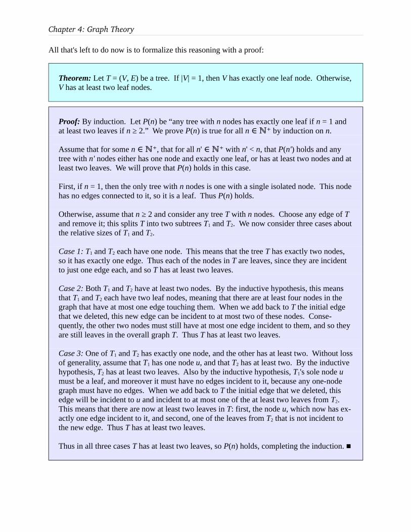
Chapter 4: Graph Theory

All that's left to do now is to formalize this reasoning with a proof:

Theorem: Let T = (V, E) be a tree. If |V| = 1, then V has exactly one leaf node. Otherwise, V has at least two leaf nodes.

Proof: By induction. Let P(n) be “any tree with n nodes has exactly one leaf if n = 1 and at least two leaves if n ≥ 2.” We prove P(n) is true for all n by induction on ∈ ℕ⁺ n.

Assume that for some n , that for all ∈ ℕ⁺ n' with ∈ ℕ⁺ n' < n, that P(n') holds and any tree with n' nodes either has one node and exactly one leaf, or has at least two nodes and at least two leaves. We will prove that P(n) holds in this case.

First, if n = 1, then the only tree with n nodes is one with a single isolated node. This node has no edges connected to it, so it is a leaf. Thus P(n) holds.

Otherwise, assume that n ≥ 2 and consider any tree T with n nodes. Choose any edge of T and remove it; this splits T into two subtrees T1 and T2. We now consider three cases about the relative sizes of T1 and T2.

Case 1: T1 and T2 each have one node. This means that the tree T has exactly two nodes, so it has exactly one edge. Thus each of the nodes in T are leaves, since they are incident to just one edge each, and so T has at least two leaves.

Case 2: Both T1 and T2 have at least two nodes. By the inductive hypothesis, this means that T1 and T2 each have two leaf nodes, meaning that there are at least four nodes in the graph that have at most one edge touching them. When we add back to T the initial edge that we deleted, this new edge can be incident to at most two of these nodes. Conse-quently, the other two nodes must still have at most one edge incident to them, and so they are still leaves in the overall graph T. Thus T has at least two leaves.

Case 3: One of T1 and T2 has exactly one node, and the other has at least two. Without loss of generality, assume that T1 has one node u, and that T2 has at least two. By the inductive hypothesis, T2 has at least two leaves. Also by the inductive hypothesis, T1's sole node u must be a leaf, and moreover it must have no edges incident to it, because any one-node graph must have no edges. When we add back to T the initial edge that we deleted, this edge will be incident to u and incident to at most one of the at least two leaves from T2. This means that there are now at least two leaves in T: first, the node u, which now has ex-actly one edge incident to it, and second, one of the leaves from T2 that is not incident to the new edge. Thus T has at least two leaves.

Thus in all three cases T has at least two leaves, so P(n) holds, completing the induction. ■

219 / 347

This proof makes it possible for us to inductively prove results about trees in a different way. Because each tree has at least one leaf, we can proceed using weak induction on the number of nodes in the tree as follows:

• Prove the base case directly for the one-node tree.

• Prove the inductive step by starting with an (n+1)-node tree, removing a leaf, and then applying the inductive hypothesis to the n-node tree that remains.

4.2.4 Directed ConnectivityThis section on graph connectivity has primarily focused on undirected graphs and undirected connectivity. What happens if we focus instead on directed graphs? How does this affect our definition of connectivity?

To motivate this discussion, suppose that you are laying out streets in a city and want to make the streets one-way. You want to ensure that it's possible to get from any location in the city to any other location in the city without going the wrong way on any street. How should you lay out the streets?

This is not as simple as it might look. For example, suppose that the locations in the city are laid out as follows:

A

G H

B C

I J

D

K

E

L

F

Now, consider the following way of laying out roads:

A

G H

B C

I J

D

K

E

L

F

Notice that it's not always possible to get to any intersection to any other intersection. For exam-ple, you cannot get to location A starting from location C. This road network has the property that if you ignore directionality, the city is connected (in an undirected connectivity sense), but it is not connected if you are forced to follow the one-way streets.

A better layout would be this one, where every location is reachable from every other location:

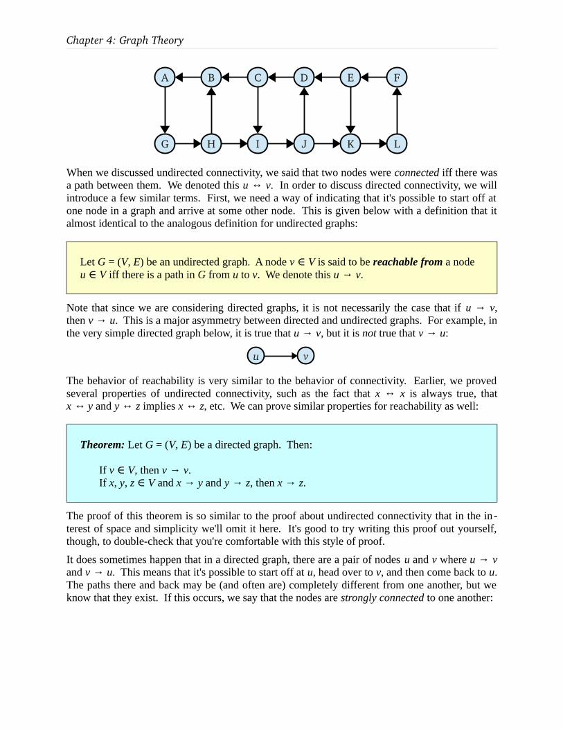
Chapter 4: Graph Theory

A

G H

B C

I J

D

K

E

L

F

When we discussed undirected connectivity, we said that two nodes were connected iff there was a path between them. We denoted this u ↔ v. In order to discuss directed connectivity, we will introduce a few similar terms. First, we need a way of indicating that it's possible to start off at one node in a graph and arrive at some other node. This is given below with a definition that it almost identical to the analogous definition for undirected graphs:

Let G = (V, E) be an undirected graph. A node v ∈ V is said to be reachable from a node u ∈ V iff there is a path in G from u to v. We denote this u → v.

Note that since we are considering directed graphs, it is not necessarily the case that if u → v, then v → u. This is a major asymmetry between directed and undirected graphs. For example, in the very simple directed graph below, it is true that u → v, but it is not true that v → u:

u v

The behavior of reachability is very similar to the behavior of connectivity. Earlier, we proved several properties of undirected connectivity, such as the fact that x ↔ x is always true, that x ↔ y and y ↔ z implies x ↔ z, etc. We can prove similar properties for reachability as well:

Theorem: Let G = (V, E) be a directed graph. Then:

If v ∈ V, then v → v.If x, y, z ∈ V and x → y and y → z, then x → z.

The proof of this theorem is so similar to the proof about undirected connectivity that in the in-terest of space and simplicity we'll omit it here. It's good to try writing this proof out yourself, though, to double-check that you're comfortable with this style of proof.

It does sometimes happen that in a directed graph, there are a pair of nodes u and v where u → v and v → u. This means that it's possible to start off at u, head over to v, and then come back to u. The paths there and back may be (and often are) completely different from one another, but we know that they exist. If this occurs, we say that the nodes are strongly connected to one another:

221 / 347

If u and v are nodes in a directed graph, we say that u and v are strongly connected iff u → v and v → u. If u and v are strongly connected, we denote this as u ↔ v.

The fact that we use the ↔ symbol to mean both “connected in an undirected graph” and “strongly connected” might seem a bit odd here, but conceptually they mean the same thing. Af-ter all, in an undirected graph, if there's a path from u to v, there is guaranteed to be a path back from v to u.

Many properties of undirected connectivity also hold for directed connectivity, as evidenced by this theorem:

Theorem: Let G = (V, E) be a directed graph. Then:

If v ∈ V, then v ↔ v.If u, v ∈ V and u ↔ v, then v ↔ u.If x, y, z ∈ V and x ↔ y and y ↔ z, then x ↔ z.

As above, this proof is so similar to the proof for directed connectivity that we will omit it. You can prove this theorem using the properties of → that we listed above, and doing so is a reason-ably straightforward exercise.

Given our definition of strong connectivity, we can define what it means for all nodes in a di -rected graph to be reachable from one another:

A directed graph G = (V, E) is called strongly connected iff for any u, v ∈ V, that u ↔ v.

For example, the graph on the left is strongly connected, while the graph on the right is not:

So far, our discussion of strong connectivity has paralleled our discussion of undirected connec-tivity. One of the interesting properties of undirected connectivity that we explored were con-nected components, regions of an undirected graph that are connected to one another. The con-nected components of a graph, intuitively, formed “pieces” of the graph. Can we extend this def-inition to strongly connected components?

Chapter 4: Graph Theory

To motivate this, suppose that you live in a city whose roads have been very poorly planned. All of the streets are one-way streets, but not every location is reachable from every other location. As a result, if you go driving, there is no guarantee that you'll be able to get back to where you started from. For example, let's suppose that the roads are laid out like this:

A

G H

B C

I J

D

K

E

L

F

Let's suppose that you start at location C. Suppose that you want to go out for a drive, but don't want to go anywhere from which you can't get back to where you started. Where could you safely go? With a bit of thought, you can see that these locations are the ones indicated here:

A

G H

B C

I J

D

K

E

L

F

The reason for this is as follows. Any of the locations A, B, C, or D can't be reached from where you're starting, so there's no possible way that you could go there. Any of the locations E, F, K, or L can be reached from C, but if you go to them you'll not be able to return from where you started. The remaining locations are reachable from your starting point, and have a return back back to the start.

If you think about the nodes that you can visit, they're precisely the nodes that are strongly con-nected to your initial starting point. All of the other nodes in the graph, for some reason or an-other, aren't strongly connected to C. Consequently, you either can't visit them, or can't visit them and return to your starting point. In other words, you can think of the set of nodes that you can reach from C as the set

S = { v ∈ V | v ↔ C }

Does this set definition seem familiar from anywhere? If you'll recall, when we were discussing connected components, we ended up proving that every node in a graph belongs to a connected component by constructing sets that look almost identically the same as the above set, though with ↔ referring to undirected connectivity rather than strong connectivity. In a sense, the above set forms a “strongly connected” component, a group of nodes mutually reachable from one an-other. In fact, that's precisely what it is.

When discussing connected components, our goal was to break a graph down into a set of smaller “pieces.” To define what a “piece” was, we reasoned that it would be a maximal set of nodes that were all connected to one another. What if we repeat this analysis for directed

223 / 347

graphs? Our goal this time will be to split the graph into smaller “pieces” based on connectivity, except this time we will use strong connectivity, since this is a directed graph, rather than undi-rected connectivity. This gives rise to the following definition:

Let G = (V, E) be an directed graph. A strongly connected component (or SCC) of G is a nonempty set of nodes C (that is, C ⊆ V), such that

(1) For any u, v ∈ C, we have u ↔ v.(2) For any u ∈ C and v ∈ V – C, we have u ↮ v.

This definition is identically the same as the definition of a normal (undirected) connected com-ponent, except that we have replaced connectivity with strong connectivity.

Right now all we have is a definition of a strongly connected component without much of a feel for what they are. To get a better intuition for strongly connected components, let's return to our initial example of driving around a badly-planned city. We recognized that, starting at C, we could not necessarily drive anywhere and then drive back, either because we couldn't drive to the destination at all, or because if we did drive there, we'd get stuck and unable to drive back. The set of nodes reachable from our starting point formed a strongly connected component, which we saw here:

A

G H

B C

I J

D

K

E

L

F

However, this isn't the only strongly connected component in the graph, and in fact there are two more of them, which are shown here:

A

G H

B C

I J

D

K

E

L

F

Notice how all the nodes in a strongly connected component are mutually reachable from one an-other. Also notice that in the above graph, every node belongs to exactly one strongly connected component. It turns out that the following theorem is true, and the proof is pretty much the same one we had for normal undirected connected components:

Chapter 4: Graph Theory

Theorem: Every node in a directed graph G belongs to exactly one strongly connected component.

This theorem implies that no two strongly connected components can overlap one another. This means that we can think about the structure of how the strongly connected components of a graph relate to one another. This is a fascinating topic, and we'll cover it later in this chapter.

4.3 DAGsThe idea of a graph is very general and encompasses many different types of structures – it can encode both the connections in the human brain and preferences for different types of food. Of-ten, it is useful to focus on specific types of graphs that are useful for encoding particular con-nections between objects. Much of this chapter will focus on specific sorts of graphs and their applications. This particular section focuses on one type of graph called a directed acyclic graph that arises in many contexts in computer science.

Let's suppose that you are interested in making pancakes. Here is a simple pancake recipe taken from allrecipes.com:*

1 1/2 cups all-purpose flour 1 tablespoon white sugar

3 1/2 teaspoons baking powder 1 1/4 cups milk

1 teaspoon salt 1 egg

3 tablespoons butter, melted

In a large bowl, sift together the flour, baking powder, salt and sugar. Make a well in the center and pour in the milk, egg and melted butter; mix until smooth.

Heat a lightly oiled griddle or frying pan over medium high heat. Pour or scoop the batter onto the griddle, using approximately 1/4 cup for each pancake. Brown on both sides and serve hot.

Now, suppose that you and your friends are interested in making a batch of these pancakes. To do so, you need to distribute the tasks involved in the recipe. You'd like the work to be distrib-uted in a way where the job will get finished as fast as possible. How would you distribute these tasks?

Let's think of what tasks are involved in this recipe:

• Measure the flour, baking powder, salt, sugar, and milk.

• Melt the butter.

• Beat the egg.

• Combine dry ingredients.

* Taken from http://allrecipes.com/recipe/good­old­fashioned­pancakes/, accessed on 21 July, 2012.  Recipe highly recommended.

225 / 347

• Mix in wet ingredients.

• Oil the griddle.

• Head the griddle.

• Make pancakes.

• Serve pancakes.

For you and your friends to make these pancakes as quickly as possible, you would probably want to work on a lot of these tasks in parallel. For example, while one person measures the flour, another could beat the egg, measure milk, etc. However, not all tasks can be run in paral-lel. For example, you can't mix in the wet ingredients at the same time that you're measuring the dry ingredients, since those ingredients need to be combined together first. Similarly, you can't serve the pancakes at the same time that you're melting the butter, since there aren't any pancakes yet to serve!

The issue is that some of the above tasks depend on one another. Given that this is the case, you want to find a way to get as much done in parallel as possible, subject to the restriction that no task is performed until all of its prerequisite tasks have been taken care of first.

So how exactly do we do this? As with much of mathematics and computer science, we will do this in two steps. First, let's see what mathematical structures we might use to model the prob-lem. Once we have that model, we can then analyze it to find the most efficient way of paral-lelizing the tasks.

As you might have guessed, we will formalize the cooking constraints as a graph. Specifically, we'll use a directed graph where each node represents a task, and there is an edge from one task to another if the second task directly depends on the first. Here is what this graph would look like for our cooking tasks:

MeasureFlour

MeasureBaking Powder

MeasureSalt

MeasureSugar

MeasureSugar

MeasureMilk

Melt Butter

Beat Egg

CombineDry Ingredients

Oil Griddle

HeatGriddle

Add WetIngredients

MakePancakes

ServePancakes

Chapter 4: Graph Theory

Given this graph, it's a lot easier to see how we might parallelize the tasks. If you have a total of five people working on pancakes, you could distribute the tasks as follows: initially, have every-one work on measuring one of the dry ingredients. Next, have someone combine everything, one person work on each liquid ingredient, and one person oil the griddle. As a next step, have someone heat the griddle while someone else combines everything. Then, make the pancakes, and then serve them. This process is about as efficient as it gets – pretty much everyone is work-ing on something up until there aren't enough tasks left to go around!

The important thing to note about the above graph is that it is indeed possible to perform all the tasks in some order. Although there are dependencies in the graph, there is one way of ordering the tasks so that there are no conflicts. Consequently, we eventually do get to eat our pancakes.

Let's now switch gears and consider a totally different example. Suppose that you have a set of classes that you need to take (say, because you're interested in doing a CS major or CS minor) and want to find out what order you should take your classes in. You have before you the list of classes you want to take, along with their prerequisites. For example, in the Stanford CS depart-ment, you might have this set of classes:

Number Title Description Prerequisites

CS103 Mathematical Foundations of Computing

Discrete math, proof techniques, computability, and complexity.

CS106A

CS106A Programming Methodology

Introduction to computer programming and software engineering in Java.

None

CS106B Programming Abstractions Data structures, recursion, algorithmic analysis, and graph algorithms.

CS106A

CS107 Computer Organization and Systems

Data representations, assembly language, memory organization.

CS106B

CS109 Introduction to Probability for Computer Scientists

Combinatorics, probability, independence, expectation, and machine learning.

CS103, CS106B

CS110 Principles of Computer Systems

Software engineering techniques for computer systems.

CS107

CS143 Compilers Techniques in compiler construction and code optimization.

CS103, CS107

CS161 Design and Analysis of Algorithms

Big-O, recurrences, greedy algorithms, randomization, and dynamic programming.

CS103, CS109

227 / 347

How would you order these classes so that you can take all of them without violating any of the prerequisites? Just looking over this table, it's a bit tricky to see a valid ordering (unless you al-ready happen to know one). However, if we represent these dependencies as a graph, it becomes a lot easier to find a legal structure. As before, we'll build a graph where each node represents a class, and an edge from one class to another means that the second class has the first as a prereq-uisite. If we do this, we get the following graph:

CS106A

CS106B

CS103 CS109

CS107 CS110

CS143

CS161

From here, we can start seeing how to order the courses. For example, one ordering would be to do CS106A first, then CS106B and CS103 in parallel, then CS107 and CS109, followed by CS110, CS143, and CS161. Of course, that's a pretty crazy course schedule, so you could also take the more reasonable CS106A, then CS106B, then CS103, then CS107, then CS109, then CS161, and finally CS143.

As with the baking question, this graph has the nice property that even though there are depen-dencies between courses, the courses can indeed be ordered such that they can all be completed in order. Not all course schedules have this property; here's one possible class schedule where it's impossible to take all classes with their prerequisites, courtesy of Randall Munroe:*

4.3.1 Topological OrderingsBoth of the previous examples – baking tasks and course scheduling – were easily modeled as dependency graphs, where nodes and edges correspond to restrictions on how various objects can be ordered. The essential properties of these graphs were the following:

* http://xkcd.com/754    

Chapter 4: Graph Theory

• The graphs were directed, so that dependency orders could be enforced, and

• There was some order in which the tasks could be completed without breaking any de-pendencies.

We already have a formalization for the first of these requirements (directed graphs). Can we formalize this second constraint? Using the new language of graph theory, it turns out that it is possible to do so.

Let G = (V, E) be a directed graph. A topological ordering of G is an ordering v1, v2, …, vn

of the nodes in G such that if i ≤ j, then there is no edge from vj to vi.

Don't let the term “topological ordering” throw you off; this definition is not as complex as it may seem. Stated simply, a topological ordering is a way of listing off all the nodes in a graph so that no node is listed before any of the nodes that it depends on. For example, in the class listing example, a topological ordering corresponds to a sequence of classes that you can take while re-specting prerequisites, while in the case of cooking a topological ordering is a way of performing all the steps in the recipe without performing any one task before all the others it depends on.

Not all graphs have topological orderings. For example, neither of these graphs can be topologi-cally ordered:

B

A

C

ED F

D

F G

C E

A B

Intuitively, the graph on the left can't be topologically ordered because no matter how you try to order the nodes B, C, D, and E, one of the nodes will have to come before one of the nodes it de-pends on. Similarly, the graph on the right has the same problem with the nodes D, E, and F.

What sorts of graphs do have a topological ordering? Graphs with these properties arise fre-quently in computer science, and we give them a special name: the directed acyclic graph.

A directed acyclic graph, or DAG for short, is a directed graph containing no cycles.

Let's take a minute to look at exactly what this means. We've talked about directed graphs be-fore, but what about “acyclic” graphs? If you'll recall, a cycle in a graph is a series of nodes that trace out a path from some node back to itself. An acyclic graph is graph that contains no cycles. Intuitively, this means that if you trace out any path in the graph starting from any node, there is no possible way to return to where you have started.

229 / 347

Both of the dependency graphs from before are DAGs – you can verify this by trying to find a path from any node back to itself – as are the following graphs:

A B C

FED

IHG

C

A

D

E

B

However, these graphs from before, which have no topological orderings, are also not DAGs:

B

A

C

ED F

D

F G

C E

A B

Right now, we have two completely different definitions. On the one hand, we have topological orderings, which talk about a way that we can order the nodes in a graph. On the other hand, we have DAGs, which talk about the structural properties of graphs. When defining DAGs, we claimed that DAGs are precisely the graphs that admit a topological ordering. Why exactly is this? How do we connect orderings of nodes to cycles?

To prove that this is true, we will prove two theorems that, taken together, establish that a graph is a DAG iff it has a topological ordering.

Theorem: Let G be a directed graph. If G has a topological ordering, then G contains no cycles.

Theorem: Let G be a directed graph. If G contains no cycles, then G has a topological or-dering.

The rest of this section is dedicated to proving each of these results.

We will first prove that if a graph has a topological ordering, then it must be a DAG. This proof is actually not too difficult. The idea is as follows: rather than proving this directly, we'll use the contrapositive, namely, that if a graph contains a cycle, then it cannot have a topological order-ing. Intuitively, you can think about this by considering a set of classes whose dependencies form a cycle. That is, class A depends on class B, which depends on class C, which eventually in turn depends again on class A. No matter how you try to order the classes, whichever class you try to take first must have some prerequisite that you haven't taken yet.

We can formalize this using the following proof.

Chapter 4: Graph Theory

Theorem: Let G be a directed graph. If G has a topological ordering, then G contains no cycles.

Proof: By contrapositive; we will show that if G contains a cycle, then G does not have a topological ordering.

Consider any graph G containing a cycle C; let that cycle be (v1, v2, …, vk, vi). Now, con-sider any way of ordering the nodes of G. Consider the very first node vi of the cycle that appears in this ordering, and let it be at position r in the ordering. Let vj be the node that comes before vi in the cycle, and let its position in the ordering be s. Since vi is the earliest node of the cycle to appear in the ordering, we know that r ≤ s. However, since vj immedi-ately precedes vi in the cycle, there must be an edge from vj to vi. Consequently, this order-ing of the nodes cannot be a topological ordering. Since our choice of ordering was arbi-trary, this means that any ordering of the nodes of G is not a topological ordering. Thus G has no topological orderings, as required. ■

Notice how this proof is put together. We start off by identifying the cycle that we want to con-sider, and then think about any arbitrary ordering. We know that every node in the cycle must appear somewhere in this ordering, so there has to be a node in the cycle that appears in the or-dering before any other node in the cycle (this is the node vi). This means that every node in the cycle must appear after vi in the ordering. In particular, this means that the node that precedes the vi in the cycle (which we'll denote vj) must come after vi in the ordering. Therefore, the or-dering can't be a topological ordering; there is an edge from vj to vi, even though vi comes before vj.

An important detail of this proof is that we chose the earliest node in the ordering that appeared in the cycle. This made it possible to guarantee that the node that comes before it in the cycle must appear later on in the ordering than it. This is an excellent application of the well-ordering principle. If we picked an arbitrary node in the cycle, there is no guarantee that anything imme-diately connected to it would cause a problem for the topological ordering.

The second proof – that any DAG has a topological ordering – is more involved than our previ-ous proof. In order to prove this result, we will have to explore the properties of DAGs in more depth.

Intuitively, why is it always possible for us to topologically order the nodes of a DAG? To see why, let's consider an example. Consider the course prerequisites DAG from earlier in this chap-ter:

231 / 347

CS106A

CS106B

CS103 CS109

CS107 CS110

CS143

CS161

If we want to topologically order the nodes of this graph, we would have to start off with CS106A, since everything in the graph depends on it. Once we've taken that course, we're left with

CS106B

CS103 CS109

CS107 CS110

CS143

CS161

Now, we can take either CS106B or CS103. Let's suppose that we want to take CS103 next. This leaves

CS106B

CS109

CS107 CS110

CS143

CS161

Now, we have to take CS106B. Doing so leaves

Chapter 4: Graph Theory

CS109

CS107 CS110

CS143

CS161

So we can now take CS107 or CS109. Iterating this process over and over again will eventually give us a topological ordering of the graph.

Notice that at each point in this process, we are always able to find a node in the DAG that has no incoming edges. We can then take that node out of the DAG, place it next in the topological ordering, and then repeat this process over and over again. Eventually, we'll be left with a topo-logical ordering.

To formalize this, let us introduce a few important definitions:

Given a DAG G, a source in G is a node with no incoming edges. A sink is a node with no outgoing edges.

For example, in the graph of CS courses, CS106A is a source, while CS110, CS161, and CS143 are sinks.

Our previous discussion about topological orderings of DAGs can now be restated as follows: if the graph is a DAG, we can always find a source node in it. We can then remove it, place it at the front of our topological ordering, and repeat the process on what remains. Assuming that this is possible, it gives us a proof that any DAG has a topological ordering. Moreover, it gives us a constructive algorithm we can use to find a topological ordering – repeatedly find a source node and remove it from the graph.

To justify this algorithm, we need to introduce two key lemmas:

Lemma 1: If G is a DAG with at least one node, G has at least one source.

Lemma 2: If G is a DAG with at least one source node, the graph G' formed by removing that source node from G is also a DAG.

These lemmas, taken together, can be used to prove that any DAG has a topological ordering (we'll go over that proof at the end of this section). In the meantime, let's work through the proofs of both of these lemmas.*

* Did you know that the plural of lemma is lemmata?  You are now part of the .01% of people that know this scintillating fact!

233 / 347

First, how would we show that every DAG with at least one node has at least one source? In a sense, this seems obvious – any DAG that we can try must have this property. But to formally prove this, we'll need a stronger argument.

Let's see what we have to work with. The definition of a DAG is pretty minimal – all we know is that it's a directed graph with no cycles. If we want to show that this means that it has at least one source node, we'll have to somehow base that on the fact that it has no cycles. How might we use this fact? Well, one option would be to try a proof by contrapositive. Could we show that if a (nonempty) graph has no sources, then it cannot be a DAG? If it's not a DAG, that means that it must have a cycle in it. So now we have something to work with: let's try to prove that if a nonempty graph has no sources, then it cannot be a DAG.

Now, what can we say about a graph with no sources? Since the graph has no sources, we know that every node in the graph must have some incoming edge. In other words, starting at any node in the graph, we could walk backwards across the edges of the graph without ever getting stuck, because no matter what node we end up at, we are always able to walk backward one more step.

It's here where we can spot something fishy. Suppose that there are n nodes in our graph. Start at any one of them, and take n + 1 steps backwards. In the course of doing so, you will have vis-ited n + 1 nodes. But all these nodes can't be different, since there are only n total nodes in the graph! Consequently, we had to have visited the same node twice. If that's the case, the path that we've traced out must have contained a cycle, because at some point we entered a node, followed some nodes, then reentered that node again. (Technically speaking we traced that cycle out in re-verse, but it's still a cycle).

We can formalize this intuition here:

Lemma 1: Any DAG with at least one node contains a source.

Proof: Let G be a nonempty graph. We will prove that if G is a DAG, then G contains a source by contrapositive; we instead show that if G has no sources, then G is not a DAG. Since G contains no sources, there are no nodes in G that have no incoming edges. Equiv-alently, every node in G has at least one incoming edge.

Let n be the total number of nodes in G. Now, starting from any node in G, begin follow-ing some edge entering G in reverse. We will always be able to do this, since every node has at least one incoming edge. Repeat this process n + 1 times to get a series of nodes vn+1, vn, …, v1 traced out this way. In other words, the sequence v1, v2, …, vn+1 is a path in G.

Now, since there are n + 1 nodes in this path and only n different nodes in the graph, the sequence v1, v2, …, vn+1 must contain at least one duplicate node. Let vi be the first occur-rence of this duplicated node and vj be the second, with i ≤ j. Then the path vi, vi+1, …, vj starts and ends at the same node, so it is a cycle in G. Since G contains a cycle, it is not a DAG, which is what we wanted to show. ■

Chapter 4: Graph Theory

The third paragraph of the above proof is the key step. It works by arguing that since we have visited n + 1 nodes in our path, but there are only n total nodes in the graph, that we must have visited some node twice, from which we can derive the cycle. This is an example of a technique called the pigeonhole principle, a powerful technique in discrete mathematics. We will explore this technique in more depth in a later chapter.

With this lemma in hand, we now know that any nonempty DAG must have at least one source node. It turns out that DAGs can have many source nodes; as an example, here's a DAG where all but one of the nodes are sources:

A

F

B C D E

The next step in our proof is to show that if we peel off any source node from a DAG, what we're left with is a DAG. This proof is much easier than the previous one. The intuition is that if we start off with a graph that contains no cycles and then start removing nodes from it, we can't ever introduce a cycle. This is formalized below:

Lemma 2: Let G be a DAG with source node v. Then the graph G' formed by removing v and all its outgoing edges is a DAG.

Proof: By contradiction; assume that there is a DAG G with source node v, but that G' contains a cycle. Let that cycle C be x1, x2, …, xk, x1. Since G' is G with the node v re-moved, we know that v ∉ C. Consequently, all of the nodes xi and their corresponding edges must also be in G, meaning that C is also a cycle in G. But this is impossible, since G is a DAG. We have reached a contradiction, so our assumption must have been wrong and G' must also be a DAG. ■

Now, we can combine both of these lemmas together to prove that any DAG has a topological ordering. To do so, we'll show that if you iteratively remove a source node and place it next in the ordering, then eventually you will build a topological ordering for the DAG. Since this process is iterative and keeps shrinking the DAG, our proof will be inductive on the number of nodes in the DAG.

Theorem: Any DAG G has a topological ordering.

235 / 347

Proof: By induction; let P(n) be “any DAG with n nodes has a topological ordering.” We will prove P(n) is true for all n by induction.∈ ℕ

As our base case, we prove P(0), that any DAG with 0 nodes has a topological ordering. This is true because a DAG with no nodes has a trivial topological ordering – just list all 0 of its nodes in order.

For the inductive step, assume that P(n) holds for some n , meaning that any DAG ∈ ℕwith n nodes has a topological ordering. We then prove P(n + 1), that any DAG with n + 1 nodes has a topological ordering. Consider any DAG G with n + 1 nodes; since this DAG is nonempty, it must have at least one source node. Pick any such source and call it v0. We can then remove s from G to form a new DAG G' with n nodes. By our inductive hypothe-sis, this DAG has a topological ordering v1, v2, …, vn.

Now, order the nodes of G as v0, v1, v2, …, vn. We claim that this is a topological ordering of G. First, we can see that every node of G appears exactly once in this ordering – if the node is v0, it's at the front of the ordering, and every other node appears once as some vi. Next, we show that for any nodes vi and vj, if i ≤ j, then there is no edge from vj to vi. To see this, we consider two cases:

Case 1: i = 0. Since v0 is a source, it has no incoming edges. Thus there cannot be any edges from vj to v0 for any j.

Case 2: i > 0. Since 0 < i ≤ j, we know that 1 ≤ i ≤ j. Consequently, both vi and vj are nodes in G'. Since v1, v2, …, vn is a topological ordering of G', this means that there is no edge from vj to vi.

Thus in either case we have that there are no edges from vj to vi for any choice of i and j. Consequently, v0, v1, …, vn is a topological ordering of G. Since our choice of G was arbi-trary, this means that any DAG with n + 1 nodes has a topological ordering, completing the proof. ■

As a fitting coda to this section, notice that we have just proved that there is a topological order-ing of a set of tasks (that is, a way of accomplishing all the tasks in some order) precisely when no tasks have circular dependencies. This might seem obvious, but it's always reassuring when we can use the vast power of mathematics to confirm our intuitions!

4.3.2 CondensationsAs hinted at in the section about strongly connected components (SCCs), the ways in which strongly connected components relate is actually quite interesting. This section explores exactly what structures arise when we consider the connections between SCCs.

Consider, for example, the following graph, whose SCCs have been outlined:

Chapter 4: Graph Theory

If you'll notice, there are some nodes in the leftmost SCC with edges to the top-middle SCC. There is also a node in the right SCC with an edge to the top-middle SCC, as well as a node with an edge to the bottom-middle SCC. The top-middle SCC in turn has several nodes with edges to the bottom-middle SCC. In this sense, we can think of various SCCs being linked directionally – one SCC might have edges from it that arrive in another SCC.

Given this idea as a starting point, we can consider a somewhat unusual idea. What if we were to construct, from the above graph, a new graph showing the original graph's SCCs and the connec-tions between them? To do this, we would proceed as follows. Each node of this new graph will represent an SCC of the original graph. We will then add directed edges between two SCCs if there is a node in the first SCC with an edge to a node in the second SCC. Intuitively, you can think of this as follows. Draw a border around all of the strongly-connected components in the graph. After doing this, there might be some edges in the graph that start inside an SCC, but then cross the border into another SCC. These edges are then converted into new edges that run from the first SCC into the second.

As an example, given the above graph, we would construct the graph of its SCCs as follows:

Here is another example of a graph, its SCCs, and the resulting graph:

237 / 347

Some directed graphs have very uninteresting SCCs consisting of just a single node each. In that case, the resulting graph is the same as the original. You can see this here:

On the other hand, some graphs have just one SCC, in which case the graph of the SCCs is just a single node:

Our goal in this section will be to analyze the properties of the graphs formed this way and to reason about their properties. Doing so ends up giving up some interesting insights into the structure of arbitrary directed graphs. But first, we need to formalize how we're constructing the above graph.

It turns out that formalizing this construction is not challenging, but can become notationally quite messy. In order to describe the graph of SCCs, we need to define what the nodes and edges of that graph are. So let's take an arbitrary directed graph G = (V, E) as our starting point. From here, we will define two sets V' and E' that will be the nodes and edges of the new graph that we will form.

Of the two sets V' and E', the set V' is easiest to define. Since we want a graph of all the SCCs in the original graph, we can just define V' to be the SCCs of the original graph. More specifically, we'll say that

V' = { S | S is an SCC of G }

It may seem strange that the nodes in our new graph are sets of nodes from the original graph, but that's precisely what we're doing. Remember that the mathematical definition of a graph just says that we need a set of objects to act as nodes and a set of objects to act as edges. The objects that acts as nodes can be anything, including sets of other objects that themselves act as nodes in

Chapter 4: Graph Theory

another graph. When drawing out the nodes of the new graph that we'll form, I will usually not draw each node as if it's an SCC of the original graph, but I will try to give some indication that the nodes themselves are sets.

Now, we need to come up with a set of edges. This ends up being a bit trickier. Our intuition for the edges in the new graph was to take each edge whose nodes crossed from one SCC to another, then to convert that edge to an edge between the corresponding SCCs. Formally speaking, we're saying that there is an edge from SCC S1 to SCC S2 iff some node in S1 has an edge to some node in S2. If we were to write this out in set-builder notation, we might attempt to do so as follows:

E' = { (S1, S2) | There exists u ∈ S1 and v ∈ S2 such that (u, v) ∈ E }

(Here, E is the original edge set from the graph.) Unfortunately, this definition doesn't quite give us what we want. In particular, let's see what this definition would have us do on the following graph:

This graph is strongly connected, so there's just one SCC, which encompasses all the nodes. However, notice that there are plenty of edges between nodes in this SCC. If we look at the lit -eral definition of E', we should therefore have that in the SCC graph of the graph above, there is an edge from the SCC to itself. Under the current definition, this means that we'd get the graph on the left as our SCC graph, rather than the graph on the right (which is more what we intended):

As a result, we'll add one more constraint to our set of edges. Not only must there be an edge crossing from the first SCC to the second, but the two SCCs themselves must not be the same. This looks as follows:

E' = { (S1, S2) | S1 ≠ S2, and there exists u ∈ S1 and v ∈ S2 such that (u, v) ∈ E }

Great! We now have a formal definition of the nodes and edges of our SCC graph. These two definitions, taken together, give us the following:

239 / 347

Let G = (V, E) be a directed graph. The condensation of G, denoted GSCC, is a graph of the strongly-connected components of G defined as follows:

Let V' = { S | S is an SCC of G }Let E' = { (S1, S2) | S1 ≠ S2, and there exists u ∈ S1, v ∈ S2 such that (u, v) ∈ E }

Then GSCC = (V', E').

Note that we'll use the notation GSCC to describe the graph that we get from the SCCs of G, which as mentioned above is called the condensation of G.

And now for a pretty neat observation about condensations. Take a look at all of the condensa-tions that we have seen so far. Interestingly, not a single one of them contains a cycle. This is particularly interesting, because it means that the structure of all of these graphs, most of which contain cycles, can be reduced down to DAGs, where each node is a strongly connected compo-nent of the original graph. If it turns out that this is true in general, and that the condensation of any graph G is guaranteed to be a DAG, it shows that DAGs are a fundamentally important class of graph.

It turns out that, indeed, the above result is no coincidence, and in fact holds for all graphs. For-mally, we have the following theorem:

Theorem: For any directed graph G, the graph GSCC is a DAG.

Proving this theorem will require us to first gain an understanding about why this result is true, and second to build up the mathematical machinery necessary to prove it.

Let's start off with an intuition. Why must all condensations be DAGs? This has to do with the definition of an SCC. Recall that an SCC is, informally, a cluster of nodes that are all strongly connected to one another that cannot be grown any further. This means that if we pick any SCC from a graph and choose any node v outside that SCC, then none of the nodes in the SCC are strongly connected to v. This means that either there is no path from any of the nodes in the SCC to v, or that there is no path from v to any of the nodes in the SCC, or possibly both.

So now let's think about what it would mean if there was a condensation that wasn't a DAG. This graph would have to have a simple cycle in it, meaning that we could start off at one SCC, trace a path out to another SCC, and then trace a path back to the original SCC. For example:

Chapter 4: Graph Theory

Let's think about what this means. Consider the first edge of the path, which goes from one SCC to the next. This means that in the original graph, some node in the first SCC has an edge con-necting it to some node of the second SCC. Let's call these nodes u and v, with u in the first SCC and v in the second. Since all of the nodes in the first SCC are reachable from one another, this means that it's possible to get from any node in the first SCC to u, and thus from any node in the first SCC to v. Since all the nodes in the second SCC are strongly connected, it's possible to get from v to any node in the second SCC. Consequently, it's possible for any node in the first SCC to reach any node in the second SCC.

More generally, consider any path in the condensation. Any node in the first SCC in the path can reach any node in the second SCC in the path. By the same token, any node in the second SCC in the path can reach any node in the third, etc. In fact, any node in the first SCC on the path can reach any node in any of the SCCs on the path.

So what happens if the condensation isn't a DAG? Well, in that case, we'd have a simple cycle of SCCs that goes (S1, S2, …, Sn, S1), where all the Si's are SCCs of the original graph. We can then split this simple cycle into two simple paths: (S1, S2, …, Sn), which goes from S1 to Sn, and (Sn, S1) from Sn to S1. By our previous line of reasoning, this means that every node in S1 can reach every node in Sn, and that every node in Sn can reach S1. But S1 and Sn are are supposed to be SCCs, which means that either the nodes in S1 can't reach the nodes in Sn, or the nodes in Sn can't reach S1. This gives us a contradiction, meaning that we must have that the condensation is a DAG.

Let's review the structure of this proof before we formalize each individual step. First, we ar-gued that if we have a path in the condensation, then any node in the first SCC on the path can reach any node in the last SCC on the path. This means that a path in the condensation gives us a way of finding one-directional connectivity in the original graph. Second, we argued that if there is a simple cycle in the condensation, it means that two different SCCs must be mutually reach-able from each other, which causes a contradiction, because two disjoint SCCs can't be mutually reachable from one another.

Given this setup, let's prove each of these parts individually. The first part (about how a path in the condensation gives reachability information) we'll prove as a lemma for the second, which is the main theorem.

Here is the lemma we need to prove:

Lemma: Let G be a directed graph and GSCC its condensation. Then if there is a path (S1, S2, …, Sn) in GSCC, then for any u ∈ S1 and v ∈ Sn, we have u → v.

To prove this lemma, we'll proceed by induction on the length of the path. Earlier, we sketched a line of reasoning showing that any adjacent SCCs in a path must have all nodes in the second SCC reachable from any of the nodes in the first SCC. We can then iterate this logic over each edge in the path to get the desired result.

241 / 347

Proof: Consider any directed graph G = (V, E) and let GSCC be its condensation. Then, Let P(n) be “for any path (S1, S2, …, Sn) of length n in GSCC, if u ∈ S1 and v ∈ Sn, then u → v.” We prove P(n) is true for all n by induction on ∈ ℕ⁺ n.

As our base case, we prove P(1), for any path (S1) of length 1 in GSCC, that if u ∈ S1 and v ∈ S2, that u → v. Since u ∈ S1 and v ∈ S1 and S1 is an SCC, we have that u ↔ v, which implies that u → v as required.

For our inductive step, assume that for some n that ∈ ℕ⁺ P(n) holds and for any path (S1, S2, …, Sn) in GSCC, that if u ∈ S1 and v ∈ Sn, that u → v. We will prove that P(n + 1) holds, meaning that for any path (S1, S2, …, Sn, Sn+1) in GSCC, that if u ∈ S1 and v ∈ Sn+1, that u → v.

Consider any path (S1, S2, …, Sn, Sn+1) in GSCC. This means that (S1, S2, …, Sn) is also a path in GSCC. By our inductive hypothesis, this means that for any u ∈ S1 and x ∈ Sn, u → x. Since our initial path ends with (Sn, Sn+1), this edge exists in GSCC, meaning that there exists some y ∈ Sn and z ∈ Sn+1 such that (y, z) ∈ E, thus y → z. Consequently, we know that for any u ∈ S1, since y ∈ Sn, we have u → y and y → z, so for any u ∈ S1, we have that u → z. Finally, since Sn+1 is an SCC and z ∈ Sn+1, we know that for any v ∈ Sn+1 that z → v. Thus for any u ∈ S1 and for any v ∈ S2, we have that u → z and z → v, so u → v as required. Thus P(n + 1) holds, completing the induction. ■

Given this lemma, we can prove the following theorem:

Theorem: For any directed graph G, the graph GSCC is a DAG.

Proof: By contradiction; assume that there is a directed graph G for which GSCC is not a DAG. Thus GSCC must contain a simple cycle. Note that, by construction, GSCC does not contain any edges from a node to itself. Thus this simple cycle must have the form (S1, S2, …, Sn, S1), where n ≥ 2.

We can split this simple cycle into two paths (S1, S2, …, Sn) from S1 to Sn and (Sn, S1) from Sn to S1. By our lemma, this means that for any u ∈ S1 and v ∈ Sn, that u → v and v → u. Consequently, u ↔ v. But since S1 ≠ Sn, this is a contradiction, because u and v are strongly connected but in different SCCs. We have reached a contradiction, so our as-sumption must have been incorrect. Thus GSCC must be a DAG. ■

One way of interpreting this theorem is as follows. Given any directed graph G, we can con-struct G by starting with a collection of strongly connected graphs, ordering them in some way, and then adding edges between the nodes of those strongly connected graphs in a way that never adds an edge between a higher-numbered graph and a lower-numbered graph.

Chapter 4: Graph Theory

4.4 MatchingsLet's consider the following problem. Suppose that you have a group of people that you'd like to split into teams of two. Not everyone is willing to work with everyone else, though. (Although in theory we should all just get along, in this case practice lags a bit behind the theory.) If you are given all of the pairs of people who might be willing to work together, how might you pair people up in the best possible way?

To answer this question, let's begin by building up a mathematical model of the problem. Once we have this model, we can start reasoning about it, and ultimately can arrive at a clean and ele-gant solution.

The first question we have to answer is how we could represent this problem mathematically. We are given two pieces of information: first, a list of all the people we need to pair up, and sec -ond, a list of all pairs of people that might be willing to work together. With a bit of thought, we can see that this arrangement could be represented using a graph. We'll represent each person with a node, and connect by edges pairs of people that might be willing to work with one an-other. For example, here is one possible graph:

BA C

D E

G HF

In this graph, person A is comfortable working with people B, D, and F. Person H will work with either person E or G, but person C only wants to work with person E.

Our goal is to break this group of people up into pairs of people who are willing to work to-gether. We've decided to represent each possible pair as an edge, and so if we're trying to choose how to pair people up, we must be looking for a way of choosing which of these edges we want to use. However, not all sets of edges can work. For example, consider the following two possi-ble sets of edges:

BA C

D E

G HF

BA C

D E

G HF

On the left, we have a set of edges that represents a valid way of pairing up people within this group. The middle shows another way of pairing people up, though not everyone ends up being paired. The right side, however, does not give a valid pairing. The reason for this is as follows.

243 / 347

Take a look at person D. Notice that we have chosen two edges incident to her. As a result, it seems like we should pair her up with A, as well as with F. This is a problem, since we'd like to make sure that everyone is assigned to just one pair.

Given the three above cases, it's clear that certain sets of edges are “better” than others for this problem. Before we start trying to solve the problem, let's begin by defining some basic termi-nology that we can use to reason about what sets of edges are valid, and of those sets which are better than others.

First, what criteria does a set of edges have to have in order to be legal at all? Our goal is to as -sign people into pairs. As a result, we have to make sure that we don't pick two edges that share any endpoints; if we did, then someone would be assigned into two different pairs, which we do not want to allow. Consequently, we want to pick a set of edges such that no two of those edges share any endpoints. This gives rise to the following definition:

A matching in an undirected graph G = (V, E) is a set M ⊆ E such that no two edges in M share any endpoints.

By this definition, the left and center choices of edges are matchings, while the third is not. Our goal in solving this problem will be to pick the “best” matching out of the graph, for some defini-tion of “best.”

Now that we have a definition of a matching, let's see if we can think about how to categorize matchings as “better” or “worse.” One metric we could use to determine how good a matching is is the number of edges in the matching. A matching with a large number of edges pairs up a large number of people, while a matching with a small number of edges pairs up only a few peo-ple. By this criterion, the left matching above is a better matching than the center matching, since it matches more people.

In the absolute best case, we would like a matching that pairs up everyone with someone else. That way, no one is left alone. For this reason, matchings of this sort are called perfect match-ings:

A perfect matching in an undirected graph G = (V, E) is a matching M in G such that every node of G is contained in some edge of M.

For example, here is a graph and a perfect matching in that graph:

D

A C

E F

H

B

G

D

A C

E F

H

B

G

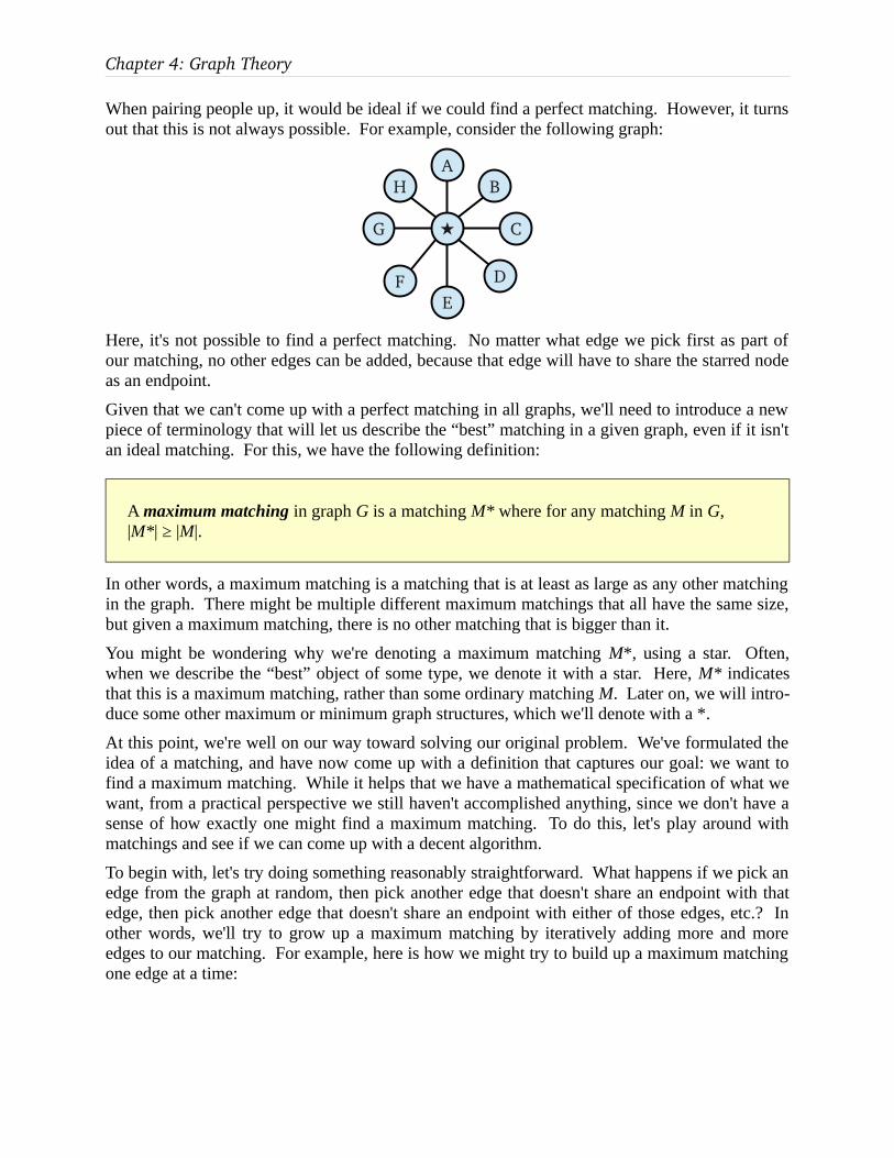
Chapter 4: Graph Theory

When pairing people up, it would be ideal if we could find a perfect matching. However, it turns out that this is not always possible. For example, consider the following graph:

G

H B

★

DE

A

F

C

Here, it's not possible to find a perfect matching. No matter what edge we pick first as part of our matching, no other edges can be added, because that edge will have to share the starred node as an endpoint.

Given that we can't come up with a perfect matching in all graphs, we'll need to introduce a new piece of terminology that will let us describe the “best” matching in a given graph, even if it isn't an ideal matching. For this, we have the following definition:

A maximum matching in graph G is a matching M* where for any matching M in G,|M*| ≥ |M|.

In other words, a maximum matching is a matching that is at least as large as any other matching in the graph. There might be multiple different maximum matchings that all have the same size, but given a maximum matching, there is no other matching that is bigger than it.

You might be wondering why we're denoting a maximum matching M*, using a star. Often, when we describe the “best” object of some type, we denote it with a star. Here, M* indicates that this is a maximum matching, rather than some ordinary matching M. Later on, we will intro-duce some other maximum or minimum graph structures, which we'll denote with a *.

At this point, we're well on our way toward solving our original problem. We've formulated the idea of a matching, and have now come up with a definition that captures our goal: we want to find a maximum matching. While it helps that we have a mathematical specification of what we want, from a practical perspective we still haven't accomplished anything, since we don't have a sense of how exactly one might find a maximum matching. To do this, let's play around with matchings and see if we can come up with a decent algorithm.

To begin with, let's try doing something reasonably straightforward. What happens if we pick an edge from the graph at random, then pick another edge that doesn't share an endpoint with that edge, then pick another edge that doesn't share an endpoint with either of those edges, etc.? In other words, we'll try to grow up a maximum matching by iteratively adding more and more edges to our matching. For example, here is how we might try to build up a maximum matching one edge at a time:

245 / 347

Notice that, at the very end, we can't add any more edges into the matching. Does this mean that it's a maximum matching? Unfortunately, the answer is no. Here is a matching in the same graph with even more edges:

A

E F G

B

JI K

H

DC

This initial attempt at an algorithm reveals something important about maximum matchings. If we have a set of edges that form a matching, and to which we can't add any more edges in the graph, we are not guaranteed that such a matching is a maximum matching. It might be a pretty good matching, but we can't be guaranteed that it's the best of all possible matchings.

To highlight the distinction between this kind of matching, where it's impossible to make any lo-cal improvements, and a true maximum matching, we introduce a new definition:

A maximal matching is a matching M in a graph G = (V, E) is a matching such that for any edge e ∈ E, either e ∈ M, or e shares an endpoint with some edge in M.

The terminology here is a bit subtle. A maximum matching is a matching that is as large as is possible in the graph. We can't do any better than a maximum matching. A maximal matching is a matching that can't be grown by adding in any edges from the graph, but which might not necessarily be as large as is possible in the graph.

A

E F G

B

JI K

H

DC A

E F

B

I K

H

DC

A B

I K

H

DC

I K

H

DCA

E F G

B

J

G

J

E F G

J

Chapter 4: Graph Theory

The distinction between maximum and maximal matchings tells us that it might to be tricky to find a maximum matching in a graph. Our naïve approach of iteratively adding in more and more edges is not guaranteed to find a maximum matching, so we will have to change our ap-proach.

Although our initial guess didn't pan out, it doesn't mean that this approach is doomed to failure. The key intuition behind this algorithm – build up a matching by continuously increasing the number of edges in it until we can't do so any more – is a good one. We just need to think a bit harder about how we might grow a fledgling matching into a maximum matching.

The reason that we can get stuck when growing a maximum matching by adding in edges is that in some cases, the only way to increase the size of a matching is to remove some edges as well. For example, here's the maximal matching that we came up with earlier:

A

E F G

B

JI K

H

DC

We can make this matching larger by removing some edges, then adding in some new edges:

A

E F G

B

JI K

H

DC A

E F G

B

JI K

H

DC

Notice that we have increased the total number of edges in the matching by one. This matching is still maximal but not maximum, but at least we've made some progress! Let's see if we can keep improving it. As before, we can grow the matching by removing some edges, and adding some new ones in:

A

E F G

B

JI K

H

DC A

E F G

B

JI K

H

DC

Once more we've increased the number of edges in the matching by one. This time, hough, we actually have a maximum matching, and we're done.

247 / 347

The above discussion shows that for this particular example, it was possible to iteratively step up the number of edges in the matching one at a time until we ultimately arrived at a maximum matching. But how on earth were we supposed to figure out what edges to add and remove at each point? And are we sure that it's always possible to step up the number of edges by one at each iteration?

To answer these questions, let's look carefully at what edges we removed and what edges we added. Below I've reprinted all of the intermediate matchings that we built up in the course of searching for a maximum matching, along with the edges that we removed (in red) and the edges that we added (in green):

A

E F G

B

JI K

H

DC A

E F G

B

JI K

H

DC

If you'll notice, there is something strange about these edges. Notice that in each case, the tog-gled edges form a path between two nodes. Moreover, those paths alternate between green (added) and red (removed) edges. Now that's odd. Is this purely a coincidence? Or is there something deeper going on here?

To answer this question, we will first need some terminology. First, let's give a name to paths like the above, which alternate between new and old edges:

Let G = (V, E) be an undirected graph and M be a matching in G. An alternating path in G is a simple path P = (v1, v2, …, vn) such that (vi, vi+1) ∈ M iff (vi+1, vi+2) ∈ E – M. An al-ternating cycle is a simple cycle C = (v1, v2, …, vn, v1) such that (vi, vi+1) ∈ M iff(vi+1, vi+2) ∈ E – M

In other words, an alternating path is a path that toggles back and forth between edges in the matching and edges not in the matching. All of the paths highlighted above are alternating paths.

In the above examples, we increased the size of a matching in the graph by finding some alter-nating path, adding in all of the edges that were not in the matching, and then removing all of the edges that were part of the original matching. Although in these cases it is possible to do this while leaving the resulting matching valid, in general we cannot take an arbitrary alternating path and update the matching by transforming it this way. For example, consider the following matching, which is maximal but not maximum. I've highlighted an alternating path in that graph:

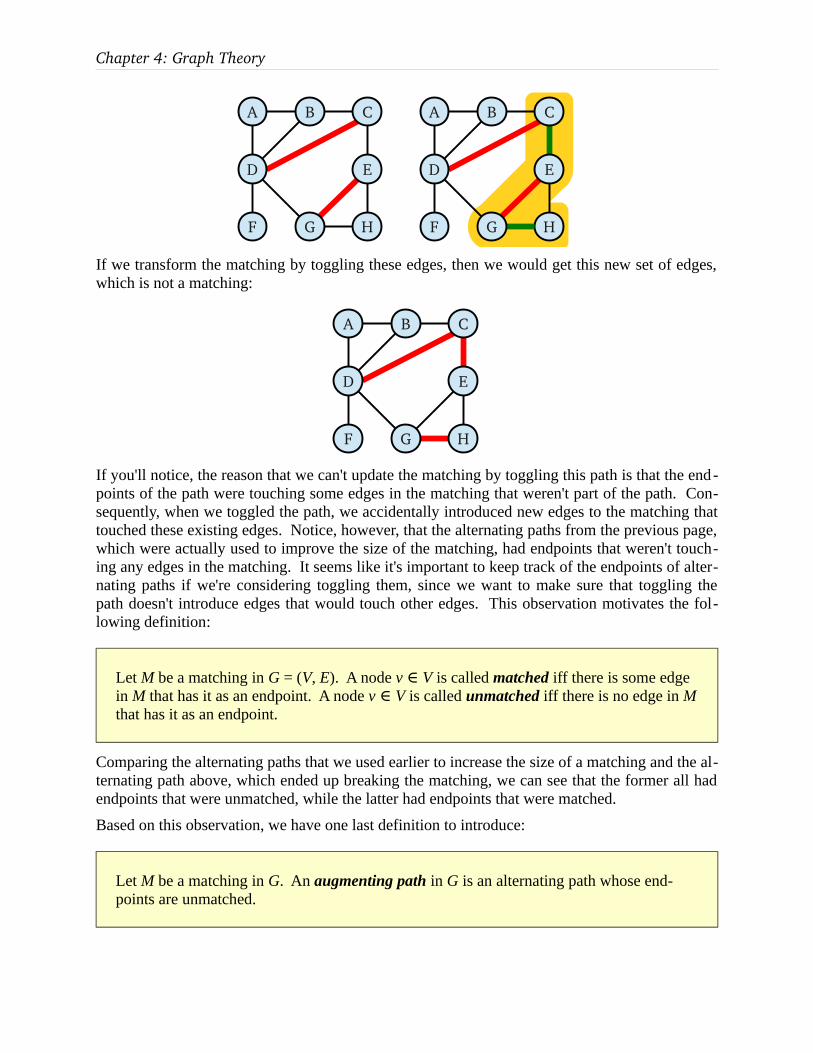
Chapter 4: Graph Theory

A B

F H

D

C

G

E

A B

F H

D

C

G

E

If we transform the matching by toggling these edges, then we would get this new set of edges, which is not a matching:

A B

F

D

H

C

G

E

If you'll notice, the reason that we can't update the matching by toggling this path is that the end-points of the path were touching some edges in the matching that weren't part of the path. Con-sequently, when we toggled the path, we accidentally introduced new edges to the matching that touched these existing edges. Notice, however, that the alternating paths from the previous page, which were actually used to improve the size of the matching, had endpoints that weren't touch-ing any edges in the matching. It seems like it's important to keep track of the endpoints of alter-nating paths if we're considering toggling them, since we want to make sure that toggling the path doesn't introduce edges that would touch other edges. This observation motivates the fol-lowing definition:

Let M be a matching in G = (V, E). A node v ∈ V is called matched iff there is some edge in M that has it as an endpoint. A node v ∈ V is called unmatched iff there is no edge in M that has it as an endpoint.

Comparing the alternating paths that we used earlier to increase the size of a matching and the al-ternating path above, which ended up breaking the matching, we can see that the former all had endpoints that were unmatched, while the latter had endpoints that were matched.

Based on this observation, we have one last definition to introduce:

Let M be a matching in G. An augmenting path in G is an alternating path whose end-points are unmatched.

249 / 347

For example, consider the following maximal matching that is not maximum. Notice that it con-tains an augmenting path, since it's an alternating path whose endpoints are unmatched:

A

D E F

B

G

C A B C

D E F

G

If we toggle this augmenting path, we get an even larger matching:

A B C

D E F

G

This matching is a maximum matching, since with three edges, a total of six nodes are covered. If we were to add another edge, we would have to cover eight nodes, but there are only six total in this graph.

Augmenting paths are the sorts of alternating paths that we want to find in a matching. If they are toggled, they definitely increase the size of the matching by one. However, the story does not end here. We can also show that if a matching is not maximum, then it has to contain an aug-menting path. This is an important result in graph theory, and we formalize it below:

Theorem (Berge): Let M be a matching in G. Then G has an augmenting path iff M is not a maximum matching.

This is a powerful result. If we have a matching that we think might be a maximum matching, then we can check if it has no augmenting paths. If it doesn't, then we know that what we have is a maximum matching. Otherwise, we can find an augmenting path, toggle it, and end up with a larger matching. This gives us an algorithm for finding maximum matchings:

• Pick any matching.

• If it has no augmenting paths, report that it is a maximum matching.

• If it has an augmenting path, toggle that path and repeat.

Chapter 4: Graph Theory

It turns out that there is a clever algorithm for doing just that called the blossom algorithm, in-vented by Jack Edmonds in 1965. This algorithm, in a technical sense that we will define in Chapter 17, is efficient. The inner workings of the algorithm are somewhat tricky, but intuitively the algorithm works by growing a maximum matching up by searching for augmenting paths and then toggling them. As a result, it's possible to efficiently solve the maximum matching problem, and in fact many important algorithms (ranging from simple resource allocation tasks to more complex algorithms for finding paths through multiple cities) use maximum matching algorithms as a subroutine.

Of course, in order to convince ourselves that this algorithm works at all, we need to formally prove Berge's theorem. This proof is quite clever, though some of the details that arise when for-malizing it are tricky. If you're interested how to prove Berge's theorem, see the next section. Otherwise, you can feel free to skip it and move on.

4.4.1 Proving Berge's Theorem ★The proof of Berge's theorem will proceed in two parts. First, we will prove that if a matching has an augmenting path, then it is not maximum. Second, we will prove that if a matching is not maximum, then it has an augmenting path. This first proof is simpler, so we'll begin with it. Our goal will be to show the following:

Theorem: Let M be a matching in G. If G has an augmenting path, then M is not a maxi-mum matching.

If you'll recall from before, we were able to increase the size of non-maximum matchings by tak-ing an augmenting path and toggling all the edges in it; every edge on the path that was previ-ously in the matching was removed, and every edge on the path that was previously not in the matching was added to the matching. Our proof of the above theorem will work by showing that given any augmenting path, performing this operation always yields a new matching with a larger number of edges than the original matching.

To do this, we will need to prove two key lemmas:

Lemma 1: Let M be a matching in G. If P is an augmenting path in G, then M Δ P is a matching in G.

Lemma 2: Let M be a matching in G. If P is an augmenting path in G, then |M Δ P| > |M|.

Before we discuss the implications of this lemma, let's quickly review what on earth this Δ sym-bol means. If you'll recall from Chapter 1, Δ is the symmetric difference operator. Given two sets, it produces the set of all elements in exactly one of the two sets. To see why this corre-sponds to our “toggling” operation, let's think about what an augmenting path looks like. From the perspective of the matching, an augmenting path looks like this:

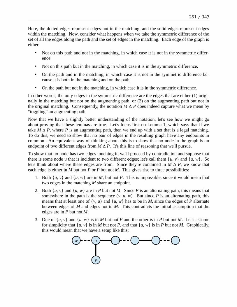
251 / 347

Here, the dotted edges represent edges not in the matching, and the solid edges represent edges within the matching. Now, consider what happens when we take the symmetric difference of the set of all the edges along the path and the set of edges in the matching. Each edge of the graph is either

• Not on this path and not in the matching, in which case it is not in the symmetric differ-ence,

• Not on this path but in the matching, in which case it is in the symmetric difference.

• On the path and in the matching, in which case it is not in the symmetric difference be-cause it is both in the matching and on the path,

• On the path but not in the matching, in which case it is in the symmetric difference.

In other words, the only edges in the symmetric difference are the edges that are either (1) origi-nally in the matching but not on the augmenting path, or (2) on the augmenting path but not in the original matching. Consequently, the notation M Δ P does indeed capture what we mean by “toggling” an augmenting path.

Now that we have a slightly better understanding of the notation, let's see how we might go about proving that these lemmas are true. Let's focus first on Lemma 1, which says that if we take M Δ P, where P is an augmenting path, then we end up with a set that is a legal matching. To do this, we need to show that no pair of edges in the resulting graph have any endpoints in common. An equivalent way of thinking about this is to show that no node in the graph is an endpoint of two different edges from M Δ P. It's this line of reasoning that we'll pursue.

To show that no node has two edges touching it, we'll proceed by contradiction and suppose that there is some node u that is incident to two different edges; let's call them {u, v} and {u, w}. So let's think about where these edges are from. Since they're contained in M Δ P, we know that each edge is either in M but not P or P but not M. This gives rise to three possibilities:

1. Both {u, v} and {u, w} are in M, but not P. This is impossible, since it would mean that two edges in the matching M share an endpoint.

2. Both {u, v} and {u, w} are in P but not M. Since P is an alternating path, this means that somewhere in the path is the sequence (v, u, w). But since P is an alternating path, this means that at least one of {v, u} and {u, w} has to be in M, since the edges of P alternate between edges of M and edges not in M. This contradicts the initial assumption that the edges are in P but not M.

3. One of {u, v} and {u, w} is in M but not P and the other is in P but not M. Let's assume for simplicity that {u, v} is in M but not P, and that {u, w} is in P but not M. Graphically, this would mean that we have a setup like this:

w u

v

Chapter 4: Graph Theory

Something has to be wrong here. Since {u, v} is in M, we know that u must be a matched node. Consequently, it can't be the endpoint of the path P. This means that there must be a node to the left and to the right of it on the path. Because the path is an alternating path, one of those edges must be in the matching. It's not {u, w}, so it must be the other edge. But then there are two different edges incident to u in the original matching, which is impossible.

Formalizing this argument pretty much means translating the above argument into more rigorous terms, which we'll do here:

Lemma 1: Let M be a matching in G. If P is an augmenting path in G, then M Δ P is a matching in G.

Proof: By contradiction; assume that M is a matching in G, P is an augmenting path in G, but that M Δ P is not a matching in G. This means that there must be some node u such that u is incident to two different edges {u, v}, {u, w} ∈ M Δ P.

Since {u, v}, {u, w} ∈ M Δ P, we have that each edge either is in M – P, or it is in P – M. We consider three cases about which edges are in which sets.

Case 1: {u, v}, {u, w} ∈ M – P. Since M – P ⊆ M, this means that {u, v}, {u, w} ∈ M. But this is impossible, since M is a matching and the two edges share an endpoint.

Case 2: {u, v}, {u, w} ∈ P – M. Since P is a simple path, this means that the sequence (u, v, w) or (w, v, u) must occur in P. But since P is an alternating path, this means that ei-ther {u, v} ∈ M or {u, w} ∈ M, which is impossible because {u, v}, {u, w} ∈ P – M.

Case 3: Exactly one of {u, v} and {u, w} belongs to P – M and one belongs to M – P. As-sume without loss of generality that {u, v} ∈ M – P and {u, w} ∈ P – M. Since P is an augmenting path, its endpoints are unmatched. Thus u cannot be an endpoint of P. Conse-quently, there must be exactly two edges along path P incident to u. Since P is an alternat-ing path, one of these edges (call it {u, x}) must be in M. Since {u, v} ∉ P, this means that x ≠ v. But then this means that {u, x} ∈ M and {u, v} ∈ M, which is impossible since M is a matching.

In all three cases we reach a contradiction, so our assumption must have been wrong. Thus M Δ P is a matching in G. ■

Great! We've established that if P is an augmenting path, then M Δ P is also a matching in G. All that remains to do is to prove Lemma 2, which states that |M Δ P| > |M|, meaning that the size of the matching has increased. Intuitively, this is true because if we take any augmenting path, like this one here:

253 / 347

The number of edges from M is one less than the number of edges not in M. Consequently, when we toggle the edges along the path, the number of edges in M increases by one. The actual de-tails of this proof are left to you as one of the chapter exercises.

Given these two lemmas, we have the following result:

Theorem: Let M be a matching in G. If G has an augmenting path, then M is not a maxi-mum matching.

Proof: Let M be a matching in G, and let P be an augmenting path. Then by Lemma 1, M Δ P is a matching in G, and by Lemma 2, |M Δ P| > |M|. Thus M is not a maximum matching. ■

We're now halfway there. We've formally proven that if you have an augmenting path, it's possi-ble to increase the size of a non-maximum matching. But now we have to prove the converse, namely, that if we have a non-maximum matching, we can always find an augmenting path. This is a beautiful proof, but it will require us to adopt a proof technique that we previously have not seen before.

The key idea behind the proof will be the following. Suppose we have an arbitrary matching M that, for whatever reason, we know is not maximum. We know that there must exist at least one maximum matching M*. We don't necessarily know anything about (how many edges it has, which edges it contains, etc.), but mathematically speaking it's fine to reason about this matching M*. Given that our matching isn't maximum, we know that there must be more edges in M* than in M. What would happen if we were to consider the “difference” between M and M*? At first this might seem like a strange idea – how can we reason about the difference between our current matching and a matching we've never seen before? – but this sort of inquiry is actually quite common in graph theory.

To give a concrete example of this, consider the following graph, along with two matchings in it:

The matching M* on the left is a maximum matching, while the matching M* on the right is maximal but not maximum. Normally we wouldn't have the luxury of actually having a maxi-mum matching lying around, but to motivate the key idea here let's suppose that we do. Now,

Chapter 4: Graph Theory

let's see what happens if we consider the difference between these two matchings. Specifically, we'll consider the set M Δ M*. This set corresponds to the edges that are unique to one of the two matchings. In our case, we get the following:

Notice that this set of edges isn't a matching – there are many nodes that have two edges incident to them – but at the same time this isn't a totally random set of edges. In particular, notice that every node has at most two edges incident to it, possibly a yellow edge that comes from M, and possibly a blue one that comes from M*. We can't have two edges from the same matching touching a given node, since otherwise what we started with wasn't a matching.

The fact that every node has at most two edges connected to it strongly constrains what struc-tures can arise in the symmetric difference M Δ M*. As you can see from above, the graph will consist of several connected components, where each connected component is either an isolated vertex with no edges, a simple path, or a simple cycle. Any other structure would require some node to have more than two edges adjacent to it. This is formalized with this lemma:

Lemma 3: Let M and N be matchings in G = (V, E). Then each connected component of the graph (V, M Δ N) is either an isolated vertex, a simple path, or a simple cycle.

The proof of this result is actually quite interesting, and is left as an exercise at the end of the chapter. If it seems like I'm getting lazy and just asking you to do all the work, I swear that that's not what I'm doing. I just want to keep the flow going through this proof so that you can see the beauty of the ultimate result. Honest.

We're getting close to showing how to find an augmenting path in our non-maximum matching M. By taking the symmetric difference of the matching and a true maximum matching, we end up with a bunch connected components, each of which is either an isolated node, a simple cycle, or a simple path. We're searching for an augmenting path in M, so for now let's focus on the con-nected components that are simple paths.

Let's suppose that we find a connected component in M Δ M* that is a simple path P. What can we say about the edges in P? Well, every edge in this path is contained in M Δ M*, so each edge in P belongs to either M or M*, but not both. Since we know that M and M* are matchings, it's not possible for two consecutive edges P to belong to either M or M*, because then there would be two edges in a matching that share an eYou shouldn't need to construct any type objects for this part of the assignment; the parser should handle that logic. I would suggest seeing if you re-

255 / 347

ally want to construct a new ArrayType, or whether you can recycle an old one.ndpoint. In other words, any connected component in M Δ M* that is a simple path must also be an alternating path.

This motivates the following lemma:

Lemma 4: Let M and N be matchings in G = (V, E) Then any simple path or cycle in(V, M Δ N) is alternating.

Proof: Let M and N be matchings in G and consider the graph G' = (V, M Δ N). We will show that any simple path or cycle in G must be alternating.

Consider any simple path or cycle P in G. To show that P is alternating, suppose for the sake of contradiction that it is not and that there are two adjacent edges {u, v} and {v, w} in P that are either both contained in M or both contained in N. But that means that one of the two matchings contains two edges with the same endpoint, a contradiction. We have reached a contradiction, so our assumption must have been wrong and P must be alternat-ing. ■

Since these paths are alternating paths, perhaps one of them might be an augmenting path. Re-member that an alternating path is an augmenting path if its endpoints are unmatched. Not all the alternating paths we find this way are necessarily going to be augmenting (look at the above example for a concrete instance of this). However, we can make the following observation. Suppose that we find an alternating path this way whose first and last edges are in M* but not M. In this case, look at the very first and last nodes of this path. Are these nodes matched or un-matched in M?

It turns out that these endpoint nodes have to be unmatched. To see why this is, we'll proceed by contradiction. Suppose that one of these endpoint nodes is indeed matched in M. Let's call this node u. Since u is the endpoint of an alternating path that ends with a node from M*, there must be some node v such that {u, v} ∈ M*. Now, since u is allegedly matched in M, there must be some edge {u, x} in the original matching M that is incident to u. Now, is this edge contained in M Δ M*? If it is, then u really isn't the endpoint of the alternating path, since we could extend that path by following {u, x}, meaning that the alternating path we were considering wasn't an entire connected component like we said it was. This is shown below:

ux

If the edge isn't in M Δ M*, then it means that {u, x} must also be contained in M*. But that is impossible, since {u, v} ∈ M*, meaning that two edges in M* ({u, x} and {u, v}) share an end-point. In either case, we have a contradiction.

We can formalize this reasoning below:

Chapter 4: Graph Theory

Lemma 5: Let M be a matching in G and M* be a maximum matching in G. Suppose that P is a connected component of M Δ M* that is a simple path. If the first and last edges of P are contained in M*, then P is an augmenting path.

Proof: Let M be a matching of G and M* a maximum matching in G, and let P be a con-nected component of M Δ M* that is a simple path, such that the first and last edges of P are contained in M*. By Lemma 4, we know that P is alternating. To show that P is an augmenting path, we need to show that its first and last nodes are unmatched in M.

We proceed by contradiction and assume that some endpoint u of P is matched by M; as-sume without loss of generality that it is the start of path P. Since the first edge of P is contained in M*, this edge must have the form {u, v} for some node v. Because u is matched in M, there must be some edge {u, x} ∈ M. We consider two cases:

Case 1: {u, x} ∈ M Δ M*. Because P is a simple path, and u is the start of the path, this must mean that the first edge of the path is {u, x}. Since we already know the first edge of the path is {u, v}, this means that v = x. Consequently, {u, x} = {u, v} ∈ M*. But this means that {u, x} ∈ M and {u, x} ∈ M*, so {u, x} ∉ M Δ M*, contradicting our initial as-sumption.

Case 2: {u, x} ∉ M Δ M*. Since {u, x} ∈ M, this means that {u, x} ∈ M* as well. Now, if x ≠ v, then this means that {u, x} and {u, v} are two distinct edges in M* that share an endpoint, a contradiction. So it must be that x = v, so {u, x} and {u, v} are the same edge. But this is impossible, since {u, v} = {u, x} is the first edge of a path in M Δ M*, contra-dicting the fact that {u, v} = {u, x} ∉ M Δ M*.

In either case we reach a contradiction, so our assumption must have been wrong. Thus P must be an augmenting path, as required. ■

This result guarantees us that if we look at the connected components of M Δ M* and find an al-ternating path whose endpoints are in M*, we have found an augmenting path in the original matching M. This is great news for us – we're getting very close to showing that if M is not max-imum, then an augmenting path must exist. However, this celebration might prove premature. How are we supposed to show that an alternating path of this sort must exist?

To do this, we will employ a technique called a counting argument, a type of reasoning we will explore in more detail in Chapter 6. The basic idea behind a counting argument is to use the fact that one set is larger than another to guarantee that some object must exist. In our case, we will use the fact that M*, a maximum matching, is larger than M, a non-maximum matching. This means that there are more edges in M* than in M. We will use this fact to show that there has to be an alternating path in M Δ M* that starts and ends with edges from M*, simply because the surplus edges from M* have to go somewhere.

At a high level, our argument will proceed as follows. We'll begin by splitting the edges from M and M* into two groups – first, the group of edges that they have in common (M ∩ M*), and sec-ond, the group of edges where they differ (M Δ M*). The number of edges of M contained

257 / 347

within M ∩ M* is the same as the number of edges from M* contained within M ∩ M*, because this intersection represents the elements that they have in common. Consequently, since we know that there are more edges in M* than in M, this means that there must be more edges from M* in M Δ M* than there are edges from M in M Δ M*.

Given that M*'s edges outnumber M's edges in M Δ M*, let's take a second look at the structure of M Δ M*. As mentioned above, this graph consists of several connected components, each of which is either an isolated vertex, an alternating path, or an alternating cycle. Let's look at each of these possibilities, counting up how many edges from M and M* are represented in each.

• An isolated vertex has no edges at all.

• An alternating cycle must have the same number of edges from M and M*, as seen here:

• An alternating path starting and ending with edges from M:

Or starting and ending with an edge from M and an edge from M* (or vice-versa):

Or starting and ending with edges from M*:

Of these five possibilities, note that in the case of the first four, the number of edges from M* in the connected component is less than or equal to the number of edges from M. Imagine what would happen if all the connected components of M Δ M* were of one of these first four types. In that case, if we added up the total number of edges in M Δ M*, we would find that the number of edges from M* was no greater than the number of edges from M. But that's impossible, since there are supposed to be more edges from M* here than from M. As a consequence, there has to be an alternating path of the last type, namely, an augmenting path.

This line of reasoning is called a nonconstructive proof because it asserts the existence of some object (namely, an augmenting path) without actually showing how to find it. Our reasoning says that such a path has to exist, simply because it's impossible not to. If you come from an al-gorithmic background, this may be troubling. We've given no indication about how we're actu-ally supposed to produce the augmenting path. We'll return to that question later in the chapter.

Chapter 4: Graph Theory

To formalize the previous line of reasoning and complete the proof, we need to prove a few final lemmas. First, let's formally demonstrate that there are more edges from M* in M Δ M* than there are edges from M in M Δ M*:

Lemma 6: Let M be a non-maximum matching and M* be a maximum matching. Then the number of edges from M* in M Δ M* is greater than the number of edges from M in M Δ M*. Formally, |M* ∩ (M Δ M*)| > |M ∩ (M Δ M*)|

Proof: Since M* is a maximum matching and M is a non-maximum matching, we know that |M*| > |M|. Note that every edge of M* and of M either belongs to both M and M*, or it belongs to exactly one of M and and M*. That is, every edge of M and M* either be-longs to M ∩ M* or to M Δ M*, but not both.

Consequently, we can write M* = (M ∩ M*) (∪ M* ∩ (M Δ M*)); that is, it is the union of the edges in M ∩ M*, along with just the edges of M Δ M* that are also in M*. Similarly, we can write M = (M ∩ M*) (∪ M ∩ (M Δ M*)). Moreover, notice that the sets M ∩ M*, M* ∩ (M Δ M*), and M ∩ (M Δ M*) are all disjoint. Therefore, we have that

|M*| = |(M ∩ M*) (∪ M* ∩ (M Δ M*))| = |M ∩ M*| + |M* ∩ (M Δ M*)| |M| = |(M ∩ M*) (∪ M ∩ (M Δ M*))| = |M ∩ M*| + |M ∩ (M Δ M*)|

Since |M*| > |M|, this means that

|M ∩ M*| + |M* ∩ (M Δ M*)| > |M ∩ M*| + |M ∩ (M Δ M*)|

so

|M* ∩ (M Δ M*)| > |M ∩ (M Δ M*)|

as required. ■

Next, let's formalize that the first four connected components all have at most the same number of edges from M* as from M:

Lemma 7: Let M and M* be a non-maximum matching and maximum matching, respec-tively, of a graph G = (V, E). Consider any connected component of (V, M Δ M*) that is not an alternating path whose first and last edges are in M*. Then this connected compo-nent contains no more edges from M* than from M.

259 / 347

Proof: Let M and M* be a non-maximum matching and maximum matching, respectively, of a graph G = (V, E). By Lemma 3, every connected component of (V, M Δ M*) is either an isolated vertex, a simple path, or a simple cycle. So consider any connected component C of (V, M Δ M*) that is not a simple path that begins and ends with edges from M*. We consider three cases:

Case 1: C is an isolated vertex. Then C has no edges, so the number of edges from M* and M are both 0 and the claim holds.

Case 2: C is a simple cycle; call it (v1, v2, …, vn, v1). By Lemma 4, this cycle is an alternat-ing cycle. We therefore claim that n is even. The proof is by contradiction; assume that n is odd. Since the edges of C alternate, all edges of the form (v2k + 1, v2k + 2) must be in the same set as (v1, v2). But if n is odd, this means that the very last edge (vn, v1) must be in the same set as (v1, v2). This means that one of the sets M or M* must have two edges in it that share an endpoint, namely, v1. We have reached a contradiction, so our assumption must have been wrong. Thus if C is a simple cycle, it has even length. Accordingly, since the edges alternate between M and M*, half of these edges belong to M and half belong to M*, so the number of edges from M and M* are the same.

Case 3: C is a simple path. By Lemma 4, this is an alternating path. If C has even length, then half of the edges belong to M and half to M*, so the number of edges from each matching in C is the same. Otherwise, if C has odd length, then we can split C into two smaller paths – an even-length alternating path of all but the last edge (in which the num-ber of edges from M and M* are equal), plus a single edge. Since the path alternates, this single edge must be from the same set as the first edge of the path. Since (by our initial as-sumption) the first and last edge of this path are not contained in M*, this means that they must be from M. Thus there is one more edge from M than from M*.

In all three cases there are at least as many edges from M as from M*, as required. ■

We're almost done! Given these lemmas, it's possible for us to formally show that if M is not maximum matching, then there is an augmenting path. That proof, which uses all of the previous lemmas, is a proof by contradiction. Suppose that there is no augmenting path in M Δ M*. In that case, if we add up the total number of edges of all the connected components in M Δ M*, we will find that the number of edges from M* can't be bigger than the number of edges from M, since (by the previous lemma) each individual connected component has at least as many edges from M* as from M. This contradicts our earlier lemma, which says that the number of edges from M* in M Δ M* has to be bigger than the number of edges from M in M Δ M*. The only possible option, therefore, is that some connected component of M Δ M* has to be an augment-ing path.

To formalize this reasoning, we proceed by induction over the number of connected components in M Δ M*. This is shown here:

Chapter 4: Graph Theory

Theorem: Let M be a matching in G. If M is not a maximum matching, then G has an aug-menting path.

Proof: Let M be a non-maximum matching in G = (V, E). Consider any maximum match-ing M* and the graph G' = (V, M Δ M*). Assume for the sake of contradiction that G' does not contain a connected component that is an alternating path whose first and last edges are in M*. Now consider the total number of edges from M and from M* in G'; that is, the cardinalities of M ∩ (M Δ M*) and M* ∩ (M Δ M*). Each edge of both of those sets must belong to some connected component of G'. By Lemma 7, we know that each connected component of G' must have no more edges from M* than edges from M. Summing up the number of edges from M and M* across all these connected components, we get that|M ∩ (M Δ M*)| ≥ |M* ∩ (M Δ M*)|. But this contradicts Lemma 6, which states that |M ∩ (M Δ M*)| < |M* ∩ (M Δ M*)|. We have reached a contradiction, so our assumption must have been wrong. Thus G' contains at least one connected component that is an alter-nating path whose first and last edges are in M*. By Lemma 5, such a path must be an augmenting path in G, as required. ■

Whew! This is, by far, the trickiest proof we've completed so far. We needed seven lemmas in order to establish the key result.

Despite its complexity, this proof is important because it shows off several important proof tech-niques. We saw how to compare a non-maximum matching to a maximum matching, even if we haven't seen it, in order to find an augmenting path. In doing so, we also saw our first counting argument, which we used to guarantee the existence of the augmenting path. We will see these techniques employed in many other contexts later on.

261 / 347

4.5 Chapter Summary• An unordered pair is a collection of two values with no ordering. An ordered pair is a

collection of two values, a first value and a second value.

• A graph is a collection of nodes joined by edges.

• A graph is directed if its edges are ordered pairs. A graph is undirected if its edges are unordered pairs.

• A path in a graph is a series of nodes where each node has an edge to the next node in the path. A simple path is a path with no duplicated nodes.

• A cycle in a graph is a path from a node back to itself. A simple cycle in a graph is a cy-cle with no duplicated edges and no duplicated nodes (except for the first and last).

• Two nodes in an undirected graph are connected when there is a path between them. An undirected graph as a whole is called connected if all pairs of nodes in the graph are con-nected.

• A connected component in an undirected graph is a maximal set of connected nodes in the graph. Every node in a graph belongs to exactly one connected component.

• An undirected graph is 2-edge-connected when it is connected and remains connected even if any single edge is deleted. 2-edge-connected graphs are precisely the graphs where each edge lies on a simple cycle.

• A tree is a minimally-connected graph. Equivalently, it is a maximally acyclic graph, or a connected graph that is a cyclic, or a graph where there is exactly one simple path be-tween any pair of nodes.

• The degree of a node in an undirected graph is the number of edges incident to it.

• A leaf node in a tree is a node with degree at most 1. All other nodes in a tree are called internal nodes. Every tree has at least two leaves, except for trees with just one node.

• Removing any edge from a tree leaves two connected components that themselves are trees. This makes it possible to use proof by induction on trees by inducting on the num-ber of nodes or edges.

• In a directed graph, one node is reachable from another if there is a path from the first node to the second. Two nodes are strongly connected if they are mutually reachable from one another.

• A strongly connected component (SCC) of a graph is a maximal set of strongly connected nodes. Every node in a directed graph belongs to exactly one strongly connected compo-nent.

• A directed acyclic graph (DAG) is a directed graph with no cycles.

• A topological ordering of a directed graph is an ordering of the nodes such that no node in the ordering has an edge to any previous node in the ordering. The graphs that can be topologically ordered are precisely the DAGs.

Chapter 4: Graph Theory

• A source in a DAG is a node with no incoming edges. A sink in a DAG is a node with no outgoing edges.

• The condensation of a graph is the graph formed by contracting all strongly connected components together into individual nodes. Such a graph always forms a DAG.

• A matching in a graph is a set of edges such that no two edges have any endpoints in common.

• A maximal matching is a matching that cannot be made larger by adding any single edge. A maximum matching is a matching for which no larger matching exists in the same graph.

• An augmenting path in a matching is a path between unmatched nodes such that the edges alternate between matched and unmatched.

• Berge's theorem states that a matching is maximum iff there are no augmenting paths.

4.6 Chapter Exercises1. We defined a simple path as a path with no repeated nodes. Is this the same as defining a

simple path as a path with no repeated edges? If so, prove it. If not, give an example of a simple path with repeated edges or of a path with no repeated edges that is not a simple path.

2. When defining an unordered pair, we noted that an unordered pair with just one element a would be represented by the set {a, a}. Since sets do not allow duplicates, this is equal to the set {a}. However, from context, we can realize that this set should be interpreted as the set {a, a}, since we expect to find two elements.

Can we define an unordered triple as a set of three elements {a, b, c}, if it's possible for there to be duplicates?

3. Let G be an undirected graph. Prove that if u and v are nodes in G where u ↔ v, then there is a simple path between u and v.

4. Let G be an undirected graph. Suppose that there is a simple path from u to v and a sim-ple path from v to x. Does this necessarily mean that there is a simple path from u to x? If so, prove it. If not, give a counterexample.

5. A graph is called k-connected iff it is connected, and there is no set of fewer than k nodes that can be removed from the graph without disconnecting the graph.

1. Prove that any 1-edge-connected graph is also 1-connected.

2. Prove that there exists a 2-edge-connected graph that is not 2-connected.

3. Prove that any 2-connected graph is 2-edge-connected.

6. Prove that in any tree T = (V, E) that for any node v ∈ V, the edges of T can be assigned a direction such that there is a path from every node u ∈ V to v. If this is done, the node v is called a root node of the directed tree.

263 / 347

7. If G = (V, E) is a connected, undirected graph, a spanning tree of G is a tree T = (V, E') with the same nodes as G, but whose edges are a subset of the edges of G. For example, below is a graph and one of its spanning trees:

BA C

D E

F GF

BA C

D E

F GF

Prove that every connected graph has a spanning tree.

8. Prove that a graph has exactly one spanning tree iff it is a tree.

9. Suppose that we augment each of the edges in a graph by assigning a weight to each of them. In that case, a minimum spanning tree is a spanning tree of the graph where the total weight of the edges in the spanning tree is less than or equal to the total weight of the edges in any spanning tree.

1. Suppose that there is an edge e in a graph such that for every simple cycle C that con-tains e, e is the heaviest edge on that cycle. Prove that in this case, e cannot be a part of any minimum spanning tree.

2. Suppose that all edge weights in a graph G are distinct. Prove that in this case, the heaviest non-bridge edge of G cannot be part of any minimum spanning tree.

Your result from (2) gives a simple and reasonably efficient algorithm for finding mini-mum spanning trees. Scan across the edges of G in descending order of weight. For each edge visited, if it is not a bridge, remove it. The result will be a minimum spanning tree.

10. Prove that if a graph G = (V, E) is a tree iff |V| = |E| + 1 and G is connected.

11. Trees are minimally-connected graphs; removing any one edge will disconnect them.

1. What 2-edge-connected graphs have the property that removing any two edges is guaranteed to disconnect the graph? That is, what graphs are connected, stay con-nected after any edge is disconnected, but are disconnected after any two edges are removed?

2. What 3-edge-connected graphs have the property that removing any three edges is guaranteed to disconnect the graph?

12. Prove that an undirected graph G = (V, E) is 2-edge-connected if, for any pair of nodes, there are two paths P1 and P2 between those nodes that have no edges in common.

13. Prove that if an undirected graph G = (V, E) is 2-edge-connected, then for any pair of nodes, there are two paths P1 and P2 between those nodes that have no edges in common. ★

Chapter 4: Graph Theory

14. What's so “strong” about strong connectivity? This definition contrasts with another defi-nition called weak connectivity. A directed graph G is called weakly connected if the graph formed by replacing each directed edge with an undirected edge is a connected graph.

1. Prove that if G is strongly connected, then G is weakly connected.

2. Prove that if G is weakly connected, it is not necessarily strongly connected.

15. Let G = (V, E) be a directed graph. The reverse of G, denoted Grev, is the graphGrev = (V, E'), where E' is the set { (v, u) | (u, v) ∈ E } with the same nodes as G, but with all the edges reversed.

Prove that Grev is a DAG iff G is a DAG.

16. Using your result from the previous problem, prove that every DAG with at least one node has at least one sink.

17. Prove that the edges in any undirected graph G can be assigned a direction such that G becomes a DAG.

18. What is the maximum number of strongly connected components in a DAG with n nodes? What is the minimum number?

19. Let G = (V, E) be a strongly connected directed graph. Prove that the undirected graph G' formed by replacing each directed edge with an undirected edge is 2-edge-connected.

20. Prove that if an undirected graph G = (V, E) is 2-edge-connected, then there is a way of assigning the edges of E a directionality so that the resulting graph is strongly-connected. This result is called Robbins' Theorem. ★

21. Describe a graph with 1,000 edges whose maximum matching has size 500.

22. Describe a graph with 1,000 edges whose maximum matching has size 1.

23. Although maximal matchings are not necessarily maximum matchings, we can say that the size of any maximal matching isn't too far off from the size of any maximum match-ing. Prove that if M is a maximum matching and M* is a maximal matching, that|M| ≤ |M*| ≤ 2|M|. This shows that the size of a maximal matching is at most half the size of a maximal matching.

24. Let M* be a maximum matching in G = (V, E) and let U be the set of nodes in G that are uncovered by M*. Prove that there are no edges between any pair of nodes in U. (A set of nodes where no pair of nodes has an edge between them is called an independent set).

25. Does your answer from the previous question hold if M is a maximal matching, even if it is not necessarily maximum? If so, prove it. If not, give a counterexample.

26. An edge cover of a graph G = (V, E) is a set ρ ⊆ E such that every node in V is adjacent to some edge in ρ. Prove that if M* is a maximum matching in G, and that if every node in V is adjacent to at least one edge, that there is an edge cover of G that uses at most|M*| + |U| edges, where U is the set of nodes uncovered by M*.

27. Prove or disprove: If every node in a graph G has two edges incident to it, then G has a perfect matching.

265 / 347

28. Our proof of Berge's theorem had several lemmas whose proof was left as an exercise. In this question, fill in those proofs to complete the proof of Berge's theorem: ★

1. Prove Lemma 2, that if M is a matching in G and P is an augmenting path, that|M Δ P| > |M|.

2. Prove Lemma 3, that if M and N are matchings in G = (V, E), then every connected component of the graph (V, M Δ N) is either an isolated node, or a simple path, or a simple cycle.

29. The degree of a node in an undirected graph is the number of edges incident to it. Prove that the sum of the degrees of all nodes in a graph is even. This is sometimes called the handshake lemma, because if you treat each edge in the graph as a pair of people shak-ing hands, the total number of hands shaken is always even.

30. Prove that the number of nodes in a graph with odd degree is even.

Chapter 5 RelationsIn the previous chapter, we explored graphs as a way of modeling connections between objects. By studying graphs, we were able to answer the following questions:

• How robust are the connections between objects? Can we break a single connection and fragment the objects, or must we break several edges?

• When can we prioritize objects based on the connections between them?

• If we meander around these connections, will we ever get back where we started?

In answering these questions, we began to categorize graphs based on their properties. We stud-ied connected graphs, 2-edge-connected graphs, trees, DAGs, and strongly-connected graphs, and saw how each of them had their own unique properties.

However, there are many other ways that we might want to categorize the relations between ob-jects. For example, consider a set of objects related by the property “is the same shape as” or “is the same color as.” Although these are different ways of relating objects to one another, they have many similar properties. In either case, we can cluster all of the objects into groups based on their similarities to one another. Similarly, consider the relationships of “is tastier than” and “is a subset of.” These are totally different relations, but in both cases we can use this relation to build a ranking of the different objects.

This chapter presents a different way of thinking about connections between objects by focusing specifically on the properties of how those objects are connected together. In doing so, we will build up a useful set of terminology that will make it possible for us to reason about connections between objects, even if we have never encountered that particular connection before.

5.1 Basic Terminology

5.1.1 Tuples and the Cartesian ProductOur goal in this chapter is to explore the ways in which different objects can be related to one an-other. In order to do this, we will first need to define a few more formalisms that we will use as our starting point in the study of relations.

In the previous chapter on graphs, we first defined graphs informally as a collection of objects (nodes/vertices) and connections (edges/arcs). We then formalized this definition by saying that a graph was an ordered pair of two sets – a set of nodes and a set of edges (which in turn were defined as ordered pairs). Before we begin exploring the properties of relations between objects, we will first introduce a few formalisms that will make it possible for us to more precisely dis-cuss relationships mathematically.

For starters, when we discuss relations, we will be describing properties that hold among groups of objects (usually, two or three objects). Sometimes, these relationships will have some order-ing associated with them. For example, if x and y are related by the relation “x is less than y,” then it's important for us to differentiate the roles of x and y in this relationship. Specifically,

Chapter 5: Relations

we'd need to know that x was less than y, and not the other way around. Similarly, if t, u, and v are related by the relationship “t watched movie u while eating snack v,” we have to remember which of t, u, and v is the person, the movie, and the snack.

Of course, not all relations between objects have an ordering enforced on them. For example, in the relation “x and y are the same height,” it doesn't matter whether we interchange the roles of x and y; if x and y have the same height, then y and x also have the same height. We'll discuss how to handle this in just a short while. But first, we'll introduce this definition:

A tuple is a collection of n (not necessarily distinct) objects in some order. We denote the ordered tuple containing objects x1, x2, …, xn as (x1, x2, …, xn). To specifically indicate that a tuple contains n elements, we sometimes call it an n-tuple.

Two tuples are equal iff they have the same elements in the same order.

For example, (1, 2, 3) and (1, 1, 1, 1, 1) are both tuples. The tuples (1, 2, 3) and (1, 2, 3) are equal to one another, but (1, 2, 3) and (3, 2, 1) are not because although they have the same ele-ments, they don't appear in the same order. Similarly, (1, 1, 2) ≠ (1, 2), since there are more ele-ments in (1, 1, 2) than in (1, 2).

Given some set A, we can think about n-tuples formed from the elements of A. For example, if we take the set , then the 4-tuples we can make from elements of areℕ ℕ

(0, 0, 0, 0), (0, 0, 0, 1), (0, 0, 0, 2), …,

(0, 0, 1, 0), (0, 0, 1, 1), (0, 0, 1, 2), …,

…

(0, 1, 0, 0), (0, 1, 0, 1), (0, 1, 0 ,2), …,

…

There are infinitely many such 4-tuples here, though exactly how big this infinity is is a topic for the next chapter. We can think about gathering all of these elements together into a set that con-tains all of these 4-tuples. In order to do this, we will introduce a new fundamental operation on sets that can be used to construct sets of tuples from individual sets.

Let A and B be sets. The Cartesian product of A and B, denoted A × B, is the set

A × B = { (a, b) | a ∈ A and b ∈ B }

Intuitively, A × B is the set of all ordered pairs whose first element is in A and whose second ele-ment is in B. For example, if we take the sets

A = { 1, 2, 3 } B = { x, y }

Then A × B is the set

A × B = { (1, x), (1, y), (2, x), (2, y), (3, x), (3, y) }

269 / 347

Notice that the ordering of the sets in the Cartesian product matters. For example, given the sets A and B above, then B × A is the set

B × A = { (x, 1), (x, 2), (x, 3), (y, 1), (y, 2), (y, 3) }

Consequently, A × B ≠ B × A.

Given our definition of the Cartesian product, it's legal to consider the product of some set with the empty set. For example, we can take A × Ø. But what exactly does this give us? If we look at the definition, we'll see that A × Ø is defined as

A × Ø = { (a, b) | a ∈ A and b Ø }∈

This is the set of all pairs whose second element is contained in the empty set. But since nothing is contained in the empty set, there can't be any pairs (a, b) whose second element is in the empty set. Consequently, the above set contains nothing. That is, A × Ø = Ø.

It is possible to take the Cartesian product of more than two sets at the same time. For example, we can consider the set of all ordered triples made from elements of three sets A, B, and C. If we take A, B, and C as follows:

A = { 1, 2, 3 } B = { x, y } C = { ★, ■ }

Then A × B × C would be

A × B × C = { (1, x, ★), (1, y, ★), (2, x, ★), (2, y, ★), (3, x, ★), (3, y, ★),

(1, x, ■), (1, y, ■), (2, x, ■), (2, y, ■), (3, x, ■), (3, y, ■) }

If you're a mathematical stickler, you might exclaim “Hold on a second! The Cartesian product is only defined on pairs of sets, not triples of sets!” If so, you'd be absolutely right. Our defini-tion of the Cartesian product indeed only applies to pairs of sets. To resolve this, let's define how the Cartesian product applies to multiple sets.

First, let's specify that A × B × C is interpreted as A × (B × C). Under that definition, we would have that

A × B × C = A × (B × C) = { (1, (x, ★)), (1, (y, ★)), (2, (x, ★)), (2, (y, ★)), (3, (x, ★)), (3, (y, ★)), (1, (x, ■)), (1, (y, ■)), (2, (x, ■)), (2, (y, ■)), (3, (x, ■)), (3, (y, ■)) }

This is similar to what we had before, but it's not exactly the same thing. In particular, note that each of the entries of this set is a pair, whose first element is from A and whose second element is a pair of an element from B and an element from C. How are we to reconcile this with our above set of triples? The answer lies in how we formally mathematically specify what an n-tuple is. It turns out that it's possible to construct n-tuples given only ordered pairs. Specifically, we have the following:

The n-tuples are defined inductively. Specifically:

The 2-tuple (x1, x2) is the ordered pair (x1, x2).For n ≥ 2, the (n+1)-tuple (x1, x2, …, xn+1) is the ordered pair (x1, (x2, …, xn))

Chapter 5: Relations

For example, formally speaking, the 5-tuple (a, b, c, d, e) would be represented as the ordered pair (a, (b, (c, (d, e)))).

For notational simplicity, we will always write out n-tuples as n-tuples, rather than as nested or-dered pairs. However, it's important to note that we formally define n-tuples in terms of ordered pairs so that if we want to consider many-way Cartesian products (say, like the Cartesian product of twenty or thirty sets), we can do so purely in terms of the binary Cartesian product operator. From this point forward, we'll just write out A × B × C × D instead of A × (B × (C × D))).

5.1.1.1 Cartesian Powers

One interesting application of the Cartesian product arises if we take the Cartesian product of a set and itself. For example, consider the set A defined as

A = { 1, 2, 3 }

In that case, the set A × A is the set

A × A = { (1, 1), (1, 2), (1, 3), (2, 1), (2, 2), (2, 3), (3, 1), (3, 2), (3, 3) }

This is the set of all ordered pairs that we can make from pairs of elements in A. This set arises frequently in discrete mathematics, graph theory, and the study of functions and relations. As a result, we give this set a special name and its own terminology:

The Cartesian square of A, denoted A2, is the set A × A.

The Cartesian square is an important set. Let's think back to the previous chapter on graphs for one application. Recall that a directed graph is defined as a pair G = (V, E), where V is a set of nodes and E is a set of edges. This set E consists of a set of ordered pairs representing directed edges. Although there are many different types of graphs that we can make, there are some seri-ous restrictions on the set E. For example, in a graph whose nodes are people, we wouldn't ex-pect (1, 2) to be an edge in the graph. The reason for this is that neither 1 nor 2 are people, and so they aren't nodes in the graph. Consequently, the set E in a graph must be constrained so that each edge's endpoints must be nodes in the graph. This means that each edge in E must be an or-dered pair whose components are contained in V. In other words, the set E must satisfy E ⊆ V2.

The use of the superscript 2 here to indicate the Cartesian square comes from the fact that we are using the times symbol × to represent the Cartesian product. Just as exponentiation is repeated multiplication, the Cartesian square represents repeated Cartesian products. Given that we can “square” a set using the Cartesian square, can we raise sets to other powers? Intuitively, this should be easy to define. For example, we could define A3 = A × A × A, or A4 = A × A × A × A, etc. In fact, we can do just that. We will define this inductively:

271 / 347

For n ≥ 1, the nth Cartesian power of a set A, denoted An, is the set formed by taking the Cartesian product of A with itself n times. Formally:

A1 = AAn+1 = A × An

The inductive definition given above simply is a formal way of describing how we would com-pute Cartesian powers. For example, If we take A = { 0, 1 }, then we would compute A4 as fol-lows:

A4 =

A × A3 =

A × A × A2 =

A × A × A × A = { (0, 0, 0, 0), (0, 0, 0, 1), (0, 0, 1, 0), (0, 0, 1, 1),

(0, 1, 0, 0), (0, 1, 0, 1), (0, 1, 1, 0), (0, 1, 1, 1),

(1, 0, 0, 0), (1, 0, 0, 1), (1, 0, 1, 0), (1, 0, 1, 1),

(1, 1, 0, 0), (1, 1, 0, 1), (1, 1, 1, 0), (1, 1, 1, 1) }

As we continue exploring more mathematical structures, we will often see operations similar to exponentiation defined in terms of operations similar to multiplication.

5.1.2 A Formal Definition of RelationsThe object of study for this chapter will be relationships between objects. In order to study this object, we will need to formalize a definition of a relationship.

First, let's give an informal definition of a relation: we'll say that a relation is some property that holds true for certain groups of objects. For example, if the relation is “x is less than y,” then this relation would hold for 1 and 2, for 2 and 3, for 3 and 4, etc. If the relation is “x + y is less than z,” then the relation would hold for 1, 2, and 4; for 3, 4, and 8; for 0, 0, and 1; etc. If the relation is “x is reachable from y,” then in the following graph:

A

G H

B C

I J

D

K

E

L

F

The relation would hold between I and A (because I is reachable from A), between L and G, be-tween I and C, etc.

Chapter 5: Relations

The approach we have taken here when defining relations has been to define some property, then think of all the groups of objects that satisfy that property. Let's think about this using set-builder notation. We could consider the following set R of all pairs of natural numbers that satisfy the relation “x is less than y”:

R = { (x, y) ∈ ℕ2 | x < y }

This set stores ordered pairs, since the ordering of the elements definitely matters, and more im-portantly it stores all the ordered pairs where x < y holds.

As another example, consider the following set RG, which, for a given graph G = (V, E), contains all pairs of nodes that are strongly connected to one another:

RG = { (x, y) ∈ V2 | x ↔ y }

We could also consider the following set S, which holds all triples of numbers where the product of the first two numbers is equal to the third:

S = { (x, y, z) ∈ ℝ3 | xy = z }

Notice that in each case, we are able to start off with some arbitrary property (less than, reacha-bility, etc.) and convert it into a set of tuples. Mathematically speaking, we can check whether a group of objects has the given property by seeing whether or not it is contained in the appropriate set. For example, when talking about the less-than relation, we have that

x < y iff (x, y) ∈ R

Similarly, for strong connectivity, the following holds:

x ↔ y iff (x, y) ∈ RG

We can also invert this process: given a set of tuples, we can define a relation between groups of objects based on that set. For example, consider the following set T:

T = { (0, 0), (0, 1), (0, 2), …,

(1, 1), (1, 2), (1, 3), …,

(2, 2), (2, 4), (2, 6), (2, 8), …,

(3, 3), (3, 6), (3, 9), (3, 12), … }

This set contains infinitely many ordered pairs of natural number. We can think about the rela-tionship between objects defined as “(x, y) ∈ T.” This relation is well-defined, though it might not immediately be obvious exactly what the relationship we've defined this way means.

This suggests that there is a close connection between relationships between groups of objects and sets of tuples. Specifically, for any relation we'd like, we can always gather up all of the tu -ples that satisfy that relation into a set containing all instances of the relation. Similarly, given a set of tuples, we can define a relation based on what tuples happen to be contained within the set.

This connection allows us to formalize the definition of a relation. Intuitively, a relation is some property that might hold of a cluster of objects. Formally, we will say that a relation is a set of tuples drawn from some number of sets:

273 / 347

Let S1, …, Sn be sets. A relation over S1, …, Sn is a set R ⊆ S1 × … × Sn.

For example, given the following graph G = (V, E):

A

G H

B C

I J

D

K

E

L

F

The relation “edge v is the source of edge e” over V and E would be represented by the set

{ (A, (A, G)), (B, (B, A)), (B, (B, C)), (C, (C, I)),

(D, (D, C)), (D, (D, E)), (E, (E, F)), (F, (F, L)),

(G, (G, H)), (H, (H, B)), (H, (H, I)), (I, (I, J)),

(J, (J, D)), (J, (J, K)), (K, (K, E)), (L, (L, K)) }

Similarly, if the following set R is a relation over and , although it's not immediately clear ifℕ ℤ there's any pattern to it:

R = { (1, -14), (137, 42), (271, -3111) }

It may seem silly to allow us to treat any set of tuples as a relation, even if there's no clear reason what relates all the elements. However, this definition has many advantages. It allows us to use familiar set operations like union, intersection, difference, and Cartesian products to construct new relations or to modify existing relations, since as long as the result is a set of tuples we are left with a valid relation. It also allows us to consider relations that we know are valid even if we don't know what the “meaning” of that relation is. For example, the above relation R might actu-ally be meaningful, even if we don't know why the elements are related the way they are.

A strange consequence of the above definition is that many relations that we know and love, such as the less-than relation, can be defined as a set of ordered pairs. For example, the relation < over the natural numbers would be

< = { (0, 1), (0, 2), (0, 3), …, (1, 2), (1, 3), (1, 4), … }

This might seem hard to read, since we've started to treat the symbol < not as a symbol we can place in-between two numbers, but as a mathematical object in of itself. That is, we are focusing on the essential properties of <, rather than on how particular mathematical expressions might re-late to each other according to <.

When we study relations in depth in the remainder of this chapter, we will tend to focus primar-ily on relations between pairs of objects. These relations are called binary relations:

Chapter 5: Relations

A binary relation is a relation R over some sets A and B. A binary relation over a set A is a relation R over the sets A and A.

For example, the relation “x divides y” is a binary relation over integers (or natural numbers, if you'd like), and the relation “x is reachable from y” is a binary relation over nodes in a graph. Similarly, we can study < as a binary relation over , if we so choose.ℕ

We formally defined a relation as a set of ordered tuples, which means that if we want to say something like “x is less than y” we would write (x, y) <. However, in the special case of a bi∈ -nary relation, we typically would write this as x < y rather than (x, y) <, since the former is sig∈ -nificantly cleaner than the latter. More generally, we almost never see relations written out using this set-theoretic notation. In the case of binary relations, we almost always write the name of the relation in-between the two values it relates.

Let R be a binary relation over a set A. Then we write aRb iff (a, b) ∈ R.

If this seems a bit strange, try replacing R with a relation like =, <, ≤, |, or ↔. In these cases, we would prefer to write out a ≤ b rather than (a, b) ≤, or ∈ a ↔ b rather than (a, b) ↔. For sim∈ -plicity's sake, we'll adopt this convention throughout the rest of the course.

5.1.3 Special Binary RelationsIn the remainder of this chapter, we will explore certain types of relations that arise frequently in discrete mathematics and computer science, and will analyze their properties. By studying groups of relations in the abstract, we will be able to immediately draw conclusions about con-crete relations that we discover later on.

In order to motivate the definitions from later in this chapter, we will need to introduce a basic set of terms we can use to describe various types of relations. Given this vocabulary, we can then introduce broad categories of relations that all have certain traits in common.

To begin with, let's consider the following three relationships:

x ≤ y

x is in the same connected component as y

x is the same color as y

These relations have wildly different properties from one another. The first of these deals with numbers, the second with nodes in a graph, and the third with objects in general. However, these three relations all do have two essential properties in common.

First, notice that each of these relations always relate an object to itself: x ≤ x is true for any number x, any node x is always in the same connected component as itself, and any object is al-ways the same color as itself. Not all binary relations have this property. For example, the rela-

275 / 347

tion “less-than” (x < y) does not relate numbers to themselves; the statement “x < x” is always false. Similarly, the relation “(x, y) = (y, x)” over ordered pairs sometimes relates ordered pairs to themselves (for example, (0, 0) = (0, 0)), but sometimes does not (for example, (1, 0) ≠ (0, 1)).

If R is a binary relation over a set A that always relates every element of A to itself, we say that R is reflexive:

A binary relation R over a set A is called reflexive iff for any x ∈ A, we have xRx.

Under this definition, the equality relation = is reflexive, but the less-than relation < is not.

Note that for a binary relation R over a set A to be reflexive, R must relate every element x ∈ A to itself. If we can find even a single element x ∈ A such that xRx does not hold, then we know that R is not reflexive. In other words, a binary relation R over a set A is not reflexive iff there is some element x ∈ A such that xRx does not hold.

One new piece of notation: if we want to indicate that xRy is false, we will denote this by draw-ing a slash through the R in-between x and y:

If xRy is false, we denote this by writing xRy. Equivalently, xRy iff (x, y) ∉ R.

In order for a binary relation R over a set A to be reflexive, xRx has to hold for any element x ∈ A. A single counterexample suffices to show that R is not reflexive. However, some rela-tions go way above and beyond this by having every element x ∈ A satisfy xRx. For example, all of the following relations have the property that no object is ever related to itself:

x ≠ y

x is not reachable from y

x has more sides than y

These relations again concern different types of objects (numbers, nodes, and polyhedra), but they are unified by the fact that they never relate objects to themselves. Relations with this prop-erty are called irreflexive:

A binary relation R over a set A is called irreflexive iff for any x ∈ A, we have xRx.

A critical detail here is that reflexive and irreflexive are not opposites of one another. A reflexive relation is one in which every object is always related to itself. An irreflexive relation is one in which every object is never related to itself. Relations might sometimes relate objects to them-selves and sometimes not. These relations are neither reflexive nor irreflexive. If you want to prove that a relation is reflexive, it is not sufficient to show that the relation is not irreflexive. You'll usually directly demonstrate how every object must necessarily be related to itself.

Earlier, we mentioned that there are two key properties unifying these relations:

Chapter 5: Relations

x ≤ y

x is in the same connected component as y

x is the same color as y

The first of these properties is reflexivity – these relations always relate objects to themselves. However, there is one more key property in play here.

Let's look at ≤ for a minute. Notice that if x ≤ y and y ≤ z, then it's also true that x ≤ z. Similarly, if x and y belong to the same connected component and y and z belong to the same connected component, it's also true that x and z belong to the same connected component. Finally, if x is the same color as y and y is the same color as z, then x is the same color as z.

In each of these three cases, we said that if xRy and yRz (where R is the appropriate binary rela-tion), then it is also the case that xRz. Relations that have this property are called transitive and are very important in mathematics:

A binary relation R over a set A is called transitive iff for any x, y, z ∈ A, that if xRy and yRz, then xRz.

Not all relations are transitive. For example, the ≠ relation is not transitive, because 0 ≠ 1 and 1 ≠ 0, but it is not true that 0 ≠ 0. Notice that all we need to show to disprove that a relation is transitive is to find just one case where xRy and yRz, but xRz.

There are two more properties of relations that we should cover before we move on to the next section. Consider this group of relations:

x = y

x ≠ y

x ↔ y

The first and last of these relations are reflexive and transitive, while the second is irreflexive and is not transitive. However, each of these relations does have one property in common. Sup-pose that xRy, where R is one of the above relations. In that case, we can also infer that yRx. More specifically: if x = y, then y = x; if x ≠ y, then y ≠ x; and if x ↔ y, then y ↔ x. Relations that have this property are called symmetric, since if we flip the objects being related, the relation still holds:

A binary relation R over a set A is symmetric iff for all x, y ∈ A, that if xRy, then yRx.

Many important relations, such as equality, are symmetric. Some relations, however, are not. For example, the relation ≤ over natural numbers is not symmetric. That is, if x ≤ y, it's not nec-essarily guaranteed that y ≤ x. For example, although 42 ≤ 137, it is not the case that 137 ≤ 42. That said, in some cases we can interchange the arguments to ≤; for example, 1 ≤ 1, and if we in-terchange the arguments we still get 1 ≤ 1, which is true. As with reflexivity, symmetry is an all-or-nothing deal. If you can find a single example where xRy but yRx, then R is not symmetric.

277 / 347

Some relations are “really, really not symmetric” in that whenever xRy, it is guaranteed that yRx. For example, all of these relations satisfy this property:

x < y

x ⊂ y

x is equal to y + 1

Relations like these are called asymmetric:

A binary relation R over a set A is asymmetric iff for all x, y ∈ A, that if xRy, then yRx.

As with reflexivity and irreflexivity, symmetry and asymmetry are not opposites of one another. For example, the relation ≤ over natural numbers is neither symmetric nor asymmetric.

5.1.4 Binary Relations and GraphsThere is an intimate connection between directed graphs and binary relations over a set. Recall that a directed graph is a pair (V, E), where V is a set of nodes and E is a set of edges connecting these nodes together. Each edge e ∈ E is represented as an ordered pair whose first component is the origin of the edge and whose second component is the destination of the edge.

Recall that we've defined a binary relation R over a set A as the set of ordered pairs for which the relation holds. That is, xRy means that (x, y) ∈ R. In this way, we can think of any binary rela-tion R over a set A as the graph (A, R), where A is the set of nodes and each edge represents a re-lation between objects.

As an example of this, consider the relation < over the set {1, 2, 3}. The relation < would then be defined by the ordered pairs

< = { (1, 2), (1, 3), (2, 3) }

We could interpret this as a graph whose nodes are 1, 2, and 3 and with the indicated edges. Such a graph would look like this:

1 2

3

Notice that each directed edge from a number m to a number n represents a case where m < n. Similarly, any time that m < n, there will be an edge from m to n. This means that the above pic-ture is a graphical way of representing the relation < over the set {1, 2, 3}.

Similarly, consider the relation over the set { Ø, {a}, {b}, {a, b} }. The relation would then⊆ ⊆ be defined by the ordered pairs

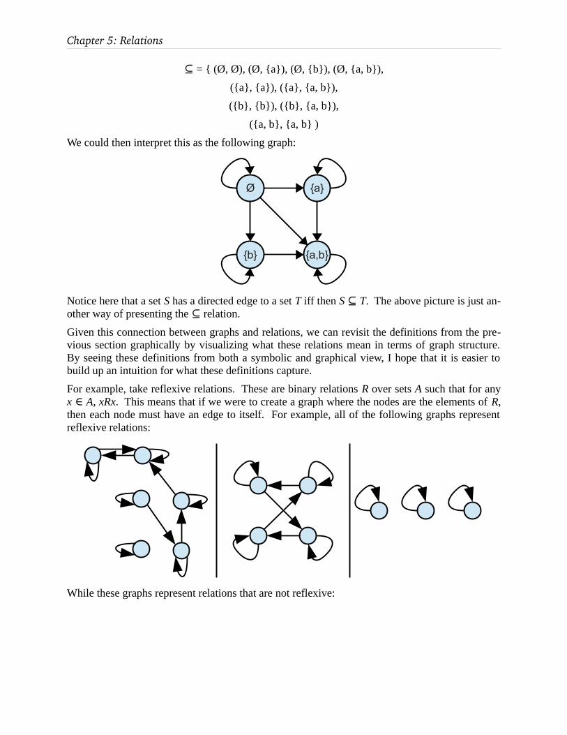
Chapter 5: Relations

= { (Ø, Ø), (Ø, {a}), (Ø, {b}), (Ø, {a, b}),⊆

({a}, {a}), ({a}, {a, b}),

({b}, {b}), ({b}, {a, b}),

({a, b}, {a, b} )

We could then interpret this as the following graph:

Ø {a}

{b} {a,b}

Notice here that a set S has a directed edge to a set T iff then S ⊆ T. The above picture is just an-other way of presenting the relation.⊆

Given this connection between graphs and relations, we can revisit the definitions from the pre-vious section graphically by visualizing what these relations mean in terms of graph structure. By seeing these definitions from both a symbolic and graphical view, I hope that it is easier to build up an intuition for what these definitions capture.

For example, take reflexive relations. These are binary relations R over sets A such that for any x ∈ A, xRx. This means that if we were to create a graph where the nodes are the elements of R, then each node must have an edge to itself. For example, all of the following graphs represent reflexive relations:

While these graphs represent relations that are not reflexive:

279 / 347

Take a minute to confirm why none of these relations are reflexive.

Similarly, a relation that is irreflexive (that is, for any x ∈ A, we know xRx) would be represented by a graph in which no node has an edge to itself. For example, all of the following graphs rep-resent irreflexive relations:

While none of the following graphs represent irreflexive relations:

Again, make sure you understand why none of these graphs represent irreflexive relations.

The next property of relations we explored was transitivity. If you'll recall, a binary relation R over a set A is called transitive iff for any x, y, z ∈ A, that if xRy and yRz, then xRz. What does this mean from a graph-theoretic perspective? Well, xRy means that there is an edge from x to y, and yRz means that there is an edge from y to z. Transitivity says that if we have these edges, then it must also be the case that xRz, meaning that there is an edge from x to z.

Chapter 5: Relations

This suggests an elegant, graph-theoretic intuition for transitivity. Suppose that you have three nodes x, y, and z. Transitivity says that if you can get from x to z by going from x to y and from y to z, then you can also get directly from x to z. This is shown below:

x

y

z

You can thus think of a transitive relation as one that guarantees that all paths can be “shortcut-ted.” If it's ever possible to get from one node to another along any path, there will always be a direct path from the first node to the destination.* As a result, these graphs all represent transitive relations:

One important detail about transitivity. Suppose that we have a pair of nodes like these, in which each node has an edge to the other:

x y

In this case, if the relation is transitive, there must be edges from each node to itself. To see why, note that from the above graph, we know that xRy and that yRx. By the definition of transitivity, this means that xRx. Similarly, since yRx and xRy, we are guaranteed that yRy. Consequently, both of the following graphs represent transitive relations:

* One of the chapter exercises asks you to formally prove this.

281 / 347

While none of these do:

As before, make sure you understand why the above graphs aren't transitive.

Finally, let's consider the last two properties of relations we introduced: symmetry and asymme-try. Recall that R is a symmetric relation over A iff whenever xRy, it's also the case that yRx. From a graph-theoretic perspective, this means that any time there is an edge from x to y, there must also be an edge back from y to x. In other words, for any pair of nodes x and y, either there are edges going between them in both directions, or there are no edges between them at all. Con-sequently, the following graphs all represent symmetric relations:

While these graphs do not:

Note that it's perfectly fine for a node to have an edge from itself. This represents xRx, which is acceptable in symmetric relations because it's true that if xRx, then after swapping x and x, we still get that xRx.

Chapter 5: Relations

The case of asymmetry is slightly different. In an asymmetric relation, if xRy, then yRx. This means that if there is an edge from x to y, then there cannot be an edge from y to x. In other words, if there is an edge from one node to another, there cannot be another edge going the other way. Consequently, for any pair of nodes, there are either zero or one edges between them.

Additionally, asymmetric relations cannot have any edges from a node to itself. The reasoning is the following: if xRx, then since R is asymmetric, we should have xRx, which is impossible. Consequently, no asymmetric relation has self-loops.

Given these descriptions, we have that the following graphs all represent asymmetric relations:

While these graphs do not:

5.2 Equivalence RelationsNow that we have some terminology we can use to describe relations, we will explore several important classes of relations that appear repeatedly throughout computer science and discrete mathematics.

The first type of relation that we will explore is the equivalence relation. Informally, an equiva-lence relation is a binary relation over some set that tells whether two objects have some essen-tial trait in common. For example, = is an equivalence relation that tells whether two objects are identically the same. The connectivity relation ↔ in a graph is an equivalence relation that tells whether two nodes are in the same connected component as one another. The relation “x is the same color as y” is an equivalence relation that tells whether two objects share a color.

If we take these three relations as exemplars of equivalence relations, you will notice that they all have three traits in common:

283 / 347

• Reflexivity. Every object has the same traits as itself. Thus our relation should be re-flexive.

• Symmetry. If x and y have some trait in common, then surely y and x have some trait in common.

• Transitivity. If x and y have some trait in common and y and z have the same trait in common, then x and z should have that same trait in common.

These three properties, taken together, are how we formally define equivalence relations:

A binary relation R over a set A is called an equivalence relation iff it is reflexive, sym-metric, and transitive.

Some of the relations that we have seen before are equivalence relations. For example, consider any undirected graph G = (V, E) and the connectivity relation ↔ on that graph. We proved in Chapter 5 that this relation is reflexive, symmetric, and transitive, though at the time we didn't actually use those names. Consequently, ↔ is an equivalence relation over nodes in graphs.

5.2.1 Equivalence ClassesAn important observation at this point is that while intuitively we want equivalence relations to capture the notion of “x and y have some trait in common,” our definition says absolutely noth-ing about this. Instead, it focuses purely on three observable traits of relations: reflexivity, sym-metry, and transitivity.

This definition might initially seem somewhat arbitrary. Why is this class of relations at all inter-esting? And why does this capture our idea of a relation indicating whether objects have traits in common?

One key property of equivalence relations is that we can use them to partition objects into dis-tinct groups, all of which share some key property. For example, given the equivalence relation “x is the same color as y,” we could break objects apart into groups of objects that all have the same color as one another. Given the equivalence relation x ↔ y, we could break nodes in a graph apart into groups of nodes that are all mutually connected to one another (those groups are the connected components of the graph; more on that later). Even if we take the somewhat silly equivalence relation x = y, we can still split objects into groups. We just end up partitioning all objects into groups of one object apiece.

To formalize this definition, let us introduce a few quick definitions. First, we need to define what it means to take some set S and split it apart into different groups. Intuitively, this means that we start out with all of the elements of S:

Chapter 5: Relations

Then cut them apart into smaller sets of elements:

When cutting the elements up into sets this way, there are two key properties that must hold. First, every element of the original set S must belong to one of the smaller sets. Second, no ele-ment of the original set S can belong to more than one of the smaller sets. In addition to these two key properties, we'll add one extra requirement. When cutting S up into smaller sets S1, S2, …, we'll require that each of these sets is nonempty. After all, we want to distribute the elements of S into a collection of smaller sets, and allowing one of these smaller sets to be empty doesn't really accomplish anything (it doesn't actually contain any of the elements of S).

These requirements are formalized in the following definition:

Given a set S, a partition of S is a set X (⊆ ℘ S) (that is, a set of subsets of S) with the fol-lowing properties:

1. The union of all sets in X is equal to S.2. For any S1, S2 ∈ X with S1 ≠ S2, we have that S1 ∩ S2 = Ø (S1 and S2 are disjoint)3. Ø ∉ X.

For example, let S = {1, 2, 3, 4, 5}. Then the following is a partition of S:

{ {1}, {2}, {3, 4}, {5} }

As is this set:

{ {1, 4}, {2, 3, 5} }

285 / 347

As is this set:

{ {1, 2, 3, 4, 5} }

However, the following set is not a partition of S:

{ {1, 3, 5}, {2} }

Because the union of these sets does not give back S. The following set isn't a partition either:

{ {1, 2, 3}, {4}, {3, 5} }

Because 3 is contained in two of these sets. Finally, this set isn't a partition of S:

{ {1, 2, 3}, {4, 5}, Ø }

Since it contains the empty set.

One important observation is that it is indeed possible to build a partition over the empty set. Specifically, Ø is a partition over Ø. You can check to see that Ø obeys all of the required prop-erties – the union of all the (nonexistent sets) in Ø is the empty set itself. There are no two dif -ferent sets in Ø, so vacuously all of the sets in Ø are disjoint. Finally, Ø Ø. Thus Ø is a parti∉ -tion of itself.

There is a close connection between partitions and equivalence relations, as you'll see, but in or-der to explore it we will need to explore a few quick properties of partitions. First, we'll prove a simple but important lemma that we'll need while reasoning about partitions:

Lemma: Let S be a set and X a partition of S. Then every element u ∈ S belongs to exactly one set Y ∈ X.

In other words, this lemma says that if you cut the elements of S apart into non-overlapping groups, every element of S belongs to just one of those groups. This is a key feature of parti-tions, so before we proceed onward, we'll prove this result.

Proof: Let S be a set and X a partition of S. We will show that every element u ∈ S be-longs to at least one set Y ∈ X and to at most one set Y ∈ X.

To see that every element u ∈ S belongs to at least one set Y ∈ X, note that since X is a par-tition of S, the union of all the sets in S must be equal to S. Consequently, there must be at least one set Y ∈ X such that u ∈ Y, since otherwise the union of all sets contained in X would not be equal to S.

To see that every element u ∈ S belongs to at most one set Y ∈ X, suppose for the sake of contradiction that u belongs to two sets Y1, Y2 ∈ X with Y1 ≠ Y2. But then x ∈ Y1 ∩ Y2, meaning that Y1 ∩ Y2 ≠ Ø, a contradiction. We have reached a contradiction, so our as-sumption must have been wrong.

Thus every element u ∈ S belongs to at most one set Y ∈ X. ■

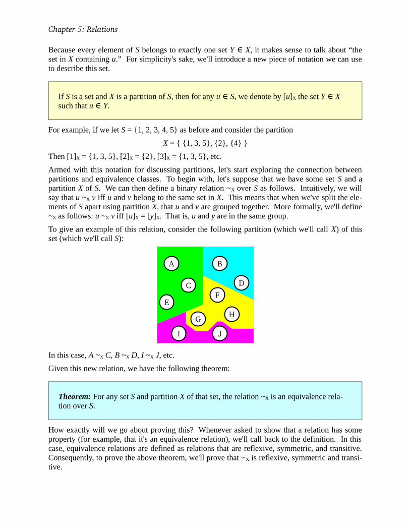
Chapter 5: Relations

Because every element of S belongs to exactly one set Y ∈ X, it makes sense to talk about “the set in X containing u.” For simplicity's sake, we'll introduce a new piece of notation we can use to describe this set.

If S is a set and X is a partition of S, then for any u ∈ S, we denote by [u]X the set Y ∈ X such that u ∈ Y.

For example, if we let S = {1, 2, 3, 4, 5} as before and consider the partition

X = { {1, 3, 5}, {2}, {4} }

Then [1]X = {1, 3, 5}, [2]X = {2}, [3]X = {1, 3, 5}, etc.

Armed with this notation for discussing partitions, let's start exploring the connection between partitions and equivalence classes. To begin with, let's suppose that we have some set S and a partition X of S. We can then define a binary relation ~X over S as follows. Intuitively, we will say that u ~X v iff u and v belong to the same set in X. This means that when we've split the ele-ments of S apart using partition X, that u and v are grouped together. More formally, we'll define ~X as follows: u ~X v iff [u]X = [y]X. That is, u and y are in the same group.

To give an example of this relation, consider the following partition (which we'll call X) of this set (which we'll call S):

A

F

G H

I

C

E

J

B

D

In this case, A ~X C, B ~X D, I ~X J, etc.

Given this new relation, we have the following theorem:

Theorem: For any set S and partition X of that set, the relation ~X is an equivalence rela-tion over S.

How exactly will we go about proving this? Whenever asked to show that a relation has some property (for example, that it's an equivalence relation), we'll call back to the definition. In this case, equivalence relations are defined as relations that are reflexive, symmetric, and transitive. Consequently, to prove the above theorem, we'll prove that ~X is reflexive, symmetric and transi-tive.

287 / 347

Intuitively, we can see that ~X has these three properties as follows:

• Reflexivity: We need to show that for any u ∈ S, that u ~X u. Calling back to the defini-tion of ~X, this means that we need to show that [u]X = [u]X, which is obvious.

• Symmetry: We need to show that for any u, v ∈ S that if u ~X v, then v ~X u. This means we need to show that if [u]X = [v]X, then [v]X = [u]X. Again, this is obviously true.

• Transitivity: We need to show that for any u, v, w ∈ S, that if u ~X v and v ~X w, then u ~X w. This means that if [u]X = [v]X and [v]X = [w]X, then [u]X = [w]X. This is also obvi-ously true by the transitivity of =.

We can formalize this proof below:

Theorem: For any set S and partition X of that set, the relation ~X is an equivalence relation over S.

Proof: We need to show that ~X is reflexive, symmetric, and transitive.

To see that ~X is reflexive, we need to prove that for any u ∈ S, that u ~X u. By definition, this means that we need to show that [u]X = [u]X, which is true because = is reflexive.

To see that ~X is symmetric, we need to show that if u ~X v, then v ~X u. By definition, this means that we need to show that if [u]X = [v]X, then [v]X = [u]X. This is true because = is symmetric.

To see that ~X is transitive, we need to show that if u ~X v and v ~X w, then u ~X w. By def-inition, this means that we need to show that if [u]X = [v]X and [v]X = [w]X, then [u]X = [w]X. This is true because = is transitive.

Since ~X is reflexive, symmetric, and transitive, it is an equivalence relation. ■

Great! We've just shown that if we start off with a partition, we can derive an equivalence rela-tion from it by saying that any pair of elements in the same group of the partition are equivalent.

It turns out that we can also go the other way as well: given any equivalence relation R over a set S, it's possible to construct a partition of S by grouping together all the objects that are related to-gether by R. To motivate this discussion, suppose that we have this collection of objects:

Chapter 5: Relations

If we group all of these objects together by the equivalence relation “x is the same color as y,” then we end up with this partition of the set of objects:

Similarly, if we group these objects together by the equivalence relation “x is the same shape as y,” we get this partition:

The key insight behind why equivalence relations induce a partition of the elements is that it makes sense, given any element u, to speak of “all the elements equal to u.” If you look at either of the above induced partitions, you can see that each set in the partition can be thought of as a set formed by picking any one of the elements in the set, then gathering together all the elements equal to it.

Given an equivalence relation R over a set A and some element x ∈ A, the equivalence class of x is the set of all elements of A that compare equal to A. This is formalized with the following def-inition:

Let R be an equivalence relation over a set A. Then for any x ∈ A, the equivalence class of x is the set { y ∈ A | xRy }. We denote this set [x]R.

289 / 347

When discussing equivalence classes, note that it's possible for two different elements of A to have the same equivalence class. For example, in the equivalence relation “x has the same color as y,” the equivalence classes for any two red objects will be the same. Also notice that we are using similar notations for equivalence classes of an equivalence relations and the set in a parti-tion containing some element. We will justify why this notation is so similar in the remainder of this section, but for now keep in mind that the notations do not necessarily represent the same thing.

Our goal in this section was to show how to turn an equivalence relation into a partition, and to do so we'll use equivalence classes. The key observation is as follows – if we have an equiva-lence relation R over a set A, we will take as our partition the set of all equivalence classes for all the elements of A. For example, if our equivalence relation is “x is the same color as y,” then we would take as our partition of all elements the set of all red objects, the set of all orange objects, the set of all yellow objects, etc. Therefore, in the rest of this section, we will prove that the set of all equivalence classes of R gives a partition of A.

First, some notational issues. How exactly do we define “the set of all equivalence classes of R?” To do this, we will consider this set:

X = { [x]R | x ∈ A }

This set is the set of the equivalence classes of every element in the set A. Notice that the rule we are using in the set-builder definition of X might multiply-count the same equivalence class multiple times. For example, if an equivalence class C contains three elements a, b, and c, then C will get included in X three times, since [a]R = [b]R = [c]R = C. However, this is not a problem. Remember that sets are unordered collections of distinct objects, so if we include some equiva-lence class multiple times in X, it's the same as if we included it only once.

Now that we have this set X, how do we prove that it is a partition of A? Well, let's look back at the definition of a partition. We'll need to prove three things:

1. The union of all sets in X is equal to A.

2. Any two non-equal sets in X are disjoint.

3. X does not contain the empty set.

Let's consider each of these in turn.

For starters, up to this point we've been using the term “the union of all sets in X” informally, without giving it a firm mathematical definition. If we want to reason about this union in the proof, we will need to actually define what this means.

In Chapter One, we defined the union of two sets as the set containing all elements in either of the original set. Let's generalize this definition to allow us to compute the union of any number of sets, even infinitely many.

For example, let's suppose that we have two sets A and B and want to their union. This is the union A ∪ B. In this case, we were computing the union of the sets contained within the set {A, B}. If we want to compute the union A ∪ B ∪ C, this would be computing the union of all the sets contained within the set {A, B, C}. More generally, if we have a set whose elements are other sets, we can take the union of all the sets contained within that set. This motivates the fol-lowing definition:

Chapter 5: Relations

Let S be a set whose elements are other sets. Then ∪S = { x | there is some X ∈ S such that x ∈ X }.

For example:

{ {1, 2, 3}, {3, 4} } = {1, 2, 3, 4}∪

{ Ø, {1}, {2}, {3} } = {1, 2, 3}∪

Ø = Ø∪

Given this new definition, let's start trying to prove that the set X = { [x]R | x ∈ A } is a partition of the set A. First, we need to prove that the union of all sets in X is equal to A. Using our new notation, this means that we want to prove that ∪X = A. Intuitively, this is true because we can show that every element of A belongs to its own equivalence class, which in turn is an element of X. We can formalize this reasoning below:

Lemma: Let R be an equivalence relation over A, and X = { [x]R | x ∈ A }. Then ∪X = A.

Proof: Let R be an equivalence relation over A, and X = { [x]R | x ∈ A }. We will prove that ∪X ⊆ A and A ⊆ ∪X, from which we can conclude that ∪X = A.

To show that ∪X ⊆ A, consider any x ∈ X. By definition of ∪X, since x ∈ X, this means that there is some [y]R ∈ X such that x [∈ y]R. By definition of [y]R, since x [∈ y]R, this means that yRx. Since R is a binary relation over A, this means that x ∈ A. Since our choice of x was arbitrary, this shows that if x ∈ ∪X, then x ∈ A. Thus ∪X ⊆ A.

To show that A ⊆ ∪X, consider any x ∈ A. We will prove that x [∈ x]R. If we can show this, then note that since x [∈ x]R and [x]R ∈ X, we have x ∈ X. Since our choice of x is ar-bitrary, this would mean that any x ∈ A satisfies x ∈ ∪X, so A ⊆ ∪X.

So let's now prove that x [∈ x]R. By definition, [x]R = { y ∈ A | xRy }. Since R is an equiv-alence relation, R is reflexive, so xRx. Consequently, x [∈ x]R, as required. ■

Great! We've established that ∪X = A, which is one of the three properties required for X to be a partition of A.

Notice that in the second half of this proof, we explicitly use the fact that x is reflexive in order to show that x [∈ x]R. A corollary of this result is that [x]R ≠ Ø for any x ∈ A. Consequently, we can also conclude that Ø ∉ X. Formally:

291 / 347

Lemma: Let R be an equivalence relation over A, and X = { [x]R | x ∈ A }. Then Ø ∉ X.

Proof: Using the logic of our previous proof, we have that for any x ∈ A, that x [∈ x]R. Consequently, for any x ∈ A, we know [x]R ≠ Ø. Thus Ø ∉ X. ■

All that is left to do now is to prove that any two sets [x]R, [y]R ∈ X with [x]R ≠ [y]R are disjoint. To see why this would be true, let's think intuitively about how equivalence classes work. The class [x]R is the set of all objects equal to x, and similarly [y]R is the set of all objects equal to y. If xRy, then we would have that [x]R = [y]R, since the objects equal to x are the same as the ob-jects equal to y. On the other hand, if xRy, then we should have that no object equal to x would compare equal to y.

To formally prove this result, we can proceed by contrapositive. We'll show that if the equiva-lence classes [x]R and [y]R are not disjoint, then they must be equal. Intuitively, the proof works as follows. Since [x]R ∩ [y]R ≠ Ø, there is some element w such that w [∈ x]R and w [∈ y]R. This means that xRw and yRw. From there, we can use symmetry and transitivity to get that xRy and yRx. Once we've done that, we can conclude, using transitivity, that everything equal to x is equal to y and vice-versa. Thus [x]R and [y]R must be equal.

We can formalize this here:

Lemma: Let R be an equivalence relation over A, and X = { [x]R | x ∈ A }. Then for any two sets [x]R, [y]R ∈ X, if [x]R ≠ [y]R, then [x]R ∩ [y]R = Ø.

Proof: Let R be an equivalence relation over A, and X = { [x]R | x ∈ A }. We proceed by contrapositive and show that for any [x]R, [y]R ∈ X, that if [x]R ∩ [y]R ≠ Ø, then [x]R = [y]R.

Consider any [x]R, [y]R ∈ X such that [x]R ∩ [y]R ≠ Ø. Then there must be some element w such that w [∈ x]R and w [∈ y]R. By definition, this means w { ∈ z ∈ A | xRz } and w { ∈ z ∈ A | yRz }. Consequently, xRw and yRw. Since R is symmetric, this means that xRw and wRy. Since R is transitive, this means that xRy. By symmetry, we also have that yRx.

We will now use this fact to show that [x]R [⊆ y]R. Without loss of generality, we can use this same argument to show that [y]R [⊆ x]R, from which we can conclude that [x]R = [y]R, as required.

To show that [x]R [⊆ y]R, consider any z [∈ x]R. This means that xRz. Since yRx and xRz, by transitivity we have that yRz. Consequently, z [∈ y]R. Since our choice of z was arbi-trary, we have that any z [∈ x]R satisfies z [∈ y]R. Thus [x]R [⊆ y]R, as required. ■

Notice that this theorem relies on the fact that equivalence relations are symmetric and transitive. If we didn't have that property, then we couldn't necessarily guarantee that we could link up the sets [x]R and [y]R as we did. In our earlier lemmas, we used the fact that equivalence relations are

Chapter 5: Relations

reflexive. Collectively, this gives some justification as to why we define equivalence relations this way. If a relation is indeed reflexive, symmetric, and transitive, then regardless of its other properties it has to induce a partition of the elements of the underlying set.

By combining the three earlier lemmas together, we get the following overall result:

Theorem: Let R be an equivalence relation over A, and let X = { [x]R | x ∈ A }. Then X is a partition of A.

The proof of this result is, essentially, “look at the previous three lemmas.” Accordingly, we don't gain much by writing it out formally.

If we have an equivalence relation R over a set A, then the set X described above (the set of all the equivalence classes of R) has a nice intuition – this is the set formed by grouping together all of the elements in A that are equal to one another. In other words, we divide the elements of the set A into groups based on the equivalence relation R. The fact that we are “dividing” elements up this way gives rise to the term we use for this set X: it's called the quotient set of A by R:

Let R be an equivalence relation over A. The quotient set of A by R is the set of all equiva-lence classes of the elements of A under R; that is, { [x]R | x ∈ A }. This set is denoted A / R.

For example, consider the set . One equivalence relation we can define over is the relationℕ ℕ “x has the same parity as y,” which is denoted ≡2. (There's a good reason for this notation; see the exercises for more details). For example, 5 ≡2 3, and 0 ≡2 100. In this case, there are two equivalence classes: the equivalence class containing the even numbers 0, 2, 4, 6, 8, …, and the equivalence class containing the odd numbers 1, 3, 5, 7, 9, … . Consequently, the set / ≡ℕ 2

would be the set { { 2n | n }, { 2∈ ℕ n + 1 | n } }.∈ ℕ

5.2.2 Equivalence Classes and Graph ConnectivityThe fact that equivalence relations induce a partition of the underlying set has numerous applica-tions in mathematics. In fact, we can use this general result we've just proven to obtain an alter-native proof of some of the results from Chapter Four.

If you'll recall, given an undirected graph G = (V, E), a connected component of G is a set of nodes C such that

• If x, y ∈ C, then x and y are connected (x ↔ y).

• If x ∈ C and y ∈ V – C, then x and y are not connected (x ↮ y)

We proved in the previous chapter that every node in a graph belongs to a unique connected component in that graph. To prove this, we proceeded by proving first that every node in the graph belongs to at least one connected component, then that each node in the graph belongs to

293 / 347

at most one connected component. However, now that we have started exploring equivalence re-lations, it's possible for us to prove this result as a special case of what we proved in the previous section on partitions.

Remember that the connectivity relationship ↔ is an equivalence relation; it's reflexive, symmet-ric, and transitive. Consequently, we know that we can derive a partition X = { [v]↔ | v ∈ V } of the nodes in G into equivalence classes based on the ↔ relationship. What exactly does this par-tition look like? Well, let's start by thinking about what an equivalence class [v]↔ looks like. This is the set {u ∈ V | v ↔ u} of all of the nodes in the graph that are connected to u. In other words, the set [v]↔ is the connected component containing v! Since we know that X is a partition of the nodes in G, this immediately tells us that every node belongs to a unique equivalence class. Since the equivalence classes of ↔ are the same as the connected components of G, this means that every node in G belongs to a unique connected component. And we're done!

5.3 Order RelationsIn the previous section, we explored equivalence relations, which let us group together objects that share some common property. In this section, we will explore several types of relations (col-lectively referred to as order relations) that allow us to rank different objects against one another. These relations will allow us to say that some objects are “greater” or “less” than others, to de -cide what objects are “better” or “worse” than one another, etc.

5.3.1 Strict OrdersOften, we will want to take a set of objects A and rank them against one another (for example, we might want to rank movies, restaurants, etc.) To do this, we might think about defining a bi-nary relation R over the set A, where xRy means “x is not as good as y,” for some definition of “goodness.” For instance, we could take the relation < over , where ℕ x < y means “x is smaller than y.” Taking a cue from Chapter Four, we could also define the relation “x is not as tasty as y,” giving an ordering over different types of food. We could even think about defining the rela-tion “x is smaller than y” over different buildings. Relations that rank objects this way are called strict orders, and in this section we will define them and explore their properties.

As with equivalence relations, our goal in this section will be to abstract away from concrete def-initions of strict orders and to try to find a small number of properties that must be held by a rela-tion in order for it to qualify as a strict order. Let's begin by thinking about what these properties might be.

To begin with, if we are ranking objects against one another with relations like “x < y” or “x is smaller than y,” how do individual objects compare to themselves? Well, we will never have that x < x for any choice of x, and no building is smaller than itself. More generally, no object will ever be strictly worse/smaller than itself. Consequently, all of these relations will be irreflexive.

These relations also have a few other interesting properties. For instance, let's suppose that x < y and y < z. From this, we can conclude that x < z. Similarly, if x runs faster than y and y runs faster than z, then x runs faster than z. More generally, if we are ranking objects against one an-other, we will usually find that the ranking is transitive. This isn't always the case – think about the game “Rock, Paper, Scissors,” in which Rock beats Scissors, Scissors beats Paper, and Paper beats Rock – but most rankings that we will encounter are indeed transitive.

Chapter 5: Relations

Finally, and perhaps most importantly, we will never find a pair of objects that are mutually “bet-ter” than one another. For example, if x < y, we can guarantee that y < x. Similarly, if x runs faster than y, we know for certain that y does not run faster than x. In other words, these rela-tions are asymmetric.

It turns out that these three properties capture the essential properties of relations that rank ob-jects. Irreflexivity guarantees that no object is less than itself. Asymmetry ensures that two ob-jects can't mutually rank higher than one another. Transitivity ensures that the ranking is consis-tent across all of the objects. Consequently, we use these three properties to formally define a strict order:

A binary relation R over a set A is called a strict order iff R is irreflexive, asymmetric, and transitive.

Given this definition, let's revisit some of the relations we've seen before to see which of them are strict orders. To begin with, let's look back at some of the operations that we have seen on sets. For example, let's take the binary relation over the set ( )⊆ ℕ℘ * (that is, the “is a subset of relation” over all sets of natural numbers). Is this relation a strict order? Well, to check this, we need to see if is irreflexive, asymmetric, and transitive.⊆

Of these three properties, we already know that is transitive (this was given as an exercise in⊆ Chapter Two; if you haven't proven this yet, take a minute to do so). Is asymmetric? With a⊆ few examples, it might seem to be the case; after all:

{cat, dog} {cat, dog, dikdik}, but not the other way around.⊆

Ø {1, 2, 3}, but not the other way around.⊆

, but not the other way around.ℕ ⊆ ℝ

However, is not actually asymmetric. Recall that every set is a subset of itself. This means⊆ that A ⊆ A. Asymmetry means that if A ⊆ A holds, then after swapping A and A, we should get that A ⊆ A is false. This, of course, isn't true. Consequently, isn't asymmetric. This same line⊆ of reasoning means that isn't irreflexive either, since ⊆ A ⊆ A is always true. As a result, is⊆ not a strict order.

It seems like the only reason that isn't a strict order is that it's possible for a set to be a subset⊆ of itself. What happens if we disallow this? In that case, we get the relation, the “strict sub⊂ -set” relation. As a refresher, we defined x ⊂ y to mean “x ⊆ y, and x ≠ y.” Let's look at this rela-tion. Is it a strict order?

As before, let's see whether it's irreflexive, asymmetric, and transitive. First, is irreflexive?⊂ This means that there is no set A such that A ⊂ A holds. We can see that this is true, since if A ⊂ A were true, it would mean A ≠ A, which is impossible. Second, is asymmetric? That⊂

* You might be wondering why we consider   over the set  ( ) and not, say, the set of all sets.  It turns ⊆ ℘ ℕout that “the set of all sets” is a mathematically troublesome object.  Some definitions of sets says that this set doesn't actually exist, while other definitions of sets allow the set of all sets, but only with very strict restrictions on how it can be used.  We'll sidestep this by defining   only over sets of naturals.⊆

295 / 347

would mean that whenever A ⊂ B, we know that B ⊂ A does not hold. Well, what would happen if we had both A ⊂ B and B ⊂ A? That would mean (by definition) that A ⊆ B, B ⊆ A, but A ≠ B. This can't happen, because if A ⊆ B and B ⊆ A, then A = B. We proved this in Chapter

Finally, is transitive? That is, if ⊂ A ⊂ B and B ⊂ C, does A ⊂ C? If we expand out the defini-tions, we are asking whether, given that A ⊆ B, B ⊆ C, A ≠ B, and B ≠ C, we can determine whether A ⊆ C and A ≠ C. Of these two properties, one is easy to establish – since is transi⊆ -tive, we know that A ⊆ C must be true. So how about A ≠ C? One way we can show this is by contradiction. Suppose, hypothetically, that A = C. Since B ⊂ C and C = A, this means that B ⊂ A. But that's impossible, since we know that A ⊂ B and we just proved that is asymmet⊂ -ric. Something is wrong here, so our initial assumption that A = C must have been wrong.

We can formalize the above intuition with the following proof:

Theorem: The relation over ( ) is a strict order.⊂ ℕ℘

Proof: We show that is irreflexive, asymmetric, and transitive.⊂

To show that is irreflexive, we must show that for any ⊂ A ( ) that ∈ ℕ℘ A ⊂ A does not hold. To see this, assume for the sake of contradiction that this is false and that there exists some A ( ) such that ∈ ℕ℘ A ⊂ A. By definition of , this means that ⊂ A ⊆ A and A ≠ A. But A ≠ A is impossible, since = is reflexive. We have reached a contradiction, so our as-sumption must have been wrong. Thus is reflexive.⊂

To show that is asymmetric, we must show that for any ⊂ A, B ( ) that if ∈ ℕ℘ A ⊂ B, then it is not the case that B ⊂ A. We proceed by contradiction; assume that this statement is false and that there exist some sets A, B ( ) such that ∈ ℕ℘ A ⊂ B and B ⊂ A. By defini-tion of , this means that ⊂ A ⊆ B, B ⊆ A, but A ≠ B. Since A ⊆ B and B ⊆ A, we know that A = B, contradicting the fact that A ≠ B. We have reached a contradiction, so our as-sumption must have been wrong. Thus is asymmetric.⊂

To show that is transitive, we need to show that for any ⊂ A, B, C ( ), that if ∈ ℕ℘ A ⊂ B and B ⊂ C, then A ⊂ C. Consider any A, B, C ( ) where ∈ ℕ℘ A ⊂ B and B ⊂ C. By defi-nition of , this means that ⊂ A ⊆ B, B ⊆ C, A ≠ B, and B ≠ C. We will show that A ⊂ C, meaning that A ⊆ C and A ≠ C. Since A ⊆ B and B ⊆ C, we know that A ⊆ C. To show that A ≠ C, assume for the sake of contradiction that A = C. Since B ⊂ C and C = A, this means that B ⊂ A. But this is impossible, because we also know that A ⊂ B, and is ⊂asymmetric. We have reached a contradiction, so our assumption must have been wrong. Thus A ≠ C. Since A ⊆ C and A ≠ C, this means that A ⊂ C as required.

Since is irreflexive, asymmetric, and transitive, it is a strict order over ( ). ■⊂ ℕ℘

Chapter 5: Relations

Before we conclude this section, there is one last detail we should explore. We just proved that is a strict order over sets of natural numbers. Notice, however, that not all sets of natural num⊂ -

bers can even be compared by . For example, if we take ⊂ A = {1, 2, 3} and B = {3, 4, 5}, then neither A ⊂ B nor B ⊂ A is true. If we are trying to use to rank different sets, we will find that⊂ neither A nor B would be considered “greater” or “lesser” than the other.

Many other strict orders cannot be used to establish a total ranking of the elements of the under-lying set. For example, consider the relation “x is tastier than y” over different types of food. In the previous chapter, I drew a DAG of my own personal food preferences, which looked like this:

Indian Mediterranean

Mexican

Italian

American Fast Food

Dorm Food

Notice that Indian and Mediterranean cuisine are incomparable. I really like both of them a lot, but I wouldn't say that one of them was necessarily better than the other. They're both really, re-ally good. However, I would say with certainty that they are much better than dorm food!

Both of the and “tastier than” relations are strict orders, but neither one of them is guaranteed⊂ to rank all elements of the underlying set against one another. On the other hand, some strict or-ders can rank all objects against one another. For example, the < relation over guarantees thatℕ if we pick any x, y with ∈ ℕ x ≠ y, we will find either that x < y or y < x. This suggests that the label “strict order” actually encompasses several different types of order relations. Some, like ⊂ and “tastier than” rank their elements, but might have many elements incomparable with one an-other. Others, like <, rank all underlying elements. To distinguish between the two, we will in-troduce two new definitions. First, we will need a way of formalizing the idea that any two dis-tinct elements are comparable. This is called trichotomy:

A binary relation R over a set A is called trichotomous iff for any x, y ∈ A, exactly one of the following holds: xRy, or yRx, or x = y.

Calling back to the graphical intuition for binary relations, a trichotomous relation is one where, for any pair of objects, there is exactly one edge running between them. For example, the fol-lowing relations are trichotomous:

297 / 347

While the following are not:

Given this new definition, we can formally make a distinction between strict orders that can rank all elements against one another versus strict orders that cannot.

A binary relation R over a set A is called a strict total order iff R is a strict order and R is trichotomous.

Strict total orders induce a linear ranking on their elements. We can, in theory, line up all of the elements of a set ordered by a strict total order in a way where if xRy, then x appears to the left of y. For example, if we do this to the natural numbers ordered by <, we get the normal ordering of the naturals:

0, 1, 2, 3, 4, 5, 6, 7, 8, 9, 10, 11, 12, …

To summarize this section: strict orders are orders like <, , or “tastier than” that allow us to⊂ rank objects against one another. Strict total orders are orders like < that completely rank the ele-ments of the underlying set.

5.3.2 Partial OrdersIn the previous section, we explored strict orders. These relations are called “strict” orders be-cause the relation usually has the form “x is strictly less than y,” “x is strictly better than y,” “x is a strict subset of y,” etc. Such orders give us a way to talk about relations like <, , etc. How⊂ -ever, strict orders don't give us a nice way to talk about relations like ≤ or , which still rank ob⊆ -jects against one another, but are slightly more forgiving than < or . Whereas the relation < is⊂

Chapter 5: Relations

“x is strictly less than y,” the relation ≤ is “x is not greater than y.” Whereas “x is taller than y” is a strict order, we could also consider the relation “x is not smaller than y,” which can also be used to rank elements.

Relations like ≤ and are called ⊆ partial orders. They order the elements of a set, just as strict orders do, but do so by saying that objects are “no bigger than” other objects, rather than objects are “smaller than” other objects.

As with equivalence relations and strict orders, we will define partial orders by looking for prop-erties shared by all partial orders, then distilling the definition down to those key traits. Consid-ering that partial orders are in a sense a “softer” version of strict orders, it might be useful to see what properties of strict orders carry over to partial orders. If you'll recall, the three properties required of strict orders are irreflexivity, asymmetry, and transitivity. How many of these proper-ties still hold for relations like ≤, , and “⊆ x is no taller than y?”

Immediately, we can see that none of these relations are irreflexive. Any number x satisfies x ≤ x, any set A satisfies A ⊆ A, and any building b satisfies “b is no taller than b.” While strict orders are irreflexive, partial orders are all reflexive, since every object should be no greater than itself, no less than itself, no bigger than itself, no greener than itself, etc.

How about asymmetry? Here, the picture is more complicated. While in many cases ≤ acts asymmetrically (for example, 42 ≤ 137, but it is not the case that 137 ≤ 42), the relation ≤ is not asymmetric. Take, for example, 137 ≤ 137, which is true. If ≤ were asymmetric, we would have to have that, since 137 ≤ 137 is true, then after exchanging the order of the values, we should have that 137 ≤ 137 does not hold. Of course, 137 ≤ 137 does hold. This single counterexample means that ≤ is not an asymmetric relation. This same reasoning lets us see that is not asym⊆ -metric, because any set is a subset of itself, and that “x is no taller than y” is not asymmetric ei-ther.

That said, these relations are “mostly” asymmetric. If we pick any x ≠ y, then if x ≤ y, we're guaranteed that y ≤ x won't be true. Similarly, if A ≠ B and A ⊆ B, then we can be sure that B ⊆ A isn't true. In a sense, these relations are mostly asymmetric, in that they behave like asymmetric relations as long as the two objects being compared aren't identically the same. Re-lations with this property are extremely common, and so we give a name to this property: anti-

A binary relation R over a set A is called antisymmetric iff for any x, y ∈ A, if x ≠ y, then if xRy, we have yRx.

Equivalently, a binary relation R over a set A is antisymmetric iff for any x, y ∈ A, if xRy and yRx, then x = y.

I've listed two different ways of defining antisymmetry above. The first definition more closely matches the intuition we built in the above section – namely, a relation is antisymmetric if for any pair of unequal values, the relation acts asymmetrically. The second definition is a different way of thinking about this property. It says that if you can find two objects that each are no greater than one another, we can guarantee that those objects must be one and the same. For ex-

299 / 347

ample, if x ≤ y and y ≤ x, it's safe to conclude that x = y. Similarly, if A ⊆ B and B ⊆ A, then A = B. At times, one of these definitions will be easier to work with than the other, so it's good to know both of these definitions.

Graphically, what does an antisymmetric relation look like? In many ways, it's similar to an asymmetric relationship. If you pick any pair of distinct nodes in the graph, there can be at most one edge between them. However, unlike an asymmetric relation, it's fine for there to be edges from nodes to themselves. This would indicate, for example, something like “x is no bigger than itself.” Below are some examples of antisymmetric relations:

An important detail – just as symmetry and asymmetry are not opposites of one another, symme-try and antisymmetry are not opposites, or are asymmetry and antisymmetry. In fact, every asymmetric relation is also antisymmetric, and (as you'll see in the chapter exercises) it's possible for a relation to be symmetric and antisymmetric at the same time. If you want to prove that a relation is antisymmetric, you will need to explicitly prove that it satisfies the definition given above.

Great! At this point, we've seen that the three relations we've picked as representatives of partial orders are both reflexive and antisymmetric. There is one last property that we haven't yet inves-tigated – transitivity. As we saw when discussing strict orders, all strict orders are transitive. Does the same hold true for partial orders? All three of the sample partial orders we've seen end up being transitive:

If x ≤ y and y ≤ z, then x ≤ z.

If A ⊆ B and B ⊆ C, then A ⊆ C.

If x is no taller than y and y is no taller than z, then x is no taller than z.

More generally, transitivity is an important property that we want to have of partial orders. Just as with strict orders, we want to ensure that our rankings are consistent across objects.

The three traits we've identified – reflexivity, antisymmetry, and transitivity – end up being the essential traits of partial orders, and in fact this is how we will define them.

A binary relation R over a set A is called a partial order iff R is reflexive, antisymmetric, and transitive.

Chapter 5: Relations

Partial orders are extremely common in discrete mathematics and computer science. It is very common to speak of “partially ordered sets,” sets with an associated partial order. In fact, this terminology is so important that we should draw a light yellow box around it:

A partially ordered set (or poset) is a pair (A, R) where A is a set and R is a partial order over A.

Partial orders and strict orders collectively are called order relations:

A binary relation R over a set A is called an order relation iff R is a partial order or R is a strict order.

Although partial and strict orders have different properties, they behave similarly in many con-texts. As a result, most of the results from the latter part of this chapter that deal with partial or-ders or strict orders will work with either type of order interchangably. Consequently, we will discuss properties of order relations in general, mentioning specifically that we are working with partial or strict orders only in the case where a certain property applies to only one type of order.

To give a more elaborate example of a partial order, let's consider the divides relation |. Recall that we write m | n to mean “m divides n.” When we restrict ourselves to talking about the natu-ral numbers, we formally defined the | relation as follows: m | n iff there exists some q such∈ ℕ that n = mq. It turns out that this relation defines a partial order over the set . To formallyℕ prove this, we will need to show that | is reflexive, antisymmetric, and transitive. Let's consider each in turn.

First, we need to show that | is reflexive, meaning that for any n , that ∈ ℕ n | n. Intuitively, it should be clear that every number divides itself. Formally, we can show this by noting that n = 1 · n, meaning that there is some choice of q (namely, 1) where n = qn.

Next, we need to show that | is antisymmetric over . This is a bit trickier than it might seem.ℕ If we don't restrict ourselves to natural numbers and instead consider divisibility over the set of all integers , then | is ℤ not antisymmetric. For example, -2 | 2 and 2 | -2, but 2 ≠ -2. In order to show that | is antisymmetric, we're going to need to be clever with how we structure our argu-ment.

The approach we will take is the following. Let's suppose that m, n , that ∈ ℕ m ≠ n, and that m | n. This means that there is some q such that ∈ ℕ n = mq. We want to show that n | m is false, meaning that there is no r such that m = nr. To do this, let's see what happens if such an r were to exist. Since n = mq and m = nr, we get that

n = mq = (nr)q = nrq

m = nr = (mq)r = mrq

301 / 347

So n = nqr and m = mqr. Now, we know that m and n cannot simultaneously be zero, because m ≠ n. So that means that for at least one of these equalities, we can divide through by m or n safely, getting tha 1 = qr. Since q and r are natural numbers, the only way that this is possible is if q = r = 1. But if this happens, then n = mq = m, meaning that m = n, a contradiction.

This is a fairly long-winded argument, but such is the nature of this proof. What we are doing is very specific to the fact that we're working with natural numbers and how we have defined divis-ibility. As an exercise, try looking over this proof and see what goes wrong if we now allow m and n to be integers rather than natural numbers.

We've established that, over , | is reflexive and antisymmetric. So how do we show that it'sℕ transitive? Well, suppose that m | n and n | p. This means that there exists natural numbers q and r such that n = mq and p = rn. Combining these, we get that p = qrm = (qr)m. Thus there is some natural number k, namely qr, such that p = km. Therefore m | p.

We can formalize this reasoning in the following proof:

Theorem: | is a partial order over .ℕ

Proof: We will show that | is reflexive, antisymmetric, and transitive. To see that | is re-flexive, we will prove that for any n , that ∈ ℕ n | n (that there exists some q such that∈ ℕ n = nq). So let n be any natural number, and take q = 1. Then nq = n · 1 = n, so n | n.

To see that | is antisymmetric, we will prove that for any m, n , that if ∈ ℕ m | n and n | m, that m = n. Consider any m, n where ∈ ℕ m | n and n | m. This means that there exists q, r such that ∈ ℕ n = mq and m = nr. Consequently:

m = nr = (mq)r = mqrn = mq = (nr)q = nqr

We now consider two cases. First, if m = n = 0, then we are done, since m = n. Otherwise, at least one of m or n is nonzero; without loss of generality, assume m ≠ 0. Then since m = mqr, we know that 1 = qr. Since q, r , this is only possible if ∈ ℕ q = r = 1. Conse-quently, we have that m = nr = n · 1 = n, so m = n, as required.

To see that | is transitive, we will prove that for any m, n, p , that if ∈ ℕ m | n and n | p, then m | p. Consider any m, n, p where ∈ ℕ m | n and n | p; then there must exist q, r ∈ ℕsuch that n = qm and p = rn. Consequently, p = rn = r(qm) = qrm = (qr)m. Since qr ∈ , this means that there is some ℕ k (namely, ∈ ℕ qr) such that p = km. Thus m | p, as required.

Since | is reflexive, antisymmetric, and transitive over , | is a partial order over .ℕ ℕ

Chapter 5: Relations

To round out this section, let us draw one further parallel with strict orders. If you'll recall, we noted that some strict orders, like <, could be used to rank any arbitrary pair of values. Other strict orders, like , could not necessarily rank all values against one another. This led us to⊂ draw a distinction between strict orders and strict total orders.

This same distinction exists when discussing partial orders. For example, ≤, when applied to real or rational numbers, can rank any pair of values. However, | cannot; for example, both 3 | 5 and 5 | 3 are false. This motivates a refinement of partial orders into two subgroups - “plain old” par-tial orders, which are just reflexive, symmetric, and transitive, and “total” partial orders that can always rank elements against one another.

To do this, we will introduce one more definition:

A binary relation R over a set A is called total iff for any x, y ∈ A, at least one of xRy and yRx is true.

In other words, a total order is one in which any pair of values is guaranteed to be related some-how. Graphically, total relations are relations where any pair of nodes necessarily must have an edge between them. Additionally, in a total relation, all nodes must have edges to themselves, since by the above definition xRx has to hold for all x ∈ A. Consequently, the following graphs represent total relations:

Given this definition, we can now differentiate between partial orders and a stronger class of or-dering relations called total orders:

A binary relation R over a set A is called a total order iff R is total and R is a partial order.

Total orders (or strict total orders) are the types of relations you would want to use when trying to sort a list of values. They guarantee that there is a “correct” way to sort the list – put the least value first, then the next biggest, then the next biggest, etc. This is only possible if we have a (strict) total order over the elements, since otherwise we might have a situation in which no one value is smallest or largest. The chapter exercises ask you to play around with this to verify why it is correct.

303 / 347

5.3.3 Hasse DiagramsThroughout this chapter, we've intermittently switched to a graphical view of relations to high-light some of the important properties of different types of relations. We have just finished dis-cussing strict orders and partial orders, but haven't yet visualized what they look like. This sec-tion explores how to draw strict and partial orders.

Let's begin with a simple partial order: the relation defined over ({1, 2, 3}). This is the sub⊆ ℘ -set relation over sets containing the elements 1, 2, and 3. If we draw out the graph of this rela -tion, we get the following:

{1, 2, 3} {1, 2} {1, 3}

{2, 3} {1} {2}

{3} Ø

Yikes! That's almost impossible to read! Is there some way that we might simplify this?

First, let's return to our original intuition about partial orders. We started exploring these rela-tions in order to be able to rank elements in some set against one another. Accordingly, let's try redrawing that above graph so that we put “bigger” elements up at the top and “smaller” ele-ments down at the bottom. If we do that, we get this picture:

{1, 2, 3}

{1, 2} {1, 3} {2, 3}

{1} {2} {3}

Ø

Chapter 5: Relations

This is slightly easier to read than before, but it's still pretty crowded. For starters, note that ev-ery node in this graph has a loop to itself. This is because , like all partial orders, is reflexive,⊆ and graphs of reflexive relations always have every node containing an edge to itself. Of course, all partial orders are reflexive. If we are trying to draw out a partial order, we could save some time and effort by simply omitting these self-loops. We know that they're supposed to be there, but adding in those self-loops just makes the drawing a bit harder to read. If we eliminate those loops, we get this drawing, which is slightly easier to read than before:

{1, 2, 3}

{1, 2} {1, 3} {2, 3}

{1} {2} {3}

Ø

Let's see if we can further simplify this picture. Notice right now that all of the edges we've drawn are directed edges. This makes sense, since we want to be able to tell, for any pair of val -ues, which value (if any) is less than the other. However, remember that is antisymmetric.⊆ This means that if we have any two distinct values, we can't ever have edges running between them in opposite directions; there will either be an edge running in one direction, or no edges at all. Since we've drawn this picture by putting larger elements up at the top and smaller elements at the bottom, we can erase all of the arrows from this picture without encountering any prob-lems. We'll just implicitly assume that the arrows always point upward. This means that we don't need to draw out lots of clunky arrowheads everywhere. If we do this, we get the following picture:

{1, 2, 3}

{1, 2} {1, 3} {2, 3}

{1} {2} {3}

Ø

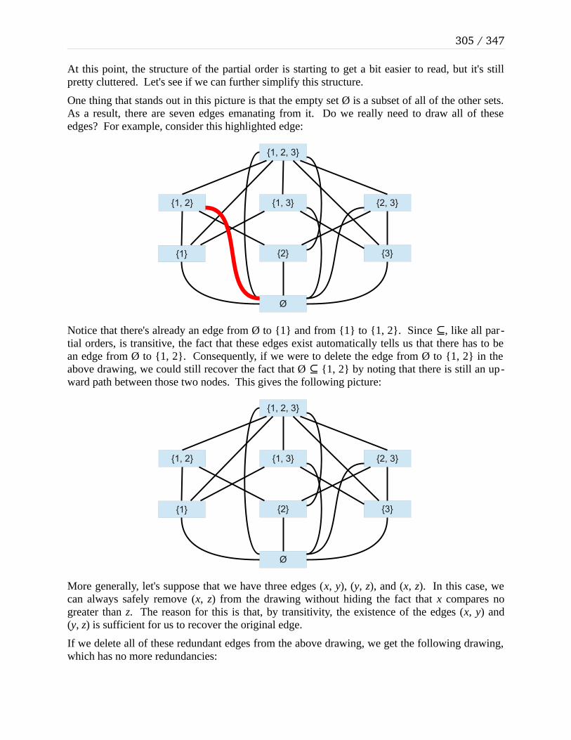
305 / 347

At this point, the structure of the partial order is starting to get a bit easier to read, but it's still pretty cluttered. Let's see if we can further simplify this structure.

One thing that stands out in this picture is that the empty set Ø is a subset of all of the other sets. As a result, there are seven edges emanating from it. Do we really need to draw all of these edges? For example, consider this highlighted edge:

{1, 2, 3}

{1, 2} {1, 3} {2, 3}

{1} {2} {3}

Ø

Notice that there's already an edge from Ø to {1} and from {1} to {1, 2}. Since , like all par⊆ -tial orders, is transitive, the fact that these edges exist automatically tells us that there has to be an edge from Ø to {1, 2}. Consequently, if we were to delete the edge from Ø to {1, 2} in the above drawing, we could still recover the fact that Ø {1, 2} by noting that there is still an up⊆ -ward path between those two nodes. This gives the following picture:

{1, 2, 3}

{1, 2} {1, 3} {2, 3}

{1} {2} {3}

Ø

More generally, let's suppose that we have three edges (x, y), (y, z), and (x, z). In this case, we can always safely remove (x, z) from the drawing without hiding the fact that x compares no greater than z. The reason for this is that, by transitivity, the existence of the edges (x, y) and (y, z) is sufficient for us to recover the original edge.

If we delete all of these redundant edges from the above drawing, we get the following drawing, which has no more redundancies:

Chapter 5: Relations

{1, 2, 3}

{1, 2} {1, 3} {2, 3}

{1} {2} {3}

Ø

This drawing is the cleanest way of representing the relation over these sets. We have used⊆ our knowledge that is reflexive to eliminate self-loops, that is antisymmetic to eliminate the⊆ ⊆ arrowheads, and that is transitive to eliminate extraneous edges. Given just this graph, we can⊆ present all of the information necessary to understand in a compact, readable form.⊆

Interestingly, we could have also drawn out a schematic of the strict order this way. Since ⊂ ⊂ is irreflexive, we'd have no self-loops to eliminate in the first place. Since is asymmetric, we⊂ could similarly eliminate the directions of the arrows and implicitly assume that they're directed upward. Since is transitive, we could still eliminate redundant edges in the graph.⊂

The diagram we have just made is our first example of a Hasse diagram, a graphical representa-tion of an order relation. Formally, a Hasse diagram is defined as follows:

Given a strict or partial order relation R over a set A, a Hasse diagram for R is a drawing of the elements of A with the following properties:

1. All edges are undirected.2. If there is an edge from x to y and x is below y in the diagram, then xRy.3. There are no self-loops.4. There are no redundant edges: if there is an edge from x to y and an edge from

y to z, then there is no edge from x to z.

For example, here is a Hasse diagram for the < relation over the set {1, 2, 3, 4}:

4

3

2

1

307 / 347

And here's a Hasse diagram for | over the natural numbers between 1 and 12:

4

3 2

1

8

5

6

12

9 10

7

If we look at these Hasse diagrams, we can start to notice certain differences between the struc-tures of these order relations. For example, look at the Hasse diagram for . If you'll notice, the⊆ set {1, 2, 3} is clearly the “biggest” element, while Ø is clearly the “smallest.” Similarly, in the diagram for <, 1 is clearly the “smallest” element, while 4 is clearly the “biggest.” On the other hand, if we look at the Hasse diagram for divisibility over the numbers between 1 and 12, there is no clear “biggest” or “smallest” elements. For example, 8, 9, 10, 11, and 12 aren't connected to anything above them, but no single one of them is the “biggest” value in that every other value in the set divides it. However, the value 1 is indeed the “smallest” value here.

To formalize our terminology, let's formally specify what's meant by “biggest” and “smallest” values.

Let R be a partial order over A. An element x ∈ A is called the greatest element of A iff for all y ∈ A, yRx. An element x ∈ A is called the least element of A iff for all y ∈ A, xRy.

Let R be a strict order over A. An element x ∈ A is called the greatest element of A iff for all y ∈ A where y ≠ x, yRx. An element x ∈ A is called the least element of A iff for all y ∈ A where y ≠ x, xRy.

For example, Ø is the least element of the partial order defined by over ({1, 2, 3}), while⊆ ℘ {1, 2, 3} is the greatest. There is no greatest element of the naturals between 1 and 15 when or-dered by divisibility, but 1 is the least element.

An important observation is that greatest and least elements of some ordered set A, if they even exist, are guaranteed to be unique. That is, no set can have two greatest elements or two least el-ements. We can prove this below for partially-ordered sets; the proof for strictly-ordered sets is similar and is left as an exercise.

Theorem: Let R be a partial order over set A. Then if R contains a greatest element, it con-tains exactly one greatest element.

Chapter 5: Relations

Proof: Let R be a partial order over A, and assume that g ∈ A is the greatest element of A. We will show that there are no other greatest elements of A. To do so, we proceed by con-tradiction; assume that there is some other greatest element h ∈ A with g ≠ h. Since g is a greatest element of A, we have that hRg. Since h is a greatest element of A, we have that gRh. Since R is a partial order, it is antisymmetric, and so g = h. This contradicts the fact that g ≠ h. We have reached a contradiction, so our assumption must have been wrong. Thus if A has a greatest element, it has a unique greatest element. ■

The fact that there is a unique greatest element (if one even exists in the first place) allows us to talk about the greatest element of an ordered set, rather than just a greatest element. We can sim-ilarly speak about the least element, rather than a least element.

We can generalize our discussion of greatest and least elements in an entire set to greatest and least elements of subsets of that set. For example, although the naturals between 1 and 15 don't have a greatest element, if we look at just the subset {1, 2, 3, 4, 6, 12}, then there is a greatest el -ement, namely 12. Consequently, let's extend our definitions from before to let them work with any collection of values from an ordered set:

Let R be a partial order over A and S ⊆ A be a set of elements from A. An element x ∈ S is called the greatest element of S iff for all y ∈ S, yRx. An element x ∈ S is called the least element of S iff for all y ∈ S, xRy.

Let R be a strict order over A and S ⊆ A be a set of elements from A. An element x ∈ S is called the greatest element of A iff for all y ∈ S where y ≠ x, yRx. An element x ∈ S is called the least element of A iff for all y ∈ S where y ≠ x, xRy.

To round out this section, let's quickly revisit the Hasse diagram for divisibility. Notice that the values {8, 9, 10, 11, 12, 13, 14, 15} are all at the top of the diagram. None of these numbers di-vide any other numbers in the range from 1 to 15. However, none of these values are the greatest value of the partial order, because none of them divide one another. Although these values aren't the greatest values of the partial order, we can say that, in some sense, they must be fairly large, since they aren't smaller than anything else. This motivates the following definition:

Let R be a partial order over A and S ⊆ A be a set of elements from A. An element x ∈ S is called a maximal element of S iff for all y ∈ S, xRy. An element x ∈ S is called a minimal element of S iff for all y ∈ S, yRx.

Let R be a strict order over A and S ⊆ A be a set of elements from A. An element x ∈ S is called the maximal element of A iff for all y ∈ S where y ≠ x, xRy. An element x ∈ S is called the minimal element of A iff for all y ∈ S where y ≠ x, yRx.

309 / 347

In other words, a maximal element is one that isn't smaller than anything else, and a minimal ele-ment is an element that isn't greater than anything else. All greatest and least elements are maxi-mal and minimal elements, respectively, but maximal and minimal elements aren't necessarily greatest and least elements. Although a set can have at most one greatest and least element, sets can have any number of maximal and minimal elements.

5.3.4 PreordersBefore concluding this section on order relations, it is important to note one important difference between partial orders and strict orders. Suppose that you have a group of students S and want to define an order relation over them based on how many days per week they exercise. Consider the following two relations:

R1, where xR1y iff x exercises fewer days per week than y.

R2, where xR2y iff x exercises no more days per week than y.

Are either of these relations partial orders or strict orders? Let's look at each in turn, starting with R1. Without formally proving it, we can see that R1 should be irreflexive, since no one can exercise fewer days per week than herself. R1 is also asymmetric, since if one person exercises fewer days each week than another person, the second person can't possible exercise fewer days per week than the first. Finally, R1 is transitive, since if person x exercises less frequently than person y, who in turn exercises less frequently than person z, then person x also exercises less frequently than person z. Accordingly, R1 is a partial order.

So what about R2? Well, we can see that R2 is reflexive, since everyone exercises no more than themselves. R2 is also transitive. At this point, R2 looks like a promising candidate for a partial order; if we can show that it's antisymmetric, then R2 would indeed be a partial order. However, R2 is not antisymmetric. To see this, consider two people x and y that both exercise for the same number of days each week. In that case, we have that xR2y and yR2x, since each exercises no more days than the other. However, it is not the case that x = y. x and y are different people.

If we were to draw out what this relation looks like (drawing out the full relation, not the Hasse diagram), we get the following:

0 Days / Week 1 Day / Week 2 Days / Week 3 Days / Week

Chapter 5: Relations

This points to a key distinction between strict orders and partial orders. A group of people can easily be ranked by some trait using a strict order, but not necessarily by a partial order. Given a group of distinct objects, if we strictly rank the objects by some trait, we (usually) get back a strict order. If we rank the objects with a relation like “x's trait is no greater than y's trait,” we of-ten don't get back an antisymmetric relation, and hence don't get back a partial order.

The issue here lies with the definition of antisymmetry – namely, that if xRy and yRx, then x = y. However, in this case antisymmetry is too strong a claim. If two people exercise no more than each other, it doesn't mean that they're the same person. It just means that they exercise the same amount.

While the relation R2 is not a partial order, we still have that it's reflexive and transitive. In this way, it's similar to a partial order, but the fact that it's antisymmetric means that it just quite isn't one. Fortunately, we do have a term for a relation like this: we call it a preorder.*

A binary relation R over a set A is called a preorder iff it is reflexive and transitive.

5.3.4.1 Properties of Preorders

Why are these relations called preorders?

Preorders are closely connected to partial orders and equivalence relations in a variety of ways. Superficially, any equivalence relation is a preorder and any partial order is a preorder, since both of these types of relations are reflexive and transitive.

At a deeper level, though, it's possible to take any preorder and from it derive an important equivalence relation and partial order. To motivate this section, let's review the diagram of the preorder R2 (“x exercises no more than y”) that we saw on the previous page:

0 Days / Week 1 Day / Week 2 Days / Week 3 Days / Week

This relation is not antisymmetric because, as you can see, there are many pairs of people that are related in both directions by R2. Let's investigate this further. What happens if we group to-gether all people x and y where both xR2y and yR2x? That is, we group people together such that neither person exercises any more than the other. If we do this, then we see the following:

* No, it's not something you pay for online before it comes out.

311 / 347

0 Days / Week 1 Day / Week 2 Days / Week 3 Days / Week

Now that's interesting – this way of dividing up the people being related ends up partitioning all of the people in the graph! We've seen this behavior before when we investigated equivalence relations. Every equivalence relation induces a partition, and any partition induces an equiva-lence relation. Intuitively, this makes sense – the relation “x and y exercise the same amount” has the feel of an equivalence relation.

Did we just coincidentally stumble upon an equivalence relation that we can build out of the pre-order R2? Or is this a deeper result? It turns out that it's the latter case: it's always possible to take a preorder and extract an equivalence relation from it. Let's go and explore why this is.

To begin with, let's generalize what we just did in the previous section. Let's suppose that we have an arbitrary preorder R. From this, we can define a new binary relation ~R as follows:

x ~R y iff xRy and yRx

In the above case of the preorder “x exercises no more than y,” the relation ~R2 that we would have found would be the relation “x exercises the same amount as y,” which is an equivalence re-lation. If we took the preorder x ≤ y (it's also a partial order, but all partial orders are preorders) and considered ~≤, we'd get the relationship “x ≤ y and y ≤ x;” that is, the relation x = y. This is also an equivalence relation.

So why is this? Well, given a preorder R over a set A, we know that R is reflexive and transitive. From this, let's see if we can prove that ~R is reflexive, symmetric, and transitive, the three prop-erties necessary to show that a relation is an equivalence relation. We can sketch out a proof of these properties below:

• Reflexivity: We need to show that for any x ∈ A that x ~R x. This means that we have to show that xRx and xRx. Since R is reflexive, this is true.

• Symmetry: We need to show that for any x, y ∈ A, that if x ~R y, then y ~R x. Well, if x ~R y, then xRy and yRx (that's just the definition of ~R). Simply reordering those state-ments gives us that yRx and xRy. Therefore, y ~R x.

• Transitivity: We need to show that for any x, y, z ∈ A, that if x ~R y and y ~R z, then x ~R z. Expanding out the definition of ~R, this means that if xRy and yRx, and if yRz and xRy, then we need to show that xRz and zRx. Since R is transitive (it's a preorder), this immediately follows.

Chapter 5: Relations

We can formalize this proof here:

Theorem: If R is a preorder over A, then ~R is an equivalence relation over A.

Proof: Let R be any preorder over a set A and define x ~R y iff xRy and yRx. We will prove that ~R is reflexive, symmetric, and transitive.

To see that R is reflexive, consider any x ∈ A; we will prove that xRx. Since R is a pre-order, R is reflexive, so xRx. Since xRx, it's also true that xRx and xRx. Consequently, x ~R

x.

To see that R is symmetric, consider any x, y ∈ A such that x ~R y. We will prove that y ~R x. Since x ~R y, by definition of ~R we know that xRy and yRx. Consequently, it's also true that yRx and xRy. Thus y ~R x.

To see that R is transitive, consider any x, y, z ∈ A such that x ~R y and y ~R z. We will show that x ~R z. Since x ~R y, we have xRy and yRx. Since y ~R z, we have yRz and zRy. Since xRy and yRz, we have xRz because R is a preorder and all preorders are transitive. Similarly, since zRy and yRx, we have zRx. Thus xRz and zRx, so x ~R z, as required.

Since ~R is reflexive, symmetric, and transitive, it is an equivalence relation. ■

Great! We've shown that starting with a preorder, we can derive an equivalence relation. This is fairly interesting, since we first arrived at preorders by investigating relations that looked more like partial orders (“x exercises no more than y”) than equivalence relations (“x and y exercise the same amount”). Can we somehow transform our preorder into a partial order?

The answer is yes. To do so, let's take one more look at the graph of the relation “x exercises no more than y.” Below is the graph, with the equivalence classes highlighted:

0 Days / Week 1 Day / Week 2 Days / Week 3 Days / Week

313 / 347

Let's investigate how people in different equivalence classes are related to one another. Specifi-cally, look at how the relation relates people across equivalence classes. To do this, let's redraw the graph. Specifically, let's think about the graph of the equivalence classes. We'll draw an ar-row from one equivalence class to another if there's a node in one of the equivalence classes that has an edge to a node in the second equivalence class. For completeness, we'll include edges be-tween nodes in an equivalence class and nodes in the same equivalence class.

This process, and the result, are shown below:

0 Days / Week 1 Day / Week 2 Days / Week 3 Days / Week

Now, take a look at this resulting graph. We can see that it's reflexive, since all the nodes have edges leading into themselves. It's also transitive, though it might take a minute for you to check that. This isn't anything special – the original preorder had these properties. However, we can also see that the graph is antisymmetric, since between any pair of nodes there's at most one edge. This means that the above graph represents a relation that is reflexive, antisymmetric, and transitive – a partial order!

This is not trivial! We began our investigation of “x exercises no more than y” trying to see if we could come up with a partial order, but we only got a preorder. Now, we've successfully turned that preorder into a partial order, but at a price. While the original relation is a preorder over people, this partial order is a partial order over equivalence classes of people.

Again we have to ask ourselves whether or not this is a coincidence. Did we just get lucky by picking the relation “x exercises no more than y” and doing this construction? In this case, no, it's not a coincidence. Think about what's going on at a high level. Starting with the preorder “x exercises no more than y,” the only factor preventing us from getting a partial order was the fact that many different people could all exercise the same amount without being the same person. By changing our preorder to work on equivalence classes of people rather than people, then we actually can rank everything, since we've condensed all people who work out the same amount down into a single entity (the equivalence class). More generally, starting with a preorder, if we condense equal values into equivalence classes and define a new ordering relation over the equivalence classes, we will find that we have a partial order over those equivalence classes.

To formally prove this, we're going to need to introduce some new terms and definitions. Let's suppose that we start with a preorder R over the set A. Our construction was as follows. First, we build the equivalence relation ~R from R that equated elements of A that were mutually com-parable by R. Next, we constructed the equivalence classes of A under ~R, which gave us the quotient set A / ~R. (In case you need a refresher, the set A / ~R is just the set of all equivalence classes of A under the partial order ~R).

Chapter 5: Relations

Once we've constructed A / ~R, we then defined a new relation that worked over those equiva-lence classes. In particular, we said that this new relation (we'll give it a name and a symbol in a second) related equivalence classes as follows: if X and Y are equivalence classes where some el-ement of X is related by R to some element of Y, then X and Y themselves are related. More for-mally, if there is some x ∈ X and some y ∈ Y where xRy, then X and Y are related by this new re-lation. This relation is formed by “lifting” R to work on equivalence classes rather than ele-ments, and we'll denote it R+. Formally, R+ is defined as follows:

XR+Y iff there exists x ∈ X and y ∈ Y where xRy.

Our goal will be to prove that R+ is a partial order over A / ~R, the set of equivalence classes of A partitioned by the equivalence relation R. To do this, we'll prove that R+ is reflexive, antisym-metric, and transitive.

The proofs that R+ is reflexive and transitive are not particularly tricky. Every equivalence class is related to itself, since every element of each equivalence class relates back to itself. Conse-quently, each equivalence class is related by R+ to itself, and so R+ is reflexive. The argument for transitivity is similar, though it has a few tricky details.

The hardest argument to make is antisymmetry, which isn't too surprising when you consider that this was the property we were lacking in the first place. To prove that R+ is antisymmetric, we need to show that if XR+Y and YR+X (where X and Y are equivalence classes) that X = Y. Let's see exactly what this means. If XR+Y, then there must be some x ∈ X and y ∈ Y such that xRy, and if YR+X, then there must be some x ∈ X and some y ∈ Y such that yRx. However, these choices of x and y might not be the same in each case; after all, it could be possible that we have a setup like this one below:

x0

x1

y0

y1

X Y

Here, we can see that x0 relates to y0 and y1 relates to x1. From this, we somehow have to be able to conclude that X = Y. To do this, we can use the fact that x0 and x1 are in the same equivalence class, as are y0 and y1. Since the equivalence classes here are equivalence classes for the ~R rela-tion, this means that a more precise version of the above picture would be something like this:

x0

x1

y0

y1

X Y

315 / 347

Notice that this graph has a cycle that links together all of these elements. In particular, there is a path from x0 to y0 and from y0 back to x0. Because the relation R is transitive, this means that there has to be an edge back from y0 to x0 as well, giving this picture:

x0

x1

y0

y1

X Y

And now the kicker. Notice from the above picture that x0Ry0 and y0Rx0. This means that x0 ~R y0. But remember: X and Y are equivalence classes under the ~R relation. Since x0 ∈ X and x0 ~R y0, we have to have that y0 ∈ X as well. Consequently, X and Y have an element in com-mon, namely y0. As we proved in an earlier lemma in this chapter, since X and Y are equivalence classes with an element in common, we are guaranteed that X = Y.

The following proof formalizes this logic, along with the logic for reflexivity and transitivity:

Theorem: Let R be a preorder over A and R+ the associated relation over A / ~R. Then R+ is a partial order over A / ~R.

Proof: Let R be any preorder over a set A and let R+ be the associated relation over A / ~R defined as follows: XRY iff there is some x ∈ X and y ∈ Y such that xRy. We will prove that R+ is a partial order over A / ~R by showing that it is reflexive, antisymmetric, and transitive.

To show that R+ is reflexive, we need to show that for any equivalence class X ∈ A / ~R, that XR+X. This means that we must show that there is some x ∈ X and some y ∈ X such that xRy. To see this, note that since X is an equivalence class, that X = [z] for some z ∈ A. Consequently, z ∈ X. Since R is a preorder, it is reflexive, so zRz. Thus there exists a choice of x ∈ X and y ∈ X such that xRy – namely, x = y = z. Thus R+ is reflexive.

To show that R+ is antisymmetric, consider any equivalence classes X, Y ∈ A / ~R such that XR+Y and YR+X. We need to show that X = Y. Since XR+Y, there exists some x0 ∈ X and y0 ∈ Y such that x0Ry0. Since YR+X, there exists some y1 ∈ Y and x1 ∈ X such that y1Rx1. Now, since x0 ∈ X and x1 ∈ X and X is an equivalence class for ~R, we know that x0 ~R x1. Similarly, since y0 ∈ Y and y1 ∈ Y, we know that y0 ~R y1. By our definition of ~R, this means that x0Rx1, x1Rx0, y0Ry1, and y1Ry0. Since we know that y0Ry1, y1Rx1, and x1Rx0, by transitivity of R we know that y0Rx0. Consequently, y0Rx0 and x0Ry0. By definition of ~R, this means that x0 ~R y0.

Chapter 5: Relations

Now, since X is an equivalence class under ~R, and since x0 ∈ X, the fact that x0 ~R y0 means that y0 ∈ X as well. Since y0 ∈ X and y0 ∈ Y and X and Y are equivalence classes, we thus have that X = Y, as required.

To show that R+ is transitive, consider any equivalence classes X, Y, Z ∈ A / ~R such that XR+Y and YR+Z. We will prove that XR+Z, meaning that there exists some x ∈ X and z ∈ Z such that xRz. Since XR+Y, there exists some x0 ∈ X and y0 ∈ Y such that x0Ry0, and since YR+Z there exists some y1 ∈ Y and z1 ∈ Z such that y1Rz1. Since y0 ∈ Y and y1 ∈ Y, and since Y is an equivalence class for ~R, we know that y0 ~R y1. This in turn means that y0Ry1. Consequently, we have that x0Ry0, y0Ry1, and y1Rz1. By the transitivity of R, this means that x0Rz1. Thus there exists an x ∈ X and z ∈ Z (namely, x0 and z1) such that xRz. There-fore, we have XR+Z as required.

Since R+ is reflexive, antisymmetric, and transitive, it is an equivalence relation. ■

Phew! That was a tricky proof. I personally really like it, since it pulls together many different types of relations and shows how their properties can combine together to build larger structures.

5.3.5 Combining OrderingsSuppose that you have a stack of books. Each book has a width and a height, both of which are real numbers. This means that we could consider relating books based on their widths or heights. Specifically, we could think about the relations “Book A has a narrower width than book B” or “Book A has a smaller height than book B.” These relations end up being strict orders.

However, what happens if we try to rank two books based on both their width and their height? Now, the picture is a bit less clear. For example, consider the following two books:

My VeryThird

Coloring Book

My VeryThird

Coloring Book

The CompleteWorks of

Katniss Everdeen

The CompleteWorks of

Katniss Everdeen

Here, “My Very Third Coloring Book” is taller than “The Complete Works of Katniss Everdeen,”, but is less wide. Similarly, “The Complete Works of Katniss Everdeen” is wide than “My Very Third Coloring Book,” but less tall. How might we try to compare these books to one another?

317 / 347

We can actually ask this question more generally. Suppose that we have two ordered sets, and we consider a set of objects with two different traits, one drawn from the first ordered set and one drawn from the second ordered set. How might we use the existing ordering relations to con-struct a new ordering relation over these objects?

There is no one “right way” to do this. In fact, there are many ways that we could combine to-gether two different ordering relations. In this section, we'll explore two.

5.3.5.1 The Product Ordering

Let's play around with how we might rank these books and see if we come up with anything. One way that we might try to rank the books is using the following idea: we'll say that one book is “bigger” than another iff it has either a greater width or a greater height (or both; this will be an inclusive or). More formally, let's suppose that we have pairs of values (w, h) drawn from the set ℝ2 of pairs of real numbers.* We can then define <OR as follows:

(w1, h1) <OR (w2, h2) iff w1 < w2 or h1 < h2

What sort of relation is this? Is it a strict order? Well, let's play around with it and see what properties it has. First, is the relation irreflexive? If we take any pair (w, h), we'll find that it's not related to itself, since no book is wider or taller than itself. Next, is the relation asymmetric? Unfortunately, the answer is no. Consider one book with dimensions 8” × 5” and another book with dimensions 7” × 6”. Using our relation <OR, we would have that (8, 5) <OR (7, 6) because 5 < 6, but would also have that (7, 6) <OR (8, 5), since 7 < 8. Consequently, this relation is not asymmetric. If we were to change the use of < to ≤ above, then it wouldn't be antisymmetric ei-ther, since (7, 6) ≠ (8, 5). In other words, even though < is a strict order over , the relation <ℝ OR

we've just constructed isn't a strict order over ℝ2.

Intuitively, this somewhat makes sense. An order relation is supposed to rank objects against one another consistently. Our relation <OR doesn't use a consistent ranking between objects, and might end up comparing two objects to one another using different traits (maybe by height the first time and by width the second).

To enforce that we consistently use the same ranking each time, let's try making a slight change to our <OR relation. Instead of ranking one book as bigger than another if either its height or its width is bigger, let's rank one book as bigger than another if both its height and its width are big-ger. To do this, we'll define a new relation <AND as follows:

(w1, h1) <AND (w2, h2) iff w1 < w2 and h1 < h2

Now, we have a consistent way to rank objects against one another. For example, a book of di-mensions 3” × 5” is definitely smaller than a book of dimensions 4” × 6”, which is in turn defi -nitely smaller than a book of dimensions 4.5” × 6.5”. (Both of these are smaller than this set of course notes, which is on 8.5” × 11” paper. So there.)

Note, however, that this ordering is not necessarily a total ordering. Specifically, consider two books, one of whose dimensions are 4” × 8” and one whose dimensions are 5” × 7”. In this case, neither book compares bigger than the other according to the <AND relation, since the 4” × 8”

* This allows us to have negative­width or negative­height books.  For simplicity, let's ignore that detail for now.

Chapter 5: Relations

book is taller but narrower. Even though < over is a total order, the resulting order <ℝ AND is no longer total. This isn't necessarily a bad thing, though. After all, it's perfectly reasonable to say that neither book is bigger than the other, since neither book is strictly larger.

Let's formalize and generalize the construction we've just come up with. In our book example, we started with the strict order < over the set , and constructed from it a new relation <ℝ AND over the set ℝ2. More generally, we could think about starting with any arbitrary strict order <A over some set A and constructing a relation <AND over the set A2 as follows:

(a11, a12) <AND (a21, a22) iff a11 <A a22 and a12 <A a22

But we can carry this even further. Rather than taking a single order relation and generalizing it to work over the Cartesian square of its underlying set, we could start off with two arbitrary or-der relations and from them construct an ordering relation over the Cartesian product of the two underlying sets. For example, we could try ranking books by two traits – their number of pages (which is a natural number), and the weight (which is a real number). In that case, a book would be described as an element of × , a natural number paired with an integer. But we couldℕ ℝ easily modify the above construction so that we can define <AND over × as follows:ℕ ℝ

(p1, w1) <AND (p2, w2) iff p1 < p2 and w1 < w2

Consequently, we'll consider the following very general construction, which is called the product order:

Let (A, <A) and (B, <B) be strictly-ordered sets (an analogous construction works for posets). Then the relation <AND over A × B defined as follows is called the product order of A × B:

(a1, b1) <AND (a2, b2) iff a1 <A a2 and b1 <B b2

In order to justify the use of this definition, we should definitely be sure to prove that this actu-ally gives back an order relation. Otherwise, this entire exercise has been entirely meaningless! Let's do that right here.

Theorem: Let (A, <A) and (B, <B) be strictly-ordered sets and let <AND be the product order over A × B. Then <AND is a strict order over A × B.

Proof: We will show that <AND is irreflexive, asymmetric, and transitive.

To see that <AND is irreflexive, we will show for any (a, b) ∈ A × B that (a, b) <AND (a, b). To see this, note that since <A is a strict order, that a <A a. Consequently, it is not true that a <A a and b <B b. Therefore (a, b) <AND (a, b), as required.

319 / 347

To see that <AND is asymmetric, we will show that if (a1, b1) <AND (a2, b2), then(a1, b1) <AND (a2, b2). To see this, note that if (a1, b1) <AND (a2, b2), then a1 <A a2. Since <A is a strict order, it is asymmetric, so a2 <A a1. Therefore, it is not true that a2 <A a1 andb2 <B b1. Thus (a1, b1) <AND (a2, b2), as required.

To see that <AND is transitive, we will show that if (a1, b1) <AND (a2, b2) and(a2, b2) <AND (a3, b3), then (a1, b1) <AND (a3, b3). To see this, note that if (a1, b1) <AND (a2, b2), then a1 <A a2 and b1 <B b2. Similarly, if (a2, b2) <AND (a3, b3), then a2 <A a3 and b2 <B b3. Since <A and <B are strict orders, they are transitive, so a1 <A a3 and b1 <B b3. Conse-quently, we have (a1, b1) <AND (a3, b3), as required.

Since <AND is irreflexive, asymmetric, and transitive, it is a strict order. ■

To get a better feel for what these relations look like, let's check out the Hasse diagrams for a few small relations formed this way. For example, suppose that we take the set S = {1, 2, 3} ordered using the normal < operator. If we then think about <AND over the set S2, then we get the relation given by this Hasse diagram:

(1, 3)

(2, 3) (3, 3) (3, 2)

(3, 1)(2, 2)(1, 2) (2, 1)

(1, 1)

Notice that although S is strictly totally ordered by <, the <AND relation is not a strict total order-ing over the set S2. The elements (1, 3) and (3, 1) aren't comparable to any other elements of the set, for example.

5.3.5.2 The Lexicographical Ordering

The product ordering does give a way to take two orderings and combine them together into a single order, but in doing so it loses some properties of the original order. For example, in the case of comparing books, we started with two total orders (namely, two copies of the < order over ) and ended up with a non-total order. Could we somehow combine two orders in a wayℝ that preserves total orderings?

To answer this question, let's consider a completely different way of ranking the sizes of books. Consider the following books:

Chapter 5: Relations

The Big Bookof Pamphlets

The Big Bookof Pamphlets Pictures of Wide

Objects

Pictures of WideObjects

The Book ofStanford­Colored

Objects

The Book ofStanford­Colored

Objects

My VeryFourth

Coloring Book

My VeryFourth

Coloring Book

Photos ofTall Things

Photos ofTall Things

Let's begin by sorting all of these books from left to right by their width – wider books go on the left, and narrower books go on the right:

The Big Bookof Pamphlets

The Big Bookof Pamphlets

Pictures of WideObjects

Pictures of WideObjects

The Book ofStanford­Colored

Objects

The Book ofStanford­Colored

Objects

My VeryFourth

Coloring Book

My VeryFourth

Coloring Book

Photos ofTall Things

Photos ofTall Things

Notice that there are several different books that have the same width, which I have represented by putting them vertically atop one another. By doing this, we can see that the books now fall into different clusters grouped by their width, where the clusters are then sorted by the height of the books they contain.

Now, let's suppose that we sort each cluster of books by ordering those books by their height. In doing so, we won't change the relative ordering of the clusters. Instead, we're just reordering the books within the clusters. If we do this, we end up getting this ordering:

321 / 347

The Big Bookof Pamphlets

The Big Bookof Pamphlets

Pictures of WideObjects

Pictures of WideObjectsThe Book of

Stanford­ColoredObjects

The Book ofStanford­Colored

Objects

My VeryFourth

Coloring Book

My VeryFourth

Coloring Book

Photos ofTall Things

Photos ofTall Things

Notice that we now have completely ordered the books from left to right as follows – first, we order the books by their width, and when two books are tied for the same width we rank them by their height.

The way that we have ordered these books is called the lexicographical ordering, which we'll formally define in a short while. Intuitively, we started with two orderings (one on width, one on height) and combined them together as follows. Given any two books, we first look at their width. If one book is taller than the other, we immediately say that that book comes after the other book. Otherwise, if they have the same width, we then compare them by their height. In other words, the height of the book only comes in as a “tiebreaker.” The main determinant of the ordering is width.

Abstracting a way a bit from books and just looking at pairs drawn from ℝ2, our ordering (which we'll denote <lex) is defined as follows:

(w1, h1) <lex (w2, h2) iff w1 < w2, or w1 = w2 and h1 < h2

Notice here that the height isn't even considered unless the widths are the same.

In the preceding section on the product order, we abstracted away from working with pairs of real numbers to working with arbitrary strictly ordered sets. We will do so here when formally defining the lexicographical ordering.

Let (A, <A) and (B, <B) be strictly ordered sets. The lexicographical ordering of A × B is the ordering <lex defined as follows:

(a1, b1) <lex (a2, b2) iff a1 <A a2, or a1 = a2 and b1 <B b2

As before, we should probably stop to prove that this relation actually is a strict order before we start to reason about its other properties. After all, from just what's listed above it's hard to see exactly why it is that this would give us a nice ordering at all! With that in mind, let's prove the following result:

Theorem: Let (A, <A) and (B, <B) be strictly ordered sets. Then <lex defined over A × B is a strict order.

Chapter 5: Relations

Proof: We will prove that <lex is irreflexive, asymmetric, and transitive.

To see that <lex is irreflexive, consider any (a, b) ∈ A × B. We will prove that(a, b) <lex (a, b). To see this, note that we have that a <A a, since <A is a strict order. We also have that b <B b, since <B is a strict order. Thus it is not true that a <A a, nor is it true that a = a and b <B b. Consequently, by definition, (a, b) <lex (a, b).

To see that <lex is asymmetric, consider any (a1, b1) and (a2, b2) such that(a1, b1) <lex (a2, b2). We will prove that (a2, b2) <lex (a1, b1). To do this, we consider two cases.

Case 1: a1 <A a2. Then since <A is a strict order, we know that a2 < a1 (by asymmetry) and that a1 ≠ a2 (by irreflexivity). Consequently, it is not true that a2 < a1, nor is it true that a2 = a1 and b2 <B b1. Thus (a2, b2) <lex (a1, b1).

Case 2: a1 = a2. Since (a1, b1) <lex (a2, b2), this means that b1 <B b2. Since <B is a strict order, we have that b2 <B b1 (by asymmetry). Since <A is a strict order, we also know that a2 <A a1 (by irreflexivity). Thus it is not true that a2 < a1, nor is it true that a2 = a1 and b2 <B b1. Thus (a2, b2) <lex (a1, b1).

In either case, we have (a2, b2) <lex (a1, b1), so <lex is asymmetric.

Finally, to see that <lex is transitive, consider any (a1, b1), (a2, b2), and (a3, b3) such that(a1, b1) <lex (a2, b2) and (a2, b2) <lex (a3, b3). We will prove that (a1, b1) <lex (a3, b3). To do so, we consider four cases:

Case 1: a1 <A a2 and a2 <A a3. Since <A is a strict order, it is transitive, so a1 <A a3. Thus by definition, (a1, b1) <lex (a3, b3).

Case 2: a1 <A a2 and a2 = a3. Therefore, a1 <A a3. Thus by definition, (a1, b1) <lex (a3, b3).

Case 3: a1 = a2 and a2 <A a3. Therefore, a1 <A a3. Thus by definition, (a1, b1) <lex (a3, b3).

Case 4: a1 = a2 and a2 = a3. Therefore, a1 = a3. Moreover, since <A is a strict order, we know that a1 <A a2 and a2 <A a3, since <A is irreflexive. Consequently, since we know (a1, b1) <lex (a2, b2) and (a2, b2) <lex (a3, b3), we have b1 <B b2 and b2 <B b3. Since <B is a strict order, it is transitive, so b1 <B b3. Thus a1 = a3 and b1 <B b3, so by definition (a1, b1) <lex (a3, b3).

In all four cases, we see (a1, b1) <lex (a3, b3). Thus <lex is transitive.

Since <lex is irreflexive, asymmetric, and transitive, it is a strict order.

323 / 347

This proof is long simply due to the number of cases we have to check. However, at each stage, we can use the relevant properties of strict orders in order to justify our result.

The real beauty of the lexicographical ordering is that if the two relations from which we con-struct the lexicographical ordering are strict total orders, then the lexicographical ordering is also a strict total ordering.* This has important applications, as you'll see later in the chapter when we talk about well-ordered and well-founded sets. Before concluding this section, we'll prove one last theorem.

Theorem: Let (A, <A) and (B, <B) be strictly, totally ordered sets. Then the lexicographical ordering <lex over A × B is a strict total order.

Why does the lexicographical ordering have this property? To understand why, let's suppose that we have two strict total orders and combine them together into the lexicographical ordering. Now consider any two distinct pairs of values. If their first elements aren't the same, then the lexicographical order will make one pair compare larger than the other. Otherwise, if their first elements are the same, then their second values must be different. Thus the lexicographical or-dering will rank whichever pair has the larger second value as larger.

Using this intuition, the proof is actually not very difficult:

Theorem: Let (A, <A) and (B, <B) be strictly, totally ordered sets. Then the lexicographical ordering <lex over A × B is a strict total order.

Proof: Let (A, <A) and (B, <B) be arbitrary strictly, totally-ordered sets and consider their lexicographical ordering <lex over A × B. We will show that <lex is a strict total order. Since by our previous theorem we know that <lex is a total order, we only need to show that it is trichotomous.

Consider any (a1, b1), (a2, b2) ∈ A × B. We will show that exactly one of the following is true: (a1, b1) <lex (a2, b2), (a1, b1) = (a2, b2), or (a2, b2) <lex (a1, b1). Note that since <lex is a strict order, it is irreflexive and asymmetric. As a result, it is not possible for any two of these three relation between the two pairs to hold simultaneously. Consequently, we just need to show that at least one of the following relations holds between the two pairs.

First, note that if (a1, b1) = (a2, b2), then we are done. So suppose that (a1, b1) ≠ (a2, b2). This means that a1 ≠ a2 or b1 ≠ b2 (or both). If a1 ≠ a2, then since <A is a strict total order, it is trichotomous, so either a1 <A a2 or a2 <A a1. In the first case, (a1, b1) <lex (a2, b2), and in the second case, (a2, b2) <lex (a1, b1); either way we are done.

* We haven't seen this term in a while, so as a refresher: a strict total order is a strict order < that is trichotomous, meaning that for any x and y, exactly one of the following is true: x < y, or x = y, or y < x.

Chapter 5: Relations

Otherwise, a1 = a2, so we know that b1 ≠ b2. Since <B is a strict total order, it is trichoto-mous, so either b1 <B b2 or b2 <B b1. Since a1 = a2, in the first case (a1, b1) <lex (a2, b2), and in the second case, (a2, b2) <lex (a1, b1). In both cases we are done.

Thus in all possible cases, one of the three aforementioned relations holds between the pairs. Thus <lex is trichotomous, so <lex is a strict total order. ■

5.4 Well-Ordered and Well-Founded SetsOur discussion of greatest, least, maximal, and minimal elements of sets indicates that not all or-dered sets are alike. Some will have greatest and least values, while others do not. Some orders have maximal and minimal elements, while others do not.

For example, consider the sets and of natural numbers and integers, respectively, ordered byℕ ℤ the ≤ relation. In many ways, these sets are similar. For example, neither nor has a greatestℕ ℤ element; you can always add one to any natural number or integer to get a greater natural or inte-ger. However, they differ in several key ways. For instance, the set has a least element withℕ respect to ≤ (namely, 0), while does not. also has the property that any nonempty set of natℤ ℕ -ural numbers has a least element (this is the well-ordering principle), while not all sets of inte-gers necessarily have a least element – for example, the set itself has no least element.ℤ

Similarly, consider the relation over ( ). This set is partially-ordered, and it has a least ele⊆ ℕ℘ -ment (namely, Ø). Unlike the set itself, over ( ) has a greatest element (namely, ).ℕ ⊆ ℕ ℕ℘ Also unlike , not all subsets of ( ) necessarily have a least element. For example, the setℕ ℕ℘ { {1}, {2} } has no least element according to , though in this case both elements of the set are⊆ minimal.

Now take a totally different set: , the set of all rational numbers. This set doesn't have a leastℚ or greatest element with respect to ≤. Moreover, not all sets of rational numbers necessarily have a least element. Take the set { x | ∈ ℚ x > 0 }. This set has no least element – if some rational number q were the least element of the set, then, since q > 0, we also have that q / 2 > 0. Since 0 < q / 2 < q, this means that q / 2 is also in this set, and is a smaller value. Not only does this set not have a least element, it has no minimal elements either, using exactly the same line of reason-ing.

The fact that many seemingly similar order relations have completely different behavior with re-spect to greatest, least, maximal, and minimal elements suggests that there are many different fla-vors of order relationships beyond just partial orders, strict orders, total orders, and strict total or-ders. This section explores two more types of orders – well-orders and well-founded orders – that have numerous applications in discrete mathematics and computer science. In doing so, we will once again return to mathematical induction, generalizing the principle of induction to sets other than just the natural numbers.

325 / 347

5.4.1 Well-OrdersIn Chapter Three, we discussed the well-ordering principle, which states that any nonempty set of natural numbers has a least element. As we saw, this property is somewhat particular to the natural numbers. The set doesn't have this property, nor does , nor , etc.ℤ ℚ ℝ

However, is not the only set that happens to have this property. For example, consider a tourℕ -nament of the game Quidditch from the Harry Potter universe. In each game, two teams com-pete and earn points. Multiple matches are played across the teams. At the end, the team with the highest total score (not the greatest number of games won) ends up winning the tournament. From what I've read, I don't think there was ever a Quidditch tournament in which two teams, at the end of the tournament, had exactly the same total score. However, let's suppose that we want to add in a tiebreaking rule just in case this occurs. Specifically, we'll say that if two teams each have the same total number of points, the team with more total games won ends up being the tournament winner.

To represent teams' progresses in this tournament, we can assign each team an ordered pair of two values – first, the total number of points they've earned, and second, the total number of games they've won. For example, a team whose score was (320, 2) would have earned 320 total points and won two games. A team whose score was (1370, 0) would have earned 1370 total points, but won no games. Here, the team whose score was (1370, 0) is doing better than the team whose score was (320, 2).

Given this setup, we can define a relation Q (for Quidditch) over ordered pairs of natural num-bers as follows:

(P1, W1) Q (P2, W2) iff P1 < P2, or P1 = P2 and W1 < W2.

For example, (1370, 0) Q (1370, 1) and (600, 4) Q (1370, 0). If you'll notice, this is just the nor-mal lexicographical ordering over ℕ2, which as we've seen before is a strict order over . Moreℕ importantly for our discussion, this ordering has the property that in any nonempty set of Quid-ditch scores, there is always a score that is the lowest score out of the set. To see this, note that some collection of scores (maybe just one) will have the lowest total number of points out of all the scores. Of the scores with the least total number of points, one will have the least total num-ber of games won. That score is the lowest score out of all of the scores.

This section explores the properties of relations like < over and ℕ Q over Quidditch scores where any nonempty set of values drawn from the set has a least element. These orders are called well-orders, as defined below.

An order relation R over a set A is called a well-order iff for any nonempty set S ⊆ A, S has a least element.

The natural numbers ordered by < (or ≤) and Quidditch scores ordered by ℕ Q are examples of well-orders. To give another example, let's consider a set of geometric objects. A regular poly-gon is a polygon where each side has the same length and all the angles between sides are the same. For example, here is a regular triangle, square, pentagon, and hexagon:*

* Image credit: http://www.georgehart.com/virtual­polyhedra/figs/polygons.gif

Chapter 5: Relations

We can think about the set of all regular polygons ignoring size (which we'll call S) ordered by the relation R defined as follows: xRy iff x has fewer sides than y. This ordering is a strict total ordering, but we won't prove that here.

This ordering is also a well-ordering. Given any nonempty set of regular polygons, some poly-gon in that set must have the least number of sides. That polygon is then the least element of the set.

Let's now start considering regular polygons with progressively more and more sides. As the number of sides increases, the polygons start to look more and more like a circle. That said, a circle isn't a regular polygon; it's just something that regular polygons begin to approximate more and more. Given this, we can think about the set S' defined as follows: S' = S { ∪ ○ }, where ○ is a circle. If we now rethink our relation R, which relates shapes by the number of sides they have, then we can reasonably extend R by adding in the rule that a circle has more sides than any polygon. This gives us this new relation:

xR'y iff xRy and x and y are polygons, or y = ○ and x ≠ ○.

For example, R'□, and □R'○. This relation is also a strict total order (again, we won't prove it here).

Interestingly, this new relation is still a well-ordering. We can sketch out of a proof of this here. If we take any nonempty set of elements of S', either that set is the set { ○ }, or that set contains at least one polygon. In the former case, ○ is the least element. In the latter case, whichever polygon has the least number of sides is still the least element of the new set.

5.4.1.1 Properties of Well-Ordered Sets

Now that we have this definition, let's see if we can explore what properties well-ordered sets must have. For starters, let's play around with some of the order relations we've seen so far so that we can see if we can find any general properties that have to hold of well-orderings.

Let's start with the relation over a set like ( ). Is this a well-ordering? If so, that would⊆ ℕ℘ mean that if we took any nonempty collection of sets from ( ), then we should find that one of℘ ℕ those sets is the least, meaning that it's a subset of all of them. Unfortunately, this isn't the case. Note, for example, that { {1}, {2} } doesn't have a least element according to , since neither of⊆ these sets is a subset of the other.

327 / 347

What about the divisibility relation | over ? Is it a well-ordering? Let's try some examples. Inℕ the set {1, 2, 3, 4, 5}, there is a least element according to |, namely 1, since 1 divides all of the values in this set. Similarly, in the set { 8, 16, 32, 64, 128 }, the least element is 8, since it di-vides all the other numbers. However, the set { 2, 3, 4, 5 } does not have a least element, since none of these values divide all of the others.

Neither of these relations are well-orders. Interesting, neither of these relations are total orders either. Is this a coincidence? The answer is no. It turns out that it's impossible for any non-total order R over any set A to be a well-order. The reason is that if there are two elements x, y ∈ A where x ≠ y, xRy, and yRx, then the set {x, y} can't have a least element. We can formalize this observation here. The following proof works with partial orders, but we could just have easily worked with strict orders instead:

Theorem: Let ≤ be a well-ordered partial order over A. Then R is total.

Proof: By contrapositive; we will prove that if ≤ is not a total order, then ≤ is not a well-order either. Consider any partial order ≤ over a set A that is not a total order. Then there must exist x, y ∈ R where x≤y and y≤x. Since ≤ is a total order, it is reflexive. Conse-quently, we know that x ≠ y, since otherwise we'd have x≤y.

Now, consider the set {x, y}. This set has no least element, since neither x≤y nor y≤x. Since this set is nonempty, we thus have that ≤ is not a well-order. ■

We've just shown that if a relation is a well-order, then it must also be a (strict) total order. Is the opposite true? That is, if we have a (strict) total order, is it guaranteed to be a well-order? Un -fortunately, the answer is no. As an example, take the relation < over the set . This relation is aℤ strict order, but it is not a well-order, since itself has no least element. In other words, whetherℤ or not a relation is a well-order is separate from whether or not it is a (strict) total order. All well-orders are (strict) total orders, but not necessarily the other way around.

If you'll recall from earlier in this chapter, we discussed different ways of combining together re-lations. In doing so, we saw two different ways that we could combine together two different or-der relations. First, given two ordered sets (A1, R1) and (A2, R2), we could combine them together by taking their product to get a new relation R1 × R2 over the set A1 × A2, which was defined as (a1, a2) R1 × R2 (b1, b2) iff a1R1b1 and a2R2b2. We saw that even if R1 and R2 were (strict) total or-ders, the resulting relation we obtained over A1 × A2 was not necessarily a (strict) total order. In particular, this means that if R1 and R2 are well-ordered sets, we are not necessarily guaranteed that the relation R1 × R2 obtained this way is well-ordered.

However, we also saw another way of combining relations: the lexicographical ordering. Recall that given two strictly ordered sets (A1, R1) and (A2, R2), we could construct the lexicographical order Rlex over A1 × A2 as follows: (a1, a2) Rlex (b1, b2) iff a1R1b1 or a1 = b1 and a2R2b2. This order-ing, we saw, has the property that if R1 and R2 are strict total orders, then Rlex is a strict total order as well.

Chapter 5: Relations

Now, let's revisit this construction from the perspective of well-orders. Let's suppose we have two strictly, well-ordered sets (A1, R1) and (A2, R2). Is the lexicographical ordering Rlex defined over A1 × A2 this way necessarily well-ordered?

Let's take a minute to think about this. In order to prove this result, we would need to show that if we take any nonempty subset S ⊆ A1 × A2, even infinite subsets, there must be some least ele-ment according to Rlex. What would this element have to look like? Well, we know that for any other element of S, this least element either must have a smaller first component or an equal first component and a smaller second component. Fortunately, we can constructively show exactly how we can go about finding a pair with this property.

Let's begin by taking our set S and looking at just the first components of each of the elements of S. This gives us back a set of elements from A1. Because we know that R1 is a well-order over A1, this means that there has to be a least element a0 in this set. Now, some of the pairs from S will have a0 as their first component. If there's just one pair in S with a0 as its first component, then we're done – it has to be the lexicographically least element of the set S. However, there might end up being a bunch of pairs in S that have a0 as their first component. But not to worry! Let's look purely at those pairs. We found a0 by looking at the first component of all of the pairs in S, but we haven't yet looked at the second components of any of those pairs. Starting with just the set of pairs whose first element is equal to a0, let's look at all of their second components. This gives us a set of elements from A2, and since R2 is a well-order over those elements, that set must have a least element, which we'll call b0.

Now, think about the pair (a0, b0) and how it relates to all other elements of the set S. It's auto-matically smaller than all of the other pairs in S that don't have a0 as their first element, and of the remaining pairs, it has the smallest of all of the b0 values. Consequently, the pair (a0, b0) is the least element of S.

This construction only relied on the fact that (A1, R1) and (A2, R2) were well-ordered sets. As a result, the construction we've just done shows that if we start with two well-ordered sets and con-struct their lexicographical ordering, we are guaranteed that the resulting set is also well-ordered. This gives us a way to build well-ordered sets out of existing well-ordered sets: we can keep combining them together by constructing their lexicographical orderings.

The following proof formalizes the above intuition. I would suggest reading over it in detail to see how we use all of the definitions we've built up so far in a single proof.

Theorem: Let (A1, <1) and (A2, <2) be strict, well-ordered sets. Then the lexicographical ordering <lex over A1 × A2 is a strict well-ordering.

Proof: Let (A1, <1) and (A2, <2) be strict, well-ordered sets and <lex the lexicographical or-dering over A1 × A2. We will prove that <lex is a well-ordering by showing that any nonempty set S ⊆ A1 × A2 has a least element.

329 / 347

Consider any nonempty set S ⊆ A1 × A2. Let S1 = {a ∈ A1 | there exists a pair (a1, b1) ∈ S} be the set of all elements of A1 that are the first component of some pair in S. Since S is nonempty, the set S1 is nonempty. Moreover, S1 ⊆ A1. Since <1 is a well-ordering over A1, there must be a least element of S1; call it a0. Accordingly, there is at least one pair in S whose first component is a0.

Now, let S2 = {b ∈ A2 | there exists a pair (a0, b) ∈ S} be the set of all elements of A2 that are the second component of some pair in S with a0 as its first component. Since there is at least one pair in S whose first component is a0, the set S2 is nonempty. Moreover, S2 ⊆ A2. Since <2 is a well-ordering over A2, there must be a least element of S2; call it b0. This means, in particular, that (a0, b0) ∈ S.

We claim that (a0, b0) is the least element of S. To see this, consider any (a, b) ∈ S. Note that a0, a ∈ S1 by our construction of S1. Since a0 was the least element of that set, either a0R1a, or a0 = a. In the first case, by the definition of <lex, we know that (a0, b0)<lex(a, b). In the second case, since a0 = a, we know that (a, b) = (a0, b). Thus by construction of S2, we have that b0, b ∈ S2. Since b0 is the least element of S2, this means that either b0<2b or b0 = b. In the first case, we have that (a0, b0)<lex(a0, b). In the second case, we have that (a0, b) = (a0, b0), meaning that (a, b) = (a0, b0). Thus for any (a, b) ∈ S, either(a0, b0) = (a, b), or (a0, b0)<lex(a, b). Thus (a0, b0) is the least element of S.

Since our choice of S was arbitrary, this shows that any nonempty subset of A1 × B1 has a least element. Thus <lex is a well-ordering. ■

The structure of this proof is particularly interesting. The first half of the proof builds up two sets, S1 and S2, and uses their existence to find the element (a0, b0). The second half then shows that this element must be the least element of the set. Many proofs involving well-orderings work this way. We use the definition of the relation in question to single out some element, then prove that the element we've found is the least element of some set.

5.4.2 Well-Founded OrdersAs we saw in the last section, the relation | over is a not a well-ordering because it is not a toℕ -tal order. Although not all nonempty sets of natural numbers has a least element with respect to divisibility (that is, a number that divides all other numbers in the set), any nonempty set of natu-ral numbers does have a minimal element with respect to divisibility (that is, a number that isn't divided by any other number in the set). For example, in {2, 4, 6, 8}, 2 is a minimal element with respect to |, since nothing else in the set divides it. In { n2 | n }, 1 is a minimal element∈ ℕ with respect to |. In { 4, 5, 6, 7 }, all elements of the set are minimal elements, since none of them are divided by any other elements of the set.

An order is called a well-order if every nonempty set of elements has a least element according to that order. A slightly weaker definition is that of a well-founded order, which is given here:

Chapter 5: Relations

An order relation R over a set A is called well-founded iff every nonempty set S ⊆ A has a minimal element with respect to R.

Since all least elements are also minimal elements, this means that all well-orders are also well-founded orders. However, some orders, like |, are well-founded but are not well-orders. Conse-quently, well-founded orders are a less precise concept than well-orders, though they are still quite useful.

I've alleged that | is a well-founded order, but we haven't actually proven that yet. How exactly might we show this? Our goal will be to prove that for any nonempty set of natural numbers, there is a maximal element with respect to |. By definition, this means that we want to show that any nonempty set of natural numbers contains some number n such that no other number m in the set satisfies m | n.

Let's work through some examples to see if we can spot a trend. If we take a set like { 2, 3, 5, 7, 11, 13 }, then every element is minimal, since all the numbers are prime. In the set { 4, 6, 10 }, again all elements are minimal, since none divides any of the others. In the set { 2, 3, 4, 5, 6 }, the numbers 2, 3, and 5 are all minimal. In the set { 3, 9, 27, 81, 243 }, then only 3 is minimal.

Notice that in all of the above cases, the least element of the set (with respect to <) is always a minimal element with respect to |. Intuitively, this makes sense. If you'll recall from Chapter Three, we proved the following result:

Theorem: If m, n , and ∈ ℕ n ≠ 0, and m | n, then m ≤ n.

As a consequence of this theorem, we would expect that the smallest number in the set would also be minimal, since there wouldn't be any smaller numbers left in the set to divide it. How-ever, it turns out that this is not quite right. Consider, for example, the set { 0, 1, 2, 3 }. Here, the least element is 0. However, 0 is not a minimal element with respect to |, since every natural number divides 0 (since 0 · m = 0 for any m ). Although 0 is not a minimal element of the∈ ℕ above set, 1 is a minimal element of this set. So to be more precise – we'll say that the least nonzero element of the set will be a minimal element with respect to |.

We can formalize this intuition below:

Theorem: | is a well-founded order over .ℕ

Proof: We will show that any nonempty set S has a minimal element with respect to ⊆ ℕ|. Consider any nonempty set S . We consider two cases. First, if ⊆ ℕ S = {0}. Then 0 is a minimal element of S, since it's the only element of S.

331 / 347

Otherwise, S ≠ {0}. Let T = { n ∈ S | n ≠ 0 } be the set of nonzero numbers in S. SinceT ⊆ S and S , by transitivity we have that ⊆ ℕ T . Since ⊆ ℕ S is nonempty and not identi-cally {0}, it must contain at least one nonzero element, and therefore T ≠ Ø. Since ≤ is a well-order over , there must be a least element of ℕ T with respect to ≤; call it n0. By our construction of T, we know that n0 ≠ 0.

We claim that n0 is a minimal element of S with respect to |. To see this, consider any n ∈ S with n ≠ n0. We will prove that n | n0. We consider two cases:

Case 1: n = 0. We claim that 0 | n0 and proceed by contradiction; suppose that 0 | n0. This means that there is some q such that 0 · ∈ ℕ q = 0 = n0. However, 0 ≠ n0. We have reached a contradiction, so our assumption was wrong. Thus 0 | n0.

Case 2: n ≠ 0. We again claim that n | n0 and proceed by contradiction; suppose that n | n0. Note that since n ≠ 0 and n ∈ S, we know that n ∈ T. By our theorem from Chapter Three, we know that since n0 ≠ 0 and n | n0, that n ≤ n0. Since n0 is the least element of T with re-spect to ≤, we know that n0 ≤ n. Since n ≤ n0 and n0 ≤ n, we know n = n0. But this contra-dicts the fact that n ≠ n0. We have reached a contradiction, so our assumption was wrong and therefore n | n0.

In either case, n | n0, so n0 is a minimal element of S with respect to |. ■

Take a minute to read over this proof and look at just how many techniques we've employed here. We've used proof by cases and by contradiction. We've relied on the well-ordering of ℕ by ≤ and used antisymmetry of ≤. And, we've pulled in a theorem from a few chapters back. Real mathematics always works by building incrementally off of previous techniques, and this proof (though not especially deep) is a great example of just how this can be done.

5.4.3 Well-Ordered and Well-Founded Induction ★In Chapter Three, we proved the well-ordering principle (that is well-ordered by ≤) usingℕ strong induction as a starting point. One of the chapter exercises asked you to then prove the principle of mathematical induction using the well-ordering principle as a starting point. This suggests that there is a close connection between well-ordering and mathematical induction. It turns out that this connection is surprisingly deep. As you'll see in this section, it's possible to generalize proof by induction from working purely on the natural numbers to working on arbi-trary well-ordered or well-founded sets. This generalization of induction is extremely powerful and is used frequently in theoretical computer science and the analysis of algorithms.

To motivate this section, let us briefly review strong induction. If you'll recall, the principle of strong induction is specified as follows:

Chapter 5: Relations

Theorem (The Principle of Strong Induction): Let P(n) be a property that applies to natu-ral numbers. If the following are true:

P(0) is true.For any n , if for all ∈ ℕ n' with ∈ ℕ n' < n we know P(n') is true,

then P(n) is true.

Then for any n , ∈ ℕ P(n) is true.

Intuitively, strong induction works as follows. First, prove that some property holds for 0. Then, assuming the property holds for all values less than n, prove that it holds for n as well.

As you saw in Chapter Three, it's possible to restate strong induction even more simply. Since the claim “for all n' with ∈ ℕ n' < n, we know P(n) is true” is vacuously true when n = 0, we were able to unify the two parts of a strong induction proof down into a single unified statement, which is shown here:

Theorem (The Principle of Strong Induction): Let P(n) be a property that applies to natu-ral numbers. If for any n , if for all ∈ ℕ n' with ∈ ℕ n' < n we know P(n') is true, then P(n) is true, then we can conclude that for any n , ∈ ℕ P(n) is true.

Let's now take a minute to see exactly why this type of proof works. We'll use as our starting point the fact that is well-ordered by < (and also by ≤). Let's suppose that we find some propℕ -erty P(n) that satisfies the requirement outlined by strong induction. Why must it be true that P(n) holds for all n ? Well, let's think about what would happen if it weren't true for some∈ ℕ value. We could think about constructing the following set:

S = { n | ∈ ℕ P(n) is false }

This is a set of natural numbers. If we assume that there is some n for which ∈ ℕ P(n) doesn't hold, then we know that S must be nonempty. Since S is a nonempty set of natural numbers, by the well-ordering principle we know that S must have a least element; let's call it n0. Since n0 is the least element of the set, we know that for all n with ∈ ℕ n < n0, that P(n) must be true (other-wise, P(n) would be false for some n < n0, contradicting the fact that n0 is the least natural num-ber for which P(n) fails. But now we have a problem – since P(n) holds for all n < n0, we know that P(n0) must also be true, contradicting the fact that it doesn't hold. We've arrived at a contra-diction, so something must be wrong here. Specifically, it has to our assumption that P(n) didn't hold for some n . Therefore, ∈ ℕ P(n) must hold for all n .∈ ℕ

We can formalize this proof here:

Theorem (The Principle of Strong Induction): Let P(n) be a property that applies to natu-ral numbers. If for any n , if for all ∈ ℕ n' with ∈ ℕ n' < n we know P(n') is true, then P(n) is true, then we can conclude that for any n , ∈ ℕ P(n) is true.

333 / 347

Proof: Let P(n) be a property such that for any n , if for all ∈ ℕ n' with ∈ ℕ n' < n we know P(n') is true, then P(n) is also true. We will prove that for all n , that ∈ ℕ P(n) holds.

Consider the set S = { n | ∈ ℕ P(n) is false }. Note that this set is empty iff for all n , ∈ ℕP(n) is true. Also note that S . So suppose for the sake of contradiction that ⊆ ℕ S is nonempty. Since ≤ is a well-ordering over , this means that there must be some least elℕ -ement n0 ∈ S. Since n0 ∈ S, we know P(n0) is false.

Since n0 is the least element of S, for all n satisfying ∈ ℕ n < n0, we have that P(n) holds; otherwise, we would have that n ∈ S and n < n0, contradicting the fact that n0 is the least element of S. By our choice of P(n), since for all n with ∈ ℕ n < n0 P(n) holds, we have that P(n0) must hold. But this is impossible, since we know P(n0) does not hold.

We have reached a contradiction, so our assumption must have been wrong. Thus P(n) holds for all n . ■∈ ℕ

Look over this proof and look very carefully at what properties of the natural numbers we actu-ally used here. Did we use the fact that you can add, subtract, and divide them? Did we use the fact that some numbers are prime and others aren't? Nope! In fact, all we needed for the above proof to work is that is well-ordered by the < relation.ℕ

This brings us to a key question. In the above proof, we only needed to use the fact that wasℕ well-ordered to get induction to work. Could we therefore generalize induction to work over ar-bitrary well-ordered sets?

It turns out that is indeed possible to do this, and in fact we can scale up induction so that we can apply it to any well-ordered set, not just the natural numbers. To do so, let's revisit how strong induction works. The principle of strong induction says that if

If for any n , if for all ∈ ℕ n' with ∈ ℕ n' < n we know P(n') is true, then P(n) is true,then we can conclude that for any n , ∈ ℕ P(n) is true.

Suppose that we replace the use of < and with some arbitrary well-founded strict order ℕ R over an arbitrary set A. What would happen in this case? If we do this, we end up with the following statement:

If for any x ∈ A, if for all x' ∈ A with x'Rx we know P(x') is true, then P(x) is true,then we can conclude that for any x ∈ A, P(x) is true.

In other words, suppose that we know that for every element x of the well-ordered set, that when-ever P holds for all the elements less than x (according to R), it must also be the case that P(x) holds. If this is true, we are guaranteed that P(x) must hold for every element x of the well-or-dered set.

Why would this be true? Well, let's think about the least element of A, which must exist because A is well-ordered. Since there are no elements less than the least element of A, the statement “P holds for all elements less than the least element” is vacuously true. Consequently, we can con-clude that P holds for the least element of A. This means that the second-least element must also have property P, then the third-least, the fourth-least, etc. This sounds a lot like how normal in-duction works, except that this time there is no dependency at all on the natural numbers.

Chapter 5: Relations

We can formalize this reasoning here:

Theorem (The Principle of Well-Ordered Induction): Let < be a strict well-ordering over set A, and let P(x) be a property that applies to elements of A. If for any x ∈ A, if for all x' ∈ A with x'<x we know P(x') is true, then P(x) is true, then we can conclude that for any x ∈ A, P(x) is true.

Proof: Let < be a strict well-ordering over A and let P(n) be a property such that for any x ∈ A, if for all x' ∈ A with x'Rx we know P(x') is true, then P(x) is also true. We will prove that for all x ∈ A, that P(x) holds.

Consider the set S = { x ∈ A | P(x) is false }. Note that this set is empty iff for all x ∈ A, P(x) is true. Also note that S ⊆ A. So suppose for the sake of contradiction that S is nonempty. Since < is a well-ordering over A, this means that there must be some least ele-ment x0 ∈ S. Since x0 ∈ S, we know P(x0) is false.

Since x0 is the least element of S, for all x ∈ A satisfying x<x0, we have that P(x) holds; otherwise, we would have that x ∈ S and x<x0, contradicting the fact that x0 is the least ele-ment of S. By our choice of P(x), since for all x ∈ A with x<x0 P(x) holds, we have that P(x0) must hold. But this is impossible, since we know P(x0) does not hold.

We have reached a contradiction, so our assumption must have been wrong. Thus P(x) holds for all x ∈ A. ■

This is pretty much exactly the same proof that we had for strong induction, except that we've generalized it to work over arbitrary well-ordered sets, not just . This generalization of inducℕ -tion is extremely powerful and has numerous uses in computer science. We'll see one of them in the next section.

Before concluding, I should mention that it's possible to generalize this result even further to ap-ply to arbitrary well-founded sets, not just well-ordered sets. This is the principle of well-founded induction:

Theorem (The Principle of Well-Founded Induction): Let < be a well-founded strict or-der over set A, and let P(x) be a property that applies to elements of A. If for any x ∈ A, if for all x' ∈ A with x'<x we know P(x') is true, then P(x) is true, then we can conclude that for any x ∈ A, P(x) is true.

The proof of this principle is similar to the above proof of well-ordered induction, and is left as an exercise at the end of the chapter.

335 / 347

5.4.3.1 Application: The Ackermann Function

To see the power of well-ordered induction, we will consider one application of this new type of induction. If you'll recall from Chapter 3, there is a close connection between induction and re-cursion. Specifically, using induction, it's possible for us to prove certain properties of recursive functions.

One interesting aspect of recursive functions that we did not yet explore was determining whether a recursive definition actually defines a function. For example, consider the following two recursive function definitions, which are meant to be applied to natural numbers:

f (x )={ 1 if x=0x⋅ f (x−1) , otherwise

g ( x)={ 1 if x=0g (2x) , otherwise

Let's look at the definition of this function f on the left. We can try plugging in a few values to see what we get:

f(0) = 1

f(1) = 1 · f(0) = 1 · 1 = 1

f(2) = 2 · f(1) = 2 · 1 = 2

f(3) = 3 · f(2) = 3 · 2 = 6

With a bit of inspection we can see that this recursive function definition defines the factorial function. That is, f(n) = n!. We could formally prove this with induction if we wanted to, though in the interests of time we'll skip it for now.

What about this second function? Well, if we plug in 0, we get g(0) = 1 by definition. But what happens if we try to compute g(1)? Well, then we see that

g(1) = g(2) = g(4) = g(8) = g(16) = …

This chain of values never converges to anything. We keep trying to define g(n) in terms of g(2n), which is in turn defined in terms of some other value of the function. If we were to try to evaluate this function on a computer, we'd get either an infinite loop or a stack overflow, since the computer would keep trying to evaluate the function on larger and larger arguments. The is-sue here is that the recursive definition of g(n) does not actually define a function at all. The “function” described simply isn't defined for any n > 0. As a result, we can't really call g a func-tion at all.

This gets at a deeper truth about recursive function definitions. We cannot just write out any re-cursive definition that we'd like and expect it to magically correspond to a function. It is ex-tremely possible for a seemingly reasonable recursive definition to end up not giving values to functions at specific arguments. This observation motivated a search at the start of the twentieth century for a better understanding of recursive function definitions. What does a recursive func-tion definition even mean, anyway? Surprisingly, the search for the answer to this question led to the rise of computer science as an academic discipline. Later on, in Chapter 14, we'll see some of the results of this search.

Chapter 5: Relations

In the meantime, what has any of this got to do with induction? Here's the idea. If we're given an arbitrary recursive definition, we might be interested in determining whether it really does de-scribe a function that's well-defined over all natural numbers. Since the functions are defined re-cursively, we can try to reason about them inductively.

To motivate this discussion, let's consider the following recursive definition:

h( x)={ 0 if x=0xh( x−1 ) , otherwise

If we plug in some values for h, we get back the following:

h(0) = 0

h(1) = 1h(0) = 10 = 1

h(2) = 2h(1) = 21 = 2

h(3) = 3h(2) = 32 = 9

h(4) = 4h(3) = 49 = 262,144

h(5) = 5h(4) = 5262,144 ≈ 6.2×10183,230

This function grows extremely quickly. As you can see, the value for h(5) is so large that we have to express it in scientific notation. It has over one hundred thousand digits! The value of h(6) is so huge that it's difficult to write it out without a tower of exponents:

h(6) = 65262,144

Although we can evaluate this function at 0, 1, 2, 3, 4, 5, and 6, are we sure that this recursive definition even gives us a function at all? Intuitively, it seems like it should, since we know it's defined for 0, and that h(n) is defined in terms of h(n – 1) from that point forward. Conse-quently, we ought to be able to prove by induction that the function actually evaluates to a natu-ral number at each point, even if that natural number is so staggeringly huge we'd have trouble representing it in a simple form.

We can formalize this reasoning below in the following proof:

Theorem: The recursive definition of h defines a function on .ℕ

Proof: We will prove that for any n , that ∈ ℕ h(n) is a natural number. To do so, we pro-ceed by induction. Let P(n) be “h(n) is a natural number.” We prove P(n) holds for all n ∈ by induction on ℕ n.

As our base case, we prove P(0), that h(0) is a natural number. Note that by definition, h(0) = 0, which is a natural number. Thus P(0) holds.

337 / 347

For the inductive step, assume that for some n that ∈ ℕ P(n) holds. This means that h(n) is a natural number; let's call that number k. We will prove P(n + 1), meaning that h(n + 1) is a natural number. To do this, note that n + 1 ≥ 1 for all n . This means that by defi∈ ℕ -nition of h(n), we have that h(n + 1) = (n + 1)h(n) = (n + 1)k. Since n + 1 and k are natural numbers, (n + 1)k is a natural number. Consequently, h(n + 1) evaluates to a natural num-ber, so P(n + 1) holds, completing the induction. ■

An interesting detail in this proof is that we have shown that h(n) is always a natural number, though we haven't actually said what that natural number is! This sort of proof just guarantees that if we want to evaluate h(n), it's always possible to do so, even though it doesn't tell us any-thing about what the values will be.

So what does any of this have to do with well-ordered induction? We were able to prove that h is a legal function without using any fancy induction. However, there might be other recursive def-initions that do define functions, but which can't easily be shown to be functions using normal in-duction. A classic example of this is the Ackermann function, which is recursively defined as fol-lows:

A(m , n)={n+1 if m=0

A(m−1, 1) if m>0, n=0A(m−1, A(m ,n−1)) otherwise

This recursive definition is different from what we've seen before in that it's a function of two variables, m and n, rather than just one. Moreover, just looking over this definition, it's not at all clear that this necessarily even defines a function at all. If we try plugging in some values for m and n, it's hard to see that A(m, n) exists for even simple values of m and n:

A(4, 4) = A(3, A(4, 3)) = A(3, A(3, A(4, 2))) = A(3, A(3, A(3, A(4, 1)))) = …

If you're having trouble reading this, don't worry. The recursion is extraordinarily complicated, and almost impossible to trace through by hand. In fact, if we were to trace through it, we'd find that the value of A(4, 4) is

222 2222

2

−3That's a tower of seven 2's all raised to each other's power, minus 3. This value so large that we can't write it in scientific notation without using nested exponents. You should be glad that we didn't try evaluating A(5, 5). This value is so unimaginably huge that we can't even write it out as a tower of nested exponents, since doing so would require more space than fits in the known universe. In fact, mathematicians have had to invent their own special notations to describe just how huge this value is.

Given that the values of this function increase so rapidly that we soon can't even write them out any more, how can we possibly be sure that this even defines a function at all? That is, why is it called the Ackermann function and not just the Ackermann recurrence? It turns out that despite the fact that these values grows astronomically quickly (which is actually a bit of an understate-ment, since for n = 4 the function already exceeds the number of atoms in the known universe), the recursive definition of A does indeed define a function.

Chapter 5: Relations

How on earth are we supposed to prove this? To do so, we can proceed in a similar fashion as when we proved that h(n) was a function – we'll show that for any m and n, that A(m, n) is a nat-ural number. We don't care how huge of a natural number it is; just that it's a natural number. When we used this argument for h(n), we used normal induction over , since the arguments toℕ h were natural numbers. Since A takes in two parameters, we'll use induction over ℕ2, since the arguments to A are pairs of natural numbers. Of course, we can't just use induction over ℕ2, since induction only works over . However, we can use well-ordered induction over ℕ ℕ2, pro-vided that we can come up with a well-ordering of ℕ2.

Fortunately, we happen to have such a well-ordering. Recall that ℕ2 is just a shorthand for ℕ × , and we happen to have a well-ordering of lying around, namely <. Consequently, asℕ ℕ we saw earlier in this section, if we take the lexicographical ordering <lex defined by combining < over with itself, we will end up with a well-ordering. Consequently, let's see if we can proveℕ that the Ackermann function actually is indeed a function by using well-ordered induction over

, using <ℕ lex as our well-ordering.

Let's let the property P be P(m, n) ≡ “A(m, n) is a natural number.” We'll use well-ordered induc-tion to prove that P(m, n) holds for all (m, n) ∈ ℕ2. Looking over how well-ordered induction works, we will proceed as follows:

• First, we assume that for some (m, n) ∈ ℕ2, that for all (m', n') <lex (m, n), that P(m', n') holds.

• Next, we prove that under this assumption, P(m, n) holds.

All that's left to do now is to go case-by-case through the definition of A(m, n) proving that each possibility leads to the computation of a natural number, under the assumption that A(m', n') is a natural number when (m', n') <lex (m, n) (that is, when either m' < m, or when m' = m and n' < n). The resulting proof is shown below:

Theorem: The Ackermann function A(m, n), defined below, is a function over ℕ2:

A(m , n)={n+1 if m=0

A(m−1, 1) if m>0, n=0A(m−1, A(m ,n−1)) otherwise

Proof: We will prove that A(m, n) is a natural number for any (m, n) ∈ ℕ2. To do this, we proceed by well-ordered induction. Let P(m, n) be “A(m, n) is a natural number” and let <lex be the lexicographical ordering of ℕ2 by the first component, then the second compo-nent. We will prove that P(m, n) holds for all (m, n) ∈ ℕ2 by well-founded induction.

Assume that for some (m, n) ∈ ℕ2 that for all (m', n') ∈ ℕ2 such that (m', n') <lex (m, n), we have that P(m', n') holds and that A(m', n') is a natural number. Under this assumption, we will prove that P(m, n) holds, meaning that A(m, n) is a natural number. To do so, we con-sider three cases for the values of m and n:

339 / 347

Case 1: m = 0. In this case, by definition, A(m, n) = n + 1, which is a natural number.

Case 2: m ≠ 0, but n = 0. In this case, by definition, A(m, n) = A(m – 1, 1). Note that (m - 1, 1) <lex (m, n), since m – 1 < m. Consequently, by our inductive hypothesis, we know that A(m – 1, 1) is a natural number; call it k. Thus A(m, n) = A(m – 1, 1) = k, so A(m, n) is a natural number.

Case 3: m ≠ 0, and n ≠ 0. In this case, by definition, A(m, n) = A(m – 1, A(m, n – 1)). First, note that (m, n – 1) <lex (m, n). By our inductive hypothesis, this means thatA(m, n – 1) is a natural number; call it k. Thus

A(m, n) = A(m – 1, A(m, n – 1)) = A(m – 1, k)

Next, note that regardless of the value of k, that (m – 1, k) <lex (m, n), since m – 1 < m. Consequently, by our inductive hypothesis, we know that A(m – 1, k) is some natural num-ber; call it r. Thus A(m, n) = A(m – 1, k) = r, which is a natural number.

Thus in all three cases, we have that A(m, n) is a natural number. Thus P(m, n) holds, completing the induction. ■

5.5 Chapter Summary• An n-tuple is an ordered list of n elements.

• The Cartesian product of two sets is the set of all pairs of elements drawn from those sets. It can be generalized to apply to multiple different sets at once.

• The Cartesian power of a set is the many-way Cartesian product of that set with itself.

• A relation over a group of sets is a subset of their Cartesian product. Intuitively, it repre-sents some property that may hold of groups of elements from those sets.

• A binary relation over a set is a relation over the Cartesian square of that set.

• A binary relation is called reflexive if it relates every object to itself. A binary relation is called irreflexive if it never relates an object to itself.

• A binary relation is called symmetric if whenever two objects are related by the relation, they are also related in the opposite direction by that relation. A binary relation is called asymmetric if whenever two objects are related in one direction, they are not related in the other direction. A binary relation is called antisymmetric if any time two different ob-jects are related in one direction, they are not related in the other direction.

• A binary relation is called transitive if any time a chain of elements are related by the re-lation, the first and last elements of that chain are related.

• An equivalence relation is a relation that is reflexive, symmetric, and transitive.

Chapter 5: Relations

• Equivalence relations induce a partition of their underlying set into different equivalence classes. The set of these equivalence classes is called the quotient set.

• A strict order is a relation that is irreflexive, asymmetric, and transitive. A partial order is a relation that is reflexive, antisymmetric, and transitive. These two relations are col-lectively called order relations.

• A total order is a partial order that can rank any pair of elements. A strict total order is a strict order that can rank any pair of distinct elements.

• A Hasse diagram is a visual representation of an ordering relation that omits relations be-tween objects that can be inferred from the properties of ordering relations.

• Given an order relation R and a set A, the greatest element or least element of A, if one exists, is the element that is at least as large (or as small) as every object in the set. A maximal element or minimal element is an element that is not smaller than (or not greater than) any other element of the set.

• A preorder is a relation that is reflexive and transitive. From a preorder, it is possible to derive an equivalence relation over elements that are mutually comparable and a partial order over the equivalence classes of that equivalence relation.

• The product ordering of two ordered sets is the relation over the Cartesian product of those sets that holds when the corresponding elements of the pairs are less than one an-other.

• The lexicographical ordering of two ordered sets is the relation over their Cartesian prod-uct that holds when the first elements of the pairs are related, or when they are unrelated and the second element is related.

• An ordered set is called well-ordered if every nonempty subset of that set contains a least element. An ordered set is called well-founded if every nonempty subset of that set con-tains a minimal element.

• Induction can be generalized to apply to well-ordered or well-founded sets.

5.6 Chapter Exercises1. Is a strict order? A partial order? An equivalence relation? A preorder?∈

2. Let G = (V, E) be a directed graph and let → be the reachability relationship in G (that is, x → y iff there is a path from x to y). Is → a strict order? A partial order? A preorder? An equivalence relation?

3. Prove that a binary relation R over a set A is a strict order iff it is irreflexive and transi-tive.

4. Prove that a binary relation R over a set A is a strict order iff it is asymmetric and transi-tive.

5. Prove that a binary relation R over a set A is a strict total order iff it is trichotomous and transitive.

6. Prove that if R is an asymmetric relation over A, then it is antisymmetric.

341 / 347

7. Give an example of an antisymmetric relation R over a set A that is not asymmetric.

8. Give an example of a relation that is both symmetric and antisymmetric.

9. Prove that a binary relation R over a set A is a total order iff it is total, antisymmetric, and transitive.

10. Suppose that R is a strict order over a set A. Define the relation R' as follows: xR'y iff xRy or x = y. Prove that R' is a partial order.

11. Suppose that R is a partial order over a set A. Define the relation R' as follows: xR'y iff xRy and x ≠ y. Prove that R' is a strict order.

12. Let R be a strict order over a set A. Prove that A can have at most one greatest element.

13. Let A be a set and let ≤A be a partial order over A. We say that a sequence x1, …, xn is sorted iff x1 ≤A x2 ≤A … ≤A xn. Prove that any subset of n elements of A can be sorted iff A is a total order.

14. Let ≤A be a partial order over A. Define the relation <A over A as follows: x <A y iff x ≤A y and x ≠ y. Prove that <A is a strict order over A.

15. Let <A be a strict total order over A. Define the relation ≤A over A as follows: x ≤A y iff y <A x. Prove that ≤A is a total order over A.

16. Let R be a transitive relation over the set A. Prove that in the graphical representation of the relation (that is, the graph (A, R)), that (u, v) ∈ R iff v is reachable from u.

17. When dealing with binary relations over infinite sets, it can be easy to accidentally con-clude that a property holds of the relation that, while true for finite subsets of the infinite set, does not actually hold for the infinite set itself.

1. Let A be an infinite set and R be a binary relation over A. Suppose that for every fi-nite subset A' ⊆ A, that R, restricted to A', is a total order. Does this necessarily mean that A is a total order? If so, prove it. If not, find a counterexample.

2. Let A be an infinite set and R be a binary relation over A. Suppose that for every fi-nite subset A' ⊆ A, that R, restricted to A', is a well order. Does this necessarily mean that A is a well order? If so, prove it. If not, find a counterexample.

18. Let S be any set and X1 and X2 be partitions of S. We say that X1 is finer than X2, denoted X1 ≤ X2, iff every set Si ∈ X1 is a subset of some set Tj X∈ 2.

Prove that the binary relation ≤ defined this way over the set of all partitions of S is a par-tial order.

19. Let ~A be an equivalence relation over A and ~B be an equivalence relation over B. Con-sider the following two relations over the set A × B:

~OR, defined as follows: (a1, b1) ~OR (a2, b2) iff a1 ~A a2 or b1 ~B b2.

~AND, defined as follows: (a1, b1) ~AND (a2, b2) iff a1 ~A a2 and b1 ~B b2.

Are either of these relations equivalence relations? If so, prove which ones are equiva-lence relations.

Chapter 5: Relations

20. Let's define the set Σ = { a, b, c, …, z } of all English letters (the reason for the notation Σ here will become clearer later on when we discuss formal languages). A string of sym-bols from Σ is a finite sequence of letters. For example, “math” and “about” are both strings. We'll denote the empty string of no letters using the symbol ε (the Greek letter epsilon). We can then let Σ* be the set of all strings made from letters in Σ. Formally, we'll say that Σ* = { w | w is a string of letters in Σ }

The normal way that we sort English words is called the lexicographical ordering on strings. In this ordering, we proceed across the characters of two words w1 and w2 from the left to the right. If we find that the current character of one word precedes the current character of the other, then we decide that the first word precedes the second word. For example, “apple” comes before “azure.” Otherwise, if we exhaust all characters of one word before the other, we declare that this word comes first. For example, “ha” precedes “happy.”

Is the lexicographical ordering on strings a well-ordering? If so, prove it. If not, find a set of strings that contains no least element.

21. Let (A, <A) and (B, <B) be strictly ordered sets. As we saw in this chapter, two ways that we can construct strict orders over A × B from these ordered sets are the product con-struction and the lexicographical ordering. There is another ordering called the antilexi-cographical ordering, which is simply the lexicographical ordering, but with the second elements compared first, rather than the first elements. Besides these three orderings, are there any other strict orderings that can be defined over A × B?

22. The | relation over has a greatest element. What is it?ℕ

23. Let A be a finite set and let R be a total order over A. Prove that R is a well-order of A.

24. Let (A1, R1) and (A2, R2) be two well-ordered posets with A1 and A2 disjoint. Now, con-sider the new relation R defined on A1 ∪ A2 defined as follows:

xRy iff x, y ∈ A1 and xR1y, or x, y ∈ A2 and xR2y, or x ∈ A1 and x ∈ A2.

Prove that (A1 ∪ A2, R) is a poset and that it is well-ordered.

25. Prove the principle of well-founded induction.

26. Prove that if (A1, R1) and (A2, R2) are two strict, well-founded sets, then the lexicographi-cal ordering Rlex over A1 × A2 is also well-founded.

27. Prove that the relation over ( ) is not well-founded. ⊆ ℕ℘ ★

28. Prove that the following recursive definition defines a function. What function is it? ★

f (m ,n)={n if m=0

1+ f (0,n) if m=11+ f (m−2, n+1) otherwise

29. Prove that the following relation over ℕ2 is a preorder: (a, b)R(c, d) iff a + d < b + c.

30. Consider the set ℕ2 / ~R, where R is the preorder from the previous problem. Do you no-tice anything interesting about those equivalence classes?

Alphabetical Index

Aaccumulate.......................................115Ackermann function........................337acyclic graph....................................202alphabet.............................................41alternating cycle..............................247alternating path...............................247antisymmetric relation.....................298arc....................................................177associative operation.......................113asymmetric relation.........................277augmenting path.............................248axiom of extensionality......................21

Bbase case............................................79

inductive basis...............................79Berge's theorem...............................249binary relation.................................274Binet's formula.................................172blossom algorithm...........................250bridge..............................................194

CCantor's Diagonal Argument..............34Cantor's Theorem..............................39cardinality..........................................25Cartesian power...............................271Cartesian product............................268Cartesian square..............................270common divisor...............................154common multiple.............................156condensation...................................239connected component......................187connected graph..............................186connected nodes..............................185contradiction......................................62contrapositive....................................69cycle.................................................183

DDAG.................................................228degree..............................................265digraph............................................180direct proof........................................49directed acyclic graph......................228directed graph.................................180disconnected graph..........................186disjoint.............................................188divides..............................................154division algorithm............................159

Eedge.................................................177edge cover........................................264element................................................9empty product.................................106empty set...........................................11empty sum.........................................89equivalence class.............................288equivalence relation........................283Euclid's lemma.................................172Euclidean algorithm.........................158even...................................................46

Ffactorial...................................107, 335

!...................................................107Fibonacci induction.........................123Fibonacci sequence..........................123finite cardinality.................................26finite set.............................................17fold..................................................115fundamental theorem of arithmetic.172

GGalileo Galilei....................................28Georg Cantor..................................27p.graph...............................................179greatest common divisor..................154greatest element..............................307

Chapter 5: Relations

Hhandshake lemma............................265Hasse diagram.................................306

Iidentity element...............................113if and only if......................................55iff.......................................................55implication.........................................68independent set...............................264indirect proof.....................................60inductive hypothesis..........................79inductive step....................................79infinite cardinality.............................26infinite set..........................................17internal node...................................215intersection........................................12irrational number..............................66irreflexive relation...........................275isolated vertex.................................185

Kk­edge­connected graph..................193

Lleaf node..........................................215least common multiple....................156least element...................................307lemma................................................55Leonardo number............................132lexicographical ordering..................321logical implication.............................61

Mmatched node..................................248matching..........................................243maximal element.............................308maximal matching...........................245maximally acyclic graph..................204maximum matching.........................244minimal element..............................308minimally connected graph.............202minimum spanning tree..................263monoid............................................114multiple...........................................154

Nnatural number..................................16node.................................................177nonconstructive proof......................257

OØ........................................................11odd....................................................46order relation...................................300ordered pair.....................................179

Ppancakes..........................................224parity.........................................49, 292partial order.....................................299partially ordered set........................300partition...........................................284Pascal's triangle................................174path.................................................182pigeonhole principle........................234poset................................................300power set...........................................24predicate............................................19preorder...........................................310principle of mathematical induction..75principle of well­founded induction 334principle of well­ordered induction. 334product order...................................318proof by cases....................................49proof by contradiction.................39, 62proof by contrapositive......................68proof by exhaustion...........................49proof by induction.............................75proof by infinite descent..................166Pythagorean triple.............................73

QQED...................................................48Quidditch.........................................325quotient...........................................159quotient set......................................292

Rrational number.................................66reachable.........................................220

345 / 347

recursion..........................................107recursion tree...................................130reduce (function).............................115reflexive relation..............................275relation............................................273rem..................................................159remainder........................................159Robbins' Theorem............................264root node.........................................262

Sselection sort......................................81set........................................................9set difference.....................................14set of all integers ..............................15set of all natural numbers..................16set of all rational numbers.................67set of all real numbers.......................17set of positive natural numbers..........17set symmetric difference....................15set­builder notation...........................17simple cycle.....................................183simple path......................................182sink..................................................232source..............................................232spanning tree...................................263strict order.......................................294strict subset........................................22strict superset....................................22strict total order...............................297strong induction..............................135strong induction from k...................149strongly connected..........................221strongly connected component........223strongly connected graph................221subset.................................................21summation.........................................81superset.............................................21symmetric relation...........................276

Ttelescoping series..........................100p.topological ordering........................228total order........................................302total relation....................................302

transitive relation............................276tree..................................................207triangle inequality..............................72trichotomous...................................296tuple................................................268

Uundirected graph.............................180union.................................................13unmatched node..............................248unordered pair.................................178

Vvacuous truth...............................23, 59Venn diagram..............................12, 52vertex...............................................177

Wweak connectivity............................264well­founded...................................330well­order........................................325well­ordering principle............164, 324without loss of generality..................58

→→........................................................69

↮↮.....................................................185

↔ (connectivity)↔ ..............................185

∈∈.........................................................9

∉∉.........................................................9

||.......................................................154

⊂⊂........................................................22

Chapter 5: Relations

⊃⊃ ......................................................22

⊆⊆........................................................21

⊇⊇........................................................21

■■.......................................................48

ℕℕ........................................................16ℕ⁺......................................................17

ℚℚ........................................................67

ℝℝ........................................................17

ℤℤ........................................................15

Π notationΠ .......................................106

Σ notationΣ ..........................................87

ℵℵ₀......................................................27

347 / 347