020 - our blog · pdf filecandidates enrolled in the online class also have access to...

FRM PART I1 BOOK 1: MARKET RISK MEASUREMENT AND MANAGEMENT

02012 Kaplan, Inc., d.b.a. Kaplan Schweser. All rights reserved.

Printed in the United States of America.

ISBN: 978- 1-4277-388 1-3 / 1-4277-388 1-5

PPN: 3200-2 1 1 1

Required Disclaimer: GARJ?@ does not endorse, promote, review, or warrant the accuracy of the products or services offered by Kaplan Schweser of FRM@ related information, nor does it endorse any pass rates claimed by the provider. Further, GAW@ is not responsible for any fees or costs paid by the user to Kaplan Schweser, nor is GARJ?@ responsible for any fees or costs of any person or entity providing any services to Kaplan Schweser. FRM@, CARP@, and Global Association of Risk ~ r o f e s s i o n a l s ~ ~ are trademarks owned by the Global Association of Risk Professionals, Inc.

GARP FRM Practice Exam Questions are reprinted with permission. Copyright 201 1, Global Association of Risk Professionals. All rights reserved.

These materials may not be copied without written permission from the author. The unauthorized duplication of these notes is a violation of global copyright laws. Your assistance in pursuing potential violators of this law is greatly appreciated.

Disclaimer: The Schweser Notes should be used in conjunction with the original readings as set forth by GAW@. The information contained in these Study Notes is based on the original readings and is believed to be accurate. However, their accuracy cannot be guaranteed nor is any warranty conveyed as to your ultimate exam success.

Page 2 0 2 0 12 Kaplan, Inc.

NTRODUCTION TO THE 20 12 PLAN SCHWESER STUDY NOTES

Thank you for trusting Kaplan Schweser to help you reach your career and academic goals. We are very pleased to be able to help you prepare for the 20 12 FRM Exam. In this introduction, I want to explain what is included in the Study Notes, suggest how you can best use Kaplan Schweser materials to prepare for the exam, and direct you toward other educational resources you will find helpful as you study for the exam.

Study Notes-A 4-book set that includes complete coverage of all risk-related topic areas and AIM statements, as well as Concept Checkers (multiple-choice questions for every assigned reading) and Challenge Problems (exam-like questions). At the end of each book, we have included relevant questions from past GARP FRM practice exams. These old exam questions are a great tool for understanding the format and difficulty of actual exam questions.

To help you master the FRM material and be well prepared for the exam, we offer several additional educational resources, including:

8-Week Online Class-Live online program (eight 3-hour sessions) that is offered each week, beginning in March for the May exam and September for the November exam. The online class brings the personal attention of a classroom into your home or office with 24 hours of real-time instruction led by either Dr. John Paul Broussard, CFA, FRM, PRM or Dr. Greg Filbeck, CFA, FRM, CAIA. The class offers in-depth coverage of difficult concepts, instant feedback during lecture and Q&A sessions, and discussion of past FRM exam questions. Archived classes are available for viewing at any time throughout the study season. Candidates enrolled in the Online Class also have access to downloadable slide files and Instructor E-mail Access, where they can send questions to the instructor at any time.

If you have purchased the Schweser Study Notes as part of the Essential, Premium, or PremiumPlus Solution, you will also receive access to Instructor-led Office Hours. Office Hours allow you to get your FRM-related questions answered in real time and view questions from other candidates (and faculty answers) as well. Office Hours is a text-based, live, interactive, online chat with the weekly online class instructor. Archives of previous Instructor-led Office Hours sessions are sorted by topic and are posted shortly after each session.

Practice hams-The Practice Exam Book contains two full-length, 80-question (4-hour) exams. These exams are important tools for gaining the speed and confidence you will need to pass the exam. Each exam contains answer explanations for self-grading. Also, by entering your answers at Schweser.com, you can use our Performance Tracker to find out how you have performed compared to other Kaplan Schweser FRM candidates.

02012 Kaplan, Inc. Page 3

Interactive Study Calendar-Use your Online Access to tell us when you will start and what days of the week you can study. The Interactive Study Calendar will create a study plan just for you, breaking each topic area into daily and weekly tasks to keep you on track and help you monitor your progress through the FRM curriculum.

Online Question Database-In order to retain what you learn, it is important that you quiz yourself often. We offer download and online versions of our FRM SchweserPro Qbank, which contains hundreds of practice questions and explanations for Part I1 of the FRM Program.

In addition to these study products, there are many educational resources available at Schweser.com, including the FRM Video Library and the F Exam-tips Blog. Just log into your account using the individual username and password that you received when you purchased the Schweser Study Notes.

How to Succeed

The FRM exam is a formidable challenge, and you must devote considerable time and effort to be properly prepared. You must learn the material, know the terminology and techniques, understand the concepts, and be able to answer at least 70% of the questions quickly and correctly. 250 hours is a good estimate of the study time required on average, but some candidates will need more or less time depending on their individual backgrounds and experience. To provide you with an overview of the FRM Part I1 curriculum, we have included a list of all GARP assigned readings in the order they appear in our Study Notes. Every topic in our Notes is cross-referenced to an FRM assigned reading, so should you require additional clarification with certain concepts, you can consult the appropriate assigned reading.

There are no shortcuts to studying for this exam. Expect GARP to test you in a way that will reveal how well you know the FRM curriculum. You should begin studying early and stick to your study plan. You should first read the Study Notes and complete the Concept Checkers for each topic. At the end of each book, you should answer the provided Challenge Problems and practice exam questions to understand how concepts have been tested in the past. You can also attend our 8-Week Online Class to assist with retention of the exam concepts. You should finish the overall curriculum at least two weeks before the FRM exam. This will allow sufficient time for Practice Exams and further review of those topics that you have not yet mastered.

Best wishes for your studies and your continued success,

Page 4

Eric Smith, CFA, FRM Senior Project Manager Kaplan Schweser

0201 2 Kaplan, Inc.

r R r s ~ MEASUREMENT AND MANAGEMENT Part I1 Exam Weight: 25%

Kevin Dowd, Measuring Market Risk, 2nd Edition (West Sussex, England: John Wiley & Sons, 2005).

1: Chapter 3 - Estimating Market Risk Measures 2: Chapter 4 - Non-parametric Approaches 3: Chapter 5 - Modeling Dependence: Correlations and Copulas - Appendix 4: Chapter 7 - Parametric Approaches (11): Extreme Value

Philippe Jorion, Ilabe-at-Risk: The New Benchmark for Managing Financial Risk, 3rd Edition (New York: McGraw-Hill, 2007).

5: Chapter 6 - Backtesting VaR 6: Chapter 1 1 - VaR Mapping

Bruce Tuckrnan, Fixed Income Securities, 2nd Edition (Hoboken: John Wiley & Sons, 2002).

7: Chapter 6 - Measures of Price Sensitivity Based on Parallel Yield Shifts 8: Chapter 7 - Key Rate and Bucket Exposures 9: Chapter 9 - The Science of Term Structure Models

John Hull, Options, Futum, and Other Derivatives, 8th Edition (New York: Pearson Prentice Hall, 2012).

10: Chapter 19 - Volatility Smiles 1 1 : Chapter 25 - Exotic Options

Frank Fabozzi, Anand Bhattacharya, William Berliner, Mortgage Backed Securities, 2nd Edition (Hoboken, NJ: John Wiley & Sons, 2006).

12: Chapter 1 - Overview of Mortgages and the Consumer Mortgage Market

Pietro Veronesi, Fixed Income Secun'ties (Hoboken, NJ: John Wiley & Sons, 20 10).

13: Chapter 8 - Basics of Residential Mortgage Backed Securities

Frank Fabozzi, Anand Bhattacharya, William Berliner, Mortgage Backed Securities, 2nd Edition

14: Chapter 2 - Overview of the Mortgage-Backed Securities Market 1 5: Chapter 10 - Techniques for Valuing MBS

0 2 0 12 Kaplan, Inc. Page 5

CREDIT RISK MEASUREMENT AND MANAGEMENT Part I1 Exam Weight: 25%

John Hull, Options, Futures, and Other Derivatives, 8th Edition.

16: Chapter 23 - Credit a s k

Linda Allen, Jacob Boudoukh, Anthony Saunders, Understanding Market, Credit and Operational Risk: The Ihlue at Risk Approach (Oxford: Blackwell Publishing, 2004).

17: Chapter 4 - Extending the VaR Approach to Non-tradable Loans

Arnaud de Servigny and Olivier Renault, Measuring and Managing Credit Risk (New York: McGraw-Hill, 2004).

18: Chapter 3 - Default Risk: Quantitative Methodologies 19: Chapter 4 - Loss Given Default

Michael Ong, internal Credit Risk Models: Capital Allocation and Performance Measurement (London: Risk Books, 1999).

20: Chapter 6 - Portfolio Effects: Risk Contributions and Unexpected Losses

Leo Tillman (ed.), ALM of Financial institutions (London: Euromoney Institutional Investor, 2003).

2 1 : "Measuring and Marking Counterparty a s k " by Eduardo Canabarro and Darrell Duffie

Eduardo Canabarro (editor), Counterparty Credit Risk (London: Risk Books, 2009).

22: Chapter 6 - Pricing and Hedging Counterparty Risk: Lessons Re-Learned?, by Eduardo Canabarro

Renk M. Stulz, Risk Management Q Derivatives (Florence, KY: Thomson South-Western, 2002).

23: Chapter 18 - Credit Risks and Credit Derivatives

Christopher Culp, Structured Finance and insurance: The Art of Managing Capital and Risk (Hoboken, NJ: John Wiley & Sons, 2006).

Page 6

24: Chapter 12 - Credit Derivatives and Credit-Linked Notes 25: Chapter 13 - The Structuring Process 26: Chapter 17 - Cash Collateralized Debt Obligations

02012 Kaplan, Inc.

40: Eric Cope, Giulio Mignola, Gianluca Antonini, and Roberto Ugoccioni, "Challenges and pitfalls in measuring operational risk from loss data," Thejournal of Operational Risk, Volume 4lNumber 4, Winter 20091 10: pp. 3-27.

41. De Fontnouvelle, Patrick, Eric S. Rosengren, and John S. Jordan, 2006. "Implications of Alternative Operational Risk Modeling Techniques," Ch. 10 in Mark Carey and RenC Stulz (eds.), Risks of Financial Institutions, NBER, 475-505.

42: Darrell Duffie, 201 0. "Failure Mechanics of Dealer Banks," journal ofEconomic Perspectives, 24: 1, 5 1-72.

43: "Base1 11: International Convergence of Capital Measurement and Capital Standards: A Revised Framework-Comprehensive Version," (Base1 Committee on Banlung Supervision Publication, June 2006).

44: "Base1 111: A Global Regulatory Framework for More Resilient Banks and Banking Systems-Revised Version," (Base1 Committee on Banlung Supervision Publication, June 201 1).

45: "Base1 111: International Framework for Liquidity Risk Measurement, Standards and Monitoring," (Base1 Committee on Banking Supervision Publication, December 20 10).

46: "Revisions to the Base1 I1 Market Risk Framework-Updated as of 3 1 December 201 0," (Base1 Committee on Banlung Supervision Publication, February 20 1 1).

47: "Developments in Modelling Rtsk Aggregation," (Base1 Committee on Banking Supervision Publication, October 20 10).

R r s ~ MANAGEMENT AND I STMENT MANAGEMENT Part I1 Exam Weight: 15%

Rtchard Grinold and Ronald Kahn, Active Portfolio Management: A Quantitative Approach for Producing Superior Returns and Controlling Risk, 2ndEdition, (New York: McGraw-Hill, 2000).

48: Chapter 14 - Portfolio Construction

Zvi Bodie, Alex Kane, and Alan J. Marcus, Investments, 9th Edition (New York: McGraw- Hill, 20 10).

49: Chapter 24 - Portfolio Performance Evaluation

Page 8

50: Eugene Fama and Kenneth French, 2004. "The Capital Asset Pricing Model: Theory and Evidence," journal of Economic Perspectives 1 8:3, 25-46.

02012 Kaplan, Inc.

Robert Litterman and the Quantitative Resources Group, Modern Investment Management: An Equilibrium Approach (Hoboken, NJ: John Wiley & Sons: 2003).

5 1: Chapter 17 - Risk Monitoring and Performance Measurement

Philippe Jorion, blue-at-Risk: The New Benchmark fir Managing Financial Risk, 3rd Edition.

52: Chapter 7 - Portfolio Risk: Analytical Methods 53: Chapter 17 - VaR and Risk Budgeting in Investment Management

Leslie Rahl (ed.), Risk Budgeting A New Approach to Investing (London: Risk Books, 2004).

54: Chapter 6 - Risk Budgeting for Pension Funds and Investment Managers Using VaR, by Michelle McCarthy

David I? Stowell, An introduction to Inveshent Banks, Hedge Funds, and Private Equity (Academic Press, 20 10).

55: Chapter 1 1 - Overview of Hedge Funds 56: Chapter 12 - Hedge Fund Investment Strategies 57: Chapter 16 - Overview of Private Equity

58: Stephen Brown, William Goetzmann, Bing Liang, Christopher Schwarz, "Trust and Delegation," May 28, 2010.

59: Andrew W. Lo, "Risk Management for Hedge Funds: Introduction and Overview," FinancialAnalyrtsjoumal, Vol. 57., No. 6 (Nov.-Dec., 2001), pp. 16-33.

GO: Arnir E. Khandani and Andrew W. Lo, "An Empirical Analysis of Hedge Funds, Mutual Funds, and U.S. Equity Portfolios," June 24, 2009.

61: Greg N. Gregoriou and Franciois-Serge Lhatant, ''Madoff: A Riot of Red Flags," December, 2008.

CURRENT ISSUES IN FINANCLAL MAR Part II Exam Weight: 10%

62: Gregory Connor, Thomas Flavin, and Brian O'Kelly, "The U.S. and Irish Credit Crises: Their Distinctive Differences and Common Features."

63: Report to the Boards of Directors of Allied Irish Banks, I?L.C., Allfirst Financial Inc., and Allfirst Bank Concerning Currency Trading Losses Submitted by Promontory Financial Group and Wachtell, Lipton, Rosen & Katz (March 12, 2002).

64: Gary Gorton, "Slapped in the Face by the Invisible Hand: Banking and the Panic of 2007," (May 9, 2009).


IMF, "Global Financial Stability Report (Summary Version)," (September 20 11).

65: Chapter 3 - Toward Operationalizing Macroprudential Policies: When to Act? (excluding Annex)

Arthur M. Berd (editor), Lessons From the Financial Crisis (London: Risk Books, 2010).

66: Chapter 4 -The Collapse of the Icelandic Banking System, by Rend Kallestrup and David Lando

67: Chapter 9 - Measuring and Managing Risk in Innovative Financial Instruments, by Stuart M. Turnbull

68: Chapter 20 - Active Risk Management: A Credit Investor's Perspective, by Vineer Bhansali

Page 10 02012 Kaplan, Inc.

*

The following is a review of the Market Risk Measurement and Management principles designed to address the AIM statements set forth by GAW@. This topic is also covered in:

In this topic, the focus is on the estimation of market risk measures, such as value at risk (VaR). VaR identifies the probability that losses will be greater than a pre-specified threshold level. For the exam, be prepared to evaluate and calculate VaR using historical simulation and parametric models (both normal and lognormal return distributions). One drawback to VaR is that it does not estimate losses in the tail of the returns distribution. Expected shortfall (ES) does, however, estimate the loss in the tail (i.e., after the VaR threshold has been breached) by averaging loss levels at different confidence levels. Coherent risk measures incorporate personal risk aversion across the entire distribution and are more general than expected shortfall. Quantile-quantile (QQ) plots are used to visually inspect if an empirical distribution matches a theoretical distribution.

To better understand the material in this topic, it is helpful to recall the computations of arithmetic and geometric returns. Note that the convention when computing these returns (as well as VaR) is to quote return losses as positive values. For example, if a portfolio is expected to decrease in value by $1 million, we use the terminology "expected loss is $1 million" rather than "expected profit is -$I million."

Profitlloss data: Change in value of assetlportfolio, $, at the end of period t plus any interim payments, Dt.

Arithmetic return data: Assumption is that interim payments do not earn a return (i.e., no reinvestment). Hence, this approach is not appropriate for long investment horizons.

Geometric return data: Assumption is that interim payments are continuously reinvested. Note that this approach ensures that asset price can never be negative.

02012 Kaplan, Inc. Page I I

, - 7 ~ a

ic!plc I

Cross Reference to GARP Assigned Reading - Dowd, Chapter 3

Profisor's Note: VaR is the quantile that separates the ta i l from the body o f the distribution. W i t h 1 ,000 observations a t a 9 5 % c o n p e n c e level, there is a certain level o f arbitrariness in how the ordered observations relate to VaR. In other words, should VaR be the 5 0 t h observation (i.e., a x n), the 51s t observation [i.e., (a x n) + I] , or some combination o f these observations? In this example, using the 51st observation was the approximation for VaR, a n d the method used in the assigned reading. However, on past FRM exams, VaR using the historical simulation method has been calculated as just: (a x n), in this case, as the 5 0 t h observation.

From a practical perspective, the historical simulation approach is sensible only if you expect future performance to follow the same return generating process as in the past. Furthermore, this approach is unable to adjust for changing economic conditions or abrupt shifts in parameter values.


'1 oy>:c 1 Cross Reference to GARP Assigned Reading - Dowd, Chapter 3

AIM 1.2: Estimate -Va.BB using a parametric es timnarisln approach assurfiing that the return distribution is either normal or icgnormill.

In contrast to the historical simulation method, the parametric approach (e.g., the delta- normal approach) explicitly assumes a distribution for the underlying observations. For this AIM, we will analyze two cases: (1) VaR for returns that follow a normal distribution, and (2) VaR for returns that follow a lognormal distribution.

Normal VaR

Intuitively, the VaR for a given confidence level denotes the point that separates the tail losses from the remaining distribution. The VaR cutoff will be in the left tail of the returns distribution. Hence, the calculated value at risk is negative, but is typically reported as a positive value since the negative amount is implied (i.e., it is the value that is at risk). In equation form, the VaR at significance level or is:

where p and o denote the mean and standard deviation of the profitlloss distribution and z denotes the critical value (i.e., quantile) of the standard normal. In practice, the population parameters p and o are not likely known, in which case the researcher will use the sample mean and standard deviation.

Now suppose that the data you are using is arithmetic return data rather than profitlloss data. The arithmetic returns follow a normal distribution as well. As you would expect, because of the relationship between prices, profitsllosses, and returns, the corresponding VaR is very similar in format:


'Ti!pic f Cross Reference to GAW Assigned Reading - Dowd, Chapter 3

Example: Computing VaR (arithmetic returns)

A portfolio has a beginning period value of $100. The arithmetic returns follow a normal distribution with a mean of 10% and a standard deviation of 20%. Calculate VaR at both the 9 5% and 99% confidence levels.

Answer:

VaR(5%) = (-10% + 1.65 x 20%) x 100 = $23.0

VaR(l%) = (-10% + 2.33 x 20%) x 100 = $36.6

Lognormal VaR

The lognormal distribution is right-skewed with positive outliers and bounded below by zero. As a result, the lognormal distribution is commonly used to counter the possibility of negative asset prices (PJ. Technically, if we assume that geometric returns follow a normal distribution (pR, oR), then the natural logarithm of asset prices follows a normal distribution and $ follows a lognormal distribution. After some algebraic manipulation, we can derive the following expression for lognormal VaR:


._I

loy?ic : Cross Reference to GAW Assigned Reading - Dowd, Chapter 3

Note that the calculation of lognormal VaR (geometric returns) and normal VaR (arithmetic returns) will be similar when we are dealing with short-time periods and practical return estimates.

AIM 1.3: Estimate expected shortfall given PIL or return data.

A major limitation of the VaR measure is that it does not tell the investor the amount or magnitude of the actual loss. VaR only provides the maximum value we can lose for a given confidence level. The expected shortfall (ES) provides an estimate of the tail loss by averaging the VaRs for increasing confidence levels in the tail. Specifically, the tail mass is divided into n equal slices and the corresponding n - 1 VaRs are computed. For example, if n = 5 , we can construct the following table based on the normal distribution:

Figure Estimating Shortfall

Confidence level VaR Difference

Average 2.003

Theoretical true value 2.063

Observe that the VaR increases (from Dzfference column) in order to maintain the same interval mass (of 1 %) because the tails become thinner and thinner. The average of the four computed VaRs is 2.003 and represents the probability-weighted expected tail loss (a.k.a. expected shortfall). Note that as n increases, the expected shortfall will increase and approach the theoretical true loss [2.063 in this case; the average of a high number of VaRs (e.g., greater than 1 O,OOO)]

A1&4 4.4;: Define coherent risk measures.

AIM 1.5: Describe the method of estimating coherent risk measures by estimating quaaptiles.

Page 1 6

A more general risk measure than either VaR or ES is known as a coherent risk measure. A coherent risk measure is a weighted average of the quantiles of the loss distribution where the weights are user-specific based on individual risk aversion. ES (as well as VaR) is a special case of a coherent risk measure. When modeling the ES case, the weighting function is set to [l I (1 - confidence level)] for all tail losses. All other quantiles will have a weight of zero.

02012 Kaplan, Inc.

M

dopic 1 Cross Reference to GARP Assigned Reading - Dowd, Chapter 3

Under expected shortfall estimation, the tail region is divided into equal probability slices and then multiplied by the corresponding quantiles. Under the more general coherent risk measure, the entire distribution is divided into equal probability slices weighted by the more general risk aversion (weighting) function.

This procedure is illustrated for n = 10. First, the entire return distribution is divided into nine (i.e., n - 1) equal probability mass slices at lo%, 20%, . . ., 90% (i.e., loss quantiles). Each breakpoint corresponds to a different quantile. For example, the 10% quantile (confidence level = 10%) relates to -1.28 16, the 20% quantile (confidence level = 20%) relates to -0.8416, and the 90% quantile (confidence level = 90%) relates to 1.2816. Next, each quantile is weighted by the specific risk aversion function and then averaged to arrive at the value of the coherent risk measure.

This coherent risk measure is more sensitive to the choice of n than expected shortfall, but will converge to the risk measure's true value for a sufficiently large number of observations. The intuition is that as n increases, the quantiles will be further into the tails where more extreme values of the distribution are located.

AIM 1.6: Describe the merhod of estimating st+ndard errors for estimators of coherent risk nxeasures.

Sound risk management practice reminds us that estimators are only as useful as their precision. That is, estimators that are less precise (i.e., have large standard errors and wide confidence intervals) will have limited practical value. Therefore, it is best practice to also compute the standard error for all coherent risk measures.

Profisor? Note: The process of estimating standard errorsfor estimators of coherent risk measures is quite complex, so your focus should be on interpretadon of this concept.

First, let's start with a sample size of n and arbitrary bin width of h around quantile, q. Bin width is just the width of the intervals, sometimes called "bins," in a histogram. Computing standard error is done by realizing that the square root of the variance of the quantile is equal to the standard error of the quantile. After finding the standard error, a confidence interval for a risk measure such as VaR can be constructed as follows:


-1enralu! a~uapyuo3 aql ramorreu ayl pue rorra prepuels aql ra11eus aql az!s aldues aql raSre1 aql

'Xlan!l!nlu~ puelsuo3 srol3ej raqlo 11" Su!ploq az!s aldues aql asear~u! amj! suaddeq Jew -sJ!ls!lels an!lereduo3 qseq auos urojrad pue uo!leu!xordde a3ue!ren aql 03 urnlar s,la7

02 1enba s! az!s aldures aql leql pue I -0 = qlp!~ u!q aurnssv .uo!mq!ns!p ~urrou prepuels e uroy UMEIP (apuenb %s6 aql) xe~ O~S roj Ienralu! a3uapyuo3 oh06 e wnasuo3

sloua prepmls %upewpsa :aldureg3

' hp i c 1 Cross Reference to Assigned Reading - Dowd, Chapter 3

Now suppose we increase the bin size, h, holding all else constant. This will increase the probability mass f(q) and reducep, the probability in the left tail. The standard error will decrease and the confidence interval will again narrow.

Lastly, suppose that p increases indicating that tail probabilities are more likely. Intuitively, the estimator becomes less precise and standard errors increase, which widens the confidence interval. Note that the expression p(l - p) will be maximized at p = 0.5.

The above analysis was based on one quantile of the loss distribution. Just as the previous section generalized the expected shortfall to the coherent risk measure, we can do the same for the standard error computation. Thankfully, this complex process is not the focus of the AIM statement.

Qumtile-Qumtile Plots

AIM 1.7: Describe the use of QQ plots for identifying the distribution of data.

A natural question to ask in the course of our analysis is, "From what distribution is the data drawn?" The truth is that you will never really know since you only observe the realizations from random draws of an unknown distribution. However, visual inspection can be a very simple but powerful technique.

In particular, the quantile-quantile ( Q Q plot is a straightforward way to visually examine if empirical data fits the reference or hypothesized theoretical distribution (assume standard normal distribution for this discussion). The process graphs the quantiles at regular confidence intervals for the empirical distribution against the theoretical distribution. As an example, if both the empirical and theoretical data are drawn from the same distribution, then the median (confidence level = 50%) of the empirical distribution would plot very close to zero, while the median of the theoretical distribution would plot exactly at zero.

Continuing in this fashion for other quantiles (40%, 60%, and so on) will map out a function. If the two distributions are very similar, the resulting QQ plot will be linear.

Let us compare a theoretical standard normal distribution relative to an empirical t-distribution (assume that the degrees of freedom for the t-distribution are sufficiently small and that there are noticeable differences from the normal distribution). We know that both distributions are symmetric, but the t-distribution will have fatter tails. Hence, the quantiles near zero (confidence level = 50%) will match up quite closely. As we move further into the tails, the quantiles between the t-distribution and the normal will diverge (see Figure 3). For example, at a confidence level of 95%, the critical z-value is -1.65, but for the t-distribution, it is closer to -1.68 (degrees of freedom of approximately 40). At 99% confidence, the difference is even larger, as the z-value is equal to -1.96 and the t-stat is equal to -2.02. More generally, if the middles of the QQ plot match up, but the tails do not, then the empirical distribution can be interpreted as symmetric with tails that differ from a normal distribution (either fatter or thinner).

020 12 Kaplan, Inc. Page 19

'-I-' i 0 l 3 k 2.

Cross Reference to GARP Assigned Reading - Dowd, Chapter 3

1. Historical simulation is the easiest method to estimate value at risk. All that is required is to reorder the profitlloss observations in increasing magnitude of losses and identify the breakpoint between the tail region and the remainder of distribution.

2. Parametric estimation of VaR requires a specific distribution of prices or equivalently, returns. This method can be used to calculate VaR with either a normal distribution or a lognormal distribution.

3. Under the assumption of a normal distribution, VaR (i.e., delta-normal VaR) is calculated as follows:

VaR = - p p / ~ + a p / ~ x z,

Under the assumption of a lognormal distribution, lognormal VaR is calculated as follows:

4. VaR identifies the lower bound of the profit/loss distribution, but it does not estimate the expected tail loss. Expected shortfall overcomes this deficiency by dividing the tail region into equal probability mass slices and averaging their corresponding VaRs.

5. A coherent risk measure is a weighted average of the quantiles of the loss distribution where the weights are user-specific based on individual risk aversion. A coherent risk measure will assign each quantile (not just tail quantiles) a weight. The average of the weighted VaRs is the estimated loss.

6. Sound risk management requires the computation of the standard error of a coherent risk measure to estimate the precision of the risk measure itself. The simplest method creates a confidence interval around the quantile in question. To compute standard error, it is necessary to find the variance of the quantile, which will require estimates from the underlying distribution.

7. The quantile-quantile (QQ) plot is a visual inspection of an empirical quantile relative to a hypothesized theoretical distribution. If the empirical distribution closely matches the theoretical distribution, the QQ plot would be linear.

02012 Kaplan, Inc. Page 2 1

.ibpic 1 Cross Reference to GAIRI" Assigned Reading - Dowd, Chapter 3

1. The VaR at a 95% confidence level is estimated to be 1.56 from a historical simulation of 1,000 observations. Which of the following statements is most likely true? A. The parametric assumption of normal returns is correct. B. The parametric assumption of lognormal returns is correct. C. The historical distribution has fatter tails than a normal distribution. D. The historical distribution has thinner tails than a normal distribution.

2. Assume the profitlloss distribution for XYZ is normally distributed with an annual mean of $20 million and a standard deviation of $1 0 million. The 5% VaR is calculated and interpreted as which of the following statements? A. 5% probability of losses of at least $3.50 million. B. 5% probability of earnings of at least $3.50 million. C. 95% probability of losses of at least $3.50 million. D. 95% probability of earnings of at least $3.50 million.

3. Which of the following statements about expected shortfall estimates and coherent risk measures are true? A. Expected shortfall and coherent risk measures estimate quantiles for the entire

loss distribution. B. Expected shortfall and coherent risk measures estimate quantiles for the tail

region. C. Expected shortfall estimates quantiles for the tail region and coherent risk

measures estimate quantiles for the non-tail region only. D. Expected shortfall estimates quantiles for the entire distribution and coherent

risk measures estimate quantiles for the tail region only.

4. Which of the following statements most likely increases standard errors from coherent risk measures? A. Increasing sample size and increasing the left tail probability. B. Increasing sample size and decreasing the left tail probability. C. Decreasing sample size and increasing the left tail probability. D. Decreasing sample size and decreasing the left tail probability.

Page 22

5. The quantile-quantile plot is best used for what purpose? A. Testing an empirical distribution from a theoretical distribution. B. Testing a theoretical distribution from an empirical distribution. C. Identifying an empirical distribution from a theoretical distribution. D. Identifying a theoretical distribution from an empirical distribution.

02012 Kaplan, Inc.

rfi~pic I. Cross Reference to Assigned Reading - Dowd, Chapter 3

1. D The historical simulation indicates that the 5% tail loss begins at 1.56, which is less than the 1.65 predicted by a standard normal distribution. Therefore, the historical simulation has thinner tails than a standard normal distribution.

2. D The value at risk calculation at 95% confidence is: -20 million + 1.65 x 10 million = -$3.50 million. Therefore, XYZ is expected to lose at least -$3.50 million over the next year. Since the expected loss is negative, the interpretation is that XYZ will earn less than $3.50 million with 5% probability, which is equivalent to XYZ earning at least $3.50 million with 95% probability.

3. B ES estimates quantiles for n - 1 equal probability masses in the tail region only. The coherent risk measure estimates quantiles for the entire distribution including the tail region.

4. C Decreasing sample size clearly increases the standard error of the coherent risk measure given that standard error is defined as:

As the left tail probability, p, increases, the probability of tail events increases, which also increases the standard error. Mathematically, p ( l - p) increases a sp increases until p = 0.5. Small values o f p imply smaller standard errors.

5. C Once a sample is obtained, it can be compared to a reference distribution for possible identification. The QQ plot maps the quantiles one to one. If the relationship is close to linear, then a match for the empirical distribution is found. The QQ plot is used for visual inspection only without any formal statistical test.

0 2 0 1 2 Kaplan, Inc. Page 23

The following is a review of the Market Risk Measurement and Management principles designed to address the AIM statements set forth by GARP@. This topic is also covered in:

This topic introduces non-parametric estimation and bootstrapping (i.e., resampling). The key difference between these approaches and parametric approaches discussed in the previous topic is that with non-parametric approaches the underlying distribution is not specified, and it is a data driven, not assumption driven, analysis. For example, historical simulation is limited by the discreteness of the data, but non-parametric analysis "smoothes" the data points to allow for any VaR confidence level between observations. For the exam, pay close attention to the description of the bootstrap historical simulation approach as well as the various weighted historical simulations approaches.

Non-parametric estimation does not make restrictive assumptions about the underlying distribution like parametric methods, which assume very specific forms such as normal or lognormal distributions. Non-parametric estimation lets the data drive the estimation. The flexibility of these methods makes them excellent candidates for VaR estimation, especially if tail events are sparse.

AIM 2.1: Describe the bootstrap historical sirnulation approach ro estimating coherent risk measures,

The bootstrap historical simulation is a simple and intuitive estimation procedure. In essence, the bootstrap technique draws a sample from the original data set, records the VaR from that particular sample and "returns" the data. This procedure is repeated over and over and records multiple sample VaRs. Since the data is always "returned" to the data set, this procedure is akin to sampling with replacement. The best VaR estimate from the full data set is the average of all sample VaRs.

This same procedure can be performed to estimate the expected shortfall (ES). Each drawn sample will calculate its own ES by slicing the tail region into n slices and averaging the VaRs at each of the n - 1 quantiles. This is exactly the same procedure described in the previous topic. Similarly, the best estimate of the expected shortfall for the original data set is the average of all of the sample expected shortfalls.

Page 24

Empirical analysis demonstrates that the bootstrapping technique consistently provides more precise estimates of coherent risk measures than historical simulation on raw data alone.

0 2 0 12 Kaplan, Inc.

'lopit.. 2 Cross Reference to GARI" Assigned Reading - Dowd, Chapter 4

USING NON-PA ETNG ESTIMATION

AIM 2.2: Describe kistoricai simulation using non-paramerric density estimation.

The clear advantage of the traditional historical simulation approach is its simplicity. One obvious drawback, however, is that the discreteness of the data does not allow for estimation of VaRs between data points. If there were 100 historical observations, then it is straightforward to estimate VaR at the 95% or the 96% confidence levels, and so on. However, this method is unable to incorporate a confidence level of 95.5%, for example. More generally, with n observations, the historical simulation method only allows for n different confidence levels.

One of the advantages of non-parametric density estimation is that the underlying distribution is free from restrictive assumptions. Therefore, the existing data points can be used to "smooth" the data points to allow for VaR calculation at all confidence levels. The simplest adjustment is to connect the midpoints between successive histogram bars in the original data set's distribution. See Figure 1 for an illustration of this surrogate density function. Notice that by connecting the midpoints, the lower bar "receives" area from the -

upper bar, which "loses" an equal amount of area. In total, no area is lost, only displaced, so we still have a probability distribution function, just with a modified shape. The shaded area in Figure 1 represents a possible confidence interval, which can be utilized regardless of the size of the data set. The major improvement of this non-parametric approach over the traditional historical simulation app;oach is that VaR can now be calculHied for a continuum of points in the data set.

Figure 1 : Surrogate Density Function

Distribution Tail

Following this logic, one can see that the linear adjustment is a simple solution to the interval problem. A more complicated adjustment would involve connecting curves, rather than lines, between successive bars to better capture the characteristics of the data.


' l c p i c 2 Gross Reference to GARP Assigned Reading - Dowd, Chapter 4

AIM 2.3: Describe the ~follovring weighted historic sim~llarion approaches:

Age--v~eiglared historic sinrula~ion Volatility-weigl~redhistoriisirnularionr Correlation-weighreal historic sirnulation Filtered historical simulation

The previous weighted historical simulation, discussed in Topic 1, assumed that both current and past (arbitrary) n observations up to a specified cutoff point are used when computing the current period VaR. Older observations beyond the cutoff date are assumed to have a zero weight and the relevant n observations have equal weight of (1 I n). While simple in construction, there are obvious problems with this method. Namely, why is the nth observation as important as all other observations, but the (n + I)th observation is so unimportant that it carries no weight? Current VaR may have "ghost effects" of previous events that remain in the computation until they disappear (after n periods). Furthermore, this method assumes that each observation is independent and identically distributed. This is a very strong assumption, which is likely violated by data with clear seasonality (i.e., seasonal volatility). This topic identifies four improvements to the traditional historical simulation method.

Age-weighted Historic Simulation

The obvious adjustment to the equal-weighted assumption used in historical simulation is to weight recent observations more and distant observations less. One method proposed by Boudoukh, Richardson, and Whitelaw is as follows.' Assume w(1) is the probability weight for the observation that is one day old. Then w(2) can be defined as Xw(l), w(3) can be defined as X2w(l), and so on. The decay parameter, X, can take on values O 5 X 5 1 where values close to 1 indicate slow decay. Since all of the weights must sum to 1, we conclude that w(1) = (1 - X) 1 (1 - An). More generally, the weight for an observation that is i days old is equal to:

The implication of the age-weighted simulation is to reduce the impact of ghost effects and older events that may not reoccur. Note that this more general weighting scheme suggests that historical simulation is a special case where X = 1 (i.e., no decay) over the estimation window.

Profssori Note: You may recallfrom the Part I curriculum that this approach is also known as the hybrid approach.

Page 26

1. Boudoukh, J., M. Richardson, and R. Whitelaw. 1998. "The best of both worlds: a hybrid approach to calculating value at risk." Risk 11: 64-67.

02012 Kaplan, Inc.

'Ibpic 2 Cross Reference to GAW Assigned Reading - Dowd, Chapter 4

Volatility-weighted Historical Simulation

Another approach is to weight the individual observations by volatility rather than proximity to the current date. This was introduced by Hull and White to incorporate changing volatility in risk e~t imat ion .~ The intuition is that if recent volatility has increased, then using historical data will underestimate the current risk level. Similarly, if current volatility is markedly reduced, the impact of older data with higher periods of volatility will overstate the current risk level.

This process is captured in the expression below for estimating VaR on day T. The expression is achieved by adjusting each daily return, T , , ~ on day t upward or downward based on the then-current volatility estimate, o,,; (estimated from a GARCH or EWMA. model) relative to the current volatility forecast on day T.

where: r = actual return for asset i on day t otJi = volatility forecast for asset i on day t (made at the end of day t - 1) o ~ , i = current forecast of volatility for asset i

Thus, the volatility-adjusted return, rt:i , is replaced with a larger (smaller) expression if current volatility exceeds (is below) historical volatility on day i. Now, VaR, ES, and any other coherent risk measure can be calculated in the usual way after substituting historical returns with volatility-adjusted returns.

There are several advantages of the volatility-weighted method. First, it explicitly incorporates volatility into the estimation procedure in contrast to other historical methods. Second, the near-term VaR estimates are likely to be more sensible in light of current market conditions. Third, the volatility-adjusted returns allow for VaR estimates that are higher than estimates with the historical data set.

Correlation-weighted Historical Simulation

As the name suggests, this methodology incorporates updated correlations between asset pairs. This procedure is more complicated than the volatility-weighting approach, but it follows the same basic principles. Since the AIM does not require calculations, the exact matrix algebra would only complicate our discussion. Intuitively, the historical correlation (or equivalently variance-covariance) matrix needs to be adjusted to the new information environment. This is accomplished, loosely spealung, by "multiplying" the historic returns by the revised correlation matrix to yield updated correlation-adjusted returns.

2. Hull, J., and A. White. 1998. "Incor orating volatility updating into the historical simulation method for value-at-risk." journal opRisk 1 : 5-1 9.


'3bpic. 2 Cross Reference to GARP Assigned Reading - Dowd, Chapter 4

Let us look at the variance-covariance matrix more closely. In particular, we are concerned with diagonal elements and the off-diagonal elements. The off-diagonal elements represent the current covariance between asset pairs. O n the other hand, the diagonal elements represent the updated variances (covariance of the asset return with itself) of the individual assets.

Notice that updated variances were utilized in the previous approach as well. Thus, correlation-weighted simulation is an even richer analytical tool than volatility-weighted simulation because it allows for updated variances (volatilities) as well as covariances (correlations).

Filtered Historical Simulation

The filtered historical simulation is the most comprehensive, and hence most complicated, of the non-parametric estimators. The process combines the historical simulation model with conditional volatility models (like GARCH or asymmetric GARCH). Thus, the method contains both the attractions of the traditional historical simulation approach with the sophistication of models that incorporate changing volatility. In simplified terms, the model is flexible enough to capture conditional volatility and volatility clustering as well as a surprise factor that could have an asymmetric effect on volatility.

The model will forecast volatility for each day in the sample period and the volatility will be standardized by dividing by realized returns. Bootstrapping is used to simulate returns which incorporate the current volatility level. Finally, the VaR is identified from the simulated distribution. The methodology can be extended over longer holding periods or for multi-asset portfolios.

In sum, the filtered historical simulation method uses bootstrapping and combines the traditional historical simulation approach with rich volatility modeling. The results are then sensitive to changing market conditions and can predict losses outside the historical range. From a computational standpoint, this method is very reasonable even for large portfolios, and empirical evidence supports its predictive ability.

Page 28

Any risk manager should be prepared to use non-parametric estimation techniques. There are some clear advantages to non-parametric methods, but there is some danger as well. Therefore, it is incumbent to understand the advantages, the disadvantages, and the appropriateness of the methodology for analysis.

02012 Kaplan, Inc.

7 3 Iopis 2 Cross Reference to GARP Assigned Reading - Dowd, Chapter 4

Advantages of non-parametric methods include the following:

Intuitive and ofien computationally simple (even on a spreadsheet). Not hindered by parametric violations of skewness, fat-tails, et cetera. Avoids complex variance-covariance matrices and dimension problems. Data is ofien readily available and does not require adjustments (e.g., financial statements adjustments). Can accommodate more complex analysis (e.g., by incorporating age-weighting with volatility-weighting) .

Disadvantages of non-parametric methods include the following:

Analysis depends critically on historical data. Volatile data periods lead to VaR and ES estimates that are too high. Quiet data periods lead to VaR and ES estimates that are too low. Difficult to detect structural shifislregime changes in the data. Cannot accommodate plausible large impact events if they did not occur within the sample period. Difficult to estimate losses significantly larger than the maximum loss within the data set (historical simulation cannot; volatility-weighting can, to some degree). Need sufficient data, which may not be possible for new instruments or markets.


rl-opic 2 Cross Reference to GAW Assigned Reading - Dowd, Chapter 4

Bootstrapping involves resampling a subset of the original data set with replacement. Each draw (subsample) yields a coherent risk measure (VaR or ES). The average of the risk measures across all samples is then the best estimate.

The discreteness of historical data reduces the number of possible VaR estimates since historical simulation cannot adjust for significance levels between ordered observations. However, non-parametric density estimation allows the original histogram to be modified to fill in these gaps. The process connects the midpoints between successive columns in the histogram. The area is then "removed" from the upper bar and "placed" in the lower bar, which creates a "smooth" function between the original data points.

One important limitation to the historical simulation method is the equal-weight assumed for all data in the estimation period, and zero weight otherwise. This arbitrary methodology can be improved by using age-weighted simulation, volatility-weighted simulation, correlation-weighted simulation, and filtered historical simulation.

The age-weighted simulation method adjusts the most recent (distant) observations to be more (less) heavily weighted.

The volatility-weighting procedure incorporates the possibility that volatility may change over the estimation period, which may understate or overstate current risk by including stale data. The procedure replaces historic returns with volatility-adjusted returns; however, the actual procedure of estimating VaR is unchanged (i.e., only the data inputs change).

Correlation-weighted simulation updates the variance-covariance matrix between the assets in the portfolio. The off-diagonal elements represent the covariance pairs while the diagonal elements update the individual variance estimates. Therefore, the correlation-weighted methodology is more general than the volatility-weighting procedure by incorporating both variance and covariance adjustments.

Filtered historical simulation is the most complex estimation method. The procedure relies on bootstrapping of standardized returns based on volatility forecasts. The volatility forecasts arise from GARCH or similar models and are able to capture conditional volatility, volatility clustering, andlor asymmetry.

Advantages of non-parametric models include: data can be skewed or have fat tails; they are conceptually straightforward; there is readily available data; and they can accommodate more complex analysis. Disadvantages focus mainly on the use of historical data, which limits the VaR forecast to (approximately) the maximum loss in the data set; they are slow to respond to changing market conditions; they are affected by volatile (quiet) data periods; and they cannot accommodate plausible large losses if not in the data set.


7 3

lopic 2 Cross Reference to GARP Assigned Reading - Dowd, Chapter 4

1. Johanna Roberto has collected a data set of 1,000 daily observations on equity returns. She is concerned about the appropriateness of using parametric techniques as the data appears skewed. Ultimately, she decides to use historical simulation and bootstrapping to estimate the 5% VaR. Which of the following steps is most likely to be part of the estimation procedure? A. Filter the data to remove the obvious outliers. B. Repeated sampling with replacement. C. Identify the tail region from reordering the original data. D. Apply a weighting procedure to reduce the impact of older data.

All of the following approaches improve the traditional historical simulation approach for estimating VaR except the: A. volatility-weighted historical simulation. B. age-weighted historical simulation. C. market-weighted historical simulation. D. correlation-weighted historical simulation.

Which of the following statements about age-weighting is most accurate? A. The age-weighting procedure incorporates estimates from GARCH models. B. If the decay factor in the model is close to 1, there is persistence within the data

set. C. When using this approach, the weight assigned on day i is equal to:

w(i) = Xi-' x (1 - X) I (1 - Xi) . D. The number of observations should at least exceed 250.

Which of the following statements about volatility-weighting is true? A. Historic returns are adjusted, and the VaR calculation is more complicated. B. Historic returns are adjusted, and the VaR calculation procedure is the same. C. Current period returns are adjusted, and the VaR calculation is more

complicated. D. Current period returns are adjusted, and the VaR calculation is the same.

All of the following items are generally considered advantages of non-parametric estimation methods except: A. ability to accommodate skewed data. B. availability of data. C. use of historical data. D. little or no reliance on covariance matrices.

0 2 0 12 Kaplan, Inc. Page 3 1

' I 'critrc 2 Cross Reference to GARP Assigned Reading - Dowd, Chapter 4

1. B Bootstrapping from historical simulation involves repeated sampling with replacement. The 5% VaR is recorded from each sample draw. The average of the VaRs from all the draws is the VaR estimate. The bootstrapping procedure does not involve filtering the data or weighting observations. Note that the VaR from the original data set is not used in the analysis.

2. C Market-weighted historical simulation is not discussed in this topic. Age-weighted historical simulation weights observations higher when they appear closer to the event date. Volatility- weighted historical simulation adjusts for changing volatility levels in the data. Correlation- weighted historical simulation incorporates anticipated changes in correlation between assets in the portfolio.

3. B If the intensity parameter (i.e., decay factor) is close to 1, there will be persistence (i.e., slow decay) in the estimate. The expression for the weight on day i has i in the exponent when i t should be n. While a large sample size is generally preferred, some of the data may no longer be representative in a large sample.

4. B The volatility-weighting method adju.sts historic returns for current volatility. Specifically, return at time t is multiplied by (current volatility estimate 1 volatility estimate at time t). However, the actual procedure for calculating VaR using a historical simulation method is unchanged; it is only the inputted data that changes.

5. C The use of historical data in non-parametric analysis is a disadvantage, not an advantage. If the estimation period was quiet (volatile) then the estimated risk measures may understate (overstate) the current risk level. Generally, the largest VaR cannot exceed the largest loss in the historical period. O n the other hand, the remaining choices are all considered advantages of non-parametric methods. For instance, the non-parametric nature of the analysis can accommodate skewed data, data points are readily available, and there is no requirement for estimates of covariance matrices.


The following is a review of the Market Risk Measurement and Management principles designed to address the AIM statements set forth by GAW@. This topic is also covered in:

LATIONS AND COPULAS

A copula is a joint multivariate distribution that describes how variables from marginal distributions come together. Copulas provide an alternative measure of dependence between random variables that is not subject to the same limitations as correlation in applications as a risk measurement. When the variables from marginal distributions are continuous, copulas can be used to estimate tail dependence by defining a coefficient of (upper) tail dependence of Xand Y. Thus, copulas provide an asymptotic measure of dependence for extreme events that are oftentimes related. The material in this topic is relatively complex, so your focus here should be on gaining a general understanding of what a copula function is used for.

AITJl V 1 3 . 1: Explain the d ~ ~ w b a c k s o f using correlation to measure dependence.

Correlation is a good measure of dependence for random variables that are normally distributed. However, correlation is not an adequate measure of dependence for all elliptical distributions. If returns have a multivariate normal distribution, then a zero correlation implies that returns are independent. Conversely, if returns are not normally distributed, then a zero correlation does not necessarily imply returns are independent. Another drawback of using correlation to measure dependence is that it is not invariant to transformations. For example, the correlation of two random variables Xand Ywill not be the same as the correlation of ln(X) and ln(Y).

As mentioned, correlation is not a good measure of dependence when the underlying variables have distributions that are non-elliptical. Problems arise for distributions that either have heavy-tails with infinite variance or for trended return series that are not cointegrated (i.e., linear combinations of two or more time series are not stationary). This is problematic because correlation can only be defined when variances are finite.

Even when variances are defined, correlation will give a misleading indication of dependence for non-elliptical distributions. For example, consider a random variable X that is normally distributed with a mean of O and a standard deviation of 1. Now transform the variables such that Z1 = ex, Z2 = e2', and Z3 = e-'. ZI and Z2 will move perfectly with one another as they are comonotonic (i.e., always move in a similar direction). The estimated correlation between Z1 and Z2 is 0.73 1. Z1 and Z3 will move perfectly in the opposite direction with one another as they are countermonotonic. The estimated correlation between Z1 and Z3 is -0.367. Thus, when distributions are not elliptical the correlations may not vary between -1 and 1, giving a misleading indication of dependency. Correlation and marginal distributions are not sufficient in describing the joint multivariate distribution. Therefore,


*suo!~~ar!p a,!soddo u! a~ow sXe~le Xaql ~~uo~ouour~a~uno~ ro pa~elar.103 Xla~!le8au are pue x araqM pasn s! alndo~ runwpm

aqL .uo!l3ar!p awes aql u! a~our sXe~ie Xaql se 3!uo1ououro3 ro luapuadap Xlan!l!sod areA puex araqM pasn s! elndo~ umm!u!m aqL -luapuadapu! are A pue x salqe!reA uropuer araq~ pasn Xlle>!dXl s! alndos ~uapuadapu! aqL .suo!lenba epdo3 jo surroj

ldur!s aql luasardar Mopq u~oqs selndo3 urnur!xeur pue 'urnur!u!ur 'a3uapuadapu! aqL

'ZUVX'2

94-2 roJsuoilvnba xaldwo~ asayl mouq ol paau lou 4aqy $sour lpm nq .aJuals!xa u! svpdo~Jo sad& aygJo Bu!puvls~apun p~auaB v paau 4uo noiC cwvxa ayg dog

.suo!lvnba r!ayl puv sv~ndo~ uowwo~ gzjuap! am s!yl u~ :"ON ~,~ossaJDAd

.suo!lnqpls!p alqepeA Bu!Xlrapun aql jo suo!ldurnsse a~!l3!nsar uo ~uapuadap lou s! leql amseaur ys!r aA!,euralle ue se pasn uaql are se[ndot,

aqL -suo!mqpls!p ~eu!8reur aql 01 uo!l~unj epdo3 aql8u!Xldde pue pa~lonu! sralaurered 8u!~em!lsa Xq palapour aq ue3 uo!~unj uo!lnq!ns!p lu!o( aql caml~n~~s a3uapuadap

r!aql s~uasardar ley1 elndo~ aql pue suo!l3unj uo!lnq!ns!p leu!8reur aql8u!Xj!3ads raw

:s~olloj SB ' (A%) 3 X 'uo!l3unj anb!un e se uall!rM s! elndo3 aqL -alqe!nAA aql roj A = (A) J uo!l3unj leu!%reur

snonu!luo3 pue alqe!reAx aql roj n = (x)'d uo!l~.~nj ~eu!8reur snonu!luo3 ql!~ uo!~~unj uo!mq!ns!p lu!o! e s! (Xcx)d puex salqe!reA uropuer om are araql aurnsse 'aldurexa rod

-uo!l3unj uo!lnqpls!p m!o( aql worj arn~nns a~uapuadap aql sl3enxa elndo3 y .raqlaSol auo3 salqe!ren, se sauro3lno jo Xl!l!qeqord aq, saq!nsap leql uo!lnq!ns!p alelreA!llnur

lu!o! aql s! elndo3 aql pue 'UMO r!aql uo salqe!reAjo sauro3lno jo Xlg!qeqord aql aq!r~ap suo!lnq!rls!p leu!8reur aql 'spro~ raqlo u1 .suo!l3unj uo!lnqp,s!p leu!8reur ale!reA!un

jo uo!l3allo3 e 01 uo!l~unj uo!mq!ns!p ale!ren!llnur e su!o( leql uo!l~.~nj e se pauyap s! elndo3 y .salqe!reA uropuer uaamaq a3uapuadap jo arnseaur aA!leuralle ue ap!~ord salndo~

- lopic 3

Cross Reference to GAW Assigned Reading - Dowd, Chapter 5 - Appendix

The Gaussian (or normal) copula depends only on the correlation coefficient, p, where -1 5 p 5 1. The 4 symbol is the univariate standard normal distribution function. The t-copula is the generalized form of the Gaussian copula.

b-'(x>b-l(y> 1 - (s2 - 2pst + t 2 )

Gaussian: cFa ( x , ~ ) =

2s il - p2 ) o - ~

v+2 --

t-copula: CI, (x, y) = 1

2 s (1 - p2)Oe5 exp [-(s:iyr2; t 2 ) ] dsdt

Profssori Note: As will be shown in the credit risk material in Book 2, one- ? factor Gaussian copula models are used to price tranches of collateralized debt

obligations (CDOs).

Another common copula is the Gumbel (or logistic) copula. The dependence between two variables is determined by 0, where 0 < 0 5 1. The Gumbel copula is used to model multivariate extremes, where the Gaussian copula is not appropriate.

Archimedean copulas are a group of copulas that utilize a generator function, cp. This generator function is continuously decreasing and convex such that cp(1) = 0. Another group of copulas is known as the extreme value (EV) copulas. An EV copula is appropriate when the joint multivariate function is a multivariate generalized extreme value (GEV) distribution. Other examples of EV copulas are the Gumbel 11 and Galambos, where the 0 ranges are defined as [O, 11 and [O, oo), respectively.

Archimedean: C(u,v) = cp-' [cp(u) + cp(v)]

extreme value (EV): C(ut, vt) = [C(u,v)lt

Gumbel 11: uvexp - : I

020 12 Kaplan, Inc.

Galambos: uv exp

Page 35

1

(u-p + v-p)-F

'r:)[>ic 3 Cross Reference to GARP Assigned Reading - Dowd, Chapter 5 - Appendix

ld(iil 3.4: Explain how rail dependence caxs be inws tigated using copuias.

Extreme events are oftentimes related and an asymptotic measure of the dependence of these events is known as tail dependence. When marginal distributions are continuous, copulas are used to estimate tail dependence by defining a coefficient of tail dependence, X. The following conditional probability expression solves for tail dependence assuming that u

approaches one.

X = P Y > F;' ( u ) ~ x > F;' (u)] [ For example, in the Gumbel copula, it can be shown that X = 2 - 2P. Thus, Xand Yare asymptotically dependent as long as P < 1. Similarly, in the Gaussian copula, Xand Yare asymptotically dependent as long as p < 1. When these conditions hold, extreme events will be independent as they occur further out in the tail.

If the correlation coefficient is greater than -1 in a t-distribution, then Xand Ywill be asymptotically dependent. Conversely, in a normal distribution, extreme events will not be asymptotically dependent because the tails of the normal distribution are not as heavy as the t-distribution.


'!bpi, 3 Cross Reference to GARP Assigned Reading - Dowd, Chapter 5 - Appendix

1. When returns are not normally distributed, a zero correlation does not imply returns are independent and correlation is not invariant to transformations. In addition, correlation is not a good measure of dependence when the underlying variables have distributions that are non-elliptical, because correlation can only be defined when variances are finite.

2. A copula is defined as a function that joins a multivariate distribution function to a collection of univariate marginal distribution functions. They are used as a risk measure that is not dependent on restrictive assumptions of the underlying variable distributions.

3. When marginal distributions are continuous, copulas are used to estimate tail dependence by defining a coefficient of (upper) tail dependence.


- l ; q j i ( 3 Gross Reference to GARP Assigned Reading - Dowd, Chapter 5 - Appendix

Which of the following statements regarding correlation dependence is false? A. Correlation is a good measure of dependence for random variables that are

normally distributed. B. Correlation is not an adequate measure of dependence for all elliptical

distributions. C. If return distributions are non-elliptical, then a zero correlation implies returns

are independent. D. A drawback of using correlation to measure dependence is that correlation is not

invariant to transformations.

2. Which of the following statements regarding common copula functions is incorrect? A. The minimum copula is used where random variables are comonotonic. B. The maximum copula is used where random variables are countermonotonic. C. The Gaussian copula depends only on the correlation coefficient, p, where

-1 l p l l . D. Archimedean copulas are a group of copulas whose distribution function is

strictly decreasing and concave.

3. A generalized form of the Gaussian copula is known as a(n): A. Archimedean copula. B. extreme value copula. C. Gumbel I1 copula. D. t-copula.

4. Extreme events are oftentimes related, and an asymptotic measure of the dependence of these events is known as: A. correlation dependence. B. extreme value dependence. C. Gaussian dependence. D. tail dependence.

5. The risk measure that extracts the dependence structure from the joint distribution function created from several continuous marginal distribution functions is known

A. copula. B. volatility. C. correlation. D. multivariate correlation.


'ihpic 3 Cross Reference to GARP Assigned Reading - Dowd, Chapter 5 - Appendix

1. C If returns have a multivariate normal distribution, then a zero correlation implies that risks are independent. Conversely, if returns are not normally distributed, then a zero correlation does not imply returns are independent.

2. D Archimedean copulas are a group of copulas such that the joint distribution is represented by

C(u,v) = cp-' [cp(u) + cp(v)] where the generator function is strictly decreasing and convex.

3. D The t-copula is a generalized form of the Gaussian copula.

4. D Extreme events are oftentimes related, and an asymptotic measure of the dependence of these events is known as tail dependence.

5. A A copula is a risk measure that extracts the dependence structure from the joint distribution function created from several continuous marginal distribution functions.



Topic 4

Extreme values are important for risk management because they are associated with catastrophic events such as the failure of large institutions and market crashes. Since they are rare, modeling such events is a challenging task. In this topic, we will address the generalized extreme value (GEV) distribution, and the peaks-over-threshold approach, as well as discuss how peaks-over-threshold converges to the generalized Pareto distribution. Also of some importance is the calculation of VaR and expected shortfall assuming peaks-over-threshold estimates.

" - - I' - T AIM 4.1: E:cpIaili the importance and of exereme ror risk lB.anage:ment,

The occurrence of extreme events is rare; however, it is crucial to identi@ these extreme events for risk management since they can prove to be very costly. Extreme values are the result of large market declines or crashes, the failure of major institutions, the outbreak of financial or political crises, or natural catastrophes. The challenge of analyzing and modeling extreme values is that there are only a few observations for which to build a model, and there are ranges of extreme values that have yet to occur.

To meet the challenge, researchers must assume a certain distribution. The assumed distribution will probably not be identical to the true distribution; therefore, some degree of error will be present. Researchers usually choose distributions based on measures of central tendency, which misses the issue of trying to incorporate extreme values. Researchers need approaches that specifically deal with extreme value estimation. Incidentally, researchers in many fields other than finance face similar problems. In flood control, for example, analysts have to model the highest possible flood line when building a dam, and this estimation would most likely require a height above observed levels of flooding to date.

-- - ABNI 4.2: Describe extreme value ttaeory ( ~ V I ) and its use in risk la~anagement.

Page 40

Extreme value theory (EVT) is a branch of applied statistics that has been developed to address problems associated with extreme outcomes. EVT focuses on the unique aspects of extreme values and is different from "central tendency" statistics, in which the central-limit

02012 Kaplan, Inc.

'&pic 4 Cross Reference to G Assigned Reading - Dowd, Chapter 7

theorem plays an important role. Extreme value theorems provide a template for estimating the parameters used to describe extreme movements.

One approach for estimating parameters is the Fisher-Tippett theorem (1928). According to this theorem, as the sample size n gets large, the distribution of extremes, denoted Mn, converges to the following distribution known as the generalized extreme value (GEV) distribution:

F(X I <,p,a) = exp I -exp [ x p ] ] i ~ = o -

For these formulas, the following restriction holds for random variable Xi

The parameters p and a are the location parameter and scale parameter, respectively, of the limiting distribution. Although related to the mean and variance, they are not the same. The symbol E, is the tail index and indicates the shape (or heaviness) of the tail of the limiting distribution. There are three general cases of the GEV distribution:

1. E, > 0, the GEV becomes a Frechet distribution, and the tails are "heavy" as is the case for the t-distribution and Pareto distributions.

2. E, = 0, the GEV becomes the Gumbel distribution, and the tails are "light" as is the case for the normal and log-normal distributions.

3. E, < 0, the GEV becomes the Weibull distribution, and the tails are "lighter" than a normal distribution.

Distributions where E, < 0 do not often appear in financial models; therefore, financial risk management analysis can essentiallyf&us on the first two cases: E, > O and E, = 0. Therefore, one practical consideration the researcher faces is whether to assume either E, > O or E, = O and apbly the respective Frechet or Gumbel distributions and their corresponding estimation procedures. There are three basic ways of making this choice.

1. The researcher is confident of the parent distribution. If the researcher is confident it is a t-distribution, for example, then the researcher should assume E, > 0.

2. The researcher applies a statistical test and cannot reject the hypothesis E, = 0. In this case, the researcher uses the assumption E, = 0.

3 . The researcher may wish to be conservative and assume E, > O to avoid model risk.


' i i p i c 4 Cross Reference to GARP Assigned Reading - Dowd, Chapter 7

.A lM 4,3: Describe rlie pcaks-over-rhresh~ld (POT) approach.

The peaks-over-threshold (POT) approach is an application of extreme value theory to the distribution of excess losses over a high threshold. The POT approach generally requires fewer parameters than approaches based on extreme value theorems. The POT approach

- -

provides the natural way to model values that are greater than a high threshold, and in this way, it corresponds to the GEV theory by modeling the maxima or minima of a large sample.

The P O T approach begins by defining a random variable X to be the loss. We define u as the threshold value for positive values of x, and the distribution of excess losses over our threshold u as:

This is the conditional distribution for X given that the threshold is exceeded by no more than x. The parent distribution of X can be normal or lognormal, however, it will usually be unknown.

AIM 4.5: Describe the parameters of a generalized Pareto (GP) distribu~ion.

The Gnedenko-Pickands-Balkema-deHaan (GPBdH) theorem says that as u gets large, the distribution Fll(x) converges to a generalized Pareto distribution (GPD), such that:

The distribution is defined for the following regions:

The tail (or shape) index parameter, t , is the same as it is in GEV theory. It can be positive, zero, or negative, but we are mainly interested in the cases when it is zero or positive. Here, the beta symbol, P, represents the scale parameter.

The GPD exhibits a curve that dips below the normal distribution prior to the tail. It then moves above the normal distribution until it reaches the extreme tail. The GPD then provides a linear approximation of the tail, which more closely matches empirical data.


?lbpic 4 Cross Reference to GARP Assigned Reading - Dowd, Chapter 7

AIM 44.6: Explain the rradeoffs in setting the thsrshold Ic17el when applying the CP distribution,

Since all distributions of excess losses converge to the GPD, it is the natural model for excess losses. It requires a selection of u, which determines the number of observations, NLl, in excess of the threshold value. Choosing the threshold involves a tradeoff. It needs to be high enough so the GPBdH theory can apply, but it must be low enough so that there will be enough observations to apply estimation techniques to the parameters.

AIM 4.7: Compute VaR and expected shortfall using the POT approach, given variolas paralneter values.

One of the goals of using the POT approach is to ultimately compute the value at risk (VaR). From estimates of VaR, we can derive the expected shortfall (a.k.a. conditional VaR). Expected shortfall is viewed as an average or expected value of all losses greater than the VaR. An expression for this is: E[Lp I Lp > VaR]. Because it gives an insight into the distribution of the size of losses greater than the VaR, it has become a popular measure to report along with VaR.

The expression for VaR using POT parameters is given as follows:

where: u = threshold (in percentage terms) n = number of observations Nu = number of observations that exceed threshold

The expected shortfall can then be defined as:

VaR P-ku ES = - + ----

1 - t 1-k


ibjsic 4 Cross Reference to GAW Assigned Reading - Dowd, Chapter 7

Example: Compute VaR and expected shortfall given POT estimates

Assume the following observed parameter values:

P = 0.75. = 0.25.

" u = 1%. NU/n=5%.

Compute the 1 % VaR in percentage terms and the corresponding expected shortfall

7 . AIM 4.4: Compare generai~zed extreme value and PO?:

Extreme value theory is the source of both the GEV and POT approaches. These approaches are similar in that they both have a tail parameter denoted <. There is a subtle difference in that GEV theory focuses on the distributions of extremes, whereas POT focuses on the distribution of values that exceed a certain threshold. Although very similar in concept, there are cases where a researcher might choose one over the other. Here are three considerations.

1. GEV requires the estimation of one more parameter than POT. The most popular approaches of the GEV can lead to loss of useful data relative to the POT.

2. The POT approach requires a choice of a threshold, which can introduce additional uncertainty.

3. The nature of the data may make one preferable to the other.


loprc 4-

Cross Reference to Assigned Reading - Dowd, Chapter 7

AIM 4.8: Explain the irnyortance of lnultivariate EVT for risk nlanagernent.

Multivariate EVT is important because we can easily see how extreme values can be dependant on each other. A terrorist attack on oil fields will produce losses for oil companies, but it is likely that the value of most financial assets will also be affected. We can imagine similar relationships between the occurrence of a natural disaster and a decline in financial markets as well as markets for real goods and services.

Multivariate EVT has the same goal as univariate EVT in that the objective is to move from the familiar central-value distributions to methods that estimate extreme events. The added feature is to apply the EVT to more than one random variable at the same time. This introduces the concept of tail dependence, which is the central focus of multivariate EVT. Assumptions of an elliptical distribution and the use of a covariance matrix are of limited use for multivariate EVT.

Modeling multivariate extremes requires the use of copulas as was examined in the previous topic. Multivariate EVT says that the limiting distribution of multivariate extreme values will be a member of the family of EV copulas, and we can model multivariate EV dependence by assuming one of these EV copulas. The copulas can also have as many dimensions as appropriate and congruous with the number of random variables under consideration. However, the increase in the dimensions will present problems. If a researcher has two independent variables and classifies univariate extreme events as those that occur one time in a 100, this means that the researcher should expect to see one multivariate extreme event (i.e., both variables taking extreme values) only one time in 100 x 100 =

10,000 observations. For a trinomial distribution, that number increases to 1,000,000. This reduces drastically the number of multivariate extreme observations to work with, and increases the number of parameters to estimate.


.- - l epic, 4 Cross Reference to GARP Assigned Reading - Dowd, Chapter 7

1. Estimating extreme values is important since they can be very costly. The challenge is that since they are rare, many have not even been observed. Thus, it is difficult to model them.

2. Extreme value theory (EVT) can be used to model extreme events in financial markets and to compute VaR, as well as expected shortfall.

3. The peaks-over-threshold (POT) approach is an application of extreme value theory. It models the values that occur over a given threshold. It assumes that observations beyond the threshold follow a generalized Pareto distribution whose parameters can be estimated.

4. The GEV and POT approach have the same goal and are built on the same general principles of extreme value theory. They even share the same shape parameter: E,.

5. The parameters of a generalized Pareto distribution (GPD) are the scale parameter P and the shape parameter E,. Both of these can be estimated using maximum-likelihood techniques.

6. When applying the generalized Pareto distribution, the researcher must choose a threshold. There is a tradeoff because the threshold must be high enough so that the GPD applies, but it must be low enough so that there are sufficient observations above the threshold to estimate the parameters.

7. For the POT approach, the VaR and expected shortfall formulas are as follows:

VaR P-E,u ES = - + ----

1-E, 1-E,

8. Multivariate EVT is important because many extreme values are dependent on each other, and elliptical distribution analysis and correlations are not useful in the modeling of extreme values for multivariate distributions. Modeling multivariate extremes requires the use of copulas. Given that more than one random variable is involved, modeling these extremes can be even more challenging because of the rarity of multiple extreme values occurring at the same time.


'I'opit 4 Cross Reference to Assigned Reading - Dowd, Chapter 7

1. According to the Fisher-Tippett theorem, as the sample size n gets large, the distribution of extremes converges to: A. a normal distribution. B. a uniform distribution. C. a generalized Pareto distribution. D. a generalized extreme value distribution.

2. The peaks-over-threshold approach generally requires: A. more estimated parameters than the GEV approach and shares one parameter

with the GEV B. fewer estimated parameters than the GEV approach and shares one parameter

with the GEV. C. more estimated parameters than the GEV approach and does not share any

parameters with the GEV approach. D. fewer estimated parameters than the GEV approach and does not share any

parameters with the GEV approach.

In setting the threshold in the POT approach, which of the following statements is the most accurate? Setting the threshold relatively high makes the model: A. more applicable but decreases the number of observations in the modeling

procedure. B. less applicable and decreases the number of observations in the modeling

procedure. C. more applicable but increases the number of observations in the modeling

procedure. D. less applicable but increases the number of observations in the modeling

procedure.

A researcher using the POT approach observes the following parameter values: p = 0.9, = 0.1 5, u = 2% and N,/n = 4%. The 5% VaR in percentage terms is: A. 1.034. B. 1.802. C. 2.204. D. 16.559.

Given a VaR equal to 2.56, a threshold of 1°/o, a shape parameter equal to 0.2, and a scale parameter equal to 0.3, what is the expected shortfall? A. 3.325. B. 3.526. C. 3.777. D. 4.086.

0 2 0 12 KapIan, Inc. Page 47

j ip:c 4 Cross Reference to GAW Assigned Reading - Dowd, Chapter 7

1. D The Fisher-Tippett theorem says that as the sample size n gets large, the distribution of extremes, denoted Mr,, converges to a generalized extreme value (GEV) distribution.

2. B The POT approach generally has fewer parameters, but both POT and GEV approaches share the tail parameter E.

3. A There is a trade-off in setting the threshold. It must be high enough for the appropriate theorems to hold, but if set too high, there will not be enough observations to estimate the parameters.

VaR = 1.802

VaR P - Eu - 2.560 0.3- 0.2 x l - 5. A ES=-+- - + = 3.325

1-E 1-E 1-0.2 1-0.2



Topic 5

We use value at risk (VaR) methodologies to model risk. With VaR models, we seek to approximate the changes in value that our portfolio would experience in response to changes in the underlying risk factors. Model validation incorporates several methods that we use in order to determine how close our approximations are to actual changes in value. Through model validation, we are able to determine what confidence to place in our models, and we have the opportunity to improve their accuracy. Validation can be done through backtesting (also called a reality check), stress testing, and with independent review and oversight.

All$& 5.1: D e f i ~ e backtesting and ex.c;ceptions 2nd e;iplaia the jmpartance of backtesting YaR. models.

Backtesting is the process of comparing losses predicted by the value at risk (VaR) model to those actually experienced over the testing period. If a model were completely accurate, we would expect VaR loss limits to be exceeded (this is called an exception) with the same frequency predicted by the confidence level used in the VaR model.

For example, if a VaR of $10 million is calculated at a 95% confidence level, we expect to have exceptions (losses exceeding $10 million) 5% of the time. If exceptions are occurring with greater frequency, we may be underestimating the actual risk. If exceptions are occurring less frequently, we may be overestimating risk and misallocating capital as a result.

VaR models are based on static portfolios, while actual portfolio compositions are constantly changing as relative prices change and positions are bought and sold. These risk factors affect actual profit and loss, but they are not included in the VaR model. We can minimize such effects by backtesting with a daily holding period, but the modeled returns are comparable to the hypothetical return that would be experienced had the portfolio remained constant for the holding period. Generally, we compare the VaR model returns to cleaned returns (actual returns adjusted for all changes that arise from changes that are not mark to market, like funding costs and fee income).


-!;)pi( 5 Cross Reference to GARP Assigned Reading - Jorion, Chapter 6

- - AIM 5.3: Explain rhe fra~~~c-a*-rirXr o f backtesting models with rhe use of exceptianls QP Fdil~ire rates*

AIM 5.4: Define and i::lez~riFf t3qx 1 and type II errors.

The very design of VaR models includes the use of confidence levels. We expect to have a frequency of exceptions that corresponds to the confidence level used for the model. If we use a 95% confidence level, we expect to find exceptions in 5% of the instances. The backtesting period constitutes a limited sample, and we would not expect to find the predicted number of exceptions in every sample. How do we determine if the actual number of exceptions is acceptable? If we expect five exceptions and find eight, is that too many? What about nine? At some level, we must reject the model, and we need to know that level.

Using Failure Rates in Model Verification

An unbiased measure of the number of exceptions as a proportion of the number of samples is called the failure rate. The probability of exception equals one minus the confidence level (p = 1 - c). If we use N to represent the number of exceptions and T to represent the number of samples, then NIT is the failure rate. A sample cannot be used to determine with absolute certainty whether or not the model is accurate. However, we can determine the accuracy of the model and the probability of having the number of exceptions that we experienced. By determining a range for the number of exceptions that we would accept, we must strike a balance between the chances of rejecting an accurate model (Type I error) and the chances of accepting an inaccurate model (Type I1 error). We can establish such ranges at different confidence levels using a binomial probability distribution and the number of samples. The confidence level at which we choose to accept or reject a model is not related to the confidence level at which VaR was calculated. In evaluating the accuracy of the model, we are comparing the number of exceptions observed with the maximum number of exceptions that would be expected from a correct model at a given confidence level.

Kupiec (1995)' determined a measure to accept or reject models using the tail points of a log-likelihood ratio:

wherep, T, and N are as defined above, and LRuc is the test statistic for unconditional coverage (uc) .

We would reject the hypothesis that the model is correct if the LR > 3.84. In other words, this LR value is used to determine the range of acceptable exceptions without rejecting the VaR model at the 95% confidence level of the log-likelihood test.

Page 50

1. Kupiec, Paul, 1995, Techniques for Verifying the Accuracy of Risk Measurement Models, Journal ofDerivatives, 2 (December): 73-84.

02012 Kaplan, Inc.

rlopic 5 Cross Reference to GARP Assigned Reading - Jorion, Chapter 6

For instance, suppose we are backtesting a daily holding period VaR model that was constructed using a 97.5% confidence level over a 255-day period. If the model is accurate, the expected number of exceptions will be 2.5% of 255, or 6.375. We know that even if our model is precise, there will be some variation in the number of exceptions between samples. The mean of the samples will approach 6.375 as the number of samples increases. However, we also know that even if the model is incorrect, we might still end kp with the number of exceptions at or near 6.375.

Figure 1 shows the calculated values of LR with 255 samples for a number of VaR confidence levels and a sample size of 255. The bold areas in Figure 1 correspond to LRs greater than 3.84. We would not reject the model if the number of exceptions in our sample is greater than 2 and less than 12, since these limits correspond to an LR < 3.84. In other words, this range of exceptions would not result in rejecting the model at a 97.5% confidence level.

Figure 1 : L% Vdues for T = 255

Confidence Level N

It is difficult to backtest VaR models constructed with higher levels of confidence, simply because the number of exceptions is often not high enough to provide meaningful information. As shown in Figure 1, with higher confidence levels, the range of acceptable exceptions is small. Thus, it becomes difficult to determine if the model is overstating risks (i.e., fewer than expected exceptions) or if the number of exceptions is simply at the lower range of acceptable.

Using VaR to Measure Potentid Losses

Often the purpose of using VaR is to measure some level of potential losses. There are two theories about choosing a holding period for this application. The first theory is that the holding period should correspond to the amount of time required to either liquidate or hedge the portfolio. Thus, VaR would calculate possible losses before corrective action could take effect. The second theory is that the holding period should be chosen to match the period over which the portfolio is not expected to change due to nonrisk-related activity (e.g., trading). The two theories are not that different. For example, many banks use a daily VaR to correspond with the daily profit and loss measures. In this application, the holding period is more significant than the confidence level.


'lopic 5 Cross Reference to GARP Assigned Reading - Jorion, Chapter 6

In the backtesting process, we attempt to strike a balance between the probability of a Type I error and a Type I1 error. The Base1 Committee requires that market VaR be calculated at the 99% confidence level and backtested over the past year. At the 99% confidence level, we would expect to have 2.5 exceptions (250 x 0.01) each year. In order to compensate for using inaccurate models, the committee has established a scale of the number of exceptions and corresponding increases in the capital multiplier, k. As you will see in the Base1 material in Book 3, the multiplier is normally 3 but can be increased to as much as 4, based on the accuracy of the bank's VaR model. Figure 2 shows this scale. Increasing k significantly increases the amount of capital a bank must hold and lowers the bank's performance measures, like return on equity.

Figure 2: Base1 Penalty Zones

Zone Number of Excep tions Multiplier (k)

Green 0 t o 4

Yellow 5

6

7

8

7

Red 10 or more

As shown in Figure 2, the yellow zone is quite broad (five to nine exceptions). The penalty (raising the multiplier from 3 to 4) is automatically required for banks with ten or more exceptions. However, the penalty for banks with five to nine exceptions is subject to their supervisors' discretions, based on what type of model error caused the exceptions. The Committee established four categories of causes for exceptions and guidance for supervisors for each category:

The basic integrity ofthe model is lacking. Exceptions occurred because of incorrect data or errors in the model programming. The penalty should apply. Model accuracy need improvement. The exceptions occurred because the model does not accurately describe risks. The penalty should apply. Intraday trading activity. The exceptions occurred due to trading activity (VaR is based on static portfolios). The penalty should be considered. Bad luck. The exceptions occurred because market conditions (volatility and correlations among financial instruments) significantly varied from an accepted norm. These exceptions should be expected to occur at least some of the time.

Page 52

Although the yellow zone is broad, an accurate model could produce five exceptions 10.8% of the time. So even if a bank has an accurate model, it is subject to punishment over

0 2 0 1 2 Kaplan, Inc.

'!Opic 5 Cross Reference to GARP Assigned Reading - Jorion, Chapter 6

10% of the time. Regulators are more concerned about the Type I1 errors since inaccurate models would have five errors 12.8% of the time (e.g., those with VaR calculated at the 97% confidence level rather than the required 99% confidence level). While this seems to be only a slight difference, using a 99% confidence level would result in a 1.24 times greater level of required capital, providing a powerful economic incentive for banks to use a lower confidence level.

Industry analysts have suggested lowering the required VaR confidence level to 95% and compensating by using a greater multiplier. This would result in a greater number of expected exceptions, and variances would be more statistically significant. The 1 -year exception rate at the 95% level would be 13, and with more than 17 exceptions, the probability of a Type I error would be 12.5% (close to the 10.8 previously noted), but the probability of a Type I1 error at this level would fall to 7.4% (compared to 12.8% at a 97.5% confidence level). Thus, inaccurate models would be accepted less frequently.

Another way to make variations in the number of exceptions more significant would be to use a longer backtesting period. This approach may not be as practical, because the nature of markets, portfolios, and risk changes over time.

Conditional Coverage

/\I12d 5.5: Explain vvhy it is Dicessary to consider condirionai coverage in the backresting Eramemrk.

We have been backtesting models based on unconditional coverage, in which the timing of our exceptions was not considered. In addition to having a predictable number of exceptions, we also anticipate the exceptions to be fairly equally distributed across time. A bunching of exceptions may indicate that market correlations have changed or that our trading positions have been altered.

We need some guide to determine if the bunching is random or caused by one of these changes. By including a measure of the independence of exceptions, we measure conditional coverage of the model. Christofferson2 proposed extending the unconditional coverage test statistic (LRLlc) to allow for potential time variation of the data. He developed a statistic to determine the serial independence of deviations using a log-likelihood ratio test (LRind). The overall log-likelihood test statistic for conditional coverage (LRcc) is then:

We would reject the model if LRcc > 5.99. If exceptions are determined to be serially dependent, then the model needs to be revised to incorporate the correlations that are evident in the current conditions.

2. Christofferson, P.F., 1998. Evaluating Interval Forecasts, International Economic Review, 39,841-862.


Tbpic 5 Cross Reference to GAW Assigned Reading - Jorion, Chapter 6

1. Backtesting is an important part of VaR model validation. Backtesting involves comparing the number of instances when the actual profitlloss exceeds the VaR level (called exceptions) with the number predicted by the model at the chosen level of confidence.

2. Cleaned returns are generally used for backtesting. Cleaned returns are actual returns adjusted for all changes that arise from changes that are not mark to market.

3. The failure rate of a model backtest is the number of exceptions divided by the number of observations: NIT.

4. The Base1 Committee requires backtesting at the 99% confidence level over the past year (250 business days). At this level, we would expect 250 x 0.01, or 2.5 exceptions.

5. In using backtesting to accept or reject a VaR model, we must balance the probabilities of two types of errors: a Type I error is rejecting an accurate model, and a Type I1 error is accepting an inaccurate model.

6. The Basel Committee rules establish zones of number of exceptions and corresponding penalties or increases in the capital requirement multiplier from 3 to 4 (i.e., safety factor).

7. Unconditional coverage testing does not evaluate the timing of exceptions, while conditional coverage tests review the number and timing of exceptions for independence. Current market or trading portfolio conditions may requ.ire changes in the model.


lbpir: 5 Cross Reference to GARP Assigned Reading - Jorion, Chapter 6

In backtesting a value at risk (VaR) model that was constructed using a 95% confidence level over a 255-day period, how many exceptions are forecasted? A. 5.00. B. 7.55. C. 12.75. D. 15.00.

Unconditional testing does not reflect the: A. size of the portfolio. B. number of exceptions. C. confidence level chosen. D. timing of the exceptions.

A Type I error occurs when: A. accurate models are rejected. B. accurate models are accepted. C. inaccurate models are rejected. D. inaccurate models are accepted.

Which of the following statements regarding verification of a VaR model by examining its failure rates is false? A. The frequency of exceptions should correspond to the confidence level used for

the model. B. According to Kupiec (1995), we should reject the hypothesis that the model is

correct if the LR > 3.84. C. Backtesting VaR models with lower confidence levels is difficult because the

number of exceptions is not high enough to provide meaningful information. D. The range for the number of exceptions must strike a balance between the

chances of rejecting an accurate model (a Type I error) and the chance of accepting an inaccurate model (a Type I1 error).

The Base1 Committee has established four categories of causes for exceptions. Which of the following does not apply to one of those categories? A. Small sample. B. Intraday trading activity. C. Model accuracy needs improvement. D. The basic integrity of the model is lacking.


Flbpic 5 Cross Reference to GARP Assigned Reading - Jorion, Chapter 6

2. D Unconditional testing does not capture the timing of exceptions.

3. A A Type I error occurs when an accurate model is rejected.

4. C Backtesting VaR models with higher confidence levels is difficult because the number of exceptions is not high enough to provide meaningful information.

5. A Causes include the following: bad luck, intraday trading activity, model accuracy needs improvement, and the basic integrity of the model is lacking.

Page 56 0201 2 Kaplan, Inc.

The following is a review of the Marlcet Risk Measurement and Management principles designed to address the AIM statements set forth by GARP@. This topic is also covered in:

Topic 6

This topic introduces the concept of mapping a portfolio and shows how the risk of a complex, multi-asset portfolio can be separated into risk factors. We will examine the mapping of several types of portfolios, including fixed income portfolios and portfolios consisting of linear and nonlinear derivatives. Be able to describe the general mapping process and understand how it simplifies risk management for large portfolios.

AIM 6- 1 : Explain the principles underlying %R mappifig, list and describe the lnappmng process,

Market risk is measured by first noting all of the current positions within a portfolio. These positions are then mapped to risk factors by means of factor exposures. Mapping involves finding common risk factors among positions in a given portfolio. If we have a portfolio consisting of a large number of positions, it may be difficult and time consuming to manage the risk of each individual position. Instead we can evaluate the value of these positions by mapping them onto common risk factors (e.g., changes in interest rates, changes in equity prices). By reducing the number of variables under consideration, we greatly simplify the risk management process.

Mapping can assist the risk manager in evaluating positions whose characteristics may change over time, such as with fixed income securities. Also, mapping can provide an effective way to manage risk when a sufficient history of data for an investment does not exist, such as with an initial public offering. In both cases, evaluating historical prices may not be relevant so the manager must evaluate those risk factors that are likely to impact the portfolio's risk profile.

By cutting down the number of risk factors needed for analysis we can greatly reduce the amount of complexity. For example, when assessing risk factors we must also assess the correlation among risk factors which requires {[n x (n - I)] 1 2) covariance terms, where n is the number of risk factors. The number of parameters that are needed will grow exponentially with the number of risk factors, so mapping helps to simplify the process.

After finding the common risk factors, the risk manager constructs risk factor distributions and then inputs all data into the risk engine. This risk engine is responsible for deriving the profitlloss distribution of the portfolio returns. This distribution of portfolio returns can then be used to compute measures such as value at risk (VaR), which is the maximum loss over a defined period of time at a stated level of confidence.


-, op?ik 6

Cross Reference to GARP Assigned Reading - Jorion, Chapter 11

When utilizing the risk management system, it is important to recognize that this system is position-based (a.k.a. holdings-based analysis). This position-based method differs from measuring risk with the more traditional return-based analysis where historical returns are evaluated over time. The return-based method is easy to implement, however, it suffers from the inability to incorporate new positions. As a result, return-based analysis may fail to spot style drift and/or hidden risks. The position-based method is necessary for alternative investments since some investments (e.g., emerging market funds) may have a short record of existence.

As mentioned, return-based analysis may fail to account for hidden risks. Risks are hidden when the calculation of performance measures such as the Sharpe ratio (i.e., excess return over volatility) indicates stable performance despite the possibility of a very large negative loss. For example, a portfolio that sells out-of-the-money put options on the S&P 500 index will generate stable returns when the options remain out-of-the-money. The returns are achieved from collecting the option premiums from the buyer. However, if the index falls in value and the options are exercised, this portfolio could suffer an infrequent, but large loss. This example illustrates how the returns-based approach can be misleading when assessing volatility. With a position-based approach, hidden risk is accounted for since all new positions and markets are incorporated into the risk measure.

Measuring and managing risk with a position-based analysis is clearly superior to return- based analysis, however, there are a few items that risk managers need to be aware of when implementing this method. Relative to a return-based system, it can be more expensive and require more resources since a portfolio could potentially be made up of hundreds of positions. In addition, this method assumes that the positions are frozen over the period of evaluation. This means that dynamic trading during the time period in question could produce misleading results. Finally, the model is only as good as the data supplied. As a result, model risk could be present if the portfolio-based system contains errors or approximations.

Factor exposures are an important component of any portfolio-based system and are widely used in risk measurement and management. They are necessary when mapping a portfolio to risk factors since dollar factor exposures are used to replace portfolio positions. When evaluating a fixed-income portfolio, for example, the change in interest rates is the appropriate risk factor. The appropriate exposure on this risk factor is modified duration. When combining duration and the change in interest rates, risk managers can easily obtain the percentage change in price for a given fixed-income position.

A P - = -modified duration x Ay

P

Rearranging this formula allows for the computation of dollar duration, which is simply the position value multiplied by its modified duration.

Page 5 8

A P = (modified duration x P) x Ay

A P = -(dollar duration) x Ay

02012 Kaplan, Inc.

?bpic ('j

Cross Reference to GARP Assigned Reading - Jorion, Chapter 1 1

This same process can also be applied to other risk factors and exposures. For example, the risk factor for equities would be the change in equity index prices. The corresponding factor exposure would be beta.

It is important to note that if all positions in a portfolio are exposed to the same risk factor, the portfolio factor exposure can be found as the weighted average of the position factor exposures. However, overall portfolio risk cannot be computed by aggregating exposures of different risk factors. For example, the modified duration of bonds cannot be combined with the beta of stocks when attempting to obtain the portfolio risk measure.

Another concern for risk manager is the potential for large movements in the risk factors. For example, with a large change in rates, duration will not be an appropriate measure of price change. In this case, second-order factor exposures such as convexity will be needed in order to more accurately reflect the actual change in bond price.

-

.P&iP$i$ 6.2: Grplai~~ how the mapping process captures general and specific risks.

So how many general (or primitive) risk factors are appropriate for a given portfolio? In some cases, one or two risk factors may be sufficient. Of course, the more risk factors chosen, the more time consuming the modeling of a portfolio becomes. However, more risk factors could lead to a better approximation of the portfolio's risk exposure.

In our choice of general risk factors for use in VaR models, we should be aware that the types and number of risk factors we choose will have an effect on the size of residual or specific risks. Specific risks arise from the unsystematic risk of various positions in the portfolio. The more precisely we define risk, the smaller the specific risk will be. For example, a portfolio of bonds may include bonds of different ratings, terms, and currencies. If we use duration as our only risk factor, there will be a significant amount of variance among the bonds that we will call specific risk. If we add a risk factor for credit risk, we could expect that the amount of undefined specific risk would be smaller. If we add another risk factor for currencies, we would expect that the undefined specific risk would be even smaller.

Consider, for example, an equity portfolio with 5,000 stocks. Each stock has a market risk component and a firm-specific component. If each stock has a corresponding risk factor we would need roughly 12.5 million covariance terms (i.e., [5,000 x (5,000 - l)] / 2) to evaluate the correlation between each risk factor. To simply the number of parameters required we need to understand that diversification will reduce the firm-specific components and leave only market risk (i.e., systematic risk or beta risk). We can then map the market risk component of each stock onto a stock index (i.e., changes in equity prices) to greatly reduce the number of parameters needed.


-rcpic 6 Cross Reference to GARP Assigned Reading - Jorion, Chapter 1 1

AIM 6.3: kist and describe the three methods of mapping porihlios o f fixed income securixili es,

After we have selected our general risk factors, we must map our portfolio onto these factors. There are three systems of mapping for fixed income securities:

1. Principal mapping. Includes only the risk of repayment of the principal amounts. This method considers the average maturity of the portfolio.

2. Duration mapping. The risk of the bond is mapped to a zero-coupon bond of the same duration. Duration mapping uses the duration of the portfolio to calculate the VaR.

3. Cash flow mapping. The risk of the bond is decomposed into the risk of each of the bonds' cash flows. Cash flow mapping is the most precise method because we map the present value of the cash flows (face amount discounted at the spot rate for that maturity) onto the risk factors for zeros of the same maturities and include the intermaturity correlations.

AINi 6.4: Map a fixed-income portfolio into positiot~s cf standard instruments.

The following two-position fixed-income portfolio will be used to illustrate the application of the fixed income systems:

There is a short position in 1-year bonds with a $100 million face value and a 7% annual interest rate, with interest paid semiannually. There is a long position in 1-year bonds with a $1 billion face value and an 8% annual interest rate, with interest paid semiannually. The interest rate on zero-coupon bonds is 4.0% for 6-month maturity and 4.2% for 12-month maturity.

For principal mapping, VaR is calculated using the risk level from the zero-coupon bond equal to the average maturity of the portfolio. This method is the simplest of the three fixed income approaches.

For duration mapping, we calculate VaR by using the risk level of the zero-coupon bond equal to the duration of the portfolio. It may be difficult to calculate the risk level that exactly matches the duration of the portfolio.

For cash flow mapping, both the short and long positions will be decomposed into positions in two standard instruments consisting of a 6-month zero-coupon bond and a 12-month zero-coupon bond.

The short position will have the following negative cash flows:

Page 60

Cash flow 1: -$3.5 million interest in six months. Cash flow 2: -$3.5 million interest plus -$I00 million principal, or -$103.5 million in 12 months.

02012 Kaplan, Inc.

' hp ic 6 Cross Reference to GARP Assigned Reading - Jorion, Chapter P P

The long position will have the following positive cash flows:

Cash flow 1 : $40 million interest in six months. Cash flow 2: $40 million interest plus $1 billion principal, or $1.04 billion in 12 months.

Both the short and long positions have now been decomposed into equivalent 6-month and 12-month zero-coupon bonds. They will now be mapped to interest rates on 6-month and 12-month zero-coupon bonds.

y is defined as the standard instrument of the ith decomposed position, and there are four standard positions that have now been defined. 3 equals the present value of the cash flow of its standard position.

For the short position:

For the long position:

The portfolio has now been mapped to the 6- and 12-month zero interest rates. In order to calculate portfolio VaR, we would need to incorporate the correlations between the zeros. Cash flow mapping is the most precise method, but is also the most complex.

ProfssorS Note: The previous example illustrated how to map a portfolio onto standard instruments. The calculation of VaR afer the portfolio has been cash flow mapped is a complicatedprocess that is unlikely to show up on the exam.

AIPd 6.5: Discuss how- napping of risk E2-crags can suppor-c stress testing.

If we assume that there is perfect correlation among maturities of the zeros, the portfolio VaR would be equal to the undiversified VaR (i.e., just the sum of the VaRs). Instead of calculating the undiversified VaR directly, we could reduce each zero-coupon value by its respective VaR and then revalue the portfolio. The difference between the revalued portfolio and the original portfolio value should be equal to the undiversified VaR. Stressing each zero by its VaR is a simpler approach than incorporating correlations, however, this method ceases to be viable if correlations are anything but perfect (i.e., 1).

0 2 0 12 Kaplan, Inc. Page 6 1

Ti,pic_ G Cross Reference to GARP Assigned Reading - Jorion, Chapter 11

AIM 6.6: Expinirr h ~ v 7 XIR can be used as a performance benchmail<.

It is often convenient to measure VaR relative to that of a benchmark portfolio. This is what is referred to as benchmarking a portfolio. Portfolios can be constructed that match the risk factors of the benchmark portfolio but have either a higher or a lower VaR. The VaR of the deviation between the two portfolios is referred to as a tracking error VaR. In other words, tracking error VaR is a measure of the difference between the VaR of the target portfolio and the benchmark portfolio.

AIM 6.7: Describe the method o f mapping forwa~ds, commodity fom~ards, fornard rate agreements, and interest-rate swaps.

The delta-normal method provides accurate estimates of VaR for portfolios and assets that can be expressed as linear combinations of normally distributed risk factors. Once a portfolio, or financial instrument, is expressed as a linear combination of risk factors, a covariance (correlation) matrix may be generated, and VaR can be measured using matrix multiplication.

Forwards are appropriate for application of the delta-normal method. Their values are a linear combination of a few general risk factors, which have commonly available volatility and correlation data.

To illustrate this idea, consider a forward contract to purchase pounds for dollars one year from now. This forward position is analogous to three separate risk positions:

1. A short position in a U.S. Treasury bill. 2. A long position in a 1-year U.K. bond. 3. A long position in the British pound spot market.

Given the volatilities of each of these positions and the correlation matrix for these positions along with the cash flows, the VaR for the individual risk positions, and the component VaR for each position, the VaR of the forward contract can be determined using matrix algebra.

The general procedure we've outlined applies to other types of financial instruments, such as forward rate agreements and interest rate swaps. As long as an instrument can be expressed as linear combinations of its basic components, the delta-normal VaR may be applied with reasonable accuracy.


'Ibpic 6 Cross Reference to GARP Assigned Reading - Jorion, Chapter 11

AIM /i6.8: Describe the method of mapping options.

As you are aware by now, the delta-normal VaR method is based on linear relationships between variables. Options, however, exhibit nonlinear relationships between movements of the values of the underlying instruments and the values of the options. In many cases, the delta-normal method may still be applied because the value of an option may be expressed linearly as the product of the option delta and the underlying asset.

Unfortunately, the delta-normal VaR cannot be expected to provide an accurate estimate of true VaR over ranges where deltas are unstable. Deep out-of-the-money and deep in-the-money options have relatively stable deltas. Over these ranges, the relationship between the value of the underlying instrument and the value of the option is very much like a forward currency contract. The delta-normal VaR can be calculated by assessing the volatility of the underlying spot prices and the correlation between the price of the option and the spot price.

Professor? Note: Options are usually mapped by using Taylor series approximation and using the delta-gamma method to calculate the option KzR.


'ii~pis: ii Cross Reference to GAW Assigned Reading - Jorion, Chapter 11

Portfolio exposures are broken down into general risk factors and mapped onto those factors.

Undefined specific risk decreases as more risk factors are added to a VaR model.

Fixed income risk mapping methods include principal mapping, duration mapping, and cash flow mapping. Each provides a different level of complexity and precision.

Short and long positions in the portfolio can be decomposed and mapped to standard instruments, such as 6-month and 12-month zero-coupon bonds.

A popular use of VaR is to establish a benchmark portfolio and measure VaR of other portfolios in relation to this benchmark.

Delta-normal VaR can be applied to portfolios of many types of instruments as long as the risk factors are linearly related.

Application of the delta-normal method with options and other derivatives does not provide accurate VaR measures over ranges in which deltas are unstable.


'ikjpic 6 Cross Reference to G U P Assigned Reading - Jorion, Chapter I I

1. Delta-normal VaR will provide accurate estimates for option contracts when: A. deltas are stable. B. options are at-the-money. C. the correlation matrix is available. D. the delta-normal method can never be used for option contracts.

There is a short position in 1-year bonds with a $1 50 million face value and a 6% annual interest rate, with interest paid semiannually. The annualized interest rate on zero-coupon bonds is 3.8% for a 6-month maturity and 4.1% for a 1Zmonth maturity. Decompose the bond into the cash flows of the two standard instruments, and then determine the present value of the cash flows of the standard instruments. What are the present values of each cash flow?

PV of CF1 PV of CF2 A. -$4,117,945 -$ 139,882,65 1 B. -$4,226,094 -$143,873,9 19 C. -$4,4 16,094 -$148,414,986 D. -$4,879,542 -$144,224,783

Which of the following is not one of the three approaches for mapping portfolio fixed income securities onto risk factors? A. Principal mapping. B. Duration mapping. C. Cash flow mapping. D. Present value mapping.

If portfolio assets are perfectly correlated, portfolio VaR will equal: A. marginal VaR. B. component VaR. C. undiversified VaR. D. diversified VaR.

Which of the following can be considered a general risk factor?

I. Exchange rates. II. Zero-coupon bond.

A. I only. B. I1 only. C. Both I and 11. D. Neither I nor 11.


-iopic G Cross Reference to GARP Assigned Reading - Jorion, Chapter 11

1. A Delta-normal VaR methods will provide accurate estimates of VaR for options only over those ranges in which the deltas of the contracts are stable. Deltas are normally unstable near the money and close to expiration.

2. C The standard instruments are -1 50,000,000 x (0.06 / 2) = -$4,500,000 for six months, and -$4,500,000 - 150,000,000 = - $1 54,500,000 for 12 months. The present values are -$4,500,000 / 1.019 = -$4,416,094, and -$154,500,000 / 1.041 = -$148,414,986.

3. D Present value mapping is not one of the approaches. Each of the others is used.

4. C If we assume perfect correlation among assets, VaR would be equal to undiversified VaR.

5. A Exchange rates can be used as general risk factors. Zero-coupon bonds are used to map bond positions, but are not considered a risk factor. However, the interest rate on those zeroes is a risk factor.

Page 6 6 0 2 0 1 2 Kaplan, Inc.

The following is a review of the Market Risk Measurement and Management principles designed to address the AIM statements set forth by GARPO. This topic is also covered in:

'Topic 7

Duration and convexity measure bond price volatility for a one-time parallel shift in all yield curves. This limits the use of these measures. Moreover, yield is not a good measure of potential return since it assumes all coupons are reinvested at that rate. These realities become evident when we analyze nonparallel changes in the yield curve. This topic presents alternative measures of price volatility that capture the sensitivity of bond prices to parallel shifts in the yield curve. Yield-based DVO1, a special form of DVO 1, assumes that the yield is the interest rate factor and the pricing function is the price-yield relationship. Modified and Macaulay duration are presented as alternatives to effective duration.

AJM 7.1: Describe advatlrages, disadvantages, and ?imitations of the use c6 price s , s o

sens.~rlv~tik-s based on parallel shihs of the yield curve.

Measures of price sensitivity which are based on parallel yield curve shifts are widely used in the financial sector. Measures such as modified and Macaulay duration are easy to compute and understand. In addition, a general understanding of measures based on parallel yield curve shifts often make other price sensitivity measures more intuitive. One limitation is the impractical assumption that all yields will shift in a parallel fashion. Another limitation is that these measures assume cash flows are fixed. In this topic, we will examine the calculation of three price sensitivity measures: yield-based DVOl, modified duration, and Macaulay duration.

AIIvI 7.2: Define and calculate based DV0 1, modified duration, and Macaulay duration.

YIELD-BASED DVO 1

The yield-based DVOl is similar to the DVOl measure from Part I of the FRM Program, but it explicitly assumes that the yield of a security is the interest rate factor and that the pricing function is the price-yield relationship.

Yield-based DVO 1 is calculated as follows:

1 lx! sum of time-weighted present values yield-based DVO 1 = -

(1 0. boo) x [l + periodic yield of the bond's cash flows


." 4

iopic 7 Cross Reference to GARP Assigned Reading - Tuckman, Chapter 6

The yield-based DVOl can be interpreted as the dollar change in bond price from a 1 basis point change in yield (remember that price and yield are inversely related). For example, suppose a bond has DVOl = 0.08. A 1 basis point increase in yield will cause a $0.08 per $100 par value decrease in the bond price.

Modified duration is another special case of duration that can be interpreted as the approximate percentage change in the price of a bond from any given change in yield, which is also the elasticity of the bond price with respect to yield. Modified duration is similar t o yield-based DVOI, except bond price replaces 10,000 in the formula:

1 sum of the time-weighted present modified duration = - x

1 + periodic yield values of the bond's cash flows

where: P = bond price

Macaulay duration is the weighted average term to maturity of a bond's cash flows. It is measured in the number of periods (usually years). To compute Macaulay duration, use the following relationship:

Macaulay duration = 1 + - x modified duration [ ;I Profssori Note: Recall that for a semiannual cozrpon paying bond, the periodic yield wozrld be: annual yield, y, divided by 2.


Topic 7 Cross Reference to GARP Assigned Reading - Tuckman, Chapter 6

Similar to the dollar value of a basis point (DVOl), duration is a linear approximation to the convex priceIyield relationship. As "Ay" increases, the accuracy of the PPC approximation will decrease.

Duration measures have characteristics similar to the price value of a basis point and other price volatility measures. All else equal, as:

Yield decreases (price increases), duration increases. Yield increases (price decreases), duration decreases. Coupon declines, duration increases. Maturity increases, duration increases.

Effective Duration

In comparing the various duration measures, both Macaulay and modified duration are calculated directly from the promised cash flows for a bond with no adjustment for the effect of any embedded options on cash flows. Effective duration is calculated from expected price changes in response to changes in yield that explicitly take into account a bond's bption provisions. For option-free bonds, however, effective duration (based on small changes in yield) and modified duration will be very similar.


Pbpic 7 Cross Reference to GARP Assigned Reading - Tuckrnan, Chapter 6

MACAULAY DUMTION, COUPON ~ E S , AND MATURITY

AIM 7.3: Calculate and describe the iMacauiay durstion o f zero-coupon bonds, par bonds, and perpetuities.

Figure 2 illustrates the relationship between Macaulay duration, coupon rate, and maturity for bonds priced to yield 5%. As indicated, Macaulay duration decreases as coupon rate increases. Also apparent in Figure 2 is that the Macaulay duration for a zero-coupon bond is its maturity, and the duration of a par bond approaches that of a perpetuity as maturity increases. This relationship makes sense because higher coupon bonds have a greater percentage of their value paid out earlier, as opposed to zero-coupon bonds, where the whole value is a single payment at maturity.

The thing to remember here is that long-term, zero-coupon bonds have the greatest duration, regardless of whether we are talking about Macaulay or modified duration.

Figure 2: Macaulay Duration, Coupon Rate, and Maturity

i - - - - - Perpetuity

Zero Coupon Bond - -- Deep Discount Bond

30 - Par Bond

AIM 7.4: Explain how caapor. czte, maturity apld yield impact the duration and DVO I of a fixed inso~ne s e c ~ r i ~

Figure 3 illustrates the relationship between DVOl, coupon rate, and maturity for bonds priced to yield 5%. From Figure 3, it is easy to see that the DVOl of a bond increases with its coupon rate and that t h e D ~ 0 1 of par and premium bonds continuously increases with maturG. Additionally, it is apparent that the rate of increase in DVO1 for the premium

- -

bond, relative to maturity, is greater than the rate at which the DVOl of the par bond increases. This is because the price of the premium bond increases with maturity, and price and DVOl are positively related. Also shown in Figure 3 is that the DVOl of a zero-coupon


'Topic 7 Cross Reference to GAW Assigned Reading - Tuckman, Chapter 6

bond approaches zero as maturity increases because the price of the bond approaches zero as maturity increases-if price equals zero, so must DVO 1.

Figure 3: DVO 1, Coupon Rate, and Maturity

DVO I (per $100 face)

a es O Premium Bond

- Par Bond - - Deep Discount Bond M a e " o D "

0.20 Zero Coupon Bond e "

e o

AIM 7.5: Defise DVOI in rerins of Macaulay duration and use this definition to expiaiil and differentiate between the "duration" eEect and the "price" effect.

The dollar value of a basis point can be expressed in terms of modified and Macaulay duration as follows.

bond value x durationmodified DVOl =

10,000

bond value x durationMacaulay DVOl =

10,000 x (1 +periodic yield)

As demonstrated from the above equations as well as Figure 3, increasing duration will almost always increase the DVOl measure and hence the price sensitivity of a bond. This increasing sensitivity from duration is known as the duration effect. At some point along the maturity spectrum, the price of a bond will play a bigger role and force the DVO 1 to drop such as the deep discount and zero coupon bonds in Figure 3. The changing sensitivity due to bond value is known as the price effect. The price effect can also be demonstrated by viewing the path of the premium bond. In this case, the duration effect has combined with the price effect to increase the price sensitivity above that of a par bond.

From the equations, we can see that increasing period yield will lower the DVO1. Increasing yields will also lower the duration. As the yield increases, the present value of the cash flows is lowered, with the cash flows further out being affected the most. The relationship is fairly obvious by inspecting the formula for the DVO1, as yield is always in the denominator.


r i , . I O p i i /

Cross Reference to GARP Assigned Reading - Tuckman, Chapter 6

YIELD-BASED CO XHTU AND MB~TURITU

AIM 7.6: Dcfine yjeid-bascd convexity amd explain ho\w yield-based convexiiity changes for changes iti ~aaturicy

Yield-based convexity is sometimes referred to as just simply convexity as it is the second derivative of the price-yield function. Convexity can be calculated using an approach that time-weights the present value of the bond's cash flows (much like yield-based DVOI). However, a simpler method is to use the formula for convexity outlined in the FRM Part I readings:

BV-*, + BV+*, - 2 x BVo convexity =

BVo x ay2

Both methods will produce similar results.

To gain a better understanding of the effects of maturity on convexity, we can evaluate the changes in the convexity of a zero-coupon bond over time. The convexity of a zero coupon bond is calculated as:

From this equation it is easy to see that longer maturity zeros will have more of an impact on convexity than shorter maturity zeros. In fact, we can say that, holding all else constant, convexity will increase with the square of maturity. Furthermore, since a coupon bond is essentially a package of zero-coupon bonds, the convexity of longer-term coupon bonds is generally greater than the convexity of shorter-term coupon bonds.

AIM 7.7: Explain rhe difference bemeen a barbell p-nd a bullet porrfoli~ and allalyzr the impact convexiry may have on bcth.

In portfolio management, a barbell strategy is when a manager uses bonds with short and long maturities-forgoing any intermediate-term bonds. A bullet strategy is when portfolio managers buy bonds concentrated in the intermediate maturity range.

Page 72

Since duration is linearly related to maturity, it is possible for a bullet and a barbell strategy to have the same duration. However, since convexity increases with the square of maturity, these two portfolios will have different convexities. For example, consider two portfolios: one a bullet strategy, the other a barbell strategy with maturities above and below the average maturity (duration) of the bullet strategy. In this case, the barbell will have the greater convexity due to the exponential (squared) influence of the longer-term bonds.

02012 Kaplan, Inc.

'l;.tpic: 7 Cross Reference to GARP Assigned Reading - Tuckman, Chapter 6

1. Macaulay duration has the following characteristics: When measured in periods, it is the weighted average term to maturity of the bond's cash flows. It is related to price volatility since it can be interpreted as the percentage price change in the bond (PPC) from a 1 percentage-point change in yield. It is equal to 1 plus the periodic yield times the modified duration (MD).

2. The yield-based DVO 1 is similar to the DVO 1. It assumes the yield of a security is the interest rate factor and the pricing function is the price-yield relationship.

1 sum of time-weighted present values yield-based DVO 1 = ---

[I 0,1000 j x [I + periodic yield of the bond's cash flows I 3. Convexity increases with the square of maturity, holding all else constant.

4. The convexity of a barbell strategy is higher than that of a bullet strategy with equal duration because duration increases linearly with maturity, while convexity increases with the square of maturity.


-- dopic 7 Cross Reference to GARP Assigned Reading - Tuckman, Chapter 6

1. The formula for yield-based DVOl can be represented as: A. modified duration times the quantity 1 plus the semiannual yield. B. sum of time-weighted present value of bond cash flows times 111 0,000 times the

reciprocal of the quantity 1 plus the semiannual yield. C. time-weighted present value of bond cash flows times reciprocal of bond price

times the reciprocal of the quantity 1 plus the semiannual yield. D. modified duration divided by the quantity 1 plus the annual yield.

2. A bond has a modified duration of 2.2 years. If the yield decreases by 0.5%, the percentage change in the price of the bond will be a: A. 2.2% increase. B. 2.2% decrease. C. 1.1 % increase. D. 1.1 % decrease.

3. A bond with a 1 0-year maturity and a 5% semiannual coupon has a Macaulay duration of 8.0356. The current yield on the bond is 4.5%. What is the modified duration of the bond? A. 7.6896. B. 7.8588. C. 8.0356. D. 8.2164.

4. A bond portfolio consists of five bonds: Bond 1 : 596, annual-pay bond with a 10-year maturity and a yield of 4.5%. Bond 2: 5%, semiannual-pay bond with a 10-year maturity and a yield of 4.5%. Bond 3: A zero-coupon bond with a 1 0-year maturity and a yield of 4.5%. Bond 4: 4%, semiannual-pay bond with a 10-year maturity and a yield of 4.5%. Bond 5: 5%, annual-pay bond with a 10-year maturity and a yield of 5.5%.

Which of the following statements about these bonds is correct? A. Bond 1 has a shorter duration than Bond 2. B. The Macaulay duration of Bond 3 is five years. C. Bond 4 has a shorter duration than Bond 2. D. The DVOl of Bond 5 is lower than the DVOl of Bond 1.


7-0pic 7 Cross Reference to Assigned Reading - Tuckman, Chapter 6

5 . Given the following bond portfolios:

Bond Maturity Porfolio 1 Duration Por folio 2 Duration

Contribution Contribution

2-year bonds 1.32

5-year bonds 1.37

1 0-year bonds 3.95

20-year bonds 1.51

Effective portfolio duration ?

Which of the following statements is correct? A. Portfolio 1 is a barbell portfolio. B. Portfolio 2 is a bullet portfolio. C. It is impossible for Portfolios 1 and 2 to have the same duration. D. Portfolio 2 will have greater convexity than Portfolio 1.

0 2 0 12 Kaplan, IK Page 75

'Io;iic 7 Cross Reference to GARP Assigned Reading - Tuckman, Chapter 6

/ \

1 sum of the time-weighted present I. B yield-based DVO 1 =

values of the bond's cash flows

where: y = annual yield

2. C approximate PPC = -2.2 x -0.5% = 1.1% increase

3. B Macaulay duration = 1 + - x modified duration :I 8.0356 = [I + T] x modified duration

modified duration = 8.0356 1 1.0225 = 7.8588

4. D Choice D is correct. Increasing the yield will lower the DVO1. Since Bond 5 has a higher yield than Bond 1, it must have a lower DVO1. Choice B is incorrect. The Macaulay duration of a zero-coupon bond will be equal to its maturity. Choices A and C are incorrect. All else equal, a semiannual-pay bond will have a shorter duration than an annual-pay bond, so Bond 2 has a shorter duration than Bond 1. A premium bond will have a shorter duration than a discount bond, so Bond 2 will have a shorter duration than Bond 4.

5. D Since Portfolio 2 has more longterm bonds than short-term bonds and since convexity is related to the square of maturity, Portfolio 2 will have greater convexity. The other statements are incorrect. Portfolio 1 is a bullet portfolio (concentrated in intermediate maturities), and Portfolio 2 is a barbell. It is possible for a bullet and a barbell to have the same duration. In fact, adding the duration contribution of both portfolios gives a duration value of 8.15.



This topic introduces the idea that multiple factors can be analyzed when hedging fixed income portfolios. The two techniques discussed are key rate shifts and bucket shifts. Both methods allow the user to hedge a position against changes in rates in certain areas of the maturity spectrum. The key rate method is straightforward and assumes that rates change in the region of the key rate chosen. The bucket method is similar but uses information from a greater array of rates, specifically those built into the forward rate curve. Investors can generate a better hedge using these techniques, but since both are based on duration, the hedge will not perform as anticipated if rates ultimately do not change as expected.

2 - AIPA 8,1: Describe ana analyze the major wea!wtess attributable to siogle-factor approaclles vyhen hedging portfolios or implementing asset liability rechniques.

The major weakness of a single-factor model approach to hedging or a~setlliabilit~ management is the assumption that the entire yield curve can be described by one interest rate factor. For instance, this assumption indicates that changes in the 2-year interest rate instrument can be used to describe changes in 6-month instruments, as well as 15-year or 20-year instruments. If a manager is using the yield-based duration of an intermediate-term asset to protect against changes-in both short and long liabilities, and yields do not change in a parallel fashion, the intermediate instrument will fail to change in the appropriate manner to match changing values in the liability structure. In sum, a single-factor-based - -

approach to hedging or assetlliability management will not protect against changes in nonparallel shifts in the shape of the yield curve. A multiple-factor approach is needed when changes in the shape of the yield curve occur.

AIM 8.2: Describe key-rate shift analysis.

The key rate shift technique is an approach to nonparallel shifts in the yield curve that allows for changes in all rates to be determined by changes given in key rates. In order to apply the key rate technique, choices have to be made with respect to the number of key rates chosen, the type of rate to be chosen (spot or par yield), the term of each key rate, and the rule for computing other rates given changes in the key rates. An example may be helpful in describing this technique.


'1-. ' iCIi 'JC 8 Cross Reference to GAFW Assigned Reading - Tuckman, Chapter 7

Assume there are three key rates: the 1-year, 7-year, and 20-year spot yields. The key rate technique indicates that changes in each key rate will affect rates from the term of the previous key rate to the term of the subsequent key rate. In this case, the 1 -year key rate will affect all rates from O to 7 years; the 7-year affects all rates from 1 year to 20 years; and the 20-year affects all rates from 7 years to the end of the curve. If one assumes a simplistic one basis point effect, the impact of each key rate will be one basis point at each key rate and then a linear decline to the subsequent key rate. This key rate shift behavior is illustrated in Figure 1.

Figure 1 : Key Rate Shifts

Spor Yield Shift

1 -Yr 7-Yr Shift Shift

20-Yr Shift

This type of approach has four appealing characteristics: (1) key rates are affected by a combination of rates closest to it; (2) key rates are mostly affected by the key rate which is closest to it; (3) key rate effects are smooth, meaning impacts do not jump across maturity; and (4) a parallel shift across the yield curve results. Although a linear relationship incorporates changes in rates across key rates, any relationship could have been used (e.g., curves). However, incorporating complexity in the rate relationships has not been shown to add much value.

AIM 8.6: Discuss sofine of rbe consideraxions in choosing key sates.

Page 78

So how many key rates are appropriate when implementing a hedging strategy based on key rates? Obviously, a higher number of key rates will produce a higher quality hedge. However, additional key rates will also require higher trading costs as well as more time in order to properly maintain the hedge. As a result, it is ideal to spread out the key rates to match the desired maturities. For instance, it would be more convenient to hedge with key rate securities that are very liquid.

02012 Kaplan, Inc.

'ibpic 8 Cross Reference to GARP Assigned Reading - Tuckrnan, Chapter 7

kII.41 8.3: Define, calculate, and interpret key rate O I and key rate duration.

Suppose a 30-year semiannual-paying noncallable bond pays a $4,500 semiannual coupon in a flat spot rate environment of 5% across all maturities. If we assume a one basis point shift in the spot key rates used (2, 5, 10 and 30 year key rates), the subsequent key rate effects on the security are as shown in Figure 2.

Figure 2: Key Rate Exposure of 30-Year Semiannual-Pay Noncallable Bond

Glue Key Rate 01 ($) Key Rate Duration

Initial value $139,088.95

After 2-yr shift 139,083.96 4.99

After 5-yr shift 139,074.2 1 14.74

After 10-yr shift 139,015.04 73.91

After 30-yr shift 139,024.26 64.70

Total 158.35 11.38

The value column of Figure 2 shows the exposure effect of changing the key rates, 2-year, 5-year, 10-year, and 30-year on the value of the security. The key rate 01 ($) column shows the effect of a dollar change of a one-basis-point shift around each key rate on the value of the security. Key rate duration can be interpreted as the approximate percentage change in the value of a bond or bond portfolio in response to a 100-basis-point change in a given key rate, holding all other rates constant. This column is calculated by dividing key rate 01 by the initial value times 10,000. For example:

key rate dura t i~n~-~, , , = 14'74 x 10,000 = 1.06 139,088.95

The sum of the key rate durations will equal the effective duration of the 30-year bond.

The only way to calculate the key rate 01 exposures is to adjust each of the rates as illustrated by the diagram in Figure 1 (note that different key rates are used for this example). This is a tedious process, but the important piece of information comes from the sensitivity of exposure to shifts in each key rate. These key rate exposures would allow us to better hedge our position to exposures in each key rate than by simply assuming a parallel shift across all maturities in the maturity spectrum.


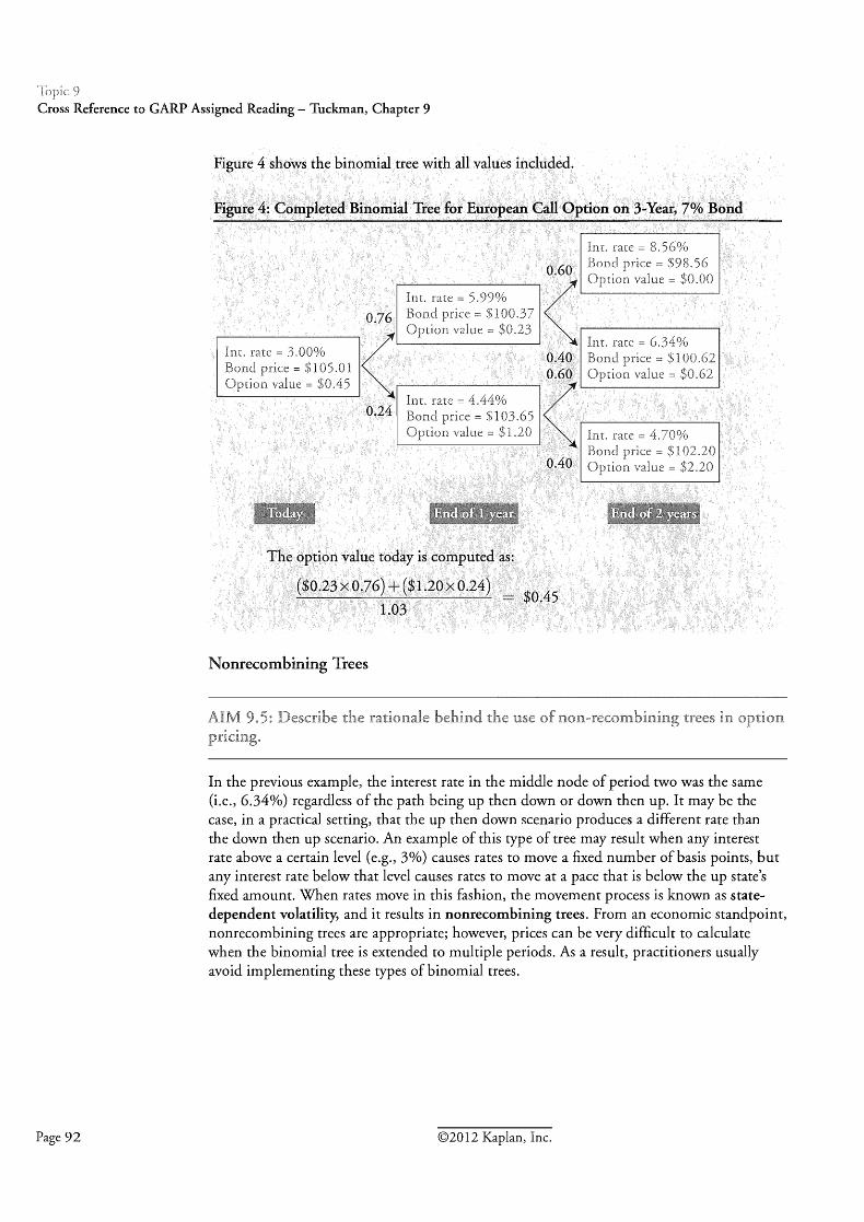
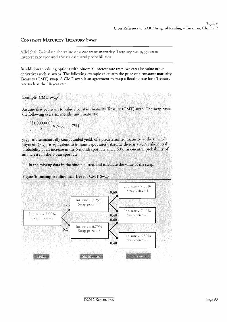
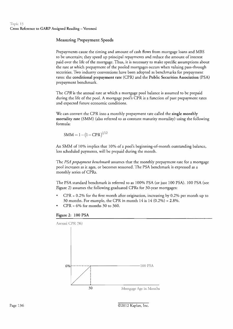
Book 1 Index

sticky delta rule 106 sticky strike rule 105 stipulated trade 153 subordination 15 1 subprime (B-grade) loans 12 1 support tranche 142 surrogate density function 25

tail dependence 36 TBA trade 153 term structure yield volatility 162 total return analysis 166 tracking error VaR 62 Tranche Z 14 1 true probabilities 89 Type I error 50 Type I1 error 50

uncommitted pipeline 153 unconditional coverage 53 undiversified VaR 6 1

value at risk 1 1,43 variance reduction technique 165 variance swap 1 15 volatility skew LO2 volatility smiles 102 volatility surface 105 volatility swap 1 15 volatility term structure 105 volatility-weighted historical simulation 27

weighted average coupon 13 5 weighted average maturity 13 5

yield-based DVO 167

zero-cost product 1 1 1 zero-volatility spread 164

020 12 Kaplan, I&. Page 20 1

020 - our blog · pdf filecandidates enrolled in the online class also have access to...

Documents