04 - u.s. doe office of science (sc)

04

U.S. Department of Energy • Office of Biological and Environmental Research June 2017

Research Priorities to Incorporate Terrestrial-Aquatic Interfaces in Earth System Models Workshop

September 7–9, 2016

Convened by

U.S. Department of Energy

Office of Science

Office of Biological and Environmental Research

Co-Chairs

Organizers

Vanessa Bailey, Ph.D.Pacific Northwest National Laboratory

Joel Rowland, Ph.D.Los Alamos National Laboratory

J. Patrick Megonigal, Ph.D.Smithsonian Environmental Research Center

Tiffany Troxler, Ph.D.Florida International University

Climate and Environmental Sciences Division

Jared DeForest, Ph.D.

Daniel Stover, [email protected]

301.903.0289

This report is available at science.energy.gov/ber/community-resources/ and tes.science.energy.gov.

Mission

The Office of Biological and Environmental Research (BER) advances world-class fundamental research programs and scientific user facilities to support the Department of Energy’s energy, environment, and basic research missions. Addressing diverse and critical global challenges, the BER program seeks to understand how genomic information is translated to functional capabilities, enabling more confident redesign of microbes and plants for sustainable biofuel production, improved carbon storage, or contaminant bioremediation. BER research advances understanding of the roles of Earth’s biogeochemical systems (the atmosphere, land, oceans, sea ice, and subsurface) in determining climate so that it can be predicted decades or centuries into the future, information needed to plan for future energy and resource needs. Solutions to these challenges are driven by a foundation of scientific knowledge and inquiry in atmospheric chemistry and physics, ecology, biology, and biogeochemisty.

Suggested citation for this report: U.S. DOE. 2017. Research Priorities to Incorporate Terrestrial-Aquatic Interfaces in Earth System Models: Workshop Report, DOE/SC-0187, U.S. Department of Energy Office of Science. tes.science.energy.gov.

i

June 2017 U.S. Department of Energy • Office of Biological and Environmental Research

DOE/SC–0187

Research Priorities to Incorporate Terrestrial-Aquatic Interfaces in

Earth System Models

Workshop Report

Electronic Publication: February 2017

Print Publication: June 2017

Office of Biological and Environmental Research

ii


Terrestrial–Aquatic Interfaces

iii


Preface and Acknowledgements

The terrestrial-aquatic interface (TAI) is a highly dynamic component of the Earth sys-tem, developed from a near balance between

terrestrial and aquatic conditions and forming unique processes and community assemblages. Furthermore, TAIs are known to play a critical role in carbon bio-geochemical cycling and have the potential to provide major feedbacks to the Earth system (e.g., methane production). However, there is a lack of basic data and multiscale models to adequately describe how a chang-ing climate can influence the key processes (also an unknown) related to Earth system–relevant feedbacks in these unique, ubiquitous ecosystems.

In general, Earth system models (ESMs) have excluded TAI ecosystem processes, thus creating tremendous uncertainty as to how TAIs will influence climate feed-backs across a range of scales, spanning from local to global. For example, ESMs represent wetlands very sim-plistically at best (e.g., the Accelerated Climate Model-ing for Energy project) and include only a static fraction of dry land or open water, entirely lacking key processes in these hybrid areas and critical climate and biological feedbacks between land and water. This new area of research, therefore, must integrate a variety of import-ant research topics—plants, soil, hydrology, reactive transport, microbiology, genomics, and modeling—into a systems-level understanding that can be extended to improve predictive modeling capabilities.

The goal of the September 2016 Research Priorities to Incorporate Terrestrial-Aquatic Interfaces in Earth System Models Workshop was to engage the scientific community in an open discussion about critical sci-entific gaps. These gaps and research topics demand

immediate field investigations to gather data for repre-senting these important, yet understudied and under-represented, ecosystems in ESMs. Workshop results will inform the U.S. Department of Energy’s Office of Biological and Environmental Research (BER) as it plans and prepares for future research efforts that address the TAI gap through model-informed and model-inspired field studies. The resulting data will enable iterative refinement of high-resolution, next-generation ESMs. Specifically, the workshop (1) summarized past and current field, process, and modeling TAI research; (2) identified critical sensitivi-ties and uncertainties in the systems; (3) identified key processes, traits, existing data, and environmental vari-ables needed to adequately characterize these systems; and (4) discussed idealized strategies that couple mod-els and experiments to advance the state of the science in TAI modeling, including potential experiments that would test and improve land model fidelity.

Given the integrative nature of TAIs, the success of future research efforts necessitates the coordination and collaboration of numerous federal agencies based on their particular expertise and mission. This work-shop defined TAIs by a set of common processes that dramatically influence the Earth system, encompassing both coastal ecosystems (e.g., salt marshes and man-grove forests) and inland wetland ecosystems (e.g., peatlands, floodplains, and wet meadows). Common traits among all these ecosystems are that they are carbon rich; have great potential for carbon dioxide and methane flux; are globally ubiquitous; and are sensitive to climate changes through rising sea level, altered water table, and drought. The workshop did not

iv


consider TAIs that are weighted heavily as aquatic (e.g., open water systems, seagrass meadows, or mud flats).

BER appreciates the tireless efforts of the workshop organizers, co-writers, and contributors who vigorously participated in workshop discussions and generously gave their time and ideas to this important activity. The workshop would not have been possible without the scientific vision and leadership of its organizing com-mittee. BER also extends special thanks to the speakers who gave thought-provoking presentations: Vanessa Bailey, Scott Fendorf, Ruby Leung, William McDowell, Patrick Megonigal, Peter Raymond, Joel Rowland, Tif-fany Troxler, and Kelly Wrighton. In addition, session rapporteurs deserve acknowledgement for capturing the ideas discussed in breakout sessions for use in the

creation of this report: Ben Bond-Lamberty, Elizabeth Canuel, Ethan Coon, Heida Diefenderfer, Scott Fen-dorf, Adam Langley, Melanie Mayes, Rebecca New-comer, Peter Raymond, and Peter Thornton. Lastly, BER lauds the efforts of the workshop writing team who created this document: Vanessa Bailey, Brian Ben-scoter, Ben Bond-Lamberty, Elizabeth Canuel, Ethan Coon, Heida Diefenderfer, Scott Fendorf, Adam Lang-ley, Patrick Megonigal, Peter Raymond, Joel Rowland, James Stegen, Peter Thornton, and Tiffany Troxler.

Also acknowledged are the outstanding efforts of the staff from Oak Ridge National Laboratory’s Biological and Environmental Research Information System, who helped create the workshop visuals and edited and pre-pared this report for publication.


v


Table of Contents

Executive Summary ..................................................................................................................vii

Chapter 1: Workshop Summary, Purpose, and Objectives .................................................... 1

Chapter 2: Introduction to Earth System Science at the Terrestrial-Aquatic Interface ..................................................................................................5

Chapter 3: Processes Across Watersheds to Coasts .............................................................17

Chapter 4: Drivers, Disturbance, and Extreme Events .........................................................35

Chapter 5: Current State of Terrestrial-Aquatic Interface Modeling ..................................41

Chapter 6: Critical Research Needs .........................................................................................49

Chapter 7: Summary and Priorities .........................................................................................57

Appendices: .......................................................................................................................... 61

Appendix 1: Federal Interagency Coordination and Collaboration .............................................. 63

Appendix 2: Agenda ............................................................................................................................ 65

Appendix 3: Workshop Breakout Questions .................................................................................... 67

Appendix 4: Workshop Participants .................................................................................................. 69

Appendix 5: References ...................................................................................................................... 73

Acronyms and Abbreviations .......................................................................Inside back cover

vi



vii


Executive Summary

What are Terrestrial-Aquatic Interfaces?

Terrestrial-aquatic interfaces (TAIs) are dynamic and com-plex components of the Earth system that are transitional between fully terrestrial and fully aquatic environments.

They possess unique biological, hydrological, and biogeochemi-cal attributes that produce exceptionally high rates of biological productivity and biogeochemical cycling. These TAIs regulate the Earth system at a level that far exceeds the area they occupy. They capture, store, transform, and release carbon, nitrogen, phos-phorus, sediments, water, and energy, thereby participating in Earth system cycles that ultimately feed back on the atmosphere, climate, and aquatic ecosystems. Recent developments clearly indicate that a comprehensive understanding of the Earth system is possible only with a detailed understanding of the phenomena that occur where terrestrial and aquatic ecosystems meet (see side-bar, Terrestrial-Aquatic Interface Dynamics, this page).

The past decade witnessed significant advances in understanding the role that Earth biomes play in regulating the Earth system. New Earth system research in terrestrial biomes includes studies in tropical forests, temperate forests, boreal peatlands, and Arctic landscapes. Knowledge of the local, regional, and global carbon budgets of aquatic ecosystems (e.g., rivers, lakes, estuaries, and oceans) has improved significantly, enabling new understanding of the important role these components play in the global carbon cycle. However, research efforts in terrestrial and aquatic systems have been largely independent of one another, championed by separate communities of scientists and agencies. Generally, Earth system research focused on TAIs has been the purview of groups who specialize in ecosystems such as wetlands that typically form at such interfaces. These separate efforts have converged on the conclusion that TAI systems are global “hot spots” of biological, biogeochemical, and ecological activities that are critical to the planet-wide Earth system. The next frontier in developing a holistic

Terrestrial-Aquatic Interface Dynamics— A Large Source of Uncertainty in ModelingThe critically important terrestrial- aquatic interface is not characterized by geographic location or ecosystem type; rather, it is defined by physical interactions that drive keystone pro-cesses. This interface is not merely a conduit for the exchange of soluble and particulate materials between soils and water bodies; it is biogeo-chemically and hydrologically dynamic, transforming the materials that flow through the system.

Because steep process gradients in spatially compressed zones charac-terize these interfaces, there is insuffi-cient understanding of these process dynamics, which often are inferred only by comparing measurements of fluxes into and out of the interfaces. This limited knowledge is a large source of uncertainty in global and regional carbon, environmental, and climate models, significantly impeding the ability to couple models across tra-ditional process and research domains in meaningful and robust ways.

viii


understanding of Earth surface processes is to explicitly couple the dynamics of terrestrial and aquatic systems at their interface. This challenge is daunting because of the many unique processes that arise in TAIs.

Terrestrial-aquatic interfaces often are classified as wetlands, marshes, mangroves, swamps, peatlands, floodplains, riparian zones, hyporheic zones, lake mar-gins, groundwater seeps, and similar transitional areas. However, such designations fail to articulate the unique traits that make TAIs important features of the Earth system. Indeed, the characteristic processes controlling their formation and functioning best define TAIs. These interfaces support unique biological communities, rapid rates of biological productivity, and microbial activity. Although TAIs are limited locally in areal extent, they collectively form a spatially extensive global network that regulates the planet’s biogeochemical cycles.

These systems exhibit high temporal and spatial varia-tion in oxygen supply, have carbon-rich soils, are high potential greenhouse gas emitters, and are sensitive to anthropogenic disturbances (e.g., pollution and fire) and climate change impacts. One useful consequence of defining TAIs by the processes they support is that the boundaries between systems are realistically vague and dependent on the distribution of relevant processes of interest. From a terrestrial perspective, the distribution of processes may be steepest near the physical boundary between domains, diminishing rapidly into the aquatic realm but attenuating grad-ually over large distances into the terrestrial realm. The reverse perspective is likely for research interests that lie predominantly in estuaries, large rivers, and open water. Defining TAIs in this way encourages the development of observational and modeling approaches that span these upland-aquatic transitions, while remaining faithful to the process representations required within purely aquatic and terrestrial systems.

Why are Terrestrial-Aquatic Interface Systems Unique and Important?Perhaps the most important feature of TAI systems from an Earth science perspective is their role as hot

spots and “hot moments” of biogeochemical activity. Examples of processes that peak in TAIs include net primary production, net ecosystem production, denitri-fication, sediment deposition, export of organic and inorganic carbon, and emissions of greenhouse gases.

Terrestrial-aquatic interface systems affect global cycles more prominently than expected based on the proportion of the land surface they occupy because TAIs support exceptionally high rates of Earth sys-tem and environmental processes.

Hydrology is a key feature of TAIs, in part, because water is an effective barrier to oxygen diffusion and creates a sharp boundary separating areas dominated by aerobic versus anaerobic microbial activity. Gradi-ents in oxygen availability are relevant at scales ranging from soil pore spaces to landscapes. The anaerobic microsites of fully terrestrial (upland) soils rapidly transition into an anaerobic matrix across a water- saturated boundary, whether it be the water table sur-face in a soil profile or an upland-to-wetland transition along an elevation gradient. In places where water reg-ularly rises to the soil surface, there are distinctive veg-etation communities dominated by plant species that tolerate anaerobic conditions. In TAIs, organic carbon, oxygen, and nutrients required by plants and microbes for growth and respiration come from the terrestrial or aquatic systems adjacent to groundwater and surface water and from in situ production by plants and micro-organisms in the TAI itself.

Elements, compounds, and matter that originate in terrestrial systems are dramatically transformed in TAIs before they emerge in adjacent aquatic systems. The nature of these transformations is controlled by the hydrologic flow path across TAIs and the traits of plant, animal, and microbial species that dominate these inter-faces. Plants and microorganisms in TAIs add elements, compounds, and particulate matter directly into adja-cent aquatic ecosystems via water discharge. Thus, TAIs


ix


exert an overwhelming influence on the biogeochemis-try and ecology of aquatic ecosystems.

Dynamic change, or the potential for change, is a com-mon feature to most TAIs. Consequently, TAIs differ from other ecosystem types in that relatively subtle changes in their boundary conditions can affect the very existence and spatial location of TAIs. There is a high potential for state change or ecosystem collapse with minor changes to vegetation or surface properties. For instance, many tidal wetlands build soil vertically by trapping exogenous and in situ sediment, thus gain-ing elevation with sea level rise, and the perturbations to sediment supply can convert the wetlands to mud flats or open water. Dramatic state changes often are irreversible on a human time scale and have enormous consequences for biogeochemical cycles. TAIs are particularly vulnerable to the pressures of climate and environmental changes such as those in precipitation patterns, sea level rise, increasing salinity, and the frequency of extreme events. These events that are known to influence TAIs include short-term, pulse-type disturbances such as fire and storm surges and the more persistent, press-type events such as drought, altered plant species composition, and groundwater extraction. Therefore, a robust understanding of TAIs requires a focus on their dynamic properties that are most sensitive to change, specifically the hydrologic continuum between terrestrial and aquatic ecosystems, accompanying reduction-oxidation and transport proc esses, and plant-microbe community ecology.

Scale is an inherent property of natural systems that poses special challenges in TAIs. Conceptually, TAIs and their distinctive processes exist across vast spatial (and temporal) scales, ranging from micrometer-scale oxygen gradients in soil aggregates to kilometer-scale transitions in ecosystems across elevation gradients. Overlain on the spatial scale is shape; TAIs at all scales typically are irregularly shaped features that are diffi-cult to observe, quantify, and model. Scaling processes within a specific type of ecosystem is a challenge, but far more challenging is coupling terrestrial and aquatic systems because each operates at distinctly different

temporal and spatial scales. The multiscale nature of temporal and spatial gradients across interfaces rep-resents one of the greatest challenges in Earth system research—one that requires the integration of physics, hydrology, biogeochemistry, biology, and Earth system feedbacks.

What is the State of Knowledge at the Terrestrial-Aquatic Interface?The U.S. Department of Energy’s Office of Biological and Environmental Research (BER) held the Research Priorities to Incorporate Terrestrial-Aquatic Interfaces in Earth System Models Workshop in Washington, D.C., on September 7–9, 2016. BER sponsored the workshop for scientists who study terrestrial, aquatic, and TAI systems to assess the state of the science in coupled terrestrial and aquatic ecosystems and to develop a strategy for advancing Earth system research at the TAI. The assembled group agreed that there is a lack of observational data and models required to ade-quately understand the key ecological, biogeochemi-cal, hydrological, and physical processes that interact in TAIs and feed back on the Earth system. Also rec-ognized were that terrestrial, TAI, and aquatic systems each operate with fundamentally different temporal and spatial dynamics and that coupling across such sys-tems will require conceptual advances, new observa-tions, coordinated experimental efforts, new modeling frameworks, and transdisciplinary research teams.

Existing observations and models of surface and sub-surface hydrology, biogeochemistry, plant ecology, and microbial ecology fail to address key knowledge gaps unique to TAIs. Gaps often are related to the fact that processes operate at fundamentally different tempo-ral and spatial scales in terrestrial systems compared to those in the aquatic ecosystems to which they are coupled. There is limited understanding to inform decisions about scaling up a system response such as methane (CH4) emissions—when to use an empirical approach versus process-based numerical models. Identifying the need for upscaling and developing the appropriate methodologies to achieve it are essential

Executive Summary

x


for incorporating knowledge gained from multiscale experiments into predictive multiscale models. An inability to predict such scale transitions may indicate structural deficiencies in the models themselves. In that case, new experiment-model iterations would be needed to elucidate processes that cause observed scale dependencies.

Advances in TAI science will require a creative com-bination of experimental manipulations, cross-system observations, and multiscale numerical and statistical models. Research in this field can advance quickly by integrating models and empirical science into a com-prehensive program designed to (1) provide empirical constraints (likely varying across systems) to calibrate and evaluate models and (2) reveal mechanisms need-ing improvements in process-based predictive models.

Key Gaps and Research Recommendations for Terrestrial-Aquatic Interface ScienceBecause TAIs are globally ubiquitous, achieving a fundamental understanding of the hallmark processes in these systems requires extending system-specific observations to a globally relevant knowledgebase and, for the first time, coupled terrestrial, aquatic, and TAI models. Ignoring these critical interfaces clearly limits the ability to couple the largest features of the Earth system—land, water, and ocean—to achieve a fully comprehensive understanding of the global system. Workshop participants identified several research chal-lenges to focus these efforts:

■ The size and shape of TAIs have prevented an accurate accounting of their locations, areal extent, species composition, and basic ecosystem inven-tories such as carbon and nutrient pools. An exact accounting of stocks, fluxes, and transformations in TAIs is a fundamental need that requires accurate, high-resolution maps and digital elevation models. Such information continues to elude TAI scientists but is needed before spatial models can represent TAI processes.

■ Hydrology is a fundamental control on biological, biogeochemical, and geomorphological processes in ecosystems. Hydrologic observations and models tend to focus on specific types of systems such as terrestrial ecosystems, rivers, estuaries, or ground-water. Advancing TAI science requires cross-system hydrologic observations and models that explic-itly account for interactions between surface and groundwater as the water moves through TAI plant communities and soils.

■ Plants exert a second level of fundamental control on biological, biogeochemical, and geomorpholog-ical processes in TAIs. Plant species in TAIs share highly specialized traits for tolerating anaerobic conditions, flooding, salinity, sediment deposition, and other sources of stress. Although the physio-logical and morphological bases of such traits are well understood, their response to factors such as elevated carbon dioxide (CO2) or changes in hydrology or environment is generally not well known. Thus, these traits and responses are poorly represented in models of any kind including envi-ronmental and Earth system models. This limited understanding of the responses of specialized plant traits to global change is a gap in TAI science.

■ Microorganisms interact with plants and plant- derived or plant-transported substrates to cycle carbon, nutrients, and pollutants in TAIs. The juxtaposition of aerobic and anaerobic conditions that exist at the interface supports rapid rates of microbial activity and uniquely coupled processes. Because plants are sources of organic carbon (e.g., energy) and respiratory substrates (e.g., oxy-gen) and are conduits for emitting greenhouse gases (e.g., CO2 and CH4), these systems cannot be understood without mechanistic knowledge of microbe-plant interactions. Microbial processes in the plant rhizosphere represent significant uncer-tainty and a knowledge gap in the understanding of TAIs. Understanding these processes is essential for inclusion in models.


xi


■ TAI systems are highly dynamic features that move, expand, or contract at time scales of hours to years. Changes can occur in both the vertical and horizon-tal dimensions and be driven by changing hydrology, sediment supply, plant community composition, or chemical inputs in high-frequency or short- frequency events. Current observations, experiments, and models do not account for interactions among plant processes, soil processes, and hydrologic proc-esses that drive geomorphic changes across terrestrial to aquatic ecosystem interfaces and boundaries.

■ TAIs are an extreme example of the more general scientific and computational problems surrounding scale. Processes operating at small scales of time and space in TAIs drive large-scale phenomena that cannot be predicted with existing observational or modeling techniques. Scale also presents a challenge when coupling models that were designed to operate as isolated units because terrestrial, TAI, and aquatic systems operate at distinctly different temporal and spatial scales. Advancing TAI science requires cre-ative approaches to combining experiments, models, and observations in ways that respect (rather than ignore) these inherent differences in scale.

■ Highly responsive to perturbations, TAIs are prone to sudden changes in function or wholesale changes in state (e.g., from wetland to aquatic). Internal TAI

processes operating at small scales respond to large-scale external events such as sea level rise, drought, and flooding. Scale-relevant research is needed to predict the impacts of these perturbations on the interface’s relatively narrow zone. A particular chal-lenge will be to forecast how TAI ecosystems (and the terrestrial or aquatic systems to which they are coupled) respond to forcing from external drivers such as changes in climate, environment, and land use. Forecasting changes in function and state requires a more detailed understanding than now exists of the feedbacks inherent in TAI systems that render them resilient to perturbations.

Clearly, human systems need consideration in any study of TAI ecosystems because of the immensity of their effects on key physical and biological processes. Meeting this goal will require the participation of mul-tiple TAI stakeholders including the National Oceanic and Atmospheric Administration, U.S. Geological Survey, U.S. Department of Agriculture, Smithsonian Institution, National Science Foundation, and National Aeronautics and Space Administration. The need for a TAI-focused research program arises from the fact that critical Earth and environmental system processes cross the traditional terrestrial-TAI-aquatic boundaries adopted by funding agencies. As a result, integrated and coordinated research is needed at the terrestrial-aquatic interface to be fully successful.

Executive Summary

xii



CHAPTER 1Workshop Summary, Purpose, and Objectives


Terrestrial-aquatic interfaces (TAIs) are highly dynamic components of Earth and environ-mental systems that lie in the complex transi-

tion zone between terrestrial and aquatic conditions. TAIs are ecosystems with unique plant traits, microbial communities, hydrology, geomorphology, and bio-geochemical processes, but these interfaces also are coupled intimately to biological, physical, and chem-ical processes occurring in adjacent terrestrial and aquatic ecosystems. TAIs play a critical role in carbon, nutrient, and contaminant biogeochemical cycling, and they feed back on Earth and environmental sys-tems through the storage, transformation, and release of elements (i.e., carbon and nitrogen) involved in the production, export, and emission of greenhouse gases such as carbon dioxide, methane, and nitrous oxide. TAI systems also can have a dominant influence on the biology and chemistry of downstream aquatic ecosys-tems and their interactions with the atmosphere.

Advances over the past 2 decades have clearly shown that TAI systems are important in local, regional, and global biogeochemical cycles and that TAI processes must be considered to understand and model the coupling between terrestrial and aquatic ecosystems. Supported by various funding agencies, research programs have made progress by focusing on independent studies of terrestrial, TAI, or aquatic systems. The emerging general consensus is that further progress at improving understanding of the Earth system will require new efforts that explicitly cross these traditional disciplinary boundaries (see Appendix 1: Federal Interagency Coordination and Collaboration, p. 63). However, there is a lack of basic

data and multiscale models to adequately describe and represent how these unique and ubiquitous eco-systems influence Earth system processes. Thus, most Earth system models (ESMs) exclude TAI processes. For example, ESMs incorporate wetlands with very simplistic hydrological, biogeochemical, and plant representations but lack the dynamic feedbacks that capture changes in spatial distribution over seasons or years. This new area of research, therefore, must inte-grate a variety of important research areas—plant and microbial ecology, soil science, hydrology, reactive transport, microbiology, genomics, and modeling—into a robust systems-level understanding that improves predictive modeling capabilities.

The U.S. Department of Energy’s (DOE) Office of Biological and Environmental Research (BER) held the Research Priorities to Incorporate Terrestrial- Aquatic Interfaces in Earth System Models Work-shop in Washington, D.C., on September 7–9, 2016 (see Appendix 2: Agenda, p. 65). BER sponsored the workshop for scientists who study terrestrial, aquatic, and TAI systems to assess the state of the science in coupled terrestrial and aquatic ecosystems and to develop a strategy for advancing Earth system research at the TAI (see Appendix 3: Workshop Breakout Questions, p. 67; Appendix 4: Workshop Participants, p. 69). The workshop’s goal was to identify critical scientific knowledge gaps that limit the ability to rep-resent TAIs in predictive models, supporting the DOE BER mission to understand complex biological and environmental systems. This interface is of particular concern to BER’s Climate and Environmental Sci-ences Division, which leads DOE efforts to enhance

Workshop Summary, Purpose, and Objectives


1

3

Chapter 1 – Workshop Summary, Purpose, and Objectives


predictive capabilities of the Earth system as a whole. The assembled community discussed (1) the state of knowledge with respect to understanding key TAI processes; (2) interdependencies among terrestrial, TAI, and aquatic systems; (3) research tools such as databases, technologies, observational approaches, and models; and (4) key research priorities necessary to improve predictive understanding of this critical eco-system interface.

The workshop affirmed the view that TAI systems are critical interfaces defined by physical, chemical, and biological interactions that produce rapid rates (“hot spots”) of biogeochemical processes. These interfaces are not merely conduits for the exchange of soluble and particulate materials among plants, soils, water bodies, and the atmosphere, but rather biogeo-chemically and hydrologically dynamic bodies where

materials are transformed as they flow through and interact with TAI systems. While TAIs often are clas-sified as wetlands, marshes, mangroves, swamps, peat-lands, floodplains, riparian zones, hyporheic zones, lake margins, groundwater seeps, or similar transitional areas, the workshop highlighted the fact that such designations fail to articulate the unique traits that make TAIs important features of the Earth system. Terrestrial-aquatic interfaces support unique biological communities, rapid rates of biological productivity and microbial activity, high temporal and spatial variation in oxygen supply, carbon-rich soils, high potential greenhouse gas emissions, and sensitivity to anthro-pogenic disturbances and climate change impacts. Although TAIs are limited in global areal extent, at the landscape scale they collectively form a spatially exten-sive network that regulates global biogeochemical cycles (see Fig. 1, this page).

Fig. 1. Areas Dominated by Terrestrial-Aquatic Interfaces (TAIs). TAI ecosystems (dark blue) are ubiquitous across the globe. [Image courtesy U.S. Department of Agriculture Natural Resources Conservation Service]

Chapter 1 – Workshop Summary, Purpose, and Objectives

4



CHAPTER 2Introduction to Earth System Science at the Terrestrial-Aquatic Interface

6


Terrestrial-Aquatic Interfaces as a Concept

Conceptually, the “interface” of terrestrial and aquatic systems calls to mind a sharp bound-ary such as a river bank, a lake shore, the

edge of a salt marsh, or even the top of the water table. However, a helpful approach is to view terrestrial- aquatic interfaces (TAIs) from the perspective of the processes that control the fluxes and transformation of mass and energy in ecosystems that bound such physical interfaces. From this perspective, TAIs take on complex, spatially and temporally dynamic scales. These scales are best defined by gradients in specific processes that are relevant to understanding and quan-tifying fluxes and transformations in Earth and envi-ronmental systems.

The multiscale nature of temporal and spatial proc-ess gradients across TAIs represents one of the great research challenges in Earth science and is a major reason that TAI systems remain poorly understood. For example, in regions with very high rates of phys-ical change and biogeochemical transformation, the relevant scales for both observations and prediction may be on the order of nanometers and seconds. Conversely, system-scale hydrological drivers such as precipitation and sea level rise dictate measurements and predictions at watershed to global scales over years to decades. Coupling such divergent process represen-tations is a fundamental challenge in advancing under-standing and modeling of Earth systems.

The scientific and stakeholder objectives of the observer determine how TAIs are viewed and defined. For a

scientist or stakeholder focused on the coupling of wet-land systems to terrestrial systems, the wetland-aquatic boundary may demarcate areas of primary interest (land-wetland coupling) from areas of less interest (wetland-aquatic coupling). From this perspective, the TAI would extend from the wetland into the terrestrial system over large distances but diminish rapidly from the wetland into the aquatic realm. Conversely, for a researcher focused on estuaries, large rivers, and open water, the TAI may extend from the wetland into the aquatic system over large distances and less so into the terrestrial realm. Development is needed of observational and modeling approaches that span all viewpoints while remaining faithful to the proc ess representations, both within the interface regions and in the more traditional aquatic and terrestrial systems. This scientific challenge requires integrated research across physical, chemical, and biological scientific disciplines and novel modeling strategies both in spatial and process representations and in computational architectures. Interactions inherent in TAIs arise from fundamental Earth and environmental system processes. Hydrology is the most important determinant of TAI structure, function, and variability in time and space. Indeed, TAIs are an inevitable outcome of water cycling within terrestrial and aquatic systems. Water chemistry undergoes dramatic change as precip-itation passes through plant canopies, soils, aquifers, streams, rivers, lakes, and estuaries. In the process, the flow and accumulation of water drive changes in geomor-phology, soils, biogeochemistry, and ecology across ter-restrial, wetland, and aquatic ecosystems. Such changes are especially important where terrestrial and aquatic ecosystems meet across a TAI, including during extreme events such as flooding or low flows.

Introduction to Earth System Science at the Terrestrial-Aquatic Interface


2

7

Chapter 2 – Introduction to Earth System Science at the Terrestrial-Aquatic Interface


Fundamental Concepts Relevant to Terrestrial-Aquatic InterfacesTerrestrial-aquatic interfaces are not passive boundaries across which water, carbon, other solutes, and particles move but dynamic transition zones where hydrology, biology, and geochemistry converge to create high proc-ess rates of outsized importance to element cycling (see Fig. 2, this page). TAIs typically are small in areal extent compared with that of the landscape matrix in which they are embedded, but they are highly important

to biological and geochemical element cycling. Such regions have been referred to as hot spots. The same concept applies to time, associating the term “hot moments” to punctuated periods of intense transport and processing (McClain et al. 2003). These concepts are central to understanding the potential rewards and the challenges of a research initiative focused on TAIs.

Hot spots occur at scales ranging from soil aggregate microsites to large wetlands embedded in landscapes (see Fig. 3, this page). Examples of the range of spatial

Fig. 2. Hot Spot Formation. Terrestrial- aquatic interfaces support high rates of biogeochemical processes because hydrologic flow (arrows) causes two or more reactants to intersect. Two com-mon scenarios are shown. [Modified and reprinted with permission from Springer from McClain, M. E., et al. 2003. “Biogeo-chemical Hot Spots and Hot Moments at the Interface of Terrestrial and Aquatic Ecosystems,” Ecosystems 6(4), 301–12. © 2003 Springer-Verlag New York, Inc.]


Fig. 3. Hot Spots at Multiple Spatial Scales. Terrestrial- aquatic interfaces (TAIs) are classic examples of hot spots, a concept based on differences in process rates in space and independent of scale. TAIs occur at the scale of (a) soil micro-sites, (b, c) hill slopes, (d) small watersheds, and (e) large watersheds. [Modified and reprinted with permission from Springer from McClain, M. E., et al. 2003. “Biogeochemical Hot Spots and Hot Moments at the Interface of Terrestrial and Aquatic Ecosystems,” Ecosystems 6(4), 301–12. © 2003 Springer- Verlag New York, Inc.]

8



scales embodied by the hot spot concept include (1) anoxic microsites within soil aggregates or pedons (Sexstone et al. 1985; Keiluweit et al. 2016); (2) oxic microsites around wetland plant roots (Armstrong and Armstrong 2001); (3) hyporheic flow paths (Hedin et al. 1998; Harms and Grimm 2008); (4) discrete vegetation patches (Troxler et al. 2014); and (5) inter-tidal or semiflooded wetland landscapes (Bridgham et al. 2006). The hot spot concept as applied to TAIs often refers to biological processing of elements under conditions of varying oxygen availability or, more accurately, varying reduction-oxidation (redox) potential. Fluctuations between aerobic and anaerobic conditions drive transformation and cycling of redox- sensitive elements such as carbon, nitrogen, organic matter, iron, manganese, and sulfur. Redox processes in TAI systems ultimately regulate climate and environ-mentally relevant phenomena such as greenhouse gas emissions and preservation of organic carbon in soils. The hot spot–hot moment concept explains a large body of research that shows TAI processes are quanti-tatively important at basin, landscape, and global scales (see sidebar, Hot Spots and Hot Moments, this page). Riparian forests remove as much as 50% of nitrogen loading to streams where hydrologic flow intersects the root zone (Vidon et al. 2010). Coastal wetlands account for 0.2% of ocean area but 47% of organic carbon burial (Nelleman et al. 2009). Small water bodies disseminated across the landscape account for 50% of sediment accumulation and organic matter processing in terrestrial landscapes (Smith et al. 2002). Natural wetlands represent less than 10% of the land surface while constituting the largest single source of atmospheric methane (CH4) and ~30% of mean global emissions (Paudel et al. 2016). Patterns of atmospheric circulation near coasts concentrate dry nitrogen depo-sition over land, creating large-scale hot spots of nitrate (NO3) and ammonium particulate deposition that are two to five times higher over land than water (Lough-ner et al. 2016). The fields of Earth system science and ecohydrology have only recently begun to document the importance of hot spots and hot moments across scales from soil aggregates to hillslopes to watersheds.

Hot Spots and Hot MomentsTerrestrial-aquatic interfaces (TAIs) exhibit very high spatial and temporal variation in biogeochem-ical processes. Process rates in TAIs may differ by orders of magnitude from those in adjacent areas, making these interfaces areas of “outsized” weight in biogeochemical budgets. Ecologists have adopted the terms hot spots and hot moments to describe the phenomena in which small areas or short time periods account disproportionately for changes in a process of interest. TAIs are classic examples of hot spots and hot moments. The same concept exists in other disciplines; hydrology recognizes hot spots in the form of preferential flow paths and hot moments in the form of peak flows. The terms connote the rel-ative magnitude of a process, not necessarily the fre-quency. A hot spot can be continuous over time and hot moments can occur regularly. The terms are not typically used as synonyms of extreme events, which tend to be less predictable.

Moreover, only recently have predictive models incor-porated hot spots that describe nutrient dynamics in TAI systems (Arora et al. 2015).

Terrestrial-aquatic interface systems must be under-stood as more than boundaries or transition zones, rather as unique ecosystems in and of themselves. Characterized by a tight interdependence of hydrology, soils, plants, and microbes, TAIs produce unique bio-logical communities compared to their terrestrial and aquatic counterparts.

The location of TAIs at boundaries between land, ocean, and rivers makes them highly susceptible to extreme hydrological and weather events such as hurri-canes and floods. Although such events constitute hot spots and hot moments in the strictest sense, they tend to be far less predictable and are better described as “extreme events.” These events cause sudden, dramatic, and transitory changes in environmental conditions

9



that have long-term consequences for ecosystems. For example, Hurricane Andrew caused intense mortality of mangrove forests in the southwest coastal region of Florida (Doyle et al. 1995). By contrast, sediment deposition from Hurricane Wilma increased mangrove soil fertility and soil elevation, both of which may have long-term benefits for mangrove forest produc-tivity (Castañeda-Moya et al. 2010). Thus, extreme events can cause positive or negative feedbacks on TAI ecosystem structure and function, depending on the event’s intensity and frequency (Conner et al. 2014). The impact of extreme events is more likely to be negative (e.g., sea level rise) in systems already com-promised by human activities such as water diversions, but the feedbacks between such events and ecosystem structure and function are poorly understood.

Human activity is an important source of disturbance in TAI systems (Pelletier et al. 2015). These interfaces are highly sensitive to changes in climate, environment, and land use, because TAIs are strongly influenced by local and nonlocal drivers. Coastal regions and river corridors are often areas with the greatest population densities and land-use intensities. Both of these factors increase the likelihood of sudden changes in ecosystem structure and function resulting from disturbance and limit a system’s capacity to adjust to change. Coastal wetlands show a high capacity to adapt to sea level rise (Kirwan and Megonigal 2013) and high susceptibil-ity to “marsh drowning” (Voss et al. 2013). In time, extreme events may become more common in many regions (Katz and Brown 1992; Milly et al. 2008), and human activities may continue to alter TAIs. Thus, the scientific community must seek to understand and develop new tools to analyze a future for which there are no historical analogues that include exposure of TAIs to chronic instability and fluxes.

Historical Perspectives on Terrestrial-Aquatic InterfacesScientists working in a wide variety of disciplines have developed a rich reservoir of concepts, data, and models that relate in some fashion to TAI systems

but have never integrated these elements to advance a holistic understanding of Earth system science. Several proposed conceptual frameworks explain changes in the relative importance of TAI processes across spatial scales from headwater basins to coastal zones. These concepts include a river continuum (Vannote et al. 1980), nutrient spiraling (Newbold et al. 1981), hyporheic corridors (Stanford and Ward 1993; Harvey and Gooseff 2015), flood pulse ( Junk et al. 1989), outwelling (Odum 1980), and the wetland donor-receptor-conveyor (Brinson 1993). Scientists can use elements of such conceptual frameworks to develop a holistic understanding and modeling frame-work for TAI processes. For example, under the river continuum concept (see Fig. 4, p. 10), governing the flux of materials that move from terrestrial systems to surface waters are streambed physical dimensions and the characteristics of near-shore vegetation, such as stem density that affects hydrology. In this case, narrow (generally low-order) streams maximize fluxes of terres-trial material into surface water, while wide (generally higher-order) streams and rivers maximize the poten-tial for uptake of terrestrial material, such as terrestri-ally derived inorganic nutrients, by in-stream primary producers. All these conceptual frameworks highlight important interactions and connections whereby (1) geomorphic features provide the physical template across and through which water moves; (2) water flow and spatial distribution strongly influence the availabil-ity of resources to biological agents; and (3) biological agents transform resources in ways that influence their fate [e.g., mineralization of dissolved organic matter to carbon dioxide (CO2)]. Despite this rich conceptual framework, only recently has the scientific community fully appreciated the quantitative importance of TAI processes to the Earth system.

With the community’s evolving view of the role of these systems in regional and global budgets, many groups are integrating representations of TAI proc-esses into Earth system models (ESMs) to a limited extent (e.g., wetland processes; for a review, see Xu et al. 2016a). The history of efforts to model the

10



DOE/SC-0187

Fig. 4. Terrestrial-Aquatic Interfaces (TAI) Continuum. This illustration shows the differences in spatial scale of some of the commonly studied systems that TAI research seeks to integrate, namely interfaces associated with headwater streams, rivers, wetlands and floodplains, estuaries, and coasts. These subsystems are con-nected to one another through hydrology, geomorphology, solute and particulate transport, and ecological relationships, forming an integrated terrestrial-aquatic continuum from land to ocean.

11



global carbon cycle illustrates how TAI concepts have changed. Early box models of the Earth’s carbon cycle included lateral carbon transfer from land to the ocean (Sarmiento and Gruber 2002; Schlesinger and Bernhardt 2013). However, there was no processing of terrestrial carbon either at TAIs or in the water bod-ies through which carbon moved before reaching the ocean. Now clearly evident is that the transformation of terrestrial materials in TAI systems is quantita-tively important in Earth and environmental systems. Although modest advances have been made in model-ing these processes, they are isolated within TAI or riv-erine systems. Indeed, there have been minimal efforts to couple terrestrial-TAI-aquatic processes. As the fol-lowing discussion indicates, where progress has been made, the TAI system still is often treated as a bound-ary condition of the terrestrial or aquatic system rather than as a separate system. The goal of such models was to understand carbon and nutrient flux and processing in fully aquatic systems, with no attention paid to trans-formations occurring in TAIs.

The original conceptualization of aquatic systems was that of a passive pipe because transformations were not known to occur during transport through the aquatic continuum (Cole et al. 2007; see Fig. 5a, this page). Continuing with the carbon cycle example, this concept began to change with reports of substantial CO2 degassing from aquatic systems (Richey et al. 2002; Frankignoulle et al. 1998) and significant carbon burial during transport (Tranvik et al. 2009; Sabine et al. 2004). These studies led to a reconceptualization of aquatic systems as active pipes where transforma-tions of terrestrial carbon occur (Cole et al. 2007; see Fig. 5b, this page). A recent elaboration in the form of the Pulse-Shunt Concept recognizes that large “pulse” releases from terrestrial systems “shunt” materials downstream, bypassing areas where processing nor-mally would occur and effectively changing the active pipe into a passive pipe (Raymond et al. 2016). TAI systems such as wetlands are captured by these active-pipe concepts but also are considered to be either ter-restrial or fully aquatic systems. The TAI concept takes

these conceptual models a step further by acknowledg-ing that TAI systems lie between those that are fully aquatic or terrestrial, have unique carbon cycles, and exercise important control over net fluxes of CO2 and

Fig. 5. Conceptual Models of the Coupling Between Terrestrial and Ocean Carbon Cycles. (a) Aquatic systems transport terrestrial carbon to oceans with little or no processing. (b) Aquatic systems actively remove terrestrial carbon during transport through deposition of particulate car-bon in sediments and microbial mineralization of organic carbon to carbon dioxide. Terrestrial-aquatic interfaces (TAIs) such as wetlands generally are considered to be part of the terrestrial system. (c) Represented as distinct systems, TAIs share both terrestrial and aquatic characteristics. TAIs can act as both net sinks (black arrows) and sources (green arrows) of carbon to aquatic systems and the atmo-sphere under different conditions. [Modified and reprinted with permission from Springer from Cole, J. J., et al. 2007. “Plumbing the Global Carbon Cycle: Integrating Inland Waters into the Terrestrial Carbon Budget,” Ecosystems 10, 172–85. © 2007 Springer Science+Business Media, LLC]

a.

b.

c.

12



particulate carbon (see Fig. 5c, p. 11). For example, wetlands are TAI systems where terrestrially derived carbon is deposited, buried, and preserved and where CO2 evasion takes place; thus, wetland processes dra-matically control the size and nature of carbon fluxes. Plant production within TAIs is the largest source of organic matter preserved in TAI soils. Changes in plant growth resulting from elevated CO2, flooding, or other factors not only alter carbon inputs, but can change a “stable” carbon pool into an “unstable” pool by increas-ing the availability of organic carbon and oxygen (Mueller et al. 2016; Wolf et al. 2007). Likewise, TAI systems such as tidal marshes are sources of dissolved organic carbon for aquatic systems and regulate proc-esses such as photochemical and microbial carbon processing during transport from a TAI to receiving waters (Vähätalo and Wetzel 2004; Tzortziou et al. 2007, 2011).

Despite the progress made in including aquatic ecosystems in carbon budgets, the role and con-tributions of TAIs and fully aquatic ecosystems in storing and transporting carbon are not clear, and this knowledge is necessary for a proper determina-tion of their importance. A recent analysis of carbon exported from terrestrial soils to aquatic systems suggests that storage along the continuum of fresh-water bodies, estuaries, and coastal rivers may be much greater, by 0.5 petagrams of carbon per year, than previously thought (Regnier et al. 2013). This finding has important implications for understanding of the global carbon budget. For example, budgets of carbon flux through terrestrial-TAI-aquatic systems have been used to (1) constrain hydrologic controls on atmospheric CO2 levels through time (Berner 1994; Maher and Chamberlain 2014), (2) estimate the net flux of CO2 between the ocean and atmo-sphere ( Jacobson et al. 2007), and (3) balance the production and oxidation of organic matter on land (Sarmiento and Gruber 2002).

Understanding of nutrient fluxes also has evolved considerably. Many studies in recent decades have elu-cidated key controls on terrestrial nutrient transfers to

the aquatic continuum. In general, research has docu-mented a strong anthropogenic influence on nutrient fluxes from agriculture and urban land management ( Jordan and Weller 1996; Coutler et al. 2004; Brous-sard and Turner 2009). TAI and aquatic processes are clearly important in the uptake, transformation, and burial of nutrients in landscapes, and large amounts of anthropogenic nutrients may be stored and mobilized in future years despite the successful management of nutrient loading (Powers et al. 2016). Furthermore, models indicate that rapid climate and other environ-mental changes could mobilize a greater percentage of important nutrients to TAIs, streams, and rivers due to a decrease in residence time in the terrestrial systems from where they originate (Howarth et al. 2012).

Models of Coupled Terrestrial, TAI, and Aquatic ProcessesHistorically, the needs specific to terrestrial, certain wetland ecotypes, or aquatic ecosystems have driven models of TAI processes and systems. Further, very few of these models attempted to couple the full suite of processes that occur across terrestrial-TAI-aquatic systems (see Fig. 6, p. 13). In ESMs, processes taking place in TAIs such as nontidal mineral soil wetlands, coastal wetlands, and peatlands are simulated using modules designed for upland ecosystems. ESMs do not have mechanistic modules to describe the bio-geochemical transformations that occur as materials flow across TAIs from upland to aquatic systems. Although the ability to model biogeochemical trans-fers at regional to global scales has evolved (e.g., for the leaching of NO3 fluxes; Zhu and Riley 2015), there is a need for significant improvement. Many models use nutrient fluxes measured or estimated at the scale of large basins to continents, capturing the aggregated effects of transport and processing but missing critical hot spots at the TAI scale. Further-more, most key processes in these models are repre-sented at long temporal scales despite a growing body of literature stressing the importance of short-term, transient hydrologic events in controlling nutrient

13



Fig. 6. Carbon Movement Through Terrestrial-Aquatic Interfaces (TAIs). Water is a key agent, moving biogeochemical constituents through the atmosphere and the TAI continuum. (1) Atmo-spheric particles promote cloud formation. (2) Raindrops absorb carbon, carrying it to Earth. (3) Other carbon sources in the atmosphere include burning and gas fluxes [e.g., carbon diox-ide (CO2)]. (4) Plants fix CO2 through photosynthesis, converting it into more complex forms of biomass. (5) Plant litters and exudates enrich the soil with organic carbon. (6) Water transports carbon through forest canopies (throughfall and stemflow), and biogeochemical transformations occur in soils and sediments and during overland flow. (7) Organic carbon is decomposed micro-bially and abiotically, returning CO2 to the atmosphere and producing biomass and metabolites. (8) Carbon is stored and transformed in open water bodies. (9) River plumes may be enriched in nutrients. (10) Coastal marshes can both store and export carbon. (11) Continental shelves and oceans can absorb atmospheric CO2, biologically storing carbon in (12) marine sediments. [Reprinted under a Creative Commons Attribution License (CC BY) from Ward, N. D., et al. 2017. “Where Carbon Goes When Water Flows: Carbon Cycling Across the Aquatic Continuum,” Frontiers in Marine Science 4, 7. © 2017 Ward, Bianchi, Medeiros, Seidel, Richey, Keil, and Sawakuchi]

14



export trajectories and magnitudes (Hall et al. 2013; Raymond et al. 2016).

The vegetation models for TAI systems are in their infancy. For instance, the transport of gases (e.g., oxygen and CH4) through wetland plants is a critical feature of some TAIs that is needed to model carbon and green-house gas dynamics. The wetland biogeochemistry modules in both the Community Earth System Model and the Accelerated Climate Modeling for Energy project represent these processes by using upland plant production and respiration to drive the production of CH4 and transport it and other gases through hypothet-ical wetland plant tissues (Riley et al. 2011). Similarly, vegetation models in ESMs do not have explicit repre-sentations of how salinity affects vegetation growth and mortality in coastal zones and, therefore, cannot mech-anistically explore carbon-nutrient feedback in tidal wetland ecosystems. Finally, most models have only static vegetation distributions, which lack the ability to dynamically respond to changes in important drivers such as flooding frequency and salinity or use simple formulations that ignore key physiological processes such as photosynthetic rates, flooding stress, salinity stress, and intraspecific competition (Ge et al. 2016). Such models almost certainly will fail to correctly simulate realistic vegetation responses and associated interdependencies or feedbacks under future novel cli-mate conditions.

Terrestrial-Aquatic Interfaces as a Transdisciplinary ChallengeThe involvement of numerous scientific disciplines, each of which contributes to the study of wetlands, rivers, and coasts, is evident from the background described in this section. In general, they include the classic marriage of the environmental and life sciences that established the foundation of ecology (Moore 1920). Some of the more important environmental science fields that address TAI systems include hydrol-ogy, meteorology, oceanography, geology, and geo-morphology. Among the important life sciences are ecology, microbiology, and plant physiology. Hybrid

disciplines that encompass biotic and abiotic com-ponents also are highly relevant, such as limnology, biogeoscience, ecohydrology, ecogeomorphology, soil science, and ecology.

The increasingly large number of disciplines required by research teams to address complex problems is now the rule, not the exception (Börner et al. 2010; Ledford 2015). Arguably, the inherent need to bring multiple disciplines to address research problems in terrestrial-aquatic ecosystem science is the very reason that such large research gaps remain—historically, interdisciplinary studies have received low levels of funding (Bromham et al. 2016). There are rich scien-tific literatures to be mined in the ecology of wetlands, riparian zones, forests, coastal systems, estuaries, landscapes, soils, and other nonecological-centric disciplines such as hydrology and climate change sci-ence. The breadth and diversity of these disciplines pose distinct challenges for TAI research if disciplinary activities remain independent and fragmented. For instance, different disciplines use different vocab-ulary words to describe the same phenomena and different theoretical frameworks to underpin research and modeling approaches; furthermore, researchers attend disciplinary-centric conferences. Clearly, les-sons learned while working through interdisciplinary challenges will be useful to a successful research pro-gram in terrestrial-aquatic ecosystems (e.g., National Research Council 2005; Brown et al. 2015).

Transdisciplinary science has the potential to reveal fundamentally new solutions, whether from knowl-edge or models, requiring input from more than one discipline. This contrasts with multidisciplinary science where scientists collaborate but the disciplines remain isolated, and interdisciplinary science where some results are shared and integrated but others are not. Human systems clearly need to be considered in any study of TAI systems because of the immensity of their effects on key physical processes (Liu et al. 2015). Transdisciplinary science also incorporates multiple stakeholders (Klenk et al. 2015), which for terrestrial- aquatic ecosystems could include mission agencies in

15



addition to the U.S. Department of Energy, such as the National Oceanic and Atmospheric Administration, U.S. Geological Survey, and National Aeronautics and Space Administration. This report develops the technical basis and need for synthetic TAI research.

Nevertheless, an important early phase in any TAI research program is to canvass the sciences and stake-holders mentioned herein to synthesize and evaluate promising areas of research beyond the scope of this workshop report.

16


CHAPTER 3Processes Across Watersheds to Coasts

18



A major challenge to incorporating the terrestrial-aquatic interface (TAI) into Earth system models (ESMs) is the famil-

iar issue of capturing and integrating fundamental physical, chemical, and biological processes as they change across scales of space and time. This chapter describes key TAI features to capture in Earth system science and models and considers how they vary over spatial and temporal scales. Illustrated herein are the differences in spatial scale of some of the commonly studied systems that TAI research seeks to integrate, namely interfaces associated with headwater streams, rivers, wetlands and floodplains, estuaries, and coasts (see Fig. 4, p. 10). These subsystems are connected to one another through hydrology, geomorphology, solute and particulate transport, and ecological rela-tionships, forming an integrated terrestrial-aquatic continuum from land to ocean. These concepts are understood to apply in principle to TAIs other than those illustrated in this chapter.

Fundamental ProcessesImportant biogeochemical phenomena reach peak expression at the boundaries where distinct Earth sys-tems intersect. TAI systems tend to exist in a state of disequilibrium driven by the influx, production, trans-formation, and export of chemicals, sediments, organ-isms, and energy. The challenge of scaling across space and time requires understanding that certain funda-mental processes operate across all scales but that the scale changes the extent to which a given process dominates biogeochemical cycling. Fundamental proc-esses occur everywhere but often are heterogeneously distributed and expressed differently across scales.

Transport DomainsSolute transport is perhaps the most fundamental TAI process that must be captured within ESMs. Sol-utes can be transported by advection and diffusion. Whether advection or diffusion dominates depends on the rate of water movement relative to rates of solute concentration change resulting from chemical and biological processes. For fast-moving waters character-istic of many low-order streams, particularly in moun-tainous areas, advection dominates solute transport. For slow-moving water bodies, such as groundwater and surface water within certain wetlands, advection diminishes and diffusion exerts dominant control of solute transport. For all but coarse sands and gravels under fast-flowing waters, soils and sediments greatly enhance the diffusive component of solute transport. In places where advection- and diffusion-controlled domains intersect, steep chemical gradients arise as a result of solute delivery from the advection -dominated source (i.e., flowing water) and the transformation of solutes into different chemical forms through biolog-ical or chemical processes in the diffusion-dominated zone. For example, advection rapidly delivers nitrate (NO3) in stream water as a solute; NO3 then diffuses into stream-bottom soils where it resides long enough to be used by microorganisms for cell building (anab-olism) or converted to nitrogen gas through denitri-fication. In the latter case, nitrogen then diffuses from the site of production into the advecting waters. An example of a rapid transition from advection- to diffusion-dominated processes that applies to water columns (i.e., does not require soils or sediments) is the stratification of water resulting from differences

Processes Across Watersheds to Coasts

3

19

Chapter 3 – Processes Across Watersheds to Coasts


in temperature or salinity, leading to boundary layers where diffusion controls solute flux between layers.

Media Structure and Pore SizesSoils and sediments have similar inherent diffusional boundaries caused by constrained water flow through porous media (see Fig. 7, this page). Particulate matter of soils and sediments is made up of different-sized grains, ranging from clays to sands. Between the grains lies a porous network of voids through which solutes can travel when filled with water, or gases when filled with air. For clays and silts, attractive forces resulting from particle charges and bridging ions, along with organic and inorganic cements, lead to an aggregated structure. This framework results in a composite of pore sizes, with the smallest pores being inside aggregates and the largest pores between aggregates. Understanding the variation in pore domains and the chemical environments they create at fine scales is crit-ically important because these domains and environ-ments are the reaction sites for the biotic and abiotic processes that underpin the landscape-scale observa-tions sought for prediction and modeling.

These pores are not perfectly connected, creating iso-lated pockets of solutes and solutions where chemical and biologically catalyzed transformations are almost entirely dominated by diffusion. In unstructured media, pore sizes vary proportionally to grain size, while struc-tured media have a wide range of pore sizes. The distri-bution of pore sizes controls the relative influence of diffusion versus advection processes, whether they are considered at the scale of a soil aggregate, soil pedon, or landscape.

The pore network is an important characteristic of soils and sediments defined by the distribution and arrangement of pores of varying size, length, and continuity. In addition, a single pore may be quite het-erogeneous in shape and size (e.g., diameter) along its length. As a result, soils may simultaneously provide continuous connectivity among pores and isolated pockets that present distinct chemical environments.

This arrangement explains the occurrence of anaero-bic microsites in soil matrices that complicate efforts to model certain phenomena, such as the balance between methane (CH4) and carbon dioxide (CO2) production (measured at core, plot, or tower scale) in spatially scalable ways.

Porewater networks contribute to the dynamic hydro-logic connectivity in TAI systems that exert control over organic carbon stability, but their control mech-anisms are neither well understood, nor specifically addressed in mechanistic models at any scale. For example, different wetting processes (groundwater rise or rainfall) follow different physical flow paths that can change the solubilization and transport of spatially occluded carbon. Surface wetting from rainfall or melt

Fig. 7. Pore-Scale Processes. Illustrated is the balance between oxygen supply (via advection and diffusion) and demand (via microbial oxygen con-sumption) that is responsible for the formation of anaerobic microsites in well-structured upland soils. [Modified and reprinted with permission from Springer from Keiluweit, M., et al. 2016. “Are Oxygen Limitations Under Recognized Regulators of Organic Carbon Turnover in Upland Soils?” Biogeochemistry 127(2–3), 157–71. © Springer International Publishing Switzerland 2016]


20



waters initiates a wetting front led by coarse, gravita-tionally filled pores (Todoruk et al. 2003); in contrast, when water rises upward from the groundwater, the wetting front is led by fine capillary pores (Yang et al. 2014). The result of these distinctions is that organic carbon in different pore-size domains is differentially vulnerable under different hydrologic scenarios.

Saturated Versus Unsaturated ConditionsSoils persistently inundated with water will conduct water through their largest pores, while diffusional forces will restrict transport through the smaller pores. Soils that are drained, permanently or intermittently, will retain water against gravity through a combination of forces—capillary and water adsorption (to solid particles)—that are collectively referred to as matric forces and will give rise to a matric potential. The abil-ity of water to rise higher in smaller capillary tubes, as opposed to larger ones, is much like that of water rising higher through narrow pores than through wider ones. As a result, there are predictable patterns in how soil pores conduct water as soil transitions from being dry to wet and the reverse. At larger scales, the proportion of the landscape that is subject to saturated versus unsat-urated flow affects hydrologic fluxes and the relative importance of advection versus diffusion processes in regulating biogeochemical transformations. The relative roles of saturated versus unsaturated sediment in cou-pled river, hyporheic, and groundwater settings provide a large potential for transient nutrient processing and the reversal of reduction-oxidation (redox) conditions. For example, in rivers that continually feed groundwater (i.e., losing rivers), the river and aquifer potentially can become disconnected, allowing an unsaturated zone to develop beneath the riverbed (Newcomer et al. 2016).

Microbial Communities and ProcessesMicroorganisms mediate biogeochemical cycles and directly drive the rapid pace and diversity of chemical transformations that define hot spots and TAIs. The well-established observation that most

microorganisms have yet to be discovered is especially true in TAIs, where microbial species characteristic of both terrestrial and aquatic systems can dominate biogeochemical transformations. The high spatial and temporal variations in TAIs allow microorganisms adapted to a wide range of environmental conditions to co-exist, creating highly unique microbial assem-blages supporting equally unique processes.

Terrestrial-aquatic interfaces are characterized by steep gradients in the availability of organic carbon substrates and terminal electron acceptors that sup-port the metabolism of microbes and their abilities to respond to environmental factors such as pH and salinity. Resource and environmental gradients develop across TAI scales, from microbial habitats in soil pores to the rhizosphere to the landscape, and the gradients respond dynamically to changes in plant activity, hydrology, sediment deposition, and other factors. The complex multidimensional niche space created by these myriad intersecting gradients and the energetic constraints of anaerobic-aerobic cycles on their metabolic processes can select for microbial spe-cies with high niche specificity. For example, certain members of the archaea require a very narrow range of salt concentrations to actively cycle carbon (Arai et al. 2016), while other microorganisms require a narrow range of oxygen concentration or redox poten-tial (Neubauer et al. 2002). The combination of steep gradients and high niche specificity among microor-ganisms produces unique microbial assemblages at all scales across which such gradients are expressed (Luna et al. 2013). The high niche specificity of TAI microor-ganisms and niche diversity may explain evidence that TAI microbial community composition is coupled less strongly to plant rhizosphere dynamics in TAIs than in upland terrestrial systems (Keller et al. 2013; Emerson et al. 2013; Prasse et al. 2015).

The redox potential exerts an overriding influence on the identity and activity of microorganisms in TAIs (see Fig. 8, p. 21) and on the structure of the intrin-sic microbial communities (Reckhardt et al. 2015). Similarly, the activity of specific microorganisms with

21



specialized metabolic pathways is a dominant process that establishes redox gradients. Feedbacks between redox gradients and microbial activities drive the coupled biogeochemical processes that distinguish TAIs. As redox potential changes in space and time in response to factors such as hydrology or plant activ-ity, microbial communities respond with changes in

carbon cycling. For example, microbes favor degrada-tion of cellulose and other plant polymers during aer-obic phases but favor methanogenesis during anoxic phases (Arai et al. 2016).

The capacity of certain microorganisms to respire under anaerobic conditions is critical to the biogeochemical cycles of redox-sensitive elements such as iron, sulfur, and nitrogen, and indirectly to the cycling of elements that are not redox sensitive such as phosphorus (Algora et al. 2013; Arai et al. 2016; Reckhardt et al. 2015). Anaerobic metabolism is a ubiquitous process that occurs across terrestrial, TAI, and aquatic systems, but it reaches peak expression in TAIs because of tight cou-pling to aerobic metabolism (Megonigal et al. 2003). Anaerobic carbon metabolism requires oxidized forms of redox-sensitive elements, whereas many types of aer-obic metabolism such as iron oxidation require reduced forms of these elements. Rapid cycling between oxi-dized and reduced-oxidation states leads to high rates of microbial metabolism in TAIs. Because oxygen is the dominant oxidant at the Earth’s surface, oxygen avail-ability strongly influences the spatial distribution of microbial processes. For example, microbial iron reduc-tion generally is the more dominant process where TAIs meet terrestrial habitats (Luo et al. 2016). Factors that decrease the availability of oxidized iron, such as temperature or position along an oxygen gradient, lead to differences in the rates and forms of carbon emitted as gases or retained as soil organic matter (SOM; Bullock et al. 2013). Microbial iron metabolism is an indirect control on phosphorus cycling through sorption and co-precipitation processes, which vary in space and time depending on oxygen availability, salinity, tides, and other factors (Upreti et al. 2015). Cycles of depo-sition, remobilization, and transport lead to an iron conveyor belt in estuaries ( Jordan et al. 2008). TAIs support a wide diversity of microbial nitrogen trans-formations including some (e.g., anaerobic ammonium oxidation or annamox) that are relatively recent discov-eries (Burgin and Hamilton 2007). Oxygen availability regulates the pathways and rates of microbial nitrogen transformation and, ultimately, nitrogen persistence in

Fig. 8. Microbial Redox. Soil flooding in terrestrial- aquatic interface soils historically was thought to result in defined reduction-oxidation (redox) zona-tions that broadly span oxic conditions at the sur-face to anoxic conditions with depth. Some possible microbial electron accepting processes are shown as colored boxes in the soil at relative depth positions. In the white box, representative concentrations of key geochemical indicators of these redox processes also are shown. The corresponding position for each of these metabolisms is shown on the soil redox potential (Eo) tower scale on the left. More recent literature (Bethke et al. 2011; Keiluweit et al. 2016), however, suggests that these assumptions about soil redox zonations may be oversimplified, because they are impacted by soil chemical, biological, and physical properties that typically result in overlapping redox zones or zones distinguished on much finer resolved scales (aggregate or pore scale). [Image courtesy Lind-sey Solden and Kelly Wrighton, Ohio State University]

22



TAIs, ecosystem nitrogen availability, and water quality (Neubauer et al. 2013).

Environmental conditions regulate microbial activity in TAIs via a variety of mechanisms including the avail-ability of substrates (e.g., terminal electron acceptors) and physiological limitations (e.g., pH tolerance). Salinity is an example of a factor that can act in both ways on TAI microbial metabolism—through ionic strength effects (Chambers et al. 2011) and through the availability of sulfate (SO4

2–) as a terminal elec-tron acceptor supporting SO4

2–-reducing bacteria. The introduction of saline waters into tidal freshwater ecosystems simultaneously changes microbial com-munity composition (Lv et al. 2016) and microbial activities such as rates of carbon mineralization (Weston et al. 2011). The impacts of salinity intrusion on soil carbon storage in TAI systems are mixed, with some reports suggesting higher net carbon storage (Hu et al. 2016; Hu et al. 2014) and others suggesting a decrease (Morrissey et al. 2014). Such discrepancies reflect a poor understanding of spatial and temporal variation; interactions among terrestrial, aquatic, and TAI biogeochemical processes; and factors that regu-late microbial community composition. The impacts of salinity caused by sea level rise reporesent one example of the need for further research and exper-iment-model integration in TAI systems. Currently, there is no way to forecast how saline intrusion will operate through shifts in microbial species richness and diversity to change carbon, nitrogen, and phos-phorus biogeochemical cycles (Kearns et al. 2016; Chambers et al. 2016; Weston et al. 2011). These changes include those in CH4 emissions that will alter the radiative balance of coastal wetlands and estuaries (Poffenbarger et al. 2011; Weston et al. 2011).

Microbial communities also can affect physical proc-esses in TAIs such as hydrologic flow. For example, in hyporheic zones microbial growth initiates a pore-scale negative feedback by physically occu-pying pore spaces as the microbes grow, eventually limiting the water infiltration that initially sustained their growth and decreasing rates of infiltration into

aquifers (Newcomer et al. 2016). The effects of flow on microbes and microbes on flow are not unique to hyporheic zones but represent a process-level understanding of how large-scale, hydrologic flow and pore-scale, microbially driven biogeochemistry interact. Based on this understanding, it may be pos-sible to integrate pore-scale processes and regional aquifer hydraulic gradients to predict whether river and hyporheic zones will behave as a sink or source of CO2, especially, for example, where human modifica-tions largely regulate climatic controls.

Plant Traits and Vegetation DynamicsPlant processes are among the most fundamental forces that shape the dynamics of TAI systems. Eco-logical theory recognizes the central role played by plants (and other organisms) in ecosystem structure and function through concepts such as “ecosystem engineers” (Wright and Jones 2006), “foundation species” (Angelini et al. 2011), and “keystone spe-cies” (Paine 1995). Vegetation dynamics are particu-larly key in TAIs because of their strong influence on hydrologic and geomorphic processes (Hupp 1992; Camporeale et al. 2013; Gurnell 2014). The unique subset of all plant traits possessed by species growing in a given TAI system exerts direct control on the dominant operating processes. Thus, plant traits and vegetation dynamics are critical features needed in experiments and models to successfully couple terres-trial and aquatic systems.

Adaptation to flooding stress is a ubiquitous trait of vascular plant species found in TAI systems, with large consequences for carbon dynamics and biogeochem-ical cycles. Trees, shrubs, sedges, forbs, grasses, and all other types of emergent, floating, and submerged aquatic plants are aerobic organisms that require molecular oxygen to support respiration. Because oxy-gen diffuses 10,000 times more slowly in water than air, respiration demand for oxygen can quickly exceed supply, causing oxygen starvation of plant root respira-tion. TAI plant species have physiological adaptations for tolerating hypoxic conditions, but they also have

23



morphological adaptations that can increase oxygen supply to roots. These interface plants transmit oxygen from the atmosphere through specialized stem tissue (aerenchyma) to roots, a trait that supports root respi-ration but also supplies the critical electron acceptor oxygen to soil microbial communities. So-called “root oxygen loss” raises soil redox potential and supports important microbial processes such as aerobic SOM decomposition (Wolf et al. 2007), nitrification, iron oxidation, and CH4 oxidation (Megonigal et al. 2003; Laanbroek 2010). As the primary source of organic car-bon and oxygen in TAI soils, plants fundamentally reg-ulate microbial communities and soil biogeochemical processes (Neubauer et al. 2005; Mueller et al. 2016).

Plants interact strongly with hydrology and geomor-phology through complex feedbacks in TAIs. A dra-matic example is in tidal wetland ecosystems where soil elevation is a dominating variable that integrates feed-backs among biology, hydrology, and geomorphology. Plants, which exist in a narrow range of flooding depth and duration governed by their adaptations to flood-ing, normally will exhibit a flooding optimum whereby either less flooding or more flooding reduces plant growth and vigor. Rising sea level has the potential to increase flooding and reduce plant growth to the point that plants disappear. This rarely occurs at low rates of sea level rise because plants act as ecosystem engi-neers, raising the soil surface by trapping sediments in flood water and directly adding mass to the soil profile through root production (Kirwan and Megonigal 2013; Kirwan et al. 2016a). As these interactions raise the soil surface elevation, flooding depth and duration decline and approach the optimum for plant growth. Such plant-hydrology-geomorphology interactions are important at all scales and across all types of TAIs.

Landscape-Scale Processes and DynamicsThe fundamental processes that regulate exchanges across TAIs vary in predictable ways as spatial scales increase from pores to landscapes to catchments. In headwater systems, lateral exchange across TAIs is

dominated by surficial features such as soil pore-size distribution, saturated flow in shallow groundwater, and hyporheic exchange rates. The dominant influ-ence of runoff and shallow groundwater flow make head water streams highly sensitive to spatial variation in land use (e.g., riparian forest, urban development, and agriculture). This happens because, as headwater streams coalesce into larger-order streams, their TAI processes tend to set the biogeochemical state of the larger drainage network (see Fig. 9, p. 24; Brin-son 1993; Raymond et al. 2016). As stream order increases, the direct coupling of aquatic and terrestrial systems remains intact but declines in importance because of the increasingly large hydrologic and bio-geochemical exchange with rivers through overbank flooding and deep groundwater (see Fig. 9, p. 24). Characteristics such as slope, soil parent materials, riparian vegetation, and other factors that influence headwater systems vary across hydrogeomorphic set-tings (e.g., coastal plains, piedmont, and mountains). These variations allow the scaling of biogeochemical processes using combinations of field sampling, geo-graphic information systems (GIS), and remote sens-ing (Weller et al. 2011; Weller and Baker 2014).

A fundamental challenge to observing and modeling TAI processes is the physical dynamics of the systems. Migrating rivers, accreting floodplains, expanding and contracting wetlands and lakes, and evolving coastal regions all place TAIs in some of the most dynamic landforms on the planet. These changes occur at time scales of hours to centuries. Beyond inherent hydro-logic variability, geomorphic changes fundamentally alter the physical structure of TAIs. In the terrestrial realm, river migration physically changes the loca-tion, length, and platform characteristics of rivers and reworks entire floodplains (see Fig. 10, p. 25), some-times in as little time as a few decades. The physical exchange of sediment, organic material, and nutrients between floodplains and rivers resets both the sedi-ment and biogeochemical composition of the system and alters the geomorphology of floodplains. Lakes and microtopographic features, such as scroll bars and terraces, are created, erased, and replaced.

24



Similarly, in coastal settings the erosion and deposition of landforms (e.g., deltas, tidal marshes, and barrier islands) strongly depend on long-term drivers (e.g., sea level rise and river discharges) and episodic storms that can both erode or deposit significant volumes of sediment. The building landforms serve as sinks for carbon and nutrients, while erosion leads to significant transfers of material from terrestrial to aquatic systems. The tight coupling of microtopography and hydrology strongly controls vegetation dynamics; therefore, the structural composition and patterns of vegetation suc-cession are strongly regulated by the rate of landscape change (Hupp 1992). Conversely, vegetation strongly influences flows and sediment transport, thus exerting a direct feedback on the hydrologic, geomorphic, and microtopographic evolution of these systems (Campo-reale et al. 2013; Gurnell 2014; Kirwan and Megonigal 2013). Human population pressure and use of these systems compound their sensitivity to natural change, demonstrating that land use is a major driver for land-scape change (Pelletier et al. 2015).

Landscape-scale processes are inherently affected by changing extreme events. Flooding and low-flow conditions can cause inundation or desiccation that may be harmful or helpful, depending on the ecosys-tem component under consideration. For example, aquatic species may be forced into refugia in low-flow conditions, a state that stresses resources and leads to increased mortality if conditions prevail over long durations (Humphries and Baldwin 2003). High flows may lead to stress in terms of erosion and increased sedimentation and bed scour, removing or reducing quality habitats. Low flows particularly influence stream temperature and thus represent a major area requiring further study to understand the changing nature of hydroclimate regimes that may lead to exacer-bated low-flow conditions (Kaushal et al. 2010).

Terrestrial-Aquatic Interface Processes Coupled to Streams and RiversTerrestrial-aquatic interfaces receive materials from upland terrestrial systems and process them to some

extent before transporting them to open water systems. However, TAIs also are an original source of these materials, which they generate through plant, micro-bial, and physical processes and convey to aquatic

Fig. 9. Stream Order and Hydrology in Terrestrial- Aquatic Interfaces (TAIs). (a) Drainage network illustrating stream order and the decline in TAI density as stream size increases. (b) Changes in TAI hydrology with stream order. Surface and shallow groundwater (i.e., hyporheic) inputs are highest in low-order streams; overbank flooding and deep groundwater in high-order streams. [Modified and reprinted with permission from Springer from Brinson, M. M. 1993. “Changes in the Functioning of Wetlands Along Environmental Gradients,” Wetlands 13(2), 65–74. © Society of Wetland Scientists 1993]

25



systems. TAIs coupled to nontidal streams and rivers share a common set of processes by which they receive, transform, and convey materials, thereby affecting both TAIs and downstream aquatic systems.

Lateral Transport of Terrestrial MaterialTemporal and spatial variations in hydrologic connec-tivity among terrestrial, TAI, and aquatic systems exer-cise significant control over aquatic biogeochemical cycles. Streams and rivers often flow in the absence of precipitation because of groundwater discharge (both deep and shallow) that provides a continual export of materials to aquatic food webs. However, materials also move into surface water during episodic events such as high-precipitation storm events or following major disturbances such as fire (Dahm et al. 2015; Raymond et al. 2016). Materials moving from terrestrial and TAI systems into streams are influenced by several factors including (1) local topography (e.g., through influences on erosion), (2) the structure of nearshore soils [e.g., thick organic layers providing more opportunity for leaching than mineral soils that sorb dissolved organic matter (DOM)], (3) precipi-tation dynamics (e.g., pulsed events that significantly increase discharge and transport terrestrial material

via overland flow), and (4) hydrologic connectivity (e.g., less opportunity to transport terrestrial nutrients through subsurface flow in losing reaches).

Hyporheic zones represent a noteworthy example of hydrologic connectivity because they are entirely sub-surface features (see Fig. 11, p. 26). Shallow ground-water carries terrestrially derived carbon, nitrogen, and phosphorous along flow paths that eventually intersect biogeochemically active shallow groundwater circulating through floodplains and river channels. Hyporheic flow can be the dominant transport mode for substrates that sustain microbial activity (e.g., CO2

and CH4 production and carbon storage as microbial biomass; Gomez-Velez et al. 2015; Harvey et al. 2013). A particle of water is estimated to enter the hyporheic zone eight times before it reaches a coastal ecosystem. The role of hyporheic zones in TAI biogeochemical cycles varies with landscape characteristics, environ-mental conditions, and climate. These zones account for about 80% to 100% of the CO2 and nitrogen pro-duced in wet-climate rivers and eventually released to the atmosphere as CO2, but in dry climates like Mediterranean regions they are predominantly areas of carbon and nitrogen storage.

Fig. 10. South American River Migration: Landsat Images of the Mamore River in Bolivia. The first four panels (left to right) show 3 decades of river and floodplain change. The fifth panel shows all four images over-lain to highlight the change in river location and floodplain. These images illustrate that the floodplains, river, and interface between them are highly dynamic. Rapidly evolving physical and natural systems are common in both inland and coastal terrestrial-aquatic interface settings and present unique challenges for observing and modeling these systems. [Images from 1984, 1994, and 2004 are from Landsat 5; 2014 image is from Landsat 8. Images courtesy U.S. Geological Survey]

26



The dominant role of hydrology and episodic events in transporting material through the terrestrial-aquatic continuum is highlighted by work showing that most carbon transport from the terrestrial system to surface waters can occur in just 18 days (Raymond and Saiers 2010). In addition, strong positive relationships exist between DOM concentrations and surface water dis-charge. Such patterns can emerge only if there is sig-nificant DOM accumulation in nearshore soils during periods of unsaturated conditions. DOM accumulates in soils in the absence of hydrologic connectivity between unsaturated soil and surface water until an episodic precipitation event establishes a hydrologic connection, transporting accumulated organic carbon

across the TAI to surface water and downstream. Biotic and abiotic chemical transformations occurring in soils during periods of base flow tend to accumulate in soils until export (Bennett et al. 2001; Cai et al. 2013). Thus, terrestrial and TAI processes quanti-tatively affect aquatic biogeochemistry, rendering it sensitive to the timing and magnitude of precipitation events influenced by changing weather patterns and climate (Sebestyen et al. 2009). The flow portion that crosses TAIs through runoff versus shallow ground-water influences the extent to which soil processes, such as adsorption or desorption on mineral and organic surfaces, or microbial activities transform ter-restrially derived materials.

Fig. 11. Conceptual Model of the Compartments, Flows, Reactions, Feedbacks, and Pore-Scale Responses to Large Temporal and Spatial Terrestrial Inputs Within a Hyporheic Zone. The combination of these proc-esses leads to large-scale responses in discharge, gas, and concentration measurements used as calibration and validation data for Earth system models at various points within the numerical grid. Key: (1) Atmosphere (zone of climate impacts). (2) Stream (mode of transport). (3) Hyporheic zone (zone of reactions). (4) Ground-water (zone of mixing with floodplain and hillslope; scales of meters and hours). Abbreviations: C, carbon; CH4, methane; CO2, carbon dioxide; DO, dissolved oxygen; DOC, dissolved organic carbon; ET, evapotranspiration; H2O, water; NO3, nitrate; N, nitrogen; O2, oxygen; P, phosphorus; precip, precipitation; Q, streamflow discharge; S, sulfur; T, temperature. [Image courtesy Michelle Newcomer, Lawrence Berkeley National Laboratory]

27



Fate of Terrestrial Materials in Surface WaterThe fate of materials derived from terrestrial and TAI ecosystems is relevant to modeling and understanding the biogeochemistry of TAI systems and downstream aquatic systems. There are four identified dominant fates of terrestrially derived materials once they enter surface water systems: (1) retention in the receiv-ing aquatic system through deposition, sorption, or biological uptake; (2) transport and deposition to downstream aquatic systems; (3) transport and depo-sition in downstream TAIs; and (4) release to the atmosphere. The balance among these fates is strongly influenced by interactions among hydrology, geo-morphology, and biology. Of particular relevance are hydrologic features such as groundwater flow paths, surface water connectivity with floodplains, hyporheic exchange with sediments, and water residence times in TAIs. The likelihood of material being transported to downstream systems depends partly on the rate at which surface water moves downstream, which in turn is controlled by topographic gradients, soil and sedi-ment permeability, and hydrogeomorphic setting.

Residence time is an important parameter because it largely determines the efficiency of chemical and biological transformations of stream-transported materials. Riparian zones and floodplains are TAI features that slow water velocity; increase water res-idence time; and increase contact time between the transported materials and water, soils, plant communi-ties, and microbial communities. Thus, riparian zones and floodplains are hot spots of sediment deposition and microbial activities that regulate important bio-geochemical processes and transformations such as aerobic versus anaerobic respiration, denitrification, and methanogenesis. Residence time also is influenced by in-stream features that slow water by creating pools and eddies (e.g., coarse, woody debris) or drive surface water into hyporheic zone sediments. These physical features not only influence how quickly materials move downstream, they also control how materials interact with other system features such as temperature and

light availability to influence the likelihood that ter-restrially derived materials are eventually transported downstream versus being routed to other fates such as release to the atmosphere.

Terrestrially derived organic matter can be released to the atmosphere as biogenic gases—CO2, CH4, or nitrous oxide (N2O). That is the outcome of a series of processes, with macroinvertebrates and microor-ganisms both playing key roles. Different groups of macroinvertebrates play different functional roles in the breakdown of terrestrial material in surface water systems. In particular, ”shredders” consume and break down coarse material (e.g., leaf litter), generating finer material for “collectors” that filter finer material from the water column. Both groups are heterotrophic sources of CO2. However, while macroinvertebrates play a dominant role in organic matter breakdown, their direct contributions to biogenic gas emissions are small relative to those of microorganisms found in floodplain soils or hyporheic zone sediments.

In floodplains and hyporheic zone stream sediments, high rates of aerobic microbial respiration drive rapid conversion of terrestrially derived organic carbon to CO2 where conditions favor high carbon inputs, high redox potentials, and high microbial activity (see Fig. 11, p. 26). In floodplains, such conditions occur in surface soil horizons because of high rates of plant carbon inputs, air (oxygen) exposure when soils are not flooded, and high densities of microbes associ-ated with soil surfaces. In streams, aerobic respiration occurs as surface water recharges the hyporheic zone (e.g., incidences of undulating bedforms) for the same reasons. Sediment-associated microbiomes have more biomass and biogeochemical potential than planktonic microbiomes, whereas surface water can be enriched in oxygen and possibly carbon. Below the aerobic surface of floodplain soils and stream sediments, anaerobic metabolism dominates microbial metabolism because of the limited oxygen availability, favoring CO2 emis-sions, coupled to dissimilatory metal and SO4

2– respi-ration, or CH4 and N2O.

28



Whether the transported organic carbon is emitted as CO2 versus CH4 or used to support nitrogen cycling and N2O production, it is strongly influenced by the residence time of surface water exchange with soils and sediments. In cases of short residence times, the dissolved oxygen entering soils may not be entirely consumed and aerobic respiration will yield CO2 as the dominant biogenic gas. With longer residence times, oxygen depletion increases carbon flow through anaer-obic metabolism. The specific pathways of terminal microbial respiration depend critically on the supply of terminal electron acceptors. For example, a supply of NO3, iron minerals, or SO4

2– may enable denitrification and eventual N2O production or CO2 production cou-pled to iron or SO4

2– reduction, respectively. With long residence times or lack of alternative electron accep-tors, methanogenesis becomes the dominant pathway of microbial metabolism, routing terrestrially derived organic carbon to the atmosphere as CH4. The degree to which terrestrial material is routed to the atmo-sphere as biogenic gas (and in which chemical form) is the result of the complex interplay among physical, bio-logical, and chemical features (Megonigal et al. 2003). These interactions must be captured in models aimed at predicting the response of the terrestrial-aquatic continuum to environmental change.

Terrestrial material may be retained in the receiving aquatic system through sorption onto mineral surfaces and physical burial, although deposition and burial are more likely to occur in downstream systems such as floodplains or pools created by natural or anthropo-genic (e.g., dam) features (Ran et al. 2014). The degree to which sorption occurs depends on the magnitude of hydrologic exchange between surface water and soils or sediments, as well as their mineralogy. Hydrogeo-morphic features that enhance exchange with flood-plains or hyporheic exchange inherently increase the opportunity for sorption, and the high surface area and negative charge of clay minerals likewise increase the opportunity for sorption. There are important inter-actions among these phenomena, however, whereby higher clay content can enhance sorption but also can

decrease hydrologic exchange by decreasing sediment permeability. Capturing such potentially nonmono-tonic effects is critical for their representation in pre-dictive models, especially those models that simulate landscape evolutionary processes that alter the hydro-geomorphic character of TAIs associated with streams and rivers.

In addition to organic matter and eroded soil, ter-restrial systems deliver inorganic nutrients to surface water systems. These inorganic nutrients can be used to support autotrophic production in both aboveground and belowground domains. Supplied nutrients also are used to fuel heterotrophic metabolisms. The ability of in-stream primary producers such as periphyton, phytoplankton, and submerged macrophytes to use dissolved nutrients depends largely on light availability, which varies across stream orders. In many low-order headwater streams, there is relatively little light pene-tration through the riparian canopy, and nutrients are transported downstream to higher-order streams with greater light availability.

Lateral Exchange with FloodplainsMany TAI systems are created by water bodies, and they expand, flow, and contract over terrestrial systems. Streams and rivers create riparian zones and floodplains with which they continually exchange water, sediment, and geochemical constituents. As with other TAIs, floodplains are manifested across very large spatial and temporal scales that change predictably with stream order, ranging in width from tens to thousands of meters and in lengths up to thousands of kilometers. As river-floodplain dimensions change, so do the dom-inant time scales and hydrogeomorphic processes over which they exchange materials.

The dynamic interactions and lateral exchanges of materials characteristic of floodplain systems make incorporating floodplains into ESMs a unique chal-lenge. Accurate forecasts of terrestrial, hydrological, and element-cycle dynamics and fluxes to estuaries, inland seas, and coastal oceans are not possible without

29



capturing the dynamics of floodplain exchange. For example, two large tropical river systems highlight the magnitude of exchanges between floodplain and river channels. First, on the Fly River in Papua New Guinea, up to 40% of the river flow and sediment load is transferred during flood events onto the floodplain; even though much of the water returns to the river, the majority of sediment is deposited on the floodplain (Day et al. 2008a, b). Second, along the central Amazon River a greater mass of sediment (150%) is exchanged with the floodplain than is transported by the river to the ocean (Dunne et al. 1998), and at least 30% to 40% of river discharge is routed through the floodplain on the way to the ocean (Wilson et al. 2007).

Floodplain plant communities range widely in struc-ture, functional groups, and species diversity. Plant communities can be dominated by floating aquatic vegetation or emergent species that are herbaceous plants, woody shrubs, or trees. The morphological and physiological traits of plant communities are critical features that contribute to hot spots and hot moments of biogeochemical activities. Stream order, geomorphic setting, and climate strongly influence the development of floodplain plant communities. Of particular importance are the magnitude, frequency, and duration of flood events because tolerance of flood stress largely determines the establishment and growth of plant species. Plant communities on floodplains typ-ically are arrayed on lateral, longitudinal, and vertical gradients that reflect differences between land-surface elevation and water elevation and dynamics (Bunn and Arthington 2002). Plant species also respond to spatial and temporal variation in soils, climate, and ecological factors such as interspecies competition known to gen-erally influence plant community composition across environmental gradients (Whittaker 1970; Naiman et al. 2005; Saintilan and Rogers 2015).

Plant species composition, community structure, and productivity control key aspects of floodplain biogeochemistry. Plant establishments stabilize flood-plain sediment deposits and the pace of geomorphic processes such as channel evolution (Hupp 1992;

Camporeale et al. 2013; Gurnell 2014). By reducing the velocity of floodwater, plants enhance sediment deposition rates and thereby contribute to the role of floodplain systems as hot spots of nitrogen, phos-phorus, and carbon deposition and storage (Noe and Hupp 2009).

Estuaries and CoastsThe fundamental Earth system processes that operate in TAIs coupled to streams and rivers also operate in tidally dominated landscapes characterized by estu-aries and coasts, but ocean and near-shore physics impose distinct differences in the hydrodynamics, geomorphology, and biogeochemistry that influence these TAI dynamics. The mixing of freshwater and salt-water imparts dramatic changes in aquatic chemistry, producing a three-dimensional water column stratifica-tion that varies on diel, tidal, seasonal, and longer time scales, the influences of which often extend farther upriver than the direct influence of salt (Hoitink and Jay 2016). TAIs coupled to tidal rivers (e.g., freshwater, brackish water, and saltwater), estuaries, and coasts are controlled by complex interactions among hydrody-namic forces, engineering of natural and human-made systems, and organisms that build habitats such as tidal marshes, mangroves, and seagrass meadows. These biogeochemical hot spots are where estuaries, coastal wetlands, and the adjacent coastal ocean connect with each other, as well as with human populations and their activities.

Traditionally, estuarine science defines the maximum landward extent of salt in water (brackish water) as the upper boundary of the estuary or lower boundary of the river. River reaches that are tidal but freshwater (i.e., salinity <0.5 practical salinity units) are termed “freshwater tidal rivers,” which extend to the “head of tides,” another important location within coastal rivers. Above the head of tides, the physical processes in a river are described by principles and methods traditionally applied to the study of watersheds. Below the head of tides, principles and methods from ocean-ography must be integrated to adequately understand

30



and describe the system. The length and breadth of the freshwater tidal river between the estuary and the head of tides range from nonexistent to hundreds of kilometers long and tens of kilometers wide in large, low-gradient rivers such as the Columbia, Mississippi, and Yangtze. In such tidal river reaches, the physical processes may or may not be reasonably well described using fluvial methods, depending on the relative domi-nance of river discharge and ocean conditions.

Estuaries and coastlines are strongly affected by increases or changes in extreme conditions. For exam-ple, interactions among rising sea levels, heavy precip-itation, and high tides may lead to strong increases in coastal erosion. Extreme events such as hurricanes and cyclones may cause damage to important TAIs such as mangrove forests and lead to deterioration of these features and reduction in their ability to buffer the coastline and its associated ecosystem from consecutive storm events. The increase in these events is docu-mented and is an integral component of understanding how TAIs will be altered under environmental and cli-mate regimes (IPCC 2012).

Fate of Terrestrial and Aquatic Materials in EstuariesTerrestrial-aquatic interfaces and their processes rep-resent an important component of the coastal land-scape and play a significant role in linking terrestrial and ocean systems (Regnier et al. 2013; Canuel and Hardison 2016). Nontidal rivers that enter estuaries carry the imprint of both TAI and aquatic processes that occurred upstream, which include dissolved and particulate forms of organic and inorganic carbon and nutrients, suspended sediments, and pollutants (Bian-chi 2006). Dramatic changes in aquatic geochemistry occur downstream of the estuarine TAI region because the mixing of freshwater and saltwater drives repeated cycles of sedimentation and resuspension throughout tidal cycling. The resultant zone has very high turbid-ity—the “estuarine turbidity maximum”—characterized by intense processing of organic matter, oscillating redox conditions, oxygen depletion, and enhanced

exchange of materials between the dissolved and par-ticulate phases (Abril et al. 1999). These proc esses promote biotic and abiotic (photochemical) transfor-mations of organic matter that are important for aquatic biogeochemistry (Komada and Reimers 2001; Mid-delburg and Herman 2007) and estuarine TAIs (see Fig. 12, p. 31). For example, tidal marshes are known to exhibit dramatically higher sediment deposition rates in the zone of estuarine turbidity maximum (Darke and Megonigal 2003), a condition that makes these marshes relatively resilient to accelerated sea level rise compared to tidal wetlands outside this zone. The position of the estuarine turbidity maximum changes with river discharge and sea level, and modeling this feature is important to forecasting tidal marsh responses to global climate and other environmental changes.

Lateral Exchange with Intertidal WetlandsIntertidal wetland interactions with aquatic and ter-restrial systems are similar to those of riparian zones and floodplain TAIs with nontidal streams and rivers (see Fig. 13, p. 32). These wetlands cycle through periods of soil inundation and exposure, supporting plant communities composed of the same functional groups such as grasses, shrubs, and trees. As in flood-plains, vegetation slows the velocity of floodwater, thereby enhancing sediment deposition and bringing estuarine water in contact with an active soil micro-biome that drives rapid biogeochemical transforma-tions. Intertidal wetlands can act as both sources and sinks of solids and solutes. Typically, they are sinks of suspended sediments and particulate matter (Nixon 1980; Childers et al. 2000; Tzortziou et al. 2011) and sources of dissolved inorganic carbon (DIC), DOM, and colored dissolved organic matter (CDOM) to estuaries and coastal oceans (Cai 2011; Tzortziou et al. 2008).

Tidal marshes are known to be strong sources of dis-solved organic carbon and CDOM for their adjacent waters (Childers et al. 2000; Tzortziou et al. 2008), affecting estuarine optics, biogeochemistry, and

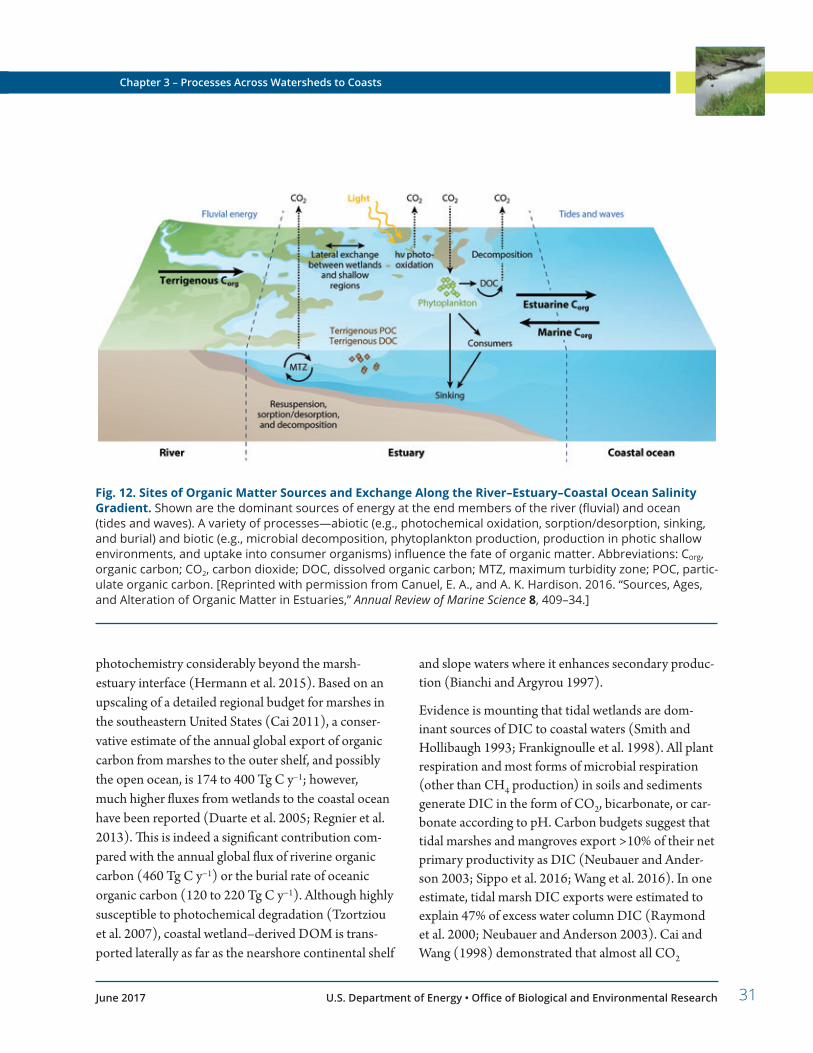
31



photochemistry considerably beyond the marsh- estuary interface (Hermann et al. 2015). Based on an upscaling of a detailed regional budget for marshes in the southeastern United States (Cai 2011), a conser-vative estimate of the annual global export of organic carbon from marshes to the outer shelf, and possibly the open ocean, is 174 to 400 Tg C y–1; however, much higher fluxes from wetlands to the coastal ocean have been reported (Duarte et al. 2005; Regnier et al. 2013). This is indeed a significant contribution com-pared with the annual global flux of riverine organic carbon (460 Tg C y−1) or the burial rate of oceanic organic carbon (120 to 220 Tg C y−1). Although highly susceptible to photochemical degradation (Tzortziou et al. 2007), coastal wetland–derived DOM is trans-ported laterally as far as the nearshore continental shelf

Fig. 12. Sites of Organic Matter Sources and Exchange Along the River–Estuary–Coastal Ocean Salinity Gradient. Shown are the dominant sources of energy at the end members of the river (fluvial) and ocean (tides and waves). A variety of processes—abiotic (e.g., photochemical oxidation, sorption/desorption, sinking, and burial) and biotic (e.g., microbial decomposition, phytoplankton production, production in photic shallow environments, and uptake into consumer organisms) influence the fate of organic matter. Abbreviations: Corg, organic carbon; CO2, carbon dioxide; DOC, dissolved organic carbon; MTZ, maximum turbidity zone; POC, partic-ulate organic carbon. [Reprinted with permission from Canuel, E. A., and A. K. Hardison. 2016. “Sources, Ages, and Alteration of Organic Matter in Estuaries,” Annual Review of Marine Science 8, 409–34.]

and slope waters where it enhances secondary produc-tion (Bianchi and Argyrou 1997).

Evidence is mounting that tidal wetlands are dom-inant sources of DIC to coastal waters (Smith and Hollibaugh 1993; Frankignoulle et al. 1998). All plant respiration and most forms of microbial respiration (other than CH4 production) in soils and sediments generate DIC in the form of CO2, bicarbonate, or car-bonate according to pH. Carbon budgets suggest that tidal marshes and mangroves export >10% of their net primary productivity as DIC (Neubauer and Ander-son 2003; Sippo et al. 2016; Wang et al. 2016). In one estimate, tidal marsh DIC exports were estimated to explain 47% of excess water column DIC (Raymond et al. 2000; Neubauer and Anderson 2003). Cai and Wang (1998) demonstrated that almost all CO2

32



degassing in the Satilla River estuary is supported by lateral carbon transport from intertidal salt marshes and that CO2 loss to the atmosphere exceeds the river DIC flux by tenfold.

Regular tidal flooding and sea level rise result in unusu-ally rapid rates of soil organic carbon sequestration and large carbon pools in tidal wetlands and seagrass beds compared to nontidal floodplain TAIs (Bridgham et al. 2006; Donato et al. 2011; Fourqurean et al. 2012). Although tidal wetlands occupy an area equivalent to just 2% of the ocean surface, they account for 50% of the carbon in marine soils and sediments (Mcleod et al. 2011; Hopkinson et al. 2012). Large-scale distur-bance of coastal wetlands contributes to climate forc-ing (Pendleton et al. 2012).

Hydrogeomorphic Processes at the Terrestrial-Aquatic Interface in Estuaries and CoastsHydrology is a master variable that regulates exchanges between terrestrial and aquatic systems across TAIs. Of particular importance is the two-way interaction between hydrology and geomorphology that shapes TAI ecology and biogeochemistry at all scales. While this perspective applies to all TAIs, it is arguably most important in estuaries and coasts where hydrology, geomorphology, and biology interact in ways that make TAIs highly dynamic over short temporal and spatial scales, ultimately determining the presence or absence of tidal wetlands.

Fig. 13. Conceptual Model of Coastal Carbon Cycling. This model includes tidal brackish and freshwater marshes, mangrove forests, saltwater marshes, and seagrass meadows and comprises estuaries and the coastal ocean. Abbreviations: CO2, carbon dioxide; DIC, dissolved inorganic carbon; DOC, dissolved organic carbon; POC, particulate organic carbon. [Image courtesy Jordan Barr. In: Troxler, T. G., et al. (in review). “Carbon Cycles in the Florida Coastal Everglades Socio-Ecological System Across Scales,” The Coastal Everglades: The Dynamics of Socio-Ecological Transformation in the South Florida Landscape. Eds. D. Childers, E. Gaiser, and L. Ogden.]

Terrestrial carbon input

Carbon export to open ocean

Surface deposition of organic carbon

Land-atmosphere, water-atmosphere CO2 exchange

Lateral transport of DIC, DOC, POC (includes estuary-ecosystem exchange and import/export between subdomains)

Biogeochemical cycling in the coastal zone

Aquatic deposition and burial of organic carbon

Tidal brackish and freshwater marshes

Mangrove forests and salt marshes

Seagrass meadows

Coastal oceans

33



The dynamics of an individual TAI are constrained by the geomorphic setting and vary considerably across estuaries, open coasts, barrier systems, and other large landforms, each of which adjusts to changes in the balance between wave energy (including long waves such as tides) and the distribution of sediment. Spatial and temporal variations in sed-iment supply, wave energy, tidal range, geomorphic setting (e.g., river delta, carbonate platform, and active margin), and historical rates of sea level rise largely control the distribution of inter-tidal and subtidal habitats. Ultimately, these variations also control carbon sequestration in coastal sediments, much of which is terrestrially derived (Blair and Aller 2012).

Vascular plants influence coastal hydro-geomorphology through feedbacks that stabilize them against long-term changes such as sea level rise and epi-sodic events such as storm surge erosion (see Fig. 14, this page). These feedbacks operate by two fundamentally different mechanisms that correspond to aboveground plant traits versus belowground traits. Sediment deposition on soil sur-faces increases in plant surface area, allowing plants to build elevation from the surface upward at rates that ultimately are limited by the local sediment supply (Kirwan and Megonigal 2013). Belowground plant production builds elevation from underneath the soil surface by depositing organic matter directly into the anaerobic soil profile where it is efficiently preserved compared to aboveground plant production. Below-ground production is critical to the stability of tidal wetlands where sea level rise is accelerating, because this production contributes about four times more elevation than an equal mass of inorganic sediment (i.e., silt or clay). However, microbial decomposition

causes SOM to be more prone to loss than inorganic sediment. As such, a critical need is to understand the biogeochemical conditions that regulate decomposi-tion in tidal wetland soils.

A large fraction (perhaps up to 10%) of plant- derived organic matter is recalcitrant to decay in the absence of oxygen, the overwhelming agent of preser-vation in saturated soils and sediments. The molecular composition of plant tissue is an important second-ary factor, but many mechanisms for organic matter preservation in uplands (Schmidt et al. 2011) are not important in wetlands. Organic matter preserved in marsh, mangrove, and seagrass soils is sensitive to changes in plant production (Mueller et al. 2016) and salinity (Craft 2007), among other factors.

Fig. 14. Ecohydrogeomorphic Feedbacks that Regulate Elevation Gain and Carbon Sequestration in Tidal Marshes. [Reprinted by permission from Macmillan Publishers Ltd.: Kirwan, L., and J. P. Megonigal. 2013. “Tidal Wetland Stability in the Face of Human Impacts and Sea-Level Rise,” Nature 504, 53–60. © 2013]

34



CHAPTER 4Drivers, Disturbance, and Extreme Events

36



Terrestrial-aquatic interface (TAI) systems, inherently dynamic in space and time, are subject to dramatic changes in structure and

function in response to external forcing. TAIs are often defined by events such as flooding that occur so regu-larly that they constitute a regime to which organisms are highly adapted and that cannot be interrupted without fundamentally changing the system. Other events are rare but critical for the long-term mainte-nance of ecosystem structure and function because they disrupt this short-term stability, thus maximizing long-term stability and creating a paradox in which the absence of disturbance makes the system vulnerable to degradation ( Johnstone et al. 2016). Finally, some disturbances are so dramatic that they directly degrade TAI systems (e.g., land-use change). As with terrestrial systems, carbon flux in TAIs following disturbances is expected to follow a conceptual trajectory with an immediate loss of carbon following a disturbance and subsequent recovery to either predisturbance carbon fixation rate or conversion to another ecosystem state. Carbon loss following disturbances such as fire, harvest removals, insect outbreaks, and coastal storms is the result of vegetation death, biomass combustion, and vegetation loss that alter primary productivity and eco-system respiration (Amiro et al. 2010). TAI systems also have very large soil carbon stocks that are suscep-tible to disturbances, particularly in peat-forming TAIs where plant production and slow, anaerobic decompo-sition are primary drivers of soil carbon accumulation (Pendleton et al. 2012). This section discusses the unique characteristics of TAIs that make them highly sensitive to external agents of change.

Drivers, Disturbance, and Extreme Events

Hydrologic DisturbanceTAIs are defined by characteristic hydrologic dynam-ics that give rise to hot spots and hot moments of bio-geochemical activity. As such, changes in hydrology are frequently the drivers of change in TAI systems. TAIs differ from other ecosystem types in that rela-tively subtle changes in hydrologic conditions cause dramatic impacts.

Climate-Driven Hydrologic ChangeChanging climate is a major agent of hydrologic change capable of altering TAI processes (Hulme 2005; Erwin 2008). Indeed, hydrology is a key reason that TAIs such as wetlands are among the ecosystems most vulnerable to climate change (Burkett and Kusler 2000; Winter 2000; Ferrati et al. 2005; Erwin 2008). Precipitation and evapotranspiration are important drivers of hydrology and thus soil carbon flux and soil organic carbon (SOC) content; soils tend to shift from net carbon uptake to carbon loss when condi-tions become drier. For example, the south Florida Everglades is a landscape-scale TAI system in which climate-driven changes in hydrology may have signifi-cant impacts (Obeysekera et al. 2011a). Some models project an annual increase in precipitation of up to 14% (IPCC 2013), but a decrease by up to 10% during the wet season (Christensen et al. 2007). This combi-nation of lower wet season and higher dry season pre-cipitation suggests overall less seasonality. However, uncertainties in model projections call for scenario- based approaches (Obeysekera et al. 2011b, 2015). Such climate-driven changes can result in broad-scale changes and feedbacks to plant community

4

37

Chapter 4 – Drivers, Disturbance, and Extreme Events



composition; primary production; and export of fresh-water, carbon, and nutrients to estuaries. Numerous examples exist that illustrate the profound influence of precipitation extremes on flood extent in wetland landscapes (i.e., Rouillard et al. 2015). However, the influence of flood extent resulting from drought and inundation events on wetland function varies signifi-cantly with wetland type and biogeochemical condi-tions, management history, and climate (Brigham et al. 1998; Venterink et al. 2002).

Changes in precipitation resulting in extreme events such as drought also have significant impacts on car-bon dioxide (CO2) exchange and carbon flux from soils. Drought can result in severe disturbance to peat-forming TAIs. Even short-duration drought can be conducive to accelerated rates of soil oxidation and decomposition at the exposed peat surface and can introduce the potential for peat fires. An El Niño event resulted in altered freshwater-marsh CO2 exchange rates with the atmosphere (Malone et al. 2014), a change consistent with experimental simulation of drought (Malone et al. 2013). Climate and environmental changes may increase the frequency or severity of drought events, and drought intensity was projected to result in wetlands converting to carbon sources across the United States (Chen et al. 2012). However, acute die-off has been attributed not only to drought-induced phenomena, but also to changes in soil chemistry, envi-ronmental pathogens, herbivory, and other stressors (McKee et al. 2004; Alber et al. 2008).

Changes in climate also are projected to result in larger convective storms and more intense hurricanes (Allan and Soden 2008). Hurricane disturbance results in significant CO2 flux to the atmosphere associated with defoliation, vegetation die-off, and increased exposure of soils to solar radiation; however, canopy structure and CO2 fluxes can recover fairly rapidly (Barr et al. 2012). When hydrologic patterns are altered, extreme storms can hinder recovery. In the coastal region of Louisiana, construction of flood-control levees, oil and gas canals, and roads through wetland areas have greatly altered hydrologic patterns over the past

hundred years, resulting in major changes to the natu-ral hydrologic regimes (Conner et al. 1981; Day et al. 2007). Sediment deposition has been altered and sub-sequent wetland accretion modified. In combination with regional land subsidence, these changes have led to increased flooding (Conner et al. 1993). The effects of hurricane disturbances in this region vary depend-ing on storm intensity and the extent of legacy hydro-logic alterations (Conner et al. 2014). Furthermore, in coastal marshes of southwest Florida, observed distur-bances from hurricanes and fire, along with saltwater intrusion, resulted in the conversion of peat marsh to open water (Wanless and Vlaswinkel 2005).

TAIs are highly sensitive to climate and environmen-tal changes that influence variability in temperature (Wint er 2000). Temperature extremes such as frosts and heat waves have contributed significantly to changes in TAIs, including the chilling damage observed in subtropical south Florida that resulted in major vegeta-tion die-off of mangrove trees (Ross et al. 2009). Also observed have been low-temperature events altering CO2 exchange with the atmosphere in subtropical TAIs (Malone et al. 2016). In coastal mangrove forests, the presence of hypersaline conditions and high solar irra-diance loading associated with climate variability can impose sharp reductions in carbon assimilation rates and suppress stomatal conductance (Barr et al. 2009), resulting in strong feedbacks with biogeochemical cycling and atmospheric CO2 emissions.

One of the most certain and severe consequences of a warming climate is the acceleration of sea level rise through land ice sheet melt and thermal expan-sion of ocean water (IPCC 2013). Accelerating sea level rise is a global perturbation affecting nearly all coastal TAIs. Water level relative to sediment surface is the dominant factor driving coastal zonation; thus, changes in water level will have dramatic impacts on coastal TAI boundaries in vertical and horizontal dimensions. Both tidal and coastal nontidal wetlands have some capacity for building vertically through soil development, thereby maintaining a constant elevation relative to sea level (Nyman et al. 2006;

38



McKee 2011; Lentz et al. 2016). However, this building is heavily dependent on hydrogeomorphic, biogeochemical, and productivity feedbacks that will be altered by climate and environmental changes. In particular, plant productivity and microbial processes respond to changes in inundation frequency, elevated CO2, and salinity, all of which can influence elevation gain or loss, as these processes exert feedbacks to soil elevation (Pezeshki et al. 1990; Cahoon et al. 2003). While small-scale models have begun to represent such processes and their influence on coastal eleva-tion dynamics, they have not yet been extrapolated to the global scale. There remain many uncertainties such as plant tolerance for flooding (Langley et al. 2013) and interactions with multiple climate change factors. Salt water intrusion can increase carbon loss from coastal TAIs by triggering a short-term reduc-tion in plant growth while stimulating heterotrophic respiration rates (Herbert et al. 2015).

Rising sea level can cause coastal wetlands to migrate horizontally onto uplands where conditions permit (Kirwan et al. 2016b). Many coastal areas at least have some capacity to adjust dynamically to rising seas. In some cases, coastal ecosystems can migrate hori-zontally, provided that inland landforms are suitable, and increase soil carbon stocks. For example, man-groves are migrating poleward to overtake marshes in subtropical regions all around the world because of declining freeze frequencies (Saintilan et al. 2014). Such a conversion from TAI herbaceous grasslands to TAI forests greatly increases carbon uptake on the landscape scale (Doughty et al. 2016). Coastal devel-opment can hinder the ability of these TAI ecosystems to migrate. The most obvious example is the hardening of shorelines by construction of concrete seawalls and jetties that commonly occurs along with dense coastal development. Currently, 14% of the U.S. coastline has been hardened, with a great likelihood of increasing future armament (Gittman et al. 2015). These struc-tures often preclude the horizontal migration of coastal wetlands, ultimately exacerbating coastal wetland loss.

Human Impacts on HydrologyTerrestrial-aquatic interfaces are highly sensitive to hydrologic modifications that increase their vulner-ability to other forms of disturbances (Nelson et al. 2008), with potential for nonlinear feedbacks and threshold exceedances (Herbert et al. 2015). Over a century of water management and hydrologic mod-ification in TAIs has dramatically altered wetlands across the United States, with the Florida Everglades being a prime example (Light and Dineen 1994; Davis et al. 2005). The construction of roads, canals, levees, and flow-control structures has modified the quantity, quality, timing, and location of water delivery to the Everglades. These changes have altered hydroperiods, salinity and nutrient levels, community assemblages, fire regimes, and ultimately carbon cycles and storage (Snyder and Davidson 1994; McCormick et al. 2001; Gaiser et al. 2006).

Agricultural drainage contributes to a persistent release of CO2 from TAIs previously under saturated condi-tions. Drainage can cause the loss of several meters of organic peat soil, depending on its depth (Hirano et al. 2012; Hooijer et al. 2012). To sustain agricultural production, drainage depth is continually drawn down, resulting in persistent carbon loss until soil carbon stocks are exhausted (Gleason and Stone 1994; McVoy et al. 2011). For example, Aich et al. (2013) and Hohner and Drecshel (2015) suggest that 7.6 to 9.2 × 108 megagrams of peat soil carbon have been lost from the Everglades Protection Area (i.e., the Everglades Agricultural Area Water Conservation Areas and parts of the freshwater Everglades National Park) over roughly the last 120 years. The increasing vulnerability of peatlands to combustion in response to drying and reduced precipitation in some regions exposed to cli-mate change and human activities likely will continue in coming decades (Turetsky et al. 2017). Human activities, which have concentrated in and around rivers and estuaries for millennia, have modified TAI processes through dredging, straightening, mining, and other uses (Nilsson et al. 2005). Moreover, river flow that generally prevents long residence times is

39



interrupted by reservoirs created for water manage-ment that trap sediment and organic matter and create enhanced methane (CH4) emissions (Guérin et al. 2006). Rapid expansion of hydropower in Asia and South America is adding reservoirs at an increasing pace. By altering processes in TAIs, human activities contribute to eutrophication and impacts from climate and environmental changes on aquatic systems, such as water column stratification, warming effects on metabolism, shifts in aquatic species distributions, and deoxygenation (Canuel et al. 2012).

Coastal zones constitute 2% of the world’s land area, but they contain 10% of the world’s population (600 million), 13% of the world’s urban population (360 million), and about 65% of the world’s cities with populations greater than 5 million (McGranahan et al. 2007). Typical human activities in the coastal zone cause changes in sediment dynamics, increased load-ing of nutrients to coastal wetlands, and conversion of coastal wetlands to open water and reclaimed land, with significant consequences for carbon sequestration and transport. Coastal wetlands, such as mangrove for-ests, tidal marshes, and seagrasses, comprise a TAI set that has been intensively modified by anthropogenic activities through hydrologic alterations such as drain-ing, filling, diking, and impoundment. Consequences of such activities include the rapid conversion of man-groves to shrimp ponds and fish farms through hydro-logic alteration, which leads to substantial carbon emissions to the atmosphere (Pendelton et al. 2012). Often the farms are abandoned after several years of cultivation because without plants to resist erosion and build soil, the ecosystem converts to open ocean with a subsequent loss of the carbon sequestration previ-ously provided by the mangrove forests. Ultimately, this process results not only in loss of forests, but also in loss of land area. Other practices drain tidal marshes for agriculture, dike them to separate marsh from tides, fill the area with imported sediment, and extract soil to construct ponds for salt production.

Estuarine aquatic systems are sensitive to disturbances. The effects of climate and environmental changes,

such as sea level rise and altered precipitation patterns, influence the hydrogeomorphic processes that regulate fluxes of freshwater, sediment, nutrients, and carbon (Najjar et al. 2010; Cloern et al. 2011). Cloern and Jassby (2012) identified six primary drivers of change in coastal-estuarine processes: water consumption and diversion, human modification of sediment sup-ply, introduction of nonnative species, sewage input, environmental policy, and environmental and climate shifts. Identifying universal trends across the systems is made difficult by the varying strengths of these drivers and their interactions across estuaries. Human popu-lation pressures near waterways and coastlines dictate that TAIs are necessarily susceptible to acute human disturbances that create or eliminate these systems (Donchyts et al. 2016). Coastal development remains the greatest threat to wetlands.

Accelerating sea level rise, along with other factors such as freshwater diversions, will shift the boundaries of tidal rivers, salinity regimes, the estuarine turbidity maximum, and the freshwater–brackish water interface in coastal aquifers. River diversion, channelization, and damming have cascading effects on the TAI continuum by altering sediment transport. If sediment is trapped behind dams, or allowed to flow directly into the ocean bottom, estuarine wetlands at the river mouths may become sediment starved and unable to maintain ele-vation. Deliberate alteration of hydrology also can be used to create wetlands.

Interactions of climate and human alterations of hydrology are difficult to predict. For example, drought is most commonly associated with reduced annual precipitation, but water-management challenges also can result in lower than desirable water levels with difficult-to-predict climate and environmental patterns. In 2010, El Niño conditions led to water levels that were well above average (Abtew et al. 2011) in the Florida Everglades, followed by higher than average discharges associated with water management. The following year, precipitation amounts lower than aver-age resulted in drought conditions with dry season water depths exceeding the lower tolerance for peat

40



conservation in Everglades freshwater marshes (Abtew et al. 2012; Sklar et al. 2012). Evident worldwide are climate and environmental impacts on the hydrol-ogy of large hydrologic basins, changing total rainfall amounts, extreme rainfall events and evapotranspira-tion, and interactions with human activities, along with subsequent and altered function of these large basins (Kuhn et al. 2011; Santos et al. 2014). These examples illustrate the sensitivity of TAIs to interactions of cli-mate and hydrology, uncertainties for how they vary by TAI type and setting, the degree of human impact, and feedbacks to environmental management with rel-evance at large spatial scales.

Disturbance of Organic-Rich SoilsTAI ecosystems such as tidal marshes, mangroves, seagrasses, nontidal floodplain forests, and nontidal peatlands are characteristically rich in soil carbon (i.e., Barr et al. 2010). These large carbon stocks are partic-ularly vulnerable to a variety of disturbances and can emit large amounts of CO2 and CH4 to the atmosphere (Pendleton et al. 2012). Climate warming is one driver capable of accelerating carbon loss from the vast stores in wetland soils. Soil carbon pools may be reduced by increased temperatures, changes in local water cycles, nutrient enrichment, changing lability of organic matter inputs, or combinations of these factors. Long-term SOC losses in terrestrial ecosystems with highly organic soils may have significant feedbacks on climate and environmental changes (Lashof and DeAngelo 1997). Comparably, wetlands hold massive stores of carbon that will continue to be susceptible to loss to the atmosphere, also resulting in significant climate feedbacks (e.g., Callaghan et al. 2004). However, recent experimentation with deep soil temperature manipu-lation has shown no stimulation of carbon loss even to extreme warming in a spruce forest peatland (Wilson et al. 2016). The anoxic and acidic conditions, along with low-quality organic matter in some TAI soils, may limit decomposition rates so severely that warming has no effect. However, this is a preliminary conclusion; warming effects on the stability of soil organic matter

stocks remain a major uncertainty in understanding TAI function in changing climates. Models will be use-ful for determining the extent to which soil warming may be decoupled from air warming in certain systems. For instance, oceanic influences could buffer tidal wet-land soil temperatures even as air temperatures rise.

Fire can emit large amounts of greenhouse gases from TAI systems because of their large soil carbon stocks, particularly peatlands and other systems with organic soils (Turetsky et al. 2014). Extensive SOC stocks fuel smoldering ground or subterranean fires that persist for days or weeks after the aboveground fire has passed. Not only does this extended duration of combustion allow for greater soil carbon loss, the combustion products from smoldering TAI fires pose amplified risks for both climate and environmental forcing and human health. Smoke from smoldering fires contain proportionately more pyrogenic carbon than flaming fires, particularly fine particulate matter and black carbon aerosols (Preston and Schmidt 2006). The impacts of TAI fires drew global attention during the severe 1997 and 2015 Indonesian fires, which caused widespread disruption of air travel and produced dan-gerous air quality conditions for extended durations. SOC stocks can change dramatically after disturbances affect plant primary productivity to reduce carbon inputs to peat-forming soils (Kirwan et al. 2009; Col-dren et al. 2016). For example, evidence from several coastal wetland studies shows that highly organic soils can subside or even collapse with saltwater intrusion. The dynamic feedback between plant production and soil microbial respiration that is altered by increasing concentration and duration of salt water and sulfate availability shifts the balance of soil carbon from gain to net loss. This phenomenon, also known as “peat col-lapse,” has been documented to varying degrees across the United States (Cahoon et al. 2003; Nyman et al. 2006; Voss et al. 2013). In coastal wetlands already exposed to disturbances such as saltwater intrusion or hydrologic drawdown, extreme climatic events (i.e., storms and drought) can change the state of TAIs.

CHAPTER 5Current State of Terrestrial-Aquatic Interface Modeling

42



One of the greatest challenges in effectively modeling terrestrial-aquatic interfaces (TAIs) is that they commonly fall in between tra-

ditional domains of existing process-based models. Furthermore, TAIs are isolated within the individual component models of Earth system models (ESMs) so that interactions between systems such as land and ocean or ocean and rivers are poorly captured or entirely absent. Models relevant to TAI processes were developed historically for needs that are (1) too spe-cific to a given terrestrial, wetland, or aquatic system; (2) too coarse in spatial and temporal resolution to capture hot spots and hot moments; or (3) missing fundamental processes important in TAIs. The impor-tance and value of advancing TAI-related science are that this development requires integration and coupling of existing models in new, robust ways. Fortunately, both understanding and modeling of traditional terres-trial and aquatic domains have advanced sufficiently to enable this next phase of model integration. TAIs provide a natural framework for integrating a suite of terrestrial, TAI, and aquatic processes into increasingly sophisticated models across a range of spatial and tem-poral scales to more robustly capture the occurrence and influence of hot spots and hot moments.

The following sections begin with an overview of ESMs and then discuss the existing state of TAI- relevant models—from high-resolution, process-rich, specialized models to capabilities currently in and being developed in ESMs. In the context of existing capabilities, the sections also highlight critical model deficiencies that must be addressed to overcome the scientific challenges that TAIs present.

Earth System ModelsESMs are intended to represent the global coupled dynamics of mass and energy transfer on model grids (at scales of tens of kilometers), including processes connecting land, atmosphere, ocean, and land and sea ice [see sidebar, Accelerated Climate Modeling for Energy (ACME), and Fig. 15, p. 43]. Current ESMs use land surface representations that explicitly resolve regions on the order of tens to hundreds of kilometers, which enable representations of continental-scale vari-ation connected to features such as major mountain ranges, coastal plains, and river drainages. The most sophisticated ESMs also include statistical represen-tations of finer variations in the land surface, known as subgrid representations. Current multilevel subgrid schemes capture land-surface variations in large cat-egories such as “natural vegetation,” “crop,” “glacier,” “urban,” or “lake.” Also captured are even finer details within some of these types, for example, the fraction of natural vegetation that each of a number of distinct plant types represents (e.g., trees versus shrubs versus grasses) or the fractional area of wetlands, bare soil, and rock. Proc esses are represented at multiple spatial scales within ESMs, dictated in part by the governing mecha-nisms, but also by current knowledge of processes and the ability to generalize process understanding. The model will encompass the enormous global diversity of physical and biological settings. ESMs currently include some simplistic representations of the proc esses neces-sary for a predictive understanding of TAIs and the role they play in structuring Earth’s climate.

An important limitation of current ESMs with respect to TAIs concerns extreme events, which are poorly

Current State of Terrestrial-Aquatic Interface Modeling

5

43

Chapter 5 – Current State of Terrestrial-Aquatic Interface Modeling



The Accelerated Climate Modeling for Energy (ACME) project is central to the U.S. Department of Energy’s (DOE) Earth System Modeling program under DOE’s Office of Biological and Environmental Research (BER). The Earth System Modeling program supports inno-vative Earth system model (ESM) capabilities, with the ultimate goal of providing accurate and computation-ally advanced representations of the fully coupled and integrated Earth system, as needed for energy and related sectoral infrastructure planning.

ESMs couple several component models that repre-sent individual elements of Earth’s climate system. Coupled ESM components—such as ACME’s Atmo-sphere, Ocean, Land, Sea Ice, and Land Ice—allow exchange of information such as moisture or heat among components. Launched by BER in 2014, the ACME project simulates the fully coupled Earth sys-tem at high resolution, incorporating coupling with energy, water, land-use, and energy- relevant activities.

In Fig. 15, overlapping regions of the ACME model represent model coupling. The Land and Ocean mod-els currently couple in a simple one-way export of river discharge into oceans, or directly to the ocean when land cells do not couple to a river (e.g., from ice sheets in Antarctica and Greenland). Additionally, in regions where a Land model grid cell is closer to the ocean, the model routes a river subsurface flow directly to the ocean. The model also will incorporate the ability to simulate the exchange of water to and from rivers and the surrounding landscape to repre-sent flooding along river corridors. Currently, ACME is in the early stages of developing coastal and estua-rine dynamics.

A fundamental attribute of ESMs is the discretization of each model component. ACME is developing atmo-sphere, ocean, and other Earth system simulation

components for use in Ocean, Sea Ice, and Land Ice models in the Model for Prediction Across Scales (MPAS) grid. This hexagonal MPAS grid enables regional variability in cell size to focus higher resolu-tion in areas of particular interest. The Atmosphere and Land models are using a cubed sphere, but ACME is moving its Land model to a watershed-based dis-cretization, as shown in the schematic above.

A major motivation for the ACME project is the par-adigm shift to come as computational capabilities move toward the exascale era. DOE, via its science programs, leadership computing centers, and early adoption of new computing architectures, tradition-ally leads many scientific communities, including Earth system simulation, through ongoing computing changes. The ACME collaborative project spans eight DOE national laboratories, four academic institutions, and one private company. For more information, see the ACME website (climatemodeling.science.energy.gov/projects/accelerated-climate-modeling-energy/).

Fig. 15. Accelerated Climate Modeling for Energy (ACME). ACME is an Earth system model supported by the U.S. Department of Energy. [Image courtesy Joel Rowland, Los Alamos National Laboratory]

Accelerated Climate Modeling for Energy

https://climatemodeling.science.energy.gov/projects/accelerated-climate-modeling-energy/

https://climatemodeling.science.energy.gov/projects/accelerated-climate-modeling-energy/

44



modeled in ESMs. In part, this lack of representation is due to the short temporal time frames in which TAI processes occur and to ESMs not containing sufficient resolution and detail of forcing features such as moun-tain ranges and coastal interfaces. While some work has identified where ESMs either perform well or are limited in terms of extremes (Sillmann et al. 2013a, b), this research area is still relatively young. There is a lack of observations of extremes in some cases, par-ticularly for precipitation events and high streamflow that threatens gauge stability. Models with variable resolution capabilities, such as the ACME Land Model (ALM), may be the best means to capture the fine temporal and spatial scales over which extreme events are carried out.

Terrestrial Hydrology and Reactive Transport ModelsJust as water is the backbone of TAIs, hydrology mod-els are the backbone of predictive models of TAIs. Capturing the water cycle is the critical first step in predicting any other aspect of TAIs, and nearly every aspect of TAIs is affected by and feeds back on the water cycle. Hydrology models are necessary tools to acquire data validation of processes at work in TAIs and to make predictions about system behavior. A hydrology model can be developed to capture the key hydrological processes that govern flow and transport of water, including dissolved constituents that may affect water quality. With a long history in U.S. Depart-ment of Energy applications, hydrology models have an exciting future. Described in this section are the existing and developing classes of hydrology models and the roles they play in TAI research.

Subsurface flow and reactive transport models, origi-nally intended for characterizing waste disposal sites and predicting the fate of contaminants, have long represented subsurface flow through physical solutions of mass conservation. These models use variably sat-urated formulations to predict soil moisture content as a function of time and space. Driven by this flow

solution, the chemical components of primary species are transported and reacted.

In many cases, models exist for individual processes, but gaps exist in the coupling of TAI-critical processes. This is particularly true at scales ranging from soil pores up to soil pedons. Modeling at these scales cap-tures soil characteristics such as surface tension and capillarity that regulate advective and diffusive solute transport. The models must represent grain boundar-ies and phase interfaces between mobile phases with extremely different viscosities and densities. Codes implementing the models must address these unique, process-driven challenges while simultaneously being computationally efficient and scalable enough to solve these problems on domains large enough to represent a continuum of grains. Although progress on these challenges has been made in the fields of secondary oil recovery and contaminant transport (Hassanizadeh and Gray 1993; Lichtner and Kang 2007), there is a need for fundamental research before such models are able to capture small-scale TAI phenomena that have large-scale implications.

Simultaneously, hydrology-specific models designed for the characterization and prediction of a watershed have been developed. Typically, hydrology models divide the watershed into (1) the land base on which precipitation falls, interacts with vegetation, and moves through or on soils and (2) the riverine environment, which governs the movement of water and nutrients down the channel and eventually into lakes or estua-rine environments. Land models generally are classed into “lumped” or “distributed,” and “deterministic” (process based) versus “stochastic.” The most relevant for understanding TAIs are distributed, process-based models (Condon and Maxwell 2015; Painter et al. 2016; Shen et al. 2016). These models use various formulations of subsurface and surface flow, along with many other sources and sinks of water (e.g., evapora-tion and transpiration) to determine the water balance for a particular land unit. They must include accurate descriptions of the watershed if they are to adequately perform and provide useful information such as on

45



rate, volume, and timing of flow and also include vegetation, soils, and topographic information (e.g., elevation, aspect, and slope).

At the ESM scale, the limited roles played by lateral flow and computational speed and capacity motivate a class of coarse-resolution models (i.e., at scales of one to hundreds of kilometers) based on columns. Vertical infiltration is solved on each subwatershed land sur-face, and lateral flow is characterized through overland routing models and base flow models. This runoff and base flow is then collected and passed to a riverine model (Clark et al. 2015). Given accurate inputs of surface weather over land (e.g., precipitation, tem-perature, humidity, incoming radiation, and winds), current global-scale and large-scale models can capture many of the large-scale features of observed water flow from major rivers into oceans, including the quantity and seasonal and interannual variations in flow timing (Zaitchik et al. 2010).

Current river routing models focus on the transport of liquid water (including, in some cases, ice). In development are explicit energy balance models that will allow prediction of stream temperatures across a range of scales from headwater streams to major rivers and over the full range of climate and environmental forcings from tropical rivers to ice sheet drainages (Li et al. 2015). These same modeling platforms also are being extended to include biogeochemical processes that influence the transformation of organic matter as it moves from headwater streams through river chan-nels and into estuaries. Energy and biogeochemistry components of river models also are being integrated with simulations of new physical processes that allow two-way interactions between land and stream via processes such as inundation (Clark et al. 2015). On the TAI land side, new aspects of the subgrid repre-sentation being introduced enable models to resolve the influences of varying elevations, terrain slopes, and aspects (e.g., compass orientation). Finally, the best current land models within ESMs also include signif-icant resolution of vertical connections (Tang et al. 2013; Tang and Riley 2016), called column dynamics,

within the soil. Vertical transports of energy, water, and organic matter are represented in layers extending many meters below the surface. This existing capability can facilitate simulation of groundwater interactions and connections between land and aquatic systems through the hyporheic zone.

Recent and ongoing efforts, enabled by increasing computational resources, are investigating a set of process-resolving, hyper-resolution models (HRMs; at scales of 10 meters to 1 kilometer) with three- dimensional (3D) flow. These models solve Richards’ equation in 3D, coupled through pressure and flux continuity to approximations of the shallow water equations for surface flow. Given the vast availability of these codes, there have been several extensive Model Intercomparison Project (MIP) efforts, which eluci-date the differences and similarities on both simple and more realistic simulations (Grenier et al. 2015; Kollet et al. 2017; Maxwell et al. 2014).

To capture water sources and sinks such as precipi-tation, evaporation, and transpiration, these models employ a wide variety of complexities—from parame-terizations to coupling existing column representations of vegetation and biogeochemistry and from global models to coupling process-resolving, scale-appro-priate models of vegetation. While the core of these models is hydrology, they also can have complex rep-resentations of canopy, litter and duff layers, root water uptake and plant hydraulics, and vegetation dynamics, and they could be coupled to state-of-the-art dynamic vegetation and biogeochemical models.

As HRMs become more mature, these model types promise to become subgrid components within coarse-resolution ESMs (i.e., upscaling) and to deter-mine to what degree HRMs influence climate and environmental characterizations at regional and local scales (i.e., downscaling). At the global scale, ESMs do not yet incorporate the hydrologic process under-standing that is well represented in HRMs, especially that of surface-groundwater interactions and extreme events. With the necessary finer-scale representations

46



of many climate and environmental characteristics—particularly in terms of water availability, timing, and quality as well as their resulting effects on human and engineered systems—these HRMs have much to offer. Their successful inclusion will require exascale com-puting resources and strategies such as asynchronous multitask parallelism. The localized nature of these subgrid models make them well suited to extreme par-allelism, but significant work remains.

Terrestrial Ecosystem ModelsThe wide variety of ecosystem-scale models can be broadly categorized as population models, demo-graphic or distribution models, and individual-based models (Porté and Bartelink 2002). Such models range in spatial scale levels from plant to stand to land-scape. Although superficially seeming to represent a broad range of diversity, most of these models tend to rely on very similar underlying principles and assump-tions (Hawkes 2000). Specifically, they tend to share many characteristics in their modeling of the abiotic and biotic system state, with discrete compartments tracking carbon and other elements, fixed time steps, and first-order soil carbon kinetics, and with a focus on aboveground plant production and biomass (for a counter example, see Grant 2015). Such models also have traditionally focused on forested ecosystems, a consequence of their origins as forestry yield tables (Pretzsch 1999) that were designed to assess the importance of forests in the global economy, climate, and carbon cycle (e.g., Hanewinkel et al. 2013).

Applying such models to mineral soil wetlands, peat-lands, and other terrestrial-aquatic systems is prob-lematic because these ecosystems have characteristics that are dominant in upland systems. These traits include high and fluctuating water tables, high-clay or organic soils (i.e., Histosols), significant methane (CH4) production and consumption, anoxic soil and low soil reduction-oxidation (redox) potentials, and the presence of productive bryophyte communities. These characteristics are all poorly treated by most upland models (Trettin et al. 2001). Indeed, terrestrial

model-data synthesis and comparison studies exhibit varied performances when run under fluctuating soil moisture conditions characteristic of wetlands and other TAI systems (Sulman et al. 2012; Zaehle et al. 2014; Keenan et al. 2012).

Efforts have been made to incorporate TAI-relevant processes into some upland models. For example, the addition of depth-explicit soil moisture, water storage, and nonvascular vegetation (i.e., bryophytes) to the Biome-BioGeochemical Cycles (BGC) model (Eng-strom and Hope 2011; Bond-Lamberty et al. 2007) or Photosynthetic/EvapoTransiration (PnET) model (Zhang et al. 2002), or fully prognostic water table cal-culations to the Community Land Model (CLM; Shi et al. 2015). These additions have improved the ability of models to accurately simulate TAI dynamics, but much remains to be done because effective simulation of such systems requires modeling anaerobic pathways; organic soil layers and peat deposits; vertical and hor-izontal water flow; and solute transport, soil oxygen-ation, and redox potential (Baird et al. 2009).

Dedicated wetland models incorporate many of the hydrological and biogeochemical complexities char-acteristic of TAIs. They can incorporate characteristics that are difficult to capture using traditional upland models, such as anaerobic biogeochemistry, deep organic-rich soils, dynamic soil surfaces that change elevation, shallow water tables, and plant species with novel morphology and ecophysiology (e.g., bryo-phytes). Because wetlands store massive quantities of carbon and exchange both carbon dioxide (CO2) and CH4 with the atmosphere, these ecosystems play an important role in the global carbon balance and potentially could accelerate global warming (Ringeval et al. 2011). Several recent regional and global wetland model-data comparison studies concluded that import-ant sources of uncertainty in model predictions of CO2 and CH4 emissions included (1) the seasonal effects of inundation on the position of the terrestrial- wetland interface, (2) representation of inundated plant processes such as gas transport through aeren-chyma, and (3) wetland subsurface biogeochemistry

47



(Bohn et al. 2015; Melton et al. 2013). The current ALM (version 1) has a representation of these proc-esses (Riley et al. 2011), as do other ESMs, but much work remains to ensure these models accurately predict greenhouse gas emissions under a changing climate (for a review, see Xu et al. 2016b). Missing components are, for example, tolerance for varying salinity condi-tions, interactions with anoxic environments typical in the shallow subsurface of many wetlands, and response to periodic inundation. A critical limitation of ESMs, and ecosystem models in general, arises because they typically conceptualize the landscape as individual, autonomous grid cells that exchange carbon and energy fluxes with the atmosphere but lack any cell-to-cell interaction or transport (McGuire et al. 2001). This simplification becomes untenable when modeling TAIs and highlights the need to couple these models with hydrology models capable of accurately predicting hydrologic fluxes across the landscape.

Estuarine ModelsRivers draining into coasts transition from freshwater systems with unidirectional flow to tidal freshwater rivers, to tidal saline rivers and estuaries that vary from oligohaline to fully saline. Although river estuaries form a natural TAI continuum, communities of scientists have traditionally isolated their research to either tidal or non-tidal portions of the continuum, and estuarine scientists have focused on saline reaches. Because tidal freshwater ecosystems are neither free flowing nor saline, there is a particular absence of research in these common TAIs. As a result, there is an urgent need to integrate terrestrial and riverine models with estuarine models.

Estuarine models are formulated to physically diagnose the hydrodynamics and transport resulting from strati-fied flows that arise from the exchange and interaction between saline ocean water and fresh riverine water. These models are designed to operate in the intertidal environment where periodic wetting and drying of nearshore tidal flats and marshlands are common. Example applications of estuarine modeling revolve around questions of tidal circulation and flushing,

coastline evolution (e.g., via sediment transport), ecosystem function (e.g., wetland restoration), and water quality modeling (e.g., the location of salinity, turbidity, or phytoplankton bloom fronts with respect to water intakes). Some estuarine models include bio-geochemical modules that simulate submerged aquatic vegetation, marshes, and sediment diagenesis, but these formulations are primitive and ignore processes such as export of solutes from soil porewater and ecosystem feedback capable of dynamically changing soil elevation.

The hydrodynamics in these models typically solves a simplified set based on the Reynolds-averaged Navier- Stokes (RANS) equation, which assumes flow is due primarily to tidal and meteorological forcing. Compo-nents involving assumptions of hydrostatic pressure and decoupling of horizontal and vertical turbulences ensure a vertical log-law profile and stability under hor-izontal shears (e.g., at a river confluence). Advanced models employ 3D RANS turbulence modeling and nonhydrostatic pressure. Ultimately, the fundamental challenge in estuarine modeling is obtaining the cor-rect datasets in bathymetry, shoreline geometry, forc-ing, biology, and validation, which often are sparse and incomplete. Forcing is particularly important in these systems because wind, waves, tides, and seasonal and episodic heating of the water can drive strong flows that occur in complicated geometries including bays, tidal river networks, and deltas. Input data required to build and validate an estuarine model include wind, waves, tides, turbulence, sediment transport, biogeo-chemistry, climatological data (e.g., solar forcing), bathymetry, and in situ observations via Acoustic Doppler Current Profilers, thermistor chains, and Lagrangian drifters. Typically, modeling occurs at 1 to 100 meters in spatial resolutions and temporal resolu-tions on the order of seconds; it is, therefore, unable to directly simulate turbulence, although modeling at finer scales is becoming more common.

There are two general classes of estuarine models: structured and unstructured grid models. Unstruc-tured grid models have gained popularity in the last decade, exhibiting the ability to represent complex

48



estuarine geometry better than traditional structured grid approaches. Premier unstructured grid models incorporate key processes that are needed to simulate fully coupled estuarine systems arising from flow, sediment, and ecological interactions. Models will vary in their numerics, but the state of the art typically includes generalized discretizations, especially in the vertical coordinate. Knowledge and varied applications of different numerical techniques that are appropri-ate to different physical geometries and forcing have evolved from multidecadal modeling efforts to diag-nose and apply best-practice numerics for estuarine modeling. Unlike the industry-standard Delft suite of models, unstructured research codes typically can be run in a high-performance computing context and are scalable to hundreds of processors.

Despite existing capabilities, this community lacks a MIP for evaluating different modeling systems inhib-iting adoption of a single model for use in arbitrary applications. To fully integrate land, river, and ocean modeling, these models should be able to seamlessly transition from 1D to 3D modeling, so that modeling of upstream rivers remains computationally inexpensive while still capable of resolving complex 3D flows within estuarine bays. This capability requires computation of 3D turbulence modeling and nonhydrostatic pressure.

Current ESMs do not capture estuarine processes or dynamics. These models represent the distribution of freshwater fluxes into ocean cells near river outlets. As river biogeochemistry advances, these flux compo-nents will become more sophisticated and enable sim-ulations of estuarine biogeochemistry. Recently, box models have been tested as a computationally efficient way to represent the influence of estuaries on the mix-ing and distribution of estuarine waters and chemistry with the open ocean (Tseng et al. 2016). The ability to locally increase spatial resolution in the ACME Model for Prediction Across Scales-Ocean (MPAS-O)

provides the potential to explicitly represent estuaries, although additional hydrodynamics will be needed to capture the influence of waves, tides, storm surges, and rising sea levels. Linking the ocean to the land in a way that enables the exchange of sediment and a changing coastline is an even greater challenge for accurate rep-resentation of coastal TAIs in ESMs.

Coastal Ecosystem ModelsThe stability and resilience of coastal ecosystems depend on the loss and gain of land related to rates of sea level rise and inundation. As discussed previously, this balance of land critically depends on the health and growth rate of vegetation within these ecosys-tems (see Fig. 10, p. 25). Recent efforts to quantify the trajectory of coastal ecosystems under land-use, climate, and environmental changes have sought to couple physical and biological (ecogeomorphic) processes in numerical models (Kakeh et al. 2016; Kirwan and Mudd 2012; Mudd et al. 2009; Swanson et al. 2014). These models incorporate above- and belowground plant growth, along with erosion and deposition of sediment in one dimension, to predict the gain and loss of land under a range of forcings and based on empirical data for plant dynamics for a variety of coastal species. Although these models rep-resent an important advancement in understanding and predicting the fate of coastal ecosystems, to date, this level of complexity in ecogeomorphic process feedbacks has yet to be incorporated into or coupled with physics-based models of estuarine dynamics and morphodynamics models that are used to predict the physical evolution of coastal settings via the use of hydrodynamics and sediment-transport equations. Incorporation of these models into ESMs will require advances in both ecogeomorphology and coastal ocean modeling as well as robust model coupling that enables dynamic interactions between land and ocean.

CHAPTER 6Critical Research Needs

50



Integration of Measurements, Modeling, and Experimentation

Generally, research approaches to investigating terrestrial-aquatic interface (TAI) ecosystems must lead to new understanding about the

role of these transitional ecosystems at the juncture of land and water in the Earth system, as well as the impacts of climate on the sensitive interfaces of ter-restrial and aquatic environments and ecosystems. Neither the three-dimensional (3D) spatial structures of these TAI ecosystems, nor the biophysical transfers and feedbacks of matter and energy throughout their structures, are currently well understood or modeled. Moreover, the net effect of transport processes through these ecosystems transforms their spatial structures, producing highly dynamic geomorphology and plant community structures. These dynamic structures, in turn, control aspects of element and water cycles. Thus, achieving fundamental new understanding about the role of TAI ecosystems on a global scale will require a research program that integrates mapping, measure-ment, and modeling. This chapter discusses these three approaches in more detail.

An observer of Earth’s terrestrial biomes naturally would conclude that TAI ecosystems are biologically diverse, just from recognizing the visible evidence of differences among temperate, tropical, and boreal forests, grasslands, and deserts. All biomes contain both terrestrial and aquatic ecosystems. Quantifying differences between them and identifying which have the most influence on element and water cycles are key challenges for a TAI research program to improve Earth system modeling. Whereas some of these

ecosystems may be large and relatively homogenous in function, and thus more easily characterized, others may be smaller and more heterogeneous yet still have large impacts. Prioritizing research accordingly to account for spatial heterogeneity in the area, volume, and elevation of wetlands at regional and global scales will help to save resources.

Careful integration of modeling with the collection of observational and experimental data will in large part determine the research program’s success. Given the likely importance of extreme events to these ecosys-tems, an understanding of such events and their effects is necessary to determine which are most character-istic of each biome. Similarly, knowledge of the most important drivers of key biophysical processes, such as reduction-oxidation geochemistry, is foundational to effective predictive modeling, as is an understanding of the scaling properties of biogeochemistry and trans-ferability among scales. Both extreme events and envi-ronmental drivers are also components of the risks and thresholds of ecosystem collapse related to the effects of climate and environmental changes.

The horizontal and vertical extent of TAI ecosystems has not been measured and thus is currently unknown, in part because of definitional challenges. Overcoming this issue is not a simple mapping problem. The inher-ent hydrodynamics and morphodynamics, which are essential elements of these systems, make developing standard practices necessary for measuring boundar-ies. These boundaries must incorporate disturbance regime factors such as the frequency, duration, and magnitude of inundation and their consequences for geomorphic structure within process domains. Thus,

Critical Research Needs6

51

Chapter 6 – Critical Research Needs



boundaries are not always visually discernible and are identifiable even less frequently through conventional remote-sensing techniques. A salient example of the challenges inherent in this type of mapping is flood-plain forested wetlands, whose canopies resist pene-tration by remotely operated sensors and contribute to the wetlands being easily confused with nonwetlands when there is no topographic and hydrologic data for modeling. The relevant methods for a 3D char-acterization will include integrated remote sensing, topographic mapping, and hydrologic modeling with change analysis of geomorphological features within process domains.

A key focus will be on measuring the fluxes, tempo-rary storage, and transformation of particulate and dissolved matter (e.g., organic and dissolved organic carbon) through TAIs such as riparian areas of head-water streams, river floodplains, and the littoral or inter-tidal zone along coasts. These efforts should include (1) measurements of partial pressure carbon dioxide (CO2) and oxygen fluxes, which are surprisingly sparse in the literature; (2) tracer studies of lateral and vertical transport to define the boundaries of process effects (e.g., Mulholland et al. 2008); (3) mesocosm studies (e.g., Jonsson et al. 2014); (4) biophysical-scale mod-els; and (5) experimental manipulations to elucidate the drivers of key ecosystem processes. Recognizing the need for plant and microbial studies is essential to assessing the factors that regulate biogeochemical transformations in TAIs. These factors include alloca-tion to roots and shoots by plants, biophysical transport of gases to root and stem tissues, and tissue nutrient concentrations. In some cases, such as tissue nutrient concentrations, measuring these features through remote sensing can support extrapolation to the global scale (e.g., Arrigo 2004; Malenovský et al. 2009).

Improving the understanding of TAI responses to extreme events is crucial to advancing knowledge of both the scale (temporal and spatial) of disturbances and the resulting interplay of their ecological and environmental feedbacks that interact at the scales of extreme-event phenomena. Field observations

and controlled experiments are important means to gather this information for inclusion in models. Also bolstering model-validation efforts will be improved observations of extreme precipitation, temperature that leads to changing patterns of runoff, and soil mois-ture and snowpack. Through improved understanding and representation of these events in models, scientists can examine the impacts of extremes on TAIs, such as drought and low flows. Without this information, knowledge of system stability and important inter-actions that may sustain or subdue TAI responses is incomplete and unclear.

The selection of study sites must meet multiple requirements and be conducted following the mining of open data available for TAI ecosystems both within and outside the United States. Workshop participants agreed on the need to address the primary research questions through a balance between long-term observations using sensors dispersed at broad spatial scales and “extensive” and “intensive” measurements of watersheds and smaller sites.

Multiscale ModelsA wide variety of ideas have been used and others proposed for advancing process understanding across scales, both up and down. Frequently, these ideas come to a choice between “embedding models” versus “embedding understanding”; both approaches can be appropriate for different systems. Embedded under-standing gives a name to a regularly used scientific approach—that is, simplifying physics while trying to maintain the essence of the details—a key strategy for all models. This process can be as simple as selecting effective parameters that average over subgrid hetero-geneity or, more effectively, developing empirical, subgrid models that capture the predictions of fine-scale, process-resolving models in a simplified form. Alternatively, users of embedded models strive to build fine-scale, process-resolving models directly, often in a stochastic or localized way. The technical and theo-retical challenges of this strategy can be quite difficult, and both can cause derailment. Technical challenges

52



include information passing and multilanguage compi-lation, and theoretical challenges include ensuring that the information passed between scales is both appro-priate and relevant. However, when chosen with care, both strategies can be extremely effective at capturing the essence of finer-scale processes in a coarser-scale model. These choices combine scientific intuition with formal mathematical methods; the resulting multiscale model must be evaluated carefully against observations at multiple scales.

Examples of embedding understanding are subgrid parameterizations, which are used extensively in global land models and intended to represent a spatially het-erogeneous or complex process in an averaged or sim-plified model. Examples of these subgrid parameters include water-retention models in hydrology, big-leaf vegetation models, and biogeochemical models. All have the advantage of being reasonably well under-stood, and many codes naturally enable the inclusion of new and improved parameterizations, making them easy to couple into existing coarser-scale mod-els. However, frequently in coupled systems, simple subgrid parameterizations do not sufficiently repre-sent the underlying physics, chemistry, or biology to address issues involving process interactions. In such cases, embedded models are necessary, and describ-ing uncertainty is imperative, based on assumptions invoked with the parameterizations. This requirement implies that creative and new approaches are desired (e.g., those that explore the application of scale-aware parameterizations, mesh-to-mesh interpolation, code-to-code data passing, and efficient use of computa-tional assets).

Alternatively, reduced-order models (ROMs) aim to run process-resolving models under a variety of con-ditions and then develop emulators or surfaces that fit model output as a function of a few key indicator variables. ROMs represent a promising strategy for sim-plifying the computational needs of subgrid, embed-ded models. However, these ROMs cannot be used in conditions outside the original training datasets. New research in dynamic ROMs and emulators that can be

continuously updated as the system changes between states and into no-analogue futures might remove some of these caveats.

The ongoing development of process-resolving models creates valuable research opportunities for multiscale Earth system models (ESMs). Most ESMs currently include some scale hierarchy that allows representation of multiple land types in a single grid cell. This arrange-ment provides the opportunity to insert subgrid mod-els, potentially in a spatially and temporally dynamic way, helping to address TAI characteristics as hot spots and hot moments. As episodic or extreme events occur, subgrid simulations of a process-resolving model can be spawned in an adaptive way. This strategy may be particularly relevant to TAIs, which fundamentally are below the resolution of a single ESM grid cell. Fur-thermore, embedding ensembles of runs within such a framework would provide the needed uncertainty esti-mates to inform impact assessments. These strategies necessarily would leverage exascale computing because their computational cost, while extremely expensive, would be highly parallelizable.

Because TAIs are characterized by their tight coupling of hydrology, geomorphology, ecology, and biogeochem-istry, modeling of these zones requires tackling a diverse landscape of existing legacy codes, new model and model- coupling developments, and uncertainty in process phys-ics. There is significant uncertainty in the structure of TAI models, not just in their parameters; thus, new efforts should be cognizant of this significant software challenge. Coupling state-of-the-art models across disciplines for TAIs demonstrates the need for a virtual ecosystem of software, with well-defined interfaces, built on advancing research in software frameworks for model structure exploration (e.g., Coon et al. 2016). In these cases, the metric for an efficient code often is measured in devel-oper time, not model run time. The development of new TAI models should leverage and extend new and emerg-ing technologies in interface design and functional multiphysics frameworks. These technologies should spur quick development and testing of new models and their coupling to existing models along with evaluation

53



against data and observations. Furthermore, these models and coupling must use modern software devel-opment best practices to ensure correctness and model accuracy despite the extreme complexity inherent in tightly coupled systems.

Multiscale Experiments and Their Integration with Predictive ModelsA major challenge is understanding how perturbations cascade up and down spatiotemporal scales to affect key TAI ecosystem functions. Gaining that mechanis-tic understanding outside observable system drivers and states requires going beyond single-scale obser-vations in natural settings via multiscale experimental manipulations. Multiscale experiments provide unique understanding on how processes play out across scales in these ecosystems. One reason is that the effect of a given perturbation likely depends on the scale of the system it is perturbing.

Although a broad range of studies likely could be con-ceptualized as a multiscale experiment, in this case the focus is on three classes of experiments that are not mutually exclusive. They include (1) direct manipu-lation of a system’s spatial scale, (2) manipulation of a larger-scale driver followed by tracking the responses of smaller-scale features, and (3) distributed networks of single-scale manipulations to link smaller-scale per-turbations to larger-scale phenomena.

Direct Manipulation of ScaleOne class of multiscale experiments invokes treat-ments that include direct manipulation of the spatial scale of the system being observed. This type of experiment might evaluate how the scale of an exper-imental system alters system function or response to perturbation. For example, Petersen et al. (2003) sum-marized coastal-zone experiments that manipulated the spatial scale of open water mesocosms. From these experiments, scaling relationships for primary produc-tion and zooplankton biomass were developed that applied to a larger-scale natural system (Chesapeake Bay). Importantly, Petersen et al. (2003) found that

experimentally derived scaling relationships did not apply for nitrogen recycling.

This finding highlights a key TAI knowledge gap—understanding which phenomena can and cannot be scaled or predicted from multiscale experiments. Phe-nomena that cannot be directly up-scaled will require particular attention in terms of understanding critical control-point mechanisms, including those that lead to scale transitions that occur at scales beyond those involved in manipulative experiments.

Knowledge of which features and processes can be represented as directly up-scaled parameters, and which cannot, is essential for efficiently coupling empirical data from multiscale experiments to pre-dictive multiscale models. In the earlier example, empirically derived scaling relationships for primary production and zooplankton biomass could be used to efficiently up-scale the small-scale observations as parameters for use in larger-scale simulations. In contrast, up-scaling the nitrogen recycling rate from small-scale experiments may require highly resolved (and computationally demanding) process models. Understanding when parameters can be empirically up-scaled versus when process models are required is a major challenge in TAI ecosystems due to their inher-ent multiscale organization.

Manipulation of Large-Scale DriversAnother class of multiscale experiments manipulates a larger-scale (e.g., landscape-scale) driver and studies the responses of smaller-scale system features and functions. This type of experiment also might make observations—in response to experimental perturbations—across a range of spatial and temporal scales. For example, Lan et al. (2015) experimentally evaluated the scale depen-dence of nitrogen-deposition impacts on plant species richness within a grassland system. The scientists defined a key nitrogen threshold in the system (referred to as Ncrit), which is the amount of nitrogen enrichment above which there is a significant decline in species richness (the number of species per area). Lan et al. (2015) found

54



that this threshold increased strongly with spatial scale. Thus, more nitrogen can be deposited in larger-scale systems before there is significant loss of species richness.

The Lan et al. (2015) study could be directly trans-lated to TAI ecosystems to examine how scale mod-ulates the nitrogen-deposition impacts (or other system-relevant perturbations) on biological diversity. A useful approach for such studies also would be to take a multitaxon or multimetric approach to examine shifts in species richness and functional trait diversity within plants, animals, and microorganisms that result from their combined influences over the functioning of TAI ecosystems.

Experiments that examine the scale dependence of drivers such as nitrogen deposition do not necessar-ily reveal underlying processes, but they do provide powerful constraints on multiscale models. That is, observed scale dependencies should be predictable from a multiscale model that faithfully represents key processes (see sidebar, Spruce and Peatland Responses Under Climatic and Environmental Change, and Fig. 16, p. 55). An inability to predict such scale tran-sitions may indicate structural deficiencies. In this case, additional experiment-model iterations would be needed to elucidate processes that cause observed scale dependencies. Such an approach, which ulti-mately will lead to improved process representation, is critical for robust predictions in TAI ecosystems because of the ongoing environmental changes that are pushing these systems beyond the environmental con-ditions used for model calibration.

Distributed Networks of Single-Scale ExperimentsDistributed networks of single-scale experimental manipulations can be conceptualized as a multiscale experiment that is used to understand how smaller- scale perturbations scale up to influence larger-scale phenomena. This type of experiment imposes a con-sistent set of perturbations and makes a consistent set of observations across a broad range of systems (e.g.,

across biomes). This design is multiscale in the sense that results can be aggregated at different spatial scales or across different environmental extents to examine the context dependence (and scale dependence) of perturbation impacts.

There are good examples of spatially distributed obser-vation networks [e.g., the National Ecological Obser-vatory Network (NEON) and AmeriFlux Network], but relatively few are broadly distributed manipulative experiments. One exciting exception is the Nutrient Network (NutNet), which has established equivalent nutrient-addition experiments in grassland ecosystems around the world. This approach has generated novel insights that could not be achieved using single-site experiments. For example, Stevens et al. (2015) showed that nitrogen deposition consistently increased annual net primary production in grassland systems, regardless of climate or other local conditions. This finding suggests that nitrogen deposition impacts on grasslands lack historical contingencies. On the other hand, O’Halloran et al. (2013) used NutNet data to reveal context dependencies in the relationship between primary production and decomposition rates.

Although distributed networks have been used in both terrestrial and aquatic ecosystems (Fraser et al. 2013), there is a need for distributed experiments to TAI ecosystems because of their very broad ranges of associated environmental conditions (e.g., coastal to freshwater and rainforests to deserts). For example, a network of sites that consistently imposes different levels of salt water intrusion on tidal freshwater sys-tems would significantly contribute to and advance the understanding of how sea level rise will impact these critical TAI ecosystems. Because such an approach combines controlled manipulations with cross-system observations, experimental outcomes can (1) provide empirical constraints—likely varying across systems—against which to calibrate and evaluate models and (2) reveal mechanisms that underlie observed context dependencies and, in turn, improve process represen-tation in predictive models.

55



Terrestrial-aquatic interface (TAI) ecosystems such as peatlands, tidal marshes, mangroves, and non-tidal wetlands accumulate large soil carbon pools. These carbon stocks may be vulnerable to acceler-ated decomposition when disturbed by drainage, erosion, and climate change. Peatlands cover only 3% of Earth’s land surface but contain about 30% of the global soil carbon pool. The Spruce and Peat-land Responses Under Climatic and Environmental Change (SPRUCE) project is an experiment that simu-lates the response of northern peatland ecosystems to higher atmospheric carbon dioxide (CO2) concen-trations and temperature. Led by Oak Ridge National Laboratory, the SPRUCE experiment is assessing a decade of responses to these perturbations across multiple scales of ecological organization, including microbial communities, moss populations, vascular plant species, and some insect groups. To identify and quantify these critical environmental response mechanisms, the Terrestrial Ecosystem Science pro-gram within the U.S. Department of Energy’s (DOE) Office of Biological and Environmental Research sup-ports this whole-ecosystem experiment in northern Minnesota (see Fig. 16). SPRUCE provides a platform for testing mechanisms controlling the vulnerability of organisms, biogeochemical processes, and ecosys-tem functions to important environmental change variables. Examples are thresholds across which pop-ulations increase or decline, limitations to regenera-tion, biogeochemical limitations to productivity, and the cycling and release of CO2 and methane.

The SPRUCE project connects observations to new modeling approaches for improved climate predic-tions, incorporating the complex relationships among warming, drying, microbial processes, and vegeta-tion responses associated with climatic change. This comprehensive suite of spruce-dominated peatland

process studies and observations accelerates model development by improving the representation of proc esses, model calibration, and model validation for boreal systems. Insights come from both small-scale processes and landscape-relevant water, carbon, and energy fluxes for similar peatlands. SPRUCE is a coop-erative joint venture by scientists from DOE national laboratories, the U.S. Department of Agriculture’s Forest Service, and universities. For more information, see the SPRUCE website (mnspruce.ornl.gov).

Spruce and Peatland Responses Under Climatic and Environmental Change

Fig. 16. Spruce and Peatland Responses Under Climatic and Environmental Change (SPRUCE) Project Site. Interior of a SPRUCE open-topped warming enclosure showing natural snow accumula-tion during a mid-winter precipitation event in Minne-sota. [Image courtesy Oak Ridge National Laboratory]

56



Watershed ApproachesQuantification and predictive modeling of coupled hydrological and biological processes within intercon-nected hydrological systems necessitate a distributed network of observational sites spanning a diversity of ecosystems in multiple regions, climates, and land uses. While such a network of sites already exists within federally supported programs, these sites are focused only marginally on assessing process-level connectivity among ecosystems, often treating each as a unique feature of the landscape. Surprisingly lacking are studies seeking to bridge multiple sites spanning a broad continuum from headwaters to coastlines via an interconnected observational and modeling frame-work. In contrast, a coordinated research program designed to integrate research activities and assimilate observational, experimental, and modeling efforts across the current constellation of field study sites within the United States is warranted both to enhance multi agency collaborative efforts and to advance the state of the science. Examples include the U.S. Depart-ment of Energy’s (DOE) Next-Generation Ecosystem Experiments and Scientific Focus Area field sites, the National Science Foundation’s Critical Zone Obser-vatories and NEON, and the National Oceanic and Atmospheric Administration’s National Estuarine Research Reserve System. Research activities within DOE’s Climate and Environmental Sciences Division in the Office of Biological and Environmental Research have emphasized data-model integration as a guiding principle for quantifying and predicting ecosystem behavior and its response to episodic and multidecadal climate drivers leading to extreme events. Moreover, numerous DOE field studies supplement purely obser-vational data with those derived from experimental manipulation of key environmental states, such as tem-perature and soil moisture, to resolve mechanistic- and process-level behavior. These data can be embedded within ESMs, which are used subsequently to identify gaps in proc ess understanding and to guide future experimental activities (Covino 2016).

To elucidate the role that TAIs play in regulating the flow of water and nutrients within interconnected

hydrological systems along the “summit-to-seas” con-tinuum, the critical research need posited for achieving this goal is to develop an interconnected, coordinated network of field observatories. Placing a network of observatories within a unifying modeling context is well aligned with existing DOE research activities in both the Terrestrial Ecosystem Science and Subsurface Biogeochemical Research programs. Recognizing that key ecosystems may be underrepresented within the existing national network of observatories (e.g., coastal zone environments), these programs may require addi-tional resources to expand and develop observational capabilities in such areas. The use of a unifying ESM (or models) enables bridging of scales and study sites in a manner that largely obviates the need for a continuous chain of sites along a single interconnected hydrological system. Data-model integration activities are coordi-nated and expected to identify key system components and compartments within the network, along with key environmental parameters that must be measured in a consistent manner from site to site to constrain and cali-brate models and validate their predictions.

Given the diversity of TAI systems identified in this workshop report that exert critical controls on water and nutrient export, only a broad network of field study sites appears capable of capturing the level of process information needed to populate predictive models describing their behavior. Building on and expanding where needed the existing distributed net-work of field observatories and assimilating the key data types derived from each of them into predictive models describing TAI processes represent the most feasible means to make rapid progress in this research area. Additionally, the legacy of preexisting data made available through direct engagement of the network of observatories is expected to greatly expedite the process of data assimilation within predictive models describing TAI phenomena. Focusing on a single site or sites that fail to account for the diversity of systems identified in this report would limit broad research relevance and applicability across scales important to quantifying the role of such systems in regulating continental- to global-scale water, carbon, and nutrient budgets.

CHAPTER 7Summary and Priorities

58



The critical terrestrial-aquatic interface (TAI) is not characterized by geographic location; it is defined by physical interactions that drive key-

stone processes. In contrast to recent perception, this interface is not merely a conduit through which solu-ble and particulate materials are exchanged between soils and water bodies. Instead, it is biogeochemically dynamic, transforming the materials that flow through the system, and interactive with the broader domain in which it is embedded. Characterizing these TAIs are steep process gradients in spatially compressed zones, and the current limited understanding of these process dynamics often is inferred only by comparing measurements of fluxes into and out of the interfaces. This limited knowledge is a large source of uncertainty in global and regional models of carbon, environment, and climate, also significantly impeding the ability to couple models across traditional process and research domains in meaningful and robust ways. Because these interfaces are ubiquitously distributed globally, a fun-damental understanding of the hallmark processes in TAIs is needed to extend site-specific observations to a more globally relevant knowledgebase. Gathering this data will enable integration of models across process domains, spanning spatial and temporal scales. For these reasons, TAI-focused research is a priority of the scientific community, both to advance the science and to improve the predictability of the Earth system.

Several identified research challenges will focus these efforts:

■ Global Accounting of TAI Distribution, State, and Stores of Carbon and Nutrients: A Scaling Challenge. Despite the known importance of

Summary and Priorities

TAIs, there is (1) a lack of an accurate accounting of the location, size, and element inventory of TAI systems and (2) a basic but fundamental research need for an accurate global accounting of TAI carbon and nutrient stocks, fluxes, and transforma-tions, which is a critical gap in representing these systems in models. The challenge applies across all types of TAIs and is critical to assessing the extent to which these diverse ecosystems currently serve as net sources or sinks of carbon and how they will respond to changing anthropogenic releases of car-bon and future alterations to climate, environment, and land use. Experience dictates that the challenge of scaling TAI processes from fine-scale phenomena to robust regional, continental, and global inven-tories will require creative new ways of integrating plot-scale, process-based research; landscape-scale, geospatially explicit databases; remote sensing; process-based numerical modeling; and creative new scaling concepts.

■ Coupling Processes Across Traditional Eco-system Boundaries: A Transdisciplinary Chal-lenge. Traditionally, terrestrial, aquatic, and TAI ecosystems and processes have been the focus of separate scientific communities. This separation was due in part to the fact that many ecological and biogeochemical phenomena operate at different scales across systems, making quantification of their processes logistically and conceptually dif-ficult. Similar challenges apply to the coupling of models that were designed to operate separately for terrestrial, TAI, or aquatic systems. Understanding processes across terrestrial-TAI-aquatic boundaries

7

59

Chapter 7 – Summary and Priorities


Chapter 7 – Summary and Priorities

also is fundamentally a challenge of scale. Processes that operate at small scales of time and space in TAIs drive large-scale phenomena that cannot be predicted with existing observational or model-ing techniques. Advancing TAI science requires creative approaches to combining experiments, models, and observations that respect (rather than ignore) inherent differences in scale. Achieving this vision will require the development of scientific teams willing to work across traditional ecosystem boundaries and a cooperation across agencies that generally tend to focus funding on separate and different elements of the terrestrial-TAI-aquatic continuum.

■ Advancing a Predictive Understanding of Cou-pled Biogeochemical Cycles Through Improved Integration of Hydrologic, Geomorphic, Plant, and Microbial Processes. Tremendous progress has been made over the past decades in under-standing the biogeochemical feedbacks from biological and physical agents of change, including plants, microorganisms, hydrology, and geomor-phology. This process-based understanding has advanced interactively through a combination of improved small- and large-scale observations, experimental manipulation, and numerical mod-eling. The result has been an improved capacity to understand and forecast change as illustrated by the increasing sophistication of Earth system models (ESMs), and TAIs represent the next big challenge in this evolution. Capturing crucial TAI processes in ESMs (and other models), requires bold new efforts to further integrate hydrology, plant biology, microbial ecology, and geomorphology in an Earth system context. Such efforts will need to account for (1) interactions between surface and ground-water as they move through TAI plant communi-ties and soils; (2) changes in landscape structure

resulting from sediment loss and gain; (3) the relationships between physiological and morpho-logical plant traits and their responses to changes in oxygen availability, salinity, sediment deposition, warming, and other sources of plant stress; and (4) factors that regulate microbial community composition and microbial activities as they relate to reduction-oxidation potential and environmen-tal gradients, including microbial processes in the plant rhizosphere.

■ Ecological and Biogeochemical Responses to Perturbations and Feedbacks on System Resil-ience. Ecological and biogeochemical feedbacks tend to maintain ecosystems in a state of quasi equilibrium and, thereby, persist in landscapes for long periods of time. However, dramatic pertur-bations can exceed the capacity of ecosystems to recover and can lead to state changes (e.g., wet-land to aquatic). A challenge for TAI science is to understand the features and processes that render ecosystems more or less resilient to spatial or tem-poral changes in external drivers such as hydrology, land use, climate, or sediment loads. Perturbations to such drivers arising from floods, droughts, fire, or sea level rise can affect TAIs both directly and indirectly via the terrestrial and aquatic systems to which they are coupled. Thus again, the challenge of scale is apparent because some perturbations occur at regular intervals (e.g., spring tide flood-ing) while other cases occur infrequently (e.g., hurricanes and wildfires). Clearly, the dynamics of human systems will need to be considered because of the immensity of their effects on key physical and biological processes. Understanding and pre-dicting the impacts of perturbations (large and small) on TAIs require focusing on scale-relevant research and modeling.

60



APPENDICESAppendix 1: Federal Interagency Coordination and Collaboration ......................63

Appendix 2: Agenda ..........................................65

Appendix 3: Workshop Breakout Questions ..67

Appendix 4: Workshop Participants ...............69

Appendix 5: References ....................................73

62


Terrestrial-Aquatic Interfaces

63


A Vision for Addressing Gaps in Terrestrial-Aquatic Interface Research

The findings discussed in this report from the September 2016 Research Priorities to Incorporate Terrestrial-Aquatic Interfaces

in Earth System Models Workshop clearly indicate that the terrestrial-aquatic interface (TAI) is a critical, complex system with important implications for nat-ural and human processes and process interactions. The findings also demonstrate that gaps in current knowledge of TAIs are impeding the ability to predict the responses and feedbacks of these critical ecosys-tems to environmental changes and disturbances (e.g., land use, fire, and floods). Because improving the confidence in predictions involves an approach that combines model development with observations and field experiments, the prediction framework must be robust over all appropriate temporal and spatial scales. As such, advancing the state of the science of TAI ecosystems should employ approaches that directly feed and improve predictive models—an ambitious and urgent scientific grand challenge. This challenge to advance TAI science demands the application and integration of numerous scientific disciplines includ-ing biology, ecology, hydrology, modeling, sociology, chemistry, meteorology, and oceanography. Develop-ing a predictive understanding of this complex system also requires careful integration and coupling of these disciplines and represents a unique opportunity to coordinate basic research among the scientific and fed-eral research communities in ways that lead to positive outcomes for society.

The U.S. Department of Energy (DOE) has a long his-tory of tackling grand challenges such as TAI research through large-scale field experiments [e.g., Free-Air CO2 (carbon dioxide) Enrichment (FACE), Integrated Field Research Challenge, and Next-Generation Eco-system Experiments], long-term observation campaigns

Appendix 1: Federal Interagency Coordination and Collaboration

(e.g., Atmospheric Radiation Measurement program and AmeriFlux Network), and complex efforts to model coupled Earth systems [e.g., Accelerated Climate Modeling for Energy (ACME)]. To address critical questions at the interface of energy and environment, DOE makes significant research investments in areas such as terrestrial ecosystems, subsurface biogeochem-istry, Earth system modeling, genomics, and atmo-spheric science. However, the breadth and integrative nature of TAIs require a diversity of scientific disci-plines that goes beyond those that involve only DOE.

The larger federal research community currently sup-ports numerous activities that complement or inter-face with the transdisciplinary nature of TAI science, including the following examples.

■ DOE and the U.S. Forest Service collaborate in providing support to the Spruce and Peatland Responses Under Climatic and Environmental Change Experiment (SPRUCE). SPRUCE is a decade-long experiment investigating the role played by artificially warmed air and soils on peat-land carbon dynamics.

■ The Smithsonian Institution operates the Global Change Research Wetland, a field facility ded-icated to integrated, long-term (i.e., 30-year) manipulative experiments, observations, and modeling of carbon cycling in a coastal tidal marsh. Observations, remote sensing, and ecosystem-scale numerical models advance fore-casts of impacts on coastal wetland processes of rising CO2, nitrogen enrichment, invasive species, sea level rise, and warming.

■ The National Science Foundation supports a num-ber of Long-Term Ecological Research (LTER) sites that include TAIs such as the Plum Island Ecosys-tems LTER and the Virginia Coast Reserve LTER, as well as various Critical Zone Observatories and

Appendix 1: Federal Interagency Coordination and Collaboration

64



future National Ecological Observatory Network sites that examine watershed-scale science.

■ The U.S. Geological Survey has long supported a national stream gage network and has demon-strated growing interests in wetlands and studies of blue carbon.

■ The U.S. Department of Agriculture has made numerous investments to understand ecosystem services provided by wetland and coastal systems as well as wetland mitigation practices relevant to agricultural systems.

■ The National Aeronautics and Space Administra-tion’s Earth Sciences Division has demonstrated expertise in understanding ocean and aquatic bio-geochemistry impacted by land processes observed from airborne and satellite platforms.

■ The National Oceanic and Atmospheric Admin-istration’s National Estuarine Research Reserve System, as well as related coastal and ocean carbon programs, has focused on understanding the aquatic carbon cycle.

■ Applied research and policy programs at the U.S. Department of Defense (e.g., Strategic Environmen-tal Research and Development Program and U.S. Army Corps of Engineers) have focused on mitigat-ing and regulating the impacts of disturbance events such as floods along rivers and the coastal margin.

This list is not exhaustive, but it does demonstrate a broad level of federally supported research seeking to understand and manage the interface between land and water.

Given this rich body of support for TAI science, opportunities exist whereby coordination across

federal institutions could increase the scientific return of overall national investments. Robust understanding of the transdisciplinary, complex systems that include TAIs benefits tremendously from strategic coordina-tion of, and collaborations involving, numerous federal agencies and stakeholders. With carefully coordinated research agendas, these complementary investments and objectives can decrease the time needed to achieve scientific breakthroughs and at the same time reduce unnecessary overlap and long development periods for new capabilities. The congressionally mandated U.S. Global Change Research Program provides an ideal example and venue where federal agencies interact, strategize, and implement coordinated research efforts that combine the interests and expertise of multiple federal research programs to tackle grand scientific challenges such as TAI research.

Although the TAI workshop focused on DOE and its specific mission, this report highlights a broader opportunity to coordinate future research efforts among multiple federal agencies and stakeholders. Recent workshops and meetings sponsored by federal and academic programs on, for example, TAIs, blue carbon, coastal ecosystems, ocean biogeochemistry, and wetlands have come to the same conclusion—the understanding of TAIs represents a significant gap in knowledge of the coupled Earth system. Careful col-laborations across multiple agencies will enable the coordination of investments while reducing unneces-sary duplication of effort and preserving each agency’s mission areas. Ultimately, this will result in a robust and comprehensive understanding of, and predictive capability for, TAIs that will be useful both to advance the science and to provide important information to stakeholders and policymakers for making informed decisions that involve these complex ecosystems.

65


Appendix 2: AgendaResearch Priorities to Incorporate Terrestrial-Aquatic Interfaces

in Earth System Models WorkshopSeptember 7–9, 2016

Hilton Washington, D.C./Rockville Hotel1750 Rockville Pike, Rockville, MD 20852

Day 1: Wednesday, September 7

7:30–9:00 a.m. Breakfast9:00–9:40 a.m. Welcome and Introductory Comments (Eisenhower Room) 9:00 a.m.–9:05 a.m. Welcome J. DeForest 9:05 a.m.–9:15 a.m. Climate and Environmental Sciences Division G. Geernaert Interest in Terrestrial-Aquatic Interfaces (TAIs) 9:15 a.m.–9:20 a.m. Role of Workshop Reports D. Stover 9:20 a.m.–9:30 a.m. Scope and Workshop Charge J. DeForest

9:30 a.m.–9:40 a.m. Breakout Logistics and Initial Questions and Answers J. DeForest, Workshop Organizers9:40–10:10 a.m. Plenary Sessions (Eisenhower Room) 9:40 a.m.–9:50 a.m. An Overview of TAIs P. Megonigal 9:50 a.m.–10:20 a.m. Current State and Needs of TAI Modeling R. Leung, W. Riley, P. Thornton 10:20 a.m.–10:30 a.m. Geomorphology and Landscape Dynamics J. Rowland 10:30 a.m.–10:40 a.m. Ecosystem Carbon Cycling in TAIs P. Raymond 10:40 a.m.–10:50 a.m. Major Disturbance in TAIs T. Troxler10:50 a.m.–11:00 a.m. Break11:00 a.m.–1:15 p.m. Breakout Sessions11:00 a.m.–1:00 p.m. Breakout Session Topic 1: Physical Processes Group A: (Monroe Room) Lead: V. Bailey Rapporteur: E. Coon Group B: ( Jackson Room) Lead: J. Rowland Rapporteur: P. Raymond Group C: (Lincoln Room) Lead: P. Megonigal Rapporteur: H. Diefenderfer1:00 p.m.–1:15 p.m. Summarizing Group Discussion for Rapporteurs1:15 p.m.–2:15 p.m. Working Lunch and Interaction Time (Lobby, Eisenhower Room)1:45 p.m.–2:15 p.m. Breakout Session Reporting (Eisenhower Room)2:15 p.m.–4:30 p.m. Breakout Sessions1:45 p.m.–4:15 p.m. Breakout Session 2: Spatial and Temporal Heterogeneity Group A: (Monroe Room) Lead: T. Troxler Rapporteur: E. Canuel Group B: ( Jackson Room) Lead: J. Rowland Rapporteur: P. Thornton Group C: (Lincoln Room) Lead: P. Megonigal Rapporteur: A. Langley4:15 p.m.–4:30 p.m. Summarizing Group Discussion for Rapporteurs4:30 p.m.–4:45 p.m. Break4:45 p.m.–5:15 p.m. Breakout Session Reporting (Eisenhower Room)5:15 p.m.–5:45 p.m. Open Discussion (Eisenhower Room)5:45 p.m. Summary and Closing (Eisenhower Room) Workshop Organizers6:00 p.m. Collaboration of Writing Teams Selected Members

Appendix 2: Agenda

66



Day 2: Thursday, September 8

7:30 a.m.–9:00 a.m. Breakfast9:00 a.m.–9:10 a.m. Welcome and Reconvening Comments (Eisenhower Room) 9:00 a.m.–9:10 a.m. Welcome and Comments Workshop Organizers9:10–9:50 a.m. Plenary Session (Eisenhower Room) 9:10 a.m.–9:20 a.m. Research Opportunities at the Critical Zone Observatories W. McDowell 9:20 a.m.–9:30 a.m. Microbial Controls on Biogeochemical Processes in TAIs K. Wrighton 9:30 a.m.–9:40 a.m. Fine-Scale Processes V. Bailey 9:40 a.m.–9:50 a.m. Process Scaling from Fine to Landscape Scales S. Fendorf10:00 a.m.–12:15 p.m. Breakout Sessions10:00 a.m.–12:15 p.m. Breakout Session 3: Biogeochemical and Ecological Processes Group A: (Monroe Room) Lead: V. Bailey Rapporteur: S. Fendorf Group B: ( Jackson Room) Lead: T. Troxler Rapporteur: M. Mayes Group C: (Lincoln Room) Lead: P. Megonigal Rapporteur: M. Newcomer12:00 p.m.–12:15 p.m. Summarizing Group Discussion for Rapporteurs12:15 p.m.–1:15 p.m. Lunch12:45 p.m.–1:15 p.m. Breakout Session Reporting (Eisenhower Room)1:15 p.m.–4:00 p.m. Breakout Sessions1:15 p.m.–3:30 p.m. Breakout Session 4: Future Directions Group A: (Monroe Room) Lead: V. Bailey Rapporteur: B. Benscotter Group B: ( Jackson Room) Lead: T. Troxler Rapporteur: J. Stegen Group C: (Lincoln Room) Lead: J. Rowland Rapporteur: A. Langley3:15 p.m.–3:30 p.m. Summarizing Group Discussion for Rapporteurs3:30 p.m.–4:00 p.m. Breakout Session Reporting (Eisenhower Room)4:00 p.m.–4:15 p.m. Break4:15 p.m.–4:45 p.m. Open Discussion (Eisenhower Room) Workshop Organizers4:45 p.m.–5:15 p.m. Synthesizing the Major Themes (Eisenhower Room) Workshop Organizers5:15 p.m.–5:30 p.m. Summary and Closing (Eisenhower Room) Workshop Organizers5:30 p.m. Collaboration of Writing Teams Selected Members

Writing Day: Friday, September 9

67


Day One

1. Physical Processes

a. Which physical processes and dynamics are most important to capture in models designed to forecast changes in TAIs? In the coupling between TAIs and adjacent systems?

b. What are the thresholds at which changes in hydrol-ogy, sediment dynamics, sea level, land-use change, or other physical drivers force TAIs across biogeochemi-cal or ecological thresholds to cause state change?

c. Given DOE’s aim to improve the performance of Earth system models (ESMs), which TAIs, or proc esses that may unify TAIs, are most poorly understood? Why? Which TAIs do models most poorly represent?

d. Which model structures and modeling gaps must be prioritized to capture key spatial and temporal scales that regulate TAI physical processes?

2. Spatial and Temporal Heterogeneity

a. Which disturbances, perturbations, or climatic extreme events in TAIs, both in space and time, most fundamentally alter TAI function?

b. How can scientists recognize and quantify system thresholds, particularly when they operate across large spatial and temporal scales that require exper-tise across disciplines such as hydrological and ecosystem-climate feedbacks?

c. What is the current state of models in terms of capturing relevant spatial and temporal variabilities,

especially as these differences relate to disturbances or perturbations?

d. What are the critical needs for improving multiscale observations and modeling in TAIs to improve the understanding of their spatial and temporal heterogeneities?

Day Two

3. Biogeochemical and Ecological Processes

a. What are the dominant controls on changes in plant traits, plant community dynamics, and plant ecophys-iologies in TAIs, especially those that are relevant to ecosystem function, ecosystem-climate feedbacks, and ESMs?

b. Which properties of microbial communities and which of their processes are relevant to the key biogeo-chemical processes that distinguish TAI ecosystems?

c. What are the thresholds at which biological, biogeo-chemical, ecological, and ecosystem dynamics lead to system-relevant state changes?

d. Which model structures and modeling gaps must be prioritized to capture the relevant spatial and tempo-ral scales that regulate biological and biogeochemi-cal processes of TAIs?

4. Future Directions

a. Which human activities fundamentally affect the relevant physical, biological, and biogeochemical processes in TAIs? Which of them are most relevant for the biogeochemical coupling of TAIs to adjacent ecosystems or Earth systems?

Appendix 3: Workshop Breakout Questions

The purpose of the breakout sessions is to determine the state of the science and the most important and pressing research priorities that would lead to significant improvements to a predictive understanding of terrestrial-aquatic interfaces (TAIs) in the context of climate and environmental forcings. Importantly, the U.S. Department of Energy (DOE) is interested in discovery science that strengthens models by bridging gaps in the process-level understanding of phenomena that drive changes in the Earth system.

Appendix 3: Workshop Breakout Questions

68



b. What are the biggest challenges to linking TAI- relevant physical and biological processes in terms of both observations and modeling?

c. What combination of observations, experiments, and facilities are needed to parameterize multiscale

models to improve the predictive understanding of TAIs in the Earth system?

d. What topics did we miss?

69


Appendix 4: Workshop Participants

Co-ChairsVanessa Bailey Pacific Northwest National Laboratory

Patrick Megonigal Smithsonian Environmental Research Center

Joel Rowland Los Alamos National Laboratory

Tiffany Troxler Florida International University

ParticipantsKatrina Bennett Lawrence Livermore National Laboratory

Brian Benscoter Florida Atlantic University

Brian Bergamaschi U.S. Geological Survey

Ben Bond-Lamberty Joint Global Change Research Institute, Pacific Northwest National Laboratory

Nicholas Bouskill Lawrence Berkeley National Laboratory

Scott Bridgham University of Oregon

Amy Burgin University of Kansas

Elizabeth Canuel Virginia Institute of Marine Science

Ethan Coon Los Alamos National Laboratory

David Lesmes Program Manager, Climate and Environmental Sciences Division

Fig. 17. Workshop Participants. Participants of the Research Priorities to Incorporate Terrestrial-Aquatic Inter-faces in Earth System Models Workshop.


70



Heida Diefenderfer Pacific Northwest National Laboratory

Scott Fendorf Stanford University

Charlotte Grossiord Los Alamos National Laboratory

Christine Hawkes University of Texas, Austin

Valerie Ivanov University of Michigan

Sujay Kaushal University of Maryland

Ken Kemner Argonne National Laboratory

Randall Kolka U.S. Forest Service

Kevin Kroger U.S. Geological Survey

Adam Langley Villanova University

Ruby Leung Northwest National Laboratory

Melanie Mayes Oak Ridge National Laboratory

William McDowell University of New Hampshire

Whitman Miller Smithsonian Environmental Research Center

Umakant Mishra Argonne National Laboratory

Raymond Najjar Pennsylvania State University

Rebecca Neumann University of Washington

Michelle Newcomer Lawrence Berkeley National Laboratory

Christopher Osburn North Carolina State University

Peter Raymond Yale University

Daniel Ricciuto Oak Ridge National Laboratory

William Riley Lawrence Berkeley National Laboratory

James Stegen Pacific Northwest National Laboratory

Jinyun Tang Lawrence Berkeley National Laboratory

Peter Thornton Oak Ridge National Laboratory

Maria Tzortziou City University of New York

Kenneth Williams Lawrence Berkeley National Laboratory

Kelly Wrighton Ohio State University

U.S. Department of Energy Office of Biological and Environmental ResearchSharlene Weatherwax Associate Director for Science

Gary Geernaert Director, Climate and Environmental Sciences Division

Paul Bayer Program Manager, Climate and Environmental Sciences Division

Jared DeForest Program Manager, Climate and Environmental Sciences Division

Andrew Flatness Scientific Program Specialist, Climate and Environmental Science Division

Renu Joseph Program Manager, Climate and Environmental Sciences Division

Dorothy Koch Program Manager, Climate and Environmental Sciences Division

71


Sally McFarlane Program Manager, Climate and Environmental Sciences Division

Rickey Petty Program Manager, Climate and Environmental Sciences Division

Daniel Stover Program Manager, Climate and Environmental Sciences Division

Robert Vallario Program Manager, Climate and Environmental Sciences Division

Tristram West Senior Technical Advisor

ObserversNancy Cavallaro U.S. Department of Agriculture, National Institute of Food and Agriculture

Dwight Gledhill National Oceanographic and Atmospheric Administration

Kathy Hibbard National Aeronautics and Space Administration

Laura Lorenzoni National Aeronautics and Space Administration

Hank Margolis National Aeronautics and Space Administration

Karina Schaefer National Science Foundation

Gyami Shrestha U.S. Carbon Cycle Science Program Office

Zhiliang Zhu U.S. Geological Survey


72



73


Appendix 5: References

Abril, G., et al. 1999. “Oxic/Anoxic Oscillations and Organic Carbon Mineralization in an Estuarine Maximum Turbidity Zone (The Gironde, France),” Limnology and Oceanography 44(5), 1304–15. DOI:10.4319/lo.1999.44.5.1304.

Abtew, W., et al. 2012. “Chapter 2: Regional Hydrology.” In South Florida Environmental Report, 1–38. Ed. G. Redfield. South Florida Water Management District, West Palm Beach.

Abtew, W., et al. 2011. “Pan Evaporation and Potential Evapo-transpiration Trends in South Florida,” Hydrological Processes 25(6), 958–69. DOI:10.1002/hyp.7887.

Aich, S., et al. 2013. “Estimating Soil Subsidence and Carbon Loss in the Everglades Agricultural Area, Florida Using Geospa-tial Techniques,” Agriculture, Ecosystems & Environment 171, 124–33. DOI:10.1016/j.agee.2013.03.017.

Alber, M., et al. 2008. “Salt Marsh Dieback: An Overview of Recent Events in the U.S.,” Estuarine, Coastal and Shelf Sci-ence 80(1), 1–11. DOI:10.1016/j.ecss.2008.08.009.

Algora, C., et al. 2013. “Geochemistry and Microbial Popu-lations in Sediments of the Northern Baffin Bay, Arctic,” Geomicrobiology Journal 30(8), 690–705. DOI:10.1080/ 01490451.2012.758195.

Allan, R. P., and B. J. Soden. 2008. “Atmospheric Warming and the Amplification of Precipitation Extremes,” Science 321(5895), 1481–84. DOI:10.1126/science.1160787.

Amiro, B. D., et al. 2010. “Ecosystem Carbon Dioxide Fluxes After Disturbance in Forests of North America,” Journal of Geophysical Research: Biogeosciences 115(G4), G00K02. DOI:10.1029/2010jg001390.

Angelini, C., et al. 2011. “Interactions Among Foundation Spe-cies and Their Consequences for Community Organization, Biodiversity, and Conservation,” BioScience 61(10), 782–89. DOI:10.1525/bio.2011.61.10.8.

Arai, H., et al. 2016. “Function of the Methanogenic Commu-nity in Mangrove Soils as Influenced by the Chemical Prop-erties of the Hydrosphere,” Soil Science and Plant Nutrition 62(2), 150–63. DOI:10.1080/00380768.2016.1165598.

Armstrong, J., and W. Armstrong. 2001. “Rice and Phragmites: Effects of Organic Acids on Growth, Root Permeability, and Radial Oxygen Loss to the Rhizosphere,” American Journal of Botany 88(8), 1359–70. DOI:10.2307/3558443.

Arora, B., et al. 2016. “Influence of Hydrological, Biogeochemical and Temperature Transients on Subsurface Carbon Fluxes in a Flood Plain Environment,” Biogeochemistry 127(2), 367–96. DOI:10.1007/s10533-016-0186-8.

Arrigo, K. R. 2004. “Marine Microorganisms and Global Nutrient Cycles,” Nature 437, 349–55. DOI:10.1038/nature04159.

Baird, A. J., et al. 2009. “Upscaling of Peatland-Atmosphere Fluxes of Methane: Small-Scale Heterogeneity in Process Rates and the Pitfalls of “Bucket-and-Slab” Models.” In Car-bon Cycling in Northern Peatlands, 37–53. Eds. A. J. Baird et al. American Geophysical Union, Washington, D.C. DOI:10.1029/2008GM000826.

Barr, J. G., et al. 2012. “Hurricane Disturbance and Recovery of Energy Balance, CO2 Fluxes and Canopy Structure in a Mangrove Forest of the Florida Everglades,” Agricul-tural and Forest Meteorology 153, 54–66. DOI:10.1016/j.agrformet.2011.07.022.

Barr, J. G., et al. 2010. “Controls on Mangrove Forest-Atmo-sphere Carbon Dioxide Exchanges in Western Everglades National Park,” Journal of Geophysical Research: Biogeosciences 115(G2), G02020. DOI:10.1029/2009jg001186.

Barr, J. G., et al. 2009. “Physiological Responses of Red Man-groves to the Climate in the Florida Everglades,” Journal of Geophysical Research: Biogeosciences 114(G2), G02008. DOI:10.1029/2008jg000843.

Bennett, E. M., et al. 2001. “Human Impact on Erodable Phos-phorus and Eutrophication: A Global Perspective,” BioScience 51(3), 227–34.

Benscoter, B. W., et al. 2015. “Wildfire as a Key Determinant of Peatland Microtopography,” Canadian Journal of Forest Research 45(8), 1132–36. DOI:10.1139/cjfr-2015-0028.

Berner, R. A. 1994. “GEOCARB II: A Revised Model of Atmo-spheric CO2 over Phanerozoic Time,” American Journal of Science 294(1), 56–91. DOI:10.2475/ajs.294.1.56.

Bethke, C. M., et al. 2011. “The Thermodynamic Ladder in Geomicrobiology,” American Journal of Science 311(3), 183–210. DOI:10.2475/03.2011.01.

Bianchi, T. S. 2006. Biogeochemistry of Estuaries. Oxford University Press, New York.

Bianchi, T. S., and M. E. Argyrou. 1997. “Temporal and Spatial Dynamics of Particulate Organic Carbon in the Lake Pontchar-train Estuary, Southeast Louisiana, U.S.A,” Estuarine, Coastal and Shelf Science 45(5), 557–69. DOI:10.1006/ecss.1997.0237.

Blair, N. E., and R. C. Aller. 2012. “The Fate of Terrestrial Organic Carbon in the Marine Environment,” Annual Review of Marine Science 4, 401–23. DOI:10.1146/annurev-marine-120709-142717.


74


Bohn, T. J., et al. 2015. “WETCHIMP-WSL: Intercomparison of Wetland Methane Emissions Models over West Siberia,” European Geosciences Union: Biogeosciences 12, 3321–49. DOI:10.5194/bg-12-3321-2015.

Bond-Lamberty, B., et al. 2007. “Improved Simulation of Poorly Drained Forests Using Biome-BGC,” Tree Physiology 27(5), 703–15. DOI: 10.1093/treephys/27.5.703.

Borges, A. V., et al. 2005. “Budgeting Sinks and Sources of CO2 in the Coastal Ocean: Diversity of Ecosystems Counts,” Geophysical Research letters 32(14), L14601. DOI:10.1029/2005gl023053.

Börner, K., et al. 2010. “A Multi-Level Systems Perspective for the Science of Team Science,” Science Translational Medicine 2(49), 49cm24. DOI:10.1126/scitranslmed.3001399.

Bridgham, S. D., et al. 2006. “The Carbon Balance of North Ameri-can Wetlands,” Wetlands 26(4), 889–916. DOI:10.1672/0277-5212(2006)26[889:tcbona]2.0.co;2.

Bridgham, S. D., et al. 1998. “Carbon, Nitrgen, and Phosphorus Mineralization in Nortern Wetlands,” Ecology 79(5), 1545–61. DOI:10.1890/0012-9658(1998)079[1545:cnapmi]2.0.co;2.

Brinson, M. M. 1993. “Changes in the Functioning of Wetlands Along Environmental Gradients,” Wetlands 13(2), 65–74. DOI:10.1007/bf03160866.

Bromham, L., et al. 2016. “Interdisciplinary Research Has Consistently Lower Funding Success,” Nature 534(7609), 684–87. DOI:10.1038/nature18315.

Broussard, W., and R. E. Turner. 2009. “A Century of Changing Land-Use and Water-Quality Relationships in the Conti-nental US,” Frontiers in Ecology and the Environment 7(6), 302–07. DOI:10.1890/080085.

Brown, R. R., et al. 2015. “Interdisciplinarity: How to Catalyse Collaboration,” Nature 525, 315–17. DOI:10.1038/525315a.

Bullock, A. L., et al. 2013. “Anaerobic Metabolism in Tidal Freshwater Wetlands: III. Temperature Regulation of Iron Cycling,” Estuaries and Coasts 36(3), 482–90. DOI:10.1007/s12237-012-9536-5.

Bunn, S. E., and A. H. Arthington. 2002. “Basic Principles and Ecological Consequences of Altered Flow Regimes for Aquatic Biodiversity,” Environmental Management 30(4), 492–507. DOI:10.1007/s00267-002-2737-0.

Burgin, A. J., and S. K. Hamilton. 2007. “Have We Over-emphasized the Role of Denitrification in Aquatic Ecosystems? A Review of Nitrate Removal Pathways,” Frontiers in Ecology and the Environment 5(2), 89–96. DOI:10.1890/1540-9295(2007)5[89:hwotro]2.0.co;2.

Burkett, V., and J. Kusler. 2000. “Climate Change: Potential Impacts and Interactions in Wetlands of the United States,” JAWRA Journal of the American Water Resources Association 36(2), 313–20. DOI:10.1111/j.1752-1688.2000.tb04270.x.

Cahoon, D. R., et al. 2003. “Mass Tree Mortality Leads to Mangrove Peat Collapse at Bay Islands, Honduras After Hurricane Mitch,” Journal of Ecology 91(6), 1093–105. DOI:10.1046/j.1365-2745.2003.00841.x.

Cai, W.-J. 2011. “Estuarine and Coastal Ocean Carbon Para-dox: CO2 Sinks or Sites of Terrestrial Carbon Incineration?” Annual Review of Marine Science 3, 123–45. DOI:10.1146/annurev-marine-120709-142723.

Cai, W.-J., and Y. Wang. 1998. “The Chemistry, Fluxes, and Sources of Carbon Dioxide in the Estuarine Waters of the Satilla and Altamaha Rivers, Georgia,” Limnology and Ocean-ography 43(4), 657–68. DOI:10.4319/lo.1998.43.4.0657.

Cai, Y., et al. 2013. “Effects of Tropical Cyclones on River Chem-istry: A Case Study of the Lower Pearl River During Hurri-canes Gustav and Ike,” Estuarine, Coastal and Shelf Science 129, 180–88. DOI:10.1016/j.ecss.2013.05.019.

Callaghan, T. V., et al. 2004. “Effects of Changes in Climate on Landscape and Regional Processes, and Feedbacks to the Cli-mate System,” AMBIO: A Journal of the Human Environment 33(7), 459–68. DOI:10.1579/0044-7447-33.7.459.

Camporeale, C., et al. 2013. “Modeling the Interactions Between River Morphodynamics and Riparian Vegetation,” Reviews of Geophysics 51(3), 379–414. DOI:10.1002/rog.20014.

Canuel, E. A., and A. K. Hardison. 2016. “Sources, Ages, and Alteration of Organic Matter in Estuaries,” Annual Review of Marine Science 8, 409–34. DOI:10.1146/annurev-marine-122414-034058.

Canuel, E. A., et al. 2012. “Climate Change Impacts on the Organic Carbon Cycle at the Land-Ocean Interface,” Annual Review of Earth and Planetary Sciences 40, 685–711. DOI:10.1146/annurev-earth-042711-105511.

Castañeda-Moya, E., et al. 2010. “Sediment and Nutrient Depo-sition Associated with Hurricane Wilma in Mangroves of the Florida Coastal Everglades,” Estuaries and Coasts 33(1), 45–58. DOI:10.1007/s12237-009-9242-0.

Chambers, L. G., et al. 2016. “Effects of Salinity and Inundation on Microbial Community Structure and Function in a Man-grove Peat Soil,” Wetlands 36(2), 361–71. DOI:10.1007/s13157-016-0745-8.

Chambers, L. G., et al. 2011. “Short-Term Response of Carbon Cycling to Salinity Pulses in a Freshwater Wetland,” Soil Science Society of America 75(5), 2000–07. DOI:10.2136/sssaj2011.0026.


75


Chen, G., et al. 2012. “Drought in the Southern United States over the 20th Century: Variability and Its Impacts on Terres-trial Ecosystem Productivity and Carbon Storage,” Climatic Change 114(2), 379–97. DOI:10.1007/s10584-012-0410-z.

Childers D. L, et al. 2000: “Twenty More Years of Marsh Estuarine Flux Studies: Revisiting Nixon (1980).” In Concepts and Con-troversies in Tidal Marsh Ecology, 391–423. Eds. M. P. Weinstein and D. A. Kreeger. Kluwer Academic Publishers, Dordrecht, Netherlands.

Christensen, J. H. 2007. “Regional Climate Projections.” In Climate Change 2007: The Physical Science Basis. Contribution of Working Group I to the Fourth Assessment Report of the Intergovernmental Panel on Climate Change. Chapter 11, Cambridge University Press, Cambridge, United Kingdom, and New York.

Clark, M. P., et al. 2015. “Improving the Representation of Hydro-logic Processes in Earth System Models,” Water Resources Research 51(8), 5929–56. DOI:10.1002/2015wr017096.

Cloern, J. E., and A. D. Jassby. 2012. “Drivers of Change in Estuarine- Coastal Ecosystems: Discoveries from Four Decades of Study in San Francisco Bay,” Reviews of Geophysics 50(4), RG4001. DOI:10.1029/2012rg000397.

Cloern, J. E., et al. 2011. “Projected Evolution of California’s San Francisco Bay-Delta-River System in a Century of Climate Change,” PLOS ONE 6(9), e24465. DOI:10.1371/journal.pone.0024465.

Coldren, G. A., et al. 2016. “Chronic Warming Stimulates Growth of Marsh Grasses More Than Mangroves in a Coastal Wetland Ecotone,” Ecology 97(11), 3167–75. DOI:10.1002/ecy.1539.

Cole, J. J., et al. 2007. “Plumbing the Global Carbon Cycle: Integrating Inland Waters into the Terrestrial Carbon Budget,” Ecosystems 10(1), 172–85. DOI:10.1007/s10021-006-9013-8.

Condon, L. E., and R. M. Maxwell. 2015. “Evaluating the Rela-tionship Between Topography and Groundwater Using Outputs from a Continental-Scale Integrated Hydrol-ogy Model,” Water Resources Research 51(8), 6602–21. DOI:10.1002/2014WR016774.

Conner, W. H., et al. 2014. “Impacts of Changing Hydrology and Hurricanes on Forest Structure and Growth Along a Flooding/Elevation Gradient in a South Louisiana Forested Wetland from 1986 to 2009,” Wetlands 34(4), 803–14. DOI:10.1007/s13157-014-0543-0.

Conner, W. H., et al. 1993. “Bottomland Hardwood Produc-tivity: Case Study in a Rapidly Subsiding, Louisiana, USA, Watershed,” Wetlands Ecology and Management 2(4), 189–97. DOI:10.1007/bf00188153.

Conner, W. H., et al. 1981. “Comparison of the Vegetation of Three Louisiana Swamp Sites with Different Flooding Regimes,” American Journal of Botany 68(3), 320–31. DOI:10.2307/2442768.

Coon, E. T., et al. 2016. “Managing Complexity in Simulations of Land Surface and Near-Surface Processes,” Environ-mental Modelling & Software 78, 134–49. DOI:10.1016/j.envsoft.2015.12.017.

Covino, T. 2017. “Hydrologic Connectivity as a Framework for Understanding Biogeochemical Flux Through Watersheds and Along Fluvial Networks,” Geomorphology 227, 133–44. DOI:10.1016/j.geomorph.2016.09.030.

Craft, C. 2007. “Freshwater Input Structures Soil Properties, Verti-cal Accretion, and Nutrient Accumulation of Georgia and U.S. Tidal Marshes,” Limnology and Oceanography 52(3), 1220–30. DOI:10.4319/lo.2007.52.3.1220.

Dahm, C. N., et al. 2015. “Extreme Water Quality Degradation Following a Catastrophic Forest Fire,” Freshwater Biology 60(12), 2584–99. DOI:10.1111/fwb.12548.

Darke, A. K., and J. P. Megonigal. 2003. “Control of Sediment Deposition Rates in Two Mid-Atlantic Coast Tidal Freshwa-ter Wetlands,” Estuarine, Coastal and Shelf Science 57(1–2), 255–68. DOI:10.1016/s0272-7714(02)00353-0.

Davis, S. M., et al. 2005. “A Conceptual Model of Ecological Inter-actions in the Mangrove Estuaries of the Florida Everglades,” Wetlands 25, 832–42. DOI:10.1672/0277-5212(2005)025 [0832:acmoei]2.0.co;2.

Day, G., et al. 2008a. “The Depositional Web on the Flood-plain of the Fly River, Papua New Guinea,” Journal of Geophysical Research: Earth Surface 113(F1), F01S02. DOI:10.1029/2006jf000622.

Day, G., et al. 2008b. “Chapter 3 The Rapid Spread of Mine- Derived Sediment Across the Middle Fly River Floodplain,” Developments in Earth and Environmental Sciences 9, 113–52. DOI:10.1016/s1571-9197(08)00403-5.

Day, R. H., et al. 2007. “Chapter 2 - Hydrology of Tidal Fresh-water Forested Wetlands of the Southeastern United States.” In Ecology of Tidal Freshwater Forested Wetlands of the Southeastern United States, 29–63. Eds. W. H. Conner, T. W. Doyle, and K. W. Krauss. Springer, The Netherlands. DOI:10.1007/978-1-4020-5095-4_2.

Donato, D. C., et al. 2011. “Mangroves Among the Most Carbon-Rich Forests in the Tropics,” Nature Geoscience 4, 293–97. DOI:10.1038/ngeo1123.

Donchyts, G., et al. 2016. “Earth’s Surface Water Change over the Past 30 Years,” Nature Climate Change 6, 810–13. DOI:10.1038/nclimate3111.

Doughty, C. L., et al. 2016. “Mangrove Range Expansion Rapidly Increases Coastal Wetland Carbon Storage,” Estuaries and Coasts 39(2), 385–96. DOI:10.1007/s12237-015-9993-8.

Doyle, T., et al. 1995. “Wind Damage Effects of Hurricane Andrew on Mangrove Communities Along the Southwest Coast of Florida, USA,” Journal of Coastal Research 21, 159–68.


76


Duarte, C. M., et al. 2005. “Major Role of Marine Vegetation on the Oceanic Carbon Cycle,” European Geosciences Union: Biogeosciences 2(1), 1–8. DOI:10.5194/bg-2-1-2005.

Dunne, T., et al. 1998. “Exchanges of Sediment Between the Flood Plain and Channel of the Amazon River in Brazil,” Geological Society of America Bulletin 110(4), 450–67. DOI:10.1130/ 0016-7606(1998)110<0450:EOSBTF>2.3.Co;2.

Emerson, D., et al. 2013. “Anaerobic Metabolism in Tidal Fresh-water Wetlands: II. Effects of Plant Removal on Archaeal Microbial Communities,” Estuaries and Coasts 36(3), 471–81. DOI:10.1007/s12237-012-9496-9.

Engstrom, R., and A. Hope. 2011. “Parameter Sensitivity of the Arctic Biome–BGC Model for Estimating Evapotranspira-tion in the Arctic Coastal Plain,” Arctic, Antarctic, and Alpine Research 43(3), 380–88. DOI:10.1657/1938-4246-43.3.380.

Erwin, K. L. 2008. “Wetlands and Global Climate Change: The Role of Wetland Restoration in a Changing World,” Wet-lands Ecology and Management 17, 71–84. DOI:10.1007/s11273-008-9119-1.

Ferrati, R., et al. 2005. “Esteros Del Ibera: Hydrometeorological and Hydrological Characterization,” Ecological Modelling 186(1), 3–15. DOI:10.1016/j.ecolmodel.2005.01.021.

Fourqurean, J. W., et al. 2012. “Seagrass Ecosystems as a Glob-ally Significant Carbon Stock,” Nature Geoscience 5, 505–09. DOI:10.1038/ngeo1477.

Frankignoulle, M. 1998. “Carbon Dioxide Emission from Euro-pean Estuaries,” Science 282(5388), 434–36. DOI:10.1126/science.282.5388.434.

Fraser, L. H., et al. 2013. “Coordinated Distributed Experiments: An Emerging Tool for Testing Global Hypotheses in Ecology and Environmental Science,” Frontiers in Ecology and the Envi-ronment 11(3), 147–55. DOI:10.1890/110279.

Gaiser, E. E., et al. 2006. “Tracking Rates of Ecotone Migration Due to Salt-Water Encroachment Using Fossil Mollusks in Coastal South Florida,” Hydrobiologia 569(1), 237–57. DOI:10.1007/s10750-006-0135-y.

Ge, Z.-M., et al. 2016. “Spatiotemporal Patterns of the Gross Pri-mary Production in the Salt Marshes with Rapid Community Change: A Coupled Modeling Approach,” Ecological Modelling 321, 110–20. DOI:10.1016/j.ecolmodel.2015.11.003.

Gittman, R. K., et al. 2015. “Engineering Away Our Natural Defenses: An Analysis of Shoreline Hardening in the U.S.,” Frontiers in Ecology and the Environment 13(6), 301–07. DOI:10.1890/150065.

Gleason, P. J., and P. Stone. 1994. “Chapter 7. Age, Origin, and Landscape Evolution of the Everglades Peatland.” In Ever-glades: The Ecosystem and Its Restoration, 149–98. Eds. S. M. Davis and J. C. Ogden. St. Lucie Press, Boca Raton, Florida.

Gomez-Velez, J. D., et al. 2015. “Denitrification in the Mississippi River Network Controlled by Flow Through River Bedforms,” Nature Geoscience 8, 941–45. DOI:10.1038/ngeo2567.

Grant, R. F. 2015. “Ecosystem CO2 and CH4 Exchange in a Mixed Tundra and a Fen Within a Hydrologically Diverse Arctic Landscape: 2. Modeled Impacts of Climate Change,” Journal of Geophysical Research: Biogeosciences 120(7), 1388–406. DOI:10.1002/2014JG002889.

Grenier, C., et al. 2015. “The InterFrost Benchmark of Thermo- Hydraulic Codes for Cold Regions Hydrology — First Inter-Comparison Results,” Geophysical Research Abstracts 17, EGU2015-9723.

Guérin, F., et al. 2006. “Methane and Carbon Dioxide Emis-sions from Tropical Reservoirs: Significance of Down-stream Rivers,” Geophysical Research letters 33(21), L21407. DOI:10.1029/2006gl027929.

Gurnell, A. 2014. “Plants as River System Engineers,” Earth Surface Processes and Landforms 39(1), 4–25. DOI:10.1002/esp.3397.

Hall, Jr., R. O., et al. 2013. “Solute-Specific Scaling of Inorganic Nitrogen and Phosphorus Uptake in Streams,” European Geosciences Union: Biogeosciences 10, 7323–31. DOI:10.5194/bg-10-7323-2013.

Hanewinkel, M., et al. 2012. “Climate Change May Cause Severe Loss in the Economic Value of European Forest Land,” Nature Climate Change 3, 203–07. DOI:10.1038/nclimate1687.

Harms, T. K., and N. B. Grimm. 2008. “Hot Spots and Hot Moments of Carbon and Nitrogen Dynamics in a Semiarid Riparian Zone,” Journal of Geophysical Research: Biogeosci-ences 113(G1), G01020. DOI:10.1029/2007jg000588.

Harvey, J., and M. Gooseff. 2015. “River Corridor Science: Hydrologic Exchange and Ecological Consequences from Bedforms to Basins,” Water Resources Research 51, 6893–922. DOI:10.1002/2015wr017617.

Harvey, J. W., et al. 2013. “Hyporheic Zone Denitrification: Con-trols on Effective Reaction Depth and Contribution to Whole-Stream Mass Balance,” Water Resources Research 49(10), 6298–316. DOI:10.1002/wrcr.20492.

Hassanizadeh, S. M., and W. G. Gray. 1993. “Thermodynamic Basis of Capillary Pressure in Porous-Media,” Water Resources Research 29(10), 3389–405. DOI:10.1029/93wr01495.

Hawkes, C. 2000. “Woody Plant Mortality Algorithms: Descrip-tion, Problems and Progress,” Ecological Modelling 126(2–3), 225–48. DOI:10.1016/S0304-3800(00)00267-2.

Hedin, L. O., et al. 1998. “Thermodynamic Constraints on Nitrogen Transformations and Other Biogeochemical Proc-esses at Soil-Stream Interfaces,” Ecology 79(2), 684–703 . DOI:10.1890/0012-9658(1998)079[0684:tconao]2.O.co;2.


77


Herbert, E. R., et al. 2015. “A Global Perspective on Wetland Salinization: Ecological Consequences of a Growing Threat to Freshwater Wetlands,” Ecosphere 6(10), art206. DOI:10.1890/es14-00534.1.

Herrmann, M., et al. 2015. “Net Ecosystem Production and Organic Carbon Balance of U.S. East Coast Estuaries: A Synthesis Approach,” Global Biogeochemical Cycles 29(1), 96–111. DOI:10.1002/2013gb004736.

Hirano, T., et al. 2012. “Effects of Disturbances on the Carbon Balance of Tropical Peat Swamp Forests,” Global Change Biology 18(11), 3410–22. DOI:10.1111/j.1365-2486.2012.02793.x.

Hohner, S. M., and T. W. Dreschel. 2015. “Everglades Peats: Using Historical and Recent Data to Estimate Predrainage and Cur-rent Volumes, Masses and Carbon Contents,” Mires and Peat 16, 1–15.

Hoitink, A. J. F., and D. A. Jay. 2016. “Tidal River Dynamics: Implications for Deltas,” Reviews of Geophysics 54(1), 240–72. DOI:10.1002/2015rg000507.

Hooijer, A., et al. 2012. “Subsidence and Carbon Loss in Drained Tropical Peatlands,” European Geosciences Union: Biogeosciences 9(3), 1053–71. DOI:10.5194/bg-9-1053-2012.

Hopkinson, C. S., et al. 2012. “Carbon Sequestration in Wetland Dominated Coastal Systems — A Global Sink of Rapidly Diminishing Magnitude,” Current Opinion in Environmental Sustainability 4(2), 186–94. DOI:10.1016/j.cosust.2012.03.005.

Howarth, R., et al. 2012. “Nitrogen Fluxes from the Landscape Are Controlled by Net Anthropogenic Nitrogen Inputs and by Climate,” Frontiers in Ecology and the Environment 10(1), 37–43. DOI:10.1890/100178.

Hu, Y., et al. 2016. “Salinity and Nutrient Contents of Tidal Water Affects Soil Respiration and Carbon Sequestration of High and Low Tidal Flats of Jiuduansha Wetlands in Dif-ferent Ways,” Science of The Total Environment 565, 637–48. DOI:10.1016/j.scitotenv.2016.05.004.

Hu, Y., et al. 2014. “Variability in Soil Microbial Community and Activity Between Coastal and Riparian Wetlands in the Yangtze River Estuary — Potential Impacts on Carbon Sequestration,” Soil Biology and Biochemistry 70, 221–28. DOI:10.1016/j.soilbio.2013.12.025.

Hulme, P. E. 2005. “Adapting to Climate Change: Is There Scope for Ecological Management in the Face of a Global Threat?” Journal of Applied Ecology 42(5), 784–94. DOI:10.1111/j.1365-2664.2005.01082.x.

Humphries, P., and D. S. Baldwin. 2003. “Drought and Aquatic Ecosystems: An Introduction,” Freshwater Biology 48(7), 1141–46. DOI:10.1046/j.1365-2427.2003.01092.x.

Hupp, C. R. 1992. “Riparian Vegetation Recovery Patterns Fol-lowing Stream Channelization: A Geomorphic Perspective,” Ecology 73(4), 1209–26. DOI:10.2307/1940670.IPCC. 2013. Climate Change 2013: The Physical Science Basis. Contribution of Working Group I to the Fifth Assessment Report of the Inter-governmental Panel on Climate Change. Eds. T. F. Stocker et al. Cambridge University Press, United Kingdom, and New York. 1535 pp.

IPCC. 2012. Managing the Risks of Extreme Events and Disasters to Advance Climate Change Adaption. A Special Report of Working Groups I and II of the Intergovernmental Panel on Climate Change. Eds. C. B. Field et al. Cambridge University Press, Cambridge, United Kingdom, and New York. 582 pp.

Jacobson, A. R., et al. 2007. “A Joint Atmosphere-Ocean Inver-sion for Surface Fluxes of Carbon Dioxide: 2. Regional Results,” Global Biogeochemical Cycles 21(1), GB1020. DOI:10.1029/2006gb002703.

Johnstone, J. F., et al. 2016. “Changing Disturbance Regimes, Eco-logical Memory, and Forest Resilience,” Frontiers in Ecology and the Environment 14(7), 369–78. DOI:10.1002/fee.1311.

Jonsson, S., 2014. “Differentiated Availability of Geochemical Mercury Pools Controls Methylmercury Levels in Estua-rine Sediment and Biota,” Nature Communications 5, 4624. DOI:10.1038/ncomms5624.

Jordan, T. E., and D. E. Weller. 1996. “Human Contributions to Terrestrial Nitrogen Flux,” BioScience, 46(9), 655–64. DOI:10.2307/1312895.

Jordan, T. E., et al. 2008. “Changes in Phosphorus Biogeochemistry Along an Estuarine Salinity Gradient: The Iron Conveyer Belt,” Limnology and Oceanography 53(1), 172–84. DOI:10.4319/lo.2008.53.1.0172.

Junk, W., et al. 1989: “The Flood Pulse Concept in River-Flood-plain Systems.” In Proceedings of the International Large River Symposium (LARS). Canadian Special Publication of Fisheries and Aquatic Sciences, 110–27. Ed. D. P. Dodge. Department of Fisheries and Oceans, Ottawa.

Kakeh, N., et al. 2016. “On the Morphodynamic Stability of Intertidal Environments and the Role of Vegetation,” Advances in Water Resources 93(Part B), 303–14. DOI:10.1016/j.advwatres.2015.11.003.

Katz, R. W., and B. G. Brown. 1992. “Extreme Events in a Changing Climate: Variability Is More Important Than Averages,” Climatic Change 21(3), 289–302. DOI:10.1007/bf00139728.

Kaushal, S. S., et al. 2010. “Rising Stream and River Tempera-tures in the United States,” Frontiers in Ecology and the Envi-ronment 8(9), 461–66. DOI:10.1890/090037.


78


Kearns, P. J., et al. 2016. “Tidal Freshwater Marshes Harbor Phylo-genetically Unique Clades of Sulfate Reducers That Are Resis-tant to Climate-Change-Induced Salinity Intrusion,” Estuaries and Coasts 39(4), 981–91. DOI:10.1007/s12237-016-0067-3.

Keenan, T. F., et al. 2012. “Terrestrial Biosphere Model Perfor-mance for Inter-Annual Variability of Land-Atmosphere CO2 Exchange,” Global Change Biology 18(6) 1971–87. DOI:10.1111/j.1365-2486.2012.02678.x.

Keiluweit, M., et al. 2016. “Are Oxygen Limitations Under Rec-ognized Regulators of Organic Carbon Turnover in Upland Soils?” Biogeochemistry 127(2), 157–71. DOI:10.1007/s10533-015-0180-6.

Keller, J. K., et al. 2013. “Anaerobic Metabolism in Tidal Fresh-water Wetlands: I. Plant Removal Effects on Iron Reduction and Methanogenesis,” Estuaries and Coasts 36(3), 457–70. DOI:10.1007/s12237-012-9527-6.

Kirwan, M. L., and J. P. Megonigal. 2013. “Tidal Wetland Stability in the Face of Human Impacts and Sea-Level Rise,” Nature 504(7478), 53–60. DOI:10.1038/nature12856.

Kirwan, M. L., and S. M. Mudd. 2012. “Response of Salt-Marsh Carbon Accumulation to Climate Change,” Nature 489(7417), 550–53. DOI:10.1038/nature11440.

Kirwan, M. L., et al. 2016a. “Overestimation of Marsh Vulnera-bility to Sea Level Rise,” Nature Climate Change 6, 253–60. DOI:10.1038/nclimate2909.

Kirwan, M. L., et al. 2016b. “Sea Level Driven Marsh Expansion in a Coupled Model of Marsh Erosion and Migration,” Geophysical Research Letters 43(9), 4366–73. DOI:10.1002/2016gl068507.

Kirwan, M. L., et al. 2009. “Latitudinal Trends in Spartina alterni-flora Productivity and the Response of Coastal Marshes to Global Change,” Global Change Biology 15(8), 1982–89. DOI:10.1111/j.1365-2486.2008.01834.x.

Klenk, N. L., et al. 2015. “Stakeholders in Climate Science: Beyond Lip Service?” Science 350(6262), 743–44. DOI:10.1126/science.aab1495.

Kollet, S., et al. 2017. “The Integrated Hydrologic Model Intercomparison Project, IH-MIP2: A Second Set of Benchmark Results to Diagnose Integrated Hydrology and Feedbacks,” Water Resources Research 53(1), 867–90. DOI:10.1002/2016wr019191.

Komada, T., and C. E. Reimers. 2001. “Resuspension-Induced Partitioning of Organic Carbon Between Solid and Solution Phases from a River-Ocean Transition,” Marine Chemistry 76(3), 155–74. DOI:10.1016/s0304-4203(01)00055-x.

Kuhn, N. J., et al. 2011. “Managing the Impact of Climate Change on the Hydrology of the Gallocanta Basin, NE-Spain,” Journal of Environmental Management 92(2), 275–83. DOI:10.1016/j.jenvman.2009.08.023.

Laanbroek, H. J. 2010. “Methane Emission from Natural Wetlands: Interplay Between Emergent Macrophytes and Soil Microbial Processes. A Mini-Review,” Annals of Botany 105(1), 141–53. DOI:10.1093/aob/mcp201.

Lan, Z., et al. 2015. “Testing the Scaling Effects and Mechanisms of N-Induced Biodiversity Loss: Evidence from a Decade-Long Grassland Experiment,” Journal of Ecology 103(3), 750–60. DOI:10.1111/1365-2745.12395.

Langley, A. J., et al. 2013. “Tidal Marsh Plant Responses to Ele-vated CO2 , Nitrogen Fertilization, and Sea Level Rise,” Global Change Biology 19(5), 1495–503. DOI:10.1111/gcb.12147.

Lashof, D. A., and B. J. DeAngelo. 1997. “Terrestrial Ecosystem Feedbacks to Global Climate Change,” Annual Review of Energy and the Environment 22, 75–118. DOI:10.1146/annurev.energy.22.1.75.

Ledford, H. 2015. “How to Solve the World’s Biggest Problems,” Nature 525, 308–11. DOI:10.1038/525308a.

Lentz, E. E., et al. 2016. “Evaluation of Dynamic Coastal Response to Sea-Level Rise Modifies Inundation Likeli-hood,” Nature Climate Change 6, 696–700. DOI:10.1038/nclimate2957.

Li, H.-Y., et al. 2015. “Modeling Stream Temperature in the Anthropocene: An Earth System Modeling Approach,” Journal of Advances in Modeling Earth Systems 7(4), 1661–79. DOI:10.1002/2015ms000471.

Lichtner, P. C., and Q. Kang. 2007. “Upscaling Pore-Scale Reac-tive Transport Equations Using a Multiscale Continuum For-mulation,” Water Resources Research 43(12), W12S15.

Light, S. S., and J. W. Dineen. 1994. “Water Control in the Everglades: A Historical Perspective.” In Everglades: The Eco-system and Its Restoration 5, 47–84. Eds. S. M. Davis and J. C. Ogden. St. Lucie Press, Boca Raton, Florida.

Liu, J., et al. 2015. “Systems Integration for Global Sustainability,” Science 347(6225), 1258832. DOI:10.1126/science.1258832.

Loughner, C. P., et al. 2016. “Enhanced Dry Deposition of Nitro-gen Pollution near Coastlines: A Case Study Covering the Chesapeake Bay Estuary and Atlantic Ocean Coastline,” Journal of Geophysical Research: Atmospheres 121(23), 14221–38. DOI:10.1002/2016jd025571.

Luna, G. M., et al. 2013. “Patterns and Drivers of Bacterial α- and β-Diversity Across Vertical Profiles from Surface to Subsurface Sediments,” Environmental Microbiology Reports 5(5), 731–39. DOI:10.1111/1758-2229.12075.


79


Luo, M., et al. 2016. “Iron Reduction Along an Inundation Gradient in a Tidal Sedge (Cyperus malaccensis) Marsh: The Rates, Pathways, and Contributions to Anaerobic Organic Matter Mineralization,” Estuaries and Coasts 39(6), 1679–93. DOI:10.1007/s12237-016-0094-0.

Lv, X., et al. 2016. “Bacterial Community Structure and Function Shift Along a Successional Series of Tidal Flats in the Yel-low River Delta,” Scientific Reports 6, 36550. DOI:10.1038/srep36550.

Maher, K., and C. P. Chamberlain. 2014. “Hydrologic Regu-lation of Chemical Weathering and the Geologic Carbon Cycle,” Science 343(6178), 1502–04. DOI:10.1126/science.1250770.

Malenovský, Z., et al. 2009. “Scientific and Technical Challenges in Remote Sensing of Plant Canopy Reflectance and Fluores-cence,” Journal of Experimental Botany 60(11), 2987–3004. DOI:10.1093/jxb/erp156.

Malone, S. L., et al. 2016. “Sensitivity to Low-Temperature Events: Implications for CO2 Dynamics in Subtropical Coastal Ecosystems,” Wetlands 36(5), 957–67. DOI:10.1007/s13157-016-0810-3.

Malone, S. L., et al. 2014. “El Niño Southern Oscillation (ENSO) Enhances CO2 Exchange Rates in Freshwater Marsh Ecosys-tems in the Florida Everglades,” PLOS ONE 9(12), e115058. DOI:10.1371/journal.pone.0115058.

Malone, S. L., et al. 2013. “Effects of Simulated Drought on the Carbon Balance of Everglades Short-Hydroperiod Marsh,” Global Change Biology 19(8), 2511–23. DOI:10.1111/gcb.12211.

Maxwell, R. M., et al. 2014. “Surface-Subsurface Model Inter-comparison: A First Set of Benchmark Results to Diagnose Integrated Hydrology and Feedbacks,” Water Resources Research 50(2), 1531–49. DOI:10.1002/2013wr013725.

McClain, M. E., et al. 2003. “Biogeochemical Hot Spots and Hot Moments at the Interface of Terrestrial and Aquatic Ecosystems,” Ecosystems 6(4), 301–12. DOI:10.1007/s10021-003-0161-9.

McCormick, P. V., et al. 2001. “3. Effects of Anthropogenic Phos-phorus Inputs on the Everglades.” In The Everglades, Florida Bay, and Coral Reefs of the Florida Keys: An Ecosystem Sourcebook, 83–126. Eds. J. W. Porter and K. G. Porter. CRC Press, Boca Raton, Florida. DOI:10.1201/9781420039412-6.

McGranahan, G., et al. 2007. “The Rising Tide: Assessing the Risks of Climate Change and Human Settlements in Low Elevation Coastal Zones,” Environment and Urbanizatian 19(1), 17–37. DOI:10.1177/0956247807076960.

McGuire, A. D., et al. 2001. “Carbon Balance of the Terrestrial Biosphere in the Twentieth Century: Analyses of CO2, Cli-mate and Land Use Effects with Four Process-Based Ecosys-tem Models,” Global Biogeochemical Cycles 15(1), 183–206. DOI:10.1029/2000GB001298.

McKee, K. L. 2011. “Biophysical Controls on Accretion and Ele-vation Change in Caribbean Mangrove Ecosystems,” Estuarine, Coastal and Shelf Science 91(4), 475–83. DOI:10.1016/ j.ecss.2010.05.001.

McKee, K. L., et al. 2004. “Acute Salt Marsh Dieback in the Mississippi River Deltaic Plain: A Drought-Induced Phe-nomenon?” Global Ecology and Biogeography 13(1), 65–73. DOI:10.1111/j.1466-882X.2004.00075.x.

Mcleod, E., et al. 2011. “A Blueprint for Blue Carbon: Toward an Improved Understanding of the Role of Vegetated Coastal Hab-itats in Sequestering CO2 ,” Frontiers in Ecology and the Environ-ment 9(10), 552–60. DOI:10.1890/110004.

McVoy, C. W., et al. 2011. Landscapes and Hydrology of the Predrain-age Everglades. South Florida Water Management District, West Palm Beach.

Megonigal, J. P., et al. 2003. “8.08 Anaerobic Metabolism: Linkages to Trace Gases and Aerobic Processes.” In Treatise on Geochem-istry 8, 317–424. Eds. H. D. Holland and K. K. Turekian. DOI:10.1016/B0-08-043751-6/08132-9.

Melton, J. R., et al. 2013. “Present State of Global Wetland Extent and Wetland Methane Modelling: Conclusions from a Model Inter-Comparison Project (WETCHIMP),” European Geo-sciences Union: Biogeosciences 10(2), 753–88. DOI:10.5194/bg-10-753-2013.

Middelburg, J. J., and P. M. J. Herman. 2007. “Organic Matter Processing in Tidal Estuaries,” Marine Chemistry 106(1–2), 127–47. DOI:10.1016/j.marchem.2006.02.007.

Milly, P. C. D., et al. 2008. “Stationarity Is Dead: Whither Water Management?” Science 319(5863), 573–74. DOI:10.1126/science.1151915.

Moore, B. 1920. “The Scope of Ecology,” Ecology 1(1), 3–5. DOI:10.2307/1929251.

Morrissey, E. M., et al. 2014. “Salinity Affects Microbial Activity and Soil Organic Matter Content in Tidal Wetlands,” Global Change Biology 20(4), 1351–62. DOI:10.1111/gcb.12431.

Mudd, S. M., et al. 2009. “Impact of Dynamic Feedbacks Between Sedimentation, Sea-Level Rise, and Biomass Production on Near-Surface Marsh Stratigraphy and Carbon Accumu-lation,” Estuarine, Coastal and Shelf Science 82(3), 377–89. DOI:10.1016/j.ecss.2009.01.028.

Mueller, P., et al. 2016. “Plants Mediate Soil Organic Matter Decomposition in Response to Sea Level Rise,” Global Change Biology 22(1), 404–14. DOI:10.1111/gcb.13082.


http://dx.doi.org/10.1029/2000GB001298

80


Mulholland, P. J., et al. 2008. “Stream Denitrification Across Biomes and Its Response to Anthropogenic Nitrate Loading,” Nature 452, 202–05. DOI:10.1038/nature06686.

Naiman et al. 2005. “Origins, Patterns, and Importance of Hetero-geneity in Riparian Systems.” In Ecosystem Function in Hetero-geneous Landscapes, 279–309. Eds. G. M. Lovett et al. Springer, New York. DOI:10.1007/0-387-24091-8_14.

Najjar, R. G., et al. 2010. “Potential Climate-Change Impacts on the Chesapeake Bay,” Estuarine, Coastal and Shelf Science 86(1), 1–20. DOI:10.1016/j.ecss.2009.09.026.

National Research Council. 2005. Facilitating Interdisciplinary Research. Committee on Facilitating Interdisciplinary Research and Committee on Science, Engineering, and Public Policy. National Academies Press, Washington, D.C.

Nellemann, C., et al. 2009. “Blue Carbon. A Rapid Response Assessment.” In United Nations Environment Programme, GRID-Arendal, 80. Eds. C. Nellemann et al. Norway.

Nelson, J. L., et al. 2008. “Drainage and Agriculture Impacts on Fire Frequency in a Southern Illinois Forested Bottom-land,” Canadian Journal of Forest Research 38(12), 2932–41. DOI:10.1139/x08-129.

Neubauer, S. C., and I. C. Anderson. 2003. “Transport of Dissolved Inorganic Carbon from a Tidal Freshwater Marsh to the York River Estuary,” Limnology and Oceanography 48(1), 299–307. DOI:10.4319/lo.2003.48.1.0299.

Neubauer, S. C., et al. 2013. “Saltwater Intrusion into Tidal Freshwater Marshes Alters the Biogeochemical Processing of Organic Carbon,” European Geosciences Union: Biogeosci-ences 10(12), 8171–83. DOI:10.5194/bg-10-8171-2013.

Neubauer, S. C., et al. 2005. “Seasonal Patterns and Plant-Mediated Controls of Subsurface Wetland Biogeochemistry,” Ecology 86(12), 3334–44. DOI:10.1890/04-1951.

Neubauer, S. C., et al. 2002. “Life at the Energetic Edge: Kinetics of Circumneutral Iron Oxidation by Lithotrophic Iron-Oxidizing Bacteria Isolated from the Wetland-Plant Rhizosphere,” Applied and Environmental Microbiology 68(8), 3988–95. DOI:10.1128/aem.68.8.3988-3995.2002.

Newbold, J. D., et al. 1981. “Measuring Nutrient Spiralling in Streams,” Canadian Journal of Fisheries and Aquatic Sciences 38(7), 860–63. DOI:10.1139/f81-114.

Newcomer, M. E., et al. 2016. “Simulating Bioclogging Effects on Dynamic Riverbed Permeability and Infil-tration,” Water Resources Research 52(4), 2883–900. DOI:10.1002/2015wr018351.

Nilsson, C., et al. 2005. “Fragmentation and Flow Regulation of the World’s Large River Systems,” Science 308(5720), 405–08. DOI:10.1126/science.1107887.

Nixon, S. W. 1980. “Between Coastal Marshes and Coastal Waters — A Review of Twenty Years of Speculation and Research on the Role of Salt Marshes in Estuarine Produc-tivity and Water Chemistry.” In Estuarine and Wetland Proc-esses of Marine Science series 11, 438–525. Eds. P. Hamilton and K. B. Macdonald. Springer Science+Business Media, New York.

Noe, G. B., and C. R. Hupp. 2009. “Retention of Riverine Sedi-ment and Nutrient Loads by Coastal Plain Floodplains,” Eco-systems 12(5), 728–46. DOI:10.1007/s10021-009-9253-5.

Nyman, J. A., et al. 2006. “Marsh Vertical Accretion via Vegetative Growth,” Estuarine, Coastal and Shelf Science 69(3–4), 370–80. DOI:10.1016/j.ecss.2006.05.041.

Obeysekera, J., et al. 2015. “Climate Sensitivity Runs and Regional Hydrologic Modeling for Predicting the Response of the Greater Florida Everglades Ecosystem to Climate Change,” Environmental Management 55(4), 749–62. DOI:10.1007/s00267-014-0315-x.

Obeysekera, J., et al. 2011a. “Climate Change and Its Implica-tions for Water Resources Management in South Florida,” Stochastic Environmental Research and Risk Assessment 25(4), 495–516. DOI:10.1007/s00477-010-0418-8.

Obeysekera, J., et al. 2011b. “Past and Projected Trends in Climate and Sea Level for South Florida.” Interdepartmental Climate Change Group. South Florida Water Management District, West Palm Beach, Florida, Hydrologic and Environmental Systems Mod-eling Technical Report.

Odum, E. P. 1980. “The Status of Three Ecosystem-Level Hypothe-ses Regarding Salt Marsh Estuaries: Tidal Subsidy, Outwelling, and Detritus-Based Food Chains. In Estuarine Perspectives, 485–95. Ed. V. S. Kennedy. Copyright Academic Press, Else-vier, New York. DOI:10.1016/b978-0-12-404060-1.50045-9.

O’Halloran, L. R., et al. 2013. “Regional Contingencies in the Relationship Between Aboveground Biomass and Litter in the World’s Grasslands,” PLOS ONE 8(2) e54988. DOI:10.1371/journal.pone.0054988.

Paine, R. T. 1995. “A Conversation on Refining the Concept of Keystone Species,” Conservation Biology 9(4), 962–64. DOI:10.1046/j.1523-1739.1995.09040962.x.

Painter, S. L., et al. 2016. “Integrated Surface/Subsurface Per-mafrost Thermal Hydrology: Model Formulation and Proof-of-Concept Simulations,” Water Resources Research 52(8), 6062–77. DOI:10.1002/2015wr018427.

Paudel, R., et al. 2016. “Attribution of Changes in Global Wet-land Methane Emissions from Pre-Industrial to Present Using CLM4.5-BGC,” Environmental Research Letters 11(3), 034020. DOI:10.1088/1748-9326/11/3/034020.


81


Pelletier, J. D., et al. 2015. “Forecasting the Response of Earth’s Surface to Future Climatic and Land Use Changes: A Review of Methods and Research Needs,” Earth’s Future 3(7), 220–51. DOI:10.1002/2014ef000290.

Pendleton, L., et al. 2012. “Estimating Global ‘Blue Carbon’ Emissions from Conversion and Degradation of Vege-tated Coastal Ecosystems,” PLOS ONE 7(9), e43542. DOI:10.1371/journal.pone.0043542.

Petersen, J. E., et al. 2003. “Multiscale Experiments in Coastal Ecol-ogy: Improving Realism and Advancing Theory,” BioScience 53(12), 1181–97.

Pezeshki, S. R., et al. 1990. “Flooding and Saltwater Intrusion: Potential Effects on Survival and Productivity of Wetland For-ests Along the U.S. Gulf Coast,” Forest Ecology and Management 33–34, 287–301. DOI:10.1016/0378-1127(90)90199-L.

Poffenbarger, H. J., et al. 2011. “Salinity Influence on Methane Emissions from Tidal Marshes,” Wetlands 31(5), 831–42. DOI:10.1007/s13157-011-0197-0.

Porté, A., and H. H. Bartelink. 2002. “Modelling Mixed For-est Growth: A Review of Models for Forest Management,” Ecological Modelling 150(12), 141–88. DOI:10.1016/S0304-3800(01)00476-8.

Powers, S. M., et al. 2016. “Long-Term Accumulation and Trans-port of Anthropogenic Phosphorus in Three River Basins,” Nature Geoscience 9, 353–56. DOI:10.1038/ngeo2693.

Prasse, C. E., et al. 2015. “Site History and Edaphic Features Over-ride the Influence of Plant Species on Microbial Communities in Restored Tidal Freshwater Wetlands.” In Applied and Envi-ronmental Microbiology 81(10), 3482–91. Ed. J. E. Kostka. DOI:10.1128/AEM.00038-15.

Preston, C. M., and M. W. I. Schmidt. 2006. “Black (Pyrogenic) Carbon: A Synthesis of Current Knowledge and Uncertain-ties with Special Consideration of Boreal Regions,” European Geosciences Union: Biogeosciences 3, 397–420. DOI:10.5194/bg-3-397-2006.

Pretzsch, H. 1999. “Modelling Growth in Pure and Mixed Stands: A Historical Overview.” In Olsthoorn, A. F. M., et al. 1999. Management of Mixed-Species Forest: Silviculture and Economics. Plant Research International (DLO) Institute for Forestry and Nature Research 15, 102–07. Wageningen, Netherlands.

Ran, L., et al. 2014. “Erosion-Induced Massive Organic Car-bon Burial and Carbon Emission in the Yellow River Basin, China,” Journal of Geophysical Research: Biogeosciences 11, 945–59. DOI:10.5194/bg-11-945-2014.

Raymond, P. A., and J. E. Saiers. 2010. “Event Controlled DOC Export from Forested Watersheds,” Biogeochemistry 100(1), 197–209. DOI:10.1007/s10533-010-9416-7.

Raymond, P. A., et al. 2016. “Hydrological and Biogeochemical Controls on Watershed Dissolved Organic Matter Trans-port: Pulse-Shunt Concept,” Ecology 97(1), 5–16.

Raymond, P. A., et al. 2000. “Atmospheric CO2 Evasion, Dis-solved Inorganic Carbon Production, and Net Heterotrophy in the York River Estuary,” Limnology and Oceanography 45(8), 1707–17. DOI:10.4319/lo.2000.45.8.1707.

Reckhardt, A., et al. 2015. “Carbon, Nutrient and Trace Metal Cycling in Sandy Sediments: A Comparison of High-Energy Beaches and Backbarrier Tidal Flats,” Estuarine, Coastal and Shelf Science 159, 1–14. DOI:10.1016/j.ecss.2015.03.025.

Regnier, P., et al. 2013. “Anthropogenic Perturbation of the Carbon Fluxes from Land to Ocean,” Nature Geoscience 6, 597–607. DOI:10.1038/ngeo1830.

Richey, J. E., et al. 2002. “Outgassing from Amazonian Rivers and Wetlands as a Large Tropical Source of Atmospheric CO2 ,” Nature 416, 617–20. DOI:10.1038/416617a.

Riley, W. J., et al. 2011. “Barriers to Predicting Changes in Global Terrestrial Methane Fluxes: Analyses Using CLM4Me, a Meth-ane Biogeochemistry Model Integrated in CESM,” European Geosciences Union: Biogeosciences 8, 1925–53. DOI:10.5194/bg-8-1925-2011.

Ringeval, B., et al. 2011. “Climate-CH4 Feedback from Wet-lands and Its Interaction with the Climate-CO2 Feedback,” European Geosciences Union: Biogeosciences 8, 2137–57. DOI:10.5194/bg-8-2137-2011.

Ross, M. S., et al. 2009. “Chilling Damage in a Changing Climate in Coastal Landscapes of the Subtropical Zone: A Case Study from South Florida,” Global Change Biology 15(7), 1817–32. DOI:10.1111/j.1365-2486.2009.01900.x.

Rouillard, A., et al. 2015. “Impacts of High Inter-Annual Vari-ability of Rainfall on a Century of Extreme Hydrologic Regime of Northwest Australia,” Hydrology and Earth System Sciences 19(4), 2057–78. DOI:10.5194/hess-19-2057-2015.

Sabine, C. L., et al. 2004. “2 Current Status and Past Trends of the Global Carbon Cycle.” In The Global Carbon Cycle: Integrating Humans, Climate, and the Natural World, 17–43. Eds. C. B. Field and M. R. Raupach. Island Press, Washington, D.C.

Saintilan, N., and K. Rogers. 2015. “Woody Plant Encroachment of Grasslands: A Comparison of Terrestrial and Wetland Settings,” New Phytologist 205(3), 1062–70. DOI:10.1111/nph.13147.

Saintilan, N., et al. 2014. “Mangrove Expansion and Salt Marsh Decline at Mangrove Poleward Limits,” Global Change Biol-ogy 20(1), 147–57. DOI:10.1111/gcb.12341.

Santos, R. M. B., et al. 2014. “The Impact of Climate Change, Human Interference, Scale and Modeling Uncertainties on the Estimation of Aquifer Properties and River Flow Components,” Journal of Hydrology 519(Part B), 1297–314. DOI:10.1016/j.jhydrol.2014.09.001.


82


Sarmiento, J. L., and N. Gruber. 2002. “Sinks for Anthrpogenic Car-bon,” Physics Today 55(8), 30–36. DOI:10.1063/1.1510279.

Schlesinger, W. H., and E. S. Bernhardt. 2013: Biogeochemistry: An Analysis of Global Change. Third ed. Elsevier, Oxford, United Kingdom. DOI:10.1093/obo/9780199830060–0111.

Schmidt, M. W., et al. 2011. “Persistence of Soil Organic Mat-ter as an Ecosystem Property,” Nature 478(7367), 49–56. DOI:10.1038/nature10386.

Sebestyen, S. D., et al. 2009. “Responses of Stream Nitrate and DOC Loadings to Hydrological Forcing and Climate Change in an Upland Forest of the Northeastern United States,” Jour-nal of Geophysical Research: Biogeosciences 114(G2), G02002. DOI:10.1029/2008jg000778.

Sexstone, A. J., et al. 1985. “Direct Measurement of Oxygen Pro-files and Denitrification Rates in Soil Aggregates,” Soil Science Society of America Journal 49(3), 645–51. DOI:10.2136/ sssaj1985.03615995004900030024x.

Shen, C., et al. 2016. “The Fan of Influence of Streams and Channel Feedbacks to Simulated Land Surface Water and Carbon Dynamics,” Water Resources Research 52(2), 880–902. DOI:10.1002/2015wr018086.

Shi, X., et al. 2015. “Representing Northern Peatland Microtopog-raphy and Hydrology Within the Community Land Model,” European Geosciences Union: Biogeosciences 12, 6463–77. DOI:10.5194/bg-12-6463-2015.

Sillmann, J., et al. 2013a. “Climate Extremes Indices in the CMIP5 Multimodel Ensemble: Part 1. Model Evaluation in the Present Climate,” Journal of Geophysical Research: Atmo-spheres 118(4), 1716–33. DOI:10.1002/jgrd.50203.

Sillmann, J., et al. 2013b. “Climate Extremes Indices in the CMIP5 Multimodel Ensemble: Part 2. Future Climate Projections,” Journal of Geophysical Research: Atmospheres 118(6), 2473–93. DOI:10.1002/jgrd.50188.

Sippo, J. Z., et al. 2016. “Are Mangroves Drivers or Buffers of Coastal Acidification? Insights from Alkalinity and Dissolved Inorganic Carbon Export Estimates Across a Latitudinal Transect,” Global Biogeochemical Cycles 30(5), 753–66. DOI:10.1002/2015gb005324.

Sklar, F., et al. 2012. “Chapter 6. Everglades Research and Eval-uation.” In 2012 South Florida Environmental Report, 6-1–74. Eds. F. Sklar, T. Dreschel, and R. Stanek. South Florida Water Management District, West Palm Beach.

Smith, S. V., and J. T. Hollibaugh. 1993. “Coastal Metabolism and the Oceanic Organic Carbon Balance,” Reviews of Geophysics 31(1), 75–89. DOI:10.1029/92rg02584.

Smith, S. V., et al. 2002. “Distribution and Significance of Small, Artificial Water Bodies Across the United States Landscape,” Science of The Total Environment 299(1–3), 21–36. DOI:10.1016/s0048-9697(02)00222-x.

Snyder, G. H., and J. M. Davidson. 1994. “5 Everglades Agriculture Past, Present, and Future.” In Everglades: The Ecosystem and Its Restoration, 85–115. Eds. S. M. Davis and J. C. Ogden. St. Lucie Press, Delray Beach, Florida.

Stanford, J. A., and J. V. Ward. 1993. “An Ecosystem Perspective of Alluvial Rivers: Connectivity and the Hyporheic Cor-ridor,” Journal of the North American Benthological Society 12(1), 48–60. DOI:10.2307/1467685.

Stevens, C. J., et al. 2015. “Anthropogenic Nitrogen Deposition Predicts Local Grassland Primary Production Worldwide,” Ecology 96(6), 1459–65. DOI:10.1890/14-1902.1.

Sulman, B. N., et al. 2012, “Impact of Hydrological Variations on Modeling of Peatland CO2 Fluxes: Results from the North American Carbon Program Site Synthesis,” Journal of Geophysical Research: Biogeosciences 117(G1), G01031. DOI:10.1029/2011JG001862.

Swanson, K. M., et al. 2014. “Wetland Accretion Rate Model of Ecosystem Resilience (WARMER) and Its Application to Hab-itat Sustainability for Endangered Species in the San Francisco Estuary,” Estuaries and Coasts 37(2), 476–92. DOI:10.1007/s12237-013-9694-0.

Tang, J. Y., and W. J. Riley. 2016. “Technical Note: A Generic Law-of-the-Minimum Flux Limiter for Simulating Substrate Limita-tion in Biogeochemical Models,” European Geosciences Union: Biogeosciences 13(3), 723–35. DOI:10.5194/bg-13-723-2016.

Tang, J. Y., et al. 2013. “CLM4-BeTR, a Generic Biogeochemical Transport and Reaction Module for CLM4: Model Develop-ment, Evaluation, and Application,” Geoscientific Model Develop-ment 6(1), 127–40. DOI:10.5194/gmd-6-127-2013.

Todoruk, T. R., et al. 2003. “Pore-Scale Redistribution of Water During Wetting of Air-Dried Soils Studied by Low-Field NMR Relaxometry,” Environmental Science & Technology 37(12), 2707–13. DOI:10.1021/es025967c.

Tranvik, L. J., et al. 2009. “Lakes and Reservoirs as Regula-tors of Carbon Cycling and Climate,” Limnology and Oceanography 54(6 Part 2), 2298–314. DOI:10.4319/lo.2009.54.6_part_2.2298.

Trettin et al. 2001. Existing Soil Carbon Models Do Not Apply to For-ested Wetlands. U.S. Department of Agriculture, Forest Service, Southern Research Station. General Technical Report SRS-46, Asheville, N.C.

Troxler, T. G., et al. 2014. “Interactions of Local Climatic, Biotic and Hydrogeochemical Processes Facilitate Phosphorus Dynamics Along an Everglades Forest-Marsh Gradient,” European Geosciences Union: Biogeosciences 11(4), 899–914. DOI:10.5194/bg-11-899-2014.


http://dx.doi.org/10.1029/2011JG001862

83


Tseng, Y.-h., et al. 2016. “Impacts of the Representation of Riverine Freshwater Input in the Community Earth Sys-tem Model,” Ocean Modelling 105, 71–86. DOI:10.1016/j.ocemod.2016.08.002.

Turetsky, M. R., et al. 2017. “Losing Legacies, Ecological Release, and Transient Responses: Key Challenges for the Future of Northern Ecosystem Science,” Ecosystems 20(1), 23–30. DOI:10.1007/s10021-016-0055-2.

Turetsky, M. R., et al. 2014. “Global Vulnerability of Peatlands to Fire and Carbon Loss,” Nature Geoscience 8, 11–14. DOI:10.1038/ngeo2325.

Tzortziou, M., et al. 2011. “Spatial Gradients in Dissolved Carbon due to Tidal Marsh Outwelling into a Chesapeake Bay Estu-ary,” Marine Ecology Progress Series 426, 41–56. DOI:10.3354/meps09017.

Tzortziou, M., et al. 2008. “Tidal Marshes as a Source of Optically and Chemically Distinctive Colored Dissolved Organic Matter in the Chesapeake Bay,” Limnology and Oceanography 53(1), 148–59. DOI:10.4319/lo.2008.53.1.0148.

Tzortziou, M., et al. 2007. “Photobleaching of Dissolved Organic Material from a Tidal Marsh-Estuarine System of the Ches-apeake Bay,” Photochemistry Photobiology 83(4), 782–92. DOI:10.1111/j.1751-1097.2007.00142.x.

Upreti, K., et al. 2015. “Factors Controlling Phosphorus Mobi-lization in a Coastal Plain Tributary to the Chesapeake Bay,” Soil Science Society of America Journal 79(3), 826–37. DOI:10.2136/sssaj2015.03.0117.

Vähätalo, A. V., and R. G. Wetzel. 2004. “Photochemical and Microbial Decomposition of Chromophoric Dissolved Organic Matter During Long (Months–Years) Exposures,” Marine Chemistry 89(1–4), 313–26. DOI:10.1016/j.marchem.2004.03.010.

Vannote, R. L., et al. 1980. “The River Continuum Concept,” Canadian Journal of Fisheries and Aquatic Sciences 37(1), 130–37. DOI:10.1139/f80-017.

Venterink, H. O., et al. 2002. “Impact of Drying and Re-Wetting on N, P and K Dynamics in a Wetland Soil,” Plant and Soil 243(1), 119–30. DOI:10.1023/a:1019993510737.

Vidon, P., et al. 2010. “Hot Spots and Hot Moments in Riparian Zones: Potential for Improved Water Quality Management,” JAWRA Journal of the American Water Resources Association 46(2), 278–98. DOI:10.1111/j.1752-1688.2010.00420.x.

Voss, C. M., et al. 2013. “Marsh Macrophyte Responses to Inunda-tion Anticipate Impacts of Sea-Level Rise and Indicate Ongoing Drowning of North Carolina Marshes,” Marine Biology 160(1), 181–94. DOI:10.1007/s00227-012-2076-5.

Wang, Z. A., et al. 2016. “Intertidal Salt Marshes as an Important Source of Inorganic Carbon to the Coastal Ocean,” Lim-nology and Oceanography 61(5), 1916–31. DOI:10.1002/lno.10347.

Wanless, H. R., and B. Vlaswinkel. 2005. “Coastal Landscape and Channel Evolution Affecting Critical Habitats at Cape Sable, Everglades National Park, Florida.” Final Report to Everglades National Park, United States Department of the Interior, Home-stead, Florida.

Weller, D. E., and Baker. 2014. “Cropland Riparian Buffers Throughout Chesapeake Bay Watershed: Spatial Patterns and Effects on Nitrate Loads Delivered to Streams,” JAWRA Journal of the American Water Resources Association 50(3), 696–712. DOI:10.1111/jawr.12207.

Weller, D. E., et al. 2011. “Effects of Riparian Buffers on Nitrate Concentrations in Watershed Discharges: New Models and Management Implications,” Ecological Applications 21(5), 1679–95. DOI:10.1890/10-0789.1.

Weston, N. B., et al. 2011. “Accelerated Microbial Organic Mat-ter Mineralization Following Salt-Water Intrusion into Tidal Freshwater Marsh Soils,” Biogeochemistry 102(1), 135–51. DOI:10.1007/s10533-010-9427-4.

Whittaker, R. H. 1970. Communities Ecosystems. Macmillan Com-pany, New York.

Wilson, M., et al. 2007. “Modeling Large-Scale Inundation of Ama-zonian Seasonally Flooded Wetlands,” Geophysical Research Letters 34(15), L15404. DOI:10.1029/2007gl030156.

Wilson, R. M., et al. 2016. “Stability of Peatland Carbon to Rising Temperatures,” Nature Communications 7, 13723. DOI:10.1038/ncomms13723.

Winter, T. C. 2000. “The Vulnerability of Wetlands to Climate Change: A Hydrologic Landscape Perspective,” JAWRA Journal of the American Water Resources Association 36(2), 305–11. DOI:10.1111/j.1752-1688.2000.tb04269.x.

Wolf, A. A., et al. 2007. “An Oxygen-Mediated Positive Feedback Between Elevated Carbon Dioxide and Soil Organic Matter Decomposition in a Simulated Anaer-obic Wetland,” Global Change Biology 13(9), 2036–44. DOI:10.1111/j.1365-2486.2007.01407.x.

Wright, J. P., and C. G. Jones. 2006. “The Concept of Organisms as Ecosystem Engineers Ten Years On: Progress, Limitations, and Challenges,” BioScience 56(3), 203–09.

Xu, X., et al. 2016a. “Reviews and Syntheses: Four Decades of Modeling Methane Cycling in Terrestrial Ecosystems,” European Geosciences Union: Biogeosciences 13(12), 3735–55. DOI:10.5194/bg-13-3735-2016.


84


Xu, X., et al. 2016b. “A Multi-Scale Comparison of Modeled and Observed Seasonal Methane Emissions in Northern Wetlands,” European Geosciences Union: Biogeosciences 13(17), 5043–56. DOI:10.5194/bg-13-5043-2016.

Yang, X., et al. 2014. “A Unified Multiscale Model for Pore-Scale Flow Simulations in Soils,” Soil Science Society of America Jour-nal 78, 108–18. DOI:10.2136/sssaj2013.05.0190.

Zaehle, S., et al. 2014. “Evaluation of 11 Terrestrial Carbon–Nitrogen Cycle Models Against Observations from Two Temperate Free-Air CO2 Enrichment Studies.” New Phytolo-gist 202(3), 803–22. DOI: 10.1111/nph.12697.

Zaitchik, B. F., et al. 2010. “Evaluation of the Global Land Data Assimilation System Using Global River Discharge Data and a Source-to-Sink Routing Scheme,” Water Resources Research 46(6), W06507. DOI:10.1029/2009wr007811.

Zhang, Y., et al. 2002. “An Integrated Model of Soil, Hydrology, and Vegetation for Carbon Dynamics in Wetland Ecosys-tems,” Global Biogeochemical Cycles, 16(4), 1061, 9-1–17. DOI:10.1029/2001GB001838.

Zhu, Q., and W. J. Riley. 2015. “Improved Modelling of Soil Nitrogen Losses,” Nature Climate Change 5, 705–06. DOI:10.1029/2001GB001838.


http://dx.doi.org/10.1029/2001GB001838

http://dx.doi.org/10.1029/2001GB001838

85


3D three-dimensionalACME Accelerated Climate Modeling for EnergyALM ACME Land ModelBER DOE Office of Biological and Environmental ResearchCDOM colored dissolved organic matterCESD BER Climate and Environmental Sciences DivisionCH4 methaneCLM Community Land ModelCO2 carbon dioxideDIC dissolved inorganic carbonDOC dissolved organic carbonDOE U.S. Department of EnergyDOM dissolved organic matterESM Earth system modelHRM hyper-resolution modelIPCC Intergovernmental Panel on Climate Change LTER Long-Term Ecological ResearchMIP Model Intercomparison ProjectNEON National Ecological Observatory NetworkNO3 nitrateN2O nitrous oxideNutNet Nutrient NetworkRANS Reynolds-averaged Navier-Stokes (an equation)redox reduction-oxidationROM reduced-order modelSO4

2– sulfateSOC soil organic carbonSOM soil organic matterSPRUCE Spruce and Peatland Responses Under Climatic and Environmental ChangeTAI terrestrial-aquatic interfaceTES CESD Terrestrial Ecosystem Science program

Acronyms and Abbreviations

Image Credits for Chapter Covers

Chapter 1: Large thermokarst along the Selawik River in Northwest Alaska. Courtesy Oak Ridge National Laboratory. Chapter 2: Flooded region of Kirkpatrick Marsh on the Chesapeake Bay in Maryland. Courtesy Patrick Megonigal, Smithsonian Environmental Research Center. Chapter 3: Tidal freshwater marsh near the mouth of the Columbia River in Washington. Courtesy Amy Borde, Pacific Northwest National Laboratory. Chapter 4: Riparian vegetation and sediments adjacent to the Columbia River in Washington. Courtesy Amy Goldman, Pacific Northwest National Laboratory. Chapter 5: Tiveden National Park, Sweden. Courtesy iStock Photo. Chapter 6: Section of river bank from the East River, near Crested Butte, Colorado. Courtesy Joel Rowland, Los Alamos National Laboratory. Chapter 7: Travis Spit near Sequim, Washington, at low tide. Courtesy Charles Brandt, Pacific Northwest National Laboratory. Appendices: Black spruce forest in the Caribou-Poker Creeks Research Watershed, Alaska. Courtesy Carolyn Anderson, Pacific Northwest National Laboratory.

04 - u.s. doe office of science (sc)

Documents