07.2 holland's genetic algorithms schema theorem
TRANSCRIPT

Artificial IntelligenceHolland’s GA Schema Theorem
Andres Mendez-Vazquez
April 7, 2015
1 / 37

Outline
1 IntroductionSchema DefinitionProperties of Schemas
2 Probability of a SchemaProbability of an individual is in schema HSurviving Under Gene wise MutationSurviving Under Single Point CrossoverThe Schema TheoremA More General VersionProblems with the Schema Theorem
2 / 37
Outline
1 IntroductionSchema DefinitionProperties of Schemas
2 Probability of a SchemaProbability of an individual is in schema HSurviving Under Gene wise MutationSurviving Under Single Point CrossoverThe Schema TheoremA More General VersionProblems with the Schema Theorem
3 / 37

Introduction
Consider the Canonical GABinary alphabet.Fixed length individuals of equal length, l .Fitness Proportional Selection.Single Point Crossover (1X).Gene wise mutation i.e. mutate gene by gene.
Definition 1 - Schema HA schema H is a template that identifies a subset of strings withsimilarities at certain string positions.Schemata are a special case of a natural open set of a producttopology.
4 / 37
Introduction
Definition 2If A denotes the alphabet of genes, then A ∪ ∗ is the schema alphabet,where * is the ‘wild card’ symbol matching any gene value.
Example: For A ∈ {0, 1, ∗} where ∗ ∈ {0, 1}.
5 / 37

Example
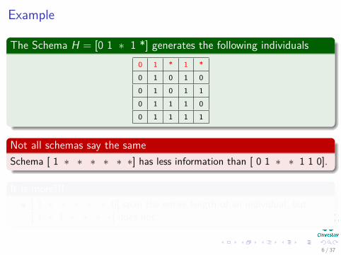
The Schema H = [0 1 ∗ 1 *] generates the following individuals0 1 * 1 *
0 1 0 1 0
0 1 0 1 1
0 1 1 1 0
0 1 1 1 1
Not all schemas say the sameSchema [ 1 ∗ ∗ ∗ ∗ ∗ ∗] has less information than [ 0 1 ∗ ∗ 1 1 0].
It is more!!![ 1 ∗ ∗ ∗ ∗ ∗ 0] span the entire length of an individual, but[ 1 ∗ 1 ∗ ∗ ∗ ∗] does not.
6 / 37
Example
The Schema H = [0 1 ∗ 1 *] generates the following individuals0 1 * 1 *
0 1 0 1 0
0 1 0 1 1
0 1 1 1 0
0 1 1 1 1
Not all schemas say the sameSchema [ 1 ∗ ∗ ∗ ∗ ∗ ∗] has less information than [ 0 1 ∗ ∗ 1 1 0].
It is more!!![ 1 ∗ ∗ ∗ ∗ ∗ 0] span the entire length of an individual, but[ 1 ∗ 1 ∗ ∗ ∗ ∗] does not.
6 / 37

Outline
1 IntroductionSchema DefinitionProperties of Schemas
2 Probability of a SchemaProbability of an individual is in schema HSurviving Under Gene wise MutationSurviving Under Single Point CrossoverThe Schema TheoremA More General VersionProblems with the Schema Theorem
7 / 37

Schema Order and Length
Definition 3 - Schema Order o (H)
Schema order, o, is the number of non “*” genes in schema H.Example: o(***11*1)=3.
Definition 3 – Schema Defining Length, δ (H).Schema Defining Length, δ(H), is the distance between first and last non“*” gene in schema H.
Example: δ(***11*1)=7-4=3.
NotesGiven an alphabet A with|A| = k, then there are (k + 1)l possibleschemas of length l .
8 / 37

Outline
1 IntroductionSchema DefinitionProperties of Schemas
2 Probability of a SchemaProbability of an individual is in schema HSurviving Under Gene wise MutationSurviving Under Single Point CrossoverThe Schema TheoremA More General VersionProblems with the Schema Theorem
9 / 37

Probabilities of belonging to a Schema H
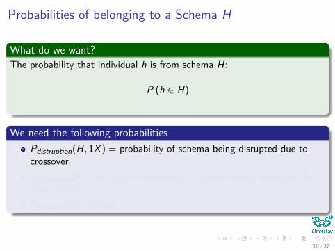
What do we want?The probability that individual h is from schema H:
P (h ∈ H)
We need the following probabilitiesPdistruption(H, 1X ) = probability of schema being disrupted due tocrossover.Pdisruption (H,mutation) =probability of schema being disrupted dueto mutationPcrossover (H survive)
10 / 37
Probabilities of belonging to a Schema H
What do we want?The probability that individual h is from schema H:
P (h ∈ H)
We need the following probabilitiesPdistruption(H, 1X ) = probability of schema being disrupted due tocrossover.Pdisruption (H,mutation) =probability of schema being disrupted dueto mutationPcrossover (H survive)
10 / 37

Probability of Disruption
Consider nowThe CGA using
I fitness proportionate parent selectionI on-point crossover (1X)I bitwise mutation with probability PmI Genotypes of length l
The Schema could be disrupted if the cross over falls between theends
Pdistruption(H, 1X ) =δ(H)
(l − 1) (1)
0 1 0 0 1 0
11 / 37

Why?
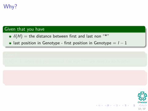
Given that you haveδ(H) = the distance between first and last non “*”last position in Genotype - first position in Genotype = l − 1
Case Iδ(H) = 1, when the positions of the non “*” are next to each other
Case IIδ(H) = l − 1, when the positions of the non “*” are in the extremes
12 / 37
Why?
Given that you haveδ(H) = the distance between first and last non “*”last position in Genotype - first position in Genotype = l − 1
Case Iδ(H) = 1, when the positions of the non “*” are next to each other
Case IIδ(H) = l − 1, when the positions of the non “*” are in the extremes
12 / 37

Why?
Given that you haveδ(H) = the distance between first and last non “*”last position in Genotype - first position in Genotype = l − 1
Case Iδ(H) = 1, when the positions of the non “*” are next to each other
Case IIδ(H) = l − 1, when the positions of the non “*” are in the extremes
12 / 37

Why?
Given that you haveδ(H) = the distance between first and last non “*”last position in Genotype - first position in Genotype = l − 1
Case Iδ(H) = 1, when the positions of the non “*” are next to each other
Case IIδ(H) = l − 1, when the positions of the non “*” are in the extremes
12 / 37
Remarks about MutationObservation about Mutation
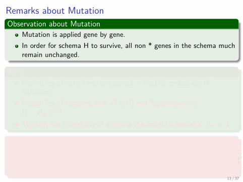
Mutation is applied gene by gene.In order for schema H to survive, all non * genes in the schema muchremain unchanged.
ThusProbability of not changing a gene 1− Pm (Pm probability ofmutation).Probability of requiring that all o(H) non * genes survive,(1− Pm)
o(H) .
Typically the probability of applying the mutation operator, pm � 1.
The probability that the mutation disrupt the schema H
Pdisruption (H,mutation) = 1− (1− Pm)o(H) ≈ o (H)Pm (2)
After ignoring high terms in the polynomial!!!13 / 37
Remarks about MutationObservation about Mutation
Mutation is applied gene by gene.In order for schema H to survive, all non * genes in the schema muchremain unchanged.
ThusProbability of not changing a gene 1− Pm (Pm probability ofmutation).Probability of requiring that all o(H) non * genes survive,(1− Pm)
o(H) .
Typically the probability of applying the mutation operator, pm � 1.
The probability that the mutation disrupt the schema H
Pdisruption (H,mutation) = 1− (1− Pm)o(H) ≈ o (H)Pm (2)
After ignoring high terms in the polynomial!!!13 / 37

Outline
1 IntroductionSchema DefinitionProperties of Schemas
2 Probability of a SchemaProbability of an individual is in schema HSurviving Under Gene wise MutationSurviving Under Single Point CrossoverThe Schema TheoremA More General VersionProblems with the Schema Theorem
14 / 37

Gene wise Mutation
Lemma 1Under gene wise mutation (Applied Gene by Gene), the (lower bound)probability of an order o(H) schema H surviving at generation (NoDisruption) t is,
1− o (H)Pm (3)
15 / 37

Probability of an individual is sampled from schema H
Consider the Following1 Probability of selection depends on
1 Number of instances of schema H in the population.2 Average fitness of schema H relative to the average fitness of all
individuals in the population.
Thus, we have the following probability
P (h ∈ H) = PUniform (h in Population)×Mean Fitness Ratio
16 / 37

Then
Finally
P (h ∈ H) =
(Number of individualsmatching schema
H at generation t)(Population Size) ×
(Mean fitness ofindividuals matching
schema H)
(Mean fitness of individuals in thepopulation)
(4)
17 / 37
Then
Finally
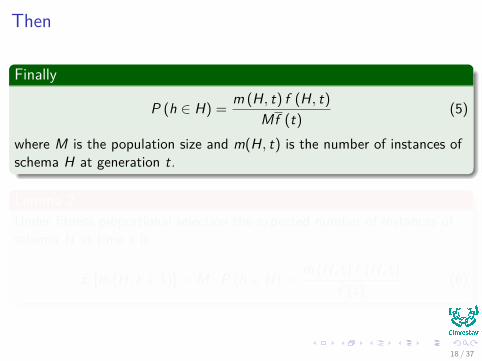
P (h ∈ H) =m (H, t) f (H, t)
Mf (t)(5)
where M is the population size and m(H, t) is the number of instances ofschema H at generation t.
Lemma 2Under fitness proportional selection the expected number of instances ofschema H at time t is
E [m (H, t + 1)] = M · P (h ∈ H) =m (H, t) f (H, t)
f (t)(6)
18 / 37

Then
Finally
P (h ∈ H) =m (H, t) f (H, t)
Mf (t)(5)
where M is the population size and m(H, t) is the number of instances ofschema H at generation t.
Lemma 2Under fitness proportional selection the expected number of instances ofschema H at time t is
E [m (H, t + 1)] = M · P (h ∈ H) =m (H, t) f (H, t)
f (t)(6)
18 / 37

Why?
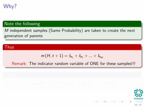
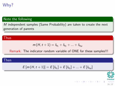
Note the followingM independent samples (Same Probability) are taken to create the nextgeneration of parents
Thus
m (H, t + 1) = Ih1 + Ih2 + ...+ IhMRemark: The indicator random variable of ONE for these samples!!!
Then
E [m (H, t + 1)] = E [Ih1 ] + E [Ih2 ] + ...+ E [IhM ]
19 / 37
Why?
Note the followingM independent samples (Same Probability) are taken to create the nextgeneration of parents
Thus
m (H, t + 1) = Ih1 + Ih2 + ...+ IhMRemark: The indicator random variable of ONE for these samples!!!
Then
E [m (H, t + 1)] = E [Ih1 ] + E [Ih2 ] + ...+ E [IhM ]
19 / 37
Why?
Note the followingM independent samples (Same Probability) are taken to create the nextgeneration of parents
Thus
m (H, t + 1) = Ih1 + Ih2 + ...+ IhMRemark: The indicator random variable of ONE for these samples!!!
Then
E [m (H, t + 1)] = E [Ih1 ] + E [Ih2 ] + ...+ E [IhM ]
19 / 37

Finally
But, M samples are taken to create the next generation of parents
E [m (H, t + 1)] = P (h1 ∈ H) + P (h2 ∈ H) + ...+ P (hM ∈ H)
Remember the Lemma 5.1 in Cormen’s Book
Finally, because P (h1 ∈ H) = P (h2 ∈ H) = ... = P (hM ∈ H)
E [m (H, t + 1)] = M × P (h ∈ H)
QED!!!
20 / 37

Finally
But, M samples are taken to create the next generation of parents
E [m (H, t + 1)] = P (h1 ∈ H) + P (h2 ∈ H) + ...+ P (hM ∈ H)
Remember the Lemma 5.1 in Cormen’s Book
Finally, because P (h1 ∈ H) = P (h2 ∈ H) = ... = P (hM ∈ H)
E [m (H, t + 1)] = M × P (h ∈ H)
QED!!!
20 / 37

Outline
1 IntroductionSchema DefinitionProperties of Schemas
2 Probability of a SchemaProbability of an individual is in schema HSurviving Under Gene wise MutationSurviving Under Single Point CrossoverThe Schema TheoremA More General VersionProblems with the Schema Theorem
21 / 37

Search Operators – Single point crossover
ObservationsCrossover was the first of two search operators introduced to modifythe distribution of schema in the population.Holland concentrated on modeling the lower bound alone.
22 / 37
Search Operators – Single point crossover
ObservationsCrossover was the first of two search operators introduced to modifythe distribution of schema in the population.Holland concentrated on modeling the lower bound alone.
22 / 37

CrossoverConsider the following
Generated Individual h = 1 0 1 | 1 1 0 0H1 = * 0 1 | * * * 0H2 = * 0 1 | * * * *
Crossover
Remarks1 Schema H1 will naturally be broken by the location of the crossover
operator unless the second parent is able to ‘repair’ the disruptedgene.
2 Schema H2 emerges unaffected and is therefore independent of thesecond parent.
3 Thus, Schema with long defining length are more likely to bedisrupted by single point crossover than schema using shortdefining lengths.
23 / 37
Now, we have
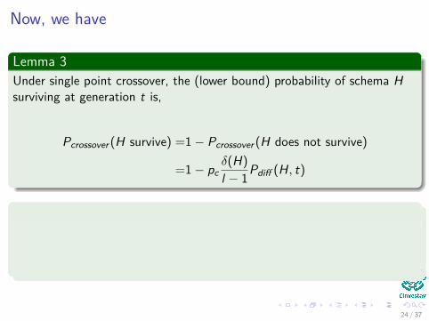
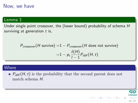
Lemma 3Under single point crossover, the (lower bound) probability of schema Hsurviving at generation t is,
Pcrossover (H survive) =1− Pcrossover (H does not survive)
=1− pcδ(H)
l − 1Pdiff (H, t)
WherePdiff (H, t) is the probability that the second parent does notmatch schema H.pc is the a priori selected threshold of applying crossover.
24 / 37
Now, we have
Lemma 3Under single point crossover, the (lower bound) probability of schema Hsurviving at generation t is,
Pcrossover (H survive) =1− Pcrossover (H does not survive)
=1− pcδ(H)
l − 1Pdiff (H, t)
WherePdiff (H, t) is the probability that the second parent does notmatch schema H.pc is the a priori selected threshold of applying crossover.
24 / 37
How?
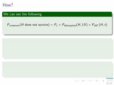
We can see the following
Pcrossover (H does not survive) = Pc × Pdistruption(H, 1X )× Pdiff (H, t)
After allPc is used to decide if the crossover will happen.The second parent could come from the same schema, and yes!!! Wedo not have a disruption!!!
Then
Pcrossover (H does not survive) = Pc ×δ(H)
l − 1 × Pdiff (H, t)
25 / 37

How?
We can see the following
Pcrossover (H does not survive) = Pc × Pdistruption(H, 1X )× Pdiff (H, t)
After allPc is used to decide if the crossover will happen.The second parent could come from the same schema, and yes!!! Wedo not have a disruption!!!
Then
Pcrossover (H does not survive) = Pc ×δ(H)
l − 1 × Pdiff (H, t)
25 / 37

In addition
Worst case lower bound
Pdiff (H , t) = 1 (7)
26 / 37

Outline
1 IntroductionSchema DefinitionProperties of Schemas
2 Probability of a SchemaProbability of an individual is in schema HSurviving Under Gene wise MutationSurviving Under Single Point CrossoverThe Schema TheoremA More General VersionProblems with the Schema Theorem
27 / 37
The Schema Theorem
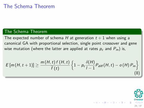
The Schema TheoremThe expected number of schema H at generation t + 1 when using acanonical GA with proportional selection, single point crossover and genewise mutation (where the latter are applied at rates pc and Pm) is,
E [m (H, t + 1)] ≥ m (H, t) f (H, t)f (t)
{1− pc
δ(H)
l − 1Pdiff (H, t)− o (H)Pm
}(8)
28 / 37

Proof
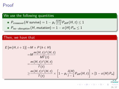
We use the following quantitiesPcrossover (H survive) = 1− pc δ(H)
l−1 Pdiff (H, t) ≤ 1Pno−disruption (H,mutation) = 1− o (H)Pm ≤ 1
Then, we have that
E [m (H, t + 1)] =M × P (h ∈ H)
=Mm (H, t) f (H, t)Mf (t)
=m (H, t) f (H, t)
f (t)
≥m (H, t) f (H, t)f (t)
×[1− pc
δ(H)
l − 1Pdiff (H, t)]× [1− o (H)Pm]
29 / 37

Proof
We use the following quantitiesPcrossover (H survive) = 1− pc δ(H)
l−1 Pdiff (H, t) ≤ 1Pno−disruption (H,mutation) = 1− o (H)Pm ≤ 1
Then, we have that
E [m (H, t + 1)] =M × P (h ∈ H)
=Mm (H, t) f (H, t)Mf (t)
=m (H, t) f (H, t)
f (t)
≥m (H, t) f (H, t)f (t)
×[1− pc
δ(H)
l − 1Pdiff (H, t)]× [1− o (H)Pm]
29 / 37

Thus
We have the following
E [m (H, t + 1)] ≥m (H, t) f (H, t)f (t)
[1− pc
δ(H)
l − 1Pdiff (H, t)− o (H)Pm + ...
pcδ(H)
l − 1Pdiff (H, t)o (H)Pm
]≥m (H, t) f (H, t)
f (t)
[1− pc
δ(H)
l − 1Pdiff (H, t)− o (H)Pm
]
The las inequality is possible because pc δ(H)l−1 Pdiff (H, t)o (H)Pm ≥ 0
30 / 37

Remarks
ObservationsThe theorem is described in terms of expectation, thus strictlyspeaking is only true for the case of a population with an infinitenumber of members.
I What about a finite population?I In the case of finite population sizes the significance of population drift
plays an increasingly important role.
31 / 37

Outline
1 IntroductionSchema DefinitionProperties of Schemas
2 Probability of a SchemaProbability of an individual is in schema HSurviving Under Gene wise MutationSurviving Under Single Point CrossoverThe Schema TheoremA More General VersionProblems with the Schema Theorem
32 / 37

More General Version
More General Version
E [m (H, t + 1)] ≥ m (H, t)α (H, t) {1− β(H, t)} (9)
Whereα(H, t)is the “selection coefficient”β(H, t) is the “transcription error.”
This allows to say that H survives if
α(H, t) ≥ 1− β (H, t) orm (H, t) f (H, t)
f (t)≥
{1− pc
δ(H)
l − 1Pdiff (H, t)− o (H)Pm
}
33 / 37
More General Version
More General Version
E [m (H, t + 1)] ≥ m (H, t)α (H, t) {1− β(H, t)} (9)
Whereα(H, t)is the “selection coefficient”β(H, t) is the “transcription error.”
This allows to say that H survives if
α(H, t) ≥ 1− β (H, t) orm (H, t) f (H, t)
f (t)≥
{1− pc
δ(H)
l − 1Pdiff (H, t)− o (H)Pm
}
33 / 37

More General Version
More General Version
E [m (H, t + 1)] ≥ m (H, t)α (H, t) {1− β(H, t)} (9)
Whereα(H, t)is the “selection coefficient”β(H, t) is the “transcription error.”
This allows to say that H survives if
α(H, t) ≥ 1− β (H, t) orm (H, t) f (H, t)
f (t)≥
{1− pc
δ(H)
l − 1Pdiff (H, t)− o (H)Pm
}
33 / 37

Observation
ObservationThis is the basis for the observation that short (defining length), low orderschema of above average population fitness will be favored by canonicalGAs, or the Building Block Hypothesis.
34 / 37

Outline
1 IntroductionSchema DefinitionProperties of Schemas
2 Probability of a SchemaProbability of an individual is in schema HSurviving Under Gene wise MutationSurviving Under Single Point CrossoverThe Schema TheoremA More General VersionProblems with the Schema Theorem
35 / 37

Problems
Problem 1Only the worst-case scenario is considered.No positive effects of the search operators are considered.This has lead to the development of Exact Schema Theorems.
Problem 2The theorem concentrates on the number of schema surviving notwhich schema survive.Such considerations have been addressed by the utilization of Markovchains to provide models of behavior associated with specificindividuals in the population.
36 / 37
ProblemsProblem 3
Claims of “exponential increases” in fit schema i.e., if the expectationoperator of Schema Theorem is ignored and the effects of crossoverand mutation discounted, the following result was popularized byGoldberg,
m(H, t + 1)≥(1+ c)m(H, t)
where c is the constant by which fit schema are always fitter than thepopulation average.
PROBLEM!!!Unfortunately, this is rather misleading as the average populationfitness will tend to increase with t,
I thus population and fitness of remaining schema will tend to convergewith increasing ‘time’.
37 / 37