08 decrease and conquer spring 15

Instructor:Sadia Arshid, DCS& SE 1

Decrease and Conquer


Decrease-and-conquer algorithm works as follows:◦ Establish the relationship between a solution to a

given instance of a problem and a solution to a smaller instance of the same problem.

◦ Exploit this relationship either top down (recursively) or bottom up (without a recursion).

Basics


Decrease by a constant◦ The size of an instance is reduced by the same

constant (usually one) at each iteration of the algorithm.

Decrease by a constant factor◦ The size of a problem instance is reduced by the

same constant factor◦ (usually two) on each iteration of the algorithm.

Variable size decrease◦ A size reduction pattern varies from one iteration

to another

Decrease & Conquer variations


Decrease by Constant


Insertion sort is based on the decrease (by one)-and-conquer approach:◦ Provided that a smaller array A[1..n - 1] is

already sorted.◦ Find an appropriate position for an element A[n ]◦ among the sorted n - 1 elements and insert it

there. Right-to-left scan:

◦ Scan the sorted subarray from right to left until the firstelement smaller than or equal to A[n ] is encounteredand then insert A[n ] right after that element.

Insertion Sort


Algorithm InsertionSort (A[1..n ])for i ← 2 to n do

v ← A[i]j ← i - 1while j > 0 and A[j] > v do

A[j + 1] ← A[j]j ← j - 1

A[j + 1] ← v


Input size: n Basic operation: key comparison A[j] > v. The worst case occurs when the input is

already an array of strictly decreasing values:W(n)=∑ ∑ 1 = n(n-1)/2=є Ө (n 2 )

Best Case: B(n)=∑ 1=n-1єӨ(n)

Efficiency

n

i=2j=1

i-1

n

i=2


for given i there can be i slots where x can be inserted, and each slot is equally probable of holding this value, thus each slot has probability 1/i,

following are number of comparison for each slot

Average Case

slot number of Comparison

i 1

i-1 2

i-2 3

. .

. .

. .

2 i-1

1 i-1


average number of comparisons needed to insert x is1(1/i)+2(1/i)+………..(i-1)(1/i)+(i-1)(1/i)=1/i(1+2+…..i-1)+(i-1)(1/i)=1/i(i(i-1)/2)+(i-1)(1/i)=(i+1)/2-1/i……………………(eq1)these are number of comparisons require in each

for loop iterationA(n)=∑ (i+1)/2 -1/i

=1/2∑ (i+1) - ∑ 1/i

A(n)=(n+4)(n-1)/4-lgn≈n 2 /4єӨ(n 2 )

n

i=2

n

i=2

n

i=2


When given a graph, we are often interested in searching the vertices in the graph in some organized way.◦ Depth-first search (DFS) starts visiting a graph at

some arbitrary unvisited vertex.◦ When a vertex is visited, a flag is marked to indicate

that it has been visited.◦ At each vertex v, DFS recursively visits an unvisited

neighbour of v.◦ If there are no unvisited neighbour, recursion step

and backs up. It is convinenit to use stack in DFS

◦ push vertex on the stack when visited first time◦ pop it when all of it becomes dead end

Depth First Search


set DFSnumber for all vertices to be -1count = 0for each unvisited vertex v (DFSnumber == -1)

dfs(v, count)---dfs(v, int &count){

set DFSnumber[v] = count++for each w adjacent to v

if DFSnumber[w] == -1dfs(w, count)

}

DFS


Stack Ordering:a16c25 f44d31 b53 e62

b

ea

d

c f

a

e

b

f

d

c


Every vertex is traversed once.◦ For each vertex, we need to process all its neighbours.◦ Adjacency matrix: (n^2) operations

Yields two distinct ordering of vertices:◦ preorder: as vertices are first encountered (pushed

onto stack)◦ postorder: as vertices become dead-ends (popped off

stack)

Applications:◦ checking connectivity, finding connected components◦ checking acyclicity◦ searching state-space of problems for solution (AI)

DFS


Explore graph moving across to all the neighbors of last visited vertex

Similar to level-by-level tree traversals Instead of a stack, breadth-first uses queue Applications: same as DFS, but can also

find paths from a vertex to all other vertices with the smallest number of edges

Breadth First Search


BFS(G)count :=0mark each vertex with 0for each vertex v∈ V do

bfs(v)----------------------------

bfs(v)count := count + 1mark v with countinitialize queue with vwhile queue is not empty do

a := front of queuefor each vertex w adjacent to a do

if w is marked with 0count := count + 1mark w with countadd w to the end of the queue

remove a from the front of the queue

BFS


b

ea

d

c f

a

dc e

f

b


Every vertex is traversed once.◦ For each vertex, we need to process all its

neighbours.◦ Adjacency matrix: (n^2) operations

Yields single ordering of vertices (order added/deleted from queue is the same)

Applications◦ Checking connectivity.◦ Cycle detection.◦ Shortest path (unweighted graph).

Effieceincy


Data structures: stack vs. queue Implementation: recursion vs. explicit

queue manipulation Complexity: same

DFS vs BFS


Decrease By constant Factor

BINARY SEARCH

Function location(low,high) if low<=high

mid=floor((low+high)/2)if x=s[mid]

return midelse if x<s[mid] location=location(low,mid-1)

else location=location(mid+1,high)

20Instructor: Sadia Arshid, DCS

&SE

Binary Search –Complexity Analysis Case Complexity : Worst case w(n)=floor(w(n/2))+1

◦ searching an array sized N requires one examination of the element in the middle, followed by a binary search of either the left half or the right half of the array, each of which has N/2 elements.

terminating condition/initial condition : w(1)=1


&SE

w(n)=w( n/2)+1 w(n/2)=w(n/4)+1 w(n/4)=w(n/8)+1by backward substitutionw(n)=w(n/4)+2=w(n/8)+3=w(n/ 2k )+kby taking 2k =nw(n)=w(1)+k=k=lg(n)+1 є O(lgn)


&SE


The fake coin problem is to detect a single fake coin from a set of coins using a balance scale.

Supposing the fake coin is lighter, we can repeatedly compare one half of a set to the other half, eliminating the heavier half.

This decreases the number of coins in half each iteration, so only ≈ log2 n weighings are needed.

The Fake Coin Problem


To multiply two pos. integers n · m by this method:

m if n = 1 n.m = (n/2) · 2m if n is even (⌊n/2⌋ · 2m + m if n is odd

Russian Peasant multiplication


n m

50 65

25 130

12 260 +130

6 520

3 1040

1 2080 +1040

2080+(130+1040)

3250


Decrease By variable size


Interpolation search (sometimes referred to as extrapolation search) is an algorithm for searching for a given key value in an indexed array that has been ordered by the values of the key.◦ checking telephone index◦ finding some word dictionary

Interpolation Search


work for uniformly distributed data calculation of mid is modified as mid

=low+(((x-s[low])(high-low))/s(high)-s(low))

Average case: lg(lg(n)) worst Case: O(n)

Interpolation Search (Contd…)


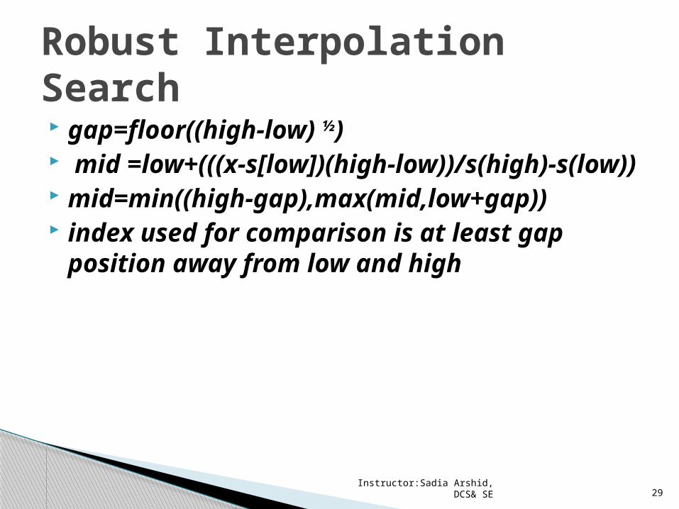
gap=floor((high-low) ½) mid

=low+(((x-s[low])(high-low))/s(high)-s(low))

mid=min((high-gap),max(mid,low+gap))

index used for comparison is at least gap position away from low and high

Robust Interpolation Search


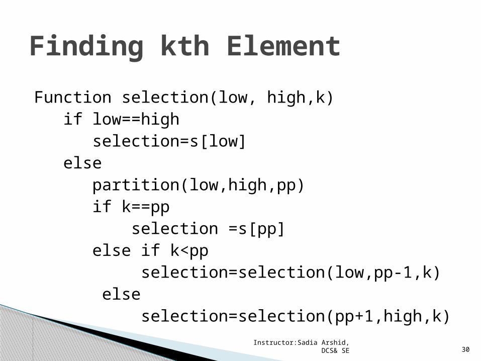
Function selection(low, high,k) if low==high selection=s[low] else partition(low,high,pp) if k==pp selection =s[pp] else if k<pp selection=selection(low,pp-1,k) else selection=selection(pp+1,high,k)

Finding kth Element


procedure partition(low,high,pivotpoint)pivotitem=s[low], j=lowfor i=low+1 to high

if s[i]<pivotitmj=j+1exchange s[i] & s[j]

pivotpoint=jexchange s[low] & s[pivotpoint]


w(n)=w(n-1)+n-1 =w(n-2)+n-2+n-1 =w(n-3)+n-3+n-2+n-1 ….. =1+2+3+…..+n-1 =n(n-1)/2єӨ(n2 ) Best Case B(n)= n-1 єӨ(n )

Worst case


We assume that all inputs are equal likely to be pivot point ie pp=k

Average Case

Input size in recursive call Number of outcomes yield that input size

0 n

1 pp=2, pp=n-1 and k=1 or k=n 2

2, pp=3, pp=n-2 and k=1,2 or n-1, n 4

3 6

i 2(i)

n-1 2(n-1)


A[n]=(sum of (number of outcomes yield that input size)(input size of recursive call)/sum of numbers )+complexity of partition

=(nA(0)+2(A(1)+4A(2)+6A(3)……+2n-1(An-1)/n+2(1+2+3+…+n-1))+n-1

A(0)=0= 2(A(1)+2A(2)+3A(3)……+n-1(An-1))/n+2(n(n-1)/2) ))+n-1=2(A(1)+2A(2)+3(A(3)……+n-1(An-1))/n2 ) +n-1n2A(n)= 2(A(1)+2A(2)+3(A(3)……+n-1(An-1))+n2( n-1)

……………….eq(1)replacing n with n-1(n-1)2A(n-1)= 2(A(1)+2A(2)+3(A(3)……+n-2(An-2))+(n-1)2( n-2)

……………….eq(2)subtracting eq2 from eq1A(n)= (n2-1)A(n-1)/n2+(n-1)(3n-2)/n2

for larger n A(n)≈A(n-1)+3 ≈A(n-2)+3+3 ≈A(n-i)+3iby taking A(0)=0, i=n ≈3nєӨ(n)


Euclid’s s algorithm gcd(m,n)= gcd( n, m mod n) size, number, measured by the second

number iterations are based on repeated application

of equality gcd( m, n) Example: gcd(80,44) = gcd(44,36) =

gcd(36, 8) = gcd(8,4) = gcd(4,0) 4 One can prove that the size decreases at least by half after two consecutive iterations

Euclid’s Algorithm


m>n, input size is reduced by m mod n in each

iteration, there could be two cases Case 1:

◦ if n<m/2, (m mod n) < (n) <=m/2 Case2:

◦ if n>m/2, (m mod n)= (m-n) < m/2◦ size is almost reduced by half◦ so T(n)єӨ(lg n)

08 decrease and conquer spring 15

Software