1 a multiple-detection probability hypothesis density...
TRANSCRIPT

1
A Multiple-Detection Probability Hypothesis
Density Filter
Xu Tanga,b Xin Chenb Mike McDonaldc Ronald Mahlerd and T. Kirubarajanb
aDepartment of Electronic Engineering, University of Electronic Science and Technology of China,
Chengdu, Sichuan, R.P.China
bDepartment of Electrical and Computer Engineering, McMaster University, Hamilton, Ontario, Canada
cDefence R&D Canada, Ottawa, Canada
dLockheed Martin Advanced Technology Laboratories, U.S.A.
Abstract
Most conventional target tracking algorithms assume that one target can generate at most one detection per scan.
However, in many practical target tracking applications, one target may generate multiple detections in one scan,
because of multipath propagation, or high sensor resolution or some other reason. If the multiple detections from the
same target can be effectively utilized, the performance of the multitarget tracking system can be improved. However,
the challenge is that the uncertainty in the number of target and the many-to-one measurement set-to-target association
will increase the complexity of tracking algorithms. To solve this problem, the random finite set (RFS) modeling
and the random finite set statistics (FISST) are used in this paper. Without any extra approximation beyond those
made in the standard probability hypothesis density (PHD) filter, a general multi-detection PHD (MD-PHD) update
formulation is derived. It is also established in this paper that, with certain reasonable assumptions, the proposed
MD-PHD recursion can function as a generalized extended target PHD or multisensor PHD filter. Furthermore, a
Gaussian Mixture (GM) implementation of the proposed MD-PHD formulation, called the MD-GM-PHD filter, is
presented. The proposed MD-GM-PHD filter is demonstrated on a simulated over-the-horizon radar (OTHR) scenario.
Index Terms
Target tracking, Bayesian filtering, Random finite sets, Probability hypothesis density filter, Multiple-detection
tracking, Gaussian mixture, Over-the-horizon radar (OTHR).
I. INTRODUCTION
In many multitarget tracking algorithms, such as the Multiple Hypothesis Tracker (MHT) [1], [2], the Joint
Probabilistic Data Association Filter (JPDAF) [3]–[6], and algorithms based on the random finite set (RFS) method
[7], [8], a common assumption is that in every scan there is at most one measurement from one target. But in many
practical scenarios, one target may generate multiple detections in a single frame via different signal propagation
paths, (i.e., via different measurement modes [9]). Some common examples include multitarget tracking systems
March 7, 2014 DRAFT
DRDC-RDDC-2014-P136

2
using the over-the-horizon radar (OTHR) [10], where radar signals from the same target are scattered by different
ionospheric layers, and the passive coherent location (PCL) system with multistatic configuration [11], where one
target can generate multiple detections from different transmitters of opportunity [12]. In such situations, if the
tracking algorithm is able to properly extract the information in the multiple detections, the estimation accuracy
can be improved and the number of false tracks can be reduced. However, the complexity of the tracking algorithm
increases significantly due to the additional measurement mode uncertainty [9]. In the literature, various techniques
have been proposed to address the multiple-detection problem in OTHR [13]–[20] or PCL [12], [21] scenarios.
Recently, two multitarget tracking algorithms that are able to deal with the multi-detection problem were proposed.
One is the Multiple Detection Multiple Hypothesis Tracker (MD-MHT) [22], which uses the MHT framework. The
other is the Multiple-Detection Joint Probabilistic Data Association Filter (MD-JPDAF) [9], which uses the JPDA
framework. Both of them can exploit the available measurement mode information to effectively track multiple
targets.
In multitarget tracking, it is possible to model the set of target states and the set of observations as two RFSs and
handle them using the RFS Bayesian filtering framework. One tractable Bayesian solution under the RFS framework
is the probability hypotheses density (PHD) filter [7], [23]. The PHD filter is a recursion that propagates the first
order statistical moment, or the intensity of the RFS of states over time [7]. It can track multiple target states and
keep track of the number of targets without explicit multitarget data association between measurements and tracks.
Note that the standard PHD filters [24] rely on the assumption of a single detection per target.
In [25], the multiple-detection single-target tracking problem was addressed under the RFS framework. The
target-generated measurements are modeled as a mixture of one binary RFS and one Poisson RFS, which represent
the single direct path measurement and other multipath measurements, respectively. Consequently, it cannot handle
a general situation where the preferred (direct) path is absent, e.g., tracking using the OTHR. Moreover, there is
no distinction among the various modes of detection, which will result in loss of information or in spurious tracks.
In this paper, we address the multitarget tracking problem with multiple detections within the RFS theoretical
framework. A novel PHD measurement-update equation that accommodates multiple detections is derived using the
finite-set statistics (FISST) theory [23]. No approximation beyond those in the standard PHD formula is made in
the derivation of the new multiple detection PHD (MD-PHD) filter.
The MD-PHD filter proposed here has a more general application as well. The MD-PHD equations derived under
the multiple detection assumptions can deal with multitarget tracking with multipath propagation effects, extended
targets, multiple sensors, or multiple detections with multiple sensors, respectively. We also show that the proposed
MD-PHD filter can be transformed into the extended target PHD [26] or reduced to the generalized multisensor
PHD in [27], [28].
Furthermore, a closed form implementation of the MD-PHD filter is presented using the Gaussian Mixture (GM)
representation, called the multi-detection GM-PHD (MD-GM-PHD) filter. The proposed MD-GM-PHD algorithm
is demonstrated on a simulated OTHR multitarget tracking scenario. The performance of the MD-GM-PHDF is
compared with the latest association based technique, MD-JPDAF [9], for a fixed number of targets, and with the
March 7, 2014 DRAFT

3
conventional GM-PHDF for a dynamic number of targets. Results show the effectiveness of the new algorithm with
respect to estimation accuracy and ability to handle a time-varying number of targets.
The rest of the paper is organized as follows. A brief introduction of multitarget tracking with multiple detections
and the conventional PHD filter is given in Section II. The MD-PHD is described in Section III. Section IV presents
the generalization of the proposed MD-PHD and the connection to other PHD formulations. The GM implementation
of the proposed MD-PHD is presented in Section V. Simulation results can be found in Section VI. Conclusions
are in Section VII.
II. BACKGROUND AND PRELIMINARIES
In this section, we first describe the problem of multiple-detection multitarget tracking. Then we present the
mathematical preliminaries on the RFS and the PHD filter.
A. Multiple-Detection Multitarget Tracking
In the multi-target tracking problem, the evolution of the objects’ states and the origin of measurements are
unknown. Uncertainty in target state and sensor measurement can be modelled by an RFS. Assume that there
are Nx,k targets with states x1k, ...,x
Nx,k
k , each taking values in a state space X ⊆ Rnx , and Nz,k measurements
z1k, ..., zNz,k
k , each taking values in an observation space Z ⊆ Rnz . The multi-target state and the multi-target
observation are then represented by the RFS: Xk = {x1k, ...,x
Nx,k
k } and Zk = {z1k, ..., zNz,k
k }, respectively. Here,
nx and nz are the dimension of the target state vector and the measurement vector, respectively.
The dynamic evolution of each target state xik in the RFS Xk is modeled by the state equation
xik+1 = fk(x
ik) + vk (1)
where fk is a known linear or non-linear state transition function, vk is a zero-mean white Gaussian process noise
sequence with covariance matrix Qk that models targets maneuver. Each target evolves independently.
For the multiple-detection system, we assume that there are L possible measurement modes with known mea-
surement equations, and zjk, the jth measurement at time k, is given by
zjk =
⎧⎪⎪⎪⎪⎪⎪⎪⎪⎪⎪⎪⎪⎪⎨⎪⎪⎪⎪⎪⎪⎪⎪⎪⎪⎪⎪⎪⎩
h1k(xi) +w1
k if mode 1
h2k(xi) +w2
k if mode 2
...
hLk (xi) +wL
k if mode L
zjk if clutter
(2)
where hlk(·), l = 1, 2, ...L is the measurement function associated with the l-th measurement mode and wl
k is the
corresponding measurement noise, which is assumed to be zero-mean Gaussian random variable with covariance
matrix Rlk and is independent of the target state. Associations between target xi
k, measurement zjk, and mode l
March 7, 2014 DRAFT

4
are unknown to the tracker. The false measurement zk is assumed to be uniformly distributed in the surveillance
volume of the sensors and the number of false alarms per scan is Poisson distributed with mean λ.
Remark: In practice, the multiple detections for a given target might be generated with unknown modes, or with
a time-varying number of mode. For simplicity, we assume that the number of modes L is constant and the mode
information is known. The same assumptions are made in [9] and [22].
The objective of this paper is to estimate the RFS Xk given the measurement RFS Zk from the sensor. We
achieve this within the framework of the recursive multitarget Bayesian PHD filter [23].
B. Background to the PHD filter
For RFS Ξ, one can define the probability density function fΞ(X) on the finite set variable X , and fΞ(X)
satisfies the unit requirement
f(∅) +∞∑
n=1
1
n!
∫fΞ({x1, . . . ,xn})dx1 . . . dxn = 1 (3)
where n! counts the duplication caused by the permutation of {x1,x2, . . . ,xn}, and f(∅) denotes the probability
of the empty set.
Based on the RFS theory, the multitarget Bayes filter can be derived. However, the multitarget Bayes filter is
computationally intractable in all but the simplest scenarios since the calculation of the multitarget Bayes filter
relies on the set integral, which needs to take into account all possible multitarget state finite sets [23]. To conquer
this problem, the first-order multitarget statistical moment, or the PHD, has been used [24]. For a given RFS Ξ
with the multitarget probability density function fΞ(X), the PHD DΞ(x) can be calculated by
DΞ(x) =
∫δX(x)fΞ(X)δX (4)
where δX(x) �∑
w∈X δ(x − w) and δ(x) is the Dirac delta function, which is used to convert the finite set
X = {x1,x2, . . . ,xn} into vectors since the first-order statistical moment is defined in the vector space.
Then, by approximating the predicted multitarget state as a Poisson point process, the PHD filter is developed
in [24], where the PHD is propagated in a recursive form:
• Prediction equation:
Dk+1|k(x) = bk+1(x) +
∫Fk+1|k(x|x′)Dk|k(x′)dx′ (5)
where
Fk+1|k(x|x′) � pS(x′)fk+1|k(x|x′) (6)
and fk+1|k(x|x′) is the Markov transition density for the single target state; pS(x′) is the surviving probability
for the existing targets; bk+1(x) is the PHD for the newborn targets that appear at scan k+1. Note that it has
been assumed for simplicity that no targets are spawned from the existing ones.
• Measurement update equation:
Dk+1|k+1(x) ∼= LZk+1(x)Dk+1|k(x) (7)
March 7, 2014 DRAFT

5
where the pseudo-likelihood function is given by
LZk+1(x) � qD(x) +
∑z∈Zk
pD(x)hk+1(z|x)λk+1(z) + τk+1(z)
(8)
and hk+1(z|x) denotes the sensor likelihood function; pD(x) is the abbreviation of pD,k+1(x) and represents the
target detection probability at scan k+1 for the target with state x; qD(x) = 1−pD(x); λk+1(zk+1) represents the
intensity function of clutter points; τk+1(z) =∫pD(x)fk+1(z|x)Dk+1|k(x)dx is the intensity of the measurement
z ∈ Zk.
Note that above “classical” PHD filter makes the following simplifying assumptions [28]: (1) there is only a
single sensor; (2) all target motions are independent; (3) measurements are conditionally independent of the target
states; (4) the clutter process is Poisson; and (5) target-generated measurements are Bernoulli.
III. MULTI-DETECTION PHD FILTER
In this section we derive the formula for the proposed MD-PHD recursion. The difference between the MD-PHD
and the conventional single-detection PHD filter is in the measurement update equation (i.e., the corrector step).
Thus, only the measurement update equation of the MD-PHD filter will be presented.
A. Multi-detection Measurement Model
To derive the MD-PHD, the following assumptions are made.
Assumption 1: There are L measurement modes, each with a known measurement likelihood function:
f lk+1(z|x) = fwl
k+1(z− hl
k+1(x)), l = 1, ..., L (9)
where fwlk+1
(·) is the probability density function of the measurement noise wlk+1.
Assumption 2: There is at most one detection generated by a target through a specific mode.
Assumption 3: The detection probability, denoted in plD, of each mode l can be different.
Based on the above assumptions, we develop the likelihood function of multi-detection measurements for one
target as follows by using the FISST formulas of [23]. The detailed derivation is given in the Appendix.
For single target state x and its corresponding measurement set W , if W = ∅, one has the probability that the
target with state x is undetected in all modes as
fk+1(W |x) = fk+1(∅|x) =L∏
l=1
(1− plD(x)
)(10)
Suppose W = {z1, ..., zm} with |W | = m ≤ L, then one has
fk+1(W |x) =L∏
l=1
(1− plD(x)
)∑θ
∏θ(l)>0
plD(x) · hlk+1(zθ(l)|x)
1− plD(x)(11)
where hlk+1
(z|x) is the sensor measurement likelihood function with mode l, and the summation is taken over all
association hypotheses θ : {1, ..., L} → {0, 1, ...,m}, which is defined in Section 10.5.4 of [23]. For instance, with
March 7, 2014 DRAFT

6
L = 3 and W = {z1, z2} (i.e., m = 2), the corresponding likelihood function is
fk+1(W |x) = (1− p1D(x)) · p2D(x) · p3D(x) · f2k+1
(z1|x) · f3k+1(z2|x)
+ (1− p1D(x)) · p3D(x) · p2D(x) · f3k+1(z1|x) · f2
k+1(z2|x)
+ (1− p2D(x)) · p3D(x) · p1D(x) · f3k+1(z1|x) · f1
k+1(z2|x)
+ (1− p2D(x)) · p1D(x) · p3D(x) · f1k+1(z1|x) · f3
k+1(z2|x)
+ (1− p3D(x)) · p2D(x) · p1D(x) · f1k+1(z1|x) · f2
k+1(z2|x)
+ (1− p3D(x)) · p1D(x) · p2D(x) · f2k+1(z1|x) · f1
k+1(z2|x)
(12)
B. MD-PHD Measurement-update Equation
In the MD-PHD measurement-update step, one has to consider the possibility that multiple elements in the current
measurement set Zk+1 might have originated from the same target. This special form of PHD measurement-update
equation involves combinatorial sums taken over all partitions of Zk+1, and its derivation is cumbersome [28].
Fortunately, the general chain rule (GCR) to simplify the derivation progress was introduced in [28]. A general
PHD measurement-update expression with the following pseudo-likelihood function was provided:
LZk+1(x) = (1− pD(x)) +
∑P∠Zk+1
ωP∑W∈P
LW (x)
κW + τW(13)
where
LW (x) = fk+1(W |x) (14)
1− pD(x) = L∅(x) = fk+1(∅|x) (15)
and
κW =δ log κk+1
δW[0] (16)
where κk+1[g] is the probability generating functional (p.g.fl.) of the clutter process, which is assumed to be a
Poisson point process. As a result, κW is given by
κW =
⎧⎪⎪⎪⎪⎪⎨⎪⎪⎪⎪⎪⎩
−λk+1 if W = ∅
κk+1(z) if W = {z}
0 if |W | > 1
(17)
In (13), the summation is taken over all partitions P of the current measurement RFS Zk+1, the notation “P∠Zk+1”
stands for “P partitions Zk+1 into cell W ”, and
τW =
∫LW (x) ·Dk+1|k(x)dx (18)
ωP =
∏W∈P
(κW + τW )∑P′∠Zk+1
∏W ′∈P′
(κW ′ + τW ′)(19)
March 7, 2014 DRAFT

7
Note that (13) is a concise symbolic equation, which does not characterize any specific form for the probability
of detection pD(x) or the target likelihood function LW (x). This makes it possible to advance the PHD with more
general target measurement-generation models [28], e.g., the second-generation PHDs [29]. Our work also benefits
from it.
Substituting (10) and (11) into (13), one gets the MD-PHD pseudo-likelihood function as
LZk+1(x) = (1− pD(x)) +
∑P∠Zk+1
ωP∑W∈P
LW (x)
κW + τW
=
(L∏
l=1
(1− plD(x)
))+
∑P∠Zk+1
ωP∑W∈P
L∏l=1
(1− plD(x)
)∑θ
∏θ(l)>0
plD(x)·hl
k+1(zθ(l)|x)1−pl
D(x)
κW + τW
(20)
Note that distinct partition methods are needed for different second-generation PHDs, e.g. the extended target
PHD [26] or the multisensor PHD [27]. Aside from the partition defined in [26] and [27], we define a Lmax-
partition. It restricts that for each W ∈ P , the total number of elements in W is no larger than L. For example, let
Zk+1 = {z1, z2, z3} with |Zk+1| = 3 and L = 2. Then, the Lmax-partitions of Zk+1 are
P1 = {{z1}, {z2}, {z3}} ,where W1 = {z1},W2 = {z2},W3 = {z3}
P2 = {{z1, z2}, {z3}} ,where W1 = {z1, z2},W2 = {z3}
P3 = {{z1, z3}, {z2}} ,P4 = {{z2, z3}, {z1}} ,P5 = {{z1, z2, z3}}The summation in (20) is taken over all such Lmax-partitions, P , of the current measurement RFS Zk+1.
Note the following test for consistency: If the mode number L is reduced to 1, the MD-likelihood function (11)
will reduce to the normal single-target likelihood function fk+1(z|x) with a single-detection. In addition, there will
be only a singleton in the partition of the RFS Zk+1. Thus, the MD-PHD pseudo-likelihood function (20) will
reduce to the conventional single-detection PHD pseudo-likelihood function (8).
IV. GENERALIZING THE MD-PHD FILTER
The multi-detection is a general concept and can characterize broader physical measurement models. Thus, in
this section, the MD-PHD is used to handle various multi-detection applications under different assumptions and
measurement models.
A. A General Multipath-aided PHD Filter
The MD-PHD proposed in Section III can be used for target tracking with multipath measurements. In a scenario
with multipath measurements, there are many signal propagation paths between a target and the receiver. Among
them, L resolved paths, e.g., those scattered from the target and reflected at most once from a reflection point, are
considered. We assume that one knows the geometry of the surface, reflection points, and the reflection coefficients.
However, the target detection probability can be path-dependent. A common example of this model is the OTHR
[9] [10]. Thus, we can cast the measurement mode defined in (2) to each multiple propagation path. Consequently,
March 7, 2014 DRAFT

8
the uncertain association of the multipath reflection, which arises from the exploitation of the information in all
paths by the algorithm, can be handled by the likelihood function (11) in the MD-PHD recursion.
B. A General Extended Target PHD Filter
In target tracking with a high resolution radar, the extended nature of a target also generates multiple detections
at each scan. More specifically, we assume that there are l = 0, ..., L number of detections from a collection of
reflection points, whose number is bigger than L, on the surface of the extended target. Each detection is related to
a deterministic measurement model with different observability from the receiver. Then the detected measurements
can be modeled by the measurement mode in (2) with a different detection probability for each mode.
In this sense, the multi-detection likelihood function (11) becomes a general extended target likelihood function
and it has the same expression as the single extended target likelihood function (12.215) in [23], As a result, the
proposed MD-PHD filter, defined by (11), (20) and the Lmax-partitions in Section III-B, can be an extended target
PHD filter.
Compared with the existing extended target PHD filter in [26], our MD-PHD filter relaxes the Poisson approx-
imation for the target-originated measurements in [26]. Thus, it can deal with more general issues in multiple
extended targets tracking, e.g., in high-resolution sensor observation scenarios where detailed measurement modes
for individual reflection points on the target are known.
C. A General Multisensor PHD Filter
Under the multisensor PHD filter framework [27], the measurements from each sensor are used in a centralized
manner. Thus, multiple measurements from one target can be detected in the same cumulative scan via multiple
sensors. In this case, each element in the measurement set will be tagged with a sensor ID. By casting each
measurement mode discussed above to each sensor, we can derive a general multisensor PHD recursion.
More specifically, in order to do this, the following two assumptions are made, besides those in Subsection III-A.
Assumption 4: Each target-originated measurement z ∈ Zk+1 is generated from one of the known measurement
modes.
With the above assumption, there is no more uncertainty between measurements and measurement modes. Thus, the
enumerations of the associations between measurements and modes in the likelihood function (11) are eliminated,
and (11) reduces to
fk+1(W |x) =S∏
s=1
(1− psD(x))∏
θ(s)>0
psD(x) · hsk+1(zθ(s)|x)
1− plD(x)
=∏
θ(s)=0
(1− psD(x))∏
θ(s)>0
psD(x) · hsk+1(zθ(s)|x)
(21)
where we replace the symbol of mode variable l ∈ L with s ∈ S to emphasize that the measurement mode here is
one out of the S sensors.
Assumption 5: The clutter is measurement-mode dependent and is statistically independent across modes.
March 7, 2014 DRAFT

9
Thus, the definition of κW in (16) is modified so that sub-cell Vs ∈ W, s = 1, ..., S, denotes a measurement from
one target through sensor s. In addition,
κVs =δ log κs
k+1
δVs[0], s = 1, ...S (22)
where Vs � ... � VS = W .
Consequently, one gets the following PHD measurement-update equation:
Dk+s|k+s(x)
Dk+1|k(x)= fk+1(∅|x) +
∑P∠Zk+1
ωP∑W∈P
LW (x)S∑
s=1κVs · δ∑S
s′=1,s′ �=s|Vs′ |,0 + τW
=
(S∏
s=1
(1− ps
D(x)
))+
∑P∠Zk+1
ωP∑W∈P
∏θ(s)=0
(1− psD(x))∏
θ(s)>0
psD(x) · hsk+1(zθ(s)|x)
S∑s=1
κVs · δ∑Ss′=1,s′ �=s
|Vs′ |,0 + τW
(23)
where δi,j is the Kronecker delta and δ∑Ss′=1,s′ �=s
|Vs′ |,0 is one only when cells V1, ..., Vs−1, Vs+1..., VS are φ.
Moreover, the S-ary partition [27], which confines, in each partition, the element with the same label of s ∈ S to
be one at most, should be applied on the RFS Zk+1, and ωP is modified correspondingly to
ωP =
∏W∈P
S∑s=1
κVs · δ∑Ss′=1,s′ �=s
|Vs′ |,0 + τW
∑P′∠Zk+1
∏W ′∈P′
S∑s=1
κVs · δ∑Ss′=1,s′ �=s
|Vs′ |,0 + τW ′
(24)
Consequently, we get (23) as a general multisensor PHD measurement-update equation with L sensors being
considered. Assuming L = 2, (23) will reduce exactly to the multisensor PHD measurement-update equation (43)
in [28] or Theorem 1 in [27] where 2 sensors were considered.
The derivation of (23) is similar to that of (20), which is based on the GCR and the FISST formulas and follows
a straightforward but tedious rewriting as in [28]. We have omitted the details here for brevity.
D. MD-PHD Filter with Multiple Sensors
In this subsection, we extend the MD-PHD filter itself to the multisensor case.
Assume that there are S sensors and that each sensor can detect the target from L number of distinct propagate
paths. To deal with this case within the framework of MD-PHD, we extend the definition of the measurement mode
to a two dimensional form as (l, s) ∈ L × S. For instance, a measurement mode (2, 3) means that the target is
detected via propagation path 2 from sensor 3. Then, the following two assumptions are made for the multisensor
multi-detection PHD filer:
Assumption 6: Each target-originated measurement z ∈ Zk+1 is from a mode with a known label s but an
unknown label l.
Now, we can derive the multi-detection multisensor likelihood function, based on the multi-detection likelihood
March 7, 2014 DRAFT

10
function (11), as follows:
fk+1(W |x) =
⎧⎪⎪⎪⎨⎪⎪⎪⎩
∑θ
S∏s=1
(L∏
l=1
(1− p
(l,s)D (x)
) ∏θ(l,s)>0
p(l,s)D (x)·h(l,s)
k+1 (zθ(l,s)|x)1−p
(l,s)D (x)
)|W | = 0
S∏s=1
L∏l=1
(1− p
(l,s)D (x)
)|W | = 0
(25)
where the summation is taken over all association hypotheses θ : {(1, 1), ..., (L, S)} → {0, 1, ...,m}. One can see
that the main difference in (25) vs. (11) and (21) is that the uncertain associations between measurements and
modes are enumerated within each s.
Assumption 7: The clutter is mode-dependent and statistically independent across mode s but not across l.
Thus, the clutter spatial intensity in sensor s, κVs , should satisfy the following equation:
κVs =δ log κs
k+1
δVs[0], s = 1, ...S (26)
where Vs represents the cell that contains and only contains all measurements from sensor s, and V1� ...�VS = W .
The resulting PHD measurement-update equation, which has the same form as (23) but now with LW (x) =
fk+1(W |x) given in (25), is given by
Dk+1|k+1(x)
Dk+1|k(x)= fk+1(∅|x) +
∑P∠Zk+1
ωP∑W∈P
LW (x)S∑
s=1κVs · δ∑S
s′=1,s′ �=l|Vs′ |,0 + τW
=
(S∏
s=1
L∏l=1
(1− p(l,s)
D(x)
))+
∑P∠Zk+1
ωP∑W∈P
∑θ
S∏s=1
(L∏
l=1
(1− p
(l,s)D (x)
) ∏θ(l,s)>0
p(l,s)D (x)·h(l,s)
k+1 (zθ(l,s)|x)1−p
(l,s)D (x)
)
S∑s=1
κVs · δ∑Ss′=1,s′ �=s
|Vs′ |,0 + τW
(27)
where
ωP =
∏W∈P
S∑s=1
κVs· δ∑S
s′=1,s′ �=s|Vs′ |,0 + τW
∑P′∠Zk+1
∏W ′∈P′
S∑s=1
κVs · δ∑Ss′=1,s′ �=s
|Vs′ |,0 + τW ′
(28)
In (28), the partition scheme is beyond those in (20) or (23). For each partition W , there are at most L elements
with each s ∈ S being labeled. It means that there can be at most L detections from one target observed by sensor s.
The derivation of (27) is also based on the GCR and the FISST formulas with a procedure similar to the derivation
of (20), but omitted here for brevity.
The consistency of the multisensor MD-PHD can be verified by noting that (27) will reduce to the MD-PHD
equation with single sensor (20) when S = 1, or reduce to the single-detection multisensor PHD equation (23)
when L = 1, respectively.
E. Computational Complexity of the MD-PHD
The major computation load of the standard PHD filter arises from the measurement-update step [23], which has
the computational complexity of order O(Nx,k ×Nz,k).
March 7, 2014 DRAFT

11
The extra calculation time for the MD-PHD filter, compared to the standard PHD filter, relies on two factors: (1)
the total number of partitions of measurement sets, (2) the calculation of non-negative coefficients for each cell in
partitions.
1) The number of partitions: The total number of partitions of a set with size n (denoted by n-set) is given by
the Bell number B(n) [30]. Moreover, the number of partitions of an n-set with maximal m elements in its subsets
is (see Lemma 2.3 in [31])
P ′m(n) =
(n
m[nm
]) ([nm
]m)![
nm
]!m![
nm ]
×B(n−[ nm
]m) (29)
where[nm
]denotes the maxim integer not bigger than n
m , and m[nm
]is the greatest multiple of m that is less than
or equal to n. Thus, the number of partitions of an n-set with at most m elements in each subset is
B(n)−n∑
j=m+1
P ′j(n) (30)
TABLE I shows that the number of partitions in the MD-PHD filter is still of the same order of magnitude as that
TABLE I
NUMBER OF PARTITIONS IN MD-PHD UPDATE EQUATION (m = 4)
Number of Measurements Bell Number Number of Partitions
4 15 15
5 52 51
6 203 196
7 877 827
8 4140 3795
9 21147 18755
10 115975 99020
of B(n).
2) Calculating the partition coefficient: Here we need to calculate κW , τW and LW in (20) for all associations
between measurement z ∈ W and l. For a given W , the total number of associations is PL|W |, where P y
x denotes
the number of x-permutations of y defined by
P yx =
⎧⎪⎨⎪⎩
y!(y−x)! , 1 ≤ x ≤ y
1, x = 0(31)
From the above analysis, one can see that the extra computation load required by the proposed MD-PHD filter
is similar to that of the secondary-generation PHD filters [29]. Note that certain approximations, such as reducing
the number of partitions by neglecting some partitions with low probability, or gating to restrict the number of
the measurements and target state in the coefficient-calculation, have been suggested for the implementation of
secondary-generation PHD filters [32] [33] [27]. Such techniques can be applied to the proposed MD-PHD filter
as well. The computational challenges are greater with the proposed MD-PHD filter and the development of more
efficient implementations is a future task.
March 7, 2014 DRAFT

12
V. GAUSSIAN-MIXTURE IMPLEMENTATION OF THE MD-PHD FILTER
In general, the MD-PHD filter with the pesudo-ikelihood function (20) is not amenable to an analytic solution.
However, the problem can be solved under the linear Gaussian assumptions. In this Section, following the derivation
of the standard GM-PHDF [34], a GM-PHD recursion for targets under multiple-detection assumption, noted as
MD-GM-PHDF, is proposed.
A. MD-GM-PHD Derivation
Since the prediction update equation of the MD-PHD filter is also the same as that of the conventional PHD filter
[24], the GM prediction update equation of the MD-GM-PHDF is the same as that of the conventional GM-PHDF
in [34]. Thus, in this subsection we only focus on the measurement update equations of the MD-GM-PHDF.
Assume that the predicted PHD has the following GM representation:
Dk+1|k(x) =Jk+1|k∑j=1
w(j)k+1|kN (x;m
(j)k+1|k, P
(j)k+1|k) (32)
where Jk+1|k is the predicted number of components, w(j)k+1|k is the weight of the j-th component, m
(j)k+1|k and
P(j)k+1|k are the predicted mean and covariance of the jth component, respectively, and N (x;m,P ) denotes a
Gaussian distribution defined over the variable x with mean m and covariance P .
In [34], six assumptions were made to derive the measurement update equation of the GM-PHDF. In this paper
we still adopt all of these assumptions. We further assume that the posterior intensity at scan k is a GM given by
Dk+1|k+1(x) = DNDk+1|k+1(x) +
∑P∠Zk+1
∑W∈P
∑θ
DDk+1|k+1(x, θ,W ) (33)
where the GM DNDk+1|k+1(x) is used to handle the case of missing the detections in all modes. Based on (10),
DNDk+1|k+1(x) is given by
DNDk+1|k+1(x) =
Jk+1|k∑j=1
w(j)k+1|k+1N (x;m
(j)k+1|k+1, P
(j)k+1|k+1) (34)
where
w(j)k+1|k+1 =
(L∏
l=1
(1− pl
D,k+1
))· w(j)
k+1|k (35)
and
m(j)k+1|k+1 = m
(j)k+1|k, P
(j)k+1|k+1 = P
(j)k+1|k (36)
Based on (11), DDk+1|k+1(x, θ,W ), which is used to calculate the PHD of the detected target, is given by
DDk+1|k+1(x, θ,W ) =
Jk+1|k∑j=1
w(j)k+1|k+1N (x;m
(j)k+1|k+1, P
(j)k+1|k+1) (37)
w(j)k+1|k+1 = ωP
L∏l=1
(1− pl
D,k+1
) ∏θ(l)>0
pl
D,k+1
1−plD,k+1
φ(j)W
κW + τWw
(j)k+1|k (38)
φ(j)W = N (zW ;HWm
(j)k+1|k,HWP
(j)k+1|kH
TW +RW ) (39)
March 7, 2014 DRAFT

13
The expression for the coefficient φ(j)W is calculated using
zW =⊕
zk∈W
zk, HW =⊕
θ(l)>0
hlk+1, RW = blkdiag
⎛⎝ ⊕
θ(l)>0
Rlk+1
⎞⎠ (40)
where the operation⊕
denotes vertical vectorial concatenation, and zk ∈ W denotes over all measurements zk in
the cell W . The operation blkdiag(·) denotes block diagonalization of a block vector.
In (39), to handle the nonlinear measurement function, the measurement function hlk+1 is replaced with its
corresponding Jacobian matrix Hlk+1. The partition weights, ωP , which can be interpreted as the probability of
partition P being true, are calculated by using (19).
The mean and covariance of the Gaussian components are updated using the standard Kalman measurement
update as
m(j)k+1|k+1 = m
(j)k+1|k +K(zW −HWm
(j)k+1|k) (41)
P(j)k+1|k+1 = (I−K
(j)k+1HW )P
(j)k+1|k (42)
K(j)k+1 = P
(j)k+1|kH
TW (HWP
(j)k+1|kH
TW +RW )−1 (43)
Similar to [34], pruning and merging are used in the MD-GM-PHDF algorithm to keep the number of Gaussian
components at a computationally tractable level.
B. MD-GM-PHD Tracker
Because the standard GM-PHD filter [34] does not directly provide track state estimates or maintain track
identities, a track display/management scheme is usually necessary to make the GM-PHDF a fully functional
multitarget tracker. In this paper, the tag-based track management scheme proposed in [35] is used. The estimate of
the track state is given by the weighted average of the states of all existing Gaussian components, (i.e., excluding
newborn components at current scan) associated to that track. Based on the coefficients and several pre-defined
threshold values, the following track management scheme is adopted. A track will be initialized when its coefficient
goes beyond a threshold thI . Then, an initialized (but unconfirmed) track will be confirmed when its coefficient goes
beyond thC . A confirmed track will be terminated once its coefficient falls below thck for 3 scans. An unconfirmed
track will be deleted when its coefficient is smaller than thuk for 2 scans.
C. Gaussian Component Initialization for Newborn Targets
In this paper, a technique of placing Gaussian components for newborn targets is extended from (41) of [36],
which originated from proposition 2 of [37]. The goal of the proposed method is to place the Gaussian components
in a region of the state-space X where the likelihood values gk(z|x) is large. The proposed method includes two
steps:
1) The MD-GM-PHD of new targets, Dbk+1(x), is determined by using the posterior probability for a new-
target-originated measurement Pk+1(Yi), which is calculated as
Pk+1(Yi) =τW
κW + τW, i = 1, ..., Nz,k+1 (44)
March 7, 2014 DRAFT

14
h
Fig. 1. OTHR transmitter-receiver-target geometry on the ground plane
where Yi denotes an i-th observed measurement in Zk+1 and originates from a new target at scan k+ 1; W
denote all cells of partition with Zk+1; κW and τW are defined in (16) and (18), respectively. If Pk+1(Yi)
for one measurement is bigger than the tuning threshold probability ε, the corresponding measurement is
determined to be new-target-originated [36].
2) Assume that there are J number of new-target-originated measurements. They must be mapped to the state-
space X to locate the newborn Gaussian components. Moreover, because of the measurement mode uncertainty,
each selected measurement will initiate L Gaussian components with the same tag numbers in X , assume
that there are L measurement modes. Furthermore, because one new target may generate multiple detections,
multiple Gaussian components with different tag number will be placed for one target, which will lead to tag
ambiguity. To avoid this, the distance of any two newborn Gaussian component from different measurements
with different tags is limited by a threshold η as
|xil − xjl′ | < η, i, j = 1, ..., J and l, l′ = 1, ..., L l = l′ (45)
where xi∗ denotes the position of a newborn Gaussian component generated from measurement i ∈ J . Once
(45) is satisfied, newborn Gaussian components with subscript i and j are deemed to have come from the
same target, and will be merged to a single Gaussian component, i.e., with the position xil.
VI. SIMULATIONS
A. Multitarget Tracking in Ground Coordinates Using OTHR
In our simulations, multiple targets are tracked in ground coordinates using an OTHR. The OTHR target-radar
geometry, as shown in Fig. 1, is similar to those in [9] [17], where a flat earth model is assumed for simplicity.
The receiver is located at the origin and the transmitter is at a distance d from it along the x-axis. The ray paths
March 7, 2014 DRAFT

15
from the transmitter to the target and from the target to the receiver are assumed to have been reflected from two
idealized ionospheric layer at virtual height ht and hr, respectively. The reflection at the ionosphere is also assumed
to be ideal, i.e., obeying the Snell’s law. The ground range from the target to the receiver is ρ. Half the slant ranges
from the receiver and the transmitter to target are r1 and r2, respectively. Azimuth on the ground plane is denoted
by b and the apparent azimuth α is given by α = π/2− θ [9].
The target dynamics in the ground plane is modeled using a nearly constant velocity (NCV) model [38]. The state
of the target xk at scan k in the ground plane is xk = [x(k), x(k), y(k), y(k)]T, where x(k), y(k) and x(k), y(k),
are the position and velocity of the target, along x coordinate and y coordinate, respectively. Then the state equation
is given by
xk+1 = Fkxk + vk (46)
where Fk is the state transition matrix, vk is a zero-mean white Gaussian process noise sequence with covariance
matrix Qk that models maneuvers of the target. Also, Fk and Qk are given by
F = I2⊗⎡
⎢⎣ 1 Tk
0 1
⎤⎥⎦ ,Q = I2
⊗⎡⎢⎣ q
T 3k
3 qT 2k
2
qT 2k
2 qTk
⎤⎥⎦ (47)
where Tk is the time between scans k and k+ 1 and q is the power spectral density of the process noise. Also, I2
denotes a 2× 2 identity matrix and⊗
denotes the Kronecker product.
In this paper, we only consider two dominant ionospheric layers, as those in [17]. Thus, there are four possible
multipath propagation modes (EE,EF, FE, FF ). Let vector zk = [zr(k), zr(k), zα(k)] denote the OTHR mea-
surement at scan k, which consists of half the slant range, range-rate and apparent azimuth, respectively. They are
related to the target state and propagation modes l = 1, ..., L through following nonlinear equation:
hl(xk) =
⎛⎜⎜⎜⎜⎜⎝
r1,l(k) + r2,l(k)
ρ(k)4
(ρ(k)r1,l(k)
r2,l(k)+ ρ(k)−d sin b(k)
r2,l(k)
)sin−1
(ρ(k) sin b(k)
2r1,l(k)
)
⎞⎟⎟⎟⎟⎟⎠ (48)
where r1,l(k) and r2,l(k) are defined as [17]
r1,l(k) =
√(ρ(k)
2
)2
+ h2r,l (49)
r2,l(k) =
√(ρ(k)
2
)2
− d(ρ(k)
2) sin b(k) +
(d
2
)2
+ h2t,l (50)
where ρ(k) =√x(k)2 + y(k)2 is the ground range from the receiver and b(k) = tan−1(y(k)/x(k)) is the bearing
to the target from the receiver. Here, hr,l and ht,l denote the heights of the transmit and receive ionospheric layers,
respectively.
An extended Kalman version of the GM-MD-PHDF is implemented in this simulation. The corresponding
Jacobian matrix of (48) is given in [17].
March 7, 2014 DRAFT

16
To initialize the Gaussian components for a newborn target, an inverse mapping of the OTHR measurements to
ground coordinates is required. Such a mode-dependent mapping is given by [17]
ρ(k) = 2√r1,l(k)2 − h2
r,l (51)
ρ(k) =4rr(k)
ρ(k)/r1,l(k) + (ρ(k)− d sin(b))/r2,l(k)(52)
b(k) = sin−1
(2r1,l(k) sin (θ(k))
ρ(k)
)(53)
where
r1,l =rr(k)
2 + h2r,l − h2
t,l − (d/2)2
2rr(k)− d sin (θ(k))(54)
r2,l = rr(k)− r1,l(k) (55)
B. Performance Evaluation
Two Monte Carlo simulation scenarios, each with 100 trials, are used to verify the performance of the MD-GM-
PHDF algorithm proposed above. In the first scenario, it is assumed that the number of targets remains constant.
The proposed MD-GM-PHDF’s performance is compared with that of the MD-JPDAF [9]. In the second scenario,
two targets appear and disappear at varied times, and the performance of the MD-GM-PHDF is compared with that
of the classic GM-PHDF.
In both scenarios, the surveillance region was [500, 1200] km× [500, 1200] km. The number of clutter points was
assumed to be Poisson distributed with mean λ = 5 in each scan, The clutter measurements were generated by first
generating uniformly distributed spurious locations in the surveillance region and then generating measurements from
these locations. For the slant range rate, the clutter values were generated from a uniform probability distribution
U(0.01, 0.2) km/s.
The power spectral density of the process noise q was set to 1e−8 km2/s3 in both x and y directions. The
transmitter of the OTHR is located at (1, 0) km and the receiver is located at the origin of the coordinate system.
The scan duration of the radar was assumed to be 20s. The standard deviation of the bearing, slant range and
range-rate measurement noise are σb = 0.004 rad, σr = 0.1 km, and σr = 0.005 km/s, respectively.
For the newborn Gaussian components, the velocity components are set to zero. The initial variance of the speed
in both x and y directions is set to V 2max/3, where the maximum velocity Vmax is assumed to be 0.5 km/s. The
target survival probability is 0.98 and the expected number of newborn targets is 0.03 for both scenarios. The
parameters for tracker management are thI = 0.3, thC = 0.6, thck = 0.008 and thuk = 0.1, respectively.
1) Simulation for the constant target number case: In this scenario, there are two targets whose initial states
are (850, 670) km and (855, 655) km, respectively. Their initial velocities are (0.25, 0.2) km/s and (0.25,−0.3)
km/s, respectively. A total of 30 scans of measurements were simulated. The mode-dependent probabilities of target
detection are PDEE= PDFF
= 0.7 and PDEF= PDFE
= 0.8.
Fig. 2 shows the average position Root Mean Squared Error (RMSE) of MD-GM-PHDF and MD-JPDAF. As
shown in this figure, there is a notable performance gain with MD-GM-PHDF over MD-JPDAF. The reason is that
March 7, 2014 DRAFT

17
0 5 10 15 20 25 300
0.5
1
1.5
2
2.5
3
3.5
4
4.5
5
5.5
Scan (k)
RM
SE
(km
)T-1, MD-JPDA
T-2, MD-JPDA
T-1, MD-GM-PHD
T-2, MD-GM-PHD
Fig. 2. Position RMSE for MD-PHD filter and MD-JPDAF with OTHR data
the MD-GM-PHDF encapsulates all information about the target by enumerating all of the association between
modes and measurements.
2) Simulation for the dynamic target number case: In this scenario, target 1 appears at scan k = 2 with initial
state [850 km,−0.25 km/s, 670 km, 0.2 km/s]T and disappears at scan k = 36. Target 2 appears at k = 6 with
initial state [855 km, 0.25 km/s, 655 km,−0.3 km/s]T and disappears at k = 46. In each of the 100 Monte Carlo
trials, 50 scans of measurements were simulated. The mode dependent target detection probabilities are set as
PDEE= PDFF
= 0.4 and PDEF= PDFE
= 0.5.
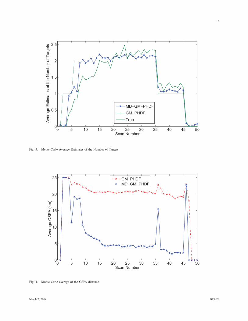
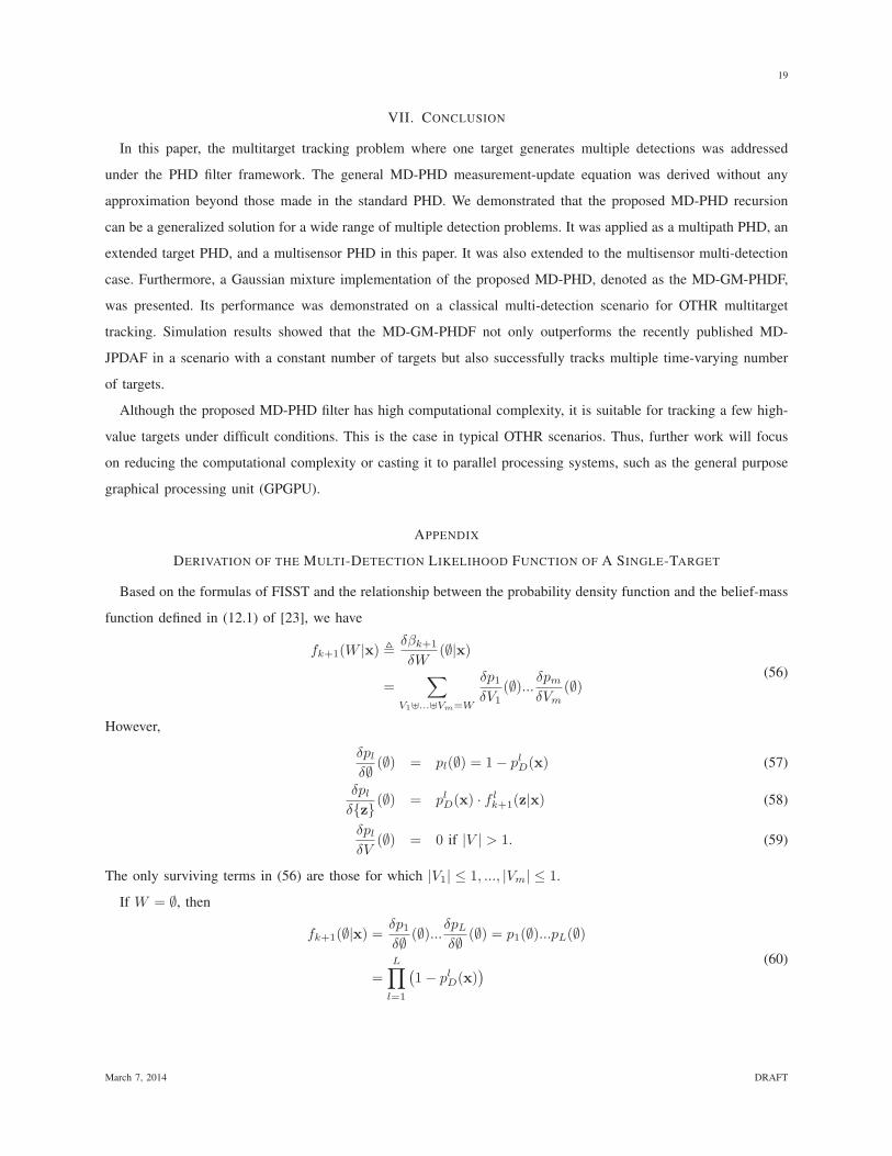
As shown in Fig. 3, the Monte Carlo averaged estimate of the number of targets from MD-GM-PHDF accurately
follows the true values after a two-scan delay. On the other hand, the GM-PHDF cannot achieve this, but it can
respond target disappearances well. Fig. 4 shows the Monte Carlo average of the optimal subpattern assignment
(OSPA) distance [39] with order p = 2 and cut-off c = 25. The peaks from the OSPA with MD-GM-PHDF at
scan index 2, 6, 36, 46, correspond to the emergence and disappearance of targets, respectively. The high OSPA
distance of GM-PHDF illustrates that the GM-PHDF cannot track the target state correctly even at scans where
target number is accurately estimated.
The results in this scenario confirm that the proposed MD-GM-PHDF can accurately estimate the dynamic target
number and improve the target state estimates when compared with the GM-PHDF.
March 7, 2014 DRAFT
18
0 5 10 15 20 25 30 35 40 45 500
0.5
1
1.5
2
2.5
Scan Number
Ave
rage
Est
imat
es o
f the
Num
ber o
f Tar
gets
MD−GM−PHDF
GM−PHDF
True
Fig. 3. Mente Carlo Average Estimates of the Number of Targets
0 5 10 15 20 25 30 35 40 45 500
5
10
15
20
25
Scan Number
Ave
rage
OS
PA
(km
)
GM−PHDFMD−GM−PHDF
Fig. 4. Monte Carlo average of the OSPA distance
March 7, 2014 DRAFT
19
VII. CONCLUSION
In this paper, the multitarget tracking problem where one target generates multiple detections was addressed
under the PHD filter framework. The general MD-PHD measurement-update equation was derived without any
approximation beyond those made in the standard PHD. We demonstrated that the proposed MD-PHD recursion
can be a generalized solution for a wide range of multiple detection problems. It was applied as a multipath PHD, an
extended target PHD, and a multisensor PHD in this paper. It was also extended to the multisensor multi-detection
case. Furthermore, a Gaussian mixture implementation of the proposed MD-PHD, denoted as the MD-GM-PHDF,
was presented. Its performance was demonstrated on a classical multi-detection scenario for OTHR multitarget
tracking. Simulation results showed that the MD-GM-PHDF not only outperforms the recently published MD-
JPDAF in a scenario with a constant number of targets but also successfully tracks multiple time-varying number
of targets.
Although the proposed MD-PHD filter has high computational complexity, it is suitable for tracking a few high-
value targets under difficult conditions. This is the case in typical OTHR scenarios. Thus, further work will focus
on reducing the computational complexity or casting it to parallel processing systems, such as the general purpose
graphical processing unit (GPGPU).
APPENDIX
DERIVATION OF THE MULTI-DETECTION LIKELIHOOD FUNCTION OF A SINGLE-TARGET
Based on the formulas of FISST and the relationship between the probability density function and the belief-mass
function defined in (12.1) of [23], we have
fk+1(W |x) � δβk+1
δW(∅|x)
=∑
V1�...�Vm=W
δp1δV1
(∅)... δpmδVm
(∅)(56)
However,
δplδ∅ (∅) = pl(∅) = 1− plD(x) (57)
δplδ{z} (∅) = plD(x) · f l
k+1(z|x) (58)
δplδV
(∅) = 0 if |V | > 1. (59)
The only surviving terms in (56) are those for which |V1| ≤ 1, ..., |Vm| ≤ 1.
If W = ∅, then
fk+1(∅|x) = δp1δ∅ (∅)... δpL
δ∅ (∅) = p1(∅)...pL(∅)
=L∏
l=1
(1− plD(x)
) (60)
March 7, 2014 DRAFT

20
If W = ∅, then
fk+1(W |x) = fk+1(∅|x) ·∑
V1�...�Vm=W
δp1
δV1(∅)... δpL
δVL(∅)∏L
l=1 (1− plD(x))
= fk+1(∅|x) ·∑
1≤l1 =... =lm≤L
δpl1
δz1(∅)... δplm
δzm(∅)
(1− pl1D(x)) · · · (1− plmD (x))
= fk+1(∅|x) ·∑
1≤l1 =... =lm≤L
m∏j=1
pljD(x) · f lj
k+1 (zj |x)1− p
ljD(x)
= L! · fk+1(∅|x) ·∑
1≤l1≤...≤lm≤L
m∏j=1
pljD(x) · f lj
k+1(zj |x)1− p
ljD(x)
(61)
where each m-tuple {l1, ..., lm} with 1 ≤ l1 = ... = lm ≤ L determines a one-to-one function τ : {1, ...,m} →{1, ..., L} by τ(j) = lj . For each m-tuple, define the association
θ : {1, ..., L} → {0, 1, ...,m}
with θ(l) = τ−1(l) if l is in the image of τ , and θ(l) = 0 otherwise. Then the m-tuple is in a one-to-one
correspondence with association θ. It is the same with those defined in Section 10.5.4 of [23]. Now, from (61) we
can get a similar form as (11) in Subsection III-B
fk+1(W |x) = fk+1(∅|x)∑θ
∏θ(l)>0
plD(x) · f l
k+1(zθ(l)|x)
1− plD(x)
=L∏
l=1
(1− plD(x)
)∑θ
∏θ(l)>0
plD(x) · f lk+1(zθ(l)|x)
1− plD(x)
(62)
REFERENCES
[1] S. S. Blackman, Multiple-Target Tracking with Radar Applications. Dedham, MA, USA: Artech House, 1986.
[2] D. Reid, “An algorithm for tracking multiple targets,” IEEE Trans. Autom. Control, vol. 24, no. 6, pp. 843–854, Dec. 1979.
[3] D. Musicki and R. Evans, “Joint integrated probabilistic data association: JIPDA,” IEEE Trans. Aerosp. Electron. Syst., vol. 40, no. 3, pp.
1093–1099, Jul. 2004.
[4] H. A. Blom and E. A. Bloem, “Interacting multiple model joint probabilistic data association avoiding track coalescence,” in Decision and
Control, Proceedings of the 41st IEEE Conference on, vol. 3, Las Vegas, Nevada, USA, 2002, pp. 3408–3415.
[5] T. Kurien, “Issues in the design of practical multitarget tracking algorithms,” in Multitarget-Multisensor Tracking: Advanced Applications,
Y. Bar-Shalom, Ed. Norwood, MA: Artech House, 1990, pp. 43–83.
[6] W. Koch and G. Van Keuk, “Multiple hypothesis track maintenance with possibly unresolved measurements,” IEEE Trans. Aerosp. Electron.
Syst., vol. 33, no. 3, pp. 883–892, Jul. 1997.
[7] R. Mahler, “Statistics 102 for multisource-multitarget detection and tracking,” IEEE J. Sel. Topics Signal Process., vol. 7, no. 3, pp.
376–389, Jul. 2013.
[8] R. L. Streit, Poisson Point Processes: Imaging, Tracking, and Sensing. New York: Springer, 2010.
[9] B. Habtemariam, R. Tharmarasa, T. Thayaparan, M. Mallick, and T. Kirubarajan, “A multiple-detection joint probabilistic data association
filter,” IEEE J. Sel. Topics Signal Process., vol. 7, no. 3, pp. 461–471, Jun. 2013.
[10] S. B. Colegrove, “Project Jindalee: From bare bones to operational OTHR,” in IEEE International Radar Conference, Alexandria,VA,
2000, pp. 825–830.
[11] M. Inggs, “Passive coherent location as cognitive radar,” IEEE Aerosp. Electron. Syst. Mag., vol. 25, no. 5, pp. 12–17, May 2010.
March 7, 2014 DRAFT

21
[12] R. Tharmarasa, M. Subramaniam, N. Nadarajah, T. Kirubarajan, and M. McDonald, “Multitarget passive coherent location with transmitter-
origin and target-altitude uncertainties,” IEEE Trans. Aerosp. Electron. Syst., vol. 48, no. 3, pp. 2530–2550, Jul. 2012.
[13] G. W. Pulford and R. J. Evans, “Probabilistic data association for systems with multiple simultaneous measurements,” Automatica, vol. 32,
no. 9, pp. 1311–1316, Sep. 1996.
[14] D. J. Percival and K. A. B. White, “Multipath track fusion for over-the-horizon radar,” in Proc. SPIE Signal Data Process. Small Targets,
vol. 3163, San Diego, CA, USA, 1997, pp. 363–374.
[15] J. Krolik and R. Anderson, “Maximum likelihood coordinate registration for over-the-horizon radar,” IEEE Trans. Signal Process., vol. 45,
no. 4, pp. 945–959, Apr. 1997.
[16] R. H. Anderson and J. L. Krolik, “Over-the-horizon radar target localization using a hidden Markov model estimated from ionosonde
data,” Radio Science, vol. 33, no. 4, pp. 1199–1213, Jul. 1998.
[17] G. W. Pulford and R. J. Evans, “A multipath data association tracker for over-the-horizon radar,” IEEE Trans. Aerosp. Electron. Syst.,
vol. 34, no. 4, pp. 1165–1183, Aug. 1998.
[18] P. W. Sarunic and M. G. Rutten, “Over-the-horizon radar multipath track fusion incorporating track history,” in Information Fusion. 3rd
International Conference on, vol. 1, Paris, France, 2000.
[19] G. Wang, X.-G. Xia, B. Root, V. Chen, Y. Zhang, and M. Amin, “Manoeuvring target detection in over-the-horizon radar using adaptive
clutter rejection and adaptive chirplet transform,” IEE Proceedings -Radar, Sonar and Navigation, vol. 150, no. 4, pp. 292–298, Aug. 2003.
[20] S. Colegrove and S. Davey, “PDAF with multiple clutter regions and target models,” IEEE Trans. Aerosp. Electron. Syst., vol. 39, no. 1,
pp. 110–124, Jan. 2003.
[21] M. Daun and W. Koch, “Multistatic target tracking for non-cooperative illumination by DAB/DVB-T,” in IEEE Int. Radar Conference,
Rome, Italy, 2008, pp. 1–6.
[22] T. Sathyan, C. Tat-Jun, S. Arulampalam, and D. Suter, “A multiple hypothesis tracker for multitarget tracking with multiple simultaneous
measurements,” IEEE J. Sel. Topics Signal Process., vol. 7, no. 3, pp. 448–460, Jun. 2013.
[23] R. Mahler, Statistical Multisource-Multitarget Information Fusion. Norwood, MA, USA: Artech House, 2007.
[24] ——, “Multitarget Bayes filtering via first-order multitarget moments,” IEEE Trans. Aerosp. Electron. Syst., vol. 39, no. 4, pp. 1152–1178,
Oct. 2003.
[25] B.-T. Vo, B.-N. Vo, and A. Cantoni, “Bayesian filtering with random finite set observations,” IEEE Trans. Signal Process., vol. 56, no. 4,
pp. 1313–1326, Apr. 2008.
[26] R. Mahler, “PHD filters for nonstandard targets, I: Extended targets,” in Information Fusion, 12th International Conference on, Seattle,
WA, 2009, pp. 915–921.
[27] ——, “The multisensor PHD filter: I. General solution via multitarget calculus,” in Proc. of the SPIE Conference on Signal Processing,
Sensor Fusion and Target Recognition, vol. 7336, Orlando, Florida, USA, 2009.
[28] D. Clark and R. Mahler, “Generalized PHD filters via a general chain rule,” in Information Fusion, 15th International Conference on,
Singapore, 2012, pp. 157–164.
[29] R. Mahler, “Second-generation PHD/CPHD filters and multitarget calculus,” in SPIE Signal and Data Process. Small Targets, San Diego,
CA, USA,, vol. 7445, San Diego,CA, Aug. 2009, pp. 74 450I–74 450I–12.
[30] G.-C. Rota, “The number of partitions of a set,” The American Mathematical Monthly, vol. 71, no. 5, pp. 498–504, May 1964.
[31] H. Torabi, J. Behboodian, and S. Mirhosseini, “On the number of partitions of sets and natural numbers,” Applied Mathematical Sciences,
vol. 3, no. 33, pp. 1635–1646, 2009.
[32] Y. Li, H. Xiao, Z. Song, R. Hu, and H. Fan, “A new multiple extended target tracking algorithm using PHD filter,” Signal Processing,
vol. 93, no. 12, pp. 3578–3588, Dec. 2013.
[33] K. Granstrom, C. Lundquist, and O. Orguner, “Extended target tracking using a Gaussian-mixture PHD filter,” IEEE Trans. Aerosp.
Electron. Syst., vol. 48, no. 4, pp. 3268–3286, Oct. 2012.
[34] B.-N. Vo and W.-K. Ma, “The Gaussian mixture probability hypothesis density filter,” IEEE Trans. Signal Process., vol. 54, no. 11, pp.
4091–4104, Nov. 2006.
[35] K. Panta, D. E. Clark, and B.-N. Vo, “Data association and track management for the Gaussian mixture probability hypothesis density
filter,” IEEE Trans. Aerosp. Electron. Syst., vol. 45, no. 3, pp. 1003–1016, Jul. 2009.
March 7, 2014 DRAFT

22
[36] R. Sithiravel, X. Chen, R. Tharmarasa, B. Balaji, and T. Kirubarajan, “The spline probability hypothesis density filter,” IEEE Trans. Signal
Process., vol. 61, no. 24, pp. 6188–6203, Dec. 2013.
[37] N. Whiteley, S. Singh, and S. Godsill, “Auxiliary particle implementation of probability hypothesis density filter,” IEEE Trans. Aerosp.
Electron. Syst., vol. 46, no. 3, pp. 1437–1454, Jul. 2010.
[38] Y. Bar-Shalom, X. R. Li and T. Kirubarajan, Estimation with Applications to Tracking and Navigation. NY, USA: Wiley, 2001.
[39] D. Schuhmacher, B.-T. Vo, and B.-N. Vo, “A consistent metric for performance evaluation of multi-object filters,” IEEE Trans. Signal
Process., vol. 56, no. 8, pp. 3447–3457, Aug. 2008.
March 7, 2014 DRAFT