1

An image processing system for qualitative and quantitative volumetric

analysis of brain images

†Alberto F. Goldszal, Ph.D.

§Christos Davatzikos, Ph.D.

*†Dzung L. Pham, M.S.E.

‡Michelle X. H. Yan, Ph.D.

§R. Nick Bryan, M.D., Ph.D.

†Susan M. Resnick, Ph.D.

†Laboratory of Personality & Cognition, Gerontology Research Center, National Institute on

Aging, National Institutes of Health, 5600 Nathan Shock Drive, Baltimore, MD 21224 USA

§ Department of Radiology and Radiological Science, The Johns Hopkins University School of

Medicine, 600 N. Wolfe St., Baltimore, MD 21287 USA

* Department of Electrical and Computer Engineering, The Johns Hopkins University, Baltimore,

MD 21218 USA

‡ Department of Psychiatry, University of Pennsylvania, Philadelphia, PA 19104 USA

2

Blinded Title Page:

An image processing system for qualitative and quantitative volumetric

analysis of brain images

3

Proposed running head:

Analyzing global and regional brain volumes

Correspondence author:

Alberto F. Goldszal, Ph.D.

National Institutes of Health

National Institute on Aging, GRC, LPC

5600 Nathan Shock Drive, Suite 2C20

Baltimore, MD 21224-6825 USA

Tel: (410) 558-8624

Fax: (410) 558-8108

Email: goldszal@nih.gov

4

ABSTRACT

In this work, we developed, implemented and validated an image processing system for

qualitative and quantitative volumetric analysis of brain images. This system allows the

visualization and quantitation of global and regional brain volumes. Global volumes were obtained

via an automated adaptive Bayesian segmentation technique which labels the brain into white

matter, gray matter and cerebrospinal fluid. Absolute volumetric errors for these compartments

ranged between 1–3% as indicated by phantom studies. Quantitation of regional brain volumes was

performed through normalization and tessellation of segmented brain images into the Talairach

space with a 3-D elastic warping model. Retest reliability of regional volumes measured in

Talairach space indicated errors of less than 1.5% for the frontal, parietal, temporal and occipital

brain regions. Additional regional analysis was performed with an automated, hybrid method

combining a region-of-interest approach and voxel-based analysis named Regional Analysis of

Volumes Examined in Normalized Space (RAVENS). RAVENS analysis for several subcortical

structures showed good agreement with operator-defined volumes. This system has sufficient

accuracy for longitudinal imaging data and is currently being used in the analysis of neuroimaging

data of the Baltimore Longitudinal Study of Aging (BLSA).

5

INTRODUCTION

The precise quantification of structural changes that occur in the brain with aging or disease

has been an area of active research in neuroimaging for many years. To accurately characterize

brain structure and any anatomic changes which may occur over time, and to correlate such

anatomical changes with concurrent physiological or cognitive changes, we developed,

implemented, and validated a set of imaging tools capable of capturing subtle longitudinal changes

in the regional and global volumetric structure of the brain. We tested this system on cross-

sectional and longitudinal magnetic resonance (MR) imaging data acquired as part of the

neuroimaging study of participants in the Baltimore Longitudinal Study of Aging (BLSA) (1). The

main goal of this image processing system is to measure the magnitude, rate and regional pattern of

longitudinal changes in the brain. Future applications are extensible to functional neuroimaging

data. All system components have known accuracy and errors, and thus, the overall system

accuracy can be estimated.

The application of an image processing system within a large scale longitudinal brain

imaging study has posed difficulties in the development, implementation and validation of the

different components. Methods typically employed in cross-sectional studies do not have sufficient

sensitivity to detect more subtle longitudinal changes. Most studies focusing on the volumetric

analysis of the brain deal with cross-sectional data and seek the measurement of part of or the total

volume of a structure or region of interest (2–6). Although the notion that imaging studies

employing quantitative volumetric methods potentially yield more accurate and less biased results

than qualitative studies is widely accepted, validating this assumption can be difficult and time-

consuming. Quantitative neuroanatomic methods may range from manual, local operations in 2-D

images (7) to automated, 3-D model-based brain volume estimations (2, 8) to continuous,

automated, 3-D volumetric measurements based on probabilistic atlases of neuroanatomy (9–12).

Detailed cortical parcellation techniques have been developed (13), but they are extremely laborious

and time-consuming. In addition, these approaches usually depend on subjective criteria, leading to

6

difficulties in establishing reliability and validity. Finally, an extensive literature exists on

stereological methods (14, 15), which, however, are suitable only for volumetric measurements of

large partitions; detecting small local changes by fine sampling would require a prohibitive amount

of work.

In our case, we are interested in accurately, reliably and automatically measuring the total

volumes of structures and regions in the brain. We are particularly concerned with the ability to

capture small structural brain changes which may occur over time at global and regional (local)

levels. The quantitative methods used in our system include the acquisition of 3-D high-resolution

MR spoiled grass (SPGR) images, pre-processing of the data, image segmentation, normalization

and regional volumetric analyses including the volumetric quantification of MR images within a

stereotaxic coordinate system.

At the center of this image processing system are the segmentation and normalization

techniques. Our segmentation approach (16) has the ability to adapt to shading artifacts caused by

non-uniformities in the radiofrequency (RF) field during image acquisition. Shading artifacts,

which occur in nearly all MR images, cause voxel intensities of the same tissue class to vary over

the image domain. These artifacts may be corrected prior to the image segmentation step (17–20) or

their correction may be embedded within the segmentation procedure (16, 21–23). In the former

case, an algorithm first compensates for the shading artifact, then the image is segmented by one of

the several available segmentation techniques (24). In the latter group, the intensity

inhomogeneities are compensated simultaneously with image segmentation. In either case, not

compensating for the shading artifacts might severely limit the accuracy of any segmentation

technique operating on MR images. In addition to shading artifacts, our approach is also very

robust to poor soft tissue contrast, low signal-to-noise ratio and partial volume effects.

The segmentation allows quantitative measures of global changes in the brain, however,

additional tools are necessary to measure the local magnitude and regional pattern of longitudinal

changes in the brain. To quantify regional volumes, we examine the brain images within a standard

stereotaxic space, the Talairach coordinate space (25), after spatially normalizing all images for

7

overall shape differences. Several methodologies for spatial normalization of brain images have

been proposed in the literature (25–34). Our approach is based on a geometric deformable model,

coded in the STAR algorithm, which uses a surface-based elastic warping transformation to bring

two 3-D images into registration (35, 36). This technique has superior performance and better

accuracy than other normalization methods which are based on a piecewise linear Talairach

transformation (2) or normalization approaches employed by statistical parametric mapping (SPM)

(32) because it utilizes several explicit features, e.g., the ventricular boundary, as well as the outer

cortical surface, to drive the elastic transformations. The use of the ventricular boundaries and

cortical features is particularly critical in the presence of atrophy, a situation common in the elderly.

For the regional analysis in stereotaxic space, the segmented data are tessellated into the

1,056 Talairach boxes (25). This method yields an accurate and reliable approach for quantitation

of large brain regions; however, due to the discrete nature of the Talairach boxes, it is not suitable

for smaller regions or individual brain structures. For the quantitation of smaller brain regions, we

employ a hybrid procedure which combines the stability of a region-of-interest (ROI) approach

with the spatial resolution of a voxel-based method. We refer to this alternate procedure as

Regional Analysis of Volumes Examined in Normalized Space, or RAVENS.

MATERIALS AND METHODS

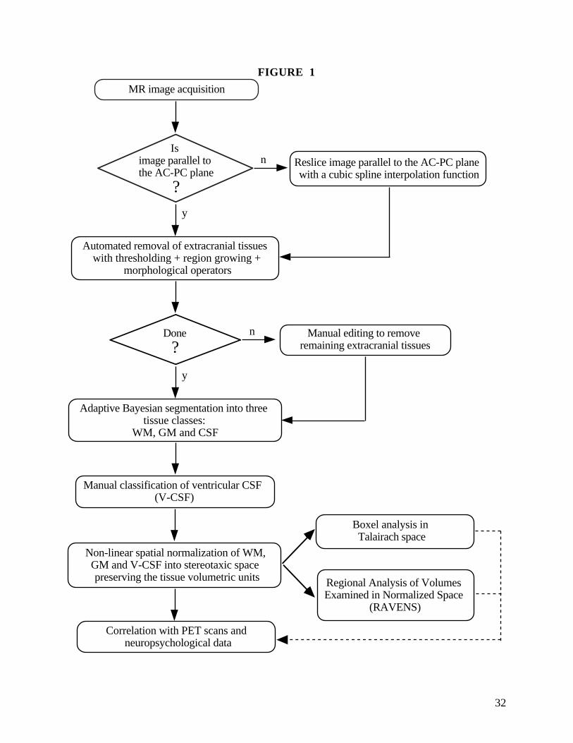
System Overview. Image analysis is comprised of several steps including reslicing of the data,

removal of extracranial tissues, segmentation of different tissue types, normalization to a standard

coordinate space, and regional quantitative analysis. A schematic diagram illustrating the overall

procedure is shown in Figure 1. In this section, we describe each component in greater detail.

MRI Acquisition . While the main goal of this paper is to present an image analysis

methodology, we tested our protocols on a small sample of elderly subjects — a subset of the

participants in the Baltimore Longitudinal Study of Aging (1). All subjects in this study were

8

scanned with a GE Signa 1.5 T scanner (GE Medical Systems, Waukesha, WI) employing a T1-

weighted Spoiled GRASS (SPGR) pulse sequence. The parameters of the SPGR sequence were

TR = 35 ms, TE = 5 ms, flip angle = 45°, image size = 256 x 256 x 124 voxels, and voxel size =

0.9375 x 0.9375 x 1.5 mm3.

Image Reformatting. After acquisition, the images were resliced parallel to the AC-PC plane

using (i) the correctional angles for roll, yaw, and pitch determined interactively, and (ii) cubic

splines for interpolation of the data running on a Silicon Graphics Indigo2 high-impact workstation

(Silicon Graphics Inc., Mountain View, CA).

Removal of Extracranial Tissues. An important pre-processing step is the removal of

extracranial tissues because our segmentation technique labels the entire brain into three global

compartments: WM, GM and CSF. Removal of extracranial tissues is also important for the

stereotaxic normalization which is based on the brain boundaries as opposed to the skull contour.

Removal of extracranial tissues was accomplished by a sequential application of

morphological operators, thresholding, seeding, region growing, and manual editing. First, a

morphological erosion with a spherical structuring element (default radius = 2 mm) detaches the

brain tissue from the surrounding dura. Next, a 3-D seeded region growing extracts the brain

tissue. Finally, a 3-D morphological dilation with a spherical structuring element (default radius =

4 mm) recaptures the tissue lost in the erosion step. Note that the radius of the sphere used in the

dilation is larger than the one used in the erosion in order to guarantee that no brain tissue is lost

either due to the manual thresholding or to the erosion. In addition, whenever users assign a

narrow threshold range, holes may be created inside the brain region. As long as these holes are

not connected to the image background, they are automatically recognized as brain regions and

filled with the original voxel values. If needed, bridges are placed to sever any connection of these

holes with the background.

9

This automated step takes less than a minute (running on a SGI Indigo2) to generate a

“deskulled” image set. A limitation of this method for pre-processing SPGR images is that an

undetermined amount of sulcal CSF is removed because the CSF-dura interface is difficult to

determine reliably with the SPGR pulse sequence. Thus, sulcal CSF cannot be estimated reliably

from our SPGR images. Typically, the automated step generates an image which is adequate for

many image processing operations, such as registration and 3-D rendering. However, for a

quantitative volumetric analysis of brain images, some manual editing was necessary to extract the

sagittal sinus anteriorly and posteriorly, to eliminate extracranial tissues mesial to the temporal

lobes, and to remove portions of the dura posteriorly. In addition, prior to the segmentation step,

we manually edited out the cerebellum and brainstem due to concerns about the adequacy of our

segmentation algorithm to accurately label these regions and our emphasis on quantitative analysis

of the cerebrum. Figures 2A–C illustrate, for a single brain slice, the complete removal process of

extracranial tissues.

Quantitation of Global Brain Volumes. Following the removal of extracranial material, each

voxel in the brain-extracted image is labeled into WM, GM and CSF using a 3-D generalization of

the method developed by Yan et al. (16). This technique segments single- or multi-spectral brain

images into m-different tissue types where, in our study, m = 3 for WM, GM and CSF. Each

scalar-valued image (e.g., a MR SPGR volume) is modeled as a collection of regions with slowly

varying intensity, described by B-spline functions, plus white Gaussian noise. Spatial smoothness

of the segmentation is obtained by modeling voxel dependencies by a 3-D, second order Markov

Random Field (MRF).

The algorithm maximizes the a posteriori probability jointly over tissue types and mean

intensities in an iterative and adaptive fashion. For each iteration, it estimates (i) the mean

intensities for each tissue type via a least squares fitting of the B-spline function, and (ii) the tissue

type regions modeled by a MRF. By increasing the number of control points of the B-spline

10

functions, the algorithm slowly adapts to regional intensity variations which, in the case of MR

images, may be caused by shading artifacts due to MR field inhomogeneities.

The segmentation algorithm is fully automated. As an initial step, the algorithm pre-

segments the data with a k-means clustering technique which groups the voxels in the image into k

clusters through the minimization of the total inter-cluster variance (a maximum likelihood

estimation). The result of the pre-segmentation is then used as an initial classification for the

adaptive and iterative model. After the automated segmentation into WM, GM and total CSF, the

ventricular CSF (V-CSF) was determined by manually drawing a crude ROI to eliminate any CSF

falling outside the ventricular system. This ROI served as a mask within which CSF voxels on the

segmented image were reclassified as V-CSF.

Image Normalization . The segmented images provide global volumetric measurements of the

total amount of WM, GM and V-CSF. To quantify regional brain volumes, however, the images

were examined within a standard stereotaxic space, the Talairach reference space (25), after

spatially normalizing all images for global morphological differences. The spatial normalization of

the images was performed using the STAR algorithm detailed in (35, 36).

Briefly, a parametric representation of the outer boundary of the brain was first determined

from the skull-stripped images, using the deformable surface algorithm developed by Davatzikos

(36). Based on this representation, a map from the outer boundary of each subject’s brain to the

brain of the Talairach atlas (25) was obtained. This map was determined by maximizing the

similarity of geometric characteristics between the subject’s brain and the brain of the atlas. For

example, the outer edges of the inter-hemispheric and Sylvian fissures, which have high curvature,

are recognized and matched by the algorithm.

Subsequently, each image was elastically warped to satisfy the outer cortical map,

accounting for the overall shape differences in the subjects’ brains. Additionally, variability in

ventricular size was accounted for using a uniform strain within the ventricles. This procedure

allowed their contraction corresponding to volumetric differences between each subject’s ventricles

11

and the ventricles in the atlas. After this gross volumetric correction, a force field applied to the

ventricular boundaries brought them into register with the ventricular boundaries in the atlas.

Ventricular registration is an important step in our normalization procedure because we are imaging

older subjects who, typically, have enlarged ventricles compared with younger subjects. The rest

of the brain tissue was deformed according to the equations governing the deformation of an elastic

solid.

Another important characteristic of our spatial normalization procedure is the preservation

of the tissue volumetric units in stereotaxic space, rather than the tissue density as is customary in

many spatial normalization methods (2, 32). Therefore, the total volumes of WM, GM and V-CSF

are the same before and after normalization. It is important to preserve the tissue volumetric units to

permit quantitative analyses in stereotaxic space. For example, a volumetric difference between the

two hemispheres would otherwise be eliminated after normalization to the symmetric Talairach

atlas.

Quantitation of Regional Brain Volumes. The regional quantitative analysis is performed

by two distinct methods: the “Boxel” counting method and the RAVENS method. Both approaches

quantify brain regions in stereotaxic space and are based on the previously segmented and

normalized images. The major differences between the regional quantitation methods are related to

resolution and visualization issues. The Boxel method is adequate for quantitation of large

compartments like the frontal, temporal, parietal and occipital brain regions (2). The method is

fully automated and visualization is not required. The RAVENS approach takes full advantage of

visual information and mapping techniques and is best suited for quantitation and visualization of

smaller brain regions like the caudate nucleus, the lenticular nucleus, the temporal horns, and

potentially, specific cortical ROIs. These regions are not individually labeled by the global

segmentation method nor quantified by the Boxel approach. Additionally, the RAVENS method is

more flexible and takes advantage of the image’s full resolution through a voxel-based analysis.

The method can operate in an automated or interactive mode.

12

The Boxel Method — Tissue Distributions in Talairach Space and Box Analysis. Following

normalization, the segmented images were tessellated into 1,056 boxes, as described in (25). The

total amounts of WM, GM and V-CSF were measured for each box. These 1,056 measurements

could in principle be compared individually across subjects; however, such comparisons would be

meaningful only if the normalized images were in perfect register. In practice, this is not the case,

due to residual inter-individual variability after normalization. Therefore, measurements at the box

level are likely to have higher variance across individuals, which would reduce the statistical

significance of morphological changes or differences observed. In addition, each box may include

several anatomic regions, limiting the utility of data based on individual boxes.

The individual boxes were thus grouped into larger brain compartments, as defined and

validated by Andreasen and colleagues (2). Specifically, we defined four major compartments

corresponding to the frontal, temporal, parietal and occipital lobes. Then, after tessellating a

segmented brain image into the Talairach space, regional quantitation is obtained by counting the

volumes for each tissue type, i.e., WM, GM and V-CSF, within each of the four lobes for each

hemisphere.

RAVENS — Regional Analysis of Volumes Examined in Normalized Space. The Boxel method

provides a low resolution “boxelated” description of tissue distributions in Talairach space. The

RAVENS technique yields a more accurate and flexible analysis that combines the stability and

flexibility of an ROI approach with the spatial resolution of a voxel-based method.

The normalization of the images into the Talairach space causes a deformation of the

original image morphology; however, applying the RAVENS method, the tissue volumes are

preserved by coding them as intensity-based maps. As shown in Figure 3A–D, brain regions

which expanded during the normalization step will look darker than their original counterparts

because the same amount of tissue was spread over a larger area. Similarly, regions which were

decreased in size will look proportionally brighter. Note that after normalization, the shape and size

13

of both ventricles are similar (as expected) and the differences in volumes are coded as intensity-

based maps.

Once the segmented tissue distributions are stereotaxically normalized, they may be

averaged to generate mean images for groups or processed individually for longitudinal analyses.

Typically, as illustrated in Figure 4A–C, we generate average images over samples of interest and

display them as intensity-based maps. Besides being able to carry out quantitative analyses in

normalized space, these displays allow for scale-space analysis (by allowing different degrees of

blurring) and provide a representation which can be directly correlated with other imaging

modalities such as normalized PET scans.

The quantitative analysis of brain structures and regions with the RAVENS maps may be

performed in two different ways: (i) a free-hand ROI may be drawn directly on a RAVENS map as

illustrated in Figure 5A; integration of the RAVENS map within this ROI yields the volume of the

underlying structure. Or, (ii) as illustrated in Figure 5B, a brain structure may be chosen in a co-

registered digital brain atlas; this atlas’ structure is then overlaid onto the RAVENS map, marking a

3-D region which is integrated through all slices yielding the volume of the structure being studied.

This method is particularly attractive to us since many brain regions have already been delineated

and defined in a digital stereotaxic atlas of neuroanatomy (37), allowing automated processing of

many regions. The volumetric accuracy of this method becomes mainly a function of the global and

local registration precision between the digital atlas and the RAVENS maps.

ASSESSMENT OF RELIABILITY AND VALIDITY

Removal of Extracranial Tissues. Since the complete removal of extracranial tissues

involved manual editing by an operator, interoperator differences were examined to assess how

distinct operators would affect the stripping process. For this test, fourteen images were initially

processed with the automated part of the skull stripping method and then manually edited,

independently by two operators, for any extracranial tissues still present in the images. Finally,

14

these two sets of images were segmented and the volumes of the white matter and gray matter

compartments compared by t-test.

Image Segmentation — Phantom. To assess the accuracy of the adaptive Bayesian method

and to compare it against other segmentation techniques, we created the 3-D digital brain phantom

depicted in Figure 6. The overall shape of the phantom and the volume of its three major

compartments — WM, GM and CSF — are based on a segmented SPGR image of a 72 year old

subject. In this case, the segmentation involved a simple thresholding technique which was

complemented by manual outlining. The matrix size of the phantom is 256 x 256 x 72 voxels with

each voxel measuring 0.9375 mm2 x 1.5 mm and having 8-bits of depth. This image set serves as

our standard reference, with known volumes for WM, GM and CSF.

A number of parameters may be modified in the phantom to create a realistic looking image

(Figure 6A) which simulates the appearance and characteristics of an older brain. These parameters

include: mean intensity values, noise, magnetic field inhomogeneities and partial volume effects.

The specific parameters employed in our validation studies were determined from MRI scans of ten

older individuals aged 59–84 years. Based on these images, mean intensity values of the phantom

were fixed at 112.08, 87.53, and 35.00 for the WM, GM and CSF, respectively. The standard

deviation of the superimposed Gaussian noise was set to 6.0. The 3-D linear shading which

simulated magnetic field inhomogeneities was 7% in each direction. Finally, the partial volume

averaging effect of the MR acquisition was simulated substituting each point in the final image by a

weighted average in its 6-connected 3-D neighborhood.

Results for the adaptive Bayesian method (Figure 6B) were compared with: a Gaussian

clustering method, a n-nearest neighbors classifier, and a neural networks technique all

implemented in the Analyze biomedical image analysis package (38); a region growing method and

a multiple thresholding technique implemented in the MEDx radiological image processing

software (Sensor Systems Inc., Sterling, VA); and a standard fuzzy c-means algorithm (24).

15

Short-Term Reliability . To assess the short-term reliability of our quantitative approach, three

subjects had repeated SPGR scans separated by approximately 30 minutes with the subjects being

removed from the scanner and repositioned between the two SPGR acquisitions. The images were

volumetrically acquired, pre-processed to remove extracranial tissues, and segmented into WM,

GM and V-CSF.

Longitudinal Stability . To assess the longitudinal or long-term stability of our approach, we

examined data from ten BLSA subjects, who had been imaged at times t and t+1 year. The ten

subjects ranged in age from 59–84 years (mean, 72.4 years ± 10.7). SPGR images were acquired

approximately one year apart. These images were pre-processed and segmented into WM, GM and

V-CSF. However, unlike the short-term reliability study previously described, for a single subject,

any observed differences in the volumes of WM, GM and V-CSF compartments between times t

and t+1 year, do not necessarily reflect inconsistencies or errors in the image analysis protocol

employed. During a period of one year, it is conceivable that true anatomical changes may take

place, altering the volumes of the WM, GM and/or V-CSF. The possibility of true longitudinal

brain changes may be particularly relevant for older subjects. Thus, any differences between

volumetric measurements at times t and t+1 year confound measurement errors and true

longitudinal changes, and reflect upper-bound estimates of the measurement error.

Regional Brain Volumes — Boxel Analysis. Reliability of the Boxel analysis was

assessed using the images from the three subjects with repeated SPGR scans separated by 30

minutes. Following segmentation into WM, GM and V-CSF, the images were tessellated into the

Talairach space and regional tissue distributions computed for the frontal, parietal, temporal and

occipital regions. Comparisons of the regional tissue distributions between times t and t+30

minutes provide measures of repeatability.

16

RAVENS. To illustrate and validate the application of the RAVENS approach for visualization

and quantitation of regional brain volumes, average maps were created for the sample of ten

subjects aged 59–84 years. The RAVENS method was applied to these maps and three brain

regions were quantified: the caudate nucleus, the lenticular nucleus, and the temporal horns.

Validation of this approach was accomplished via manual outlining (independently by two

operators) and volume computation for the three structures using the original MR images. These

volumes were then compared to those obtained with the RAVENS method.

RESULTS

Removal of Extracranial Tissues. The interoperator reliability test revealed that there were

only small differences in the manual editing between the two trained operators. For the fourteen

image sets evaluated, the average within subject difference between raters was -0.02% ± 1.37 for

WM and 0.46% ± 0.88 for GM. Correlations were greater than 0.99 for both measures. Finally,

paired t-test comparisons yielded no significant differences between raters.

Quantitation of Global Brain Volumes — Phantom. The results for the comparison of

different segmentation methods are presented in Table 1. The adaptive Bayesian technique yielded

absolute volumetric errors on the order of 1–3% for each individual compartment and 0.43% for

the total brain tissue volume. In addition, the adaptive Bayesian method presented better overall

accuracy for segmentation of the WM, GM and CSF volumes of simulated MR SPGR images

when compared against all tested approaches. Finally, we also tested the accuracy of our

segmentation approach on a different phantom developed by A. C. Evans and colleagues (39) at

the Montreal Neurological Institute (http://www.bic.mni.mcgill.ca), obtaining very similar results.

It is also observed that the fuzzy c-means algorithm, a very popular algorithm used in brain

image segmentation, presented a slightly better result in the segmentation of the CSF compartment,

but less accurate measurement of WM and GM volumes. We believe that the adaptive Bayesian

17

technique presented better overall segmentation results mainly due to its ability to adapt to local

image intensity variations caused by shading artifacts due to MR field inhomogeneities.

Short-Term Reliability . The short-term reliability assessment for the three subjects showed

that the average absolute volumetric differences between measures at times t and t+30 minutes for

WM, GM, total brain tissue volume, and V-CSF, calculated as |((Scan2 – Scan1)/Scan1)|*100%,

were 0.75% ± 0.38, 0.71% ± 0.62, 0.31% ± 0.37, and 0.87% ± 0.93, respectively.

Longitudinal Stability . Longitudinal changes in volumes were calculated as ((Year2 –

Year1)/Year1)*100% for the ten subjects studied at times t and t+1 year. The average longitudinal

volumetric differences for WM, GM, total brain volume, and V-CSF were -0.46% ± 2.34, -0.03%

± 1.08, -0.26% ± 1.09, and 3.52% ± 2.21, respectively. Correlations between measurements at

time t and time t+1 year for WM, GM, total brain volume, and V-CSF were, respectively, 0.98,

0.99, 1.00, and 1.00.

Quantitation of Regional Brain Volumes — Boxel Analysis. The results for the Boxel

approach are summarized in Table 2 and indicate good repeatability of the overall method. We also

used these data to compare the WM, GM, total brain, and V-CSF volumes yielded by the Boxel

method and our global segmentation technique. The results showed no volumetric differences

between the global segmentation results and Boxel method for the above mentioned compartments.

Therefore, as predicted from our design, the normalization and tessellation procedures preserve the

tissue volumetric units in stereotaxic space.

RAVENS. The mean volumes and standard deviations found using the manual tracing approach

and the RAVENS plus atlas method are presented for the temporal horns, caudate nucleus and

lenticular nucleus in Table 3. For all three structures, paired t-tests indicated no significant

differences between operator-determined volumes and those calculated using RAVENS. For the

18

caudate nucleus, the correlations between operator A and operator B, operator A and RAVENS

method, and operator B and RAVENS method were, respectively, 0.90, 0.84 and 0.84. For the

lenticular nucleus, these correlations were 0.92, 0.85 and 0.79, respectively. Finally, for the

temporal horns, the correlations were 0.99, 0.95 and 0.97, respectively. Intraclass correlations

among the three estimates were 0.86, 0.86, and 0.95 for the caudate, the lenticular nucleus, and

the temporal horns, respectively. Note that it was necessary for the two operators to train on

several series of image data sets to achieve acceptable interoperator agreement.

DISCUSSION

In this paper, we presented and validated an image processing system for qualitative and

quantitative volumetric analysis of MR images of the brain. The development of the different

system components was motivated by our need for an accurate and reliable system capable of

analyzing cross-sectional and longitudinal data. The application of this image processing system

within the framework of a large scale longitudinal study posed unique difficulties in the

development, implementation and validation of the different system components. A general goal of

our system is to reliably and accurately analyze and quantify large amounts of volumetric data over

a period of years. Specifically, based on the analysis of structural MR data, we want to measure

the magnitude, rate and regional pattern of longitudinal changes in the brain. We achieved these

goals by designing a system with the following basic characteristics: the accuracy and errors of the

individual system components are measurable and known, providing an estimate of the overall

system accuracy; the system must be efficiently implemented since large amounts of data are being

processed; whenever possible, methods are automated without compromising their accuracy;

manual handling of the data is kept at a minimum, and the variability introduced by different

operators, when necessary, is measured. Additionally, the MR data are processed in a manner

which permits correlation and combination with external measures (e.g., neuropsychological

assessments of memory and cognition) and/or other imaging modalities such as PET and other

19

functional neuroimaging measures. Furthermore, the methods were adapted and optimized to

manipulate data sets from older subjects who typically have enlarged ventricular systems and

greater degree of brain atrophy.

Our imaging system was divided into five major components or steps: acquisition of the

MR data, image pre-processing, global segmentation, stereotaxic normalization and regional

volumetric analyses which, in turn, were composed of the Talairach boxes counting method (the

‘Boxel’ method) and a newly proposed RAVENS method.

Our assessment of the error introduced by trained operators during the image pre-

processing step indicated that interoperator variability is less than 1% of WM, GM and total brain

volumes. Errors in the tissue labeling ranged between 1–3% for WM, GM and CSF as shown by

phantom studies. This accuracy indicates that we have sufficient sensitivity to detect longitudinal

volumetric changes greater than 2 to 3% for individual measures of WM, GM and CSF.

Furthermore, this technique has the ability to detect longitudinal volumetric changes on the order of

0.5% for the total brain tissue volume. The adaptive Bayesian segmentation technique does better

than other segmentation schemes to which it was compared. This is in part due to this technique’s

refined modeling of the problem and its improved ability to adapt to shading artifacts caused by

local inhomogeneities in the magnetic field gradients of the MR scanner. The accuracy of the

adaptive Bayesian approach for segmentation of SPGR images is a significant advance, as poor

results with prior methods have led to reluctance in using these high resolution images for

quantification of WM and GM volumes. This segmentation technique also demonstrated good

longitudinal stability. However, establishing actual long-term retest reliability is difficult because

true changes in brain structure may occur. Our experiments provide a lower-bound estimate of

longitudinal reliability since volumetric measurements over a period of one year confound

methodological errors and true anatomical changes.

During normalization, the registration of the ventricular boundaries was an important

consideration when processing brain images of older subjects who, typically, have enlarged

ventricles and sulci compared with younger subjects. The normalization of the segmented data,

20

preserving the true volumetric units of the tissue distributions, allowed quantitation within

Talairach space. The Boxel approach showed excellent repeatability and short-term stability.

Regional absolute volumetric differences between scan-rescan were, in general, less than 1% for

all four brain regions. Although our implementation represents a significant improvement over

existing methods, it still has limitations associated with the existence of multiple anatomical regions

within the individual boxes.

An alternative way to measure regional tissue distributions is the RAVENS approach which

allows us to quantify and visualize segmented brain images in normalized space. Particularly, we

are able to analyze brain structures which are not quantifiable by the global segmentation method or

the Talairach boxes counting approach due to limitations in the accuracy and resolution of these

techniques. When used in conjunction with a co-registered digital atlas of neuroanatomy, the

RAVENS method is as reliable and accurate as a trained operator for the detection and volume

computation of certain brain structures. In addition, the RAVENS approach has the advantage of

computing ROI volumes faster and automatically, substantially increasing speed of image

processing. Typically, this approach can be used to provide fast processing and efficient screening

of large amounts of neuroimaging data. For instance, one can compute the volumes of several

different structures and focus further analysis on those structures which revealed greater changes,

i.e., those “highlighted” brain structures can be later analyzed with more elaborate and time-

consuming techniques.

Although the RAVENS method is capable of handling smaller structures and has better

anatomical specificity, it needs validation in the quantification of smaller brain structures like the

hippocampus and specific cortical ROIs. Future methodological improvements also include

refinements in the registration of the RAVENS maps and the digital atlas of neuroanatomy. With a

larger number of natural landmarks being automatically recognized and matched during the

normalization, residual registration errors tend to decrease, therefore, improving the quantification

accuracy of selected brain structures. Finally, extension of these methods to other imaging

acquisition protocols and imaging modalities is also being pursued.

21

ACKNOWLEDGMENTS

This work was supported in part by NIH contract NIH-AG-93-07. Christos Davatzikos,

Ph.D., was supported in part by a Whitaker Foundation research grant. The authors would like to

express their gratitude to Cindy B. Quinn, R.N., for helping with several manual image processing

tasks and Michael Unser, Ph.D., for providing the spline interpolation algorithm.

22

REFERENCES

1. Shock NW, Greulich RC, Andres R, et al. Normal human aging: the Baltimore Longitudinal

Study of Aging. U.S. Public Health Service publication no. NIH 84-2450. Washington, D.C.:

U.S. Government Printing Office, 1984.

2. Andreasen NC, Rajarethinam R, Cizadlo T, et al. Automatic atlas-based volume estimation of

human brain regions from MR images. J Comput Assist Tomogr 1996;20(1):98–106.

3. Jack JCR, Twomey CK, Zinsmeister A, et al. Anterior temporal lobes and hippocampal

formations: normative volumetric measurements from MR images in young adults. Radiology

1989;172:549–54.

4. Kertesz A, Polk M, Black SE, Howell J. Sex, handedness, and the morphometry of cerebral

assymmetries on magnetic resonance imaging. Brain Res 1990;530:40–8.

5. Shenton ME, Kikinis R, Jolesz FA, et al. Abnormalities of the left temporal lobe and thought

disorder in schizophrenia: a quantitative magnetic resonance imaging study. N Engl J Med

1992;327:604–12.

6. Andreasen NC, Ehrhardt JC, Swayze VW, et al. Magnetic resonance of the brain in

schizophrenia: the pathophysiological significance of structural abnormalities. Arch Gen Psychiatry

1990;47:35–44.

7. Reiss AL, Faruque F, Naidu S, et al. Neuroanatomy of Rett syndrome: a volumetric imaging

study. Ann Neurol 1993;34:227–234.

23

8. Collins DL, Holmes CJ, Peters TM, Evans AC. Automatic 3-D model-based neuroanatomical

segmentation. Hum Brain Map 1995;3:190–208.

9. Evans AC, Kamber M, Collins DL, MacDonald D. An MRI-based probabilistic atlas of

neuroanatomy. In: Shorvon SD, et al. Ed. Magnetic resonance scanning and epilepsy. New York:

Plenum Press, 1994:263–274.

10. Thompson PM, MacDonald D, Mega MS, Holmes CJ, Evans AC, Toga AW. Detection and

mapping of abnormal brain structure with a probabilistic atlas of cortical surfaces. J Comput Assist

Tomogr 1997;21(4):567–581.

11. Haller JW, Christensen GE, Joshi SC, Newcomer JW, Miller MI, Csernansky JG, Vannier

MW. Hippocampal MR imaging morphometry by means of general pattern matching. Radiology

1996;199:787–791.

12. Davatzikos C, Vaillant M, Resnick S, Prince JL, Letovsky S, Bryan RN. A computerized

approach for morphological analysis of the corpus callosum. J Comput Assist Tomogr

1996;20:88-97.

13. Rademacher J, Galaburda AM, Kennedy DN, Filipek PA, Caviness VS Jr. Human cerebral

cortex: localization, parcellation, and morphometry with magnetic resonance imaging. J Cogn

Neurosci 1992;4(4):352–374.

14. Roberts N, Cruz-Orive LM, Reid NMK, Brodie DA, Edwards RHT. Unbiased estimation of

human body composition by the Cavalieri method using magnetic resonance imaging. J

Microscopy 1993;171:239–253.

24

15. Pakkenberg B, Boesen J, Albeck M, Gjerris F. Unbiased and efficient estimation of total

ventricular volume of the brain obtained from CT scans by a stereological method. Neuroradiology

1989;31:413–417.

16. Yan MXH, Karp JN. An adaptive Bayesian approach to three-dimensional MR brain

segmentation. In Proceedings of XIVth International Conference on Information Processing in

Medical Imaging 1995; pp 201–213.

17. Dawant BM, Zijidenbos AP, Margolin RA. Correction of intensity variations in MR images for

computer-aided tissue classification. IEEE Trans Med Imag 1993;12:770–781.

18. Meyer CR, Peyton HB, Pipe J. Retrospective correction of intensity inhomogeneities in MRI.

IEEE Trans Med Imag 1995;14:36–41.

19. Johnston B, Atkins MS, Mackiewish B, Anderson M. Segmentation of multiple sclerosis

lesions in intensity corrected multispectral MRI. IEEE Trans Med Imag 1996;15:154–169.

20. Lim KO, Pfefferbaum A. Segmentation of MR brain images into cerebrospinal fluid spaces,

white and gray matter. J Comput Assist Tomogr 1989;13(4):588–593.

21. Pappas TN. An adaptive clustering algorithm for image segmentation. IEEE Trans on Signal

Processing 1992;40:901–914.

22. Wells WM III, Grimson WEL, Kikinis R, Jolesz FA. Adaptive segmentation of MRI data.

IEEE Trans Med Imag 1996;15:429–442.

25

23. Rajapaske JC, Giedd JN, Rapoport JL. Statistical approach to segmentation of single-channel

cerebral MR images. IEEE Trans Med Imag 1997;16:176–186.

24. Bezdek JC, Hall LO, Clarke LP. Review of MR image segmentation techniques using pattern

recognition. Med Phys 1993;20:1033–48.

25. Talairach J, Tournoux P. Co-planar stereotaxic atlas of the human brain. New York: Thieme

Medical, 1988.

26. Bookstein FL. Principal warps: thin-plate splines and the decomposition of deformations.

IEEE Trans Patt Anal Mach Intell 1989;11:567–85.

27. Bajcsy R, Kovacic S. Multiresolution elastic matching. Comput Vis Graph Image Proc

1989;46:1–21.

28. Gee JC, Reivich M, Bajcsy R. Elastically deforming 3D atlas to match anatomical brain

images. J Comput Assist Tomogr 1993;17:225–36.

29. Miller MI, Christensen GE, Amit Y, Grenander U. Mathematical textbook of deformable

neuroanatomies. Proc Natl Acad Sci USA 1993;90:11944–8.

30. Collins DL, Neelin P, Peters TM, Evans AC. Automatic 3D intersubject registration of MR

volumetric data in standardized Talairach space. J Comput Assist Tomogr 1994;18:192–205.

31. Friston KJ, Holmes AP, Worseley KJ, Poline J-B, Frith CD, Frackowiak RSJ. Statistical

parametric maps in functional imaging: a general linear approach. Hum Brain Map 1995;2:189–

210.

26

32. Friston KJ, Ashburner J, Frith CD, Poline J-B, Heather JD, Frackowiak RSJ. Spatial

registration and normalization of images. Hum Brain Map 1995;2:165–189.

33. Lancaster JL, Glass TG, Bhujanga RL, Downs H, Mayberg H, Fox PT. A modality-

independent approach to spatial normalization of tomographic images of the human brain. Hum

Brain Map 1995;3:209–223.

34. Martin RF, Bowden DM. A stereotaxic template atlas of the macaque brain for digital imaging

and quantitative neuroanatomy. Neuroimage 1996;4:119–150.

35. Davatzikos C. Spatial normalization of 3D brain images using deformable models. J Comput

Assist Tomogr 1996;20(4):656–665.

36. Davatzikos C, Bryan RN. Using a deformable surface model to obtain a shape representation

of the cortex. IEEE Trans Med Imag 1996;15(6):785–795.

37. Nowinski WL, Bryan RN, Raghavan R. The electronic clinical brain atlas on CD-ROM. New

York: Thieme Medical, 1997.

38. Robb RA. A software system for interactive and quantitative analysis of biomedical images. In:

Höhne KH, Fuchs H, Pizer SM, eds. 3D imaging in medicine. NATO ASI Series, Vol. F60, pp.

333–361, 1990.

39. Cocosco CA, Kollokian V, Kwan RK-S, Evans AC. BrainWeb: online interface to a 3-D MRI

simulated brain database. Neuroimage 1997;5(4):S425.

27

TABLE 1

Segmentation Errors

Technique Absolute Volumetric Error † (in %)

WM GM CSF

Adaptive Bayesian 2.71 -1.96 1.67

Gaussian Clustering -5.15 -21.36 15.49

n-Nearest Neighbors 4.86 -8.22 8.89

Neural Networks 5.15 -8.69 6.22

Region Growing -27.46 -9.73 -16.80

Thresholding 32.73 -9.89 -10.77

Fuzzy C-Means 19.61 -9.88 0.95

† Absolute Volumetric Error = estimated compartment vol – true compartment vol

true compartment volx 100%

28

TABLE 2

Repeatability of the Boxel method in Talairach space. Numbers represent the

average volumetric differences (in percentage)§ between measurements based on

MR scans at times t and t+30 minutes for three subjects. Standard deviations are

also shown

Brain Region Tissue Type

WM GM Total Brain Matter

Frontal -0.34% ± 2.34 -1.09% ± 1.73 –0.72% ± 1.94

Parietal -0.80% ± 1.68 -1.20% ± 2.24 -0.99% ± 1.96

Temporal 0.99% ± 1.52 0.67% ± 1.00 0.81% ± 1.19

Occipital 0.79% ± 1.50 0.52% ± 1.64 0.65% ± 1.30

§ Scan2 − Scan1

Scan1*100%

29

TABLE 3

Volumetric measurements (in mm3) of the caudate nucleus, the lenticular nucleus

and the temporal horns obtained manually by trained operators and automatically

by a combination of the RAVENS maps and a digital brain atlas. Data reflect

measurements on ten subjects

Brain Region Method

Operator A Operator B RAVENS + atlas

Caudate Nucleus 5777.3 ± 917.3 5787.7 ± 726.4 5788.8 ± 937.1

Lenticular nucleus 6815.3 ± 551.7 6807.2 ± 580.0 6818.0 ± 468.6

Temporal Horns 1568.1 ± 1242.7 1349.1 ± 1000.7 1399.3 ± 1051.5

30

FIGURE CAPTIONS

FIGURE 1

Schematic diagram of our image analysis system.

FIGURE 2

Illustration of the different steps involved in the removal of extracranial tissues for a single MR

slice. In 2A, a brain slice oriented parallel to the AC-PC plane; in 2B, subsequent to processing by

the automated “deskulling” algorithm; and in 2C, after the additional manual editing step. Note that

the major differences between 2B and 2C are the dura and sagittal sinus posteriorly (marked by

arrow heads).

FIGURE 3

With the RAVENS method, the tissue volumetric units are coded in Talairach space as intensity-

based representations, allowing quantitative measurements to be performed in normalized space.

For instance, two male subjects both aged 74 years, whose brains are depicted in 3A and 3C, have

ventricular volumes of 57,227 mm3 and 27,749 mm3, respectively. The normalized representations

of the ventricles illustrated in 3A and 3C are shown in 3B and 3D, respectively. Note that the larger

ventricle, 3A, yields a brighter map in normalized space as indicated by 3B. Conversely, the

smaller the ventricle, 3C, has a dimmer representation in normalized space as indicated by 3D. The

image intensity values in 3B and 3D are proportional to the original ventricular volumes in 3A and

3C, respectively.

FIGURE 4

Illustration of the RAVENS maps for a sample population of ten subjects aged 59–84 years (mean,

72.4 years ± 10.7). In 4A–C, respectively, the average WM, average GM and average V-CSF for

the ten subjects are represented in stereotaxic space (single slices through the 3-D volumes are

31

depicted). Brighter areas correspond to regions with relatively more tissue volume whereas darker

areas show regions containing less tissue volume. Black areas depict total absence of tissue class.

FIGURE 5

Applications of the RAVENS method. In 5A, manual outline of the lenticular nucleus is done

directly on a RAVENS map representing the average GM tissue for a sample population.

Integration of these hand drawn outlines over the entire 3-D image yields the volume of the

underlying brain structure. In 5B, the same procedure is done automatically. The lenticular

nucleus, in red, is chosen in a co-registered digital brain atlas, a 3-D mask is created and overlaid

onto the RAVENS map, and the volume of the structure being studied is computed after integrating

for all slices.

FIGURE 6

Digital brain phantom. In 6A, our digital phantom after specification of the parameters used to

create a realistic looking MR image which simulates the appearance and characteristics of an older

brain; in 6B, segmentation of the image shown in 6A with the adaptive Bayesian technique into

WM, GM and CSF compartments.

32

FIGURE 1

MR image acquisition

Is image parallel to the AC-PC plane

?

y

n Reslice image parallel to the AC-PC plane with a cubic spline interpolation function

Automated removal of extracranial tissues with thresholding + region growing +

morphological operators

y

nDone

?Manual editing to remove

remaining extracranial tissues

Adaptive Bayesian segmentation into three tissue classes:

WM, GM and CSF

Manual classification of ventricular CSF (V-CSF)

Non-linear spatial normalization of WM, GM and V-CSF into stereotaxic space preserving the tissue volumetric units

Boxel analysis in Talairach space

Regional Analysis of Volumes Examined in Normalized Space

(RAVENS)

Correlation with PET scans and neuropsychological data

33

FIGURE 2

(A) (B)

(C)

34

FIGURE 3

(A) (B)

(C) (D)

35

FIGURE 4

(A) (B)

(C)

36

FIGURE 5

(A)

(B)

37

FIGURE 6

(A) (B)