1 an o(nlog 2 n) time, o(n) space algorithm for: shortest paths in directed planar graphs with...
Post on 19-Dec-2015
220 views
TRANSCRIPT

1
An O(nlog2n) Time, O(n) Space Algorithm for:
Shortest Pathsin Directed Planar Graphs
with Negative Lengths
Authors: P.N. Klein, S. Mozes and O. Weimann
Presented By: Inon Peled
TAU, Planar Graphs Seminar, Winter 2009/10
2
Introduction
s
t
s
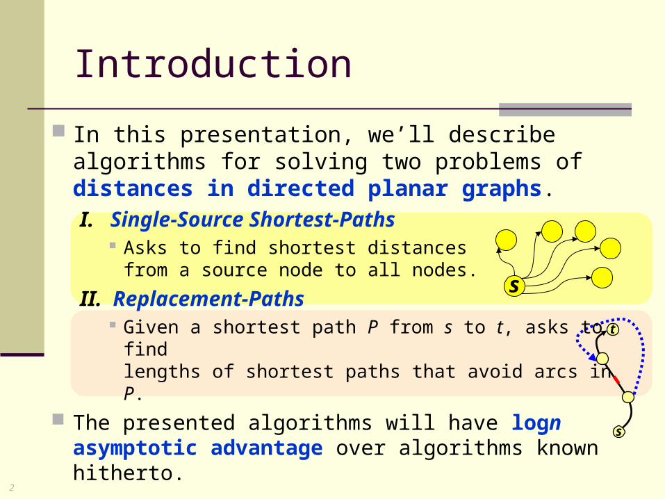
In this presentation, we’ll describe algorithms for solving two problems of distances in directed planar graphs.I. Single-Source Shortest-Paths
Asks to find shortest distancesfrom a source node to all nodes.
II. Replacement-Paths Given a shortest path P from s to t, asks to find
lengths of shortest paths that avoid arcs in P.
The presented algorithms will have lognasymptotic advantage over algorithms known hitherto.

3
Single-Source Shortest-Paths
Part I
s

4
Single-Source Shortest Pathswith Negative Lengths
-0.8
2.7-1
-2
-0.44
1.3-0.5
0.1
1.2
-1.3
-10.01
-0.05
-0.8
2.6
-1
-2 -0.4
1.3
-0.5
0.1
1.2
0.2
-10.70.01
-0.07
-0.75
0.01
-0.8
2.7-1
-2
-0.24
1.3
-0.5
0.1
1.2
-1
0.7
0.01
-0.05
s
-0.8
-0.9
-1
-2
-0.33
1.3
-0.51.2
0.2
-10.70.02
-0.07
-0.75
-1
0.01-0.05
0.21
0.6
0.1
Input
• Directed planar graph G=(V,E), embedded. |V|=n.
• Arc length function len:E.Lengths may be negative.
• No negative cycles.
• Source node s.
Output
• A table dist, such that for each uV, dist(u) is the shortest distance in G from s to u.
-1
9
8

5
Single-Source Shortest Pathswith Negative Lengths
-0.8
2.7-1
-2
-0.44
1.3-0.5
0.1
1.2
-1.3
-10.01
-0.05
-0.8
2.6
-1
-2 -0.4
1.3
-0.5
0.1
1.2
0.2
-10.70.01
-0.07
-0.75
0.01
-0.8
2.7-1
-2
-0.24
1.3
-0.5
0.1
1.2
-1
0.7
0.01
-0.05
s
-0.8
-0.9
-1
-2
-0.33
1.3
-0.51.2
0.2
-10.70.02
-0.07
-0.75
-1
0.01-0.05
0.21
0.6
0.1
-1
9
8
Notes:• We’ll sometimes abbreviate “the shortest distance” as simply “the distance”.• With some abuse of notation, for a path P denote:
e P
len P len e
Input
• Directed planar graph G=(V,E), embedded. |V|=n.
• Arc length function len:E.Lengths may be negative.
• No negative cycles.
• Source node s.
Output
• A table dist, such that for each uV, dist(u) is the shortest distance in G from s to u.

6
In fact, if there are negative cycles, the algorithm can be used to detect them. Run the algorithm, then check if any arc can be
further “relaxed”. That is, check whether there is an arc uv, for
which dist(u)+len(uv)<dist(v). Only if so, declare “G contains a negative cycle”.
Negative Cycles
1.2
0.2
-1
-0.7
-1

7
Progressively Better Bounds
For planar graphs with negative arc lengths.
AlgorithmTimeSpace
Bellman-Ford[1962]
Lipton, Rose, Tarjan[1979]
Heriznger et al.[1997]
Fakcharoenphol and Rao[2006]
Presented Algorithm:Klein, Mozes, Weimanm
[2009]
3/2O n
4/3 2/3log , | |e E
O n D D len e
3logO n n logO n n
2logO n n O n
2O n

8
If Only We Could Run Dijkstra…
Had the arc lengths of G been non-negative, Dijkstra would find dist in O(nlogn) time and O(n) space.
Perhaps we can transform the arc lengths in G to non-negative, so that shortest paths are preserved ?
We could, if we had a feasible price function on the nodes of G, as defined next.

9
Definition: Φ:V is a price function. Φ assigns a real to every node of G.
Φ induces new lengths on the arcs of G: lenΦ(uv) = len(uv) + [Φ(u) - Φ(v)]
lenΦ is called the reduced length with respect to Φ.
If lenΦ(e)0 for all eE, then Φ is called a feasible price function.
Feasible Price Function Φ

10
If We Had a Feasible Price Function Φ…
Consider any u1-to-uk path P in G.
Thus:
1 2 3 1... k kP u u u u u
1 2 1 2
2 3 2 3
1 1
1
...
[ ]
k k k k
k
len u u u u
len u u u u
len u u u u
len P u u
Φlen P
1 2 2 3 1... k klen P len u u len u u len u u

11
Conclusions: A u1-to-uk path P is shortest in G if-and-only-if P is shortest
in GΦ G with reduced arc lengths with respect to Φ.
Since arc lengths in GΦ are non-negative (Φ is feasible),we can run Dijkstra on GΦ, then easily recover the shortest distances in G, as following.
But how can we obtain a feasible price function Φ for G ?
Procedure dijkstra_reduced(G,len,s,Φ) 1. Run Dijkstra on (GΦ,s) with output distΦ. 2. For all tV: Output dist[t]=distΦ[t]-[Φ(s)-Φ(t)].
1[ ]klen P len P u u

12
Example, Φ(v) = r-to-v distance
Let r be an arbitrary node (not necessarily s) of G.For all vV, define Φr(v)shortest r-to-v distance in G.
Observation: Φr(v) is a feasible price function for G. Proof: Denote distr(v) r-to-v distance. Let uvE. So:
Conclusion: to obtain shortest distances from s, we can: 1. Choose any node r in V as we wish.
2. Compute distances in G from r. Set Φr accordingly.
3. Run dijkstra_reduced(G,len,s,Φr).
def.
def.
Length of an -to- path length amongthat ends with all -to- paths
len
r r
r vu v r v
len u v u len u v v
dist u len u v dist v
Shortest
0

13
Overview of the Algorithm
Algorithm Shortet-Paths(G,s):
1. If n2, the problem is trivial ; return the result.
2. Find a separator for G, which cuts it into G0,G1.Let r be an arbitrary node from the separation set.
3. Recursively compute distances d0,d1 from r,in G0 and in G1, respectively.
4. Use d0,d1 to compute distances from r in G.Define Φr accordingly.
5. Run dijkstra_reduced with Φr to obtain the required distances from s in G. Terminate.
s-1.3

14
Algorithm Shortet-Paths(G,s):
1. If n2, the problem is trivial ; return the result.
2. Find a separator for G, which cuts it into G0,G1.
Let r be an arbitrary node from the separation set.
3. Recursively compute distances d0,d1 from r,in G0 and in G1, respectively.
4. Use d0,d1 to compute distances from r in G.Define Φr accordingly.
5. Run dijkstra_reduced with Φr to obtain the required distances from s in G. Terminate.
Overview of the Algorithm
rrG1
G0

15
Algorithm Shortet-Paths(G,s):
1. If n2, the problem is trivial ; return the result.
2. Find a separator for G, which cuts it into G0,G1.Let r be an arbitrary node from the separation set.
3. Recursively compute distances d0,d1 from r,in G0 and in G1, respectively.
4. Use d0,d1 to compute distances from r in G.Define Φr accordingly.
5. Run dijkstra_reduced with Φr to obtain the required distances from s in G. Terminate.
Overview of the Algorithm
G0
G1

16
Overview of the Algorithm
Algorithm Shortet-Paths(G,s):
1. If n2, the problem is trivial ; return the result.
2. Find a separator for G, which cuts it into G0,G1.Let r be an arbitrary node from the separation set.
3. Recursively compute distances d0,d1 from r,in G0 and in G1, respectively.
4. Use d0,d1 to compute distances from r in G.Define Φr accordingly.
5. Run dijkstra_reduced with Φr to obtain the required distances from s in G. Terminate.

17
The Algorithm, Step-by-Step
Steps 1 (trivial case) and 3 (recursion) are self-explanatory.
We’ve already described how to implement step 5 (dijkstra_reduced).
Next, we describe how to implement steps 2 (separator) and 4 (from-r distances in G).
Algorithm Shortet-Paths(G,s)1. Base case: n 2.2. Separation to G0,G1 ; arbitrary rVc.3. Recursion: di Shortest-Paths(Gi ,r).4. Distances from r in G.5. Distances from s in G.

18
Step 2: Separation by a Jordan Curve
-0.8
2.7-1
-2
-0.44
1.3-0.5
0.1
1.2
-1.3
-10.01
-0.05
-0.8
2.6
-1
-2 -0.4
1.3
-0.5
0.1
1.2
0.2
-10.70.01
-0.07
-0.75
0.01
-0.8
2.7-1
-2
-0.24
1.3
-0.5
0.1
1.2
-1
0.7
0.01
-0.05
-0.8
-0.9
-1
-2
-0.33
1.3
-0.51.2
0.2
-10.70.02
-0.07
-0.75
-1
0.01-0.05
0.21
0.6
0.1
• Passes through2S2Sn=O(Sn) nodes, without intersecting any arc.
• Encloses between n/3 and 2n/3 nodes.
• The nodes through which it passes are called boundary nodes.
Denote by Vc the set
of boundary nodes.
-1
9
8

19
Step 2: Jordan Separator – cont.
-0.8
2.7-1
-2
-0.44
1.3-0.5
0.1
1.2
-1.3
-10.01
-0.05
-0.8
2.6
-1
-2 -0.4
1.3
-0.5
0.1
1.2
0.2
-10.70.01
-0.07
-0.75
0.01
-0.8
2.7-1
-2
-0.24
1.3
-0.5
0.1
1.2
-1
0.7
0.01
-0.05
-0.8
-0.9
-1
-2
-0.33
1.3
-0.51.2
0.2
-10.70.02
-0.07
-0.75
-1
0.01-0.05
0.21
0.6
0.1
-1
9
8
• Can be found in O(n) time.• Triangulate the graph with artificial arcs of sufficiently large length, so that shortest distances are not changed, e.g.
• Run Miller’s [1986] algorithm.
1 max | |e E
n len e

20
Sub-graphs G0,G1
-2
-0.44
0.1
1.2
-1.3
-10.01
-0.05
-0.8
2.6
-1
1.3
-0.5
0.1
1.2
0.2
-10.70.01
-0.8
2.7-1
-2
-0.24
1.3
-0.51.2
-1
0.7
0.01
-0.05
-0.8
-0.9
-1
-2
-0.33
1.3
-0.51.2
-1
-0.07
-0.75
-1
-0.05
0.21
0.1
• Obtained by cutting the planar embedding along the Jordan curve and duplicating boundary nodes.
• Denote by G0 and G1 the “external” and “internal” sub-graphs, respectively.
G0, external
0.01
8
r

21
Sub-graphs G0,G1
-0.8
2.7-1
-0.44
1.3-0.5
0.1
-2 -0.4
0.01
-0.07
-0.75
0.01
-0.5
0.1 0.2
-10.70.02
0.01-0.05
0.6
G1, internal
• Obtained by cutting the planar embedding along the Jordan curve and duplicating boundary nodes.
• Denote by G0 and G1 the “external” and “internal” sub-graphs, respectively.
-1
9r
22
Finding distances from r to all nodes in G is done in several stages.
In each stage, we compute some auxiliary tables, which are used by the next stage.
Step 4: From-r Distances in G

23
Finding distances from r to all nodes in G is done in several stages.
In each stage, we compute some auxiliary tables, which are used by the next stage.
Stage 4.1: Boundary-to-Boundary in G0 ,G1
For i=0,1, compute a table i, so that for all pairs of boundary nodes u,v: i[u,v] = u-to-v distance in Gi.
Stage 4.2: r-to-Boundary in GCompute a table B, such that for everyboundary node v: B[v] = r-to-v distance in G.
Stage 4.3: r-to-All in GFor i=0,1, compute a table di’, so that for everynode w of Gi: di’[w] = r-to-w distance in G.Finally, collect the from-r distances in G into table distr.
Step 4: From-r Distances in G

24
Finding distances from r to all nodes in G is done in several stages.
In each stage, we compute some auxiliary tables, which are used by the next stage.
Stage 4.1: Boundary-to-Boundary in G0 ,G1
For i=0,1, compute a table i, so that for all pairs of boundary nodes u,v: i[u,v] = u-to-v distance in Gi.
Stage 4.2: r-to-Boundary in GCompute a table B, such that for everyboundary node v: B[v] = r-to-v distance in G.
Stage 4.3: r-to-All in GFor i=0,1, compute a table di’, so that for everynode w of Gi: di’[w] = r-to-w distance in G.Finally, collect the from-r distances in G into table distr.
Stage 4.1: Boundary-to-Boundary in Gi

25
0.21
Example: Shortest Boundary-to-Boundary in G0
u
-2
-0.44
0.1
1.2
-1.3
-10.01
-0.05
-0.8
2.6
-1
1.3
-0.5
0.1
1.2
0.2
-10.70.01
-0.8
2.7-1
-2
-0.24
1.3
-0.51.2
-1
0.7
0.01
-0.05
v
-0.8
-0.9
-1
-2
-0.33
1.3
-0.51.2
-1
-0.07
-0.75
-1
-0.050.1
0.01
8
2
r

26
-0.8
2.7-1
-0.44
1.3
-0.5
0.1
-2 -0.4
0.01
-0.07
-0.75
0.01
-0.5
0.1 0.2
-10.70.02
0.01-0.05
0.6
-1
9
u
v
Example: Shortest Boundary-to-Boundary in G1
r

27
Stage 4.1: Boundary-to-Boundary in Gi
Via a multiple-source shortest-path algorithm by Klein [K2005], which the article describes briefly. Input:
Output: a table i, so that for every pair of nodes u,v on the face of f, i[u,v]=shortest u-to-v distance in Ĝ.
[K2005] Requires:We provide:
A planar, embedded graph Ĝ with arc lengths in .
Ĝ=Gi, which is a sub-graph of G and so
has all these properties.
A face f of Ĝ.By construction, all boundary nodes in Gi
are on a single face f, which we provide.
Some node u on f, and a table of from-u distances in Ĝ.
Step 3 gave us di = Shortest-Paths(Gi,r).
So u=r and di are just what we need here !

28
Complexity: O(nf2lognf) time and O(nf
2) space,where nf = number of nodes on face of f.
So for nf =|Vc|=O(Sn): O(nlogn) time, O(n) space.
Stage 4.1: Boundary-to-Boundary in Gi
Via a multiple-source shortest-path algorithm by Klein [K2005], which the article describes briefly. Input:
[K2005] Requires:We provide:
A planar, embedded graph Ĝ with arc lengths in .
Ĝ=Gi, which is a sub-graph of G and so
has all these properties.
A face f of Ĝ.By construction, all boundary nodes in Gi
are on a single face f, which we provide.
Some node u on f, and a table of from-u distances in Ĝ.
Step 3 gave us di = Shortest-Paths(Gi,r).
So u=r and di are just what we need here !

29
Finding distances from r to all nodes in G is done in several stages.
In each stage, we compute some auxiliary tables, which are used by the next stage.
Stage 4.1: Boundary-to-Boundary in G0 ,G1
For i=0,1, compute a table i, so that for all pairs of boundary nodes u,v: i[u,v] = u-to-v distance in Gi.
Stage 4.2: r-to-Boundary in GCompute a table B, such that for everyboundary node v: B[v] = r-to-v distance in G.
Stage 4.3: r-to-All in GFor i=0,1, compute a table di’, so that for everynode w of Gi: di’[w] = r-to-w distance in G.Finally, collect the from-r distances in G into table distr.
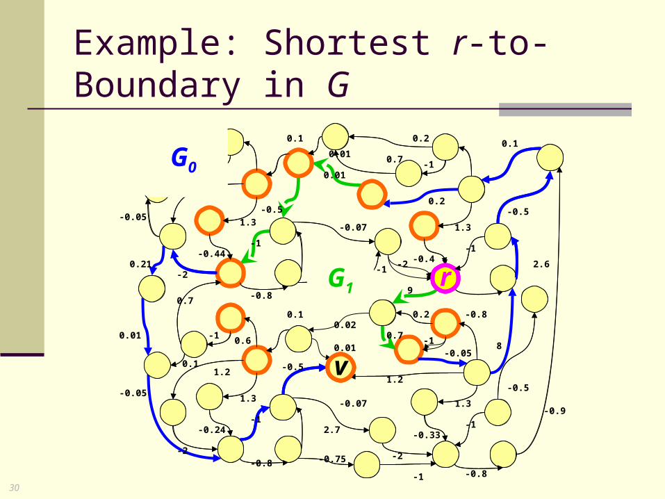
Stage 4.2: r-to-Boundary in G
30
r
v
r
Example: Shortest r-to-Boundary in G
-0.8
2.7-1
-2
-0.44
1.3-0.5
0.1
1.2
-1.3
-10.01
-0.05
-0.8
2.6
-1
-2 -0.4
1.3
-0.5
0.1
0.2
0.2
-10.70.01
-0.07
-0.75
0.01
-0.8
2.7-1
-2
-0.24
1.3
-0.5
0.1
1.2
-1
0.7
0.01
-0.05
-0.8
-0.9
-1
-2
-0.33
1.3
-0.5
8
1.2
0.2
-10.70.02
-0.07
-0.75
-1
0.01-0.05
0.21
0.6
0.1
-1
9
v
G0
G1

31
Every path in G is composed of subpaths that alternate between G1 and G0.
Lemma: let P be a simple r-to-v shortest path in G, where vVc.Then P can be decomposed into at most |Vc| subpaths
so that for each Pj: The endpoints of Pj are boundary nodes. Pj is a (possibly empty) shortest path in Gj mod 2.
Lemma for Stage 4.2: Path Decomposition
0 01
2 4
in
1 3
in i in n
...1 G G GG
P P PP P

32
Lemma for Stage 4.2: Proof
Decompose P into maximal subpaths,each consisting only of nodes in either G0 or G1.
Vc are the only nodes common to both G0,G1, and r,v are in Vc.Thus each subpath Pj starts and ends on a boundary node.
Shortest sub-path property:Pj is a subpath of a shortest path P, thus Pj is shortest in Gj mod 2
(Otherwise, P can be cut short by replacing Pj, a contradiction).
P is simple and so contains at most |Vc| boundary nodes. Hence there are at most |Vc|-1 non-empty subpaths P2P3…. Also, if P begins with an arc of G0, then P1 is empty, r-to-r. Thus P can be decomposed into at most |Vc| subpaths.
r
v

33
The Path Decomposition lemma suggests thatStage 4.2 can be implemented with dynamic programming, whereby P is built iteratively, one optimal subpath at a time.
Stage 4.2: Implementation r
v
0 1
0 0
1 mod 2
| |
Procedure , , , :
1. 0 ; For all :
2. For 1,2,3,...,| |:
2.1 For : min ,
3. c
c
c
c
c
c j j ju V
V
r V
e r v V e v
j V
v V e v e u u v
B e
r_to_boundary

34
Proof of Correctness: Let us prove by induction on j that after table ej
is updated, ej[v]=length of path P that maintains: P is a shortest r-to-v path in G. P can be decomposed into j subpaths P=P1P2…Pj,
where each Pk starts and ends on boundary nodes and is shortest in Gkmod2.
The proof also implies that after the assignment Be|Vc| in step 3, B contains shortest
r-to-boundary distances in G, as required.
Stage 4.2: Correctness
0 1
0 0
1 mod 2
| |
Procedure , , , :
1. 0 ; For all :
2. For 1,2,3,...,| |:
2.1 For : min ,
3. c
c
c
c
c
c j j ju V
V
r V
e r v V e v
j V
v V e v e u u v
B e
r_to_boundary

35
Proof of Correctness – Cont.: Base: j=0, and the claim holds after step 1. Hypothesis: the claim is correct for 1..j-1. Step: Let P from the claim be P=P’Pj, where P’=P1P2…Pj-1
is a shortest r-to-w path in G, for some boundary node w. By the inductive hypothesis, ej-1[w]=len(P’).
Step 2.1 assigns to ej[v] a length, which is at most
ej-1[w]+jmod2[w,v]. So by definition of i, ej[v]len(P).
ej[v] is assigned the length of some path in G, which can
be decomposed into at most j subpaths as defined above. P is a shortest such path, hence ej[v]len(P).
In conclusion, ej[v]=len(P).
Stage 4.2: Correctness
0 1
0 0
1 mod 2
| |
Procedure , , , :
1. 0 ; For all :
2. For 1,2,3,...,| |:
2.1 For : min ,
3. c
c
c
c
c
c j j ju V
V
r V
e r v V e v
j V
v V e v e u u v
B e
r_to_boundary

36
A straightforward implementation would take O(|Vc|3) total time.
We’ll next see an implementation in “almost” O(|Vc|2) total time.
Stage 4.2: Implementation r
v
0 1
0 0
1 mod 2
| |
Procedure , , , :
1. 0 ; For all :
2. For 1, 2,3,...,| |:
2.1 For : min ,
3. c
c
c
c
c
c j j ju V
V
r V
e r v V e v
j V
v V e v e u u v
B e
r_to_boundary

37
An algorithm by Klawe and Kleitman [KK1990]: Input: An x-by-y matrix M, which is “falling staircase”
(defined next). Output: column-minima, i.e. minimum element in
each column of M. Time complexity: O(y(x)+x), where (x) is the inverse
Ackerman function, a very slow-growing function. We’ll show that [KK1990] can be used for
computing every ej[v] via a “Convex Monge” matrix, also defined next.
Stage 4.2: Implementation - cont.

38
To define “falling staircase”, we first need to define “totally monotone”.
Definition: a matrix Mxy is called “totally monotone” when for all i,j:
Stage 4.2: Implementation - cont.
' ' ' 'If then also ' , ' :ij ij i j i jM M i i j j M M
j j'
i
i'
'j j
i

39
Definition: a matrix Mxy is called “falling staircase” when: It has the following form.
Every four indices of non-blank elements in it maintain the “total monotonicity” property.
Stage 4.2: Implementation - cont.
' ' ' 'If then also ' , ' :ij ij i j i jM M i i j j M M
'
j j'
i
i
M(1,1) mustnot be blank.
“Blanks”

40
We now define a property stronger than “totally monotocity”. Definition: a matrix Mxy is called “Convex Monge” when:
Stage 4.2: Implementation - cont.
j j'
i
i'
' ' ' '' , ' : ij i j ij i ji i j j M M M M

41
Convex Monge:
Properties of Convex Monge: M is Convex Monge M is Totally Monotone.
Proof:
Convex Monge is preserved under:1) Transpose. 2) Order reversal of both rows and columns.
Proof:
1) 2)
Stage 4.2: Implementation - cont.
j j'
i
i'
' ' ' '' , ' : ij i j ij i ji i j j M M M M
' ' ' '
' ' ' '
Not Totally Monontone and
Not Convex Monge
ij ij i j i j
ij i j ij i j
M M M M
M M M M
Transpose
...1 ... 2... ...1 ... 3...
...3 ... 4... ...2 ... 4...
order reversal
...1 ... 2... ...4 ... 3...
...3 ... 4... ...2 ... 1...

42
Suppose we are in interation #j. For every v in Vc, we wish to compute:
Consider the |Vc|-by-|Vc| matrix A defined as:
Thus for any v in Vc, computing ej[vl] isequivalent to finding the minimum of column Al.
It remains to show that the lower triangle of A is a falling staircase, as is A’s upper triangle after O(1) manipulations.
Thereafter, we obtain column-minima in A by running [KK1990] on each triangle and combining the results.
Stage 4.2: [KK1990]
1 mod 2 ,kl j k j k lA e v v v
1 mod 2min ,c
j j ju V
e v e u u v
1
32
4…
C
C
1 2 … … V
1
2
V
l
k

43
Stage 4.2: [KK1990]
Lemma 4.4: for any four indices kk’ll’ as illustrated, that is are all in A’s upper triangle,the Convex Monge property holds:
1 mod 2 ,kl j k j k lA e v v v
' ' ' 'kl k l k l klA A A A
k
k'
l l'' ' ' ', , ,kl kl k l k lA A A A

44
Stage 4.2: [KK1990]
Lemma 4.4: for any four indices kk’ll’ as illustrated, that is are all in A’s upper triangle,the Convex Monge property holds:
Proof: without loss of generality, assume j mod 2 = 1, so
this iteration uses 1, that of the internal subgraph. By the way boundary nodes are numbered,
k,k’,l,l’ are ordered as illustrated: Consider two shortest paths:
k-to-l and k’-to-l’. These pathsintersect.
1 mod 2 ,kl j k j k lA e v v v
' ' ' 'kl k l k l klA A A A
k
k'
l l'' ' ' ', , ,kl kl k l k lA A A A
l’
l k… k’

45
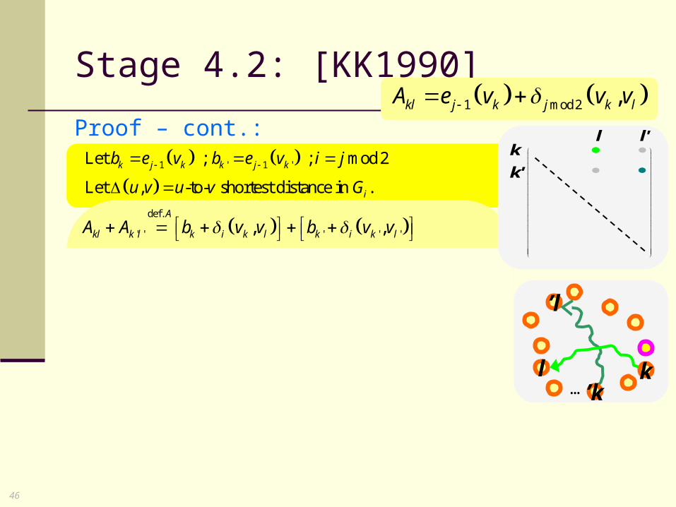
Stage 4.2: [KK1990]
Lemma 4.4: for any four indices kk’ll’ as illustrated, that is are all in A’s upper triangle,the Convex Monge property holds:
Proof – cont.: Due to planarity, the intersection occurs at some
node w. We can therefore dissect the paths at w
into four sub-paths as shown. By the shortest sub-path property,
the illustrated k-to-w, k’-to-w, w-to-land w-to-l’ are shortest in Gjmod2.
1 mod 2 ,kl j k j k lA e v v v
' ' ' 'kl k l k l klA A A A
k
k'
l l'' ' ' ', , ,kl kl k l k lA A A A
l’
l kk’…
w
46
def.
' ' ' ' '
shortestsub-paths
' ' '
rearrange
' ' '
def.
' ' '
, ,
, , , ,
, , , ,
, ,
A
kl k l k i k l k i k l
k k l k k l
k k l k k l
k k l k k l
A A b v v b v v
b v w w v b v w w v
b v w w v b v w w v
b v v b v v
in def.
' ' ' ' ' , ,cV A
k i k l k i k l kl k lb v v b v v A A
Stage 4.2: [KK1990]
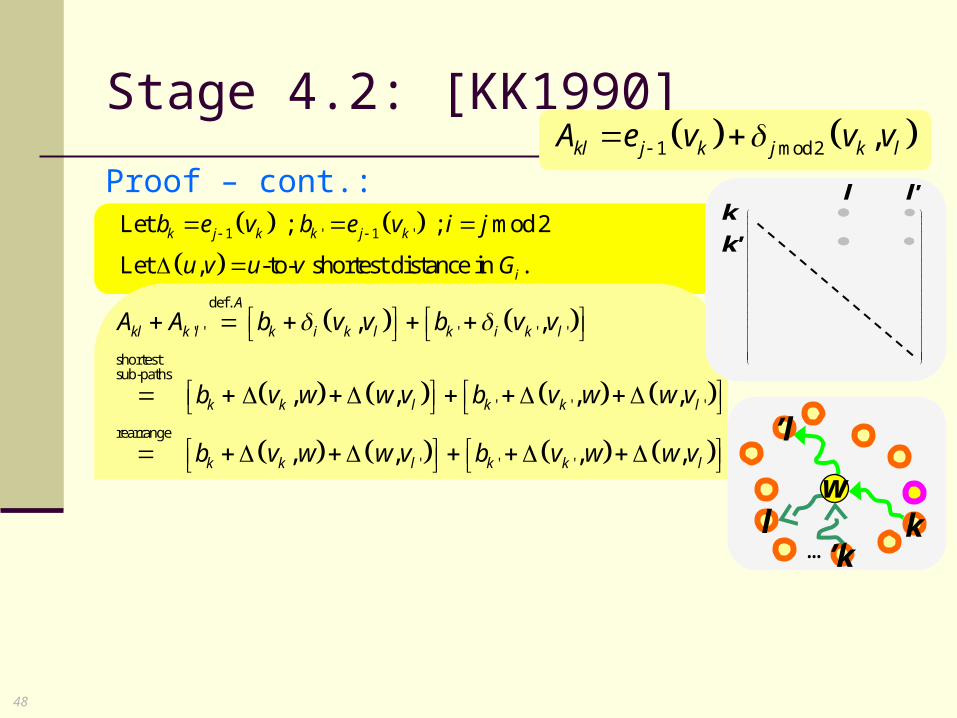
Proof – cont.: 1 mod 2 ,kl j k j k lA e v v v
1 ' 1 'Let ; ; mod 2
Let , -to- shortest distance in .
k j k k j k
i
b e v b e v i j
u v u v G
l’
l k… k’
l l'k
k'

47
def.
' ' ' ' '
shortestsub-paths
' ' '
rearrange
' ' '
def.
' ' '
, ,
, , , ,
, , , ,
, ,
A
kl k l k i k l k i k l
k k l k k l
k k l k k l
k k l k k l
A A b v v b v v
b v w w v b v w w v
b v w w v b v w w v
b v v b v v
in def.
' ' ' ' ' , ,cV A
k i k l k i k l kl k lb v v b v v A A
Stage 4.2: [KK1990]
Proof – cont.: 1 mod 2 ,kl j k j k lA e v v v
1 ' 1 'Let ; ; mod 2
Let , -to- shortest distance in .
k j k k j k
i
b e v b e v i j
u v u v G
l’
l kk’…
w
l l'k
k'
48
def.
' ' ' ' '
shortestsub-paths
' ' '
rearrange
' ' '
def.
' ' '
, ,
, , , ,
, , , ,
, ,
A
kl k l k i k l k i k l
k k l k k l
k k l k k l
k k l k k l
A A b v v b v v
b v w w v b v w w v
b v w w v b v w w v
b v v b v v
in def.
' ' ' ' ' , ,cV A
k i k l k i k l kl k lb v v b v v A A
Stage 4.2: [KK1990]
Proof – cont.: 1 mod 2 ,kl j k j k lA e v v v
1 ' 1 'Let ; ; mod 2
Let , -to- shortest distance in .
k j k k j k
i
b e v b e v i j
u v u v G
l kk’…
w
l’
l l'k
k'

49
def.
' ' ' ' '
shortestsub-paths
' ' '
rearrange
' ' '
def.
' ' '
, ,
, , , ,
, , , ,
, ,
A
kl k l k i k l k i k l
k k l k k l
k k l k k l
k k l k k l
A A b v v b v v
b v w w v b v w w v
b v w w v b v w w v
b v v b v v
in def.
' ' ' ' ' , ,cV A
k i k l k i k l kl k lb v v b v v A A
Stage 4.2: [KK1990]
Proof – cont.: 1 mod 2 ,kl j k j k lA e v v v
1 ' 1 'Let ; ; mod 2
Let , -to- shortest distance in .
k j k k j k
i
b e v b e v i j
u v u v G
l kk’…
w
l l'k
k'
l’

50
Stage 4.2: [KK1990] 1 mod 2 ,kl j k j k lA e v v v
Proof – cont.:
1 ' 1 'Let ; ; mod 2
Let , -to- shortest distance in .
k j k k j k
i
b e v b e v i j
u v u v G
def.
' ' ' ' '
shortestsub-paths
' ' '
rearrange
' ' '
def.
' ' '
, ,
, , , ,
, , , ,
, ,
A
kl k l k i k l k i k l
k k l k k l
k k l k k l
k k l k k l
A A b v v b v v
b v w w v b v w w v
b v w w v b v w w v
b v v b v v
in def.
' ' ' ' ' , ,cV A
k i k l k i k l kl k lb v v b v v A A
l’
l kk’…
l l'k
k'

51
Proof – cont.:
The proof for the lower triangle of A is symmetric. To turn the upper triangle of A into falling staircase,
reverse the order of both its rows and columns in O(1).
Stage 4.2: [KK1990] 1 mod 2 ,kl j k j k lA e v v v
1 ' 1 'Let ; ; mod 2
Let , -to- shortest distance in .
k j k k j k
i
b e v b e v i j
u v u v G
def.
' ' ' ' '
shortestsub-paths
' ' '
rearrange
' ' '
def.
' ' '
, ,
, , , ,
, , , ,
, ,
A
kl k l k i k l k i k l
k k l k k l
k k l k k l
k k l k k l
A A b v v b v v
b v w w v b v w w v
b v w w v b v w w v
b v v b v v
in def.
' ' ' ' ' , ,cV A
k i k l k i k l kl k lb v v b v v A A
l’
l kk’…
l l'k
k'

52
Stage 4.2: Summary
0 1
0 0
1 mod 2
| |
Procedure , , , :
1. 0 ; For all :
2. For 1, 2,3,...,| |:
2.1 For : min ,
3. c
c
c
c
c
c j j ju V
V
r V
e r v V e v
j V
v V e v e u u v
B e
r_to_boundary
1 mod 2 ,kl j k j k lA e v v v
ComparingKK1990
( 2 ( ) ) ( )C C C C CO V V V O V V
2( ) ( )C CO V V O n n
Step 2.1 is implemented via [KK1990], which requires access to matrix A, defined as Note: We don’t actually compute A. Instead, whenever
[KK1990] asks for some Akl, we compute Akl in O(1).
We run [KK1990] on each triangle of A, then compare the results to derive A’s column-minima. So step 2.1 is performed in total time:
Step 2 performs |Vc| iterations.
Since |Vc|=O(Sn), the total time complexity of stage 4.2 is:

53
Finding distances from r to all nodes in G is done in several stages.
In each stage, we compute some auxiliary tables, which are used by the next stage.
Stage 4.1: Boundary-to-Boundary in G0 ,G1
For i=0,1, compute a table i, so that for all pairs of boundary nodes u,v: i[u,v] = u-to-v distance in Gi.
Stage 4.2: r-to-Boundary in GCompute a table B, such that for everyboundary node v: B[v] = r-to-v distance in G.
Stage 4.3: r-to-All in GFor i=0,1, compute a table di’, so that for everynode w of Gi: di’[w] = r-to-w distance in G.Finally, collect the from-r distances in G into table distr.
Stage 4.3: r-to-All in G

54
r
v
r
Example: Shortest r-to-v in G, v G0
u
v
-0.8
2.7-1
-2
-0.44
1.3-0.5
0.1
1.2
-1.3
-10.01
-0.05
-0.8
2.6
-1
-2 -0.4
1.3
-0.5
0.1
0.2
0.2
-10.70.01
-0.07
-0.75
0.01
-0.8
2.7-1
-2
-0.24
1.3
-0.5
0.1
1.2
-1
0.7
0.01
-0.05
-0.8
-0.9
-1
-2
-0.33
1.3
-0.5
8
1.2
0.2
-10.70.02
-0.07
-0.75
-1
0.01-0.05
0.21
0.6
0.1
-1
9
G0
G1

55
Stage 4.3: Observation
Consider a shortest r-to-v path P in G, for any vGi.
Denote by u the last boundary node that P visits (possibly u=r or u=v).
Observation: P=P1P2, where Pj is possibly empty, and by the shortest sub-path property:
P1 is a shortest r-to-u path.
And we know len(P1)=B[u].
P2 is a shortest u-to-v path,entirely in Gi.
u
v
r

56
Construct a graph G’i from Gi as following. Remove all arcs entering r.
Stage 4.3: Construction Gi ’
rG’0:

57
Construct a graph G’i from Gi as following. Remove all arcs entering r. For each boundary node u,
add a new arc ru with length B[u].
Stage 4.3: Construction Gi ’
rG’0:

58
Lemma 5.2: for each node v of G’i,
r-to-v distance in G’i = r-to-v distance in G !
Stage 4.3: Lemma
u
v
r

59
Lemma 5.2: same from-r distances in G’i as in G.
Proof: : distances in G’i are no shorter than in G, since each
arc of G’i corresponds to some path in G.
: Take a shortest r-to-v path P in G. Let P1,P2,u be as in the decomposition of P in the observation. Therefore:
len(P1)=B[u]=len(e’), where e’=new ru.
Every arc e in P2 is in Gi and does not enter r, thus e is also in G’i, and P2 is a path in G’i.
So P’=e’P2 is some r-to-v path in G’i, and len(P’)=len(P).
Stage 4.3: Lemma

60
So by lemma 5.2, we can find the desired from-r distances in G by finding them in G’i, using dijkstra_reduced.
To this end, we need i, a feasible price function for G’i, which we define next.
Stage 4.3: i

61
Recall that recursive step 3 captured in table di the shortest from-r distances in Gi.
Lemma 5.3: let .Then the following is a feasible price function for G’i.
maxC
i iu V
p d u B u
Stage 4.3: i
i
ii
p v rv
d v otherwise

62
Recall that recursive step 3 captured in table di the shortest from-r distances in Gi.
Lemma 5.3: let .Then the following is a feasible price function for G’i.
Proof: let e=wt be an arc of G’i. By definition, . Note that pi0, by definition of di and B.
If e appears also in Gi, then tr, and:
maxC
i iu V
p d u B u
Stage 4.3: i
i
ii
p v rv
d v otherwise
def. def.
def. p 0,def.
If : 0
Otherwise: 0
i i
i
i i i
i
d
i i
d
i i
w r len e d w len e d t
len e len e p d t
i i ilen e len e w t
63
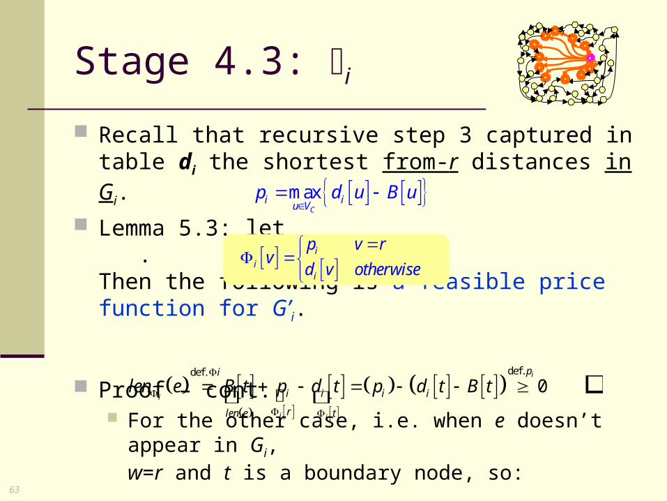
Recall that recursive step 3 captured in table di the shortest from-r distances in Gi.
Lemma 5.3: let .Then the following is a feasible price function for G’i.
Proof – cont. For the other case, i.e. when e doesn’t appear in Gi,
w=r and t is a boundary node, so:
maxC
i iu V
p d u B u
Stage 4.3: i
i
ii
p v rv
d v otherwise
def. def.
0i
i
i i
pi
i i i i
rlen e t
len e B t p d t p d t B t

64
We can now join all these steps to form an implementation of stage 4.3.
Finally, we combine tables d’0 and d’1 to obtainfrom-r distances in G, as following.
Complexity of stage 4.3: O(nlogn) time, O(n) space.
Stage 4.3: Implementation
For 0,1:
1. Construct ' from as described earlier.
2. Define the feasible a price function for ' .
3. .
i i
i i
i
G G
G
i iiCompute = dijkstra_reduced G' ,len,r,Φd'
0 0r
1
d' v v Gdist v =
d' v otherwise
1.
2.
3. log
Time Complexity
O n
O n
O n n

65
Output: distance from r to each node of G. O(nlogn) time, O(n) space.
Stage 4.1: Boundary-to-Boundary in G0 ,G1 By [K2005]. O(nlogn) time, O(n) space.Output: for all u,vVc, i[u,v] = u-to-v distance in Gi.
Stage 4.2: r-to-Boundary in GBy DP and [KK1990]. O(n(n)) time, O(n) space.Output: for all uVc, B[u] = r-to-u distance in G.
Stage 4.3: r-to-All in GBy construction of G’i. O(nlogn) time, O(n) space.Output: for all v in V, distr[v]= r-to-v distance in G.
Step 4: Summary
66
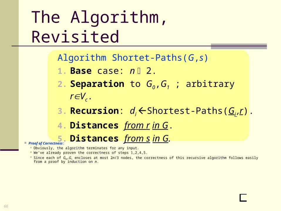
The Algorithm, Revisited
Algorithm Shortet-Paths(G,s)
1. Base case: n 2.
2. Separation to G0,G1 ; arbitrary rVc.
3. Recursion: di Shortest-Paths(Gi ,r).
4. Distances from r in G.
5. Distances from s in G. Proof of Correctness:
Obviously, the algorithm terminates for any input. We’ve already proven the correctness of steps 1,2,4,5. Since each of G0,G1 encloses at most 2n/3 nodes, the correctness of this recursive algorithm follows easily
from a proof by induction on n.

67
We shall next prove the complexity of the algorithm: O(nlog2n) time, O(n) space.
Time Complexity: Step 1 takes O(1) time. Step 2 takes O(n) time. Steps
4,5 take O(nlogn) time. So denoting by n0,n1 the number of nodes in G0,G1,
respectively, the following recursive formula describes the total time complexity.
Proof of Complexity
0 1
Step 3 All other steps
logT n T n T n O n n
Algorithm Shortet-Paths(G,s)1. Base case: n 2.2. Separation to G0, G1 ; arbitrary rVC.3. Recursion: di Shortest-Paths(Gi ,r).4. Distances from r in G.5. Distances from s in G.

68
Lemma 6.1: Because and , . Intuitively, this holds because recursion depth is O(logn).
Following is the proof as it appears in the article draft. In fact, since G0,G1 also include up to boundary
nodes, and However, for it holds that So in the proof, you can replace 2/3 with 4/5 and
with , and the proof still holds. Proof:
Explicitly, we wish to show there are constants K,C > 0, so that for all
We do so by induction on n.
Time Complexity 0 1 logT n T n T n O n n
0 1
2,
3
nn n 0 1 4n n n n n
2logT n O n n
2: log .n T n n n K C
0 1, 2 / 3 2 2n n n n 0 1 4 2 .n n n n 2 2 n
450,n 2 / 3 2 2 .n n 4 / 5n
4n n 4 2n n

69
Lemma 6.1: Because and , .
Proof – Cont.: Base: For reasons we specify later, fix K so that
for all n>K:
Now, for all Let C0 be such that
Let C1 satisfy the big-O in the recursive formula
Thus we can fix C as
Time Complexity 0 1 logT n T n T n O n n
0 1
2,
3
nn n 0 1 4n n n n n
2logT n O n n
K n 3K :
20 logT n C n n
0 1 1 logT n T n T n C n n
10
CC = max C ,
log 3 / 2
2 log 3 / 21 2
log log 42 log 3 / 2 2
n n n n n n
K

70
Time Complexity 0 1 logT n T n T n O n n
0 1
2,
3
nn n 0 1 4n n n n n
2logT n O n n
3 'K n n
0 1
0 1
0 1
InductionHypothesis
2 20 0 1 1 1
,2 /3
20 1 1
4 2
1
log
log log log
log 2 / 3 log
4 log 2 / 3 log log
n nn
n nn n
T n T n T n O n n
Cn n Cn n C n n
C n n n C n n
C n n n C n n
0 1,3
nn n K
Lemma 6.1: Because and , .
Proof – Cont.: Hypothesis: the claim holds for all .
Step: Take n=n’. Since :

71
Lemma 6.1: Because and , .
Proof – Cont.: Step – Cont.: Expanding , we obtain:
So it suffices to show that (~)0, or equivalently that:
Indeed, this holds, by the choice of C and K.
Time Complexity 2
14 log 2 / 3 log logT n C n n n C n n
0 1
2,
3
nn n 0 1 4n n n n n
2logT n O n n
2
2
21
2
2
21
4 loglog
4 log 2 / 3 log
4 log log
4 log 2 / 3 log
C n nT n Cn n
C n n C n
C n nCn n
C n n C n
~
- 2C n + 4 n log 3 / 2 logn
- 2C nlog 3 / 2 logn
2log 2 / 3 log n
21
12
log 3 / 221 log log 4
2 log 3 / 2 log 3 / 2 2
Cn n n n n n
C
1At most log , by choice of At least , by choice of 2
n n KC

72
We now turn for the space bound. Due to steps 1,2,4,5, one invocation takes O(n) space.
That is, there are constants C,K such that for all nK,one invocation takes at most Cn time.
So for all nK, the total space complexity is given by
Thus the algorithm has O(n) space complexity.
Space Complexity
0 1
GeometricSeries
max ,
2 4 13
3 9 1 2 / 3
S n O n S n S n
n nCn C C C n Cn O n
Algorithm Shortet-Paths(G,s)1. Base case: n 2.2. Separation to G0,G1 ; arbitrary rVc.3. Recursion: di Shortest-Paths(Gi ,r).4. Distances from r in G.5. Distances from s in G.

73
In conclusion, algorithm Shortest-Paths(G,s):
Solves single-source shortest paths ina planar graph G with negative arc lengths.
Runs in O(nlog2n) time and O(n) space.
Wrap Up Algorithm Shortet-Paths(G,s) Base case: n 2. Separation to G0,G1 ; arbitrary rVc. Recursion: di Shortest-Paths(Gi ,r). Distances from r in G. Distances from s in G.

74
Replacement-Paths
Part II
s
t
75
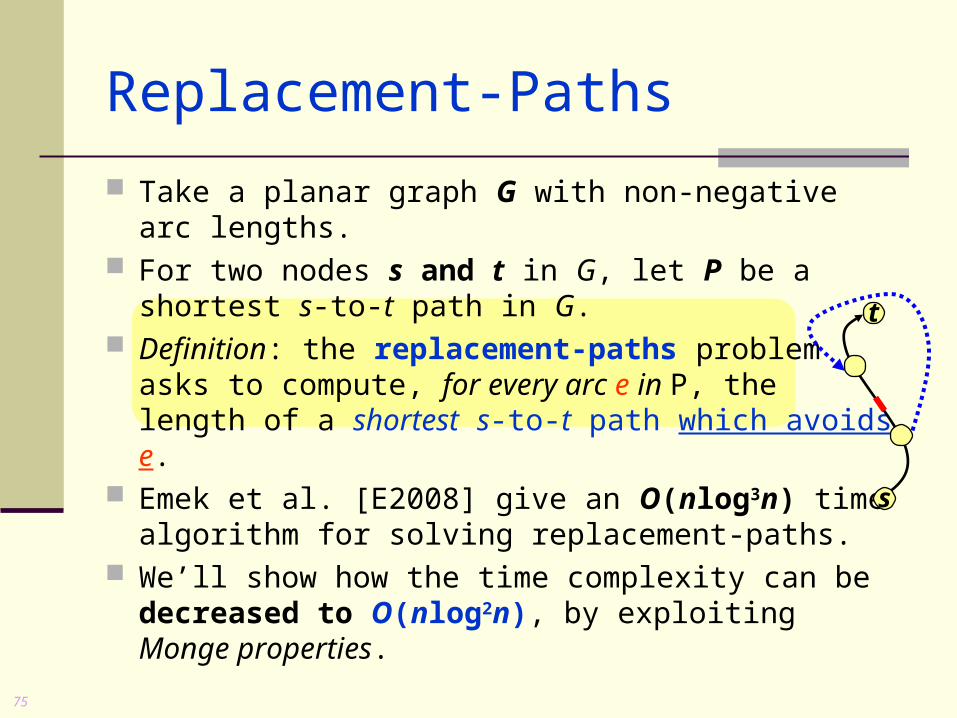
Replacement-Paths
Take a planar graph G with non-negative arc lengths. For two nodes s and t in G, let P be a shortest s-to-t
path in G. Definition: the replacement-paths problem
asks to compute, for every arc e in P, thelength of a shortest s-to-t path which avoids e.
Emek et al. [E2008] give an O(nlog3n) timealgorithm for solving replacement-paths.
We’ll show how the time complexity can be decreased to O(nlog2n), by exploiting Monge properties.
s
t

76
Replacement-Paths
Let , where . Consider a replacement-path Q
which avoids a specific edge e in P. Q can be decomposed
as Q=Q1Q2Q3, so that: Q1 is a (maybe empty) prefix of P.
Q2 is a shortest ui-to-uj+1 paththat avoids any other node in P.
Q3 is a (maybe empty) suffix of P.
1 2 1, ,..., pP u u u 1 1, pu s u t
s
t
i
j+1
Q1
Q2
Q3
e

77
Let , where . Replacement-path Q=Q1Q2Q3.
Q2 leaves P either “from the Left” or “from the Right”,and similarly meets back with P, but doesn’t cross P. Call D{LL,RR,LR,RL} the “orientation” of Q2.
Replacement-Paths
1 2 1, ,..., pP u u u 1 1, pu s u t
s
t
i
j+1
s
t
i
j+1
s
t
i
j+1
s
t
i
j+1
LL
RR
LR
RL

78
Our goal is to compute len(Q), but we don’t know i,j,D. Denote by the shortest x-to-y distance in G. Consider any specific i,j.
can be computed from P in O(p) time. can be computed from P in O(p) time.
Thus we can preprocess and store in O(p) timethe values of len(Q1) and len(Q3) for all i,j=1..p.
Replacement-Paths 1 1 1
, orientation
,..., ,..., ,...,i j p
s t
Q u u u u 2Q D
1 G ilen Q = δ s,u
3 1G jlen Q = δ u ,t
Gδ x, y

79
Replacement-Paths 1 1 1
, orientation
,..., ,..., ,...,i j p
s t
Q u u u u 2Q D
1 G ilen Q = δ s,u
3 1G jlen Q = δ u ,t
PAD - query2 G,Dlen Q = i, j
Gδ x, y
Our goal is to compute len(Q), but we don’t know i,j,D. Denote by the shortest x-to-y distance in G. Consider any specific i,j.
can be computed from P in O(p) time. can be computed from P in O(p) time.
Thus we can preprocess and store in O(p) timethe values of len(Q1) and len(Q3) for all i,j=1..p.
For Q2, from ui to uj+1 with orientation D, [E2008] defines
where PAD-query is computed in O(logn) time via some special data structure.

80
Our goal is to compute len(Q), but we don’t know i,j,D. [E2008] further defines four p-by-p matrices lenD.
So for any specific i,j,D:
Thus any entry can be computed in O(logn) time.
Replacement-Paths 1 1 1
, orientation
,..., ,..., ,...,i j p
s t
Q u u u u 2Q D
1 2 3
For , , , and 1 , :
where is as defined above, is -to- with orientation .
D LL RR RL LR i j p
Q Q Q Q u u
D
2 i j+1
len i, j = len Q
Q D
Dlen i, j
, 1, PAD-query , ,G i G D G j= s u i j u t
1 2 3len Q len Q
D
len Q
len i, j

81
Observation: Suppose that Q needs to avoid arc ek=uk uk+1, k[1..p].
Then Q2 begins at some ui and ends at some uj+1, so that i[1..k] and j[k..p].
Denote by range(k) this range of rows i and columns j.
Thus finding len(Q) is equivalent to finding theminimum element in portion range(k) of lenD,among all four D=LL,RR,LR,RL.
Replacement-Paths 1 1 1
, orientation
,..., ,..., ,...,i j p
s t
Q u u u u 2Q D

82
The O(nlog3n) time complexity of [E2008] arises from recursive calls to procedure District, defined as: Input: Output:
Procedure District
1 and , , , .a b p D LL RR LR RL
row-minima column-minima
..
and in portion
of , where /. 2 ., . Da av len avg ag a g b bv
1 ... ... ...
12
pavg
avg
p
b
a

83
Initially, District(1,p) is called, that is a=1 and b=p. Thus it effectively computes the minimum of
range(p/2) = [1..p/2 , p/2.. p].
Procedure District
1 2 . . . . . . / 2
2
1
/
2
p p
p
p

84
Initially, District(1,p) is called, that is a=1 and b=p. Thus it effectively computes the minimum of
range(p/2) = [1..p/2 , p/2.. p]. Then, District is called recursively as
Procedure District
1 2 . . . . . . / 2
2
1
/
2
p p
p
p
and DDistri istricct a, t avgavg - 1 + 1,b

85
1 2 . . . . . . / 2
2
1
/
2
p p
p
p
Procedure District
Observation: Combining the results of District(a,b) and District(a,avg-1)
yields the minimum of range(p/4) = [1..p/4 , p/4..p]. Combining the results of District(a,b) and District(avg+1,b)
yields the minimum of range(3p/4) = [1..3p/4 , 3p/4..p].

86
District(1,p) computes the minimum of all range(k), k=1..p.
Procedure District
Observation: Combining the results of District(a,b) and District(a,avg-1)
yields the minimum of range(p/4) = [1..p/4 , p/4..p]. Combining the results of District(a,b) and District(avg+1,b)
yields the minimum of range(3p/4) = [1..3p/4 , 3p/4..p]. The recursion stops when b–a1.
Thus District(1,p) has recursion depth O(logp). So in conclusion:

87
[E2008] shows that District(a,b) can be computed in time
The log2 is due to usage of divide-and-conquer for computing minima in each of the rectangular portions.
Since p=O(n), the total time complexity of District(1,p) is
Procedure District – Running Time
O n nlog3
logO b a n 2log b - a

88
[E2008] shows that District(a,b) can be computed in time
The log2 is due to usage of divide-and-conquer for computing minima in each of the rectangular portions.
Since p=O(n), the total time complexity of District(1,p) is
Let us show that each of the rectangular portions has a Monge property. This allows finding minima more quickly than divide-and-
conquer. Consequently, the running time will decrease to:
Procedure District – Running Time
( , ) log
(1, )
T District a b O b a n
T District p O n
2
log b - a
log n
O n nlog3
logO b a n 2log b - a

89
Monge Property of lenD
Lemma 7.1: the upper triangle of lenD is eitherConvex Monge or Concave Monge.
We care only about the upper triangle because Q2 is a ui-to-uj+1 path such that ij.
i
i'
j j'
Convex Monge Concave Monge
' ' ' 'ij i j i j ijA A A A
i
i'
j j'
' ' ' 'ij i j i j ijA A A A

90
Monge Property of lenD
Lemma 7.1: the upper triangle of lenD is eitherConvex Monge or Concave Monge.
Proof: Recall that .
It suffices to prove for the upper triangle of PAD-query. That is because adding to all elements in row i and
to all elements in column j preserves the property.
1 2 3
1, ,G i G
len Q len Q len Q
js u u t= PAD - query D G,Dlen i, j i, j
,G is u
Convex Monge Concave Monge
1,G ju t
i
i'
j j'i
i'
j j'

91
Monge Property of lenD
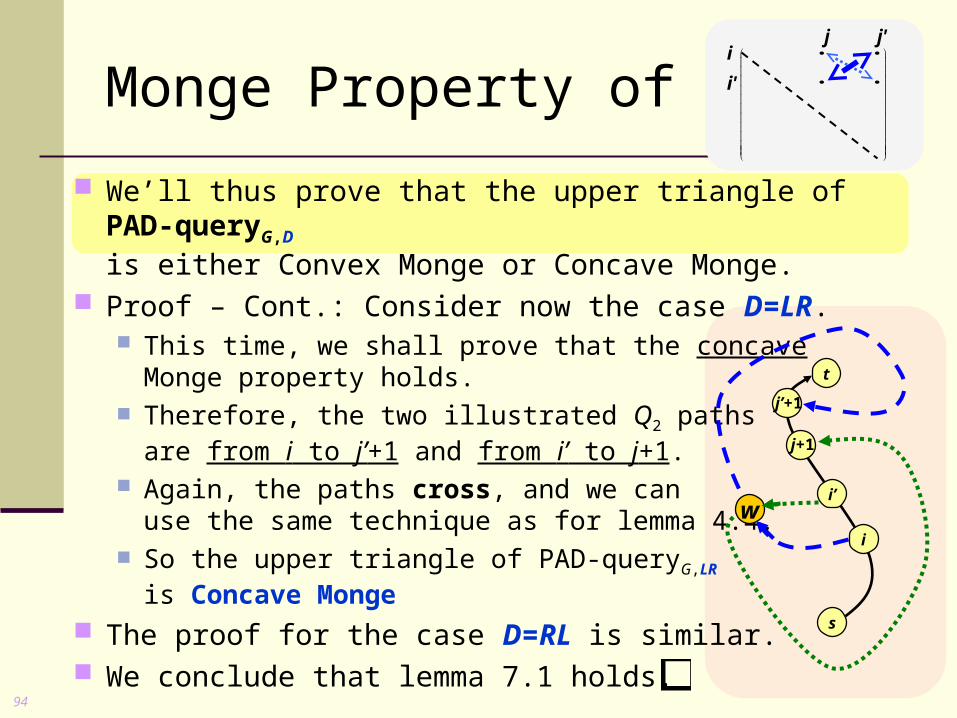
We’ll thus prove that the upper triangle of PAD-queryG,D
is either Convex Monge or Concave Monge. Proof: Consider first the case D=LL.
Illustrated are two Q2 paths with orientation D,one from i to j, the other from i’ to j’.
Since i<i’j<j’ (in the upper triangle),the nodes are ordered as shown.
i
i'
j j'
t
i
j+1
i’
j’+1
s

92
Monge Property of lenD
We’ll thus prove that the upper triangle of PAD-queryG,D
is either Convex Monge or Concave Monge. Proof: Consider first the case D=LL.
Illustrated are two Q2 paths with orientation D,one from i to j, the other from i’ to j’.
Since i<i’j<j’ (in the upper triangle),the nodes are ordered as shown.
Therefore, the two Q2 paths must crossat some node w.
Following the same logic as in the proofof lemma 4.4, we obtain that the uppertriangle of PAD-queryG,LL is Convex Monge.
The proof for the case D=RR is similar.
i
i'
j j'
t
i
j+1
i’
j’+1
s
w

93
Monge Property of lenD
We’ll thus prove that the upper triangle of PAD-queryG,D
is either Convex Monge or Concave Monge. Proof – Cont.: Consider now the case D=LR.
This time, we shall prove that the concaveMonge property holds.
Therefore, the two illustrated Q2 pathsare from i to j’+1 and from i’ to j+1.
i
i'
j j'
t
i
j+1
i’
j’+1
s
94
Monge Property of lenD
We’ll thus prove that the upper triangle of PAD-queryG,D
is either Convex Monge or Concave Monge. Proof – Cont.: Consider now the case D=LR.
This time, we shall prove that the concaveMonge property holds.
Therefore, the two illustrated Q2 pathsare from i to j’+1 and from i’ to j+1.
Again, the paths cross, and we canuse the same technique as for lemma 4.4.
So the upper triangle of PAD-queryG,LR
is Concave Monge The proof for the case D=RL is similar. We conclude that lemma 7.1 holds.
i
i'
j j'
w
t
i
j+1
i’
j’+1
s

95
We’ll now show how the Monge property can be exploited to decrease the time it takes to find minima.
Algorithm SMAWK [Aggrawal et al., 1987]. Input: An x-by-y, totally monotone matrix M. Output: All row-maxima of M. Running time: O(x + y) !
SMAWK, row-maxima

96
Recall that Convex Monge Totally Monotone. So if we take a Convex Monge matrix M:
Transpose M (Monge preservered), then run SMAWK to obtain column-maxima of M.
SMAWK, Minima and Maxima
Transpose
...1 ... 2... ...1 ... 3...
'
...3 ... 4... ...2 ... 4...
M M
Columns of are now
raws of '.
M
M

97
Recall that Convex Monge Totally Monotone. So if we take a Convex Monge matrix M:
Transpose M (Monge preservered), then run SMAWK to obtain column-maxima of M.
We can obtain all row-minima of M from SMAWK: Multiply M by -1 and reverse order of columns, in O(1).
Run SMAWK on M’, multiply the output by -1.
SMAWK, Minima and Maxima
...1 ... 2... ... 2 ... 1...
'
...3 ... 4... ... 4 ... 3...
M M
, ,
' is Convex Monge, and
max ' minj jjj
M
M
M i i
Transpose
...1 ... 2... ...1 ... 3...
'
...3 ... 4... ...2 ... 4...
M M
Columns of are now
raws of '.
M
M

98
Recall that Convex Monge Totally Monotone. So if we take a Convex Monge matrix M:
Transpose M (Monge preservered), then run SMAWK to obtain column-maxima of M.
We can obtain all row-minima of M from SMAWK: Multiply M by -1 and reverse order of columns, in O(1).
Run SMAWK on M’, multiply the output by -1. We can obtain all column-minima of M from SMAWK:
Transpose M (Monge preserved) then use row-minima trick.
SMAWK, Minima and Maxima
...1 ... 2... ... 2 ... 1...
'
...3 ... 4... ... 4 ... 3...
M M
, ,
' is Convex Monge, and
max ' minj jjj
M
M
M i i
Transpose
...1 ... 2... ...1 ... 3...
'
...3 ... 4... ...2 ... 4...
M M
Columns of are now
raws of '.
M
M

99
Decreasing Time of District
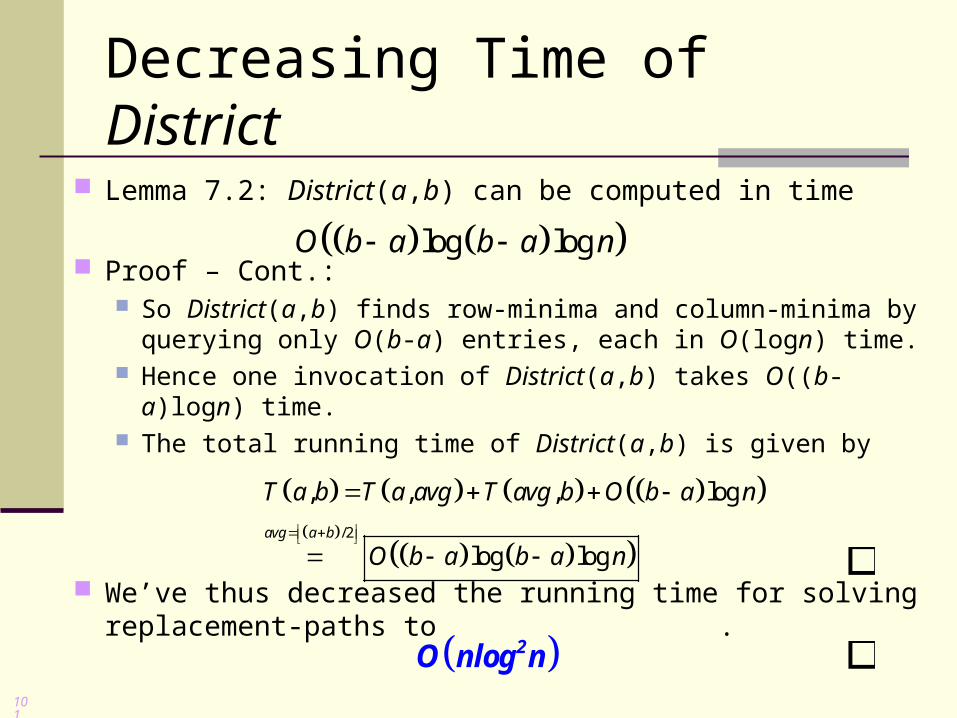
Lemma 7.2: District(a,b) can be computed in time
Proof: District(a,b) computes row-minima and column-minima of
portion Since lenD has a Monge property, so does that portion.
log logO b a b a n
.. , .. of , where / 2 .Da avg avg b len avg a b

100
Decreasing Time of District
Lemma 7.2: District(a,b) can be computed in time
Proof – Cont.: If D=LL or D=RR, then the portion is Convex Monge, and
SMAWK can be applied to obtain the required minima. Otherwise, the portion is Concave Monge. So we can:
Multiply it by -1 to obtain Convex Monge. Use SMAWK to obtain all row-maxima and column-maxima. Multiply the maxima by -1 to obtain minima.
In each case, SMAWK queries only O((avg-a)+(b-avg)) =O(b-a) entries.
log logO b a b a n
101
Decreasing Time of District
Lemma 7.2: District(a,b) can be computed in time
Proof – Cont.: So District(a,b) finds row-minima and column-minima by
querying only O(b-a) entries, each in O(logn) time. Hence one invocation of District(a,b) takes O((b-a)logn) time. The total running time of District(a,b) is given by
We’ve thus decreased the running time for solvingreplacement-paths to .
log logO b a b a n
/2
, , , log
log logavg a b
T a b T a avg T avg b O b a n
O b a b a n
2O nlog n

102
Summary of Presentation
We’ve shown that for a planar graph G: For arc lengths in , Single-Source Shortest-Paths can
be solved in O(nlog2n) time and O(n) space. For non-negative arc lengths, Replacement-Paths can
be solved in O(nlog2n) time.