1! analyzing enso teleconnections in cmip models as a
TRANSCRIPT

1
Analyzing ENSO teleconnections in CMIP models as a measure of model fidelity in 1
simulating precipitation 2
3
Authors: Baird Langenbrunner1, J. David Neelin1 4
1. Department of Atmospheric and Oceanic Sciences, UCLA, Los Angeles, CA 90095 5
Corresponding author address: Baird Langenbrunner, Dept. of Atmospheric and Oceanic 6
Sciences, UCLA, 405 Hilgard Ave., Los Angeles, CA 90095-1565 7
Email: [email protected]

2
Abstract 9
The accurate representation of precipitation is a recurring issue in climate models. El Niño-10
Southern Oscillation (ENSO) precipitation teleconnections provide a testbed for comparison of 11
modeled to observed precipitation. We assess the simulation quality for the atmospheric 12
component of models in the Coupled Model Intercomparison Project Phase 5 (CMIP5), using 13
the ensemble of runs driven by observed sea surface temperatures (SSTs). Simulated seasonal 14
precipitation teleconnection patterns are compared to observations during 1979-2005 and to 15
the CMIP3 ensemble. Within regions of strong observed teleconnections (equatorial South 16
America, the western equatorial Pacific, and a southern section of North America), there is 17
little improvement in the CMIP5 ensemble relative to CMIP3 in amplitude and spatial 18
correlation metrics of precipitation. Spatial patterns within each region exhibit substantial 19
departures from observations, with spatial correlation coefficients typically less than 0.5. 20
However, the atmospheric models do considerably better in other measures. First, the 21
amplitude of the precipitation response (root mean square deviation over each region) is well 22
estimated by the mean of the amplitudes from the individual models. This is in contrast with 23
the amplitude of the multi-model ensemble mean, which is systematically smaller (by about 24
30-40%) in the selected teleconnection regions. Second, high intermodel agreement on 25
teleconnection sign provides a good predictor for high model agreement with observed 26
teleconnections. The ability of the model ensemble to yield amplitude and sign measures that 27
agree with the observed signal for ENSO precipitation teleconnections lends supporting 28
evidence for the use of corresponding measures in global warming projections.29

3
1. Introduction 30
The El Niño-Southern Oscillation (ENSO) is a leading mode of interannual climate variability 31
originating in the tropical Pacific. ENSO teleconnections are a reflection of the strong 32
coupling between the tropical ocean and global atmosphere, and SST anomalies in the 33
equatorial Pacific can have substantial remote effects on climate (Horel and Wallace 1981; 34
Ropelewski and Halpert 1987; Trenberth et al. 1998; Wallace et al. 1998; Dai and Wigley 35
2000). 36
In recent decades, measurable progress has been made in simulating ENSO dynamics and 37
associated teleconnections within atmosphere-ocean coupled general circulation models 38
(CGCMs) (Neelin et al. 1992; Delecluse et al. 1998; Davey et al. 2001; Latif et al. 2001; 39
AchutaRao and Sperber 2006; Randall et al. 2007). A number of studies use the fully-coupled 40
GCMs to assess 20th century ENSO variability and teleconnections against observations 41
(Doherty and Hulme 2002; Capotondi et al. 2006; Joseph and Nigam 2006; Cai et al. 2009). 42
Others examine the evolution of ENSO and these teleconnections under climate change 43
(Doherty and Hulme 2002; van Oldenborgh et al. 2005; Merryfield et al. 2006; Meehl and Teng 44
2007; Coelho and Goddard 2009). Problems persist in the ability of the models to accurately 45
represent the tropical Pacific mean state, annual cycle, and ENSO’s natural variability 46
(Guilyardi et al. 2009a; Cai et al. 2012). Additional uncertainties remain in the role of the 47
atmospheric components of CGCMs in setting the dynamics of ENSO and its teleconnections 48
(Guilyardi et al. 2004, 2009b; Lloyd et al. 2009; Sun et al. 2009; Weare 2012), as well as how 49
ENSO will behave under climate change (Collins et al. 2010). 50
The precipitation response to interannual climate variations like ENSO also continues to be a 51
challenge for CGCMs (Dai 2006). In the tropics, equatorial wave dynamics spread tropospheric 52
temperature anomalies, which induce feedbacks with convection zones in surrounding regions 53

4
(e.g., Chiang and Sobel 2002; Su et al. 2003). At mid-latitudes, wind anomalies generated by 54
Rossby wave trains interact with storm tracks to create precipitation anomalies (Held et al. 55
1989; Chen and van den Dool 1997; Straus and Shukla 1997). These moist teleconnection 56
processes share physical mechanisms with feedbacks active in climate change (e.g., Neelin et 57
al. 2003). Examination of ENSO precipitation teleconnections can therefore contribute to 58
assessing the accuracy of models for these pathways, though note this is distinct from the 59
discussion in the literature that the tropical Pacific may experience “El Niño-like” climate 60
change. 61
One difficulty with assessing teleconnections from coupled models is that errors in the ENSO 62
dynamics (e.g., in amplitude or spatial distribution of the main SST anomaly in the equatorial 63
Pacific) degrade the quality of the simulation at the source region before the teleconnection 64
mechanisms even begin (Joseph and Nigam 2006; Coelho and Goddard 2009). To isolate the 65
atmospheric portion of the teleconnection pathway, it is useful to employ atmospheric 66
component simulations forced by observed SSTs, referred to as Atmospheric Model 67
Intercomparison Project (AMIP) runs (Gates et al. 1998). In coupled model runs, errors in 68
position or amplitude of the main equatorial ENSO SST signal can have a substantial impact on 69
the teleconnections (Cai et al. 2009), and it is quite challenging for the models to accurately 70
simulate regional signals in precipitation, even when observed SSTs are specified. 71
A few studies use AMIP runs to examine ENSO teleconnections. Risbey et al. (2011) do so for 72
teleconnections over Australia, noting errors in the modeled amplitude and pattern 73
coherence. Spencer and Slingo (2003) find that issues in the sensitivity of precipitation to 74
tropical Pacific SSTs lead to errors in the Aleutian low despite otherwise accurate tropical 75
ENSO teleconnections. Cash et al. (2005) compare two uncoupled, atmospheric GCMs forced 76
with identically prescribed SSTs, finding noticeable variations between the two models in the 77

5
response of extratropical 500mb height and regional precipitation. They force these models 78
with climatological SST fields and SSTs representative of a response to a CMIP2 CO2 doubling 79
experiment. They find that precipitation difference patterns between the two models are 80
similar for either case, implying that the differences between the atmospheric GCMs are 81
“relatively insensitive” to the prescribed SST fields. 82
Because challenges persist in correctly simulating a precipitation teleconnection response, 83
analysis of the CMIP5 AMIP ensemble can provide a way to gauge the fidelity of the current 84
generation of models in simulating large-scale atmospheric processes leading to rainfall. In 85
particular, we evaluate December-January-February (DJF) ENSO precipitation teleconnections 86
during 1979-2005 in the CMIP5 models, and we compare these to observations and to the 87
earlier CMIP3 AMIP ensemble. 88
In standard evaluation measures of teleconnection patterns and amplitude, substantial 89
differences exist among models and when compared to the observations. In light of such 90
differences, we turn to other measures in which the multi-model ensemble may contain 91
useful information. These include amplitude measures, a comparison of individual models to 92
the multi-model ensemble mean (MMEM), and measures of sign agreement. 93
In these alternative measures, the CMIP5 model ensemble does unexpectedly well compared 94
to observations. The performance on sign agreement measures is decent enough to motivate 95
questions regarding the optimal way to apply significance tests within multi-model ensembles. 96
We provide some explanation in the discussion section, noting that even though a full answer 97
may not yet exist, such alternative measures are relevant to the evaluation of precipitation 98
change in global warming. 99
100
2. Data sets and analysis 101

6
To produce ENSO precipitation teleconnection patterns, we use modeled and observed 102
monthly mean SST and precipitation data during the DJF months for the years 1979-2005. For 103
SST observations, we use the Extended Reconstructed Sea Surface Temperature (ERSST.v3) 104
data set (Xue et al. 2003; Smith et al. 2008); for monthly precipitation rate observations, we 105
employ the Climate Prediction Center Merged Analysis of Precipitation (CMAP) archive (Xie 106
and Arkin 1997). 107
For modeled teleconnections, we use monthly AMIP precipitation (pr) and surface 108
temperature (ts) data from the CMIP5 and CMIP3 archives, as detailed in Table 1 (for more 109
information on AMIP runs, see Gates et al. 1998 and references therein). All modeled 110
precipitation data are regridded to a 2.5º-by-2.5º grid prior to calculating teleconnection 111
patterns. This is the native grid of the CMAP precipitation data set, and we use it to facilitate 112
direct comparison of modeled teleconnections to the observations. 113
Linear regression and Spearman’s rank correlation are used to calculate DJF precipitation 114
teleconnections for the selected time period. Linear regression is widely used for assessing 115
the relationship between global precipitation and tropical Pacific SSTs, where precipitation at 116
a gridpoint is regressed against a spatially averaged SST time series (here, the Niño 3.4 index, 117
defined from 5ºS to 5ºN and 190ºE to 240º E; see Trenberth 1997 for information on El Niño 118
indices). One caveat is that linear regression assumes the precipitation data follow a 119
Gaussian distribution, whereas in reality they are zero-bounded and exhibit non-Gaussian 120
behavior. Spearman’s rank correlation — in which the rank of the data is used to compute the 121
correlation coefficient (Wilks 1995) — does not make such assumptions, and therefore we use 122
it to provide a check on the sensitivity of teleconnection patterns to the statistical methods 123
employed (for examples of studies that employ rank correlation, see Whitaker and Weickmann 124
2001 or Münnich and Neelin 2005). 125

7
Appropriate t-tests are used in both the linear and rank methods to resolve gridpoints that 126
meet or pass certain confidence levels (von Storch and Zwiers 1999). The majority of this 127
paper will focus on a t-test applied to teleconnections resolved via linear regression. This t-128
test is based on calculating a two-tailed p-value where the null hypothesis is a linear 129
regression slope of zero. Note that our use of the Niño 3.4 index yields "standard" 130
teleconnection patterns, which provide a good basis for comparison of models to 131
observations. We recognize, however, that there is interesting work addressing the next level 132
of distinction among different "flavors" of ENSO and the remote impacts of SST anomalies that 133
have a central (rather than eastern) Pacific signature (Ashok et al. 2007; Kao and Yu 2009; 134
Trenberth and Smith 2009). 135
136
3. Evaluating modeled spatial patterns and amplitudes of precipitation teleconnections 137
a. Teleconnection patterns resolved via linear regression and rank correlation 138
Figs. 1 and 2 show observed and modeled precipitation teleconnections for the DJF season as 139
estimated by linear regression and Spearman’s rank correlation, respectively. We show both 140
methods to check that teleconnected rainfall patterns are robust against the statistical 141
assumptions going into the calculation (ENSO composites, not shown, yield similar results). 142
Spearman’s rank correlation is insensitive to extreme values and so can bring regions with 143
different amplitudes of variance on to common footing. This statistical method also offers a 144
significance test that does not assume Gaussian statistics. Linear regression, by contrast, is 145
easier to interpret in terms of a change of the physical variables, which in this case is 146
precipitation rate per degree change of SST in the Niño 3.4 region. Beyond this, comparing 147
modeled to observed teleconnections raises some interesting questions about the restrictions 148
of the statistical significance tests. The most pertinent question to arise is how best to use 149

8
the collective information offered by a multi-model ensemble. Substantial intermodel 150
variations also occur, and they are discussed in subsections 3b, 3c, and 3d. Other aspects of 151
the restrictive nature of these significance tests will be discussed in section 4 152
Figs. 1b and 2b show teleconnection patterns obtained from the model ensemble. Note that 153
there are several ways to obtain a regression representative of all data contained in the 15-154
model ensemble. The option we choose provides a straightforward test of statistical 155
significance. Specifically, we perform the regression over all 15 models simultaneously; a 156
straightforward way to interpret (and program) this is as a concatenated time series of the 15 157
available models, and so we will refer to this as the concatenated multi-model ensemble 158
(“CMME”), when it is necessary to distinguish it. 159
The more classical approach of obtaining a single map of teleconnections for a 15-model 160
ensemble is to calculate the teleconnections for each model individually and average the 15 161
patterns together afterward, discussed previously as the “MMEM.” While this is more widely 162
used, obtaining a test of statistical significance becomes complicated, as one cannot easily 163
take an average of significance tests across 15 models. Thus in Figs. 1 and 2, the variant 164
shown is the first one, though note that the MMEM (not shown) and CMME patterns are nearly 165
identical, with a global spatial correlation coefficient greater than ρ=0.999. The high 166
correlation between these two methods is to be expected if the variance in each model is 167
similar and stably estimated. In the remainder of this paper, we will focus on the ensemble 168
patterns seen in both Figs. 1b and 1d, and we will refer to them using “MMEM” and “CMME” 169
interchangeably. 170
In Fig. 1, we show CMME linear regression DJF teleconnection patterns (1b and 1d) alongside 171
observations (1a and 1c). The ensemble pattern in Fig. 1b reproduces a number of observed 172
features. A broad region of reduced precipitation over equatorial South America, stretching 173

9
out through the Atlantic Intertropical Convergence Zone (ITCZ), is qualitatively simulated, 174
although the region of the most intense anomalies is slightly displaced spatially from the 175
observations. The region of increased precipitation starting off the coast of California and 176
extending through Mexico, the Gulf States, and beyond Florida into the Atlantic storm track is 177
also qualitatively reflected in the CMME regression. In the western Pacific, and surrounding 178
the main ENSO region to the north and south, there is a broad “horseshoe” pattern of reduced 179
precipitation, which the CMME captures reasonably well in terms of the low amplitude parts, 180
although the location of the most intense anomalies is off. 181
Figs. 1c and 1d show the same data as 1a and 1b, but with a two-tailed t-test test applied to 182
the regression at each gridpoint. One can see in Fig. 1d that the CMME regression passes a 95% 183
confidence level criterion over fairly broad areas in each major teleconnection region, thanks 184
to the large amount of information available in the 15-model ensemble. Each of the areas 185
discussed above passes this significance test, as do some smaller regions, such as southeastern 186
Africa. Fig. 1c displays observed teleconnections masked to show only grid points that pass 187
the 90% and 95% confidence levels, indicating a relatively limited area over which the 188
gridpoint-based regressions meet these confidence criteria. Specifically, linear regressions in 189
Fig. 1 produce statistically significant teleconnections at 36.8% of gridpoints across the globe 190
in the CMME. The average of the individual 15 models is 17.6% of gridpoints, while that of the 191
observations is 16.1%. Thus the local significance tests for individual models, not shown, are 192
qualitatively similar to the spatial extent of the observations in Fig. 1c. 193
Given that the CMME yields a statistically significant prediction for the sign of the signal over 194
the main teleconnection regions, a one-tailed t-test (on the side predicted by the CMME) 195
could be used on the observations, in which case the 90% confidence level of a two-tailed test 196
would correspond to the 95% confidence level of a one-tailed test. However, when loosening 197

10
the confidence level restriction from 95% to 90% for observed teleconnections, we only see a 198
small increase in the spatial extent of regions that pass the significance test. In comparing 199
Figs. 1c and 1d, one can see that the CMME is significant at 95% confidence over a broader 200
area than the observations. 201
Fig. 2 displays the same information as in Fig. 1, but for Spearman’s rank correlation applied 202
to the CMME and observations. The teleconnection patterns that result using either the linear 203
or rank method are similar overall, implying that ENSO precipitation teleconnections are 204
robust despite assumptions made about the distribution of rainfall events a priori. Differences 205
may be noted between the two methods in particular regions, such as the rank correlation 206
deemphasizing the narrow band along the equator in South America in the CMME (Fig. 2b) 207
relative to the linear regression (Fig. 1b), although not in the observations (Fig. 2a). The 208
region passing significance criteria at the 95% level under the rank correlation of the 209
observations (Fig. 2c) is comparable to that produced for the linear regression of the 210
observations (Fig. 1c), and likewise for the CMME. We henceforth focus on linear regression 211
teleconnection patterns, due to the simpler interpretation of the amplitudes. 212
213
b. Regional model disagreement 214
Another point that can be made with Figs. 1 and 2 is the large-scale agreement between 215
teleconnected precipitation patterns in the CMME and in the observations. For reasons 216
discussed in section 5, this agreement is apparent over broader regions where the CMME 217
passes the t-test at 95% confidence, not just in the narrower regions where observations pass 218
the t-test at 95% confidence. However, regional disagreement between observations and the 219
CMME pattern is also seen, especially in regions where the observations have intense 220
precipitation. In addition, the CMME exhibits a general “smoothing” of teleconnection 221

11
patterns. 222
These overly smoothed teleconnection patterns in the CMME can be understood when 223
examining individual model patterns. Fig. 3 shows teleconnections for one run of each model 224
in CMIP5, displayed for the equatorial Americas; substantial regional variability is easily seen. 225
Qualitatively similar figures highlighting regional disagreement have been produced in other 226
studies that use CGCMs to examine ENSO teleconnections and precipitation characteristics 227
(e.g., Dai 2006, his Fig. 9). Difficulties in simulating these teleconnections in CGCMs persist in 228
the AMIP models shown here: variations in the location of the strongest precipitation anomaly 229
in Fig. 3 are common from model to model, even though these are the areas that most easily 230
pass significance criteria on an individual model basis. Over the region where the CMME 231
regression passes a t-test at the 95% level, however, one can see the overall teleconnection 232
pattern is plausible at large scales in each of the models. Thus, Fig. 3 provides a visual sense 233
of the trade-offs to be quantified: disagreement among models at regional scales; excessive 234
smoothing relative to observations in the CMME; and yet some possibility that there is useful 235
information about the teleconnection patterns in the 15-model ensemble, if it can be suitably 236
extracted. 237
238
c. Taylor diagram analysis of modeled teleconnections 239
The regional variation among AMIP models leads to a distinction between their ability (1) to 240
reproduce spatial patterns of teleconnections, and (2) to represent the amplitudes of these 241
patterns. To examine individual model fidelity in simulating patterns and amplitude of 242
rainfall teleconnections, we look at four regions (detailed below) that show a robust ENSO 243
response; each region displays a continuous teleconnection signal significant at the 95% 244
confidence level in observations (see Fig. 1c). 245
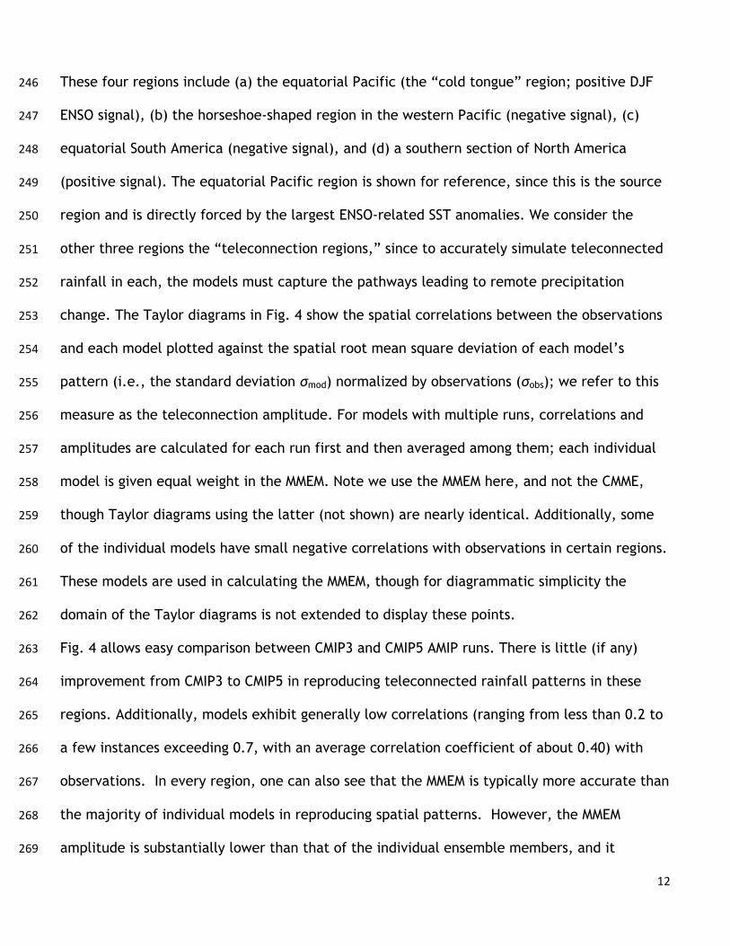
12
These four regions include (a) the equatorial Pacific (the “cold tongue” region; positive DJF 246
ENSO signal), (b) the horseshoe-shaped region in the western Pacific (negative signal), (c) 247
equatorial South America (negative signal), and (d) a southern section of North America 248
(positive signal). The equatorial Pacific region is shown for reference, since this is the source 249
region and is directly forced by the largest ENSO-related SST anomalies. We consider the 250
other three regions the “teleconnection regions,” since to accurately simulate teleconnected 251
rainfall in each, the models must capture the pathways leading to remote precipitation 252
change. The Taylor diagrams in Fig. 4 show the spatial correlations between the observations 253
and each model plotted against the spatial root mean square deviation of each model’s 254
pattern (i.e., the standard deviation σmod) normalized by observations (σobs); we refer to this 255
measure as the teleconnection amplitude. For models with multiple runs, correlations and 256
amplitudes are calculated for each run first and then averaged among them; each individual 257
model is given equal weight in the MMEM. Note we use the MMEM here, and not the CMME, 258
though Taylor diagrams using the latter (not shown) are nearly identical. Additionally, some 259
of the individual models have small negative correlations with observations in certain regions. 260
These models are used in calculating the MMEM, though for diagrammatic simplicity the 261
domain of the Taylor diagrams is not extended to display these points. 262
Fig. 4 allows easy comparison between CMIP3 and CMIP5 AMIP runs. There is little (if any) 263
improvement from CMIP3 to CMIP5 in reproducing teleconnected rainfall patterns in these 264
regions. Additionally, models exhibit generally low correlations (ranging from less than 0.2 to 265
a few instances exceeding 0.7, with an average correlation coefficient of about 0.40) with 266
observations. In every region, one can also see that the MMEM is typically more accurate than 267
the majority of individual models in reproducing spatial patterns. However, the MMEM 268
amplitude is substantially lower than that of the individual ensemble members, and it 269

13
underestimates the observations in every region outside of the central equatorial Pacific. As 270
a final point, we note that Taylor diagrams of the corresponding rank correlation method (not 271
shown) also indicate consistent results. 272
273
d. Teleconnection amplitude in major impact regions 274
The varied agreement in amplitude measures from Fig. 4 suggests that it may be more 275
reasonable to use amplitude information from individual ensemble members, rather than 276
using that of the MMEM. To get a better sense of how teleconnection amplitude of individual 277
models might be affected by internal variability within the models themselves, we take 278
advantage of AMIP models with multiple realizations, and we assess the internal variability 279
among these runs for each model. We then compare this to the amplitude range of the 15-280
model ensemble. Fig. 5 displays the radial axis from the Taylor diagrams discussed previously, 281
but where multiple runs from each model are available, we plot them individually (43 total 282
runs for 15 models in CMIP5; 26 total runs for 13 models in CMIP3; see Table 1). 283
The vertical extent of the black lines in Fig. 5, representing ± one standard deviation of the 284
amplitudes for the runs of a given model, is a measure of internal variability for that model. 285
The vertical extent of each green bar is ± one standard deviation of the MMEM amplitude, and 286
it serves as a measure of intermodel variability. Notable points from this diagram include: 287
(1) The MMEM systematically underestimates the spread and central tendency of intermodel 288
variability, with a low bias of about 20-40% outside of the immediate ENSO region; (2) the 289
regional disagreement among models owes itself partly to internal model variability, but 290
intermodel variability contributes to the majority of the regional disagreement seen in Fig. 3; 291
(3) individual models are overestimating the amplitude in the immediate ENSO region for 292
CMIP5, even though their spread is more symmetric about the observations in remote regions; 293

14
(4) when comparing CMIP5 to CMIP3, CMIP5 shows no consistent improvement or change due 294
to model development. Although the MMEM may fall closer to observed amplitudes in some 295
regions for CMIP5, this comes at the expense of a tendency for individual models to 296
overestimate rainfall teleconnections in the central ENSO region. 297
Fig. 5 suggests that serious errors can result from considering only information available in the 298
MMEM. While its spatial patterns correlate better with observations than most individual 299
models, the MMEM teleconnection amplitude is routinely too low in the remote regions 300
considered. It is therefore useful to consider measures of teleconnection amplitude and 301
spread from individual models, in addition to the MMEM, in situations where regional 302
disagreement can dampen the MMEM amplitudes due to averaging varied model signals. 303
304
4. Sign agreement plots in ENSO teleconnections, and an argument for agreement plots of 305
precipitation change in global warming scenarios 306
Agreement plots for the sign of precipitation change under global warming scenarios are 307
commonly used in multi-model studies (e.g., Randall et al. 2007; Meehl et al. 2007), often as 308
complementary information to the MMEM. Agreement-on-sign tests can be viewed as 309
relatively weak statements regarding the precipitation change at individual gridpoints for the 310
model ensemble, and it has been argued that sign agreement should be used in conjunction 311
with requirements on individual models that gridpoints pass statistical significance tests for 312
change in mean precipitation (e.g., Neelin et al. 2006; Tebaldi et al. 2011, hereafter N06 and 313
T11, respectively). 314
Here we examine agreement-on-sign measures based on the ENSO precipitation regression 315
patterns for each model. Because we can assess these against observations, we can use this to 316
examine the procedure as a means of inferring its usefulness. If a procedure that identifies 317

15
high model agreement at a gridpoint also correctly predicts the sign of the observations at 318
that gridpoint, it can help build confidence in using corresponding procedures for the global 319
warming case. 320
Fig. 6a shows the traditional agreement-on-sign plot for ENSO teleconnections in the CMIP5 321
AMIP ensemble. At each gridpoint, we count the number of models that agree on a positive 322
(negative) DJF teleconnection signal for the linear regression over Niño 3.4, so that the plot 323
shows the integer value of models which agree on a wet (dry) response during ENSO. The sign 324
of the regression slope at each gridpoint is equivalent to the sign of the expected DJF 325
precipitation response during an El Niño event. Areas with 12 or more models agreeing on 326
sign are shaded based on a binomial test. Specifically, if we consider the null hypothesis that 327
the value of an ENSO precipitation signal for a given point is equally likely to be positive or 328
negative, i.e. drawn from a binomial distribution with a probability of p=0.5, then when 12 or 329
more models agree on sign, the null hypothesis for this 50-50 probability can be rejected at a 330
confidence level greater than 95% (for 15 models, the 95% confidence level falls between an 331
agreement count of 10 and 11). 332
The gridpoints with high sign agreement that pass the binomial test at the 95% level in Fig. 6a 333
cover a spatial region similar to the areas passing the two-tailed t-test applied to the CMME 334
(Fig. 1d) at the 95% level. However, the areas of high sign agreement cover a much larger 335
spatial region than those passing the t-test at the 95% level for individual model realizations, 336
which are similar to the areas passing the t-test at this level for observations (see Fig. 1c and 337
the discussion in section 3a). 338
This last point suggests two comparisons. First, we can contrast regions of high sign 339
agreement identified by the binomial test with examples of criteria that have been 340
considered in the global warming literature that combine t-tests on individual models with 341

16
sign agreement criteria from the ensemble. Second, in this ENSO teleconnection testbed, we 342
can evaluate the model ensemble’s sign prediction against observations. These results are 343
displayed in Figs. 6b and 6c. These panels display hatching according to the N06 or T11 344
criteria, respectively, overlaid on a plot that assesses the prediction of the model ensemble 345
for the sign of the teleconnection signal; details of these criteria are outlined below. 346
To produce the cross-hatching in Fig. 6b, we follow the N06 procedure: (1) at each gridpoint, 347
count the number of models in the ensemble that have a slope significantly different from 348
zero at the 95% confidence interval; (2) cross-hatch grid points where greater than 50% of 349
models are significant and also agree on the sign of the precipitation teleconnection. The N06 350
criteria impose a requirement that at least half of models both be significant and agree on 351
sign. 352
To produce the cross-hatching in Fig. 6c, we follow the T11 procedure: (1) at each gridpoint, 353
count the number of models with a teleconnection significant at the 95% confidence interval 354
(as in N06); (2) for gridpoints where more than 50% of models show a significant rainfall 355
response, cross-hatch if 80% or more of significant models agree on the sign of the response; 356
(3) if fewer than 50% of models agree on the sign, shade the gridpoint black. 357
The underlying color shading in Figs. 6b and 6c is identical and evaluates the sign prediction 358
of the AMIP CMME for the teleconnection signal, produced in the following way: (1) take the 359
regions of high sign agreement passing the binomial test at the 95% significance level in Fig. 360
6a as a prediction of the sign of the observed teleconnection pattern and compare that to the 361
observations at the same gridpoint; (2) if the observations and the model prediction agree on 362
sign, shade blue (red) for a positive (negative) ENSO precipitation signal, representing a 363
correct prediction by the intermodel agreement plot (Fig. 6a); (3) if the observations and the 364
Fig. 6a disagree on the sign, shade the gridpoint purple to indicate an erroneous prediction; 365

17
(4) if the agreement on sign does not pass the binomial test criterion of Fig. 6a, no prediction 366
is made and the gridpoint is left unshaded. 367
When examining Figs. 6b and 6c, the most important point is that the model ensemble 368
prediction of sign does very well when assessed against observations. In major regions for 369
which model agreement passes the binomial test at 95% confidence, almost the whole area 370
yields the correct sign. The scattered, incorrect gridpoints tend to be either isolated or at the 371
edges of correct regions, such that a scientific assessment of likely areas of increase or 372
decrease based on the predicted areas (color shading in Figs. 6a and 6b) would be highly 373
accurate. Potential physical mechanisms for the success of the sign prediction are discussed in 374
the next section. 375
Another obvious point in Fig 6b and 6c is the similarity between the N06 and T11 approaches. 376
In practice, the T11 test employed here is equivalent to the N06 test defined at a 40% 377
threshold (80% x 50% = 40%). The one difference is that T11 further specify those grid points 378
where more than 50% of models are significant but fewer than 80% agree on sign, which they 379
classify as “no prediction.” This last T11 criterion may be useful in evaluating precipitation 380
change under global warming, where at a given gridpoint, statistical significance of the 381
precipitation change for individual models does not necessarily mean they will agree on sign. 382
In comparing the N06 and T11 procedures to the regions over which the models correctly 383
predict sign of the observations, it is immediately apparent that the N06 and T11 tests are 384
highly conservative. Though they do remove the modest fraction of points for which the sign 385
would have been incorrectly predicted based on high agreement (passing the binomial test at 386
the 95% level), they do so at the cost of excluding substantial regions that are correctly 387
predicted. This is evident in Figs. 6b and 6c, where the hatched areas are restricted in spatial 388
extent relative to the broader shaded regions. 389

18
To show the sign agreement of the model ensemble with observations in more detail, we 390
display in Fig. 7a the number of individual ensemble members that agree on sign with 391
observations for ENSO teleconnections. The same criterion for displaying high model 392
agreement (12 or more models) is used as in Fig. 6a. Within this region, it may be seen that 393
there are large portions in which the number of models agreeing on sign with observations is 394
even higher, including substantial areas where 100% of models agree with the sign of the 395
observations. 396
To obtain a counterpart of this plot from the model ensemble, Fig. 7b shows the number of 397
models agreeing with the sign of the MMEM. Note that in producing this, we exclude each 398
model’s contribution to the MMEM when determining agreement, so as to avoid inflating the 399
count. The similarities between Figs. 7a and 7b indicate that high sign agreement with the 400
MMEM can serve as a predictor for sign agreement with the observations. 401
402
5. Discussion 403
As discussed in the previous section, Figs. 6 and 7 suggest that there are substantial regions 404
where models from the CMIP5 AMIP ensemble are providing useful information on the sign of 405
rainfall teleconnections, despite individual models and the observations failing to meet t-test 406
criteria at the 95% level in parts of these regions. We argue below that this is a combined 407
consequence of the larger size of the model ensemble relative to individual runs, the nature 408
of the quantity being tested (the sign), and the models’ skill in predicting the observed sign. 409
Before addressing this, we consider the possibility that the broader region of skill at sign 410
prediction in the ensemble (relative to individual model runs) could simply be an issue with 411
applicability of the t-test due to the inherent non-Gaussianity of the rainfall distribution, 412
even at seasonal timescales. This was addressed in Fig. 2 by repeating the teleconnection 413

19
calculations using Spearman’s rank correlation, which makes no assumptions of Gaussianity 414
for the gridpoint rainfall distributions, and an accompanying statistical significance test. This 415
yields results similar to those of the linear regression t-test. 416
We now consider an explanation based on the fact that the sign agreement both uses 417
information from the full model ensemble and tests a different hypothesis than difference 418
from zero. Because the collective 15-model ensemble contains a much larger set of 419
realizations of internal variability, it is natural that regions of smaller signal should pass a 420
given significance criteria in measures that use all 15 models. This is evident in comparing 421
Fig. 6a to Fig. 1d, where areas of high sign agreement (passing the binomial test at the 95% 422
level) tend to coincide with areas that pass a t-test on the CMME at 95% confidence. In both 423
cases the broad regions of statistical significance come from using all 15 models. 424
Taking this into account, we consider the question of why the models agree so well with the 425
observations on the sign of the teleconnection patterns, despite doing poorly at detailed 426
spatial distribution. There are two aspects to this question: one statistical, and the other 427
physical. The statistical aspect is that where the models exhibit sign agreement of 80%, the 428
best estimate of the parameter p in the binomial distribution is 0.8. While it is beyond the 429
scope of the paper to establish Bayesian posterior probability density functions or other 430
measures of margin of error on the inferred p, the point needed to interpret the results here 431
is straightforward: if the models are sufficiently good representations of observations such 432
that the observed signal can be considered to be drawn from a binomial distribution with a 433
similar value of p at each point, then one would expect the high level of agreement seen. 434
Thus the 15-model ensemble shows success at predicting the sign of the observations in 435
broader regions than those where teleconnection signals pass t-tests applied to individual 436
models or observations. If we consider the fact that these broader regions are those that pass 437

20
the 95% confidence level of the binomial test, this success of the ensemble at sign prediction 438
is completely consistent with expectations and with the statement that the models are doing 439
well at simulating the observed sign. 440
The ability of models to provide information beyond what a particular significance test may 441
suggest is not a new concept in modeled precipitation studies. Risbey et al. (2011) resolve 442
significant teleconnections in an AMIP model using a 30-year record and a two-tailed t-test. 443
The authors note that the number of gridpoints passing a 95% significance criterion is much 444
fewer than the same method applied to a century of historical data. As a result, they loosen 445
their restriction to an 80% confidence interval, noting that the associated teleconnection 446
patterns are similar for records of either length. Power et al. (2012) evaluate projected 447
precipitation changes from the coupled CMIP3 model ensemble, and they demonstrate using 448
the binomial distribution that model consensus on the sign of end-of-century rainfall 449
anomalies is itself a strong argument for confidence in ensemble agreement patterns. 450
That the ensemble does, in fact, get broad areas of small amplitude change correct in our 451
teleconnection analysis adds to the discussion in the literature that projected change is worth 452
assessing even in regions that do not meet t-test criteria applied to individual runs (Tebaldi et 453
al. 2011, Power et al. 2012) if these regions do meet significance tests applied to the 454
ensemble. This is particularly relevant in global warming studies, where a modest regional 455
precipitation anomaly in a MMEM could mean substantial changes in regional precipitation 456
budgets. 457
An important physical question that arises from the present teleconnection results is: why 458
does the 15-model ensemble perform better at predicting the sign of the observed signal 459
(including in broad areas of modest precipitation amplitude response) and at yielding the 460
amplitude of the observed response than the individual models do at reproducing detailed 461

21
spatial patterns of observed teleconnections? The unimpressive spatial correlations (Fig. 4) 462
are affected by poor individual model skill in positioning high amplitude signals. 463
We suggest that this may be associated with the multiple physical processes operating in ENSO 464
teleconnections. Specifically, there are atmospheric processes at work that will have smaller 465
intermodel uncertainty and smaller internal variability but are widespread spatially. 466
Examples for these processes include an increase in tropospheric temperature driving changes 467
in radiative fluxes, as well as driving an increase in water vapor and a corresponding increase 468
in the threshold for convection (the thermodynamic process sometimes referred to as the 469
“rich-get-richer” mechanism; Chou and Neelin 2004; Held and Soden 2006; Trenberth 2011). 470
At the same time, feedbacks associated with dynamical changes in moisture convergence can 471
produce large excursions from expected values of precipitation, both in intermodel and 472
temporal variability. The models contain reasonable approximations to each of these 473
processes, but the location of strong precipitation changes can be highly sensitive to factors 474
such as model convection parameterizations, including the threshold for convective onset 475
(Kanamitsu et al. 2002; Neelin et al. 2010). 476
477
6. Summary and conclusions 478
AMIP runs from the CMIP3 and CMIP5 ensembles provide one standard by which we can judge 479
the ability of the CGCMs’ atmospheric components to reproduce dynamic feedback processes 480
that lead to remote seasonal precipitation anomalies. We focus on standard teleconnection 481
patterns associated with the ENSO Niño 3.4 index. Comparisons among the ensemble of 482
models and with the observations are made using precipitation teleconnection patterns for 483
the DJF for the years 1979-2005. The spatial patterns and amplitudes of these 484
teleconnections are analyzed in several regions with robust ENSO feedbacks, including the 485

22
eastern tropical Pacific, the “horseshoe” region in the western tropical Pacific, a southern 486
section of N. America, and equatorial S. America. 487
Teleconnection patterns are examined using three methods: linear regression, Spearman’s 488
rank correlation, and compositing techniques (not shown), all with similar results. The rank 489
correlation method provides an alternative significance test, which is useful in narrowing 490
some of the questions that arise for regions of low amplitude signal. Teleconnection patterns 491
defined with linear regression are useful for questions that involve the amplitude of the 492
signal; as such, we focus on results from the linear regression. 493
How well the models perform at reproducing the observed teleconnection patterns 494
(amplitudes and spatial patterns) depends strongly on the quantity for which they are 495
assessed. In standard measures of spatial correlation, taken over the regions outlined above, 496
the CMIP3 and CMIP5 AMIP models exhibit strong regional disagreement with one another and 497
with observations. Comparing patterns visually, this is associated with regions of strong 498
precipitation change varying substantially from model to model and with respect to 499
observations, yielding low spatial correlations between modeled and observed teleconnection 500
patterns (average correlation coefficients on the order of 0.40 in the defined regions). 501
The MMEM performs marginally better than most individual models in spatial correlation 502
measures, largely because the regions of strongest and varying change have been smoothed. 503
However, the MMEM systematically underestimate amplitude measures of the regional 504
precipitation response by 30-40%, typically falling more than one standard deviation below 505
the central tendency of the 15-model ensemble. This underestimation is again associated 506
with regional disagreement among ensemble members, a well-documented artifact in 507
precipitation studies of GCM ensembles (e.g., N06; Räisänen 2007; Knutti et al. 2010; Neelin 508
et al. 2010; Schaller et al. 2011). The average of individual CMIP5 AMIP amplitudes, by 509

23
contrast, is an accurate predictor for the observations in all regions but the central ENSO 510
region, where models overestimate the precipitation response. Sizeable internal variability of 511
precipitation teleconnections is also shown to exist within each model, though it does not 512
dominate the intermodel spread. 513
One thing underlined by the low spatial correlations in individual models is that even in AMIP 514
experiments, where only the atmospheric components of CGCMs are being compared, 515
simulation of ENSO teleconnections is fairly challenging for the models. While coupled models 516
will have additional feedbacks, the AMIP experiments provide a first line of assessment. 517
Furthermore, because we can compare AMIP simulations to observations, we can assess how 518
the model simulations fare under other metrics commonly used in assessment of ensemble 519
patterns and intermodel agreement 520
Sign agreement measures for a precipitation response in model ensembles are often used for 521
assessing global warming precipitation changes. Examining sign agreement for the 522
teleconnection patterns, the model ensemble has broad spatial regions with high consensus on 523
sign, passing a binomial test (to reject the null hypothesis of 50-50 probability of either sign) 524
at the 95% level. These regions are more spatially extensive than the regions for which 525
individual models (or observations) would pass a two-tailed t-test at the 95% (or even the 90%) 526
level. Furthermore, the regions passing the binomial test correspond well to the set of points 527
passing a t-test (at the 95% level) applied to the 15-model ensemble. Thus the larger region 528
with high agreement on sign, relative to regions passing criteria (e.g., N06 or T11) that make 529
use of t-tests on individual models, is simply the result of the sign agreement test making use 530
of the 15-model ensemble. 531
For these teleconnection patterns, the sign prediction can be tested against observations. The 532
models exhibit high sign agreement with observations over similarly broad regions, implying 533

24
that high sign agreement within the model ensemble (gridpoints passing the binomial test at 534
the 95% level) is a good predictor for sign agreement with observations. One can infer from 535
this that the model ensemble is producing useful information regarding the teleconnected 536
precipitation signal in regions that do not pass a t-test at the 95% level for individual models, 537
provided they pass a significance test that makes use of information from the full ensemble. 538
The evaluation of the model simulations for ENSO teleconnections may be used, with due 539
caution, to draw inferences for assessment of precipitation in global warming projections. 540
Many of the physical processes leading to rainfall teleconnections are analogous to the global 541
warming case. In particular, widespread tropospheric warming initiates tropical dynamics that 542
cause similar global precipitation change in both teleconnections and global warming. In both 543
cases, one can trace localized precipitation anomalies with high amplitude and sizeable 544
intermodel spread back to tropical regions of strong convergence feedbacks and regions 545
where large-scale wave dynamics interacts with mid-latitude storm tracks. 546
The unimpressive skill of models at capturing the precise regional distribution of large-547
amplitude rainfall teleconnections compared to observations is consistent with poor 548
intermodel agreement on a precise pattern of precipitation change in global warming. 549
However, the skill of individual models at reproducing the observed teleconnection signal 550
amplitude (assessed from the mean of the individual model amplitudes, not the MMEM) 551
suggests that corresponding measures for global warming precipitation change may be 552
trustworthy. Furthermore, sign agreement plots for the AMIP ensemble prove skillful at 553
predicting the sign of observed teleconnections. While agreement plots for end-of-century 554
precipitation change obviously have different spatial patterns than the signals considered 555
here, the fact that sign agreement plots are skillfull at predicting spatially extensive ENSO 556
remote precipitation impacts — which are challenging simulation targets that share physical 557

25
pathways with global warming precipitation signals — provides a supporting argument in favor 558
of using sign agreement plots in global warming studies to make predictions of change from an 559
ensemble of models.560

26
Acknowledgements. This work was supported in part by the NOAA Climate Program Office 561
Modeling, Analysis, Predictions and Projections (MAPP) Program under grant NA11OAR4310099 562
as part of the CMIP5 Task Force and National Science Foundation grant AGS-1102838. We 563
thank M. Münnich for insights into the behavior of rank correlation estimates of 564
teleconnections. CMAP precipitation data and NOAA_ERSST_V3 SST data are provided by the 565
NOAA/OAR/ESRL PSD, Boulder, Colorado, USA, from their website at 566
http://www.esrl.noaa.gov/psd/. We acknowledge the World Climate Research Programme's 567
Working Group on Coupled Modelling, which is responsible for CMIP, and we thank the climate 568
modeling groups for producing and making available their model output. For CMIP, the U.S. 569
Department of Energy's Program for Climate Model Diagnosis and Intercomparison provided 570
coordinating support and led development of software infrastructure in partnership with the 571
Global Organization for Earth System Science Portals. Finally, we thank J. Meyerson for her 572
significant help in data analysis and plotting.573

27
References 574
AchutaRao, K., and K. Sperber, 2006: ENSO simulations in coupled ocean-atmosphere models: 575
Are the current models better? Climate Dyn., 27, 1–16. 576
Ashok, K., S. K. Behera, S. A. Rao, H. Weng, and T. Yamagata, 2007: El Niño Modoki and its 577
possible teleconnection. J. Geophys. Res., 112, C11007. 578
Cai, W., A. Sullivan, and T. Cowan, 2009: Rainfall teleconnections with Indo-Pacific variability 579
in the WCRP CMIP3 models. J. Climate, 22, 5046–5071. 580
Cai, W., M. Lengaigne, S. Borlace, M. Collins, T. Cowan, M. J. McPhaden, A. Timmermann, S. 581
Power, J. Brown, C. Menkes, A. Ngari, E. M. Vincent, and M. J. Widlansky, 2012: More 582
extreme swings of the South Pacific convergence zone due to greenhouse warming. Nature, 583
488, 365-369. 584
Capotondi, A., A. Wittenberg, and S. Masina, 2006: Spatial and temporal structure of Tropical 585
Pacific interannual variability in 20th century coupled simulations. Ocean Modell., 15, 274. 586
Cash, B. A., E. K. Schneider, and L. Bengtsson, 2005: Origin of regional climate differences: 587
role of boundary conditions and model formulation in two GCMs. Climate Dyn., 25, 709-723. 588
Chen, W. Y, and H. M. van den Dool, 1997: Asymmetric impact of tropical SST anomalies on 589
atmospheric internal variability over the North Pacific. J. Atmos. Sci., 54, 725-740. 590
Chiang, J. C. H., and A. H. Sobel, 2002: Tropical tropospheric temperature variations caused 591
by ENSO and their influence on the remote tropical climate. J. Climate, 15, 2616–2631. 592
Chou, C., and J. D. Neelin, 2004: Mechanisms of global warming impacts on regional tropical 593
precipitation. J. Climate, 17, 2688–2701. 594
Coelho, Caio A. S., and L. Goddard, 2009: El Niño–Induced Tropical Droughts in Climate 595
Change Projections. J. Climate, 22, 6456–6476. 596
Collins, M., and Coauthors, 2010: The impact of global warming on the tropical Pacific Ocean 597

28
and El Niño. Nat. Geosci., 3, 391–397. 598
Dai, A. and T. M. L. Wigley, 2000: Global patterns of ENSO-induced Precipitation. Geophys. 599
Res. Lett., 27, 1283-1286. 600
Dai, A., 2006: Precipitation Characteristics in Eighteen Couple Climate Models. J. Climate, 601
19, 4605-4630. 602
Davey, M., and Coauthors, 2001: STOIC: A study of coupled model climatology and variability 603
in tropical regions. Climate Dyn., 18, 403–420. 604
Delecluse, P., M. K. Davey, Y. Kitamura, S. G. H. Philander, M. Suarez, and L. Bengtsson, 605
1998: Coupled general circulation modeling of the tropical Pacific. J. Geophys. Res., 103 606
(C7), 14 357–14 373. 607
DeWeaver, E., and S. Nigam, 2004: On the forcing of ENSO teleconnections by anomalous 608
heating and cooling. J. Climate,17, 3225-3235. 609
Doherty, R. and M. Hulme, 2002: The relationship between the SOI and extended tropical 610
precipitation in simulations of future climate change. Geophys. Res. Lett., 29, 1475. 611
Gates, W. L., and Coauthors, 1998: An overview of the results of the Atmospheric Model 612
Intercomparison Project (AMIP I). Bull. Amer. Meteor. Soc., 73, 1962–1970. 613
Guilyardi, E., and Coauthors, 2004: Representing El Niño in coupled ocean–atmosphere GCMs: 614
The dominant role of the atmospheric component. J. Climate, 17, 4623–4629. 615
Guilyardi, E., A. Wittenberg, A. Fedorov, M. Collins, C. Wang, A. Capotondi, G. van 616
Oldenborgh, and T. Stockdale, 2009a: Understanding El Niño in ocean–atmosphere general 617
circulation models: Progress and challenges. Bull. Amer. Meteor. Soc., 90, 325–340. 618
Guilyardi, E., P. Braconnot, F.-F. Jin, S. T. Kim, M. Kolasinski, T. Li, and I. Musat, 2009b: 619
Atmosphere feedbacks during ENSO in a coupled GCM with a modified atmospheric convection 620
scheme. J. Climate, 22, 5698–5718. 621

29
Held, I. M., S. W. Lyons, and S. Nigam, 1989: Transients and the extratropical response to El 622
Niño. J. Atmos. Sci., 46, 163-174. 623
Held, I. M., and B. J. Soden, 2006: Robust responses of the hydrological cycle to global 624
warming. J. Climate, 19, 5686– 5699. 625
Horel, J. D., and J. M. Wallace, 1981: Planetary-scale atmospheric phenomena associated 626
with the Southern Oscillation. Mon. Wea. Rev., 109, 813–829. 627
Joseph, R., and S. Nigam, 2006: ENSO evolution and teleconnections in IPCC’s Twentieth-628
Century climate simulations: Realistic representation? J. Climate, 19, 4360-4377. 629
Kao, H.-Y., and J.-Y. Yu, 2009: Contrasting eastern-Pacific and central-Pacific types of ENSO. 630
J. Climate, 22, 615–632. 631
Kanamitsu, M., and Coauthors, 2002: NCEP dynamical seasonal forecast system 2000. Bull. 632
Amer. Meteor. Soc, 83, 1019–1037. 633
Knutti, R., R. Furrer, C. Tebaldi, J. Cermak, and G. A. Meehl, 2010: Challenges in combining 634
projections from multiple climate models. J. Climate, 23, 2739–2758. 635
Latif, M., and Coauthors, 2001: ENSIP: The El Niño Simulation Intercomparison Project. 636
Climate Dyn., 18, 255–272. 637
Lloyd, J., E. Guilyardi, H. Weller, and J. Slingo, 2009: The role of atmosphere feedbacks 638
during ENSO in the CMIP3 models. Atmos. Sci. Lett., 10, 170–176. 639
Meehl, G. A., and Coauthors, 2007: Global climate projections. Climate Change 2007: The 640
Physical Science Basis, S. Solomon, et al., Eds., Cambridge University Press, 747–845. 641
Meehl, G. A., and H. Teng, 2007: Multi-model changes in El Niño teleconnections over North 642
America in a future warmer climate. Climate Dyn., 29, 779-790. 643
Merryfield, W., 2006: Changes to ENSO under CO2 doubling in a multimodel ensemble. J. 644
Climate, 19, 4009–4027. 645

30
Münnich, M., and J. D. Neelin, 2005: Seasonal influence of ENSO on the Atlantic ITCZ and 646
equatorial South America. Geophys. Res. Lett., 32, L21709. 647
Neelin, J. D., and Coauthors, 1992: Tropical air–sea interaction in general circulation models. 648
Climate Dyn., 7, 73–104. 649
Neelin, J. D., C. Chou, and H. Su, 2003: Tropical drought regions in global warming and El 650
Niño teleconnections. Geophys. Res. Lett., 30, 2275. 651
Neelin, J. D., M. Münnich, H. Su, J. E. Meyerson, and C. E. Holloway, 2006: Tropical drying 652
trends in global warming models and observations. Proc. Natl. Acad. Sci., 103, 6110-6115. 653
Neelin, J. D., A. Bracco, H. Luo, J. C. McWilliams, and J. E. Meyerson, 2010: Considerations 654
for parameter optimization and sensitivity in climate models. Proc. Natl. Acad. Sci., 107, 21 655
349–21 354. 656
Oldenborgh, G.J. van, and T. Stockdale, 2009: Understanding El Niño in Ocean-Atmosphere 657
General Circulation Models: Progress and challenges. Bull. Amer. Met. Soc., 90, 325-340. 658
Power, S. B., F. Delage, R. Colman, and A. Moise, 2012: Consensus on Twenty-First-Century 659
Rainfall Projections in Climate Models More Widespread than Previously Thought. J. Climate, 660
25, 3792-3809. 661
Räisänen, J., 2007: How reliable are climate models? Tellus, 59A, 2–29. 662
Randall, D. A., and Coauthors, 2007: Climate models and their evaluation. Climate Change 663
2007: The Physical Science Basis, S. Solomon et al., Eds., Cambridge University Press, 589–664
662. 665
Risbey, J. S., P. C. McIntosh, M. J. Pook, H. A. Rashid, and A. C. Hirst, 2011: Evaluation of 666
rainfall drivers and teleconnections in an ACCESS AMIP run. Aust. Meteor. Oceanogr. J., 61, 667
91-105. 668
Ropelewski, C. F., and M. S. Halpert, 1987: Global and regional scale precipitation patterns 669

31
associated with the El Niño/ Southern Oscillation. Mon. Wea. Rev., 115, 1606–1626. 670
Schaller, N., I. Mahlstein, J. Cermak, and R. Knutti, 2011: Analyzing precipitation projections: 671
A comparison of different approaches to climate model evaluation. J. Geophys. Res., 116, 672
D10118. 673
Smith, T. M., R. W. Reynolds, T. C. Peterson, and J. Lawrimore, 2008: Improvements to 674
NOAA's historical merged land-ocean surface temperature analysis (1880-2006). J. Climate, 675
21, 2283-2296. 676
Spencer, H., and J. M. Slingo, 2003: The simulation of peak and delayed ENSO 677
teleconnections. J. Climate, 16, 1757–1774. 678
Straus, D. M., and J. Shukla, 1997: Variations of midlatitude transient dynamics associated 679
with ENSO. J. Atmos. Sci., 54, 777-790. 680
Su, H., J. D. Neelin, and J. E. Meyerson, 2003: Sensitivity of tropical tropospheric 681
temperature to sea surface temperature forcing. J. Climate, 16, 1283–1301. 682
Sun, D.-Z., Y. Yu, and T. Zhang, 2009: Tropical water vapor and cloud feedbacks in climate 683
models: A further assessment using coupled simulations. J. Climate, 22, 1287–1304. 684
Tebaldi, C., J. Arblaster, and R. Knutti, 2011: Mapping model agreement on future climate 685
projections. Geophys. Res. Lett., 38, L23701. 686
Trenberth, K. E., 1997: The Definition of El Niño. Bull. Amer. Met. Soc., 78, 2771-2777. 687
Trenberth, K. E., G. W. Branstator, D. Karoly, A. Kumar, N.-C. Lau, and C. Ropelewski, 1998: 688
Progress during TOGA in understanding and modeling global teleconnections associated with 689
tropical sea surface temperatures. J. Geophys. Res., 103, 14 291–14 324. 690
Trenberth, K. E., and L. Smith, 2009: Variations in the three-dimensional structure of the 691
atmospheric circulation with different flavors of El Niño. J. Climate, 22, 2978–2991. 692
Trenberth, K. E., 2011: Changes in precipitation with climate change. Clim. Res., 47, 123-693

32
138. 694
von Storch, H., and F. W. Zwiers, 1999: Statistical analysis in climate research. Cambridge 695
University Press, Cambridge. 696
Weare, B. C., 2012: El Niño teleconnections in CMIP5 models. Climate Dyn., published online, 697
doi:10.1007/s00382-012-1537-3. 698
Whitaker, J. S., and K. M. Weickmann, 2001: Subseasonal variations of tropical convection 699
and week-2 prediction of wintertime western North American rainfall. J. Climate, 14, 3279–700
3288 701
Wilks, D. S., 1995: Statistical Methods in the Atmospheric Sciences: An Introduction. 702
Academic Press, 467 pp. 703
Xie, P., and P. A. Arkin, 1997: Global Precipitation: A 17-year monthly analysis based on 704
gauge observations, satellite estimates, and numerical model outputs. Bull. Amer. Meteor. 705
Soc., 78, 2539– 2558. 706
Xue, Y., T. M. Smith, and R. W. Reynolds, 2003: Interdecadal changes of 30-yr SST normals 707
during 1871-2000. J. Climate, 16, 1601-1612. 708
709

33
Table 1. CMIP5 and CMIP3 modeling centers and models used, and the number of AMIP runs 710
available at the time of our analysis. Data are available for download at 711
http://pcmdi3.llnl.gov. 712
Modeling center or group (institute ID) CMIP5 AMIP model runs CMIP3 AMIP model runs Beijing Climate Center, China Meteorological Administration (BCC) BCC-CSM1.1 3
Canadian Centre for Climate Modelling and Analysis (CCCMA) CanAM4 4
National Center for Environmental Research (NCAR) CCSM4 1 CCSM3 1
PCM 1
Centro Euro-Mediterraneo per I Cambiamente Climatici (CMCC) CNRM-CM5 1 CNRM-CM3 1 Commonwealth Scientific and Industrial Research Organization in collaboration with Queensland Climate Change Centre of Excellence (CSIRO-QCCCE) CSIRO-Mk3.6.0 1
LASG, Institute of Atmospheric Physics, Chinese Academy of Sciences (LASG-CESS) FGOALS-s2 3 FGOALS-g1.0 3 NOAA Geophysical Fluid Dynamics Laboratory (NOAA GFDL) GFDL-HIRAM-C180 3 GFDL-CM2.1 1 NASA Goddard Institute for Space Studies (NASA GISS) GISS-E2-R 5 GISS-ER 4 Met Office Hadley Centre (MOHC) HadGEM2-A 5 UKMO-HadGEM1 1 Institute for Numerical Mathematics (INM) INM-CM4 1 INM-CM3.0 1 Institut Pierre-Simon Laplace (IPSL) IPSL-CM5A-LR 5 IPSL-CM4 5 Atmosphere and Ocean Research Institute (The University of Tokyo), National Institute for Environmental Studies, and Japan Agency for Marine-Earth Science and Technology (MIROC) MIROC5 2 MIROC3.2(hires) 1
MIROC3.2(medres) 3
Max Planck Institute for Meteorology (MPI-M) MPI-ESM-LR 3 ECHAM5/MPI-OM 3 Meteorological Research Institute (MRI) MRI-CGCM3 3 MRI-CGCM2.3.2 1 Norwegian Climate Centre (NCC) NorESM1-M 3

34
Figures and captions 713
180 120W 60W120E60E 180 120W 60W120E60E
30N
0
30S
180 120W 60W120E60E
-5 -2 -1 -0.5 -0.1 0
180 120W 60W120E60E
30N
0
30S
0.1 0.5 1 2 5Linear Regression (mm day-1 C-1)
(a) Observations (b) CMME
(c) Observations with significance test applied (d) CMME with significance test applied
714
Figure 1. DJF precipitation teleconnections for the years 1979-2005, as diagnosed through a linear regression 715
analysis of precipitation against the Niño 3.4 index (units of mm day-1 C-1). (a) Observed teleconnections. (b) 716
Concatenated multi-model ensemble (CMME) teleconnections for the CMIP5 AMIP 15-model ensemble. (c) Same 717
as in (a), but with a two-tailed t-test applied to the regression values and shaded at 95% confidence (black 718
outline) and 90% confidence (lighter shading). (d) Same as in (b) but shaded only where a t-test yields gridpoints 719
significant at or above the 95% confidence level.720

35
(a)
Spearman's Rank Correlation
(a) Observations (b) CMME
(c) Observations with significance test applied (d) CMME with significance test applied
-0.85-1 -0.6 -0.45 -0.2 -0.1 0 0.1 0.2 0.45 0.6 0.85 1-0.85-1 -0.6 -0.45 -0.2 -0.1 0 0.1 0.2 0.45 0.6 0.85 1
180 120W 60W120E60E 180 120W 60W120E60E
30N
0
30S
180 120W 60W120E60E 180 120W 60W120E60E
30N
0
30S
721
Figure 2. As in Fig. 1, but for Spearman’s rank correlation analysis between gridpoint precipitation and the Niño 722
3.4 index. Note here that the color bar is unitless and corresponds to the Spearman’s rank correlation 723
coefficient, with a minimum of -1.0 and a maximum of +1.0. Panels (a) and (b) show the teleconnection 724
patterns from the rank correlation applied to the observations and CMME, respectively. (c) Same as in (a) but 725
shaded only where gridpoints pass the 95% confidence level (black outline) and the 90% confidence level (lighter 726
shading) of a statistical significance test for the rank correlation analysis. (d) The CMME teleconnections shaded 727
for gridpoints that pass at the 95% significance level in the rank correlation analysis. 728
729

36
30N
0
30S
120W 60W 120W
-5 -2 -1 -0.5 -0.1 0(mm day-1 C-1)
0.1 0.5 1 2 5
60W 120W 60W 120W 60W
(m) MIROC5 (n) MPI-ESM-LR (o) MRI-CGCM3 (p) NorESM1-M
30N
0
30S
(i) GISS-E2-R (j) HADGEM2-A (k) INM-CM4 (l) IPSL-CM5A-LR
30N
0
30S
(e) CNRM-CM5 (f) CSIRO-Mk3.6.0 (g) FGOALS-s2 (h) GFDL-HIRAM-C180
30N
0
30S
(a) OBSERVATIONS (b) BCC-CSM1.1
(c) CanAM4 (d) CCSM4
730
Figure 3. DJF precipitation teleconnections shown for (a) the observations, top left, and (b)-(p) one run from 731
each of 15 available CMIP5 AMIP models (listed alphabetically by model acronym). Teleconnections here are 732
resolved via the linear regression analysis as in Fig. 1, with an identical color bar that has units of mm day-1 C-1. 733
Patterns are plotted for the equatorial Americas to highlight regional (intermodel) disagreement among the 734
ensemble members.735

37
2.0
1.6
1.2
0.8
0.4
0.4 0.8 1.2 1.6 2.0
0.10
0.20
0.30
0.40
0.50
0.60
0.70
0.80
0.90
0.95
0.99
Correlation
2.0
1.6
1.2
0.8
0.4
0.4 0.8 1.2 1.6 2.0
0.10
0.20
0.30
0.40
0.50
0.60
0.70
0.80
0.90
0.95
0.99
Correlation
2.0
1.6
1.2
0.8
0.4
0.4 0.8 1.2 1.6 2.0
0.10
0.20
0.30
0.40
0.50
0.60
0.70
0.80
0.90
0.95
0.99
Correlation
2.0
1.6
1.2
0.8
0.4
0.4 0.8 1.2 1.6 2.0
0.10
0.20
0.30
0.40
0.50
0.60
0.70
0.80
0.90
0.95
0.99
Correlation
CMIP3 ModelsCMIP3 MMEMCMIP5 ModelsCMIP5 MMEM
Eq. Pac. W. Pac.
S. Amer. N. Amer.
(a) (b)
(c) (d)
σm
od/σ
obs
σm
od/σ
obs
σmod/σobs σmod/σobs
σmod/σobs σmod/σobs
σm
od/σ
obs
σm
od/σ
obs
736
Figure 4. Taylor diagrams for the standardized amplitude and spatial correlation of precipitation teleconnections 737
in four selected regions, as indicated in the inset of each panel: (a) the equatorial Pacific (central ENSO) region, 738
(b) the “horseshoe” region in the western equatorial Pacific, (c) an equatorial section of South America, and (d) 739
a southern section of North America. On the Taylor diagrams, angular axes show spatial correlations between 740
modeled and observed teleconnections; radial axes show spatial standard deviation (root mean square deviation) 741
of the teleconnection signals in each area, normalized against that of the observations. Shaded red triangles (15 742
total) and blue circles (11 total) denote each of the CMIP5 and CMIP3 AMIP models, respectively. The unshaded 743
red triangle is the CMIP5 MMEM; the unshaded blue circle is the CMIP3 MMEM. Note that some models have 744
negative correlations with the observed teleconnections in a few regions, and while we include them in the 745
MMEM, we do not plot them individually in the diagrams.746

38
2.0
1.8
1.6
1.4
1.2
1.0
0.8
0.6
0.4
0.2
stand
ardiz
ed a
mplitu
deEq. Pac. W. Pac. S. Am. N. Am. Eq. Pac. W. Pac. S. Am. N. Am.
CMIP5 CMIP3 747
Figure 5. Standardized amplitude of precipitation teleconnections in each of the four regions identified in Fig. 4. 748
The calculation for this amplitude is discussed in the caption of Fig. 4 and in the text. CMIP5 models (15 models, 749
43 runs) are shown on the left; CMIP3 models (13 models, 26 runs) on the right; see Table 1 for models used. 750
Each blue dot represents a separate model run, and where multiple runs are available for a given model, a blue 751
dot is plotted for each. Black bars represent the spread among the multiple runs for one model (when available), 752
centered at that model’s average amplitude among the multiple runs (±1 standard deviation of the amplitude 753
measure). The green dots and green bars denote the average teleconnection amplitude and its spread (±1 754
standard deviation) for the entire ensemble, in each region. The red dot is the MMEM including all available 755
models and runs, weighted so that each separate model contributes equally.756

39
(a) Agreement on ENSO teleconnections
(b) Neelin et al. 2006 (N06) criteria and sign prediction assessment
(c) Tebaldi et al. 2011 (T11) criteria and sign prediction assessment
180 120W 60W 00 120E60E
180 120W 60W 00 120E60E
90N
60N
30N
0
30S
60S
90S
90N
60N
30N
0
30S
60S
90S
180 120W 60W 00 120E60E
90N
60N
30N
0
30S
60S
90S
1212 1313 1414 1515Model agreement
on negative anomaly
Correct pos. / neg. sign prediction Incorrect sign prediction
T11 criterion
N06 criterion
Model agreementon positive anomaly
757
Figure 6. (a) Agreement on a positive teleconnection signal (linear regression) within the 15-model ensemble. 758
Blue (red) colors represent high agreement on a positive (negative) precipitation response during ENSO events. 759
Note that in an ensemble of 15 models, an agreement count of 12 implies that 80% of models agree on the sign 760
of the precipitation teleconnection at that gridpoint, which is the area passing a binomial test at greater than 761
the 95% confidence level (discussed in text). (b) Neelin et al. 2006 (N06) significance criteria (cross-hatching) 762
overlaid on the sign prediction of the 15-model ensemble (colored shading). (c) Tebaldi et a. 2011 (T11) 763
significance criteria (cross-hatching) overlaid on the sign prediction of the ensemble, as in (b). Details of the N06 764
and T11 cross-hatching criteria and sign prediction shading are outlined in the text. The cross-hatching is shown 765
as an overlay in (b) and (c) to highlight the restrictive nature of the N06 and T11 criteria relative to the more 766
extensive spatial coverage over which the 15-model ensemble passes the binomial test at the 95% level and 767
exhibits an accurate prediction of the observed teleconnection signals.768

40
180 120W 60W120E60E
1212 1313 1414 1515
90N
60N
30N
0
30S
60S
90S
90N
60N
30N
0
30S
60S
90S
Model agreementon negative anomaly
Model agreementon positive anomaly
(b) Agreement with MMEM
(a) Agreement with observations
180 120W 60W 0120E60E0
1212 1313 1414 1515Model agreement
on negative anomalyModel agreement
on positive anomaly 769
Figure 7. (a) Sign agreement of precipitation teleconnections between each of 15 CMIP5 AMIP models and the 770
observations. (b) Sign agreement of precipitation teleconnections between the CMIP5 AMIP models and the 771
MMEM, calculated using one run from each model. For (b), each model is individually removed from the MMEM 772
before determining its sign agreement. Both (a) and (b) use Niño 3.4 teleconnection patterns diagnosed via 773
linear regression. Red areas denote models that agree with the observations or MMEM on a negative 774
precipitation signal during ENSO events; blue areas imply agreement on a positive precipitation signal. 775