1 Basic Definitions

A Problem is a relation from input to acceptable output. For example,

INPUT: A list of integers x1, . . . , xn

OUTPUT: One of the three smallest numbers in the list

An algorithm A solves a problem if A produces an acceptable output for EVERYinput.

A optimization problem has the following form: output a best solution S satis-fying some property P . A best solution is called an optimal solution. Note thatfor many problems there may be many different optimal solutions. A feasiblesolution is a solution that satisfies the property P . Most of the problems thatwe consider can be viewed as optimization problems.

2 Proof By Contradiction

A proof is a sequence S1, . . . , Sn of statements where every statement is eitheran axiom, which is something that we’ve assumed to be true, or follows logicallyfrom the precedding statements.

To prove a statement p by contradiction we start with the first statement of theproof as p̄, that is not p. A proof by contradiction then has the following form

p̄, . . . , q, . . . , q̄

Hence, by establishing that p̄ logically implies both a statement q and its nega-tion q̄, the only way to avoid logical inconsistency in your system is if p istrue.

Almost all proofs of correctness use proof by contradiction in one way or another.

3 Exchange Argument

Here we explain what an exchange argument is. Exchange arguments are themost common and simpliest way to prove that a greedy algorithm is optimalfor some optimization problem. However, there are cases where an exchangeargument will not work.

Let A be the greedy algorithm that we are trying to prove correct, and A(I)the output of A on some input I. Let O be an optimal solution on input I thatis not equal to A(I).

The goal in exchange argument is to show how to modify O to create a newsolution O′ with the following properties:

1

1. O′ is at least as good of solution as O (or equivalently O′ is also optimal),and

2. O′ is “more like” A(I) than O.

Note that the creative part, that is different for each algorithm/problem, isdetermininig how to modify O to create O′. One good heuristic to think ofA constructing A(I) over time, and then to look to made the modification atthe first point where A makes a choice that is different than what is in O. Inmost of the problem that we examine, this modification involves changing justa few elements of O. Also, what “more like” means can change from problemto problem. Once again, while this frequently works, there’s no guarantee.

4 Why an Exchange Argument is Sufficient

We give two possible proof techniques that use an exchange argument. The firstuses proof by contradiction, and the second is a more constructive argument.

Theorem: The algorithm A solves the problem.

Proof: Assume to reach a contradiction that A is not correct. Hence, theremust be some input I on which A does not produce an optimal solution. Letthe output produced by A be A(I). Let O be the optimal solution that is mostlike A(I).

If we can show how to modify O to create a new solution O′ with the followingproperties:

1. O′ is at least as good of solution as O (and hence O′ is also optimal), and

2. O′ is more like A(I) than O.

Then we have a contradiction to the choice of O.

End of Proof.

Theorem: The algorithm A solves the problem.

Proof: Let I be an arbitrary instance. Let O be arbitrary optimal solution forI. Assume that we can show how to modify O to create a new solution O′ withthe following properties:

1. O′ is at least as good of solution as O (and hence O′ is also optimal), and

2. O′ is more like A(I) than O.

Then consider the sequence O,O′′, O′′′, O′′′′, . . .

Each element of this sequence is optimal, and more like A(I) than the procedingelement. Hence, ultimately this sequence must terminate with A(I). Hence,A(I) is optimal.

End of Proof.

I personally prefer the proof by contradiction form, but it is solely a matter of

2

personal preference.

5 Proving an Algorithm Incorrect

To show that an algorithm A does not solve a problem it is sufficient to exhibitone input on which A does not produce an acceptable output.

6 Maximum Cardinality Disjoint Interval Prob-lem

INPUT: A collection of intervals C = {(a1, b1), . . . , (an, bn)} over the real line.

OUTPUT: A maximum cardinality collection of disjoint intervals.

This problem can be interpretted as an optimization problem in the followingway. A feasible solution is a collection of disjoint intervals. The measure ofgoodness of a feasible solution is the number of intervals.

Consider the following algorithm A for computing a solution S:

1. Pick the interval I from C with the smallest right endpoint. Add I to S.

2. Remove I, and any intervals that overlap with I, from C.

3. If C is not yet empty, go to step 1.

Theorem: Algorithm A correctly solves this problem.

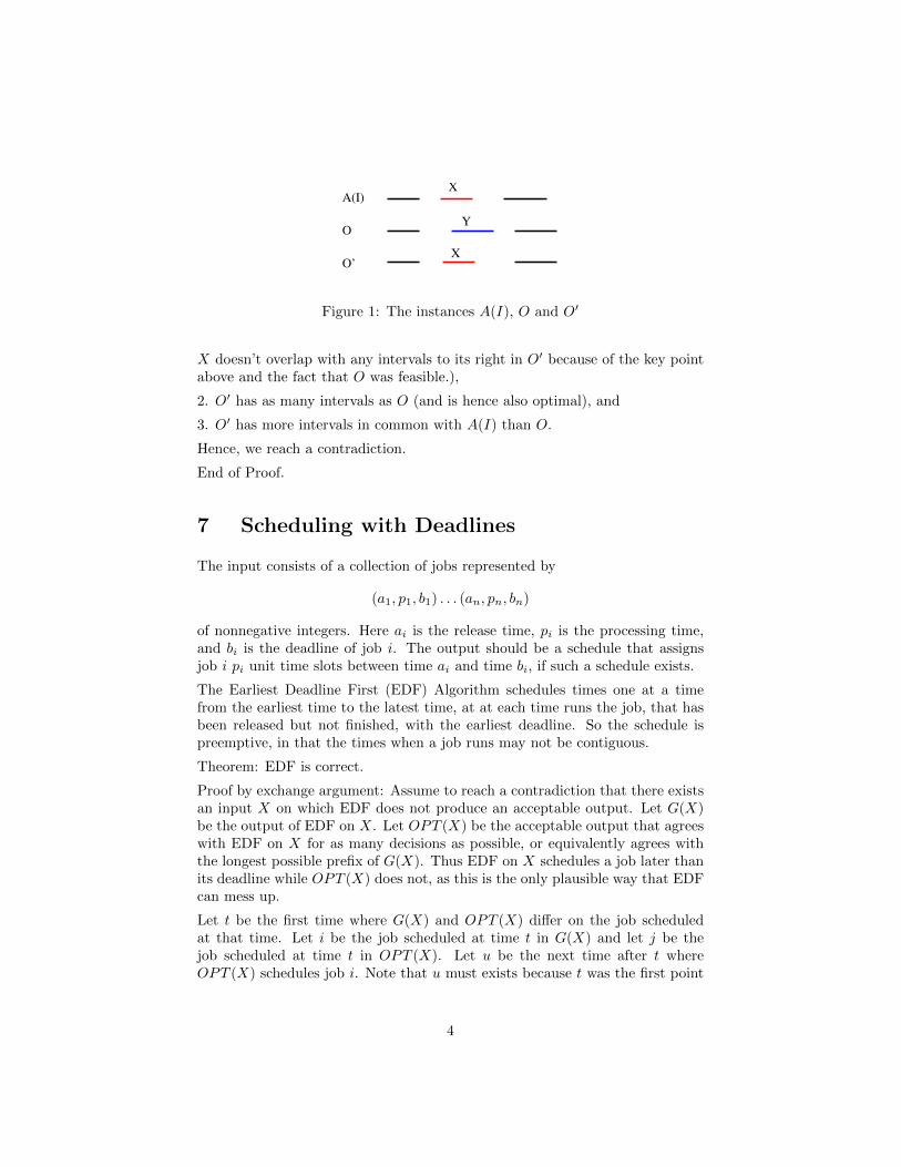
Proof: Assume to reach a contradiction that A is not correct. Hence, theremust be some input I on which A does not produce an optimal solution. Letthe output produced by A be A(I). Let O be the optimal solution that has themost number of intervals in common with A(I).

First note that A(I) is feasible (i.e. the intervals in A(I) are disjoint).

Let X be the leftmost interval in A(I) that is not in O. Note that such aninterval must exist otherwise A(I) = O (contradicting the nonoptimality ofA(I)), or A(I) is a strict subset of O (which is a contradiction since A wouldhave selected the last interval in O).

Let Y be the leftmost interval in O that is not in A(I). Such an interval mustexist or O would be a subset of A(I), contradiction the optimality of O.

The key point is that the right endpoint of X is to the left of the right endpointof Y . Otherwise, A would have selected Y instead of X.

Now consider the set O′ = O − Y + X.

We claim that:

1. O′ is feasible (To see this note that X doesn’t overlap with any intervals toits left in O′ because these intervals are also in A(I) and A(I) is feasible. And

3

A(I)

O

O’

X

Y

X

Figure 1: The instances A(I), O and O′

X doesn’t overlap with any intervals to its right in O′ because of the key pointabove and the fact that O was feasible.),

2. O′ has as many intervals as O (and is hence also optimal), and

3. O′ has more intervals in common with A(I) than O.

Hence, we reach a contradiction.

End of Proof.

7 Scheduling with Deadlines

The input consists of a collection of jobs represented by

(a1, p1, b1) . . . (an, pn, bn)

of nonnegative integers. Here ai is the release time, pi is the processing time,and bi is the deadline of job i. The output should be a schedule that assignsjob i pi unit time slots between time ai and time bi, if such a schedule exists.

The Earliest Deadline First (EDF) Algorithm schedules times one at a timefrom the earliest time to the latest time, at at each time runs the job, that hasbeen released but not finished, with the earliest deadline. So the schedule ispreemptive, in that the times when a job runs may not be contiguous.

Theorem: EDF is correct.

Proof by exchange argument: Assume to reach a contradiction that there existsan input X on which EDF does not produce an acceptable output. Let G(X)be the output of EDF on X. Let OPT (X) be the acceptable output that agreeswith EDF on X for as many decisions as possible, or equivalently agrees withthe longest possible prefix of G(X). Thus EDF on X schedules a job later thanits deadline while OPT (X) does not, as this is the only plausible way that EDFcan mess up.

Let t be the first time where G(X) and OPT (X) differ on the job scheduledat that time. Let i be the job scheduled at time t in G(X) and let j be thejob scheduled at time t in OPT (X). Let u be the next time after t whereOPT (X) schedules job i. Note that u must exists because t was the first point

4

of disagreement of OPT (X) and G(X), G(X) hadn’t finished job i by time t(and thus neither had OPT (X)), and OPT (X) is an acceptable output.

Figure 2: The instances G(X), Opt(X) and Opt′(X)

Let OPT ′(X) be equal to OPT (X) except that i is scheduled at time t and jis scheduled at time u. Obviously OPT ′(X) agrees with G(X) for at least onemore time unit than does OPT (X). OPT ′(X) is an acceptable output because:

• Each job is scheduled for the same amount of time as OPT (X)

• Job i can be feasibly run at time t because G(X) runs it at time t, andEDF would not have run i at time t if that was before i’s release time.

• Job j can be feasibly run at time u because:

– Job i can be feasibly run at time u because OPT (X) runs job i attime u, and OPT (X) is an acceptable output.

– Job’s i deadline is earlier than job j’s deadline because EDF selectedto run job i at time t, when running job j at time t was feasible.

But then we reach a contradiction to the definition of OPT (X) as OPT ′(X)is an acceptable output that agrees with G(X) for one more step than doesOPT (X).

5

End of Proof.

8 Shortest Remaining Processing Time (SRPT)

The input consists of a collection of jobs represented by

(a1, p1) . . . (an, pn)

of nonnegative integers. Here ai is the release time, and pi is the processingtime. The output should be a schedule that assigns job i pi unit time slots aftertime ai so as to minimize

∑i=1 ci, where the completion time ci is the first time

such that all pi units of job i have been processed.

The Shortest Remaining Processing Time (SRPT) Algorithm schedules timesone at a time from the earliest time to the latest time, at at each time runs thejob, that has been released but not finished, with the least remaining units toprocess until the job will be completed. So the schedule is preemptive, in thatthe times when a job runs may not be contiguous.

Theorem: SRPT is correct.

Proof by exchange argument: Assume to reach a contradiction that there existsan input X on which SRPT does not produce an acceptable output. Let G(X)be the output of SRPT on X. Let OPT (X) be the acceptable output that agreeswith SRPT on X for as many decisions as possible, or equivalently agrees withthe longest possible prefix of G(X).

Let t be the first time where G(X) and OPT (X) differ on the job scheduledat that time. Let i be the job scheduled at time t in G(X) and let j be thejob scheduled at time t in OPT (X). Let U be the collection of unit time slotsafter t where OPT (X) schedules either job i or job j. Note that during U thatOPT (X) schedules both jobs i and jobs j by the assumption that t is the firstpoint of disagreement for G(X) and OPT (X).

Let OPT ′(X) be equal to OPT (X) except during the unit time slots in U ;During the time slots in U first i is run to completion and then j is run.

Obviously OPT ′(X) agrees with G(X) for at least one more time unit thandoes OPT (X) as OPT ′(X) runs i at time t. OPT ′(X) is an acceptable outputbecause:

• Each job is scheduled for the same amount of time as OPT (X)

• Job i can be feasibly run at time t because G(X) runs it at time t, andSRPT would not have run i at time t if that was before i’s release time.

• Job j can be feasibly run at all times in U because OPT (X) runs it attime t.

• The only jobs who completion times change are jobs i and j. The con-tribution of these jobs to the objective is min(ci, cj) + max(ci, cj). But

6

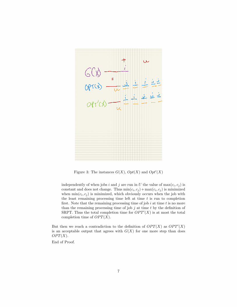
Figure 3: The instances G(X), Opt(X) and Opt′(X)

independently of when jobs i and j are run in U the value of max(ci, cj) isconstant and does not change. Thus min(ci, cj)+max(ci, cj) is minimizedwhen min(ci, cj) is minimized, which obviously occurs when the job withthe least remaining processing time left at time t is run to completionfirst. Note that the remaining processing time of job i at time t is no morethan the remaining processing time of job j at time t by the definition ofSRPT. Thus the total completion time for OPT ′(X) is at most the totalcompletion time of OPT (X).

But then we reach a contradiction to the definition of OPT (X) as OPT ′(X)is an acceptable output that agrees with G(X) for one more step than doesOPT (X).

End of Proof.

7

9 Kruskal’s Minimum Spanning Tree Algorithm

We show that the standard greedy algorithm that considers the jobs from short-est to longest is optimal. See section 4.1.2 from the text.

Lemma: If Kruskal’s algorithm does not included an edge e = (x, y) then at thetime that the algorithm considered e, there was already a path from x to y inthe algorithm’s partial solution.

Theorem: Kruskal’s algorithm is correct.

Proof: We use an exchange argument. Let K be a nonoptimal spanning treeconstructed by Kruskal’s algorithm on some input, and let O be an optimal treethat agrees with the algorithms choices the longest (as we following the choicesmade by Kruskal’s algorithm). Consider the edge e on which they first disagree.We first claim that e ∈ K. Otherwise, by the lemma there was previously a pathbetween the endpoints of e in the K, and since optimal and Kruskal’s algorithmhave agreed to date, O could not include e, which is a contradiction to the factthat O and K disagree on e. Hence, it must be the case that e ∈ K and e /∈ O.

Figure 4: The instances G(X), Opt(X) and Opt′(X)

8

Let x and y be the endpoints of e. Let C = x = z1, z2, . . . , zk be the unique cyclein O ∪ {e}. We now claim that there must be an edge (zp, zp+1)inC − {e} withweight not smaller than e’s weight. To reach a contradiction assume otherwise,that is, that each edge (zi, zi+1 have weight less than the weight of (x, y). Butthen Kruskal’s considered each (zi, zi+1 before (x, y), and by the choice of (x, y)as being the first point of disagreement, each (zi, zi+1) must be in K. Butthis is then a contradiction to K being feasible (obviously Kruskal’s algorithmproduces a feasible solution).

We then let O′ = O+e−(zp, zp+1). Clearly O′ agrees with K longer than O does(note that since the weight of (zp, zp+1) is greater than weight of e, Kruskal’sconsiders (zp, zp+1) after e) and O′ has weight no larger than O’s weight (andhence O′ is still optimal) since the weight of edge (zp, zp+1) is not smaller thanthe weight of e.

EndProof

10 Huffman’s Algorithm

We consider the following problem.

Input: Positive weights p1, . . . , pn

Output: A binary tree with n leaves and a permutaton s on {1, . . . , n} thatminimizes

∑ni=1 ps(i)di, where di is the depth of the ith leaf.

Huffman’s algorithm picks the two smallest weights, say pi and pj , and givesthen a common parent in the tree. The algorithm then replaces pi and pj bya single number pi + pj and recurses. Hence, every node in the final tree islabel with a probability. The probability of each internal node is the sum of theprobabilities of its children.

Lemma: Every leaf in the optimal tree has a sibling.

Proof: Otherwise you could move the leaf up one, decreasing it’s depth andcontradicting optimality.

Theorem: Huffman’s algorithm is correct.

Proof: We use an exchange argument. Let consider the first time where theoptimal solution O differs from the tree H produced by Huffman’s algorithm.Let pi and pj be the siblings that Huffman’s algorithm creates at this time.Hence, pi and pj are not siblings in O. Let pa be sibling of pi in O, and pb bethe sibling of pj in O. Assume without loss of generality that di = da ≤ db = dj .Let s = db − da. Then let O′ be equal to O with the subtrees rooted at pi andpb swapped. The net change in the average depth is kpi − kpb.

Hence in order to show that the average depth does not increase and that O′

is still optimal, we need to show that pi ≤ pb. Assume to reach a contradictionthat indeed it is the case that pb < pi. Then Huffman’s considered pb before itpaired pi and pj . Hence pa’s partner in H is not pi. This contradicts the choice

9

of pi and pj as being the first point where they differ.

Using similar arguments it also follows that pj ≤ pb, pi ≤ pb, and pj ≤ pa.Hence, O′ agrees with H for one more step than O did (note that O and Hcould no.

EndProof.

10