1 binary choice models: logit analysis the linear probability model may make the nonsense...

1

BINARY CHOICE MODELS: LOGIT ANALYSIS

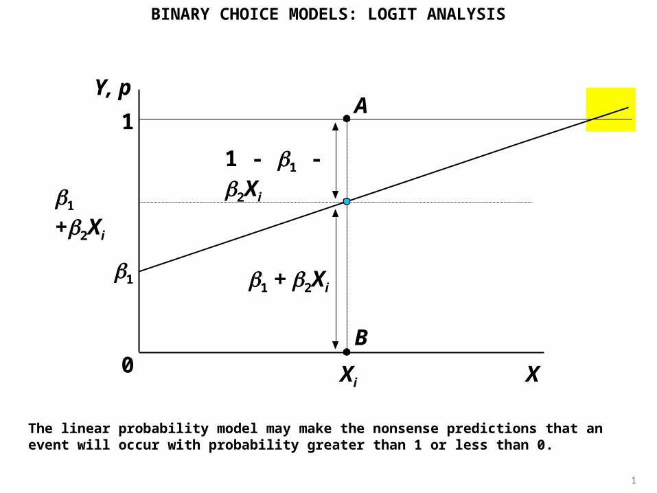
The linear probability model may make the nonsense predictions that an event will occur with probability greater than 1 or less than 0.

XXi

1

0

1 +2Xi

Y, p

1

A

1 - 1 - 2Xi

B

1 + 2Xi

2

0.00

0.25

0.50

0.75

1.00

-8 -6 -4 -2 0 2 4 6 Z

ZeZFp

1

1)(

)(ZF

XZ 21

The usual way of avoiding this problem is to hypothesize that the probability is a sigmoid (S-shaped) function of Z, F(Z), where Z is a function of the explanatory variables.


3

0.00

0.25

0.50

0.75

1.00

-8 -6 -4 -2 0 2 4 6

Several mathematical functions are sigmoid in character. One is the logistic function shown here. As Z goes to infinity, e-Z goes to 0 and p goes to 1 (but cannot exceed 1). As Z goes to minus infinity, e-Z goes to infinity and p goes to 0 (but cannot be below 0).


XZ 21

)(ZFZe

ZFp

11

)(

Z

4

0.00

0.25

0.50

0.75

1.00

-8 -6 -4 -2 0 2 4 6

The model implies that, for values of Z less than -2, the probability of the event occurring is low and insensitive to variations in Z. Likewise, for values greater than 2, the probability is high and insensitive to variations in Z.


XZ 21

)(ZFZe

ZFp

11

)(

Z

5

To obtain an expression for the sensitivity, we differentiate F(Z) with respect to Z. The box gives the general rule for differentiating a quotient and applies it to F(Z).


VU

Y

2VdZdV

UdZdU

V

dZdY

2

2

)1(

)1()(10)1(

Z

Z

Z

ZZ

ee

eee

dZdp

01 dZdU

U

Z

Z

edZdV

eV

)1(

ZeZFp

1

1)(

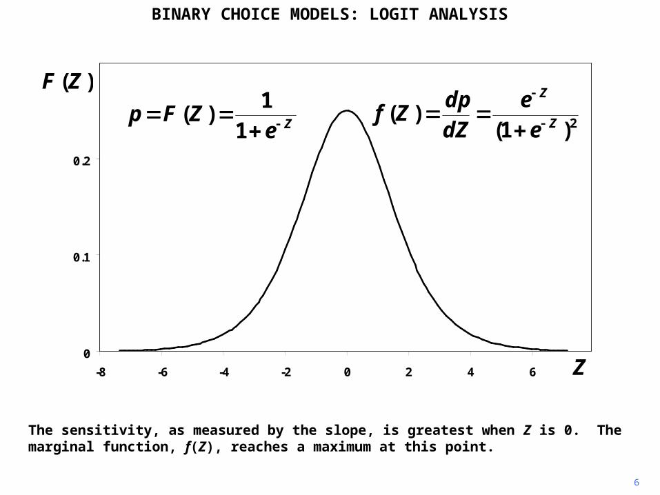
6

0

0.1

0.2

-8 -6 -4 -2 0 2 4 6

2)1()( Z

Z

ee

dZdp

Zf


The sensitivity, as measured by the slope, is greatest when Z is 0. The marginal function, f(Z), reaches a maximum at this point.

ZeZFp

1

1)(

)(ZF

Z

7

0.00

0.25

0.50

0.75

1.00

-8 -6 -4 -2 0 2 4 6

For a nonlinear model of this kind, maximum likelihood estimation is much superior to the use of the least squares principle for estimating the parameters. More details concerning its application are given at the end of this sequence.


ZeZFp

1

1)(

)(ZF

XZ 21

Z

8

0.00

0.25

0.50

0.75

1.00

-8 -6 -4 -2 0 2 4 6

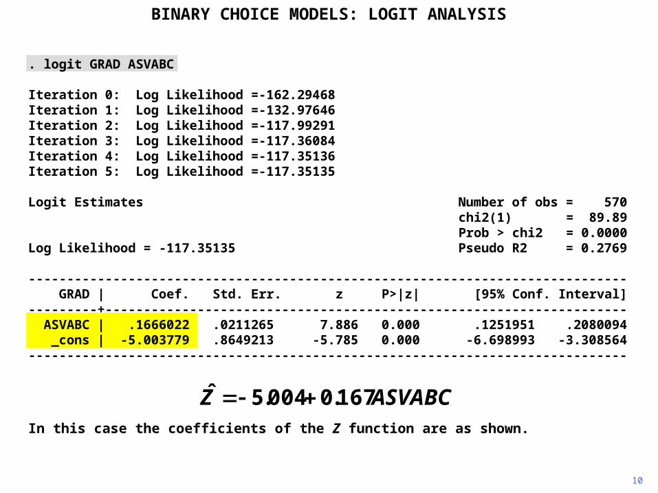
We will apply this model to the graduating from high school example described in the linear probability model sequence. We will begin by assuming that ASVABC is the only relevant explanatory variable, so Z is a simple function of it.


ZeZFp

1

1)(

)(ZF

ASVABCZ 21

Z

. logit GRAD ASVABC

Iteration 0: Log Likelihood =-162.29468Iteration 1: Log Likelihood =-132.97646Iteration 2: Log Likelihood =-117.99291Iteration 3: Log Likelihood =-117.36084Iteration 4: Log Likelihood =-117.35136Iteration 5: Log Likelihood =-117.35135

Logit Estimates Number of obs = 570 chi2(1) = 89.89 Prob > chi2 = 0.0000Log Likelihood = -117.35135 Pseudo R2 = 0.2769

------------------------------------------------------------------------------ grad | Coef. Std. Err. z P>|z| [95% Conf. Interval]---------+-------------------------------------------------------------------- asvabc | .1666022 .0211265 7.886 0.000 .1251951 .2080094 _cons | -5.003779 .8649213 -5.785 0.000 -6.698993 -3.308564------------------------------------------------------------------------------


9

The Stata command is logit, followed by the outcome variable and the explanatory variable(s). Maximum likelihood estimation is an iterative process, so the first part of the output will be like that shown.

. logit GRAD ASVABC



------------------------------------------------------------------------------ GRAD | Coef. Std. Err. z P>|z| [95% Conf. Interval]---------+-------------------------------------------------------------------- ASVABC | .1666022 .0211265 7.886 0.000 .1251951 .2080094 _cons | -5.003779 .8649213 -5.785 0.000 -6.698993 -3.308564------------------------------------------------------------------------------

10

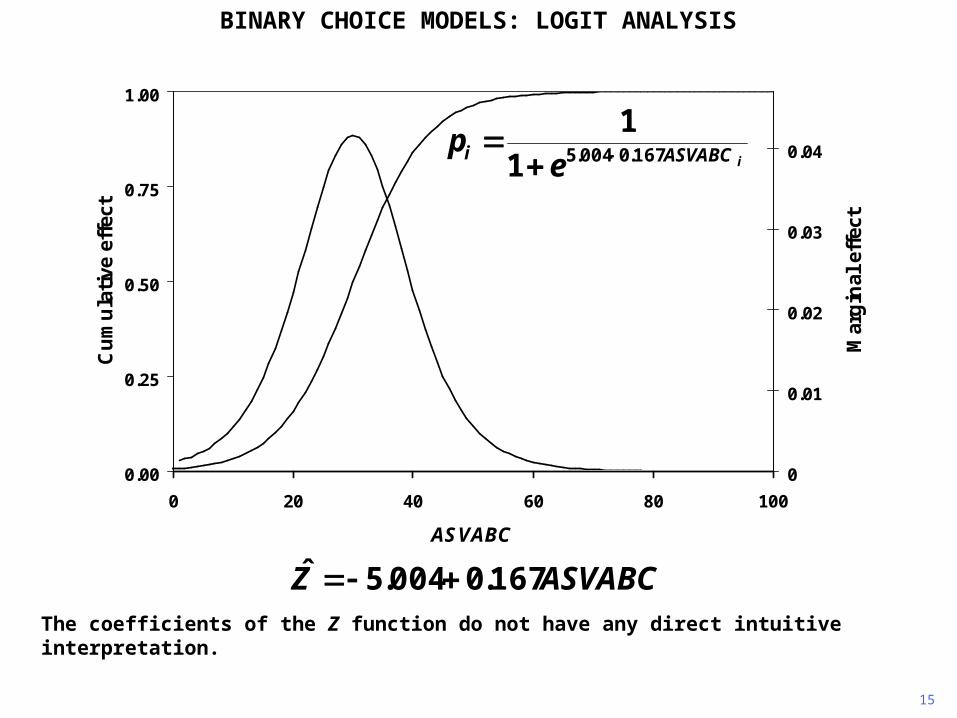
In this case the coefficients of the Z function are as shown.


ASVABCZ 167.0004.5ˆ

11

iASVABCi ep 167.0004.51

1

Since there is only one explanatory variable, we can draw the probability function and marginal effect function as functions of ASVABC.



0.00

0.25

0.50

0.75

1.00

0 20 40 60 80 100

ASVABC

Cu

mu

lati

ve e

ffec

t

0

0.01

0.02

0.03

0.04

Mar

gin

al e

ffec

t


1



0.00

0.25

0.50

0.75

1.00

0 20 40 60 80 100

ASVABC

Cu

mu

lati

ve e

ffec

t

0

0.01

0.02

0.03

0.04

Mar

gin

al e

ffec

t

12

We see that ASVABC has its greatest effect on graduating when it is in the range 20-40, that is, in the lower ability range. Any individual with a score above the average (50) is almost certain to graduate.

13

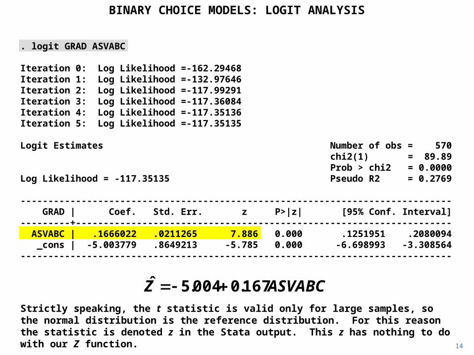
The t statistic indicates that the effect of variations in ASVABC on the probability of graduating from high school is highly significant.



. logit GRAD ASVABC






. logit GRAD ASVABC




14

Strictly speaking, the t statistic is valid only for large samples, so the normal distribution is the reference distribution. For this reason the statistic is denoted z in the Stata output. This z has nothing to do with our Z function.


1



0.00

0.25

0.50

0.75

1.00

0 20 40 60 80 100

ASVABC

Cu

mu

lati

ve e

ffec

t

0

0.01

0.02

0.03

0.04

Mar

gin

al e

ffec

t

15

The coefficients of the Z function do not have any direct intuitive interpretation.

16

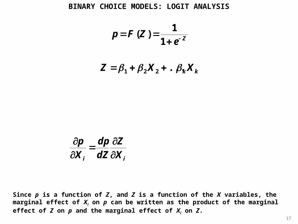
However, we can use them to quantify the marginal effect of a change in ASVABC on the probability of graduating. We will do this theoretically for the general case where Z is a function of several explanatory variables.


kk XXZ ...221

ZeZFp

1

1)(

17

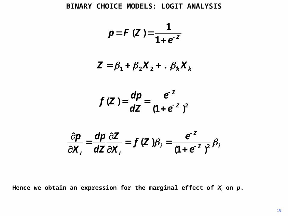
Since p is a function of Z, and Z is a function of the X variables, the marginal effect of Xi on p can be written as the product of the marginal effect of Z on p and the marginal effect of Xi on Z.


iZ

Z

iii e

eZf

XZ

dZdp

Xp 2)1(

)(

kk XXZ ...221

ZeZFp

1

1)(

18

We have already derived an expression for dp/dZ. The marginal effect of Xi on Z is given by

its coefficient.


iZ

Z

iii e

eZf

XZ

dZdp

Xp 2)1(

)(

2)1()( Z

Z

ee

dZdp

Zf

kk XXZ ...221

ZeZFp

1

1)(

19

Hence we obtain an expression for the marginal effect of Xi on p.


iZ

Z

iii e

eZf

XZ

dZdp

Xp 2)1(

)(

kk XXZ ...221

ZeZFp

1

1)(

2)1()( Z

Z

ee

dZdp

Zf

20

kk XXZ ...221

ZeZFp

1

1)(

iZ

Z

iii e

eZf

XZ

dZdp

Xp 2)1(

)(

2)1()( Z

Z

ee

dZdp

Zf

The marginal effect is not constant because it depends on the value of Z, which in turn depends on the values of the explanatory variables. A common procedure is to evaluate it for the sample means of the explanatory variables.


21

The sample mean of ASVABC was 50.15.


. sum GRAD ASVABC

Variable | Obs Mean Std. Dev. Min Max---------+----------------------------------------------------- GRAD | 570 .9175439 .2753 0 1 ASVABC | 570 50.15088 9.214589 22 65



. sum GRAD ASVABC




22

When evaluated at the mean, Z is equal to 3.371.


371.315.50167.0004.521 XZ

23

e-Z is 0.034. Hence f(Z) is 0.032.


371.315.50167.0004.521 XZ

034.0371.3 ee Z

032.0)034.01(

034.0)1(

)( 22

Z

Z

ee

dZdp

Zf

. sum GRAD ASVABC


24

The marginal effect, evaluated at the mean, is therefore 0.005. This implies that a one point increase in ASVABC would increase the probability of graduating from high school by 0.5 percent.


032.0)034.01(

034.0)1(

)( 22

Z

Z

ee

dZdp

Zf

005.0167.0032.0)(

iii

ZfXZ

dZdp

Xp

. sum GRAD ASVABC


371.315.50167.0004.521 XZ

034.0371.3 ee Z

25

In this example, the marginal effect at the mean of ASVABC is very low. The reason is that anyone with an average score is very likely to graduate anyway. So an increase in the score has little effect.


50.15

0.00

0.25

0.50

0.75

1.00

0 20 40 60 80 100

ASVABC

Cu

mu

lati

ve e

ffec

t

0

0.01

0.02

0.03

0.04

Mar

gin

al e

ffec

t

. sum COLLEGE ASVABC

Variable | Obs Mean Std. Dev. Min Max---------+----------------------------------------------------- COLLEGE | 570 .4964912 .5004269 0 1 ASVABC | 570 50.15088 9.214589 22 65

26

To show that the marginal effect varies, we will also calculate it for ASVABC equal to 30. A one point increase in ASVABC then increases the probability by 4.2 percent.


994.0006.0 ee Z

250.0)994.01(

994.0)1(

)( 22

Z

Z

ee

dZdp

Zf

042.0167.0250.0)(

iii

ZfXZ

dZdp

Xp

006.030167.0004.521 XZ

27

An individual with a score of 30 has only a 50 percent probability of graduating, and an increase in the score has a relatively large impact.


0.89 0.042

0.00

0.25

0.50

0.75

1.00

0 20 40 60 80 100

ASVABC

Cu

mu

lati

ve e

ffec

t

0

0.01

0.02

0.03

0.04

Mar

gin

al e

ffec

t

30

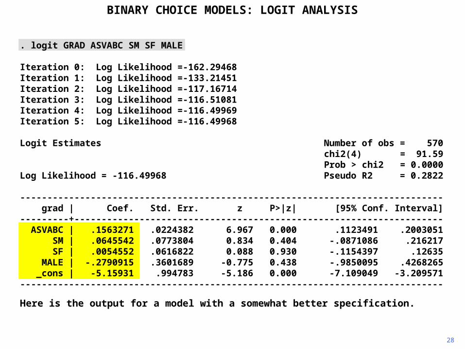
. logit GRAD ASVABC SM SF MALE



------------------------------------------------------------------------------ grad | Coef. Std. Err. z P>|z| [95% Conf. Interval]---------+-------------------------------------------------------------------- ASVABC | .1563271 .0224382 6.967 0.000 .1123491 .2003051 SM | .0645542 .0773804 0.834 0.404 -.0871086 .216217 SF | .0054552 .0616822 0.088 0.930 -.1154397 .12635 MALE | -.2790915 .3601689 -0.775 0.438 -.9850095 .4268265 _cons | -5.15931 .994783 -5.186 0.000 -7.109049 -3.209571------------------------------------------------------------------------------

28

Here is the output for a model with a somewhat better specification.


. sum GRAD ASVABC SM SF MALE

Variable | Obs Mean Std. Dev. Min Max---------+----------------------------------------------------- GRAD | 570 .9175439 .2753 0 1 ASVABC | 570 50.15088 9.214589 22 65 SM | 570 11.65263 2.561449 0 20 SF | 570 11.81754 3.533178 0 20 MALE | 570 .5701754 .4954857 0 1

29

We will estimate the marginal effects, putting all the explanatory variables equal to their sample means.


Logit: Marginal Effects

mean b product f(Z) f(Z)b

ASVABC 50.15 0.156 7.839 0.033 0.005

SM 11.65 0.065 0.753 0.033 0.002

SF 11.82 0.006 0.065 0.033 0.000

MALE 0.57 -0.279 -0.159 0.033 -0.009

Constant 1.00 -5.159 -5.159

Total 3.338

30


The first step is to calculate Z, when the X variables are equal to their sample means.

338.3

...221

kk XXZ



ASVABC 50.15 0.156 7.839 0.033 0.005

SM 11.65 0.065 0.753 0.033 0.002

SF 11.82 0.006 0.065 0.033 0.000

MALE 0.57 -0.279 -0.159 0.033 -0.009

Constant 1.00 -5.159 -5.159

Total 3.338

31


We then calculate f(Z).

036.338.3 ee Z

033.0)1(

)( 2

Z

Z

ee

Zf



ASVABC 50.15 0.156 7.839 0.033 0.005

SM 11.65 0.065 0.753 0.033 0.002

SF 11.82 0.006 0.065 0.033 0.000

MALE 0.57 -0.279 -0.159 0.033 -0.009

Constant 1.00 -5.159 -5.159

Total -3.338

32

The estimated marginal effects are f(Z) multiplied by the respective coefficients. We see that the effect of ASVABC is about the same as before. Every extra year of schooling of the mother increases the probability of graduating by 0.2 percent.


iii

ZfXZ

dZdp

Xp )(



ASVABC 50.15 0.156 7.839 0.033 0.005

SM 11.65 0.065 0.753 0.033 0.002

SF 11.82 0.006 0.065 0.033 0.000

MALE 0.57 -0.279 -0.159 0.033 -0.009

Constant 1.00 -5.159 -5.159

Total -3.338

33


iii

ZfXZ

dZdp

Xp )(

Father's schooling has no discernible effect. Males have 0.9 percent lower probability of graduating than females. These effects would all have been larger if they had been evaluated at a lower ASVABC score.

Individuals who graduated: outcome probability is

34

This sequence will conclude with an outline explanation of how the model is fitted using maximum likelihood estimation.


iASVABCe 211

1

ASVABCZ 21

ASVABC

Z

e

eZFp

211

11

1)(

35

In the case of an individual who graduated, the probability of that outcome is F(Z). We will give subscripts 1, ..., s to the individuals who graduated.


iASVABCe 211

1

ASVABCZ 21

ASVABC

Z

e

eZFp

211

11

1)(


36

In the case of an individual who did not graduate, the probability of that outcome is 1 - F(Z). We will give subscripts s+1, ..., n to these individuals.


iASVABCe 211

1

iASVABCe 211

11

Maximize F(Z1) x ... x F(Zs) x [1 - F(Zs+1)] x ... x [1 - F(Zn)]


Individuals did not graduate: outcome probability is

Maximize F(Z1) x ... x F(Zs) x [1 - F(Zs+1)] x ... x [1 - F(Zn)]

Did graduate Did not graduate

37

We choose b1 and b2 so as to maximize the joint probability of the outcomes, that is, F(Z1) x ... x F(Zs) x [1 - F(Zs+1)] x ... x [1 - F(Zn)]. There are no mathematical formulae for b1 and b2. They have to be determined iteratively by a trial-and-error process.


iASVABCe 211

1 iASVABCe 211

11

ns

s

ASVABCbbASVABCbb

ASVABCbbASVABCbb

ee

ee

21121

21121

1

11...

1

11

1

1...

1

1

1 binary choice models: logit analysis the linear probability model may make the nonsense...

Documents