1 . bounded suboptimal search: weighted a*

CS188 Fall 2018 Review: Final Preparation

1 . Bounded suboptimal search: weighted A*In this class you met A*, an algorithm for informed search guaranteed to return an optimal solution when given anadmissible heuristic. Often in practical applications it is too expensive to find an optimal solution, so instead wesearch for good suboptimal solutions.

Weighted A* is a variant of A* commonly used for suboptimal search. Weighted A* is exactly the same as A* butwhere the f-value is computed differently:

f(n) = g(n) + ε h(n)

where ε ≥ 1 is a parameter given to the algorithm. In general, the larger the value of ε, the faster the search is, andthe higher cost of the goal found.

Pseudocode for weighted A* tree search is given below. NOTE: The only differences from the A* tree searchpseudocode presented in the lectures are: (1) fringe is assumed to be initialized with the start node before thisfunction is called (this will be important later), and (2) now Insert takes ε as a parameter so it can compute thecorrect f -value of the node.

1: function Weighted-A*-Tree-Search(problem, fringe, ε)2: loop do3: if fringe is empty then return failure4: node← Remove-Front(fringe)5: if Goal-Test(problem, State[node]) then return node6: for child-node in child-nodes do7: fringe← Insert(child-node, fringe, ε)

(a) We’ll first examine how weighted A* works on the following graph:

S"h"="8"

A"h"="1"

B"h"="7"

G1"h"="0"

C"h"="1"

D"h"="2"

5

10"

6" 1"

1"

2"6"

G3"h"="0"

G2"h"="0"

Execute weighted A* on the above graph with ε = 2, completing the following table. To save time, you canoptionally just write the nodes added to the fringe, with their g and f values.

node Goal? fringe- - {S : g = 0, f = 16}S No {S → A : g = 5, f = 7;S → B : g = 6, f = 20}S → A No {S → A→ G1 : g = 15, f = 15;S → B : g = 6, f = 20}S → A→ G1 Yes -

1

(b) After running weighted A* with weight ε ≥ 1 a goal node G is found, of cost g(G). Let C∗ be the optimalsolution cost, and suppose the heuristic is admissible. Select the strongest bound below that holds, and providea proof.

g(G) ≤ εC∗ © g(G) ≤ C∗ + ε © g(G) ≤ C∗ + 2ε © g(G) ≤ 2ε C∗ © g(G) ≤ ε2 C∗

Proof: (Partial credit for reasonable proof sketches.)

When weighted A* terminates, an ancestor n of the optimal goal G∗ is on the fringe. Since G was expandedbefore n, we have f(G) ≤ f(n). As a result:

g(G) = f(G) ≤ f(n) = g(n) + εh(n) ≤ ε (g(n) + h(n)) ≤ εC∗

If you’re confused about whether this all comes from, rembmer that f(n) = g(n) + εh(n) comes from theproblem statement and the inequality g(n) + εh(n) ≤ ε(g(n) + h(n)) is true by algebra.Since we know that g(n) is non-negative, it must be true that g(n) + εh(n) <= ε(g(n) + h(n)). This is acommon technique used when trying to prove/find a bound.

(c) Weighted A* includes a number of other algorithms as special cases. For each of the following, name thecorresponding algorithm.

(i) ε = 1.

Algorithm: A*

(ii) ε = 0.

Algorithm: UCS

(iii) ε→∞ (i.e., as ε becomes arbitrarily large).

Algorithm: Greedy search

2

(d) Here is the same graph again:

S"h"="8"

A"h"="1"

B"h"="7"

G1"h"="0"

C"h"="1"

D"h"="2"

5

10"

6" 1"

1"

2"6"

G3"h"="0"

G2"h"="0"

(i) Execute weighted A* on the above graph with ε = 1, completing the following table as in part (a):

node Goal? fringe- - {S : g = 0, f = 8}

S No {S → A : g = 5, f = 6;S → B : g = 6, f = 13}

S → A No {S → B : g = 6, f = 13;S → A→ G1 : g = 15, f = 15}

S → B No {S → B → C : g = 7, f = 8;S → A→ G1 : g = 15, f = 15}

S → B → C No {S → B → C → D : g = 8, f = 10;S → B → C → G2 : g = 13, f = 13;S → A→ G1 : g = 15, f = 15}

S → B → C → D No {S → B → C → D → G3 : g = 10, f = 10;S → B → C → G2 : g = 13, f = 13;S → A→ G1 : g = 15, f = 15}

S → B → C → D → G3 Yes -

(ii) You’ll notice that weighted A* with ε = 1 repeats computations performed when run with ε = 2. Is therea way to reuse the computations from the ε = 2 search by starting the ε = 1 search with a different fringe?Let F denote the set that consists of both (i) all nodes the fringe the ε = 2 search ended with, and (ii)the goal node G it selected. Give a brief justification for your answer.

© Use F as new starting fringe© Use F with goal G removed as new starting fringe Use F as new starting fringe, updating the f -values to account for the new ε© Use F with goal G removed as new starting fringe, updating the f -values to account for the new ε© Initialize the new starting fringe to all nodes visited in previous search© Initialize the new starting fringe to all nodes visited in previous search, updating the f -values to ac-count for the new ε© It is not possible to reuse computations, initialize the new starting fringe as usual

Justification:

We have to include G in the fringe as it might still be optimal (e.g. if it is the only goal). We don’t haveto update the g-values, but we do have the update the f -values to reflect the new value of ε. With thesemodifications, it is valid to continue searching as the state of the fringe is as if A* with the new ε wasrun, but with some extraneous node expansions.

3

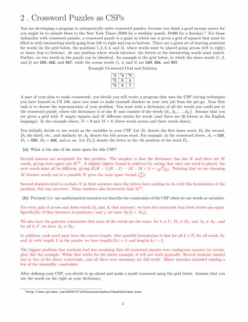
2 . Crossword Puzzles as CSPsYou are developing a program to automatically solve crossword puzzles, because you think a good income source foryou might be to submit them to the New York Times ($200 for a weekday puzzle, $1000 for a Sunday).1 For thoseunfamiliar with crossword puzzles, a crossword puzzle is a game in which one is given a grid of squares that must befilled in with intersecting words going from left to right and top to bottom. There are a given set of starting positionsfor words (in the grid below, the positions 1, 2, 3, 4, and 5), where words must be placed going across (left to right)or down (top to bottom). At any position where words intersect, the letters in the intersecting words must match.Further, no two words in the puzzle can be identical. An example is the grid below, in which the down words (1, 2,and 3) are DEN, ARE, and MAT, while the across words (1, 4, and 5) are DAM, ERA, and NET.

Example Crossword Grid and Solution

1D 2A 3M4E R A5N E T

A part of your plan to make crosswords, you decide you will create a program that uses the CSP solving techniquesyou have learned in CS 188, since you want to make yourself obsolete at your own job from the get-go. Your firsttask is to choose the representation of your problem. You start with a dictionary of all the words you could put inthe crossword puzzle, where the dictionary is of size K and consists of the words {d1, d2, . . . , dK}. Assume that youare given a grid with N empty squares and M different entries for words (and there are 26 letters in the Englishlanguage). In the example above, N = 9 and M = 6 (three words across and three words down).

You initially decide to use words as the variables in your CSP. Let D1 denote the first down word, D2 the second,D3 the third, etc., and similarly let Ak denote the kth across word. For example, in the crossword above, A1 = DAM,D1 = DEN, D2 = ARE, and so on. Let D1[i] denote the letter in the ith position of the word D1.

(a) What is the size of the state space for this CSP?

Several answers are acceptable for this problem. The simplest is that the dictionary has size K and there are Mwords, giving state space size KM . A slightly tighter bound is achieved by noting that once one word is placed, thenext words must all be different, giving K(K − 1)(K − 2) · · · (K −M + 1) = K!

(K−M)! . Noticing that we are choosing

M distinct words out of a possible K gives the state space bound(KM

).

Several students tried to include N in their answers; since the letters have nothing to do with this formulation of theproblem, this was incorrect. Many students also incorrectly had MK .

(b) Precisely (i.e. use mathematical notation to) describe the constraints of the CSP when we use words as variables.

For every pair of across and down words Dk and Al that intersect, we have the constraint that their letters are equal.Specifically, if they intersect in positions i and j, we have Dk[i] = Al[j].

We also have the pairwise constraints that none of the words are the same: for k 6= k′, Dk 6= Dk′ and Ak 6= Ak′ , andfor all k, k′, we have Ak 6= Dk′ .

In addition, each word must have the correct length. One possible formulation is that for all L ∈ N, for all words Dk

and Al with length L in the puzzle, we have length(Dk) = L and length(Al) = L.

The biggest problem that students had was assuming that all crossword puzzles were contiguous squares (or rectan-gles) like the example. While that works for the above example, it will not work generally. Several students missedone or two of the above constraints, and all three were necessary for full credit. Minor mistakes included missing afew of the inequality constraints.

After defining your CSP, you decide to go ahead and make a small crossword using the grid below. Assume that youuse the words on the right as your dictionary.

1http://www.nytimes.com/2009/07/19/business/media/19askthetimes.html

4

Crossword Grid Dictionary Words1 2 3 4

5

6

7

ARCS, BLAM, BEAR, BLOGS, LARD, LARP,

GAME, GAMUT, GRAMS, GPS, MDS, ORCS, WARBLER

(c) Enforce all unary constraints by crossing out values in the table below.

D1 ARCS BLAM BEAR BLOGS LARD LARP GPS MDS GAME GAMUT GRAMS ORCS WARBLER




A1 ARCS BLAM BEAR BLOGS LARD LARP GPS MDS GAME GAMUT GRAMS ORCS WARBLER




(d) Assume that in backtracking search, we assign A1 to be GRAMS. Enforce unary constraints, and in addition,cross out all the values eliminated by forward checking against A1 as a result of this assignment.









(e) Now let’s consider how much arc consistency can prune the domains for this problem, even when no assignmentshave been made yet. I.e., assume no variables have been assigned yet, enforce unary constraints first, and thenenforce arc consistency by crossing out values in the table below.









The common mistake in this question was to leave a few blocks of words that students thought could not be eliminated.Probably the most common was to allow both LARD and LARP for D2 and A5. This is incorrect; for D2, no assignmentof A7 is consistent with LARP, and for A5, no assignment of D4 is consistent with LARD.

(f) How many solutions to the crossword puzzle are there? Fill them (or the single solution if there is only one) inbelow.

1B 2L 3O 4G S5L A R P6A R C S7M D S

1 2 3 4

5

6

7

1 2 3 4

5

6

7

There is one solution (above)

Your friend suggests using letters as variables instead of words, thinking that sabotaging you will be funny. Startingfrom the top-left corner and going left-to-right then top-to-bottom, let X1 be the first letter, X2 be the second, X3

5

the third, etc. In the very first example, X1 = D, X2 = A, and so on.

(g) What is the size of the state space for this formulation of the CSP?

26N . There are 26 letters and N possible positions.

(h) Assume that in your implementation of backtracking search, you use the least constraining value heuristic.Assume that X1 is the first variable you choose to instantiate. For the crossword puzzle used in parts (c)-(f),what letter(s) might your search assign to X1?

We realized that this question was too vague to be answered correctly, so we gave everyone 2 points for the problem.The least constraining value heuristic, once a variable has been chosen, assigns the value that according to somemetric (chosen by the implementer of the heuristic) leaves the domains of the remaining variables most open. Howone eliminates values from the domains of other variables upon an assignment can impact the choice of the value aswell (whether one uses arc consistency or forward checking).

We now sketch a solution to the problem assuming we use forward checking. Let X1, X2, . . . , X5 be the letters inthe top row of the crossword and X1, X6, X7, X8 be the first column down. Upon assigning X1 = G, the possibledomains for the remaining letters are

X2 ∈ {A, R}, X3 ∈ {M, A}, X4 ∈ {U, M}, X5 ∈ {T, S}, X6 ∈ {A}, X7 ∈ {M}, X8 ∈ {E}.

Upon assigning X1 = B, the possible domains remaining are

X2 ∈ {L}, X3 ∈ {O}, X4 ∈ {G}, X5 ∈ {S}, X6 ∈ {L, E}, X7 ∈ {A}, X8 ∈ {M, R}.

The remaining variables are unaffected since we are using only forward checking. Now, we see that with the assignmentX1 = G, the minimum size remaining for any domain is 1, while the sum of the sizes remaining domains is 11; forX1 = B, the minimum size is 1, while the sum of the sizes remaining is 9. So depending on whether we use minimumdomain or the sum of the sizes of the remaining domains, the correct solutions are G and B or only G, respectively.

Any choice but X1 = B or X1 = G will eliminate all values for one of the other variables after forward checking.

6

3 . Game TreesThe following problems are to test your knowledge of Game Trees.

(a) Minimax

The first part is based upon the following tree. Upward triangle nodes are maximizer nodes and downward areminimizers. (small squares on edges will be used to mark pruned nodes in part (ii))

5

5

8

�

6

�

7

�

5

�

�

4

9

9

�

2

�

�

10

8

�

10

�

2

�

�

4

3

�

2 4

�

�

6

0

�

5

�

6

�

�

�

(i) Complete the game tree shown above by filling in values on the maximizer and minimizer nodes.

(ii) Indicate which nodes can be pruned by marking the edge above each node that can be pruned (you donot need to mark any edges below pruned nodes). In the case of ties, please prune any nodes that couldnot affect the root node’s value. Fill in the bubble below if no nodes can be pruned.

© No nodes can be pruned

7

(b) Food Dimensions

The following questions are completely unrelated to the above parts.

Pacman is playing a tricky game. There are 4 portals to food dimensions. But, these portals are guarded bya ghost. Furthermore, neither Pacman nor the ghost know for sure how many pellets are behind each portal,though they know what options and probabilities there are for all but the last portal.

Pacman moves first, either moving West or East. After which, the ghost can block 1 of the portals available.

You have the following gametree. The maximizer node is Pacman. The minimizer nodes are ghosts and theportals are chance nodes with the probabilities indicated on the edges to the food. In the event of a tie, theleft action is taken. Assume Pacman and the ghosts play optimally.

64

64

P1

55

25

70

35

66

P2

30

110

70

910

West

65

P3

45

13

75

23

P4

X

12

Y

12

East

(i) Fill in values for the nodes that do not depend on X and Y .

(ii) What conditions must X and Y satisfy for Pacman to move East? What about to definitely reachthe P4? Keep in mind that X and Y denote numbers of food pellets and must be whole numbers:X,Y ∈ {0, 1, 2, 3, . . . }.

To move East: X + Y > 128

To reach P4: X + Y = 129

The first thing to note is that, to pick A over B, value(A) > value(B).Also, the expected value of the parent node of X and Y is X+Y

2 .

=⇒ min(65, X+Y2 ) > 64

=⇒ X+Y2 > 64

So, X + Y > 128 =⇒ value(A) > value(B)

To ensure reaching X or Y , apart from the above, we also have X+Y2 < 65

=⇒ 128 < X + Y < 130So, X,Y ∈ N =⇒ X + Y = 129

8

4 . Discount MDPs

Consider the above gridworld. An agent is currently on grid cell S, and would like to collect the rewards that lie onboth sides of it. If the agent is on a numbered square, its only available action is to Exit, and when it exits it getsreward equal to the number on the square. On any other (non-numbered) square, its available actions are to moveEast and West. Note that North and South are never available actions.

If the agent is in a square with an adjacent square downward, it does not always move successfully: when the agentis in one of these squares and takes a move action, it will only succeed with probability p. With probability 1 − p,the move action will fail and the agent will instead move downwards. If the agent is not in a square with an adjacentspace below, it will always move successfully.

For parts (a) and (b), we are using discount factor γ ∈ [0, 1].

(a) Consider the policy πEast, which is to always move East (right) when possible, and to Exit when that is theonly available action. For each non-numbered state x in the diagram below, fill in V πEast(x) in terms of γ and p.

(b) Consider the policy πWest, which is to always move West (left) when possible, and to Exit when that is theonly available action. For each non-numbered state x in the diagram below, fill in V πWest(x) in terms of γ and p.

9

(c) For what range of values of p in terms of γ is it optimal for the agent to go West (left) from the start state(S)?

We want 5γ2 ≥ 10γ3p2, which we can solve to get:

Range: p ∈ [0, 1√2γ

]

(d) For what range of values of p in terms of γ is πWest the optimal policy?

We need, for each of the four cells, to have the value of that cell under πWest to be at least as large as πEast.Intuitively, the farther east we are, the higher the value of moving east, and the lower the value of moving west(since the discount factor penalizes far-away rewards).Thus, if moving west is the optimal policy, we want to focus our attention on the rightmost cell.At the rightmost cell, in order for moving west to be optimal, then V πEast(s) ≤ V πWest(s), which is 10γp ≤ 5γ4p2,or p ≥ 2

γ3 .

However, since γ ranges from 0 to 1, the right side of this expression ranges from 2 to ∞, which means p (aprobability, and thus bounded by 1) has no valid value.Range: ∅

(e) For what range of values of p in terms of γ is πEast the optimal policy?

We follow the same logic as in the previous part. Specifically, we focus on the leftmost cell, where the conditionfor πEast to be the optimal policy is: 10γ4p2 ≥ 5γ, which simplifies to p ≥ 1√

2γ3. Combined with our bound

on any probability being in the range [0, 1], we get:

Range: p ∈[

1√2γ3

, 1

], which could be an empty set depending on γ.

Recall that in approximate Q-learning, the Q-value is a weighted sum of features: Q(s, a) =∑i wifi(s, a). To

derive a weight update equation, we first defined the loss function L2 = 12 (y −

∑k wkfk(x))2 and found dL2/dwm =

−(y−∑k wkfk(x))fm(x). Our label y in this set up is r+ γmaxaQ(s′, a′). Putting this all together, we derived the

gradient descent update rule for wm as wm ← wm + α (r + γmaxaQ(s′, a′)−Q(s, a)) fm(s, a).

In the following question, you will derive the gradient descent update rule for wm using a different loss function:

L1 =

∣∣∣∣∣y −∑k

wkfk(x)

∣∣∣∣∣(f) Find dL1/dwm. Show work to have a chance at receiving partial credit. Ignore the non-differentiable point.

Note that the derivative of |x| is −1 if x < 0 and 1 if x > 0. So for L1, we have:

dL1

dwm=

{−fm(x) y −

∑k wkfk(x) > 0

fm(x) y −∑k wkfk(x) < 0

(g) Write the gradient descent update rule for wm, using the L1 loss function.

wm ← wm − αdL1/dwm

←

{wm + αfm(x) y −

∑k wkfk(x) > 0

wm − αfm(x) y −∑k wkfk(x) < 0

10

5 . Q-Learning Strikes BackConsider the grid-world given below and Pacman who is trying to learn the optimal policy. If an action results inlanding into one of the shaded states the corresponding reward is awarded during that transition. All shaded statesare terminal states, i.e., the MDP terminates once arrived in a shaded state. The other states have the North, East,South, West actions available, which deterministically move Pacman to the corresponding neighboring state (or havePacman stay in place if the action tries to move out of the grad). Assume the discount factor γ = 0.5 and theQ-learning rate α = 0.5 for all calculations. Pacman starts in state (1, 3).

(a) What is the value of the optimal value function V ∗ at the following states:

V ∗(3, 2) = 100 V ∗(2, 2) = 50 V ∗(1, 3) = 12.5

The optimal values for the states can be found by computing the expected reward for the agent acting optimallyfrom that state onwards. Note that you get a reward when you transition into the shaded states and not out of them.So for example the optimal path starting from (2,2) is to go to the +100 square which has a discounted reward of0 + γ ∗ 100 = 50. For (1,3), going to either of +25 or +100 has the same discounted reward of 12.5.

(b) The agent starts from the top left corner and you are given the following episodes from runs of the agentthrough this grid-world. Each line in an Episode is a tuple containing (s, a, s′, r).

Episode 1 Episode 2 Episode 3(1,3), S, (1,2), 0 (1,3), S, (1,2), 0 (1,3), S, (1,2), 0(1,2), E, (2,2), 0 (1,2), E, (2,2), 0 (1,2), E, (2,2), 0(2,2), S, (2,1), -100 (2,2), E, (3,2), 0 (2,2), E, (3,2), 0

(3,2), N, (3,3), +100 (3,2), S, (3,1), +80

Using Q-Learning updates, what are the following Q-values after the above three episodes:

Q((3,2),N) = 50 Q((1,2),S) = 0 Q((2, 2), E) = 12.5

Q-values obtained by Q-learning updates - Q(s, a)← (1− α)Q(s, a) + α(R(s, a, s′) + γmaxa′ Q(s′, a′)).

(c) Consider a feature based representation of the Q-value function:

Qf (s, a) = w1f1(s) + w2f2(s) + w3f3(a)

f1(s) : The x coordinate of the state f2(s) : The y coordinate of the state

f3(N) = 1, f3(S) = 2, f3(E) = 3, f3(W ) = 4

(i) Given that all wi are initially 0, what are their values after the first episode:

11

w1 = -100 w2 = -100 w3 = -100

Using the approximate Q-learning weight updates: wi ← wi+α[(R(s, a, s′)+γmaxa′ Q(s′, a′))−Q(s, a)]fi(s, a).The only time the reward is non zero in the first episode is when it transitions into the -100 state.

(ii) Assume the weight vector w is equal to (1, 1, 1). What is the action prescribed by the Q-function in state(2, 2) ?

West

The action prescribed at (2,2) is maxaQ((2, 2), a) where Q(s, a) is computed using the feature represen-tation. In this case, the Q-value for West is maximum (2 + 2 + 4 = 8).

12

6 . Probability(a) Consider the random variables A,B, and C. Circle all of the following equalities that are always true, if any.

1. P(A,B) = P(A)P(B)−P(A|B)

2. P(A,B) = P(A)P(B)

3. P(A,B) = P(A|B)P(B) + P(B|A)P(A)

4. P(A) =∑b∈B P(A|B = b)P(B = b)

5. P(A,C) =∑b∈B P(A|B = b)P(C|B = b)P(B = b)

6. P(A,B,C) = P(C|A)P(B|C,A)P(A)

Now assume that A and B both can take on only the values true and false (A ∈ {true, false} and B ∈ {true, false}).You are given the following quantities:

P(A = true) = 12

P(B = true | A = true) = 1P(B = true) = 3

4

(b) What is P(B = true | A = false)?

Many people got lost trying to directly apply Bayes’ rule. The simplest way to solve this is to realize that

P(B = true) = P(B = true | A = true)P(A = true) + P(B = true | A = false)P(A = false).

Using this fact, you can solve for P(B = true | A = false):

(1)

(1

2

)+ P(B = true | A = false)

(1

2

)=

3

4

=⇒ P(B = true | A = false)

(1

2

)=

1

4

=⇒ P(B = true | A = false) =1

2

Therefore P(B = true | A = false) = 12 .

13

7 . Bayes’ Nets: Short Questions(a) Bayes’ Nets: Conditional Independence

Based only on the structure of the (new) Bayes’ Net given below, circle whether the following conditionalindependence assertions are guaranteed to be true, guaranteed to be false, or cannot be determined by thestructure alone.Note: The ordering of the three answer columns might have been switched relative to previousexams!

1 A ⊥⊥ C Guaranteed false Cannot be determined Guaranteed true

2 A ⊥⊥ C | E Guaranteed false Cannot be determined Guaranteed true

3 A ⊥⊥ C | G Guaranteed false Cannot be determined Guaranteed true

4 A ⊥⊥ K Guaranteed false Cannot be determined Guaranteed true

5 A ⊥⊥ G | D,E, F Guaranteed false Cannot be determined Guaranteed true

6 A ⊥⊥ B | D,E, F Guaranteed false Cannot be determined Guaranteed true

7 A ⊥⊥ C | D,F,K Guaranteed false Cannot be determined Guaranteed true

8 A ⊥⊥ G | D Guaranteed false Cannot be determined Guaranteed true

14

(b) Bayes’ Nets: Elimination of a Single Variable

Assume we are running variable elimination, and we currently have the following three factors:

A B f1(A,B)+a +b 0.1+a −b 0.5−a +b 0.2−a −b 0.5

A C D f2(A,C,D)+a +c +d 0.2+a +c −d 0.1+a −c +d 0.5+a −c −d 0.1−a +c +d 0.5−a +c −d 0.2−a −c +d 0.5−a −c −d 0.2

B D f3(B,D)+b +d 0.2+b −d 0.2−b +d 0.5−b −d 0.1

The next step in the variable elimination is to eliminate B.

(i) Which factors will participate in the elimination process of B? f1, f3

(ii) Perform the join over the factors that participate in the elimination of B. Your answer should be a tablesimilar to the tables above, it is your job to figure out which variables participate and what the numericalentries are.A B D f ′4(A,B,D)

+a +b +d 0.1*0.2 = 0.02+a +b −d 0.1*0.2 = 0.02+a −b +d 0.5*0.5 = 0.25+a −b −d 0.5*0.1 = 0.05−a +b +d 0.2*0.2 = 0.04−a +b −d 0.2*0.2 = 0.04−a −b +d 0.5*0.5 = 0.25−a −b −d 0.5*0.1 = 0.05

(iii) Perform the summation over B for the factor you obtained from the join. Your answer should be a tablesimilar to the tables above, it is your job to figure out which variables participate and what the numericalentries are.A D f4(A,D)

+a +d 0.02+ 0.25 = 0.27+a −d 0.02 + 0.05 = 0.07−a +d 0.04 + 0.25 = 0.29−a −d 0.04 + 0.05 = 0.09

15

(c) Elimination Sequence

For the Bayes’ net shown below, consider the query P (A|H = +h), and the variable elimination orderingB,E,C, F,D.

(i) In the table below fill in the factor generated at each step — we did the first row for you.

A B C

D E F

HVariable Factor Current

Eliminated Generated Factors

(no variable eliminated yet) (no factor generated) P (A), P (B), P (C), P (D|A), P (E|B), P (F |C), P (+h|D,E, F )

B f1(E) P (A), P (C), P (D|A), P (F |C), P (+h|D,E, F ), f1(E)

E f2(+h,D, F ) P (A), P (C), P (D|A), P (F |C), f2(+h,D, F )

C f3(F ) P (A), P (D|A), f2(+h,D, F ), f3(F )

F f4(+h,D) P (A), P (D|A), f4(+h,D)

D f5(+h,A) P (A), f5(+h,A)

(ii) Which is the largest factor generated? Assuming all variables have binary-valued domains, how manyentries does the corresponding table have? f2(+h,D, F ), its table has 22 = 4 entries

(d) Sampling

(i) Consider the query P (A| − b,−c). After rejection sampling we end up with the following four samples:(+a,−b,−c,+d), (+a,−b,−c,−d), (+a,−b,−c,−d), (−a,−b,−c,−d). What is the resulting estimate ofP (+a| − b,−c)?34 .

(ii) Consider again the query P (A| − b,−c). After likelihood weighting sampling we end up with the fol-lowing four samples: (+a,−b,−c,−d), (+a,−b,−c,−d), (−a,−b,−c,−d), (−a,−b,−c,+d), and respectiveweights: 0.1, 0.1, 0.3, 0.3. What is the resulting estimate of P (+a| − b,−c) ?

0.1+0.10.1+0.1+0.3+0.3 = 0.2

0.8 = 14

16

8 . HMM: Where is the key?The cs188 staff have a key to the homework bin. It is the master key that unlocks the bins to many classes, so wetake special care to protect it.

Every day John Duchi goes to the gym, and on the days he has the key, 60% of the time he forgets it next to thebench press. When that happens one of the other three GSIs, equally likely, always finds it since they work out rightafter. Jon Barron likes to hang out at Brewed Awakening and 50% of the time he is there with the key, he forgetsthe key at the coffee shop. Luckily Lubomir always shows up there and finds the key whenever Jon Barron forgets it.Lubomir has a hole in his pocket and ends up losing the key 80% of the time somewhere on Euclid street. However,Arjun takes the same path to Soda and always finds the key. Arjun has a 10% chance to lose the key somewhere inthe AI lab next to the Willow Garage robot, but then Lubomir picks it up.

The GSIs lose the key at most once per day, around noon (after losing it they become extra careful for the rest ofthe day), and they always find it the same day in the early afternoon.

(a) Draw on the left the Markov chain capturing the location of the key and fill in the transition probability tableon the right. In this table, the entry of row JD and column JD corresponds to P (Xt+1 = JD|Xt = JD), theentry of row JD and column JB corresponds to P (Xt+1 = JB|Xt = JD), and so forth.

JD JB

LB AS

0.4 0.5

0.90.2

0.2

0.8

0.1

0.20.2

0.5

JDt+1 JBt+1 LBt+1 ASt+1

JDt 0.4 0.2 0.2 0.2

JBt 0 0.5 0.5 0

LBt 0 0 0.2 0.8

ASt 0 0 0.1 0.9

Monday early morning Prof. Abbeel handed the key to Jon Barron. (The initial state distribution assigns probability1 to X0 = JB and probability 0 to all other states.)

(b) The homework is due Tuesday at midnight so the GSIs need the key to open the bin. What is the probabilityfor each GSI to have the key at that time? Let X0, XMon and XTue be random variables corresponding to whohas the key when Prof. Abbeel hands it out, who has the key on Monday evening, and who has the key onTuesday evening, respectively. Fill in the probabilities in the table below.

P (X0) P (XMon) P (XTue)

JD 0 0.0 0∗ .4+ .5∗ .0+ .5∗ .0+0∗ .0 = .00

JB 1 0.5 0∗ .2+ .5∗ .5+ .5∗ .0+0∗ .0 = .25

LB 0 0.5 0∗ .2+ .5∗ .5+ .5∗ .2+0∗ .1 = .35

AS 0 0.0 0∗ .2+ .5∗ .0+ .5∗ .8+0∗ .9 = .40

(c) The GSIs like their jobs so much that they decide to be professional GSIs permanently. They assign an extracredit homework (make computers truly understand natural language) due at the end of time. What is theprobability that each GSI holds the key at a point infinitely far in the future. Hint:

P∞(x) =∑

x′ P (Xnext day = x | Xcurrent day = x′)P∞(x′)

17

The goal is to compute the stationary distribution. From the Markov chain it is obvious that P∞(JD) = 0 andP∞(JB) = 0. Let x = P∞(LB) and y = P∞(AS). Then the definition of stationarity implies

x = 0.2x+ 0.1y

y = .8x+ .9y

Since we must have x ≥ 0 and y ≥ 0, we can choose any x > 0 and solve for y. For example, x = 1 yieldsy = 8, which normalized results in P∞(LB) = 1/9 and P∞(AS) = 8/9.

18

Every evening the GSI who has the key feels obliged to write a short anonymous report on their opinion about thestate of AI. Arjun and John Duchi are optimistic that we are right around the corner of solving AI and have an 80%chance of writing an optimistic report, while Lubomir and Jon Barron have an 80% chance of writing a pessimisticreport. The following are the titles of the first few reports:

Monday: Survey: Computers Become Progressively Less Intelligent (pessimistic)Tuesday: How to Solve Computer Vision in Three Days (optimistic)

(d) In light of that new information, what is the probability distribution for the key on Tuesday midnight giventhat Jon Barron has it Monday morning? You may leave the result as a ratio or unnormalized.

We are trying to perform inference in an HMM, so we must simply perform the forward algorithm. The HMMdescribed in our problem is

The calculations are as follows:P (XMon) P (XMon | RMon =pessim.) P (XTue|RMon =pessim.) P (XTue|RMon =pessim., RTue =optim.)

JD 0.0 ∝ 0.0 ∗ 0.2 ∝ 0.0 = 0.0 0.00 ∝ 0.00 ∗ 0.8 = 0.00/0.44JB 0.5 ∝ 0.5 ∗ 0.8 ∝ 0.4 = 0.5 0.25 ∝ 0.25 ∗ 0.2 = 0.05/0.44LB 0.5 ∝ 0.5 ∗ 0.8 ∝ 0.4 = 0.5 0.35 ∝ 0.35 ∗ 0.2 = 0.07/0.44AS 0.0 ∝ 0.0 ∗ 0.2 ∝ 0.0 = 0.0 0.40 ∝ 0.40 ∗ 0.8 = 0.32/0.44

On Thursday afternoon Prof. Abbeel noticed a suspiciously familiar key on top of the Willow Garage robot’s head.He thought to himself, “This can’t possibly be the master key.” (He was wrong!) Lubomir managed to snatch thekey and distract him before he inquired more about it and is the key holder Thursday at midnight (i.e., XThu = LB).In addition, the Friday report is this:

Thursday: ??? (report unknown)Friday: AI is a scam. I know it, you know it, it is time for the world to know it! (pessimistic)

(e) Given that new information, what is the probability distribution for the holder of the key on Friday at midnight?

In (the extension of) the HMM above, RThu ⊥⊥ XFri | XThu, so we computeP (XThu) P (XFri) P (XFri | RFri =pessim.)

JD 0 0 ∝ 0.2 ∗ 0.0 = 0.0JB 0 0 ∝ 0.8 ∗ 0.0 = 0.0LB 1 0.2 ∝ 0.8 ∗ 0.2 = 0.5AS 0 0.8 ∝ 0.2 ∗ 0.8 = 0.5

(f) Prof. Abbeel recalls that he saw Lubomir holding the same key on Tuesday night. Given this new information(in addition to the information in the previous part), what is the probability distribution for the holder of thekey on Friday at midnight?

The answer does not change because XTue ⊥⊥ XFri | XThu

(g) Suppose in addition that we know that the titles of the reports for the rest of the week are:

Saturday: Befriend your PC now. Soon your life will depend on its wishes (optimistic)Sunday: How we got tricked into studying AI and how to change field without raising suspicion (pessimistic)

Will that new information change our answer to (f)? Choose one of these options:

1. Yes, reports for Saturday and Sunday affect our prediction for the key holder on Friday.

2. No, our prediction for Friday depends only on what happened in the past.

19

9 . GhostbustersSuppose Pacman gets a noisy observation of a ghost’s location for T moves, and then may guess where the ghostis at timestep T to eat it. To model the problem, you use an HMM, where the ith hidden state is the location ofthe ghost at timestep i and the ith evidence variable is the noisy observation of the ghost’s location at time step i.Assume Pacman always acts rationally.

(a) If Pacman guesses correctly, he gets to eat the ghost resulting in a utility of 20. Otherwise he gets a utility of0. If he does not make any guess, he gets a utility of 0.

Which of the following algorithms could Pacman use to determine the ghost’s most likely location at time T?(Don’t worry about runtime.)

� Viterbi� Forward algorithm for HMMs� Particle filtering with a lot of particles� Variable elimination on the Bayes Net representing the HMM� None of the above, Pacman should use

We want to find the ghost location XT that maximizes P (XT |e1:T ). This can be done by calculating P (XT |e1:T )using the forward algorithm or variable elimination, and can be estimated using particle filtering. However, it cannotbe calculated using Viterbi (since that maximizes P (X1, · · ·XT |e1:T )).

(b) In the previous part, there was no penalty for guessing. Now, Pacman has to pay 10 utility in order to try toeat the ghost. Once he pays, he still gets 20 utility for correctly guessing and eating the ghost, and 0 utilityfor an incorrect guess. Pacman determines that the most likely ghost location at time T is (x, y), and theprobability of that location is p.

What is the expected utility of guessing that the ghost is at (x, y), as a function of p? 20p− 10

With probability p, Pacman is right and gets utility 20, and with probability 1− p he is wrong and gets utility0. He always pays 10 utility. So the expected utility becomes 20p+ 0(1− p)− 10.

When should Pacman guess that the ghost is at (x, y)?

© Never (he should not guess)© If p < . If p > 0.5 .© Always

Not guessing has a utility of 0, so Pacman should guess when the expected utility of guessing is > 0, which iswhen p > 0.5.

(c) Now, in addition to the −10 utility for trying to eat the ghost, Pacman can also pay 5 utility to learn the exactlocation of the ghost. (So, if Pacman pays the 5 utility and eats the ghost, he pays 15 utility and gains 20utility for a total of 5 utility.)

When should Pacman pay the 5 utility to find the exact ghost location?

© Never If p < 0.75 .© If p > .© Always

Paying 5 utility means that Pacman is guaranteed to eat the ghost, getting 20− 10− 5 = 5 utility in total. Heshould choose this option when it is better than the other two options (not guessing, or guessing without theinfo). This happens when 5 > 0 and 5 > 20p− 10, and thus it would be when p < 0.75.

(d) Now, Pacman can try to eat one out of Blinky (B), Inky (I) and Clyde (C) (three of the ghosts). He has somepreferences about which one to eat, but he’s afraid that his preferences are not rational. Help him out byshowing him a utility function that matches his listed preferences, or mark “Not possible” if no rational utilityfunction will work. You may choose any real number for each utility value. If “Not possible” is marked,we will ignore any written utility function.

20

(i) The preferences are B ≺ I and I ≺ C and [0.5, B; 0.5, C] ≺ I

U(B) U(I) U(C)

1 4 5© Not possible

(ii) The preferences are I ≺ B and [0.5, B; 0.5, C] ≺ C and [0.5, B; 0.5, C] ≺ [0.5, B; 0.5, I]

U(B) U(I) U(C) Not possible

The second preference implies B ≺ C, the third implies C ≺ I, and so we have I ≺ B ≺ C ≺ I, which isirrational and no utility function would work.

21

10 . Perceptrons(a) Consider a multi-class perceptron for classes A,B, and C with current weight vectors:

wA = (1,−4, 7), wB = (2,−3, 6), wC = (7, 9,−2)

A new training sample is now considered, which has feature vector f(x) = (−2, 1, 3) and label y∗ = B. Whatare the resulting weight vectors after the perceptron has seen this example and updated the weights?

wA = (3, -5, 4) wB = (0, -2, 9) wC = (7, 9, -2)

(b) A single perceptron can compute the XOR function.

© True False

(c) A perceptron is guaranteed to learn a separating decision boundary for a separable dataset within a finitenumber of training steps.

True © False

(d) Given a linearly separable dataset, the perceptron algorithm is guaranteed to find a max-margin separatinghyperplane.

© True False

(e) You would like to train a neural network to classify digits. Your network takes as input an image and outputsprobabilities for each of the 10 classes, 0-9. The network’s prediction is the class that it assigns the highestprobability to. From the following functions, select all that would be suitable loss functions to minimize usinggradient descent:

� The square of the difference between the correct digit and the digit predicted by your network

� The probability of the correct digit under your network

� The negative log-probability of the correct digit under your network

© None of the above

• Option 1 is incorrect because it is non-differentiable. The correct digit and your model’s predicted digitare both integers, and the square of their difference takes on values from the set {02, 12, . . . , 92}. Lossesthat can be used with gradient descent must take on values from a continuous range and have well-definedgradients.

• Option 2 is not a loss because you would like to maximize the probability of the correct digit under yourmodel, not minimize it.

• Option 3 is a common loss used for classification tasks. When the probabilities produced by a neuralnetwork come from a softmax layer, this loss is often combined with the softmax computation into a singleentity known as the “softmax loss” or “softmax cross-entropy loss”.

22

11 . Naive Bayes: Pacman or Ghost?You are standing by an exit as either Pacmen or ghosts come out of it. Every time someone comes out, you gettwo observations: a visual one and an auditory one, denoted by the random variables Xv and Xa, respectively. Thevisual observation informs you that the individual is either a Pacman (Xv = 1) or a ghost (Xv = 0). The auditoryobservation Xa is defined analogously. Your observations are a noisy measurement of the individual’s true type,which is denoted by Y . After the indiviual comes out, you find out what they really are: either a Pacman (Y = 1)or a ghost (Y = 0). You have logged your observations and the true types of the first 20 individuals:

individual i 0 1 2 3 4 5 6 7 8 9 10 11 12 13 14 15 16 17 18 19

first observation X(i)v 0 0 1 0 1 0 0 1 1 1 0 1 1 0 1 1 1 0 0 0

second observation X(i)a 0 0 0 0 0 0 0 0 0 0 0 1 1 0 0 0 0 0 0 0

individual’s type Y (i) 0 0 0 0 0 0 0 1 1 1 1 1 1 1 1 1 1 0 0 0

The superscript (i) denotes that the datum is the ith one. Now, the individual with i = 20 comes out, and you want

to predict the individual’s type Y (20) given that you observed X(20)v = 1 and X

(20)a = 1.

(a) Assume that the types are independent, and that the observations are independent conditioned on the type.

You can model this using naıve Bayes, with X(i)v and X

(i)a as the features and Y (i) as the labels. Assume the

probability distributions take on the following form:

P (X(i)v = xv|Y (i) = y) =

{pv if xv = y

1− pv if xv 6= y

P (X(i)a = xa|Y (i) = y) =

{pa if xa = y

1− pa if xa 6= y

P (Y (i) = 1) = q

for pv, pa, q ∈ [0, 1] and i ∈ N.

X(i)v X

(i)a

Y (i)

(i) What’s the maximum likelihood estimate of pv, pa and q?

pv = 45 pa = 3

5 q = 12

To estimate q, we count 10 Y = 1 and 10 Y = 0 in the data. For pv, we have pv = 8/10 cases whereXv = 1 given Y = 1 and 1 − pv = 2/10 cases where Xv = 1 given Y = 0. So pv = 4/5. For pa, we havepa = 2/10 cases where Xa = 1 given Y = 1 and 1 − pv = 0/10 cases where Xv = 1 given Y = 0. Theaverage of 2/10 and 1 is 3/5.

(ii) What is the probability that the next individual is Pacman given your observations? Express your answerin terms of the parameters pv, pa and q (you might not need all of them).

P (Y (20) = 1|X(20)v = 1, X

(20)a = 1) = pvpaq

pvpaq+(1−pv)(1−pa)(1−q)

The joint distribution P (Y = 1, Xv = 1, Xa = 1) = pvpaq. For the denominator, we need to sum out overY , that is, we need P (Y = 1, Xv = 1, Xa = 1) + P (Y = 0, Xv = 1, Xa = 1).

23

Now, assume that you are given additional information: you are told that the individuals are actually coming outof a bus that just arrived, and each bus carries exactly 9 individuals. Unlike before, the types of every 9 consecutiveindividuals are conditionally independent given the bus type, which is denoted by Z. Only after all of the 9 individualshave walked out, you find out the bus type: one that carries mostly Pacmans (Z = 1) or one that carries mostlyghosts (Z = 0). Thus, you only know the bus type in which the first 18 individuals came in:

individual i 0 1 2 3 4 5 6 7 8 9 10 11 12 13 14 15 16 17 18 19

first observation X(i)v 0 0 1 0 1 0 0 1 1 1 0 1 1 0 1 1 1 0 0 0

second observation X(i)a 0 0 0 0 0 0 0 0 0 0 0 1 1 0 0 0 0 0 0 0

individual’s type Y (i) 0 0 0 0 0 0 0 1 1 1 1 1 1 1 1 1 1 0 0 0

bus j 0 1

bus type Z(j) 0 1

(b) You can model this using a variant of naıve bayes, where now 9 consecutive labels Y (i), . . . , Y (i+8) are condition-ally independent given the bus type Z(j), for bus j and individual i = 9j. Assume the probability distributionstake on the following form:

P (X(i)v = xv|Y (i) = y) =

{pv if xv = y

1− pv if xv 6= y

P (X(i)a = xa|Y (i) = y) =

{pa if xa = y

1− pa if xa 6= y

P (Y (i) = 1|Z(j) = z) =

{q0 if z = 0

q1 if z = 1

P (Z(j) = 1) = r

for p, q0, q1, r ∈ [0, 1] and i, j ∈ N.

X(i)v X

(i)a

Y (i)

X(i+1)v X

(i+1)a

Y (i+1)

. . .

. . .

X(i+8)v X

(i+8)a

Y (i+8)

Z(j)

(i) What’s the maximum likelihood estimate of q0, q1 and r?

q0 = 29 q1 = 8

9 r = 12

For r, we’ve seen one ghost bus and one pacman bus, so r = 1/2. For q0, we’re finding P (Y = 1|Z = 0),which is 2/9. For q1, we’re finding P (Y = 1|Z = 1), which is 8/9.

(ii) Compute the following joint probability. Simplify your answer as much as possible and express it in termsof the parameters pv, pa, q0, q1 and r (you might not need all of them).

24

P (Y (20) = 1, X(20)v = 1, X

(20)a = 1, Y (19) = 1, Y (18) = 1) = papv[q

30(1− r) + q31r]

P (Y (20) = 1, X(20)v = 1, X(20)

a = 1, Y (19) = 1, Y (18) = 1)

=∑z

P (Y (20) = 1|Z(2) = z)P (Z(2) = z)P (X(20)v = 1|Y (20) = 1)P (X(20)

a = 1|Y (20) = 1)

P (Y (19) = 1|Z(2) = z)P (Y (18) = 1|Z(2) = z)

= q0(1− r)papvq0q0 + q1rpapvq1q1

= papv[q30(1− r) + q31r]

25

12 . Decision Trees and Other Classifiers(a) Suppose you have a small training data set of four points in distinct loca-

tions, two from the “+” class and two from the “–” class. For each of thefollowing conditions, draw a particular training data set (of exactly fourpoints: +, +, –, and –) that satisfy the conditions. If this is impossible,mark “Not possible”. If “Not possible” is marked, we will ignore any data points.

For example, if the conditions were “A depth-1 decision tree can perfectly classifythe training data points,” an acceptable answer would be the data points to theright.

�

� �

�I�

I�

(i) A linear perceptron with a bias term can perfectly classify the training data points, but a linear perceptronwithout a bias term cannot.

I�

I�

© Not possible

Any four points that are linearly separable, with the separating line clearly not passing through the origin

(ii) A depth-2 decision tree cannot classify the training data perfectly

I�

I�

Not possible

Not possible, since the points must be in distinct locations.

(b) You are still trying to classify between “+” and “-”, but your two features now can take on only three possiblevalues, {−1, 0, 1}. You would like to use a Naive Bayes model with the following CPTs:

X P (X)- 0.4+ 0.6

X F1 P (F1|X)- -1 0.4- 0 0.5- 1 0.1+ -1 0.7+ 0 0.1+ 1 0.2

X F2 P (F2|X)- -1 0.1- 0 0.1- 1 0.8+ -1 0.6+ 0 0.1+ 1 0.3

(i) If you observe that F1 = −1 and F2 = −1, how will you classify X using Naive Bayes?© X = − X = +

P (F1 = −1, F2 = −1, X = +) = 0.7 ∗ 0.6 ∗ 0.6 > 0.4 ∗ 0.1 ∗ 0.4 = P (F1 = −1, F2 = −1, X = −)

(ii) If you observe that F1 = 0 and F2 = 0, how will you classify X using Naive Bayes? X = − © X = +

P (F1 = 0, F2 = 0, X = +) = 0.1 ∗ 0.1 ∗ 0.6 < 0.5 ∗ 0.1 ∗ 0.4 = P (F1 = 0, F2 = 0, X = −)

(iii) If you observe that F1 = 1 and F2 = 1, how will you classify X using Naive Bayes?© X = − X = +

P (F1 = 1, F2 = 1, X = +) = 0.2 ∗ 0.3 ∗ 0.6 > 0.8 ∗ 0.1 ∗ 0.4 = P (F1 = 1, F2 = 1, X = −)

26

13 . Bayes’ Net SamplingAssume you are given the following Bayes’ net and the corresponding distributions over the variables in the Bayes’net.

2*

A

B

C D

P (A)+a 0.1-a 0.9

P (B)+b .7-b .3

P (C|A,B)+c +a +b .25-c +a +b .75+c -a +b .6-c -a +b .4+c +a -b .5-c +a -b .5+c -a -b .2-c -a -b .8

P (D|C)+d +c .5-d +c .5+d -c .8-d -c .2

(a) Assume we receive evidence that A = +a. If we were to draw samples using rejection sampling, on expectationwhat percentage of the samples will be rejected?

Since P (+a) = 110 , we would expect that only 10% of the samples could be saved. Therefore, expected 90% of the

samples will be rejected.

(b) Next, assume we observed both A = +a and D = +d. What are the weights for the following samples underlikelihood weighting sampling?

Sample Weight(+a,−b,+c,+d) P (+a) · P (+d|+ c) = 0.1 ∗ 0.5 = 0.05(+a,−b,−c,+d) P (+a) · P (+d| − c) = 0.1 ∗ 0.8 = 0.08(+a,+b,−c,+d) P (+a) · P (+d| − c) = 0.1 ∗ 0.8 = 0.08

(c) Given the samples in the previous question, estimate P (−b|+ a,+d).

P (−b|+ a,+d) =P (+a) · P (+d|+ c) + P (+a) · P (+d| − c)P (+a) · P (+d|+ c) + 2 · P (+a) · P (+d| − c)

=0.05 + 0.08

0.05 + 2 · 0.08=

13

21

(d) Assume we need to (approximately) answer two different inference queries for this graph: P (C| + a) andP (C| + d). You are required to answer one query using likelihood weighting and one query using Gibbssampling. In each case you can only collect a relatively small amount of samples, so for maximal accuracyyou need to make sure you cleverly assign algorithm to query based on how well the algorithm fits the query.Which query would you answer with each algorithm?

Algorithm Query

Likelihood Weighting P (C|+ a)

Algorithm Query

Gibbs Sampling P (C|+ d)

Justify your answer:You should use Gibbs sampling to find the query answer P (C|+ d). This is because likelihood weighting only takesupstream evidence into account when sampling. Therefore, Gibbs, which utilizes both upstream and downstreamevidence, is more suited to the query P (C|+ d) which has downstream evidence.

27

1 . bounded suboptimal search: weighted a*

Documents