1

CHAPTER 3

Certainty Equivalents from Utility Theory

2

3.1. Certainty Equivalents

Suppose you had 2 choices: a1. Flip a fair coin

Heads: you get $500, Tails: you get nothing a2. $200 for certain: price for selling a1

p() a1 a2

Heads 0.5 500 200 Tails 0.5 0 200

Your sale price of a1 is its certainty equivalence

3

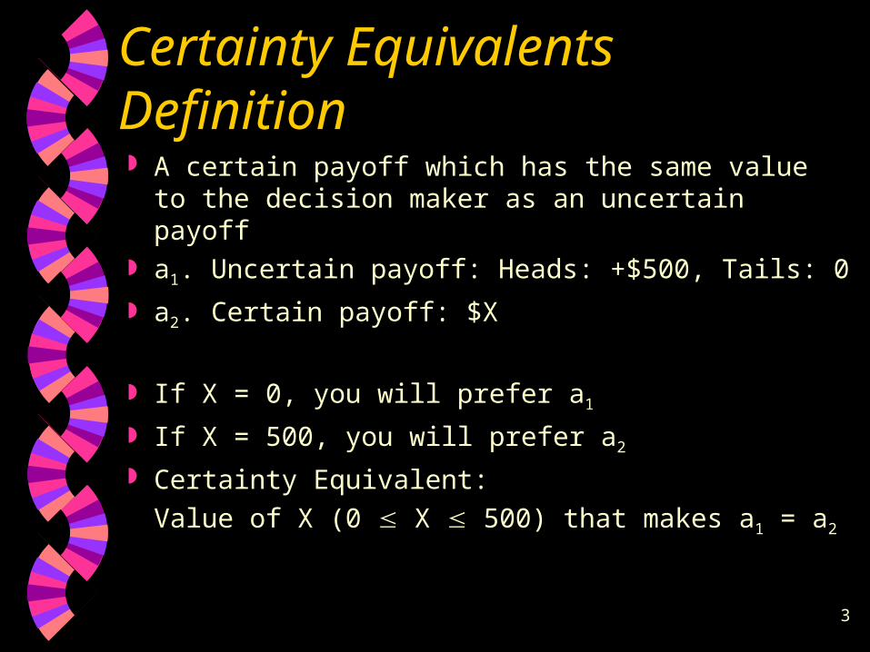
Certainty Equivalents Definition

A certain payoff which has the same value to the decision maker as an uncertain payoff

a1. Uncertain payoff: Heads: +$500, Tails: 0

a2. Certain payoff: $X

If X = 0, you will prefer a1

If X = 500, you will prefer a2

Certainty Equivalent:

Value of X (0 X 500) that makes a1 = a2

4

Determining & Using CE

In general, given 2 choices: a1. $X with probability p, or $Y with prob. (1 – p)

a2. $Z for certain (X Z Y)

The value of Z that makes the 2 options equal to decision maker is the:

Certainty equivalent of a1 : CE(a1)

Stochastic problems can be transformed to deterministic equivalent

Criterion: select option aj with maximum CE(aj)

5

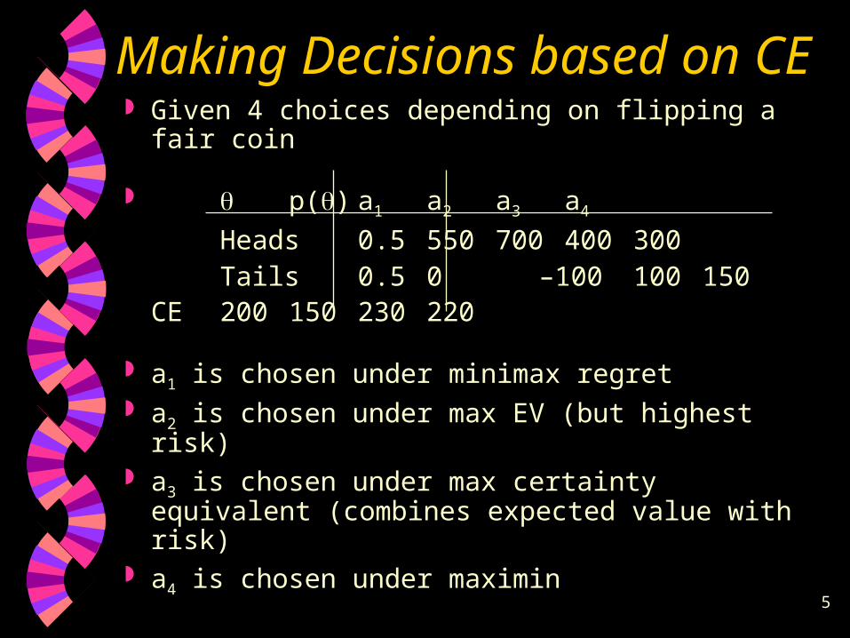
Making Decisions based on CE Given 4 choices depending on flipping a fair coin

p() a1 a2 a3 a4

Heads 0.5 550 700 400 300 Tails 0.5 0 –100 100 150

CE 200 150 230 220

a1 is chosen under minimax regret a2 is chosen under max EV (but highest risk) a3 is chosen under max certainty equivalent

(combines expected value with risk) a4 is chosen under maximin

6

Certainty Equivalents & Coherence

The concept of CE provides a coherent approach for evaluating (ranking) decisions

A valid criterion must recommend ranking consistent with the CE options

A coherent criterion must provide the same score for an uncertain option and its certainty equivalent

7

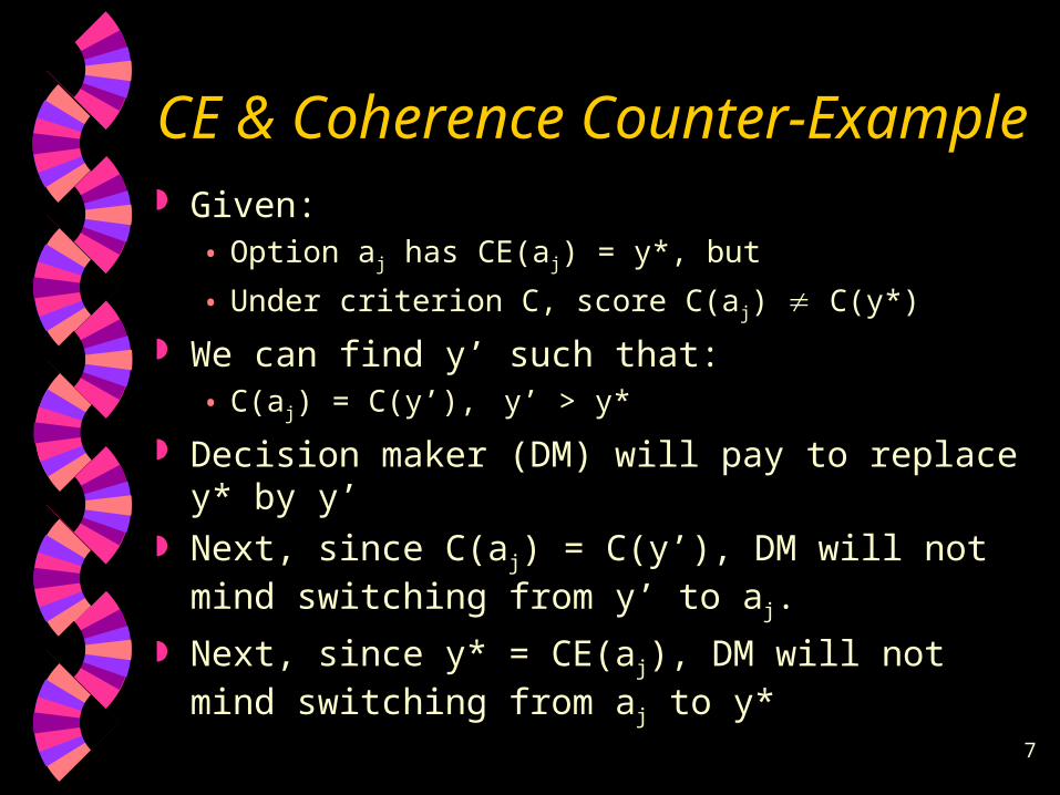
CE & Coherence Counter-Example Given:

• Option aj has CE(aj) = y*, but

• Under criterion C, score C(aj) C(y*)

We can find y’ such that:• C(aj) = C(y’), y’ > y*

Decision maker (DM) will pay to replace y* by y’ Next, since C(aj) = C(y’), DM will not mind

switching from y’ to aj.

Next, since y* = CE(aj), DM will not mind switching from aj to y*

8

CE & Coherence Counter-Example

Example shows that an incoherent criterion makes DM a perpetual money-making machine

For coherence: y’ = y*

Any evaluation criterion must be subjected to this coherence test

Can we use only CE criterion for all decision problems?

No, only for simple 2-outcome problems

9

CE for complex problems

Given: p() a1

Excellent 0.1 10,000Good 0.3 5,000Average 0.3 1,000Poor 0.2 – 400Terrible 0.1 – 3,000

Evaluating CE(a1) is extremely difficult Utility theory is used for complex problems

10

3.2. Utility Functions Utility:

Relative value (worth) of each payoff to the decision maker

Utility Theory:

Transform payoffs into utility scale (0 1)

Utility & Coherence:

Expected utility criterion EU(aj) ranking of options is consistent with DM certainty equivalents EU(aj)

11

Evaluating utility functions

Given:

p() a1 a2

Good 0.3 $1000 $800 Average 0.4 $500 $600

Poor 0.3 $300 $400

Min payoff = $300, Max payoff = $1000 Range of payoffs (300 1000)

U(300) = 0U(1000) = 1

12

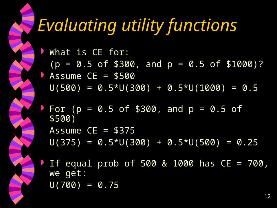
Evaluating utility functions

What is CE for:(p = 0.5 of $300, and p = 0.5 of $1000)?

Assume CE = $500U(500) = 0.5*U(300) + 0.5*U(1000) = 0.5

For (p = 0.5 of $300, and p = 0.5 of $500)Assume CE = $375U(375) = 0.5*U(300) + 0.5*U(500) = 0.25

If equal prob of 500 & 1000 has CE = 700, we get:U(700) = 0.75

13

Evaluating utility functions

y 300 375 500 700 1000 U(y) 0 0.25 0.5 0.75 1.0 1

300 375 500 700 1000 y

14

Converting payoffs to utilities

Utility matrix, using interpolation:

p() a1 a2

Good 0.3 1 0.85 Average 0.4 0.5 0.65

Poor 0.3 0 0.33EU 0.5 0.61

Since U(375) = 0.25 & U(500) = 0.5U(400) = 0.25 + [(400-375)/(500-375)]*(0.5-0.25) = 0.3

Based on EU, choose a2

15

Steps in using utility functions

1. Derive the utility function using simple CE questions

2. Transform payoffs into utilities

3. Choose decision with max expected utility

16

Utility Ex 1: Oil exploration

Decisions:Alternative investment strategies in oil exploration

To evaluate utility, 2 options:

a1. Invest $X to explore for oil prob p: you get $Y, prob (1 – p): you get 0

a2. Do not invest

What probability p would make you indifferent?

17

Utility Ex 2: Education planning

Decisions:Alternative reading improvement programs

Payoff:Average reading performance

Utility function changes slope around national average (50%)Risk = doing worse than national averageShape of utility function indicates risk attitude

18

3.3. Risk Attitudes

Given 2 choices: p() a1 a2

Heads 0.5 500 200 Tails 0.5 0 200

If 2 options are equivalent to you, i.e.,

CE(a1) = 200, then

CE(a1) = 200 < EV(a1) = 250

You considered are risk averse (avoider)

19

Risk Premium Risk Premium

Money DM is willing to pay to avoid uncertainty (risk)

RP(y) = EV(y) – CE(y)= 250 – 200 = 50

3 risk attitudes:• Risk-Averse: RP(y) > 0• Risk-Neutral: RP(y) = 0• Risk-Seeking: RP(y) < 0

20

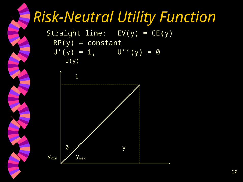
Risk-Neutral Utility FunctionStraight line: EV(y) = CE(y)

RP(y) = constantU’(y) = 1, U’’(y) = 0

U(y) 1

0 y

ymin ymax

21

Risk-Averse Utility FunctionConcave line: EV(y) > CE(y)

RP(y) > 0U’(y) > 0, U’’(y) 0

U(y) 1

y

ymin ymax

22

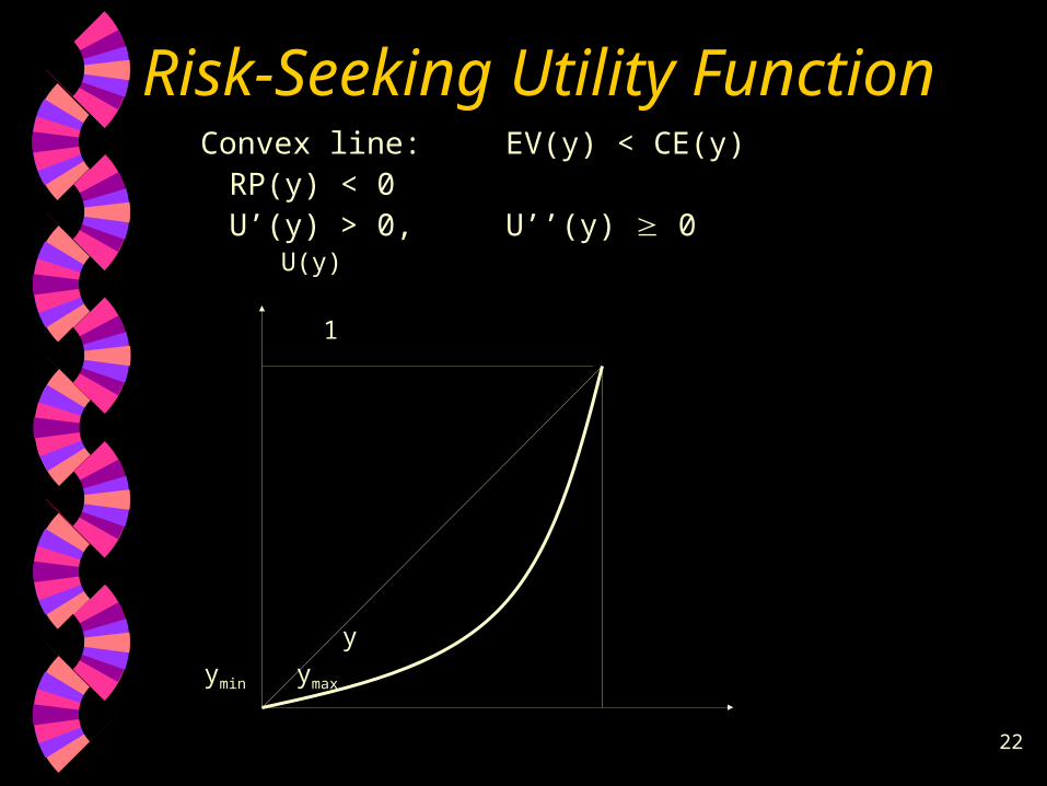
Risk-Seeking Utility FunctionConvex line: EV(y) < CE(y)

RP(y) < 0U’(y) > 0, U’’(y) 0

U(y) 1

y

ymin ymax

23

Risk Attitude Example

Given 2 options: a1. Uncertain payoff: Heads: +$500, Tails: 0

a2. Certain payoff: $X

What value of X would make 2 options equivalent? Risk averse: X = 200 RP = 50 Risk neutral:X = 250 RP = 0 Risk seeking: X = 300 RP = – 50

24

Applications of Risk Attitude

Risk AversionMost common approach in significant decisions

Risk neutrality Corresponds to expected value criterion. Should be used in routine, non-significant decisions

Risk attitude may:- change over time- increase with increasing capital

25

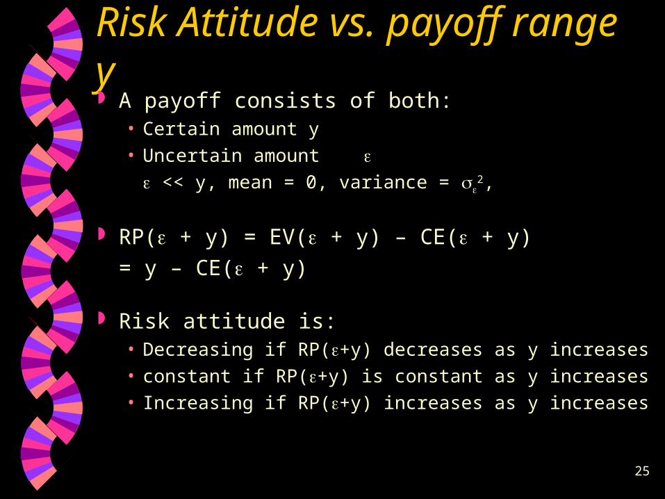
Risk Attitude vs. payoff range y A payoff consists of both:

• Certain amount y

• Uncertain amount

<< y, mean = 0, variance = 2,

RP( + y) = EV( + y) – CE( + y)

= y – CE( + y)

Risk attitude is:• Decreasing if RP(+y) decreases as y increases

• constant if RP(+y) is constant as y increases

• Increasing if RP(+y) increases as y increases

26

Risk Attitude vs. payoff range y

Constant risk attitude (premium)

Constantly risk-averseU(y) = a – be– ry, r > 0, a & b constants

Constantly risk-neutralU(y) = a + by, a & b constants

Constantly risk-averseU(y) = a + be– ry, r < 0, a & b constants

27

Risk Attitude vs. payoff range y Decreasing risk attitude

Risk aversion (premium) decreases with increasing capital

U(y) = – e– ay – be– cy, a > 0, bc > 0

Decreasing risk attitude

Risk aversion (premium) proportional to yRP( + y) = a + by

28

Risk Aversion Function r(y) = – U’’(y)/U’(y) RP( + y) 0.5

2 r(y) ExampleGiven:

U(y) = a + by – cy2, b, c > 0, 0 < y < b/2c

U’(y) = b – 2cyU’’(y) = – 2cr(y) = 2c/(b – 2cy)

RP( + y) = c2/(b – 2cy) > 0

(increasing risk attitude)

29

3.4. Theoretical Assumptions of Utility

Preceding sections: • How utility works

This section: • Why utility works• Theoretical basis• Basic assumptions

30

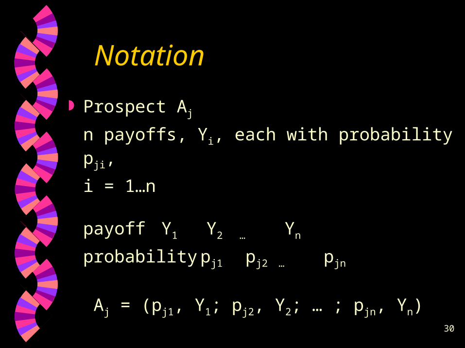
Notation

Prospect Aj

n payoffs, Yi, each with probability pji,

i = 1…n

payoff Y1 Y2 … Yn

probabilitypj1 pj2 … pjn

Aj = (pj1, Y1; pj2, Y2; … ; pjn, Yn)

31

Notation

Compound Prospect Ck

m prospects, Aj, each with probability qkj, j = 1…m

prospect A1 A2 … Am

probabilityqk1 qk2 … qkm

Ck = (qk1, A1; qk2, A2; … ; qkm, Am)

32

Notation example

A1: fair coin

Heads (p11 = 0.5) Y1 = 20

Tails: (p12 = 0.5) Y2 = – 10

A2: bent coin

Heads (p21 = 0.3) Y1 = 20

Tails: (p22 = 0.7) Y2 = – 10

C1: fair die

even: 2, 4, 6 (q11 = 0.5) A1

Odd: 1, 3, 5 (q12 = 0.5) A2

33

Assumption 1 (Structure)

It is sufficient to describe the choices open to the decision maker in terms of payoff values and their associated probabilities

Reducing the problem to prospects and compound prospects captures all that is essential to the decision maker

Temporal resolution of uncertainty:The decision maker may choose between 2 alternatives with exactly the same payoffs and probabilities based on different payoff times

34

Assumption 2 (Ordering) The decision maker may express preference or

indifference between any pair of payoffs

Notation Y1 > Y2 Y1 is preferred to Y2

Y1 Y2 Y1 is preferred to or same as Y2

Y2 is not preferred to Y1•

Y* = best payoff, Y* = worst payoff

Transitivity:If A1 A2 and A2 A3 then A1 A3

35

Assumption 3 (Reduction of Compound Prospects)

Any compound prospect should be indifferent to its equivalent simple prospect

Ck (qk1, A1; qk2, A2; … ; qkm, Am)

[qk1(p11, Y1; p12, Y2; … ; p1n, Yn);

qk2(p21, Y1; p22, Y2; … ; p2n, Yn); . . .

qkm(pm1, Y1; pm2, Y2; … ; pmn, Yn)]

(p'k1, Y1; p'k2, Y2; … ; p'km, Ym) Where

p'kj = qk1p1j + qk2p2j + . . . + qkmpmj

36

Assumption 3 example C1: fair die

q1j Aj p1j Y1 p2j Y2

q11 = 0.5 A1: fair coin 0.5 20 0.5 –10

q12 = 0.5 A2: bent coin 0.3 20 0.7 –10

C1 (0.5, A1; 0.5, A2) [0.5(0.5, 20; 0.5, –10); 0.5(0.3, 20; 0.7, –10)]

[(0.25 + 0.15), 20; (0.25 + 0.35), –10] [0.4, 20; 0.6, –10]

37

Assumption 3 & Coherence

Assumption 3 indicates ideal level of coherence

No preference for single or multiple steps

Assumption 3 does not apply if• Preference for multiple steps, game atmosphere• Special type of risk in a particular business

38

Assumption 4 (Continuity) Every payoff Yi can be considered a certainty

equivalent for a prospect:

[ui, Y*; (1 – ui), Y*], 0 ui 1

Y* = best payoff, Y* = worst payoff

Since each uncertain prospect has an equivalent certain payoff (CE),

then each certain payoff has an equivalent uncertain prospect

39

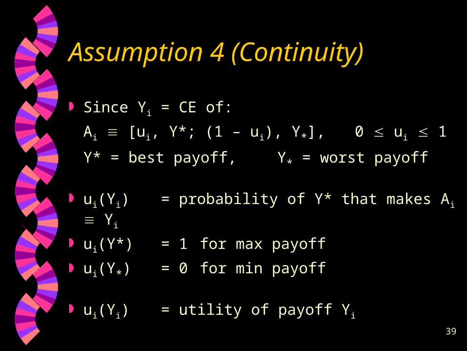
Assumption 4 (Continuity)

Since Yi = CE of:

Ai [ui, Y*; (1 – ui), Y*], 0 ui 1

Y* = best payoff, Y* = worst payoff

ui(Yi) = probability of Y* that makes Ai Yi

ui(Y*)= 1 for max payoff

ui(Y*) = 0 for min payoff

ui(Yi) = utility of payoff Yi

40

Assumption 5 (Substitutability)

In any prospect, Yi can be substituted by its a uncertain equivalent:

[ui, Y*; (1 – ui), Y*]

Yi and [ui, Y*; (1 – ui), Y*] are indifferent,

not only when considered alone, but also when considered part of a more complicated prospect

Similar to coherence related to minimax regret: ranking of alternatives should not change if other alternatives are added

41

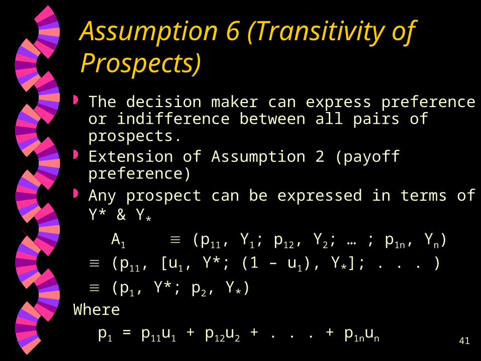
Assumption 6 (Transitivity of Prospects)

The decision maker can express preference or indifference between all pairs of prospects.

Extension of Assumption 2 (payoff preference) Any prospect can be expressed in terms of Y* &

Y*

A1 (p11, Y1; p12, Y2; … ; p1n, Yn)

(p11, [u1, Y*; (1 – u1), Y*]; . . . )

(p1, Y*; p2, Y*)

Where

p1 = p11u1 + p12u2 + . . . + p1nun

42

Assumption 7 ( Monotonicity)

A prospect Ar [pr, Y*; (1 – pr), Y*]

is preferred or indifferent to ( )

prospect As [ps, Y*; (1 – ps), Y*] iff: pr ps

Given 2 options with the same 2 alternative payoffs, we prefer the option with higher probability of the better payoff

For options with several payoffs: Ar As iff:pr1 u1 + pr2 u2 + . . . + pr1 un ps1 u1 + ps2 u2 + . . . + ps1 un

EU(Ar) EU(As)

43

3.5. Some Caveats in Interpreting Utility

Utility theory is normative:• It suggests what people should do to be

coherent• Does not describe what they actually do

In practice, people violate expected utility criterion depending on circumstances

44

Utilities do not add up

Expected utility of a sum of payoff is not equal to sum of expected utilities

U(A + B) U(A) + U(B)

Unless the decision maker is risk-neutral

45

Utility differences do not express strength of preferences

Given: Y1 > Y2 > Y3 > Y4 , and

U(Y1 – Y2 ) > U(Y3 – Y4)

This does not imply moving from Y2 to Y1 is preferable to moving from Y4 to Y3.

Utility provides an “ordinal” scale, not an “interval” scale• Ordinal: teacher evaluation, (7 – 6) (9 – 8)• Interval: weight in kilograms, (60 – 50) = (80 – 70)

46

Utilities are not comparable from person to person If 2 people assign the same utility to a

prospect,

we cannot say it has the same worth to each

Utility values are completely subjective

Utilities of different people cannot be added to determine group preferences

47

3.6. Issues in the assessment of risk

Utility assessment is not a natural activity for DM

Unnatural setup may results in wrong utility values, and wrong decisions

Method of assessment must be as close as possible to real problem

48

Basic utility assessment process

Given 2 options:• X certain payoff• Y probability p of payoff G (gain)

probability (1 – p) of payoff L (loss)

Four variables• X, Y, G, L• Fix any 3 variables, ask DM to supply the 4th

49

4 Response modes

Certainty equivalence: DM gives X Probability equivalence: DM gives p Gain equivalence: DM gives G Loss equivalence: DM gives L

First 2 methods most common

50

Level of probabilty

4 variables: X, p, G, L

Except in probability equivalence methods, p is given

Small probabilities get distorted

p = 1 – p = 0.5 seems to be least biased

51

Levels of payoff

Initial G and L are Ymax and Ymin, but values inside interval are arbitrary

Moving from outside to inside creates bias to risk aversion

Adjustment biasA new assessment is made by adjusting the previous one, this adjustment is not enough

Solution: get assessments at different times

52

Assumptions or transfer of risk

If both G and L are losses, the question is:• Facing either a loss of G (prob. p) or a loss of L

(prob. 1 – p), how much would you pay to have it removed?

• Transfer uncertain (risky) loss to a certain loss

Inertia bias: • Tendency to stay with current situation unless

alternative is clearly better

53

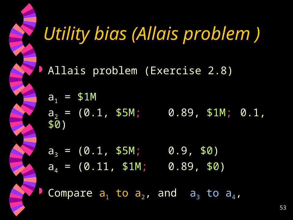
Utility bias (Allais problem )

Allais problem (Exercise 2.8)

a1 = $1M

a2 = (0.1, $5M; 0.89, $1M; 0.1, $0)

a3 = (0.1, $5M; 0.9, $0)

a4 = (0.11, $1M; 0.89, $0)

Compare a1 to a2, and a3 to a4,

54

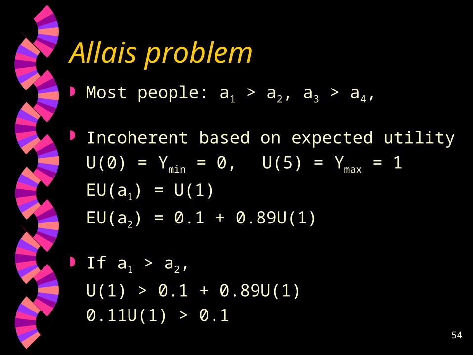
Allais problem Most people: a1 > a2, a3 > a4,

Incoherent based on expected utility

U(0) = Ymin = 0, U(5) = Ymax = 1

EU(a1) = U(1)

EU(a2) = 0.1 + 0.89U(1)

If a1 > a2,

U(1) > 0.1 + 0.89U(1)

0.11U(1) > 0.1

55

Allais problem

EU(a3) = 0.1

EU(a4) = 0.11U(1)

If a3 > a4,

0.1 > 0.11U(1)

This contradicts the result for a1 > a2,

56

Certainty effect

Reason for inconsistency in Allais example People overestimate a certain payoff

compared to expected utility Expected utility should not be taken for

granted• Consistency checks• Sensitivity analysis• Estimate utility to same no. of significant

figures as payoff values Y