1 chapter 3 solving problems by searching. 2 outline problem-solving agentsproblem-solving agents...
TRANSCRIPT
1
Chapter 3
Solving Problems by Solving Problems by SearchingSearching
2
OutlineOutline
• Problem-solving agentsProblem-solving agents
• Problem typesProblem types
• Problem formulationProblem formulation
• Example problemsExample problems
• Basic search algorithmsBasic search algorithms

3
8-puzzle problem8-puzzle problem
– state descriptionstate description• 3-by-3 array: each cell contains one of 1-8 or blank symbol
– two state transition descriptionstwo state transition descriptions• 84 moves: one of 1-8 numbers moves up, down, right, or left
• 4 moves: one black symbol moves up, down, right, or left
– The number of nodes in the state-space graph:The number of nodes in the state-space graph:• 9! ( = 362,880 )
57
461
382
567
48
321
4
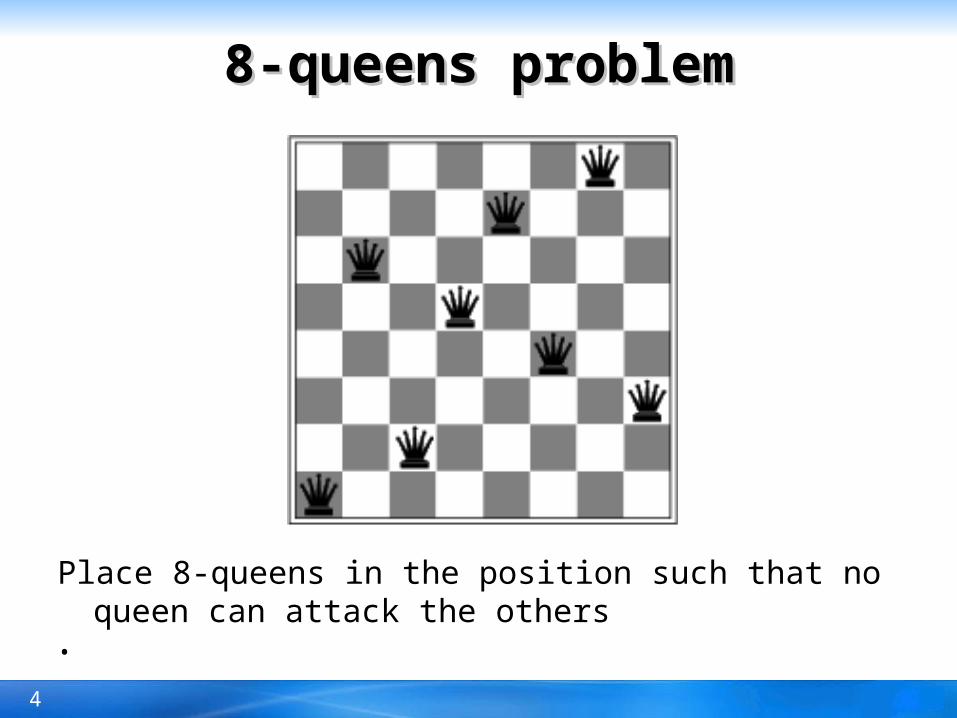
8-queens problem8-queens problem
Place 8-queens in the position such that no queen can attack the others
•
5
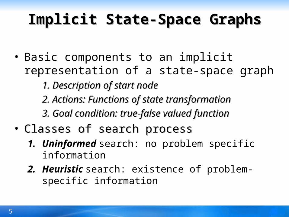
Implicit State-Space GraphsImplicit State-Space Graphs
• Basic components to an implicit representation of a state-space graph
1. Description of start node1. Description of start node
2. Actions: Functions of state transformation2. Actions: Functions of state transformation
3. Goal condition: true-false valued function3. Goal condition: true-false valued function
• Classes of search processClasses of search process1. Uninformed search: no problem specific information
2. Heuristic search: existence of problem-specific information
6
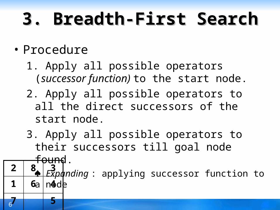
3. Breadth-First Search3. Breadth-First Search
• Procedure1. Apply all possible operators (successor function) to
the start node.
2. Apply all possible operators to all the direct successors of the start node.
3. Apply all possible operators to their successors till goal node found. Expanding : applying successor function to a node
57
461
382

7
57
461
382

8
Breadth-First SearchBreadth-First Search
• AdvantageAdvantage– Finds the path of minimal length to the goal.
• DisadvantageDisadvantage– Requires the generation and storage of a tree whose
size is exponential the the depth of the shallowest goal node
• Uniform-costUniform-cost search [Dijkstra 1959]– Expansion by equal cost rather than equal depth

9
Problem-solving agentsProblem-solving agents

10
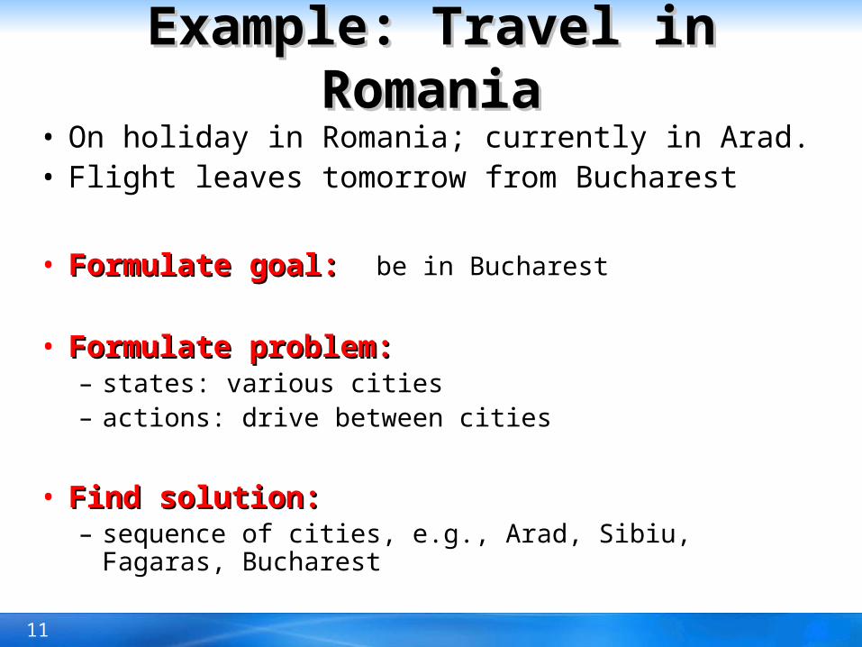
Example: Travel in RomaniaExample: Travel in Romania
11
Example: Travel in RomaniaExample: Travel in Romania• On holiday in Romania; currently in Arad.• Flight leaves tomorrow from Bucharest
• Formulate goal: Formulate goal: be in Bucharest
• Formulate problem: Formulate problem: – states: various cities– actions: drive between cities
• Find solution:Find solution:– sequence of cities, e.g., Arad, Sibiu, Fagaras, Bucharest

12
Problem typesProblem types• Deterministic, fully observable single-state problem
– Agent knows exactly which state it will be in; solution is a sequence
• Non-observable sensorless problem (conformant problem)– Agent may have no idea where it is; solution is a sequence
• Nondeterministic and/or partially observable contingency problem– percepts provide new information about current state– often interleave, search, execution
• Unknown state space exploration problem

13
Single-state problem formulationSingle-state problem formulationA A problemproblem is defined by four items: is defined by four items:
1.1. initial state e.ginitial state e.g., "at Arad“
2.2. actions or actions or successor function S(x) = set of action–state pairs – e.g., S(Arad) = {<Arad Zerind, Zerind>, … }
3.3. goal testgoal test, can be– explicitexplicit, e.g., x = "at Bucharest"– implicitimplicit, e.g., Checkmate(x)
4.4. path cost path cost (additive)– e.g., sum of distances, number of actions executed, etc.– c(x,a,y) is the step cost, assumed to be ≥ 0
• A A solutionsolution is a sequence of actions leading from the initial state is a sequence of actions leading from the initial state to a goal stateto a goal state

14
Selecting a state spaceSelecting a state space• Real world is very complex generally
state space must be abstracted for problem solving
• (Abstract) state = set of real states
• (Abstract) action = complex combination of real actions– e.g., "Arad Zerind" represents a complex set of possible routes,
detours, rest stops, etc.
• For guaranteed realizability, any real state "in Arad“ must get to some real state "in Zerind“
• (Abstract) solution (Abstract) solution = – set of real paths that are solutions in the real world
• Each abstract action should be "easier" than the original problem
–

15
Example: robotic assemblyExample: robotic assembly
• states?: real-valued coordinates of robot joint angles parts of the object to be assembled
• goal test?: complete assembly
• path cost?: time to execute• actions?: continuous motions of robot joints

16
Tree search algorithmsTree search algorithms
• Basic idea:– offline, simulated exploration of state space by generating
successors of already-explored states (a.k.a.~expanding states)
–

17
Tree search exampleTree search example

18
Tree search exampleTree search example

19
Tree search exampleTree search example
20
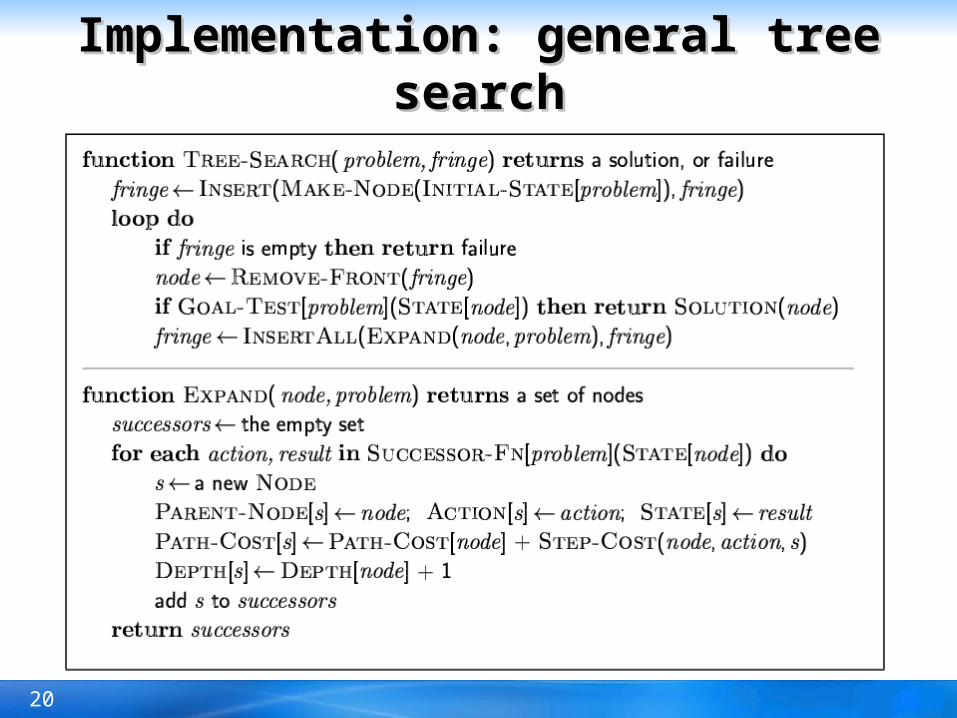
Implementation: general tree searchImplementation: general tree search

21
Implementation: states vs. nodesImplementation: states vs. nodes
• A state is a (representation of) a physical configuration• A node is a data structure constituting part of a search tree
includes state, parent node, action, path cost g(x), depth
• The Expand function creates new nodes, filling in the various fields and using the SuccessorFn of the problem to create the corresponding states.
22
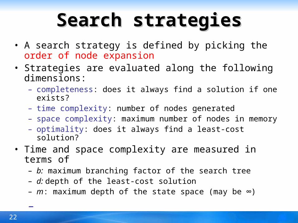
Search strategiesSearch strategies• A search strategy is defined by picking the order of node
expansion• Strategies are evaluated along the following dimensions:
– completeness: does it always find a solution if one exists?– time complexity: number of nodes generated– space complexity: maximum number of nodes in memory– optimality: does it always find a least-cost solution?
• Time and space complexity are measured in terms of – b: maximum branching factor of the search tree– d: depth of the least-cost solution– m: maximum depth of the state space (may be ∞)
–

23
Uninformed search strategiesUninformed search strategies• Uninformed search strategies use only the information available
in the problem definition
• Breadth-first search
• Uniform-cost search
• Depth-first search
• Depth-limited search
• Iterative deepening search

24
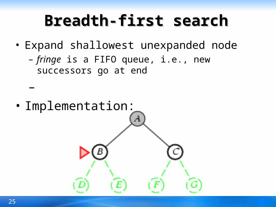
Breadth-first searchBreadth-first search
• Expand shallowest unexpanded node– fringe is a FIFO queue, i.e., new successors go at end
–
• Implementation:
25
Breadth-first searchBreadth-first search
• Expand shallowest unexpanded node– fringe is a FIFO queue, i.e., new successors go at end
–
• Implementation:

26
Breadth-first searchBreadth-first search• Expand shallowest unexpanded node
– fringe is a FIFO queue, i.e., new successors go at end
–
• Implementation:
27
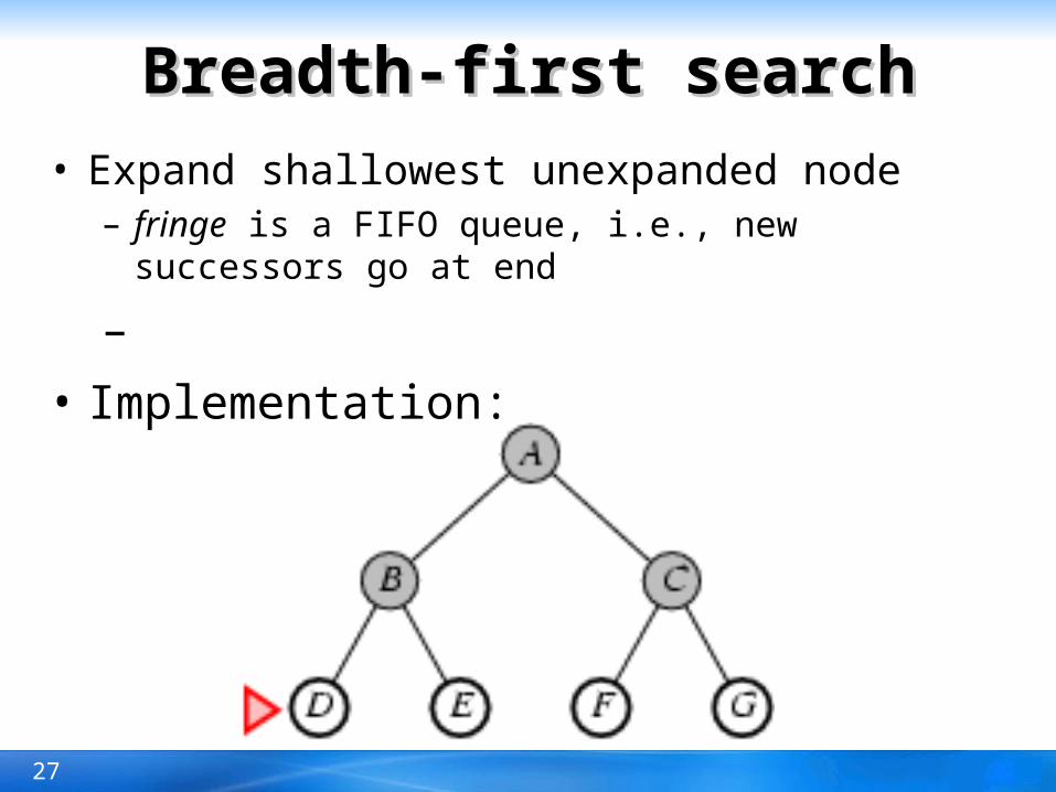
Breadth-first searchBreadth-first search• Expand shallowest unexpanded node
– fringe is a FIFO queue, i.e., new successors go at end
–
• Implementation:

28
Properties of breadth-first searchProperties of breadth-first search
• Complete? Yes (if b is finite)
• Time? 1+b+b2+b3+… +bd + b(bd-1) = O(bd+1)
• Space? O(bd+1) (keeps every node in memory)
• Optimal? Yes (if cost = 1 per step)
• Space is the bigger problem (more than time)
•

29
Uniform-cost searchUniform-cost search• Expand least-cost unexpanded node
– fringe = queue ordered by path cost
• Equivalent to breadth-first if step costs all equal
• Space? # of nodes with g ≤ cost of optimal solution, O(bceiling(C*/ ε))
• Optimal? Yes – nodes expanded in increasing order of g(n)
• Complete? Yes, if step cost ≥ ε
• Time? # of nodes with g ≤ cost of optimal solution, O(bceiling(C*/ ε)) where C* is the cost of the optimal solution
• Implementation:

30
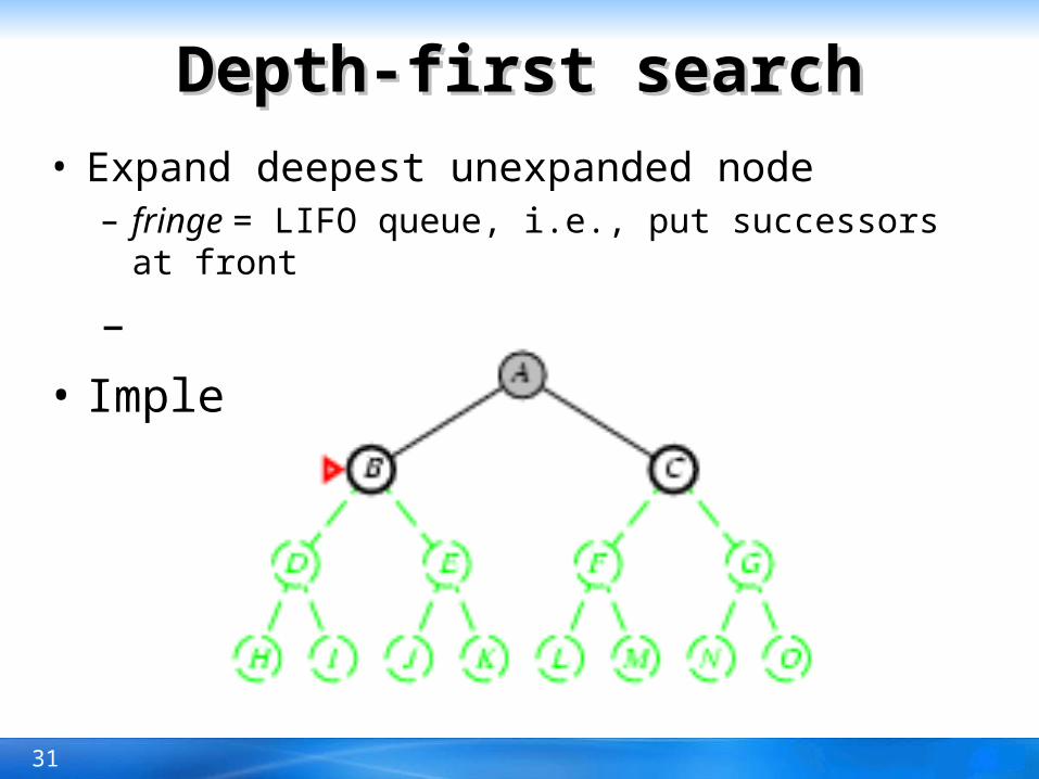
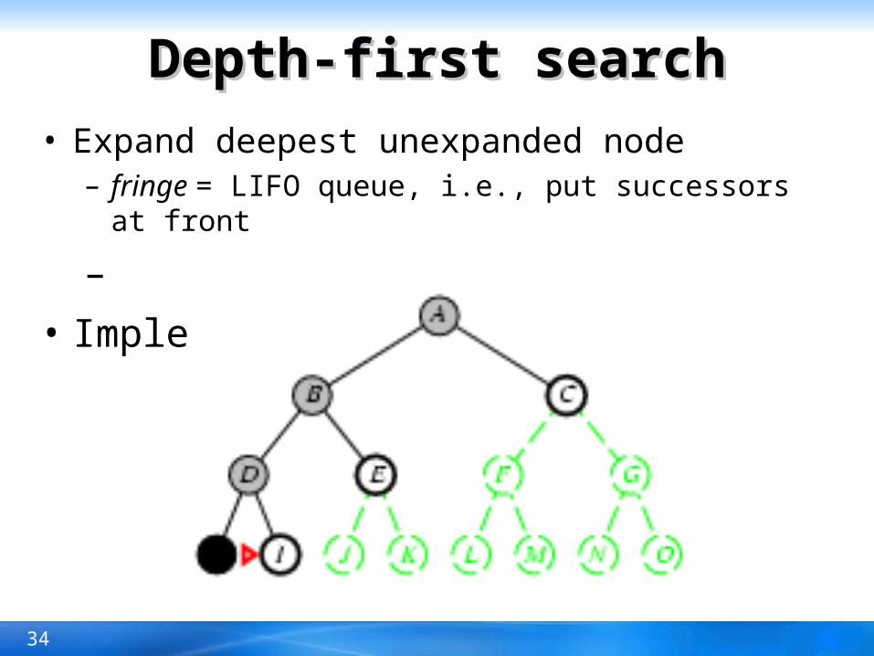
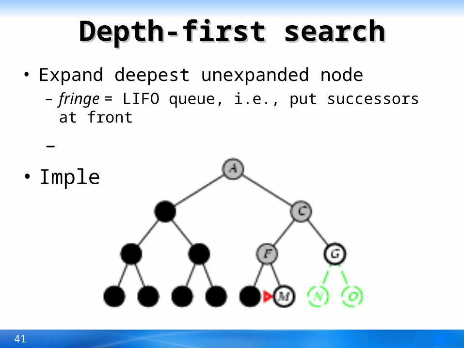
Depth-first searchDepth-first search• Expand deepest unexpanded node
– fringe = LIFO queue, i.e., put successors at front
–
• Implementation:
31
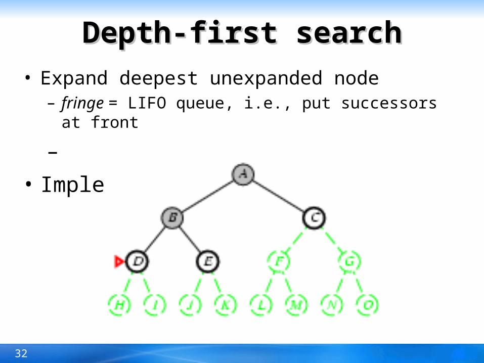
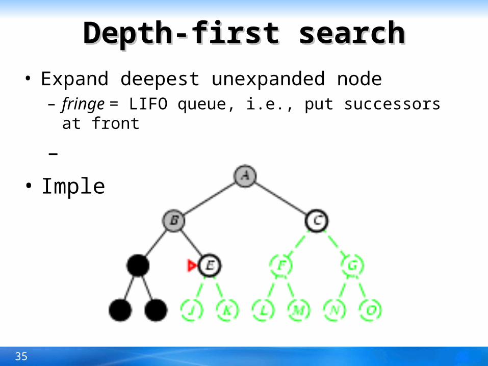
Depth-first searchDepth-first search• Expand deepest unexpanded node
– fringe = LIFO queue, i.e., put successors at front
–
• Implementation:
32
Depth-first searchDepth-first search• Expand deepest unexpanded node
– fringe = LIFO queue, i.e., put successors at front
–
• Implementation:

33
Depth-first searchDepth-first search• Expand deepest unexpanded node
– fringe = LIFO queue, i.e., put successors at front
–
• Implementation:
34
Depth-first searchDepth-first search• Expand deepest unexpanded node
– fringe = LIFO queue, i.e., put successors at front
–
• Implementation:
35
Depth-first searchDepth-first search• Expand deepest unexpanded node
– fringe = LIFO queue, i.e., put successors at front
–
• Implementation:

36
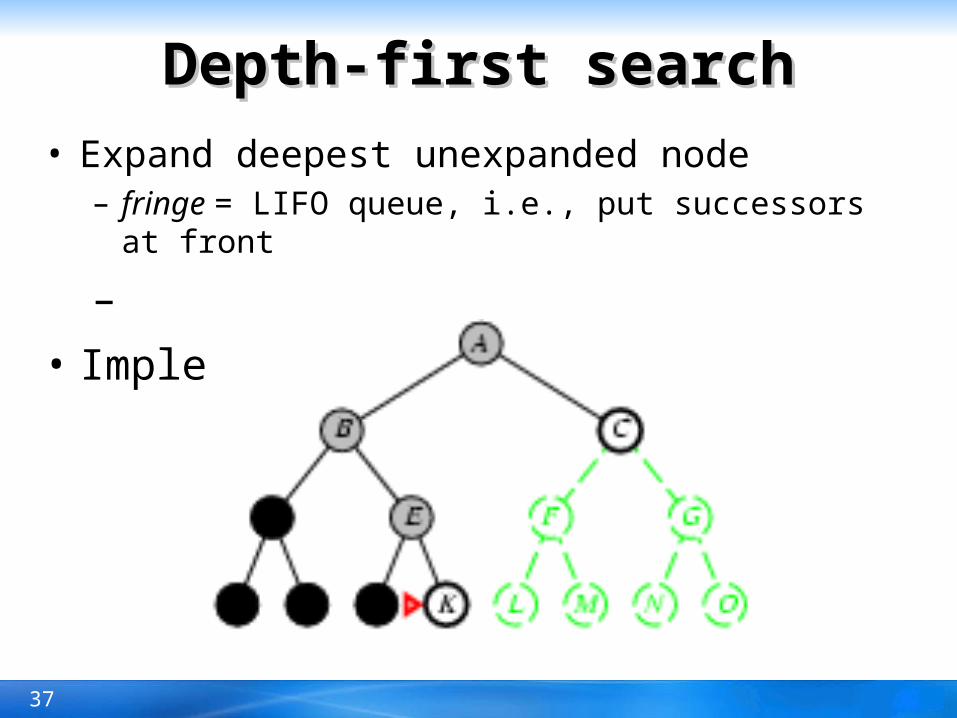
Depth-first searchDepth-first search• Expand deepest unexpanded node
– fringe = LIFO queue, i.e., put successors at front
–
• Implementation:
37
Depth-first searchDepth-first search• Expand deepest unexpanded node
– fringe = LIFO queue, i.e., put successors at front
–
• Implementation:

38
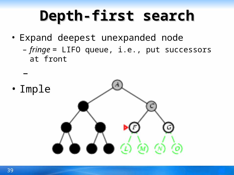
Depth-first searchDepth-first search• Expand deepest unexpanded node
– fringe = LIFO queue, i.e., put successors at front
–
• Implementation:
39
Depth-first searchDepth-first search• Expand deepest unexpanded node
– fringe = LIFO queue, i.e., put successors at front
–
• Implementation:

40
Depth-first searchDepth-first search• Expand deepest unexpanded node
– fringe = LIFO queue, i.e., put successors at front
–
• Implementation:
41
Depth-first searchDepth-first search• Expand deepest unexpanded node
– fringe = LIFO queue, i.e., put successors at front
–
• Implementation:
42
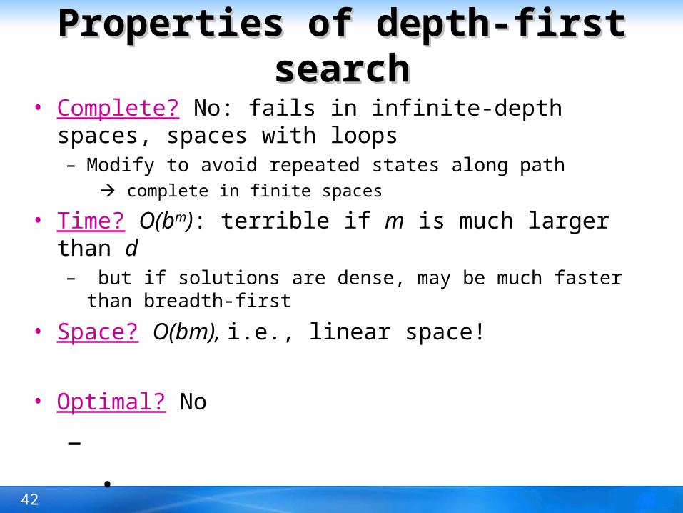
Properties of depth-first searchProperties of depth-first search
• Complete? No: fails in infinite-depth spaces, spaces with loops– Modify to avoid repeated states along path
complete in finite spaces
• Time? O(bm): terrible if m is much larger than d– but if solutions are dense, may be much faster than breadth-first
• Space? O(bm), i.e., linear space!
• Optimal? No
–•
–

43
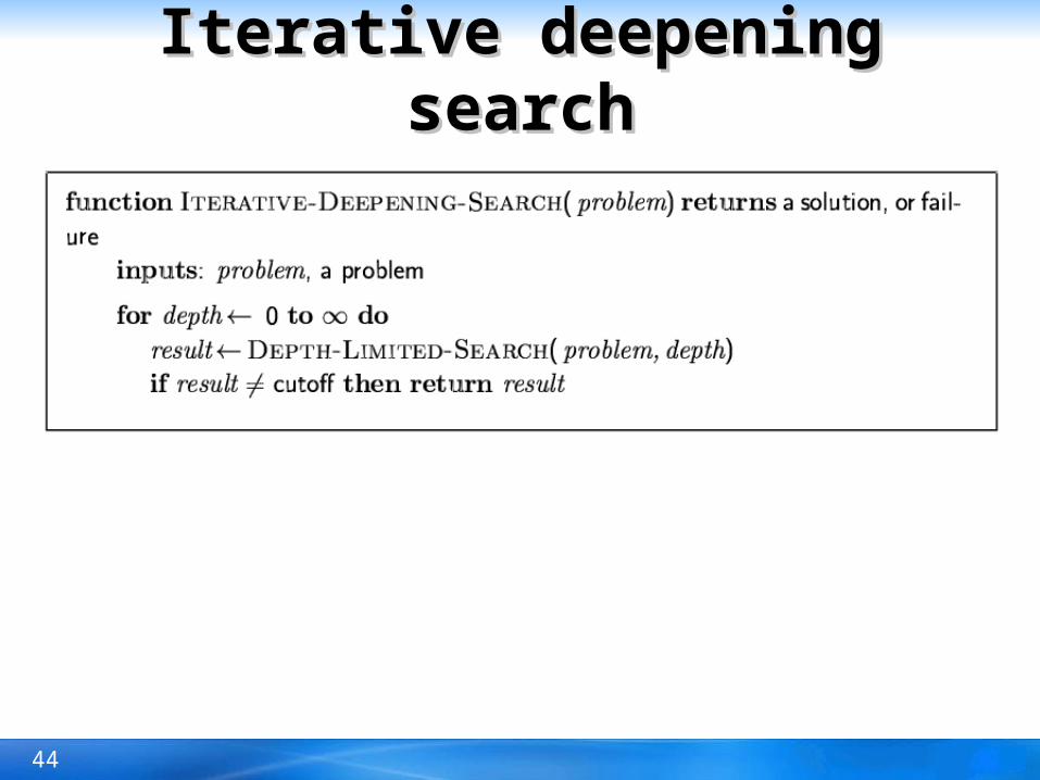
Depth-limited searchDepth-limited search= depth-first search with depth limit l,
• i.e., nodes at depth l have no successors
Recursive implementation:
44
Iterative deepening searchIterative deepening search
4545
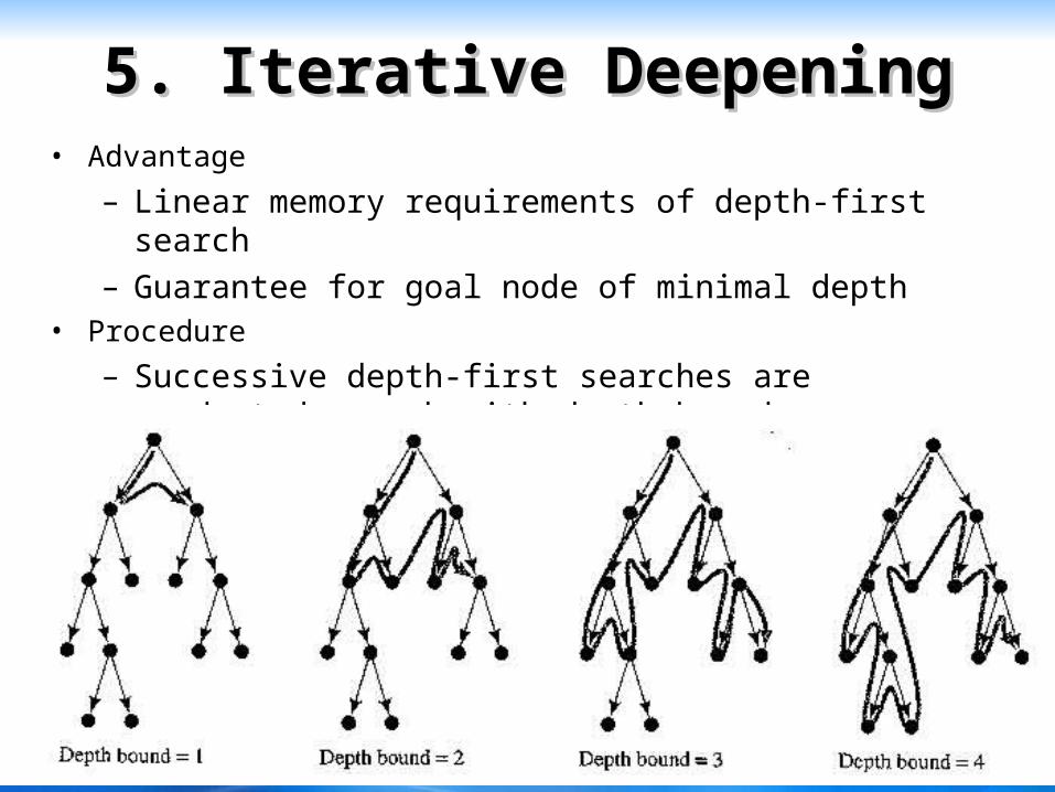
5. Iterative Deepening5. Iterative Deepening• Advantage
– Linear memory requirements of depth-first search
– Guarantee for goal node of minimal depth• Procedure
– Successive depth-first searches are conducted – each with depth bounds increasing by 1

46
Iterative deepening searchIterative deepening search• Number of nodes generated in a depth-limited search to depth d
with branching factor b:
NDLS = b0 + b1 + b2 + … + bd-2 + bd-1 + bd
• Number of nodes generated in an iterative deepening search to depth d with branching factor b:
NIDS = (d+1)b0 + d b^1 + (d-1)b^2 + … + 3bd-2 +2bd-1 + 1bd
• For b = 10, d = 5,– NDLS = 1 + 10 + 100 + 1,000 + 10,000 + 100,000 = 111,111
– NIDS = 6 + 50 + 400 + 3,000 + 20,000 + 100,000 = 123,456
• Overhead = (123,456 - 111,111)/111,111 = 11%

47
Iterative Iterative deepeningdeepening search search• Complete? Yes
• Time? (d+1)b0 + d b1 + (d-1)b2 + … + bd = O(bd)
• Space? O(bd)
• Optimal? Yes, if step cost = 1

48
Summary of algorithmsSummary of algorithms

49
Problem: Repeated statesProblem: Repeated states
• Failure to detect repeated states can turn a linear problem into an exponential one!

50
Graph searchGraph search
51
SummarySummary• Problem formulation usually requires abstracting away Problem formulation usually requires abstracting away
real-world details to define a state space that can real-world details to define a state space that can feasibly be exploredfeasibly be explored
• Variety of uninformed search strategiesVariety of uninformed search strategies
• Iterative deepening search uses only linear space and Iterative deepening search uses only linear space and not much more time than other uninformed algorithmsnot much more time than other uninformed algorithms