1 codes, ciphers, and cryptography-ch 2.3 michael a. karls ball state university

1

Codes, Ciphers, and Cryptography-Ch 2.3

Michael A. Karls

Ball State University

2

The Friedman Test

The Kasiski Test is a method to determine the length of a Vigenère cipher keyword via distances between repeated sequences of ciphertext.

The Friedman Test, which was developed by Colonel William Friedman in 1925, uses probability to determine whether a ciphertext has been enciphered using a monoalphabetic or polyalphabetic substitution cipher.

Another use of the Friedman Test is to find the length of a Vigenère cipher keyword!

3

Basic Probability Concepts

Formally, the study of probability began with the posthumous publication of Girolamo Cardano’s “Book on Games and Chance” in 1663.

Probably he wrote it in ~1563. Recall Cardano also worked with grids for encryption! Other “key” players in the development of this

branch of mathematics include: Blaise Pascal and Pierre de Fermat (17th century). Jakob Bernoulli (late 17th century).

4

Definition of Probability

One way to define probability is as follows: The probability of an event E is a quantified

assessment of the likelihood of E. By quantified, we mean a number is assigned. In order to understand this definition, we

need some more definitions and concepts!

5

More Definitions!

Each time we consider a probability problem, we think of it as an experiment, either real or imagined.

An experiment is a test or trial of something that is repeatable.

The first step in such a problem is to consider the sample space.

The sample space S of an experiment is a set whose elements are all the possible outcomes of the experiment.

6

Example 1: Some Experiments and Sample Spaces 1(a) Experiment: Select a card from a deck of 52 cards. Sample Space: S = {A, A, A, A, 2, 2, 2, 2 …,

K, K, K, K}

1(b) Experiment: Poll a group of voters on their choice in an

election with three candidates, A, B, and C. Sample Space: S = { A, B, C}.

7

Example 1: Some Experiments and Sample Spaces (cont.) 1(c) Experiment: Flip a coin, observe the up face. Sample Space: S = {H, T}

1(d) Experiment: Roll two six-sided dice, observe up faces. Sample Space: S = {(1,1), (1,2), (1,3), (1,4), (1,5), (1,6),

…, (6,1), (6,2), (6,3), (6,4), (6,5), (6,6)}

8

Another Definition!

When working with probability, we also need to define event.

An event E is any subset of the sample space S. An event consists of any number of outcomes in the sample space.

Notation: E S.

9

Example 2: Some Events

2(a) Experiment: Select a card from a deck of

52 cards. Sample Space: S = {A, A, A, A, 2,

2, 2, 2 …, K, K, K, K} Event: Select a card with a diamond. E =

{A, 2, …, K}

10

Example 2: Some Events (cont.)

2(b) Experiment: Poll a group of voters on their

choice in an election with three candidates, A, B, and C.

Sample Space: S = { A, B, C} Event: Voter chooses B or C. E = {B,C}.

11


2(c) Experiment: Flip a coin, observe the up

face. Sample Space: S = {H, T} Event: Up face is Tail. E = {T}.

12


2(d) Experiment: Roll two six-sided dice, observe up

faces. Sample Space: S = {(1,1), (1,2), (1,3), (1,4),

(1,5), (1,6), …, (6,1), (6,2), (6,3), (6,4), (6,5), (6,6)}

Event: Roll a pair: E = {(1,1}, (2,2), (3,3), (4,4), (5,5), (6,6)}

13


2(e) Experiment: Roll two six-sided dice, add

the up faces. Sample Space: S = {2, 3, 4, 5, 6, 7, 8, 9,

10, 11, 12} Event: Roll an odd sum: E = {3, 5, 7, 9,

11}

14

Probability of an Event

With these definitions, we can now define how to compute the probability of an event!

15

How to find the Probability of an Event E1. Determine the elements of the sample space S.

S = {s1, s2, …, sn}.2. Assign a weight or probability (i.e. number) to each

element of S in such a way that: Each weight is at least 0 and at most 1. The sum of all the weights is 1. (For each element si in S, denote its weight by p(si).)

3. Add the weights of all outcomes contained in event E.4. The sum of the weights of E is the probability of E and

is denoted p(E).

16

How to find the Probability of an Event E (cont.) Notes: Weights may be assigned in any fashion in Step 2, as

long as both conditions are met. Usually we choose weights that make sense in reality. A probability model is a sample space S together with

probabilities for each element of S. If each element of sample space S has the same

probability, the model is fair.

17

Example 3: Some Probability Models 3(a) Experiment: Select a card from a deck of 52 cards. Sample Space: S = {A, A, A, A, 2, 2, 2, 2 …,

K, K, K, K} p(A) = p(A) = … = p(K) = p(K) = 1/52 For the event “select a card with a diamond”, E = {A, 2, …, K} and p(E) = p(A) + p(2) + … + p(K) = 13/52 = 1/4.

18

Example 3: Some Probability Models (cont.) 3(b) Experiment: Poll a group of voters on their choice in

an election with three candidates, A, B, and C. Sample Space: S = { A, B, C} p(A) = 0.42; p(B) = 0.15; p(C) = 0.43. For the event “a voter chooses B or C”, E = {B,C} and p(E) = p(B) + p(C) = 0.15 + 0.43 = 0.58.

19

Example 3: Some Probability Models (cont.) 3(c) Experiment: Flip a coin, observe the up face. Sample Space: S = {H, T} p(H) = 1/2; p(T) = 1/2 For the event “the up face is Tail”, E = {T} and p(E) = 1/2.

20

Example 3: Some Probability Models (cont.) 3(d) Experiment: Roll two six-sided dice, observe up

faces. Sample Space: S = {(1,1), (1,2), (1,3), (1,4), (1,5),

(1,6), …, (6,1), (6,2), (6,3), (6,4), (6,5), (6,6)} p((i,j)) = 1/36 for each i = 1,2, …, 6; j = 1, 2, …, 6. For the event “roll a pair”, E = {(1,1}, (2,2), (3,3), (4,4), (5,5), (6,6)}, so p(E) = 1/36 + 1/36 + …+1/36 = 6/36 = 1/6.

21

Example 3: Some Probability Models (cont.) 3(e) Experiment: Roll two six-sided dice, add the up faces. Sample Space: S = {different possible sums} = {2, 3, 4, 5, 6, 7, 8, 9,

10, 11, 12} Using the probability model for example 3 (d), we find p(2) = 1/36; p(3) = 2/36; p(4) = 3/36; p(5) = 4/36; p(6) = 5/36; p(7) =

6/36; p(8) = 5/36; p(9) = 4/36; p(10) = 3/36; p(11) = 2/36; p(12) = 1/36.

For the event “roll an odd sum”, E = {3, 5, 7, 9, 11} and p(E) = p(3) + p(5) + p(7) + p(9) + p(11) = 2/36 + 4/36 + 6/36 + 4/36 + 2/36 = 18/36 = 1/2.

22

Remark on Fair Probability Models

Examples 3(a), 3(c), and 3(d) are fair probability models.

Notice that in each case, p(E) = (# elements in E)/(# elements in S).

This is true in general for fair probability models! Notice that this property fails for examples 3(b)

and 3(e). For example, in 3(e), # elements E = 5 and #

elements in S = 11, but p(E) = 1/2.

23

Back to the Friedman Test!

Now we are ready to look at the Friedman Test!

The key to the Friedman Test is the Index of Coincidence.

The Index of Coincidence (IC) is the probability of two letters randomly selected from a text being equal.

24

Index of Coincidence

The IC can be used to determine if a cipher is monoalphabetic or polyalphabetic.

Given a piece of text, consider the experiment: “draw a pair of letters from the text letters at random”.

Sample Space: S = {different possible pairs of letters that could be drawn

from text letters} = {(a,a), (a,b), … , (z,y), (z,z)}. Let event E be “draw a matching pair of letters”. Thus, E = {(a,a), (b,b), …, (z,z)}.

25

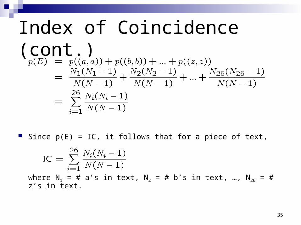
Index of Coincidence (cont.)

To compute p(E), we need to find the probability of each outcome in E. To do this, let

N = # letters in text N1 = # a’s in text N2 = # b’s in text … N26 = # z’s in text Using FPC and the fact that any pair of letters

has the same chance of being drawn, we find:

26


27


28


29


30


31


32


33


Since p(E) = IC, it follows that for a piece of text,

34



35



where N1 = # a’s in text, N2 = # b’s in text, …, N26 = # z’s in text.

36


Note that for a text with a large number of letters, N ≈ N-1 and N1 ≈ N1 -1, …, N26 ≈ N26-1. Therefore, for large amounts of text, we can use this

approximation to the IC:

37




38




Thus, IC ≈ sum of squares of relative frequencies of the letters a, b, …, z!

39

Example 4: Find IC of Each!

(a) English Language: Using the relative frequency table for the English language (see

handout or The Code Book—p. 19), IC ≈ (0.082)2 + (0.015)2 + (0.028)2 + … + (0.001)2 = 0.065 (b) A language in which each of 26 letters have the same

relative frequency: IC ≈ (1/26)2 + (1/26)2 + … + (1/26)2 = 1/26 = 0.038 (c) Any monoalphabetic cipher (in English): The frequency distribution of the letters is the same as that of the

English language, with the letters relabeled. Therefore IC ≈ 0.065.

40

Final Remarks on the Friedman Test Example 4 suggests that if a polyalphabetic

cipher is used, one will find an IC that is closer to 0.038, the case in which all 26 letters of the alphabet occur with the same frequency!

Using the IC on a piece of ciphertext to guess the type of cipher is the Friedman Test.

Another version of this test is used to find Vigenère cipher keyword lengths-see HW 2!

1 codes, ciphers, and cryptography-ch 2.3 michael a. karls ball state university

Documents

b experiment

c experiment

sample space s

e experiment

event e

d experiment

sample spaces

probability models