Continuing Professional Development

Version 2.0

A-level Computing

Stepping up to A2

Comparison of Algorithms

Permission to reproduce all copyright materials have been applied for. In some cases, efforts to contact copyright holders have been unsuccessful and AQA will be happy to rectify any omissions of acknowledgements in future documents if required.

COMPARISON OF ALGORITHMS ............................................................................................................2 SIZE OF INPUT ......................................................................................................................................................3 COMPLEXITY OF A PROBLEM ..................................................................................................................4 UNITS FOR MEASURING TIME .................................................................................................................4 ORDER OF GROWTH .......................................................................................................................................4 ASYMPTOTIC BEHAVIOUR ..........................................................................................................................5 BIG O NOTATION ................................................................................................................................................6 ORDER OF COMPLEXITY .............................................................................................................................7 LINEAR TIME ..........................................................................................................................................................7 POLYNOMIAL TIME ............................................................................................................................................7 EXPONENTIAL TIME .........................................................................................................................................7 COMPLEXITY OF SIMPLE LOOP .............................................................................................................8 ASSESSING ORDER OF GROWTH COMPLEXITY OF BLACK AND WHITE DISCS ...........................................................................................................................................................................8 TRACE TABLE FOR DISCS IN A ROW PROBLEM .......................................................................9 HOW TO DERIVE ORDER OF COMPLEXITY FROM PSEUDOCODE ...........................10 ORDER OF COMPLEXITY AND LINEAR SEARCH .....................................................................12 ORDER OF COMPLEXITY AND BUBBLE SORT ..........................................................................13 HOW AM I GOING TO TEACH THIS SECTION? ...........................................................................14 SPECIMEN QUESTION AND ANSWERS ON THIS SECTION .............................................15 COMMENT FROM CHIEF EXAMINER ON SCOPE OF BIG ‘O’QUESTIONS .............15 BIBLIOGRAPHY ..................................................................................................................................................16

COMPARISON OF ALGORITHMS

As our students know from studying COMP1 in the AS course, an algorithm is a set of unambiguous instructions for solving a problem. In simple terms, algorithms are used to transform inputs into outputs. A computer may or may not be involved. The main focus of this section of the specification is to answer the question “How long does it take for a machine to compute an output for a given input”? Frequently in computing, there are several ways to write an algorithm to solve a problem. We are all familiar with the concept of different sort routines. Students are aware of Bubble Sorts at AS level and will meet other sorts in A2 such as the Insertion Sort. Probably, it is best to introduce this idea in the way that the Nelson Thornes A2 textbook has done by considering two different methods for adding up the sequence of natural numbers i.e. 1, 2, .. 99, 100 represents the first hundred positive (non zero) natural numbers. Addition of natural numbers is the most basic arithmetic binary operation.

a + b = c

Here, a is the augend, b is the addend, and c is the sum.

As we know from primary school, we can simply add each number together and produce a running total which we then use as the augend for the next summation.

1 2 3 4 …. 99 100

1 + 2 = 3 3 + 3 = 6 etc

Writing the Algorithm in pseudocode we get: Sum 0 // initialise the running total For Count 1 to n // n is the largest number in the set Sum Sum + Count // add running total EndFor Output Sum

If you were to hand trace this algorithm for the first 10 non zero natural numbers, you get 55.

Nat Num 1 2 3 4 5 6 7 8 9 10

Running Total 3 6 10 15 21 28 36 45 55

2

However, mathematicians know that it can also be computed using the formula:

Sum = ½ n ( n + 1) which reassuringly still gives the answer of 55. The pseudocode is simply:

sum n * (n + 1) / 2 // compute sum of numbers Output Sum You could get your students to code these two different ways of ‘computing the sum’ into their preferred programming language and then run it to prove that you get the same answer. If you declare your integers to be large values, you may be able to output the elapsed times for both methods. There will be a Delphi solution in the NT online resources. If you know your processor speed, you will be able to estimate the time for any value of n as in the textbook. This simple example shows that algorithms for the same problem can be based on completely different approaches and can solve the problem with dramatically differing speeds. In all cases, we need to ensure that an algorithm produces the correct output for all valid inputs and not just some of them. Correctness is just part of the consideration about how good an algorithm is. The amount of memory used and the speed of computation for a given set of values are also important. Computational complexity theory is a branch of the theory of computation in Computer Science that investigates the problems related to the resources required to run algorithms, and the inherent difficulty in providing algorithms that are efficient for both general and specific computational problems. The computational complexity depends on both the space complexity and the time complexity. The problem now is that we are all used to microcomputers with very fast processors and vast amounts of RAM. This was not true in the early ‘80s!!

Time complexity - indicates how fast it runs

Space Complexity - indicates how much memory space is needed. There is often a trade off between time and space. The A2 textbook has a good example involving a program to find the factors of a number. The solution suggested is efficient in space complexity but very wasteful in terms of time complexity. Again, students are encouraged to code this into their chosen programming language and then to incorporate timing calculations. There will be a Delphi solution in the online resources. I find that there is insufficient time during lessons for students to develop such solutions so I tend to set them for exercises at home before the next lesson.

SIZE OF INPUT Students will probably be aware from the standard algorithm section in COMP1 that the number of items to be searched or sorted will have a major impact on how long it takes to carry out the operation. It takes longer to do a linear search on 1000 items as compared to just 10. Consequently it is important to understand an algorithm’s time efficiency in terms of the input size.

3

The A2 textbook considers the operation of reversing the elements of a list of 10 numbers compared with 1000.

COMPLEXITY OF A PROBLEM To compare algorithms for a particular task you have to consider the worst case complexity e.g. for a search of 100 items, you need to consider the case that the criteria match is the last item in the list not the first. Thus, the complexity of a problem is taken to be the worst case complexity for the most efficient algorithm that solves the problem. A common approach to computational complexity is the worst-case analysis; the estimation of the largest amount of computational resources (time or space) needed to run an algorithm. In many cases, the worst-case estimates are rather too pessimistic to explain the good performance of some algorithm in real use on real input. To address this, other approaches have been sought, such as average-case analysis or smoothed analysis.

UNITS FOR MEASURING TIME It is clearly inappropriate to use the SI unit of time i.e. the second to estimate the running time of a computation coded in a high level programming language. Any estimate would need to be based upon:

The processor speed The quality of the program used to implement the algorithm How efficient the compiler was that converted the high level code into machine code

Hopefully any supercomputer would execute a program faster than on a laptop. The alternative approach would be to count the number of times each algorithmic operation happens. This may be very difficult to do, so another approach is to consider which part of the algorithm contributes to the total running time. This is called the basic operation.

ORDER OF GROWTH Order of growth simply assesses by what factor execution time increases when the size of the input is increased. Putting this very simply, if we want to find the sum of the first 100 non zero positive integers, how much longer does it take than to sum just the first 10? We might also want to ignore machine dependent factors. If an algorithm takes two seconds to execute on one machine for a given input, a simplistic way to get it to run in one second would be to use a machine that is twice as fast. There is a constant multiplicative factor relating the speed of an algorithm on one machine and its speed on another, which we will ignore in this trivial treatment. We are only interested in how fast an algorithm runs on large inputs, since even slow algorithms finish quickly with small inputs.

4

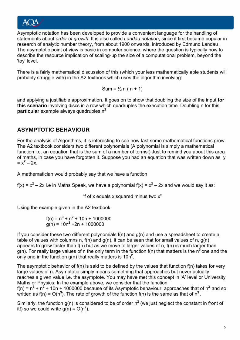
Asymptotic notation has been developed to provide a convenient language for the handling of statements about order of growth. It is also called Landau notation, since it first became popular in research of analytic number theory, from about 1900 onwards, introduced by Edmund Landau . The asymptotic point of view is basic in computer science, where the question is typically how to describe the resource implication of scaling-up the size of a computational problem, beyond the 'toy' level. There is a fairly mathematical discussion of this (which your less mathematically able students will probably struggle with) in the A2 textbook which uses the algorithm involving:

Sum = ½ n ( n + 1)

and applying a justifiable approximation. It goes on to show that doubling the size of the input for this scenario involving discs in a row which quadruples the execution time. Doubling n for this particular example always quadruples n2

ASYMPTOTIC BEHAVIOUR

For the analysis of Algorithms, it is interesting to see how fast some mathematical functions grow. The A2 textbook considers two different polynomials (A polynomial is simply a mathematical function i.e. an equation that is the sum of a number of terms.) Just to remind you about this area of maths, in case you have forgotten it. Suppose you had an equation that was written down as y = x2 – 2x. A mathematician would probably say that we have a function f(x) = x2 – 2x i.e in Maths Speak, we have a polynomial f(x) = x2 – 2x and we would say it as:

“f of x equals x squared minus two x”

Using the example given in the A2 textbook

f(n) = n3 + n2 + 10n + 1000000 g(n) = 10n2 +2n + 1000000

If you consider these two different polynomials f(n) and g(n) and use a spreadsheet to create a table of values with columns n, f(n) and g(n), it can be seen that for small values of n, g(n) appears to grow faster than f(n) but as we move to larger values of n, f(n) is much larger than g(n). For really large values of n the only term in the function f(n) that matters is the n3 one and the only one in the function g(n) that really matters is 10n2.

The asymptotic behavior of f(n) is said to be defined by the values that function f(n) takes for very large values of n. Asymptotic simply means something that approaches but never actually reaches a given value i.e. the asymptote. You may have met this concept in ‘A’ level or University Maths or Physics. In the example above, we consider that the function f(n) = n3 + n2 + 10n + 1000000 because of its Asymptotic behaviour, approaches that of n3 and so written as f(n) = O(n3). The rate of growth of the function f(n) is the same as that of n3 .

Similarly, the function g(n) is considered to be of order n2 (we just neglect the constant in front of it!) so we could write g(n) = O(n2).

5

For large values of n, it is the functions order of growth that matters. There are several functions that are especially important in the analysis of algorithms.

BIG O NOTATION Definition: A theoretical measure of the execution of an algorithm, usually the time or memory needed, given the problem size n, which is usually the number of items. ‘In Maths and Computer Science, big O notation describes the limiting behavior of a function when the argument tends towards a particular value or infinity, usually in terms of simpler functions. Big O notation allows its users to simplify functions in order to concentrate on their growth rates: different functions with the same growth rate e.g. O(n2) may be represented using the same O notation.’ Although originally developed as a part of pure mathematics, this notation is now frequently also used in computational complexity theory to describe an algorithm's usage of computational resources. The worst case or average case running time or memory usage of an algorithm is often expressed as a function of the length of its input (i.e. how many input values) using big O notation. This allows algorithm designers to predict the behaviour of their algorithms and to determine which of multiple algorithms to use, in a way that is independent of computer architecture or clock rate. Just to complicate matters and to recognise the theoretical work by different people, Big O notation is also called Big Oh notation, Landau notation, Bachmann–Landau notation, and Asymptotic Notation. Some of the classes of functions that are often found when analysing algorithms are listed in the table below. The importance of this measure can be seen in trying to decide whether an algorithm is adequate, but may just need a better implementation, or the algorithm will always be too slow on a big enough input. For example a quicksort which is O(n log n) on average (it is actually O(n2) in the worst case scenario), running on a small desktop computer can beat a bubble sort which is O(n²), running on a supercomputer if there are a lot of numbers to sort. To sort 1,000,000 numbers, the quicksort takes 20,000,000 steps on average, while the bubble sort takes 1,000,000,000,000 steps! See Jon Bentley, Programming Pearls: Algorithm Design Techniques, CACM, 27(9):868, September 1984 for an example of a microcomputer running BASIC beating a supercomputer running FORTRAN. The least complex is sometimes written as f = O(n0) i.e O(1) since any number to the power zero is 1.

Notation Name Example O(1) Constant Determining if a number is even or odd; using a constant-

size lookup table or hash table O(log2 n) Logarithmic Finding an item in a sorted array with a binary search O(n) Linear Finding an item in an unsorted list; adding two n-digit

numbers O(n log2 n) Linearithmic Performing a Fast Fourier transform; heapsort, or merge

sort or quicksort in the average case

6

O(n2) Quadratic Multiplying two n-digit numbers by a simple algorithm; adding two n×n matrices; bubble sort, shell sort, quicksort (in the worst case), or insertion sort

O(n3) Cubic Multiplying two n×n matrices by simple algorithm; finding the shortest path on a weighted digraph with the Floyd-Warshall algorithm; inverting a (dense) nxn matrix

O(2n) Exponential or Geometric

Finding the (exact) solution to the travelling salesman problem using dynamic programming; determining if two logical statements are equivalent using brute force

O(n!) Factorial Solving the travelling salesman problem via brute-force search

ORDER OF COMPLEXITY The complexity of a problem is considered to be the growth rate of the most efficient algorithm which solves the problem. We usually express it by stating the order of growth in big O notation. This is known as the order of complexity. The table above adapted from the Wikipedia article that I have used extensively in these notes allows us to rank an algorithm’s order of complexity.

O(n0) << O(n2) << O(n!)

LINEAR TIME A linear time algorithm is an algorithm that executes in O(n) time. Typically, this is exemplified by the algorithm used to find an item in an unsorted list or adding two n-digit numbers together. It is a special case of the polynomial type discussed next.

POLYNOMIAL TIME The simplest examples of polynomials are equations like f(n) = n2 or f(n) = n3 etc. Polynomial growth simply means that the equation has the form of f(n) = na where a might be 2 or 3 and n takes the values 1, 2, 3 etc. A polynomial time algorithm is one whose execution time grows as a polynomial of the size of input values.

EXPONENTIAL TIME Growth rates of the form 2n or 3n or in general kn where k is a constant are known as exponential growth rates and algorithms in this class are described as exponential time algorithms.

Increasing Order of Complexity

7

For large values of n, exponential growth rates far exceed polynomial growth rates. If n increases by a factor of 10, n2 will increase by a factor of 100 whereas 2n increases by a factor of approximately 1030.

COMPLEXITY OF SIMPLE LOOP

n 10 // Assignment not reliant on actual value of n

Print n // Execution not reliant on actual value of n

For i 1 to n

Print i // loop code block executes n times

EndFor

Print “Finished” // Execution not reliant on actual value of n

In this very simple piece of pseudocode, the only code block that takes longer as the size of the array grows is the loop. Therefore, the assignment statement and the two print statements outside of the loop are said to have a constant time complexity, or O(1), because they don't rely on n. The loop itself has a number of iterations equal to the size of the loop counter, so we can say that the loop has a linear time complexity, or O(N) in big ‘O’ notation.

The entire pseudocode stub has a time complexity of 3 * O(1) + O(N), and because constants e.g. 3 are removed, it is simplified to O(1) + O(N). Asymptotic notation also typically ignores the terms that grow more slowly because eventually the term that grows more quickly will dominate the time complexity as n moves toward infinity. So by ignoring the constant time complexity because it grows more slowly than the linear time complexity, we can simplify the asymptotic bound of the function to O(N). Hence the conclusion is that this particular pseudocode stub has linear time complexity. If we say that a function is O(N) then if n doubles, the algorithm’s time complexity at most will double. It may sometimes be less for other algorithms, but never more.

ASSESSING ORDER OF GROWTH COMPLEXITY OF BLACK AND WHITE DISCS You will recognize this example from the A2 textbook. It requires the rearrangement of a line of discs consisting of an equal number of black and white discs so that the black discs end up on the right in one group and the white discs end up on the left in another group. For example, two black discs followed by two white discs become two white discs followed by two black discs, as shown below. Here is a general algorithm for rearranging a line of discs containing an equal number of black and white discs for which the total number of discs greater than or equal to 2:

8

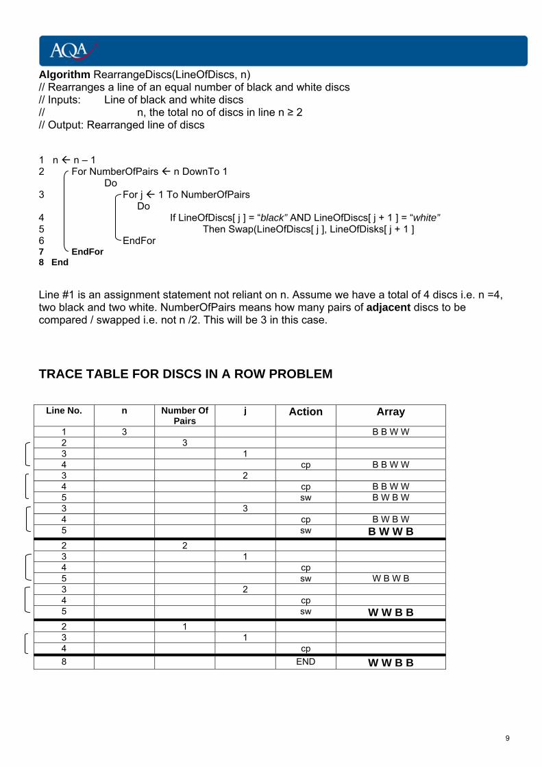
Algorithm RearrangeDiscs(LineOfDiscs, n) // Rearranges a line of an equal number of black and white discs // Inputs: Line of black and white discs // n, the total no of discs in line n ≥ 2 // Output: Rearranged line of discs 1 n n – 1 2 For NumberOfPairs n DownTo 1 Do 3 For j 1 To NumberOfPairs Do 4 If LineOfDiscs[ j ] = “black” AND LineOfDiscs[ j + 1 ] = “white” 5 Then Swap(LineOfDiscs[ j ], LineOfDisks[ j + 1 ] 6 EndFor 7 EndFor 8 End Line #1 is an assignment statement not reliant on n. Assume we have a total of 4 discs i.e. n =4, two black and two white. NumberOfPairs means how many pairs of adjacent discs to be compared / swapped i.e. not n /2. This will be 3 in this case.

TRACE TABLE FOR DISCS IN A ROW PROBLEM

Line No. n Number Of Pairs

j Action Array

1 3 B B W W 2 3 3 1 4 cp B B W W 3 2 4 cp B B W W 5 sw B W B W 3 3 4 cp B W B W 5 sw B W W B 2 2 3 1 4 cp 5 sw W B W B 3 2 4 cp 5 sw W W B B 2 1 3 1 4 cp

8 END W W B B

9

The basic operation for this algorithm is the comparison:

If LineOfDiscs[ j ] = black And LineOfDiscs[ j + 1] = white.

The number of comparisons is 3 when NumberOfPairs = 3,

it is 2 when NumberOfPairs = 2 and

1 when NumberOfPairs = 1

Therefore the total number of comparisons is 1 + 2 + 3 i.e. the sum of the first n – 1 natural numbers for this case with n=4. We know from earlier that the sum of the first m natural numbers is m so we can obtain the sum of the first n - 1 natural numbers by writing m = n - 1, which gives This result also applies if n is 2, 3, 4, 5, 6 or any natural number greater than 6 (but n can only be an even number for this particular example). We can expand this formula to obtain: And for large values of n, we get: This means that the order of growth of this algorithm is O (n2), i.e. “Order of n squared”

HOW TO DERIVE ORDER OF COMPLEXITY FROM PSEUDOCODE O(1) - constant time complexity This means that the algorithm requires the same fixed number of steps regardless of the size of the task e.g.

1) A single statement involving basic operations Here are some examples of basic operations:

One assignment (e.g. x:= 1 One arithmetic operation (eg., +, *) One test (eg., If x = 0) One read (accessing an element from an array)

2) A sequence of statements involving basic operations.

statement 1; statement 2; .......... statement k;

2

nn 1)(n n

2

1 2

1)(n n2

1

22

n2

nn

10

The time to execute each statement in the block is constant and so the total time is also constant even if it is 5 * O(1) if there are 5 simple statements, hence it is O(1) O(N) - Order of N i.e. linear time complexity This means that the algorithm requires a number of steps proportional to the size of the task e.g.

1. Stepping through an array. 2. Sequential / Linear search in an array. 3. Best case time complexity of Bubble sort (i.e when the elements of array are in

sorted order). Basic structure is :

For i 1 to n Do

A sequence of statements each of O(1) EndFor The loop executes n times, so the total time is n * O(1) which is O(N).

2O(N ) - Order of N Squared or quadratic time The number of operations is proportional to the size of the task squared e.g. Worst case time complexity for Bubble, Selection and Insertion sort.

Nested loops: 1. e.g. filling up a 2-D array

For i 1to r For j 1 to c

Do A sequence of assignment statements each of O(1)

EndFor EndFor

The outer loop executes n times and inner loop executes m times so the time complexity becomes O(r * c) which is effectively an example of O(n2) 2.

For i = 1 to n For j = 1 to n

Do A sequence of statements of O(1)

EndFor EndFor

Both inner and outer loops execute n times. Now the time complexity is O(n2)

11

O(log n) logarithmic time complexity e.g. Binary search in a sorted array of n elements. O(n log n) "n log n " time complexity e.g. MergeSort, QuickSort etc. where (a>1), Order of a to power of n - exponential time e.g.

1. Recursive Fibonacci series implementation 2. Towers of Hanoi

The ‘best’ time complexity in the above list is obviously constant time, and the ‘worst’ is exponential time which, as we have seen, quickly overwhelms even the fastest computers even for relatively small n. Polynomial growth (linear, quadratic, cubic, etc.) is considered manageable as compared to exponential growth.

ORDER OF COMPLEXITY AND LINEAR SEARCH

Suppose n = 5 and consider the worst case scenario where the target value is in the last array position. Array Value Operation

1 cp 2 cp 3 cp 4 cp 5 cp

To see if there is a match, there have been a total of n comparisons. Suppose the time for a comparison is represented by C, then the time to search all of the elements has been:

n * C but C is a constant for a particular system

Hence T = O (n) for a linear search

12

ORDER OF COMPLEXITY AND BUBBLE SORT Suppose n = 5 and consider the very worst case scenario where the list is in reverse order. Value OP Value OP Value OP Value OP Value OP 5 4 3 2 1 cp +

sw cp +

sw cp +

sw cp +

sw cp only

4 3 2 1 2 cp +

sw cp +

sw cp +

sw cp only cp only

3 2 1 3 3 cp +

sw cp +

sw cp only cp only cp only

2 1 4 4 4 cp +

sw cp only cp only cp only cp only

1 5 5 5 5 = 4 * (cp + sw) = 3 * (cp + sw) = 2 * (cp +sw) = 1 * (cp + sw) = 0 * (cp + sw)

= (n-1)*(cp+sw) = (n-2)*(cp+sw) = (n-3)*(cp+sw) =(n-4)*(cp+sw) =(n-5)*(cp+sw) + 0 * cp + 1 * cp + 2 * cp + 3 * cp + 4 * cp

Suppose we represent the time for a compare (cp) plus a swap (sw) operation as A and the time for just a compare (cp) operation as B. The total time T in this case with just 5 items is thus:

(n-1)*A + (n-2)*A + (n-3)*A + (n-4)*A + 1 * B +2 * B + 3 * B + 4 * B In general, it equals: A * (( n - 1) + ( n - 2) + ………..+ 1) + B * ((1 + 2 + 3 + …………(n – 1))

= t = n - 1 t = n - 1

t = 1 t = 1

A * t + B * t

= t = n - 1

t = 1

(A + B) t

However, Gauss proved at the age of 8!!! that r = m

r = 1

m (m + 1)r =

2 (Triangular numbers or sum of natural

numbers) And m = n - 1 (by comparing the two upper summation limits

=(n - 1) (n - 1 + 1)

(A + B)2

This simplifies to:

For really large values of n, we can ignore the term in n so this in turn simplifies to 2 n

(A + B)2

The term (A + B) is a constant for a given system so for really, really large values of n, our expression approximates further and we can ignore the denominator. Thus the order of complexity for our Bubble Sort becomes:

T 2= O (n )

2(n - n)(A + B)

2

13

HOW AM I GOING TO TEACH THIS SECTION? If your candidates are taking A level pure maths or are at least mathematically competent, you can follow the approach in the A2 textbook with all of the equations and approximations etc, but if they only have achieved grade C at GCSE and are not taking any mathematical subjects in the Sixth Form, they may struggle. They need to grasp the key concepts for the Comparison of Algorithms that are listed in the specification namely:

Understand that algorithms can be compared by expressing their complexity as a function relative to the size of the problem.

Understand that some algorithms are more efficient time-wise than other algorithms. Understand that some algorithms are more space-efficient than other algorithms. Big-O notation Linear time, polynomial time, exponential time.

Algorithms are potentially a very mathematical topic and are treated as such in many University Computer Science courses. Simulation of various sort and search algorithms using varying values for input size should help reinforce these concepts especially for weaker students. Most of these are available as Java Applets and do not need to be downloaded onto workstations. Some URLs are given at the end of the Bibliography.

14

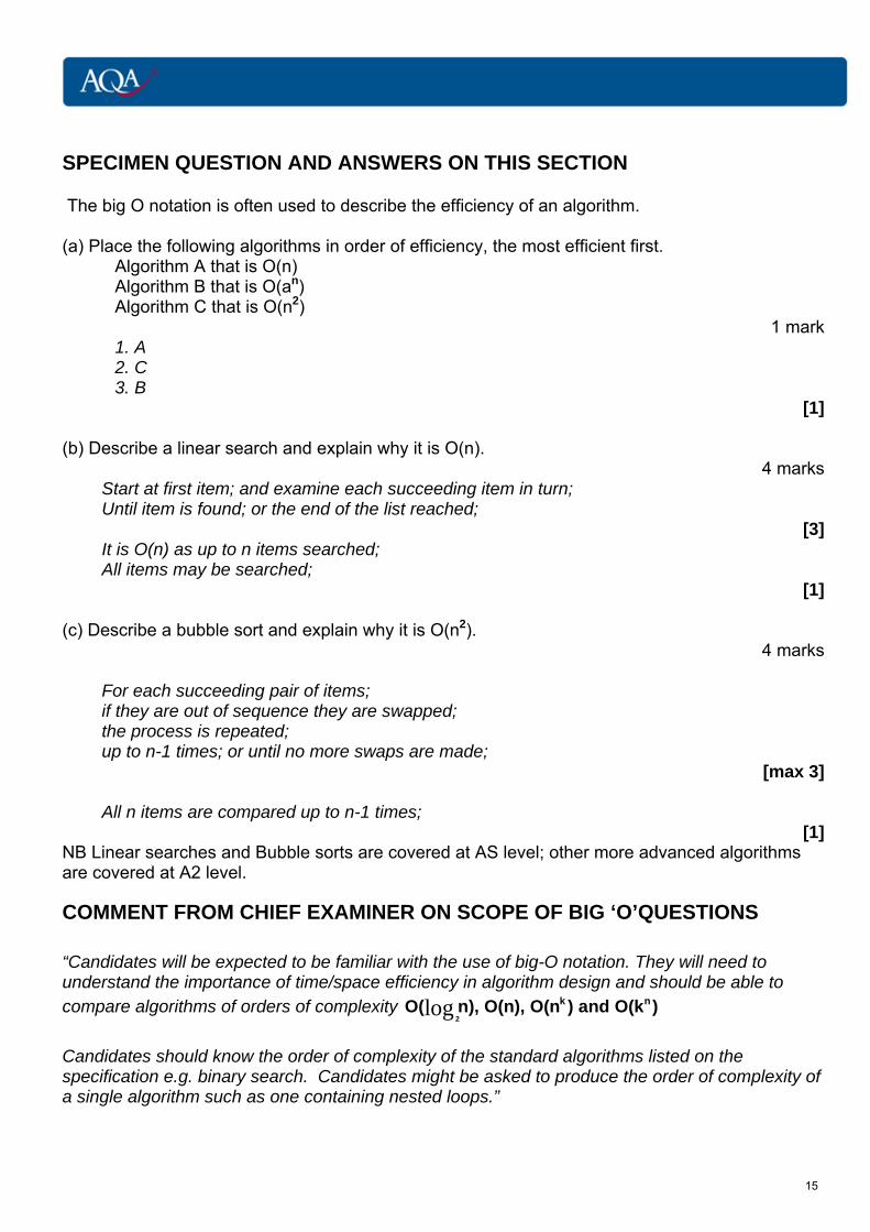
SPECIMEN QUESTION AND ANSWERS ON THIS SECTION The big O notation is often used to describe the efficiency of an algorithm. (a) Place the following algorithms in order of efficiency, the most efficient first.

Algorithm A that is O(n) Algorithm B that is O(an) Algorithm C that is O(n2)

1 mark 1. A 2. C 3. B

[1] (b) Describe a linear search and explain why it is O(n).

4 marks Start at first item; and examine each succeeding item in turn; Until item is found; or the end of the list reached;

[3] It is O(n) as up to n items searched; All items may be searched;

[1] (c) Describe a bubble sort and explain why it is O(n2).

4 marks

For each succeeding pair of items; if they are out of sequence they are swapped; the process is repeated; up to n-1 times; or until no more swaps are made;

[max 3]

All n items are compared up to n-1 times; [1]

NB Linear searches and Bubble sorts are covered at AS level; other more advanced algorithms are covered at A2 level.

COMMENT FROM CHIEF EXAMINER ON SCOPE OF BIG ‘O’QUESTIONS “Candidates will be expected to be familiar with the use of big-O notation. They will need to understand the importance of time/space efficiency in algorithm design and should be able to compare algorithms of orders of complexity log

2

k nO( n), O(n), O(n ) and O(k )

Candidates should know the order of complexity of the standard algorithms listed on the specification e.g. binary search. Candidates might be asked to produce the order of complexity of a single algorithm such as one containing nested loops.”

15

BIBLIOGRAPHY 'AQA Computing A2' by Kevin Bond and Sylvia Langfield, published by Nelson Thornes ISBN 978-0-7487-8296-3 'AQA Computing AS' by Kevin Bond and Sylvia Langfield, published by Nelson Thornes ISBN 978-0-7487-8298-7 http://en.wikipedia.org/wiki/Addition_of_natural_numbers http://www.9math.com/book/sum-first-n-natural-numbers - proof of Sum = ½ n ( n + 1) http://en.wikipedia.org/wiki/Computational_complexity_theory http://courses.washington.edu/tcss343/slides/BigOhBruteForceDivideConq.pdf http://www.cs.berkeley.edu/~kamil/teaching/fa02/100302.pdf http://en.wikipedia.org/wiki/Asymptotic_analysis Algorithms: design techniques and analysis By M. H. Alsuwaiyel Published by World Scientific, 1998 ISBN 9810237405, 9789810237400 http://people.csail.mit.edu/devadas/6.001/rec4.pdf http://www.cs.uwaterloo.ca/%7Ealopez-o/comp-faq/faq.html (Computational models and complexity) http://nvl.nist.gov/pub/nistpubs/sp958-lide/html/140-144.html (General paper on Algorithms) http://en.wikipedia.org/wiki/Big_O_notation http://www.itl.nist.gov/div897/sqg/dads/HTML/bigOnotation.html http://en.wikipedia.org/wiki/Analysis_of_algorithms http://www.csanimated.com/animation.php?t=Big_O_notation http://www.cs.helsinki.fi/research/aaps/excel/download/bubble7.bin http://www.cs.helsinki.fi/research/aaps/excel/ http://courses.cs.vt.edu/%7Ecs1104/FrontEnd/index.html or http://courses.cs.vt.edu/~csonline/ Definition and specification of algorithms, with a comparison and analysis of several sorting algorithms as examples. http://www.iitk.ac.in/esc101/2009Jan/lecturenotes/timecomplexity/TimeComplexity_using_Big_O.pdf

16

http://www.progressive-coding.com/tutorial.php?id=1 - linear_search http://rob-bell.net/2009/06/a-beginners-guide-to-big-o-notation/ http://delicious.com/nstoneit/bigo http://www.sparknotes.com/cs/searching/efficiency/summary.html http://echochamber.me/viewtopic.php?f=12&t=38742 http://www.academicearth.org/lectures/run-times-and-algorithms-recu...

17