1

Density-based Place Clustering UsingGeo-Social Network Data

Dingming Wu, Jieming Shi, and Nikos Mamoulis,

Abstract—Spatial clustering deals with the unsupervised grouping of places into clusters and finds important applications in urbanplanning and marketing. Current spatial clustering models disregard information about the people and the time who and when arerelated to the clustered places. In this paper, we show how the density-based clustering paradigm can be extended to apply on placeswhich are visited by users of a geo-social network. Our model considers spatio-temporal information and the social relationshipsbetween users who visit the clustered places. After formally defining the model and the distance measure it relies on, we providealternatives to our model and the distance measure. We evaluate the effectiveness of our model via a case study on real data; inaddition, we design two quantitative measures, called social entropy and community score to evaluate the quality of the discoveredclusters. The results show that temporal-geo-social clusters have special properties and cannot be found by applying simple spatialclustering approaches and other alternatives.

Index Terms—Clustering, Similarity Measurements, Algorithms.

F

1 INTRODUCTION

C LUSTERING is commonly used as a method for data explo-ration, characterization, and summarization. Density-based

clustering [1], in particular, divides a large collection of points intodensely populated regions and it is the most appropriate clusteringparadigm for spatial data, which have low dimensionality [2].Density-based clusters have arbitrary shapes and sizes and excludeobjects in areas of low density (i.e., outliers). The DBSCAN model[1] finds the spatial eps-neighborhood of each point p in thedataset, which is a circular region centered at p with radius eps.If the eps-neighborhood of p is dense, meaning that it containsno less than MinPts places, p is called a core point. Dense eps-neighborhoods are put into the same cluster if they contain thecores of each other.

In this paper, we investigate the extension of traditionaldensity-based clustering for spatial locations to consider theirrelationship to a social network of people who visit them and thetime when they were visited. In specific, we consider the placesof a Geo-Social Network (GeoSN) application, which allowsusers to capture their geographic locations and share them inthe social network, by an operation called checkin. Online socialnetworks with this functionality include Gowalla1, Foursquare2,and Facebook Places3. A checkin is a triplet ⟨uid ,pid , time⟩modeling the fact that user uid visited place pid at a certain time .

We define the new problem of Density-based Clustering Placesin Geo-Social Networks (DCPGS), to detect geo-social clusters inGeoSNs. DCPGS extends DBSCAN by replacing the Euclidean

D. Wu is with the College of Computer Science & Engineering, ShenzhenUniversity, China.E-mail: dingming@szu.edu.cn

J. Shi (corresponding author) is with the Lenovo Big Data Lab, Hong KongE-mail: jshi@lenovo.com

N. Mamoulis is with the Department of Computer Science and Engineer-ing, University of Ioannina.E-mail: nikos@cs.uoi.gr

Manuscript received 2016; revised .1. http://gowalla.com2. https://foursquare.com3. https://www.facebook.com/about/location

distance threshold eps for the extents of dense regions by a thresh-old ε, which considers both the spatial and the social distancesbetween places. For two places pi and pj , the spatial distanceis considered to be the Euclidean distance between pi and pj ,while the social distance should consider the social relationshipsbetween the two sets of users Upi and Upj which have checked inpi and pj , respectively. We define and use such a social distancemeasure, based on the intuition that two places are socially similarif they share many common users in their checkin records or theusers in these records are linked by friendship edges. Figure 1(a)illustrates the data of a GeoSN that includes eight users (u1–u8) and two places (pi and pj). The dashed lines represent userfriendships and the solid lines annotated with timestamps (t1–t9)illustrate checkins of users at places. For instance, user u1 is afriend with u2 and u3 and has visited place pi at time t3 and pjat t5. As Figure 1(b) shows, each place is modeled by its spatialcoordinates (e.g., ⟨lai, loi⟩ for the latitude and longitude of pi)and the set of users that have visited it (e.g., Upi for pi). Forthe spatial distance between pi and pj , we can use the Euclideandistance between ⟨lai, loi⟩ and ⟨laj , loj⟩, while for the socialdistance component we use the set of common users in Upi andUpj (e.g., u1, u2) and the users in one place’s record who arefriends with visitors of the other place (e.g., u3 ∈ Upi and u6 ∈ Upjwho are friends with each other). The intuition is that users whoare friends can influence each other to visit the places includedin their checkin history. The details of our distance measure arepresented in Section 2.

In our previous work [3], the time of the check-ins made byusers is not considered during the clustering process. The socialconnections established between places may be either out-datedor based on distant checkins in terms of time. For instance, theplace clusters discovered according to the checkins one year agomay not interest analysts that value recent relationships betweenplaces. In addition, a cluster may have low quality if the check-in times of the different places in it vary significantly. In thispaper, we investigate three methods of incorporating the temporalinformation (i.e., when did users checkin at the various places)

2

u4

u8

u7

u6

u5

u2u1

u3

pjpi

t3

t1 t2

t4 t5t6 t7

t8t9

(a) A toy example

u4

u3

u2u1

u6

u5

u2

u1

u7

Upi

u8

Upj

pi : <lai, loi> pj : <laj, loj>

(b) Abstraction

Fig. 1. Example and storage structure of GeoSNs

in the process of geo-social clustering, i.e., (1) history-frame geo-social clustering, (2) damping window, and (3) temporally con-tributing users, yielding temporal-geo-social clusters. The threemethods of incorporating temporal information result in differentclusters that satisfy different analysis needs. The history-framemethod reveals how clusters evolve over time; its result can beused to analyze relationships between places at different periods oftime. The damping window method weighs the recently checkinshigher than old ones, so it generates clusters relevant to the currenttime. The temporally contributing user method only considersthe checkins that have been made within a period of time, andignores distant checkins. Hence, the places in the same cluster arevisited by socially related users in the same periods of time, whichindicates a stronger relationship between them. We compare thetemporal-geo-social clusters and the geo-social clusters based onvisualization and social entropy evaluation. The result shows thatthe temporal information helps improving the quality of clusters.

To the best of our knowledge, there is no previous work onclustering GeoSN places. While there exists a significant body ofresearch on analyzing and querying GeoSN data [4], [5], [6], [7],most of these works are centered around users; i.e., they studyuser behavior, user link prediction or recommendation, or theevaluation of user queries. Thus, the places and checkins are onlyregarded as some auxiliary information to facilitate user-centeredanalysis. On the other hand, GeoSNs provide a new and rich formof geographical data, affiliated with the social network graph,the analysis of which can provide new and interesting insights,compared to raw spatial data. In specific, clustering of places in aGeoSN network finds a number of interesting applications:Generalization and characterization of places. In geographicdata analysis, a common task is to define regions (especially inurban areas), which include similar places with respect to thepeople who live in them or visit them. For example, in urbanplanning, land managers are interested in identifying regionswhich have uniform (i.e., consistent) demographic statistics, e.g.,areas where elderly people prefer to visit, or people who belongto certain religious communities and have special transportationor living needs. Our DCPGS framework is especially useful forsuch spatial generalization and characterization tasks, because itcan identify geographic regions where places form dense regionsand the people who visit them are also socially connected to eachother. By considering also the temporal information in the data(i.e., when did users checkin at the various places), the discoveredclusters can be further refined and can become valuable for urbanactivity analysis, local authorities, service providers, decisionmakes, etc. For example, a certain set of places (e.g., shoppingspots) may be characterized as a cluster for only restricted timeperiods or intervals (e.g., during Saturday morning hours).Data cleaning. Intuitively, places that belong in the same geo-

social cluster, according to our DCPGS framework, should havesimilar semantics. Therefore, our clustering results can help to-ward the cleaning of semantics (e.g., tags), which are givento places being in the same cluster (e.g., inspect tags that areinconsistent with the ones given to the majority of places inthe cluster). In addition, as already mentioned, nearby GeoSNlocations collected by user checkins could belong to the samephysical place (e.g., a large restaurant) and our clusters can helptoward identifying such cases and integrating multiple locations tothe same physical place (i.e., region), possibly with the joint helpof map-matching tools. Besides, taking the temporal dimensioninto account can also help to provide more accurate cleaning.Marketing. GeoSN places may be commercial (e.g., restaurants).The fact that two (or more) such places belong to the samegeo-social cluster indicates that there is a high likelihood that auser who likes one place would also be interested to visit theother(s). Therefore, by having knowledge of a place’s geo-socialcluster, the management of the place may initiate campaigns tousers who visited other places in the same cluster, or a set ofplaces could do collaborative promotion (e.g., a discount for userswho visit multiple places in the cluster). In addition, the user-groups that are relevant to a cluster could be relative to certaintime periods. For example, shopping places in downtown arevisited during the evening by people who have to work andcould not shop at daytime, while supermarkets and small shopsin the suburbs are usually visited by housewives in the daytime.Such geo-social-temporal clusters can be useful to marketing oradvertising companies, which may benefit from understanding the(time sensitive) shopping habits of various social groups.

Compared to conventional density-based spatial clusters, geo-social clusters detected by DCPGS exhibit larger intra-cluster so-cial strength, as we confirm experimentally in Section 3. DCPGSalso has additional advantages. First, DCPGS uses geo-socialsplitting criteria; for example, DCPGS splits clusters, which arespatially dense, but they are separated by barriers, such as rivers orwalls, or visitors’ weak social connections. Second, DCPGS findsspatially loose clusters that include sets of places that (pairwise)are not very close to each other (and therefore violate a typicallytight spatial density threshold), but have very tight social relation-ships with each other. Such places satisfy our DCPGS criteria.On the other hand, DBSCAN is less flexible in including them inthe same cluster as loosening its spatial distance threshold wouldresult in putting everything in a single huge cluster. Third, DCPGScan discover geo-social clusters with fuzzy spatial boundaries;such clusters cannot be identified by spatial clustering, whichdefines strict spatial boundaries between clusters. Our evaluationis based on case studies and on the use of quantitative measuresthat we also propose in this paper. In addition, we demonstratethat the social distance measure we propose and use in DCPGSis more effective compared to alternative measures (based onnode-to-node proximity). Overall, the results of our evaluationindicate that the social relationships between users who visitplaces have great impact in the clustering of places and cannot beoverlooked. Furthermore, considering the temporal information inthe clustering not only reveals how the clusters evolve with time,but also helps finding groups of places having more coherent socialrelationships.

Summing up, the contributions of this paper are as follows:

We propose and formulate the problem of density-basedclustering GeoSN places.

3

We define a simple but effective social distance measurebetween places in GeoSNs.

We demonstrate the effectiveness of DCPGS by case studiesand quantitative evaluation through two quality measures thatare also devised in this paper.

We study three ways of incorporating temporal informationin DCPGS and evaluate the resulting temporal-geo-socialclusters.

The rest of the paper is organized as follows. Section 2 for-mulates the DCPGS problem, defines the social distance measurebetween places that we use, and introduces three methods of in-corporating temporal information into DCPGS. The effectivenessof our framework are analyzed in Sections 3. Related work isreviewed in Section 4. Finally, Section 5 concludes this paper anddiscusses future work. The efficient algorithms in our previouswork [3] for clustering GeoSN places and the performance evalu-ations are presented in Appendices B and C.

2 MODEL AND DEFINITIONS

Our data input includes three components: a social network, aset of places and the checkins of users to the places. The socialnetwork is an undirected graph G = (U,E), where U is the set ofall users and each edge (ui, uj) ∈ E indicates that users ui, uj ∈U are friends. Set P is the set of all places visited by users, inthe form of ⟨latitude, longitude⟩ GPS points. Thus, identifiers areassigned to places according to their distinct GPS coordinates. SetCK = ⟨ui, pk, tr⟩∣ui ∈ U and pk ∈ P includes all checkinsgenerated by users in U . A checkin in CK is a triplet ⟨ui, pk, tr⟩modelling the fact that user ui visited place pk at a certain tr .For a place pk, the set Upk of visiting users of pk is defined byUpk = ui∣⟨ui, pk,∗⟩ ∈ CK, where ∗ means any time. Figure1(b) shows Upi and Upj for the two places pi and pj of the toyexample in Figure 1(a). The figure also connects the user pairsin the two sets who are linked by friendship edges in the socialnetwork. Note that user u8 does not belong to either Upi or Upj ,but connects users u4 and u7 in the social graph.

2.1 DCPGS Model

Our Density-based Clustering Places in Geo-Social Networks(DCPGS) model extends the model of DBSCAN [1]; foreach place pi in the GeoSN, DCPGS finds the geo-social ε-neighborhood Nε(pi) of pi, which includes all places pjsuch that Dgs(pi, pj) ≤ ε, DS(pi, pj) ≤ τ , and E(pi, pj) ≤

maxD . For two places pi, pj , E(pi, pj) is the Euclidean dis-tance, DS(pi, pj) is the social distance, and Dgs(pi, pj) =

f(DS(pi, pj),E(pi, pj)) is the geo-social distance, defined asa function of E(pi, pj) and DS(pi, pj). Parameter ε is geo-social distance threshold, while τ and maxD are two sanityconstraints for the social and the spatial distances between places,respectively. We will give detailed definitions for all above dis-tance functions and parameters later on. If the geo-social ε-neighborhood of a place pi contains at least MinPts places, thenpi is a core place. In DCPGS, w.r.t. ε and MinPts ; a place pi isdirectly density-reachable from a place pj if pi ∈ Nε(pj) andNε(pj) ≥ MinPts ; a place pi is density reachable from a placepj if there is a chain of places p1,⋯, pn, p1 = pi, pn = pj suchthat pk−1 is directly density-reachable from pk (1 < k ≤ n); aplace pi is density connected to a place pj if there is a place pk,such that both pi and pj are density-reachable from pk. A cluster

C in DCPGS w.r.t. ε and MinPts is a non-empty subset of placessatisfying the following conditions: 1) ∀pi, pj : if pi ∈ C and pjis density-reachable from pi then pj ∈ C . 2) ∀pi, pj ∈ C: pi isdensity-connected to pj . Outliers are the places that do not belongto any cluster.Parameters. ε and MinPts are the main parameters of DCPGS.MinPts (i.e., the minimum number of places in the neighborhoodof a core point) is set as in the original DBSCAN model (see [1]);a typical value is 5. ε takes a value between 0 and 1, because, as weexplain later on, we defineDgs(pi, pj) to take values in this range.Since the geo-social distance Dgs(pi, pj) is a function of a spatialand a social distance, τ and maxD constrain these individualdistances to avoid the following two cases that negatively affectthe quality of geo-social clusters.

The geo-social distance between two places pi and pj couldbe less than ε if they are extremely close to each other inspace, but have no social connection at all. This may leadto putting places close to each other spatially, but having nosocial relationship, into the same cluster.

The geo-social distance between two places pi and pj couldbe less than ε if they have very small social distance, but theyare extremely far from each other spatially. This may leadto putting places with close social distances, but large spatialdistances, into the same cluster.

Constraints τ and maxD are defined for quality control and canbe set by experts or according to the analyst’s experience. Weexperimentally study how clustering quality is affected by the twoconstraints and ε in Section 3.Distance Functions. The social distance DS(pi, pj) takes asinputs the sets of users Upi and Upj who have visited pi and pj ,respectively, and returns a value between 0 and 1. In Section 2.2,we present our definition for DS(pi, pj) and alternative waysto define it based on previous work. Before defining the geo-social distance Dgs(pi, pj), we convert the Euclidean distanceE(pi, pj) into a spatial distance DP (pi, pj) =

E(pi,pj)maxD so that

any place pj in the geo-social ε-neighborhood of pi has spatialdistance no larger than 1. Finally, Dgs(pi, pj) is defined asweighted sum of DS(pi, pj) and DP (pi, pj), i.e.,

Dgs(pi, pj) = ω ⋅DP (pi, pj) + (1 − ω) ⋅DS(pi, pj), (1)

where ω ∈ [0,1].

2.1.1 Alternatives to DCPGSUsing the proposed geo-social distance, our place clustering model(DCPGS) extends density-based clustering in spatial databases.We next present two alternatives to DCPGS, which can be alsoused to cluster GeoSN places.SNN-based Clustering. The SNN clustering algorithm [8] isan improvement of DBSCAN that can find clusters of widelydiffering shapes, sizes, and densities. It first finds the k nearestneighbors of each data point and then redefines the similaritybetween pairs of points in terms of how many nearest neighborsthe two points share. Using this definition of similarity, the SNNalgorithm identifies core points and then builds clusters around thecore points as DBSCAN does.

We extend SNN to cluster places in the geo-social network asfollows. Firstly, the neighborhood of a place p in SNN is defined asNN (p) = q ∈ P ∧ q ≠ p∣E(p, q) ≤ maxD and DS(p, q) ≤ τ.Then, according to SNN, the similarity between two places piand pj is defined as the cardinality of the common places in

4

their neighborhood, i.e., Ssnn(pi, pj) = ∣NN (pi) ∩ NN (pj)∣.Given a user specified similarity parameter epssnn , the SNN geo-social neighborhood of a place pi is defined as Nsnn(pi) =

pj ∈ P ∣Ssnn(pi, pj) ≥ epssnn. Place pi is a core place if∣Nsnn(pi)∣ ≥MinPtssnn , where MinPtssnn is the user specifieddensity threshold. If two core places are within each other’s SNNgeo-social neighborhood, then they are put into the same cluster.Graph-based Clustering. GeoSN places can alternatively beclustered by the use of graph clustering models. The main idea ofsuch a model is to construct a place network PN , which connectsplaces according to their social and spatial distances and thenapply an off-the-shelf community detection algorithm on PN .Specifically, given two places pi and pj , if E(pi, pj) ≤ maxDand DS(pi, pj) ≤ τ , an undirected and weighted edge with geo-social weight Wgs(pi, pj) = 1−Dgs(pi, pj) is added between piand pj . Community detection algorithms like Link Clustering [9],[10] or Metis [11] can then be applied to derive the clusters.Link Clustering constructs a dendrogram of network communities(that may overlap) in a hierarchical manner. Metis is anothermultilevel graph partition paradigm that includes three phases:graph coarsening, initial partitioning, and uncoarsening; Metisdivides a network into k non-overlapping communities. As wewill show in Section 3, these graph clustering methods are inferiorto DCPGS.

2.2 Social Distance Between PlacesThe social distance DS(pi, pj) between pi and pj naturallydepends on the social network relationships between the sets Upiand Upj of users who visited pi and pj , respectively. DS(pi, pj)is based on the set CU ij of contributing users between two placespi and pj :

Definition 1. (Contributing Users) Given two places pi and pjwith visiting users Upi and Upj , respectively, the set of contribut-ing users CU ij for the place pair (pi, pj) is defined as

CU ij = ua ∈ Upi ∣ua ∈ Upj or ∃ub ∈ Upj , (ua, ub) ∈ E

∪ ua ∈ Upj ∣ua ∈ Upi or ∃ub ∈ Upi , (ua, ub) ∈ E (2)

Specifically, if a user ua has visited both pi and pj , then ua isa contributing user. Also if ua has visited place pi, ub has visitedpj , and ua and ub are friends, both ua and ub are contributingusers. Users in CU ij contribute positively (negatively) to thesocial similarity (distance) between pi and pj . Formally:

Definition 2. (Social Distance) Given two places pi and pjwith visiting users Upi and Upj , respectively, the social distancebetween pi and pj is defined as

DS(pi, pj) = 1 −∣CU ij ∣

∣Upi ∪Upj ∣(3)

The above definition of DS(pi, pj) takes both the set sim-ilarity between sets Upi and Upj and the social relationshipsamong users in Upi and Upj into account. In addition, the distancemeasure penalizes pairs of places pi and pj which are popular(i.e., Upi and/or Upj are large) but their set of contributingusers is relatively small (see Equation 3). The reason is thatsuch place pairs are not characteristic to their (loose) socialconnections. As an example, consider places pi and pj of Figure1. To compute DS(pi, pj), we first set Upi = u1, u2, u3, u4and Upj = u1, u2, u5, u6, u7. All users in Upi and Upj arechecked one by one to obtain the contributing users between pi

and pj . We derive CU ij = u1, u2, u3, u5, u6, since (i) bothu1 and u2 have visited pi and pj , (ii) user u3, who visited pi,has a friend u6 who visited pj , (iii) symmetrically, user u6, whovisited pj , has a friend u3 who visited pi, and (iv) u5 (∈ Upj )has a friend u2 having been to pi. According to Definition 2,the social distance DS(pi, pj) between pi and pj in Figure 1 is1 − ∣CU ij ∣/(∣Upi ∪Upj ∣) = 1 − 5/7 ≈ 0.2857.

Observe that only direct friendship edges between users of Upiand Upj are considered in our social distance definition. Longernetwork paths, such as friend-of-friend relationships, are ignored(e.g., the case of users u4 and u7 in Figure 1(b) who are connectedvia user u8). According to the small world effect [12], a user ina social network can reach a large portion of other users withinonly few hops. For instance, the 90-percentile effective diameter[13] of Gowalla GeoSN, used in our experiments, is just 5.7.4 Thismeans within quite a few hops most users can reach a very largepercentage of all users. In Gowalla, only 8 users can access morethan 1% of all the users in 1 hop, while 40516 users (20.61%of all the users) can access more than 1% of all the users in 2hops and 141582 users (72.02% of all the users) can reach morethan 1% of all the users in 3 hops. The number of users who canreach more than 1% users in 2 or 3 hops increases dramaticallycompared to the percentage of those visited within 1 hop. Thus,paths longer than 1 hops are too common and cannot be consideredas (indirect) user relationships; i.e., their impact is much weakercompared to direct friendship edges. Hence, Definition 2 intro-duces a simple, but powerful social distance measure. Propertiesof DS(pi, pj) include symmetry (i.e., DS(pi, pj) = DS(pj , pi))and self-minimality (i.e., DS(pi, pj) ∈ [0,1], and DS(pi, pj) = 0for Upi = Upj ). On the other hand, DS(pi, pj) does not obeythe triangular inequality, but this does not affect our clusteringalgorithm.

2.2.1 Alternatives to DS

Our DCPGS model is independent of the social distance definitionbetween places (i.e., DS). As an alternative to our Definition 2,the following measures can be used. In Section 3, we evaluate theeffectiveness of these alternatives.Jaccard. Based on the Jaccard similarity J(pi, pj) = (∣Upi ∩Upj ∣)/(∣Upi ∪ Upj ∣) between the sets of visiting users for pi andpj , we define DJac

S (pi, pj) = 1−J(pi, pj), which is not intuitive;it disregards the social network, assuming that two users who arefriends do not affect each other in visiting GeoSN places.SimRank. SimRank is a structural-context model for measuringthe similarity between nodes in a graph. The idea is that twonodes are equivalent if they relate to equivalent nodes. We candefine a SimRank-based social distance Dsim

S (pi, pj), using theMinimax version of SimRank [14].5 This measure compares eachof pi’s visiting users upir with the visiting user upjs of pj who isthe most similar to upir , to compute the similarity between placess(pi, pj). The similarity between users s(upir , u

pjs ) is computed

in an analogous way. Specifically, DsimS (pi, pj) = 1 − s(pi, pj),

where s(pi, pj) = min(spi(pi, pj), spj(pi, pj)),spi(pi, pj) =

φ∣Upi

∣∑

ur∈Upi

maxus∈Upj

s(ur, us), where φ = 0.8 is a

decay factor [14], s(ur, us) = min(sur(ur, us), sus(ur, us)),

4. http://snap.stanford.edu/data/index.html5. The original SimRank measure is only meant for node-to-node similarity;

in our case, we need a measure between Upi and Upj .

5

and assuming that Pur is the set of places visited by ur,sur(ur, us) =

φ∣Pur ∣

∑pi∈Pur

maxpj∈Pus

s(pi, pj).

Katz. The Katz similarity measure [15] sums over all possiblepaths from user ur to us with exponential damping by length, i.e.,

K(ur, us) =∞

∑l=1βl∣paths lur,us

∣, where paths lur,usis the set of all

length-l paths from ur to us, and damping factor β is typicallyset to 0.05. Due to the poor scalability of this measurement, inpractice only paths up to length L are considered [16]; i.e., an

approximated Katz score Ka(ur, us) =L

∑l=1βl∣paths lur,us

∣ can be

used. Accordingly, we can define a Katz-based social distancebetween places pi and pj , by averaging the normalized Katzsimilarities between all pairs of users from Upi and Upj :

DKatzS (pi, pj) = 1 −

1

∣Upi ∣∣Upj ∣∑

ur∈Upi

∑us∈Upj

Ka(ur, us)

CommuteTime. The hitting time h(ur, us) from ur to us is theexpected number of steps required for a random walk starting at urto reach us. The commute time between ur and us is defined byct(ur, us) = h(ur, us) + h(us, ur). However, the commute timeis sensitive to long paths and favors nodes of high degree. Thus,the truncated commute time [17], which considers only paths oflength no longer than L, can be used to model the social distancebetween a pair of users. Finally, we can define a commute timebased social distance between places pi and pj as follows:

DctS (pi, pj) =

1

∣Upi ∣∣Upj ∣∑

ur∈Upi

∑us∈Upj

ctL(ur, us)

where ctL(ur, us) is the normalized truncated commute time.

2.3 Incorporating Temporal InformationA checkin in GeoSNs is a triplet ⟨u, p, time⟩ modeling the factthat user u visited place with point location p = ⟨x, y⟩ at acertain time . The geo-social clusters found by the DCPGS model(presented in the previous section) compute the social distancebetween places based on the social network relationships betweenthe visiting user sets of the places, while the temporal informationis disregarded. Taking the advantage of the temporal informationin the checkin data may help improving the quality of discoveredgeo-social clusters. In this section, we investigate how the tem-poral information affects the clustering result. We investigate thediscovery of temporal-geo-social clusters in GeoSNs, which arespatio-temporal regions visited by groups of socially connectedusers. In order to compute such temporal-geo-social clusters,we extend the definition of social distance between places to atemporal-social distance DTS . Using the temporal-social distanceDTS , the DCPGS model can then replace the geo-social distanceDgs by a newly defined temporal-geo-social distance as follows:

Dtgs = ω ⋅DP (pi, pj) + (1 − ω) ⋅DTS(pi, pj) (4)

An intuitive definition of the temporal-social distance DTS wouldbe to consider a pair of places temporal-socially close if theyshare many socially connected visiting users that have checkedin the places within a small time period. On the other hand, twoplaces are temporal-socially far from each other if they do nothave socially connected visitors within a short time interval. Thetemporal dimension captures the evolution of place visits, andthus reflects the changes of the social distance between places.Based on the above, we suggest that the following three possibledefinitions of DTS should be investigated.

2.3.1 History-Frame Geo-Social ClusteringThis method performs geo-social clustering for each time periodseparately. The time period can be either continuous or peri-odic (i.e., calendric). For example, we can generate a differentclustering of places for each month, by only using the checkindata recorded in that month. We can also generate clusterings forworking days and weekends. The clustering results in consecutivecontinuous periods can be used to study the evolution of clustersover time. It is also possible to track which place enters or leavesa cluster at a particular month and which parts of the clustersare time-insensitive. Similarly, calendric clusters of different timeperiods can be compared; for instance, some clusters may onlyappear in holiday periods.

2.3.2 Damping WindowRecall that the social distance (Equation 3) between two places iscalculated based on the users who checked in the two places. Thesocial distance between two places is small if their visiting usersare socially connected well. In this method, given a place p, eachuser u who has visited p is assigned an exponential decay factoruw(p) = exp−x, where x = (tc − t(u, p))/T , tc is the currenttime, t(u, p) is the last time when user u checked in place p, andT is the time range of the data (i.e., tc minus the earliest timeof the data), which is used for normalization purpose. The userswho made checkins recently are weighed high. This method favorsplace pairs to which the socially connected users have paid recentvisits. The temporal-social distance is defined asDTS(pi, pj) = 1 − ( ∑

u∈CUij∩Upi∩Upj

maxuw(pi), uw(pj)

+ ∑u∈CUij∩(Upi

∖Upj)

uw(pi)

+ ∑u∈CUij∩(Upj

∖Upi)

uw(pj))/∣Upi ∪Upj ∣

As an example, consider the social network and places pi andpj in Figure 1. Table 1 shows the visiting users’ check-in time. Letthe current time be 10 and the time range of the data be T = 10.Table 2 shows the exponential decay factors of the visiting users.For example, the exponential decay factor of user u4 for placepi is computed as uw4 (pi) = exp−(10−3)/10 = 0.5. According toDefinition 1, CUij = u1, u2, u3, u5, u6. Hence, the temporal-social distance between places pi and pj is DTS(pi, pj) = 1 −(0.5 + 0.82 + 0.61 + 0.67 + 0.55)/7 = 0.55.

TABLE 1Checkin Time

Checkin Time u1 u2 u3 u4 u5 u6 u7pi 2 8 5 3 - - -pj 3 7 - - 6 4 9

TABLE 2Exponential Decay Factor

exp−x u1 u2 u3 u4 u5 u6 u7pi 0.45 0.82 0.61 0.50 - - -pj 0.50 0.74 - - 0.67 0.55 0.90

2.3.3 Temporally Contributing UsersIn this method, we consider temporally contributing users that aresocially connected users who checked in places pi and pj withina time interval θ.

Definition 3. (Temporally Contributing Users) Let E be the edgeset of the social network. Given two places pi and pj with visiting

6

user sets Upi and Upj , the contributing user set CUij is definedin Definition 1. The temporally contributing user set is a subsetof the contributing user set, i.e., TCUij ⊆ CUij . Each user inthe temporally contributing user set satisfies one of the followingconditions ∀u ∈ TCUij

1) ∣t(u, pi) − t(u, pj)∣ ≤ θ2) ∃u′ ∈ TCUij ((u,u

′) ∈ E ∧ ∣t(u, pi) − t(u

′, pj)∣ ≤ θ)3) ∃u′ ∈ TCUij ((u,u

′) ∈ E ∧ ∣t(u′, pi) − t(u, pj)∣ ≤ θ)

The temporal-social distance between places pi and pj is definedas DTS(pi, pj) = 1 − ∣TCUij ∣/∣Upi ∪Upj ∣.

3 QUALITATIVE ANALYSIS

This section analyzes the quality of the geo-social clusters and thetemporal-geo-social clusters discovered by our proposed frame-work. Firstly, we compare with two extreme versions of DCPGS:PureSocialDistance applies density-based clustering by using thesocial distance DS(pi, pj) only, while DBSCAN uses only theEuclidean distance E(pi, pj). This comparison shows the appro-priateness of using both social and spatial distances in clustering.In the implementation of PureSocialDistance, we do not put placepairs with spatial distance more than 1000 meters in the samecluster; otherwise this method becomes too expensive. Secondly,we compare DCPGS with the graph clustering and SNN-basedapproaches discussed in Section 2.1.1, in order to demonstratethe suitability of the density-based clustering model for thisapplication. Thirdly, we assess the suitability of our social distancemeasure (Section 2.2) by evaluating versions of DCPGS, whichuse the alternative social distance definitions discussed in Section2.2.1. Finally, we analyze the temporal effects on the geo-socialclusters found by DCPGS. All tested methods were implementedin C++ and the experiments were performed on a 3.4 GHz quad-core machine running Ubuntu 12.04 with 16 GBytes memory.Data. We use two publicly available datasets6 from historicalgeo-social networks. Gowalla contains a social network with∣U ∣ =196,591 users and ∣E∣ =950,327 undirected friendship edges.There are ∣CK ∣ =6,442,892 checkins performed by those userson ∣P ∣ =1,280,969 places over a period from Feb. 2009 toOct. 2010. Brightkite includes a social network of ∣U ∣ =58,228users and ∣E∣ =214,078 undirected friendship edges. It contains∣CK ∣ =4,491,143 checkins on ∣P ∣ =772,783 distinct places col-lected over the period from Apr. 2008 to Oct. 2010.Default Parameter Settings. The density requirement of the clus-tering is determined by parameters MinPts and ε (or DBSCAN’seps). We set MinPts = 5 for all approaches; various densitysettings can be achieved by just tuning ε (or DBSCAN’s eps).For instance, a large MinPts has similar effect as a small ε(or DBSCAN’s eps). By default, parameter ω in the geo-socialdistance is set to 0.5 to equally weigh the social and spatialdistances. By default, parameter τ is set to 0.7, and maxD isset to 100 meters for dataset Gowalla and 120 meters for datasetBrightkite. In the rest of the paper, the length values of the spatialdistance are in the unit of meter, and thus we omit “meter” whencontext is clear.

3.1 Visualization-based AnalysisWe first visualize and compare the clusters found by DCPGS andalternative approaches in the area of Manhattan on the Gowalla

6. downloaded from snap.stanford.edu/data/index.html

dataset and in the area of Chicago on the Brightkite dataset.Figures 2(a)-(c) show the clusters by DCPGS, DBSCAN (whichdisregards the social network behind the places) and PureSocialD-istance (which disregards the spatial information). DCPGS findsgeo-social clusters with the following features.

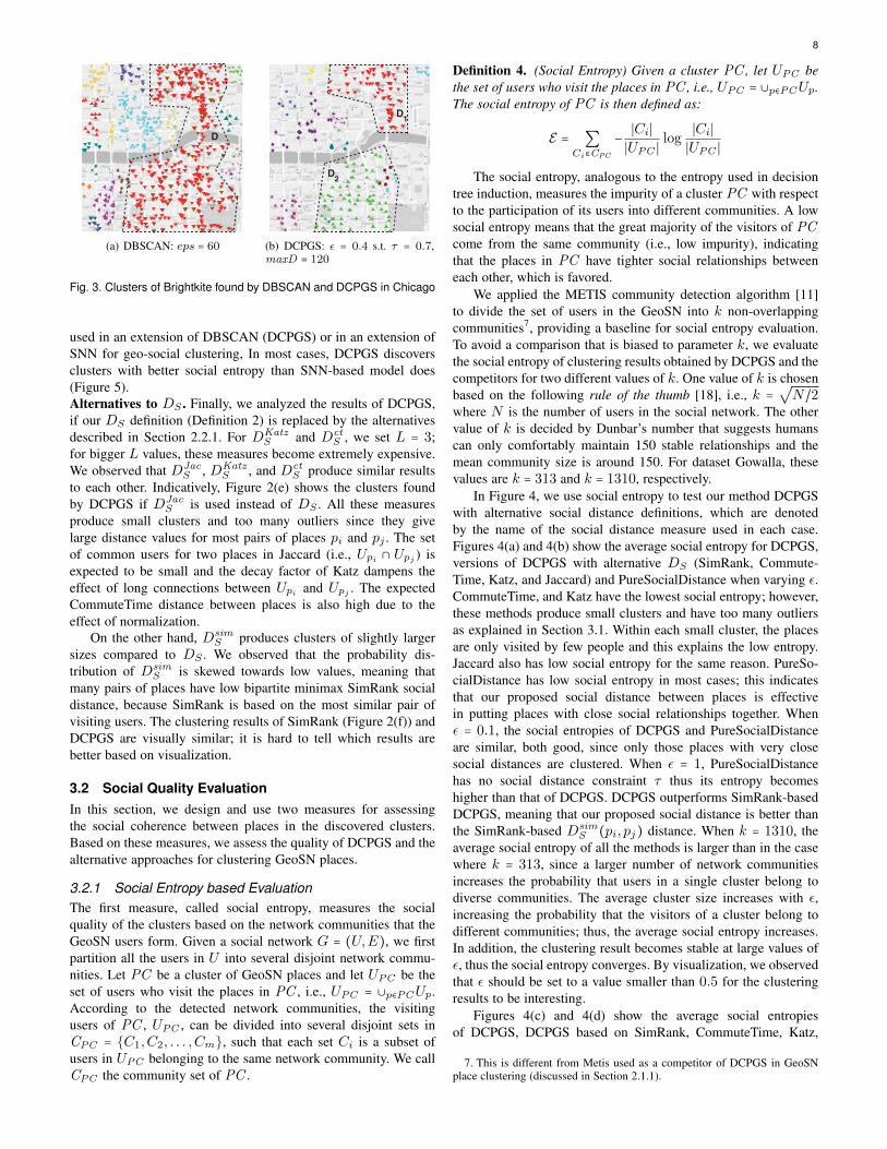
Geo-Social Splitting/Merging Criteria. Geo-social clusters thatare very close to each other are split correctly by DCPGS, whileDBSCAN may consider them as a single cluster due to theirspatial closeness; in other cases, clusters split by DBSCAN due torelatively low spatial density between them are merged by DCPGSbecause of their strong social ties. For example, consider regionA in Figures 2(a) and the corresponding region A′ in Figure 2(b),where DCPGS and DBSCAN detect clusters with totally differentlayouts. By tuning the parameters of DBSCAN, we are not ableto find the clusters found by DCPGS, because the densities ofthe two clusters in region A are similar and the two clusters areclose to each other. Thus, DBSCAN can only consider the placesin region A′ as either a single cluster or as several fragmentedclusters (Figure 2(b)), under different parameter settings. In certaincases, spatially dense clusters may be split by DCPGS because ofsome natural barriers, such as rivers, and walls. These barriersmake it inconvenient to travel from one side to the other, resultingin a splitting effect. As an example, in Figure 3, a cluster (regionD) found by DBSCAN is split into two DCPGS clusters (regionsD1 and D2) by the river, since the users on different river sidesare proved to have weak social connection. While it is possible forDBSCAN to find the two DCPGS clusters by reducing the value ofeps , its parameter settings in this case make some existing clustersdisappear, resulting in too many outliers.

Spatially Loose Clusters. Some geo-social clusters detected byDCPGS in region B of Figure 2(a) are considered as outliers byDBSCAN in the corresponding region B′ of Figure 2(b). RegionB′ is spatially too sparse to satisfy the density requirement ofDBSCAN, and thus most places inside it are filtered out as out-liers. However, the users who checked in those places have strongsocial relationships. Hence, geo-social clusters are discovered inregion B by DCPGS in Figure 2(a). While it is possible forDBSCAN to discover such spatially loose clusters by reducingthe density parameters, this would result in merging too manyclusters together, making denser clusters indistinguishable.

Fuzzy Boundary Clusters. Some DCPGS geo-social clustershave fuzzy boundaries with each other, which is reasonable inthe real world, since groups of socially connected users mayspatially overlap. On the other hand, DBSCAN produces clusterswith strict boundaries. For instance, in Figure 2(a), there is nostrict boundary between the two clusters enclosed in region C.Although PureSocialDistance, which is the other extreme method,also produces clusters with fuzzy boundaries (see Figure 2(c)), theclusters are spatially indistinguishable and they are not interesting,i.e., for the applications mentioned in the Introduction.Alternatives to DCPGS. We visually analyzed the results ofthe alternatives to DCPGS, i.e., SNN-based clustering modeland graph-based clustering models (LinkClustering and Metis),described in Section 2.1.1. LinkClustering and Metis producesimilar results; indicatively, we show the clusters produced byLinkClustering in Figure 2(d). LinkClustering produces thousandsof small clusters (average size around 3), which are typically notwell-separated spatially. Due to the sparsity of geo-social networkdata, the constructed place network contains many connectedcomponents that are disconnected with each other (e.g., the place

7

B

A

C

(a) DCPGS: ε = 0.4, τ = 0.7,maxD = 100

A′

B′

(b) DBSCAN: eps = 40 (c) PureSocialDistance: ε = 0.2, τ =1, maxD = 1000

(d) LinkClustering: τ = 0.7,maxD = 100

A

C

B

(e) Jaccard: ε = 0.4, τ = 0.7,maxD = 100

A

C

B

(f) SimRank: ε = 0.3, τ = 0.7,maxD = 100

40.72

40.73

40.74

40.75

−74.01 −74.00 −73.99 −73.98 −73.97

lon

lat

(g) SNN: epssnn = 1, maxD = 60

40.72

40.73

40.74

40.75

−74.01 −74.00 −73.99 −73.98 −73.97

lon

lat

d$names 0

1

2

3

4

5

10

20

30

40

50

d$cluster

(h) SNN: epssnn = 2, maxD = 60

40.72

40.73

40.74

40.75

−74.01 −74.00 −73.99 −73.98 −73.97

lon

lat

d$names 0

1

2

3

4

5

10

20

30

40

d$cluster

(i) SNN: epssnn = 3, maxD = 60

40.72

40.73

40.74

40.75

−74.01 −74.00 −73.99 −73.98 −73.97

lon

lat

d$names 0

1

2

3

4

5

2.5

5.0

7.5

10.0

d$cluster

(j) SNN: epssnn = 1, maxD = 120

40.72

40.73

40.74

40.75

−74.01 −74.00 −73.99 −73.98 −73.97

lon

lat

d$names 0

1

2

3

4

5

5

10

15

20

d$cluster

(k) SNN: epssnn = 3, maxD = 120

40.72

40.73

40.74

40.75

−74.01 −74.00 −73.99 −73.98 −73.97

lon

lat

10

20

30d$cluster

d$names 0

1

2

3

4

5

(l) SNN: epssnn = 5, maxD = 120

Fig. 2. Place clusters of Gowalla found in Manhattan

network built when τ = 0.7, maxD = 100, and ω = 0.5 contains34,496 connected components with 4.3 nodes and 8.2 edges onaverage). The clusters found by Metis are fewer and larger, butalso spatially indistinguishable. Metis ignores outliers; as a result,places belong to the same cluster may have low spatial proximityand social similarity.

Figures 2(g)–2(l) show the clusters found by the SNN-basedclustering model. Since DCPGS and SNN-based model only differin the way of measuring the closeness/similarity between places,by carefully tuning the parameters of SNN-based model, we try

to figure out whether it can discover similar clusters to those ofDCPGS. We observe that when maxD = 60 and epssnn = 1(Figure 2(g)), the SNN-based model indeed finds similar clustersin the areas highlighted by rectangles. As epssnn increases (Fig-ures 2(h) and 2(i)), the sizes of clusters decrease. This is becauselarge epssnn puts strict constraints on the places to be a memberof a cluster. When maxD = 120 and epssnn = 1 (Figure 2(j)),a big cluster is discovered by the SNN-based model. As epssnnincreases (Figures 2(k) and 2(l)), several clusters are identifiedfrom this big cluster. Although our geo-social distance can also be

8

!

(a) DBSCAN: eps = 60

D2

D1

(b) DCPGS: ε = 0.4 s.t. τ = 0.7,maxD = 120

Fig. 3. Clusters of Brightkite found by DBSCAN and DCPGS in Chicago

used in an extension of DBSCAN (DCPGS) or in an extension ofSNN for geo-social clustering, In most cases, DCPGS discoversclusters with better social entropy than SNN-based model does(Figure 5).Alternatives to DS . Finally, we analyzed the results of DCPGS,if our DS definition (Definition 2) is replaced by the alternativesdescribed in Section 2.2.1. For DKatz

S and DctS , we set L = 3;

for bigger L values, these measures become extremely expensive.We observed that DJac

S , DKatzS , and Dct

S produce similar resultsto each other. Indicatively, Figure 2(e) shows the clusters foundby DCPGS if DJac

S is used instead of DS . All these measuresproduce small clusters and too many outliers since they givelarge distance values for most pairs of places pi and pj . The setof common users for two places in Jaccard (i.e., Upi ∩ Upj ) isexpected to be small and the decay factor of Katz dampens theeffect of long connections between Upi and Upj . The expectedCommuteTime distance between places is also high due to theeffect of normalization.

On the other hand, DsimS produces clusters of slightly larger

sizes compared to DS . We observed that the probability dis-tribution of Dsim

S is skewed towards low values, meaning thatmany pairs of places have low bipartite minimax SimRank socialdistance, because SimRank is based on the most similar pair ofvisiting users. The clustering results of SimRank (Figure 2(f)) andDCPGS are visually similar; it is hard to tell which results arebetter based on visualization.

3.2 Social Quality EvaluationIn this section, we design and use two measures for assessingthe social coherence between places in the discovered clusters.Based on these measures, we assess the quality of DCPGS and thealternative approaches for clustering GeoSN places.

3.2.1 Social Entropy based EvaluationThe first measure, called social entropy, measures the socialquality of the clusters based on the network communities that theGeoSN users form. Given a social network G = (U,E), we firstpartition all the users in U into several disjoint network commu-nities. Let PC be a cluster of GeoSN places and let UPC be theset of users who visit the places in PC , i.e., UPC = ∪p∈PCUp.According to the detected network communities, the visitingusers of PC , UPC , can be divided into several disjoint sets inCPC = C1,C2, . . . ,Cm, such that each set Ci is a subset ofusers in UPC belonging to the same network community. We callCPC the community set of PC .

Definition 4. (Social Entropy) Given a cluster PC , let UPC bethe set of users who visit the places in PC , i.e., UPC = ∪p∈PCUp.The social entropy of PC is then defined as:

E = ∑Ci∈CPC

−∣Ci∣

∣UPC ∣log

∣Ci∣

∣UPC ∣

The social entropy, analogous to the entropy used in decisiontree induction, measures the impurity of a cluster PC with respectto the participation of its users into different communities. A lowsocial entropy means that the great majority of the visitors of PCcome from the same community (i.e., low impurity), indicatingthat the places in PC have tighter social relationships betweeneach other, which is favored.

We applied the METIS community detection algorithm [11]to divide the set of users in the GeoSN into k non-overlappingcommunities7, providing a baseline for social entropy evaluation.To avoid a comparison that is biased to parameter k, we evaluatethe social entropy of clustering results obtained by DCPGS and thecompetitors for two different values of k. One value of k is chosenbased on the following rule of the thumb [18], i.e., k =

√N/2

where N is the number of users in the social network. The othervalue of k is decided by Dunbar’s number that suggests humanscan only comfortably maintain 150 stable relationships and themean community size is around 150. For dataset Gowalla, thesevalues are k = 313 and k = 1310, respectively.

In Figure 4, we use social entropy to test our method DCPGSwith alternative social distance definitions, which are denotedby the name of the social distance measure used in each case.Figures 4(a) and 4(b) show the average social entropy for DCPGS,versions of DCPGS with alternative DS (SimRank, Commute-Time, Katz, and Jaccard) and PureSocialDistance when varying ε.CommuteTime, and Katz have the lowest social entropy; however,these methods produce small clusters and have too many outliersas explained in Section 3.1. Within each small cluster, the placesare only visited by few people and this explains the low entropy.Jaccard also has low social entropy for the same reason. PureSo-cialDistance has low social entropy in most cases; this indicatesthat our proposed social distance between places is effectivein putting places with close social relationships together. Whenε = 0.1, the social entropies of DCPGS and PureSocialDistanceare similar, both good, since only those places with very closesocial distances are clustered. When ε = 1, PureSocialDistancehas no social distance constraint τ thus its entropy becomeshigher than that of DCPGS. DCPGS outperforms SimRank-basedDCPGS, meaning that our proposed social distance is better thanthe SimRank-based Dsim

S (pi, pj) distance. When k = 1310, theaverage social entropy of all the methods is larger than in the casewhere k = 313, since a larger number of network communitiesincreases the probability that users in a single cluster belong todiverse communities. The average cluster size increases with ε,increasing the probability that the visitors of a cluster belong todifferent communities; thus, the average social entropy increases.In addition, the clustering result becomes stable at large values ofε, thus the social entropy converges. By visualization, we observedthat ε should be set to a value smaller than 0.5 for the clusteringresults to be interesting.

Figures 4(c) and 4(d) show the average social entropiesof DCPGS, DCPGS based on SimRank, CommuteTime, Katz,

7. This is different from Metis used as a competitor of DCPGS in GeoSNplace clustering (discussed in Section 2.1.1).

9

and Jaccard, and the graph-based clustering methods Metis andLinkClustering, when varying the social distance constraint τ .Similar to the case when ε varies, the social entropy increasesand then stabilizes as τ increases, except for the entropy of Metis,which keeps increasing due to the network partitioning methodol-ogy of Metis with the increase of τ , the constructed place networkbecomes less connected, however, due to its partitioning nature,Metis puts disconnected places in the constructed place networkinto same cluster. When τ is less than 0.5, the social entropyof CommuteTime is zero, since with these distance measures theplaces in each cluster are visited by only one person when τ < 0.5.Jaccard has low social entropy also due to the small sizes of itsclusters. For τ ≤ 0.1 SimRank-based DCPGS fails to find anyclusters, therefore the entropy is 0. After investigation, we foundthat there is no pair of places pi, pj with Dsim

S (pi, pj) < 0.2because of the decay factor φ. When τ = 0.2, SimRank has a lowsocial entropy, since only few (987) clusters of small size are foundcompared to the 3605 clusters discovered by DCPGS. After thepoint where the two approaches find a similar number of clusters(e.g., at τ = 0.5, SimRank finds 5880 clusters, while DCPGSfinds 6742 clusters), DCPGS has constantly lower entropy thanSimRank. In addition, DCPGS is less sensitive to τ compared toSimRank. DCPGS outperforms the two graph-based competitorsMetis and LinkClustering. As we observed by visualization, inpractice τ should be set to a value higher than 0.5, because avery tight social distance constraint creates too few and too smallgeo-social clusters.

Figures 4(e) and 4(f) show the average social entropies of thevarious versions of DCPGS and all the competitor approacheswhen varying the spatial distance constraint maxD (eps forDBSCAN). DCPGS is superior to SimRank-based DCPGS, DB-SCAN, LinkClustering and Metis for all values of maxD (eps).In general, the social entropies of all methods are not very sensitiveto maxD . For Gowalla, a good value for maxD is around 100;large maxD values result in clusters that are spatially too loose.

Figure 5 compares the social entropy of SNN-based model(when varying epssnn ) and DCPGS (when varying ε), whereSNN−60 and SNN−120 denote SNN-based model withmaxD = 60 and maxD = 120, respectively. Parameter τ is fixedat 0.7 and MinPts is set to 5. The first row of the x-axis representsthe values of ε in DCPGS, while the second row contains thevalues of epssnn in SNN-based model. The range of ε in DCPGSis [0,1]. Parameter epssnn in SNN is an integer in the range of[0,+∞). Small ε in DCPGS can be translated into large epssnnin SNN-based model, which indicates that the condition of a placebeing a core is that there should be enough places with small geo-social distances surrounding it. We observe that the social entropyof SNN-based model does not change much with epssnn and itis worse than DCPGS with small ε, and comparable with DCPGSwith large ε.

3.2.2 Community Score based EvaluationGiven a GeoSN place cluster PC , let UPC be the set of userswho visit the places in PC , i.e., UPC = ∪p∈PCUp. Assume eachUPC is a community in the GeoSN. We adopt the eight networkcommunity multi-criterion scores surveyed in [19] to computethe community score of UPC for each cluster PC . Figure 6compares the results of DCPGS and its alternatives on Gowalla(Katz is omitted because its result is quite similar to that ofCommuteTime), in terms of the internal density and conductancescores. We group the clusters discovered by each method by size

DCPGS DBSCAN PureSocialDistance Jaccard × SimRank ◻ Katz CommuteTime ∎ LinkClustering ▷ Metis

0.1 0.2 0.3 0.4 0.5 0.6 0.7 0.8 0.9 10

0.5

1

1.5

2

2.5

ε

Soc

ial E

ntro

py

(a) k = 3130.1 0.2 0.3 0.4 0.5 0.6 0.7 0.8 0.9 10

0.5

1

1.5

2

2.5

ε

Soc

ial E

ntro

py

(b) k = 1310

0 0.1 0.2 0.3 0.4 0.5 0.6 0.7 0.8 0.9 10

0.5

1

1.5

2

2.5

3

3.5

4

τ

Soc

ial E

ntro

py

(c) k = 3130 0.1 0.2 0.3 0.4 0.5 0.6 0.7 0.8 0.9 1

0

0.5

1

1.5

2

2.5

3

3.5

4

τ

Soc

ial E

ntro

py

(d) k = 1310

10 50 100 150 200 250 3000

0.5

1

1.5

2

2.5

3

3.5

(DBSCAN) or (others)

Soc

ial E

ntro

py

meps maxD

(e) k = 313

10 50 100 150 200 250 3000

0.51

1.52

2.53

3.54

(DBSCAN) or (others)

Soc

ial E

ntro

py

mmaxDeps

(f) k = 1310

Fig. 4. Social entropy evaluation in Gowalla

0.110

0.29

0.38

0.47

0.56

0.65

0.74

0.83

0.92

1.01

ε (epssnn)

0.0

0.5

1.0

1.5

2.0

2.5

Soci

al E

ntro

py

DCPGSSNN-60SNN-120

(a) k = 313

0.110

0.29

0.38

0.47

0.56

0.65

0.74

0.83

0.92

1.01

ε (epssnn)

0.0

0.5

1.0

1.5

2.0

2.5

Soci

al E

ntro

py

DCPGSSNN-60SNN-120

(b) k = 1310

Fig. 5. Social entropy of SNN geo-social clusters in Gowalla

and compute and plot the average community score (i.e., internaldensity and conductance) for each cluster size group. The resultsbased on the other six criteria of [19] are similar and we omitthem due to lack of space. The internal density of UPC is definedby 1−mUPC

/(∣UPC ∣(∣UPC ∣− 1)/2), where mUPCis the number

of edges, which belongs to E and whose two endpoints are bothin UPC , mUPC

= ∣(u, v)∣u ∈ UPC , v ∈ UPC , (u, v) ∈ E∣. Con-ductance is the fraction of edges, which belongs to E, from nodesof UPC that point outside UPC , i.e., oUPC

/(2mUPC+ oUPC

),where oUPC

= ∣(u, v)∣u ∈ UPC , v ∉ UPC , (u, v) ∈ E∣. Letf(UPC ) be the community score of PC , based on either internal

10

density or conductance; a smaller value of f(UPC ) indicatesbetter social quality.

0 50 100 150 200 250 300 350 4000.55

0.6

0.65

0.7

0.75

0.8

0.85

0.9

0.95

1

Cluster size

Inte

rnal

den

sity

PureSocialDistanceDBSCANSimRankDCPGS

(a) Internal Density

0 50 100 150 200 250 300 350 4000.75

0.8

0.85

0.9

0.95

1

Cluster sizeCo

nduc

tanc

e

PureSocialDistanceDBSCANSimRankDCPGS

(b) Conductance

0 50 100 150 200 250 300 350 4000.55

0.6

0.65

0.7

0.75

0.8

0.85

0.9

0.95

1

Inte

rnal

den

sity

Cluster size

MetisLinkClusteringCommuteTimeJaccardDCPGS

(c) Internal Density

0 50 100 150 200 250 300 350 4000.75

0.8

0.85

0.9

0.95

1

Con

duct

ance

Cluster size

MetisLinkClusteringCommuteTimeJaccardDCPGS

(d) Conductance

Fig. 6. Community score evaluation in Gowalla

As Figures 6(a) and 6(c) show, the internal density increaseswith the cluster size. As the size of a place cluster increases, thedenominator of the internal density formula increases quadrati-cally while the number of social links between users in the cluster(i.e., the numerator) does not increase at the same pace. On theother hand, Figures 6(b) and 6(d) show that conductance initiallydecreases as the size of a cluster increases and fluctuates randomlyfor larger UPC sizes, which is in line with the observations in [19].In Figure 6, we observe that the geo-social clusters discoveredby DCPGS have better community scores (i.e., lower internaldensity and conductance scores) compared to all competitors,except PureSocialDistance. Since PureSocialDistance uses oursocial distance in clustering and disregards spatial proximity, itssocial quality is expected to be better than that of DCPGS; still, asshown in Figure 2(c), its clusters are not distinguishable spatially.DCPGS outperforms DBSCAN and SimRank-based DCPGS. Thequality gap between DCPGS and the 3 competitors in Figure 6(a)and 6(b) narrows as the size of clusters increases, since it is moredifficult for a larger UPC (usually obtained from a larger PC )to maintain a community-like structure compared to a smallerUPC [19]. This indicates that our social distance is effective infinding geo-social clusters with small or medium size. DCPGSis also generally better than the four competitors in Figures 6(c)and 6(d). CommuteTime has better community scores when thecluster size is around 50. Most community scores of Jaccard,CommuteTime, LinkClustering, and Metis concentrate at the top-left corner of Figures 6(c) and 6(d), which indicates that thesecompetitors have limited ability to discover geo-social clustersof various sizes. Furthermore, the quality gap between DCPGSand the five competitors in Figures 6(c) and 6(d) grows when thecluster size increases. We conclude that DCPGS (paired with oursocial distance measure) is the most effective method in findinggeo-social clusters with both good social quality and identifiablespatial contour.

3.3 Temporal Effects on Geo-Social ClustersIn this section, we illustrate the discovered temporal-geo-socialclusters in the area of Manhattan on the Gowalla dataset and in thearea of Chicago on the Brightkite dataset using the three methodsintroduced in Section 2.3.History-Frame Geo-Social Clustering. Figure 7 shows thetemporal-geo-social clusters found using continuous historyframe method in periods 01/08/2009–31/01/2010, 01/02/2010–31/07/2010, and 01/08/2010-31/01/2011 in the area of Manhattan.We observe that some clusters evolve over time. For instance, thecluster in region A first expanded and then shrinked. During period01/02/2010–31/07/2010, there are multiple clusters in region B,while in period 01/08/2010-31/01/2011, those clusters are mergedinto one big cluster. In region C, before there exists no cluster,while later a new cluster appeared. Figure 8 shows the temporal-geo-social clusters found using the periodic history frames, i.e., onworking days and weekends. We observe different place clusterson working days and weekends which is expected, since normallypeople visit places related to work on working days, while visitentertainment places on weekends.

40.72

40.73

40.74

40.75

−74.01 −74.00 −73.99 −73.98 −73.97lon

lat

20

40

60

d$cluster

d$names 0

1

2

3

4

5

(a) Working Days

40.72

40.73

40.74

40.75

−74.01 −74.00 −73.99 −73.98 −73.97lon

lat

10

20

30

40

d$cluster

d$names 0

1

2

3

4

5

(b) Weekends

Fig. 8. Periodic History Frame Geo-Social Clustering in Manhattan: ε =0.5, MinPts = 5, maxD = 120, τ = 0.7, ω = 0.5.

Temporally Contributing Users. Figure 9 shows the temporal-geo-social clusters found in Manhattan when parameter θ oftemporally contributing users is set to 1 week, 1 month, and6 months, respectively. When θ is a short time interval (e.g., 1week), the result reveals that the places in the same clusters arerevisited by socially connected users within a short period of time.As θ increases, the temporal-social distances between more placesdecrease, thus as expected (1) some clusters expand, (2) multipleclusters merge (e.g., regions A and B), (3) new clusters are found(e.g., region C). For marketing and management purpose, peoplemay be interested in both the short term and long term clusters.Damping Window. In Figure 11, we show the temporal-geo-social clusters found by the damping window method in Man-hattan, where the starting time is 01/02/2009 and the currenttime is set to 31/07/2010 and 31/01/2011, respectively. To betterunderstand the effect of the damping window, Figure 10 shows theclusters found by DCPGS on the same data in the same periods asthe damping window method. We observe that both the size of theclusters and the number of clusters found by the damping windoware smaller than DCPGS. This is expected, since weighing the olddata less increases the temporal-social distances between places.Under the same parameter setting, more regions in the dampingwindow are considered as sparse. However, the advantage of thedamping window is offering the up-to-date clustering result. As we

11

40.72

40.73

40.74

40.75

−74.01 −74.00 −73.99 −73.98 −73.97lon

lat

d$names 0

1

2

3

4

5

5

10

15d$clusterA

(a) 01/08/2009–31/01/2010

40.72

40.73

40.74

40.75

−74.01 −74.00 −73.99 −73.98 −73.97lon

lat

d$names 0

1

2

3

4

5

20

40

60

d$clusterA

B

C

(b) 01/02/2010–31/07/2010

40.72

40.73

40.74

40.75

−74.01 −74.00 −73.99 −73.98 −73.97lon

lat

d$names 0

1

2

3

4

5

10

20

30

40

d$clusterA

B

C

(c) 01/08/2010-31/01/2011

Fig. 7. Continuous History Frame Geo-Social Clustering in Manhattan: ε = 0.5, MinPts = 5, maxD = 120, τ = 0.7, ω = 0.5.

40.72

40.73

40.74

40.75

−74.01 −74.00 −73.99 −73.98 −73.97lon

lat

d$names 0

1

2

3

4

5

10

20

30

40

50

d$cluster

AB

C

(a) θ = 1 week

40.72

40.73

40.74

40.75

−74.01 −74.00 −73.99 −73.98 −73.97lon

lat

d$names 0

1

2

3

4

5

20

40

60d$cluster

AB

C

(b) θ = 1 month

40.72

40.73

40.74

40.75

−74.01 −74.00 −73.99 −73.98 −73.97lon

lat

d$names 0

1

2

3

4

5

20

40

60

d$cluster

AB

(c) θ = 6 months

Fig. 9. Temporally Contributing Users in Manhattan: ε = 0.5, MinPts = 5, maxD = 120, τ = 0.7, ω = 0.5

can see in Figure 11, the discovered clusters for the two periods aredifferent, which are sensitive to time. For instance, by 31/07/2010,clusters are found on Lafayette St., while by 31/01/2011, clustersare found close to Washington Square Park. Nevertheless, it isnot easy to notice these interesting up-to-date small clusters inFigure 10 because of the accumulated old data.

In summary, the three ways of considering the temporalinformation in the geo-social clustering yield different temporal-geo-social clusters, which may serve various purposes of analysisand investigation. The history-frame method offers the evolutionof clusters over time. The damping window method generatesthe up-to-date clusters. The temporally contributing user methodshows the places that are revisited within a period of time. Moreresults from the area of Chicago on the Brightkite data set can befound in Appendix A.Social Entropy based Evaluation Figure 12 shows the socialentropy of the temporal-geo-social clusters discovered by thethree methods introduced in Section 2.3 compared with the socialentropy of the geo-social clusters found by DCPGS. Recall that alow social entropy means that the great majority of the visitors ofa place cluster come from the same community, indicating that theplaces in the cluster have tighter social relationships between eachother. We observe that the clusters found by the damping window

40.72

40.73

40.74

40.75

−74.01 −74.00 −73.99 −73.98 −73.97lon

lat

d$names 0

1

2

3

4

5

20

40

60d$cluster

(a) 01/02/2009–31/07/2010

40.72

40.73

40.74

40.75

−74.01 −74.00 −73.99 −73.98 −73.97lon

lat

d$names 0

1

2

3

4

5

20

40

60

d$cluster

(b) 01/02/2009-31/01/2011

Fig. 10. DCPGS in Manhattan: ε = 0.5, MinPts = 5, maxD = 120, τ =0.7, ω = 0.5

method (DCPGSDW-Exp) and the temporally contributing usermethod (DCPGSTT) have better (lower) social entropy, comparedto the result found by DCPGS that does not consider the tem-porally information. Furthermore, the improvement achieved bydamping window method is larger than that of the temporallycontributing user method. However, the social entropy of the

12

40.72

40.73

40.74

40.75

−74.01 −74.00 −73.99 −73.98 −73.97lon

lat

d$names 0

1

2

3

4

5

2.5

5.0

7.5

d$cluster

(a) 01/02/2009–31/07/2010

40.72

40.73

40.74

40.75

−74.01 −74.00 −73.99 −73.98 −73.97lon

lat

d$names 0

1

2

3

4

5

2.5

5.0

7.5

10.0d$cluster

(b) 01/02/2009-31/01/2011

Fig. 11. Damping Window in Manhattan: ε = 0.5, MinPts = 5, maxD =120, τ = 0.7, ω = 0.5

clusters found by the history frame method (DCPGSHF) is worsethan the result of DCPGS. DCPGSHF in fact splits the wholedata into several sub-datasets based on time frames and performsclustering on these sub-datasets. The social entropies of theclusters from these sub-datasets should not necessarily be smallerthan the clusters from the whole data. DCPGSTT and DCPGSDW-Exp require more intra temporal closeness among places withinthe temporal-geo-social cluster. The smaller entropies of thesetwo methods indicates that temporal constraints can enhance thesocial connections within a cluster. According to the analysisin previously sections, the result of the community score basedevaluation is consistent with the result of the social entropy basedevaluation, and thus is omitted.

4 RELATED WORK

Our clustering problem is related to various research topics,including traditional spatial clustering, using mobility data toanalyze places, clustering using spatial and non-spatial attributes,studying the relationship between spatial and social attributes,community detection, and other work on GeoSNs.Spatial Clustering. Spatial clustering algorithms, surveyed in[20], are divided into three categories: partitioning, hierarchicaland density-based clustering. Partitioning methods, including k-means, k-medoids, and CLARANS [21], are good at findingspherical-shaped clusters in small and medium-sized datasets.They need a pre-defined parameter k to specify the number ofclusters obtained. However, partitioning methods are not able todetect clusters of arbitrary shapes. Hierarchical clustering tech-niques, such as BIRCH [22], Chameleon [23] and CURE [24],assign objects to clusters in two fashions: agglomerative (bottom-up) and divisive (top-down). Hierarchical clustering methods donot have well-defined termination criteria and cannot correct theresult if some objects are assigned to the wrong clusters at anearly stage. Density-based clustering methods, like DBSCAN [1],[25], discover clusters of arbitrary shapes and sizes. Objects indense regions are grouped as clusters, while objects in sparseregions are labeled as outliers. OPTICS [26] is an extension ofDBSCAN, which generates an augmented ordering of the datasetthat captures its density-based clustering structure at differentgranularities. DENCLUE [27] models the overall point densityanalytically as the sum of influence functions of the data points.Clusters can then be identified by determining density-attractorsand clusters of arbitrary shapes can be easily described by a

0.1 0.2 0.3 0.4 0.5 0.6 0.7 0.8 0.9 1.0ε

0.0

0.5

1.0

1.5

2.0

2.5

Soci

al E

ntro

py

DCPGSDCPGSHF090801-100131DCPGSHF100201-100731DCPGSHF100801-110131

(a) k = 313

0.1 0.2 0.3 0.4 0.5 0.6 0.7 0.8 0.9 1.0ε

0.0

0.5

1.0

1.5

2.0

2.5

Soci

al E

ntro

py

DCPGSDCPGSHF090801-100131DCPGSHF100201-100731DCPGSHF100801-110131

(b) k = 1310

History-Frame Geo-Social Clustering

0.1 0.2 0.3 0.4 0.5 0.6 0.7 0.8 0.9 1.0ε

0.0

0.5

1.0

1.5

2.0

2.5

Soci

al E

ntro

py

DCPGSDCPGSDW-Exp-090201-100731DCPGSDW-Exp-090201-110131DCPGS-090201-100731

(c) k = 313

0.1 0.2 0.3 0.4 0.5 0.6 0.7 0.8 0.9 1.0ε

0.0

0.5

1.0

1.5

2.0

2.5

3.0

Soci

al E

ntro

py

DCPGSDCPGSDW-Exp-090201-100731DCPGSDW-Exp-090201-110131DCPGS-090201-100731

(d) k = 1310

Damping Window

0.1 0.2 0.3 0.4 0.5 0.6 0.7 0.8 0.9 1.0ε

0.0

0.5

1.0

1.5

2.0

2.5

Soci

al E

ntro

py

DCPGSDCPGSTT-1WDCPGSTT-1MDCPGSTT-6M

(e) k = 313

0.1 0.2 0.3 0.4 0.5 0.6 0.7 0.8 0.9 1.0ε

0.0

0.5

1.0

1.5

2.0

2.5

3.0

Soci

al E

ntro

py

DCPGSDCPGSTT-1WDCPGSTT-1MDCPGSTT-6M

(f) k = 1310

Temporally Contributing Users

Fig. 12. Social entropy of temporal-geo-social clusters in Gowalla

simple equation based on the overall density function. Later, anadaptive method [28] that automatically determines the parameterε of DBSCAN is proposed. GDBSCAN [29] is a generalizationof DBSCAN that clusters point objects as well as spatiallyextended objects according to both their spatial and their non-spatial attributes. A-DBSCAN [30] is an anytime density-basedclustering algorithm which is applicable to many complex datasuch as trajectory and medical data. It uses a sequence of lowerbounding functions of the true distance function to producemultiple approximate results of the true density-based clusters.Recently, Gan and Tao [31] discussed hardness of DBSCAN andproposed an efficient approximate version. Our work adopts thedensity-based clustering framework to find place clusters in a geo-social network, by considering both the spatial distance and thesocial coherence of the places.Analysis of Places based on Mobility Data. Brilhante et al. [10]detect “communities” of places of interest (POIs) on a map basedon how strongly the places are correlated in sequences of visitsby mobile users. Different from our work, the social relationshipsbetween the users who visit the places and the spatial distancesbetween places are disregarded. The co-existence of places in thevisiting histories of users is the only criterion used for clustering.The proposed solution generates a graph G that connects pairsPOIs according to the nature of their co-existence in sequencesof user visits and then employs a classic algorithm for community

13

detection on G to identify the place communities. Andrienko et al.[32] present an analysis and visualization tool, which first identi-fies interesting events of moving objects (e.g., instances of slowcar movements), then spatially clusters these events, using density-based clustering to derive a set of significant places (e.g., regionswhere traffic jams occur), and finally applies visual analytics toaggregate and analyze the events with respect to parameters suchas location, time and direction of movement. Noulas et al. [33]perform an empirical analysis of the topological properties ofplace networks formed by the trajectories of mobile users. Theynote their resemblance to online social networks in terms of heavy-tailed degree distributions, triadic closure mechanisms and thesmall world property.

Clustering based on Spatial and Non-Spatial Attributes. Clus-tering objects based on spatial and non-spatial attributes findsapplications in different areas, such as computer vision, GIS, andsocial networks. Yu et al. [34] cluster pixels considering both theRGB color vectors and spatial proximity that is useful in naturalimage segmentation. Gennip et al. [35] use spectral clustering toidentify communities in a graph where nodes are gang membersand weighted edges indicate the gang members’ social interactionsand geographic locations. Zhang et al. [36] apply clustering byadjusting the spatial distance between two objects according to thenon-spatial attribute values between them. EBSCAN [37] clustersgeoreferenced big data based on not only spatial information butalso human behavior derived from geographical features.

Spatial-Social Relationship. The relationship between geographyand social structure has been long studied by sociologists. Re-searchers have found that the likelihood of friendship with a per-son is decreasing with distance, which has been observed withincolleges [38], new housing developments [39], and projects forthe elderly [40]. Scellato et al. [4] performed a quantitative studyon the socio-spatial properties of users in GeoSNs. By utilizingsocial and spatial properties of GeoSNs, the same research groupproposed a link prediction model [5]. Backstrom et al. [41] predictthe location of an individual from a sparse set of known userlocations using the relationship between geography and friendship.Wang et al. [15] find that the similarity between the movementsof two individuals strongly correlates with their proximity in thesocial network. This correlation is used as a tool for link predictionin a social network. Pham et al. [42] propose an entropy-basedmodel (EBM) that not only infers social connections but alsoestimates the strength of social connections by analyzing people’sco-occurrences in space and time. Different from existing work,we neither study the spatial-social relationship nor do prediction orrecommendation utilizing this relationship. We perform density-based clustering of GeoSN places considering both the spatialdistances between them and the social relationships between usersthat visit the places.

Detecting and Evaluating Communities in Networks. Thereare many existing works on network community detection andclustering of nodes in a graph using only the network distancebetween nodes [43], [44], [45], [46]. SCAN [45] is an algorithmthat detects clusters, hubs, and outliers in networks. [46] proposedpartitioning, hierarchical and density-based algorithms to clusterobjects on spatial networks, based on shortest-path distance. [19]summarized and empirically evaluated algorithms for networkcommunity detection. In Section 3.2.2, we have used networkcommunity quality measures [19] to evaluate the social qualityof the place clusters found by our algorithms.

Importing Time into Clustering. Previous works on spatio-temporal data clustering typically include the time concept in thedata or algorithms as a threshold or as a parameter of the distancefunction. Some works transform the spatio-temporal clusteringproblem to a multi-sequence spatial data clustering problem [47].The history-frame clustering method that we propose is simi-lar to multi-sequence clustering. Trasarti [48] imported time todata as a new dimension. Thus clustering is performed on highdimensional data using standard distance measure such as theEuclidean distance. In this method, the time effect may be re-duced compared with many other dimensions. ST-DBSCAN [49]improves DBSCAN to cluster spatialtemporal data where a timeperiod attached to the spatial data expresses when it was validor stored in the database. During clustering, spatio-temporal dataare filtered by retaining only the temporal neighbors and theircorresponding spatial values. Two objects are temporal neighborsif the values of these objects are observed in consecutive time unitssuch as consecutive days in the same year or in the same day inconsecutive years. Similarly, [50], [51], [52] integrate the temporalinformation into the distance function used for clustering. In otherwords, two objects have to be close in terms of time (e.g., timedifference lower than 1 hour) in order to belong to the same cluster.Different from existing works that simply set a time threshold anduse it as an additional filtering step when computing distancesbetween objects, the damping window and temporally contributinguser methods in the paper take the temporal information and theusers’ social relationships into account simultaneously.

5 CONCLUSION

In this paper, we studied for the first time the problem of Density-based Clustering Places in Geo-Social Networks (DCPGS). Ourclustering model extends the density-based clustering paradigm toconsider both the spatial and social distances between places. Wedefined a new measure for the social distance between places,considering the social ties between users that visit them. Ourmeasure is shown to be more effective to compute, comparedto more complex ones based on node-to-node graph proximityand SNN-based model. We analyzed the effectiveness of DCPGSvia case studies and demonstrated that DCPGS can discoverclusters with interesting properties (i.e., barrier-based splitting,spatially loose clusters, clusters with fuzzy boundaries), whichcannot be found by merely using spatial clustering. To improvethe quality of clusters, we incorporate the temporal informationof the checkins using three different ways that satisfy differentanalysis and investigation requirements. Besides, we designed twoevaluation measures to quantitatively evaluate the social quality ofclusters detected by DCPGS or competitors, called social entropyand community score, which also confirm that DCPGS is moreeffective than alternative approaches and the temporal dimensionfurther improves the quality of the clusters.

ACKNOWLEDGMENT

This work was supported in part by NSFC grant No. 61502310 andby the European Unions Horizon 2020 research and innovationprogramme under grant agreement No 657347.

REFERENCES

[1] M. Ester, H.-P. Kriegel, J. Sander, and X. Xu, “A density-based algorithmfor discovering clusters in large spatial databases with noise,” in KDD,1996.

14

[2] P.-N. Tan, M. Steinbach, and V. Kumar, Introduction to Data Mining.Addison-Wesley, 2005.

[3] J. Shi, N. Mamoulis, D. Wu, and D. W. Cheung, “Density-based placeclustering in geo-social networks,” in SIGMOD, 2014, pp. 99–110.

[4] S. Scellato, A. Noulas, R. Lambiotte, and C. Mascolo, “Socio-spatialproperties of online location-based social networks,” in ICWSM, 2011.

[5] S. Scellato, A. Noulas, and C. Mascolo, “Exploiting place features in linkprediction on location-based social networks,” in KDD, 2011.

[6] D.-N. Yang, C.-Y. Shen, W.-C. Lee, and M.-S. Chen, “On socio-spatialgroup query for location-based social networks,” in KDD, 2012.

[7] N. Armenatzoglou, S. Papadopoulos, and D. Papadias, “A general frame-work for geo-social query processing,” PVLDB, vol. 6, no. 10, pp. 913–924, 2013.

[8] L. Ertoz, M. Steinbach, and V. Kumar, “Finding clusters of differentsizes, shapes, and densities in noisy, high dimensional data,” in SDM,2003, pp. 47–58.

[9] Y.-Y. Ahn, J. P. Bagrow, and S. Lehmann, “Link communities revealmultiscale complexity in networks,” Nature, vol. 466, pp. 761–764, 2010.

[10] I. R. Brilhante, M. Berlingerio, R. Trasarti, C. Renso, J. A. F. de Macedo,and M. A. Casanova, “Cometogether: Discovering communities of placesin mobility data,” in MDM, 2012.

[11] G. Karypis and V. Kumar, “A fast and high quality multilevel schemefor partitioning irregular graphs,” SIAM Journal on scientific Computing,vol. 20, no. 1, pp. 359–392, 1998.

[12] S. Milgram, “The small world problem,” Psychology today, vol. 2, no. 1,pp. 60–67, 1967.

[13] J. Leskovec, J. M. Kleinberg, and C. Faloutsos, “Graph evolution:Densification and shrinking diameters,” TKDD, vol. 1, no. 1, 2007.

[14] G. Jeh and J. Widom, “Simrank: A measure of structural-context simi-larity,” Stanford InfoLab, Technical Report, 2001.

[15] D. Wang, D. Pedreschi, C. Song, F. Giannotti, and A.-L. Barabasi,“Human mobility, social ties, and link prediction,” in KDD, 2011.

[16] C. Wang, V. Satuluri, and S. Parthasarathy, “Local probabilistic modelsfor link prediction,” in ICDM, 2007.

[17] P. Sarkar and A. W. Moore, “A tractable approach to finding closesttruncated-commute-time neighbors in large graphs,” in UAI, 2007.

[18] K. V. Mardia, J. Kent, and J. Bibby, Multivariate analysis (probabilityand mathematical statistics). Academic Press London, 1980.

[19] J. Leskovec, K. J. Lang, and M. W. Mahoney, “Empirical comparison ofalgorithms for network community detection,” in WWW, 2010.

[20] J. Han and M. Kamber, Data Mining: Concepts and Techniques. MorganKaufmann, 2000.

[21] R. T. Ng and J. Han, “Efficient and effective clustering methods forspatial data mining,” in VLDB, 1994.

[22] T. Zhang, R. Ramakrishnan, and M. Livny, “Birch: An efficient dataclustering method for very large databases,” in SIGMOD, 1996.

[23] G. Karypis, E.-H. Han, and V. Kumar, “Chameleon: Hierarchical cluster-ing using dynamic modeling,” IEEE Computer, vol. 32, no. 8, pp. 68–75,1999.

[24] S. Guha, R. Rastogi, and K. Shim, “Cure: An efficient clusteringalgorithm for large databases,” in SIGMOD, 1998.

[25] A. Gunawan, “A faster algorithm for dbscan,” Master Thesis, TechnischeUniversity Eindhoven, March 2013.

[26] M. Ankerst, M. M. Breunig, H.-P. Kriegel, and J. Sander, “Optics:Ordering points to identify the clustering structure,” in SIGMOD, 1999.

[27] A. Hinneburg and D. A. Keim, “An efficient approach to clustering inlarge multimedia databases with noise,” in KDD, 1998.

[28] S. Jahirabadkar and P. Kulkarni, “Short communication: Algorithm todetermine epsilon-distance parameter in density based clustering,” ExpertSyst. Appl., vol. 41, no. 6, pp. 2939–2946, 2014.

[29] J. Sander, M. Ester, H.-P. Kriegel, and X. Xu, “Density-based clusteringin spatial databases: The algorithm gdbscan and its applications,” DataMin. Knowl. Discov., vol. 2, no. 2, pp. 169–194, 1998.

[30] S. T. Mai, X. He, J. Feng, C. Plant, and C. Bohm, “Anytime density-based clustering of complex data,” Knowl. Inf. Syst., vol. 45, no. 2, pp.319–355, 2015.

[31] J. Gan and Y. Tao, “Dbscan revisited: Mis-claim, un-fixability, andapproximation,” in SIGMOD, 2015, pp. 519–530.

[32] G. L. Andrienko, N. V. Andrienko, C. Hurter, S. Rinzivillo, and S. Wro-bel, “Scalable analysis of movement data for extracting and exploringsignificant places,” IEEE TVCG, vol. 19, no. 7, pp. 1078–1094, 2013.

[33] A. Noulas, B. Shaw, R. Lambiotte, and C. Mascolo, “Topological prop-erties and temporal dynamics of place networks in urban environments,”in WWW, 2015, pp. 431–441.

[34] Z. Yu, O. C. Au, R. Zou, W. Yu, and J. Tian, “An adaptive unsupervisedapproach toward pixel clustering and color image segmentation,” PatternRecognition, vol. 43, no. 5, pp. 1889–1906, 2010.

[35] Y. van Gennip, B. Hunter, R. Ahn, P. Elliott, K. Luh, M. Halvorson,S. Reid, M. Valasik, J. Wo, G. E. Tita, A. L. Bertozzi, and P. J.Brantingham, “Community detection using spectral clustering on sparsegeosocial data,” CoRR, vol. abs/1206.4969, 2012.

[36] B. Zhang, W. J. Yin, M. Xie, and J. Dong, “Geo-spatial clusteringwith non-spatial attributes and geographic non-overlapping constraint:A penalized spatial distance measure,” in PAKDD, 2007.

[37] S. Yokoyama, A. Bogardi-Meszoly, and H. Ishikawa, “Ebscan: Anentanglement-based algorithm for discovering dense regions in large geo-social data streams with noise,” in LBSN, 2015, pp. 7:1–7:10.

[38] J. Q. Stewart, “An inverse distance variation for certain social influence,”Science, vol. 93, no. 2404, pp. 89–90, 1941.

[39] L. Festinger, S. Schachter, and K. Back, “Social pressures in informalgroups: a study of human factors in housing,” Stanford Univ. Pr., 1963.

[40] L. Nahemow and M. Lawton, “Similarity and propinquity in friendshipformation,” Journal of Personality and Social Psychology, vol. 32, no. 2,pp. 205–213, 1975.

[41] L. Backstrom, E. Sun, and C. Marlow, “Find me if you can: Improvinggeographical prediction with social and spatial proximity,” in WWW,2010.

[42] H. Pham, C. Shahabi, and Y. Liu, “Ebm: an entropy-based model to infersocial strength from spatiotemporal data,” in SIGMOD, 2013.

[43] C. Tantipathananandh, T. Y. Berger-Wolf, and D. Kempe, “A frameworkfor community identification in dynamic social networks,” in KDD, 2007.

[44] A. Clauset, M. E. Newman, and C. Moore, “Finding community structurein very large networks,” Physical review E, vol. 70, no. 6, 2004.

[45] X. Xu, N. Yuruk, Z. Feng, and T. A. J. Schweiger, “Scan: a structuralclustering algorithm for networks,” in KDD, 2007.

[46] M. L. Yiu and N. Mamoulis, “Clustering objects on a spatial network,”in SIGMOD, 2004.

[47] H. F. Tork, “Spatio-temporal clustering methods classification,” in DSIE,2012.

[48] R. Trasarti, “Mastering the spatio-temporal knowledge discovery pro-cess,” Ph.D. dissertation, Department of Computer Science, Universityof Pisa, 2010.

[49] D. Birant and A. Kut, “St-dbscan: An algorithm for clustering spatial-temporal data,” Data Knowl. Eng., vol. 60, no. 1, pp. 208–221, 2007.

[50] M. Wang, A. Wang, and A. Li, “Mining spatial-temporal clusters fromgeo-databases,” in ADMA, 2006, pp. 263–270.

[51] G. Andrienko and N. Andrienko, “Interactive cluster analysis of diversetypes of spatiotemporal data,” SIGKDD Explor. Newsl., vol. 11, no. 2,pp. 19–28, 2010.

[52] D. Fitrianah, A. N. Hidayanto, H. Fahmi1, J. L. Gaol, and A. M.Arymurthy, “St-agrid: A spatio temporal grid density based clusteringand its application for determining the potential fishing zones,” IJSEIA,vol. 9, no. 1, 2015.

Dingming Wu is an assistant professor with Col-lege of Computer Science & Software Engineer-ing, Shenzhen University, China. She receivedthe Ph.D. degree in Computer Science in 2011from Aalborg University, Denmark. Her generalresearch area is data management and mining,including data modeling, database design, andquery languages, efficient query and update pro-cessing, indexing, and mining algorithms.

Jieming Shi received his bachelors degreeof science from the department of ComputerScience and Technology in Nanjing University,2011, and his PhD in computer science fromthe University of Hong Kong. He is now a staffresearcher at Lenovo big data lab in Hong Kong.His research interests include geo-social net-work mining, knowledge graph management,and query processing on spatial-textual data.

Nikos Mamoulis received the diploma in com-puter engineering and informatics in 1995 fromthe University of Patras, Greece, and the PhDdegree in computer science in 2000 fromHKUST. He is currently a faculty member at theDepartment of Computer Science and Engineer-ing, University of Ioannina. His research focuseson the management and mining of complex datatypes, privacy and security in databases, anduncertain data management.

15

APPENDIX ATEMPORAL-GEO-SOCIAL CLUSTER EVALUATION

History-Frame Geo-Social Clustering. Figures 17 show theplace clusters found using continuous history frame methodin periods 01/03/2008–31/08/2008, 01/09/2008–28/02/2009, and01/03/2009-31/08/2009 in Chicago. Similar to the result of Man-hattan, clusters change with time. Take region A as an example.The cluster first shrinks and then becomes multiple clusters.Figure 13 shows the temporal-geo-social clusters found using theperiodic history frames, i.e., on working days and weekends. Asexpected, different place clusters on working days and weekendsare discovered.Temporally Contributing Users. Figure 14 shows the temporal-geo-social clusters found in Chicago when parameter θ of tempo-rally contributing users is set to 1 week, 1 month, and 6 months,respectively. The result of Chicago has similar behaviors as theresult of Manhattan does, i.e., expanded cluster in region A,merged clusters in region B, and newly found clusters in region C.Damping Window. In Figure 16, we show the temporal-geo-social clusters found by the damping window method in Chicago,where the starting time is 01/03/2008 and the current time is set to28/02/2009 and 28/02/2010, respectively. To better understand theeffect of the damping window, Figure 15 shows the clusters foundby DCPGS on the same data in the same periods as the dampingwindow method. The result in Chicago is consistent with the resultin Manhattan. Less and smaller clusters are found using dampingwindow method. There is a cluster close to W Madison St, whichis ignored by DCPGS.

41.880

41.885

41.890

41.895

41.900

−87.640 −87.635 −87.630 −87.625 −87.620 −87.615lon

lat

5

10

15

20d$cluster

d$names 0

1

2

3

4

5

(a) Working Days

41.880

41.885

41.890

41.895

41.900

−87.640 −87.635 −87.630 −87.625 −87.620 −87.615lon

lat

2

4

6

8d$cluster

d$names 0

1

2

3

4

5

(b) Weekends

Fig. 13. Periodic History Frame Geo-Social Clustering in Chicago: ε =0.5, MinPts = 5, maxD = 120, τ = 0.7, ω = 0.5.

APPENDIX BALGORITHMS OF DCPGSWe propose two algorithms for DCPGS. DCPGS-R (Section B.1)is based on the R-tree index, while DCPGS-G (Section B.2) usesa grid partitioning.

B.1 Algorithm DCPGS-R: R-tree basedAlgorithm DCPGS-R is a direct extension of the DBSCAN al-gorithm; it uses an R-tree to facilitate the search of the geo-socialε-neighborhood for a given place. Initially, all places in the GeoSNare bulk-loaded into an R-tree. Then, DCPGS-R examines allplaces and, given a place pi, it performs a range query centered atpi with radius maxD to get a set of candidate places that may fallin the geo-social ε-neighborhood of pi, i.e., Nε(pi). Recall thatmaxD is the maximum allowed spatial distance between place

pi and places in its geo-social ε-neighborhood. Then, DCPGS-Rkeeps inNε(pi) only the candidates that satisfy the social distanceconstraint τ and the geo-social distance threshold ε.

For the sake of efficiency, the social network is stored in a hashtable. Specifically, each pair of friends in the social network isrecorded as an entry in the hash table, such that checking whethertwo users are friends or not only incurs constant cost. In addition,for each place pi, we keep track of its visiting users Upi . Thecomputation of the social distance (Definition 2) between twoplaces pi and pj involves finding the pairs of friends betweensets Upi and Upj and has insignificant cost compared to the rangequeries used to compute the set of candidate places.

Algorithm 1 is the pseudocode of DCPGS-R. The identity ofthe current cluster cid is initialized to 1 in line 1. Queue Q (initial-ized in line 2) stores the places that have the potential to be addedto the current cluster. Hash table H records whether the geo-socialdistances between pairs of places have been computed before(line 3) and its use will be explained later. For each unprocessedplace pi, its geo-social ε-neighborhood Nε(pi) is obtained bycalling function GETNEIGH(pi, ε, τ , maxD , MinPts , ω, H),outlined in Algorithm 2. A place is unprocessed if its geo-socialε-neighborhood has not been computed before. If Nε(pi) containsat least MinPts places, then pi is a core place, i.e., pi belongsto a cluster and all places in Nε(pi) should be given the samecid as pi (lines 6-11). Next, all unprocessed places in Nε(pi) arepushed into Q for later processing. Lines 12-20 expand the currentcluster cid as much as possible by checking the geo-social ε-neighborhood of the unprocessed places in Q. No more places canbe included in the current cluster when Q is empty. In this case,the algorithm proceeds to find the next cluster (cid is increased inline 21).

Algorithm 1 DCPGS-R(GeoSN, ε, τ , maxD , MinPts , ω)1: cid = 12: Q = empty3: Geo-social distance cache H4: for each unprocessed place pi in GeoSN do5: Nε(pi) = GETNEIGH(pi, ε, τ , maxD , MinPts , ω, H)6: if ∣Nε(pi)∣ ≥MinPts then7: assign cid to pi8: for each place pj ∈ Nε(pi) do9: assign cid to pj

10: if pj is unprocessed then11: Q.push(pj)

12: while !Q.isEmpty() do13: pk = Q.pop()14: if pk is unprocessed then15: Nε(pk) = GETNEIGH(pk, ε, τ , maxD , MinPts , ω,

H)16: if ∣Nε(pk)∣ ≥MinPts then17: for each place pm ∈ Nε(pk) do18: assign cid to pm19: if pm is unprocessed then20: Q.push(pm)

21: cid = cid + 1

Function GETNEIGH, shown in Algorithm 2, is used to getthe geo-social ε-neighborhood of place pi. Initially Nε(pi) isempty. Lines 2-4 first perform a spatial range query centeredat the current place pi with radius maxD to get a candidateset CandSet containing the places that may fall in Nε(pi). Ifthe size of CandSet is less than MinPts , Nε(pi) definitelyincludes less than MinPts places and, therefore, pi is a non-

16

41.880

41.885

41.890

41.895

41.900

−87.640 −87.635 −87.630 −87.625 −87.620 −87.615lon

lat

A

B

C

(a) θ = 1 week

41.880

41.885

41.890

41.895

41.900

−87.640 −87.635 −87.630 −87.625 −87.620 −87.615lon

lat

A

B

C

(b) θ = 1 month

41.880

41.885

41.890

41.895

41.900

−87.640 −87.635 −87.630 −87.625 −87.620 −87.615lon

lat

A

B

C

(c) θ = 6 months

Fig. 14. Temporally Contributing Users in Chicago: ε = 0.5, MinPts = 5, maxD = 120, τ = 0.7, ω = 0.5

41.880

41.885

41.890

41.895

41.900

−87.640 −87.635 −87.630 −87.625 −87.620 −87.615lon

lat

d$names 0

1

2

3

4

5

4

8

12

16d$cluster

(a) 01/03/2008–28/02/2009

41.880

41.885

41.890

41.895

41.900

−87.640 −87.635 −87.630 −87.625 −87.620 −87.615lon

lat

5

10

15

d$cluster

d$names 0

1

2

3

4

5

(b) 01/03/2008-28/02/2010

Fig. 15. DCPGS in Chicago: ε = 0.5, MinPts = 5, maxD = 120, τ = 0.7, ω = 0.5

41.880

41.885

41.890

41.895

41.900

−87.640 −87.635 −87.630 −87.625 −87.620 −87.615lon

lat

1

2

3

4d$cluster

d$names 1

2

3

4

(a) 01/03/2008–28/02/2009

41.880

41.885

41.890

41.895

41.900

−87.640 −87.635 −87.630 −87.625 −87.620 −87.615lon

lat

1

2

3

4

5

6

7d$cluster

d$names 0

1

2

3

4

5

(b) 01/03/2008-28/02/2010

Fig. 16. Damping Window in Chicago: ε = 0.5, MinPts = 5, maxD = 120, τ = 0.7, ω = 0.5

core place. Otherwise, the algorithm tries to compute the socialdistance between every point pj ∈ CandSet and pi. However,before this, given the fact that the spatial distance between pi andevery candidate place pj is already obtained in the spatial rangequery step, a spatial filter is employed to avoid unnecessary socialdistance computations (line 6).

Proposition 1. Spatial filter. Given two places pi and pjwith spatial distance DP (pi, pj), if ω ⋅ DP (pi, pj) > ε, thenω ⋅DP (pi, pj) + (1 − ω) ⋅DS(pi, pj) > ε.

Proof. Since ω ∈ [0,1] and DS(pi, pj) ∈ [0,1], (1 − ω) ⋅DS(pi, pj) ≥ 0. Consequently, if ω ⋅ DP (pi, pj) > ε, thenω ⋅DP (pi, pj) + (1 − ω) ⋅DS(pi, pj) > ε.

17

41.880

41.885

41.890

41.895

41.900

−87.640 −87.635 −87.630 −87.625 −87.620 −87.615lon

lat

A

(a) 01/03/2008–31/08/2008

41.880

41.885

41.890

41.895

41.900

−87.640 −87.635 −87.630 −87.625 −87.620 −87.615lon

lat

A

(b) 01/09/2008–28/02/2009

41.880

41.885

41.890

41.895

41.900

−87.640 −87.635 −87.630 −87.625 −87.620 −87.615lon

lat

A

(c) 01/03/2009-31/08/2009

Fig. 17. Continuous History Frame Geo-Social Clustering in Chicago: ε = 0.5, MinPts = 5, maxD = 120, τ = 0.7, ω = 0.5.

Note that distances Dgs and DS and DP are all symmetric.Hence, given a place pi, if pj is (not) in Nε(pi), then pi is also(not) in Nε(pj), and vice versa. Therefore, we keep track in ahash table H (line 14) whether pi and pj are in each other’sgeo-social ε-neighborhood once their geo-social distance has beencomputed. This information is used when computing the geo-social ε-neighborhood of pj later (line 7-9), in order to avoidcomputing the distance between the same pair of places twice.Lines 11-15 compute distances, verify candidates, and update Hif necessary. Line 16 is another filter, called sufficient filter, tocheck whether there are enough remaining candidate places inCandSet to render pi’s geo-social ε-neighborhood dense. If no,the algorithm can stop without checking the remaining candidateplaces and return.

Algorithm 2 GETNEIGH(pi, ε, τ , maxD , MinPts , ω, H)1: Nε(pi)← ∅

2: CandSet = RANGEQUERY(pi,maxD )3: if ∣CandSet ∣ <MinPts then4: return Nε(pi)5: for each place pj ∈ CandSet do6: if ω ⋅DP (pi, pj) ≤ ε then7: if H.exists((pi, pj)) then8: if H[(pi, pj)] is TRUE then9: Nε(pi).insert(pj)

10: else11: Compute DS(pi, pj) and Dgs(pi, pj)12: if DS(pi, pj) ≤ τ && Dgs(pi, pj) ≤ ε then13: Nε(pi).insert(pj)14: H[(pi, pj)]← TRUE15: CandSet .erase(pj)16: if ∣CandSet ∣ + ∣Nε(pi)∣ <MinPts then break17: return Nε(pi)

B.2 Algorithm DCPGS-G: Grid based

DCPGS-R conducts a spatial range query for each place in theGeoSN to obtain the candidate places for the purpose of dis-covering geo-social clusters. Even though individual R-tree basedrange queries are very efficient, discovering geo-social clustersin a GeoSN with millions of places requires millions of suchqueries (e.g., there are 1,280,969 places in the Gowalla datasetused in our experiments). Given two places pi and pj that are

spatially close to each other, as Figure 18(a) shows, the resultsof the two range queries with radius maxD centered at pi andpj , respectively, are almost identical. In algorithm DCPGS-R, toget the candidate places CandSet for each place in Figure 18(a),8 independent range queries are issued on the R-tree that searchalmost the same space, resulting in redundant traversing paths andcomputations. To overcome this drawback, we develop a dynamicgrid partitioning technique and a new algorithm DCPGS-G.

pi pj

maxDmaxD

(a) Nearby spatial range queries

c

2maxD

maxD

2maxD

maxD

maxD

maxD

(b) Grid partitioning

Fig. 18. Nearby spatial range queries and grid partitioning

Grid Partitioning. The area covered by the dataset is partitionedby a regular grid with cells of size maxD/

√2 ×maxD/

√2. The

non-empty cells of the grid are indexed by a hash table with thegrid cell coordinates as search keys.Neighbor Cells. We define the neighbor cells NC(c) of cell cas the cells (excluding c) that intersect the Minkowski region ofc, using maxD as radius and excluding c itself. In practice, theMinkowski region of c can be defined by the region defined bythe four 1/4-circles of the 4 corners, plus the straight lines thatare parallel to the 4 edges of the cell and at distance maxD. Asan example in Figure 18(b), NC(c) contains the 20 gray cellssurrounding c.Cluster Discovery. Algorithm 3 is a pseudocode for DCPGS-G. Itincludes three phases. First, the algorithm maps all places into gridcells (line 1). Second, it obtains the geo-social ε-neighborhoodsof all places (lines 2-6). The third phase discovers all geo-socialclusters in the GeoSN (line 7). The geo-social ε-neighborhoods ofplaces are computed at the grid cell level. Specifically, for eachnonempty and unprocessed cell c, function GETNEIGHCELLS

retrieves its neighbor cells NC (c) (GETNEIGHCELLS is trivialand thus details are omitted). A cell is ‘unprocessed’ if its neighbor

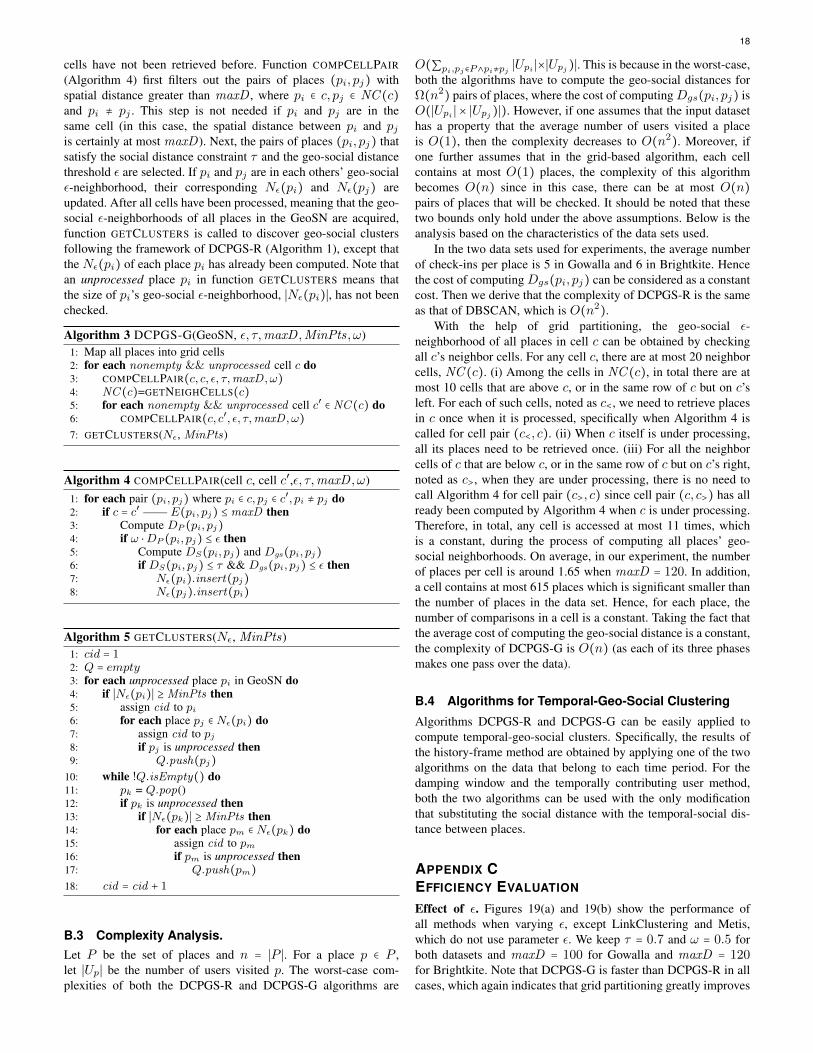
18

cells have not been retrieved before. Function COMPCELLPAIR

(Algorithm 4) first filters out the pairs of places (pi, pj) withspatial distance greater than maxD , where pi ∈ c, pj ∈ NC (c)and pi ≠ pj . This step is not needed if pi and pj are in thesame cell (in this case, the spatial distance between pi and pjis certainly at most maxD). Next, the pairs of places (pi, pj) thatsatisfy the social distance constraint τ and the geo-social distancethreshold ε are selected. If pi and pj are in each others’ geo-socialε-neighborhood, their corresponding Nε(pi) and Nε(pj) areupdated. After all cells have been processed, meaning that the geo-social ε-neighborhoods of all places in the GeoSN are acquired,function GETCLUSTERS is called to discover geo-social clustersfollowing the framework of DCPGS-R (Algorithm 1), except thatthe Nε(pi) of each place pi has already been computed. Note thatan unprocessed place pi in function GETCLUSTERS means thatthe size of pi’s geo-social ε-neighborhood, ∣Nε(pi)∣, has not beenchecked.

Algorithm 3 DCPGS-G(GeoSN, ε, τ,maxD ,MinPts, ω)1: Map all places into grid cells2: for each nonempty && unprocessed cell c do3: COMPCELLPAIR(c, c, ε, τ,maxD , ω)4: NC (c)=GETNEIGHCELLS(c)5: for each nonempty && unprocessed cell c′ ∈ NC (c) do6: COMPCELLPAIR(c, c′, ε, τ,maxD , ω)

7: GETCLUSTERS(Nε, MinPts)

Algorithm 4 COMPCELLPAIR(cell c, cell c′,ε, τ,maxD , ω)1: for each pair (pi, pj) where pi ∈ c, pj ∈ c′, pi ≠ pj do2: if c = c′ —— E(pi, pj) ≤ maxD then3: Compute DP (pi, pj)4: if ω ⋅DP (pi, pj) ≤ ε then5: Compute DS(pi, pj) and Dgs(pi, pj)6: if DS(pi, pj) ≤ τ && Dgs(pi, pj) ≤ ε then7: Nε(pi).insert(pj)8: Nε(pj).insert(pi)

Algorithm 5 GETCLUSTERS(Nε, MinPts)1: cid = 12: Q = empty3: for each unprocessed place pi in GeoSN do4: if ∣Nε(pi)∣ ≥MinPts then5: assign cid to pi6: for each place pj ∈ Nε(pi) do7: assign cid to pj8: if pj is unprocessed then9: Q.push(pj)

10: while !Q.isEmpty() do11: pk = Q.pop()12: if pk is unprocessed then13: if ∣Nε(pk)∣ ≥MinPts then14: for each place pm ∈ Nε(pk) do15: assign cid to pm16: if pm is unprocessed then17: Q.push(pm)

18: cid = cid + 1

B.3 Complexity Analysis.Let P be the set of places and n = ∣P ∣. For a place p ∈ P ,let ∣Up∣ be the number of users visited p. The worst-case com-plexities of both the DCPGS-R and DCPGS-G algorithms are

O(∑pi,pj∈P∧pi≠pj ∣Upi ∣×∣Upj)∣. This is because in the worst-case,both the algorithms have to compute the geo-social distances forΩ(n2) pairs of places, where the cost of computingDgs(pi, pj) isO(∣Upi ∣ × ∣Upj)∣). However, if one assumes that the input datasethas a property that the average number of users visited a placeis O(1), then the complexity decreases to O(n2). Moreover, ifone further assumes that in the grid-based algorithm, each cellcontains at most O(1) places, the complexity of this algorithmbecomes O(n) since in this case, there can be at most O(n)pairs of places that will be checked. It should be noted that thesetwo bounds only hold under the above assumptions. Below is theanalysis based on the characteristics of the data sets used.

In the two data sets used for experiments, the average numberof check-ins per place is 5 in Gowalla and 6 in Brightkite. Hencethe cost of computing Dgs(pi, pj) can be considered as a constantcost. Then we derive that the complexity of DCPGS-R is the sameas that of DBSCAN, which is O(n2).

With the help of grid partitioning, the geo-social ε-neighborhood of all places in cell c can be obtained by checkingall c’s neighbor cells. For any cell c, there are at most 20 neighborcells, NC (c). (i) Among the cells in NC (c), in total there are atmost 10 cells that are above c, or in the same row of c but on c’sleft. For each of such cells, noted as c<, we need to retrieve placesin c once when it is processed, specifically when Algorithm 4 iscalled for cell pair (c<, c). (ii) When c itself is under processing,all its places need to be retrieved once. (iii) For all the neighborcells of c that are below c, or in the same row of c but on c’s right,noted as c>, when they are under processing, there is no need tocall Algorithm 4 for cell pair (c>, c) since cell pair (c, c>) has allready been computed by Algorithm 4 when c is under processing.Therefore, in total, any cell is accessed at most 11 times, whichis a constant, during the process of computing all places’ geo-social neighborhoods. On average, in our experiment, the numberof places per cell is around 1.65 when maxD = 120. In addition,a cell contains at most 615 places which is significant smaller thanthe number of places in the data set. Hence, for each place, thenumber of comparisons in a cell is a constant. Taking the fact thatthe average cost of computing the geo-social distance is a constant,the complexity of DCPGS-G is O(n) (as each of its three phasesmakes one pass over the data).

B.4 Algorithms for Temporal-Geo-Social Clustering

Algorithms DCPGS-R and DCPGS-G can be easily applied tocompute temporal-geo-social clusters. Specifically, the results ofthe history-frame method are obtained by applying one of the twoalgorithms on the data that belong to each time period. For thedamping window and the temporally contributing user method,both the two algorithms can be used with the only modificationthat substituting the social distance with the temporal-social dis-tance between places.

APPENDIX CEFFICIENCY EVALUATION

Effect of ε. Figures 19(a) and 19(b) show the performance ofall methods when varying ε, except LinkClustering and Metis,which do not use parameter ε. We keep τ = 0.7 and ω = 0.5 forboth datasets and maxD = 100 for Gowalla and maxD = 120for Brightkite. Note that DCPGS-G is faster than DCPGS-R in allcases, which again indicates that grid partitioning greatly improves

19

the efficiency of DCPGS. DCPGS-G (DCPGS-R) is slightly moreexpensive than Jaccard-G (Jaccard-R). The runtimes of SimRank-G, SimRank-R, Katz-G, and CommuteTime-G increase signifi-cantly when ε increases from 0.1 to 0.5, because the increaseweakens the power of the spatial filter (Proposition 1) and more(expensive) social distances (Dsim

S (pi, pj), DKatzS (pi, pj), and

DctS (pi, pj)) are computed. DCPGS-G and DCPGS-R remain

quite stable for all ε values since the computational cost of oursocial distance is insignificant.Effect of maxD (eps in DBSCAN). Parameter maxD (eps inDBSCAN) decides the spatial ranges of the geo-social (spatial)neighborhoods of places and the size of the constructed placenetwork for LinkClustering and Metis. Thus, maxD (eps) greatlyinfluences the efficiency of all methods. Figures 19(c) and 19(d)display the runtime of all methods when varying maxD (eps).We set τ = 0.7, ε = 0.4, and ω = 0.5 for all the methodsexcept DBSCAN on both Gowalla and Brightkite datasets. Notethat SimRank-G, SimRank-R, Katz-G and CommuteTime-G aremore sensitive to maxD compared to the other methods, due tothe high cost of Dsim

S (pi, pj), DKatzS (pi, pj), and Dct

S (pi, pj)distance computations.

The cost of DCPGS-G stays below 100 seconds as maxDranges from 10 to 300 and remains close to that of DBSCAN-G and Jaccard-G. DCPGS-R is also close to DBSCAN-R andJaccard-R. DCPGS-G remains faster than DCPGS-R, but theirperformance gap narrows with maxD ; the reason is that grid-based computations become more expensive as the grid cell size(i.e., maxD) increases. DCPGS-R eventually becomes faster thanDCPGS-G for a very large maxD , e.g. maxD > 1000; however,as shown in Figure 2(c), geo-social clusters with a very largemaxD are not spatially identifiable. At an appropriate maxDvalue (around 100), DCPGS-G is clearly the best choice. Metishas similar cost to DCPGS-G while LinkClustering is slower.Effect of ω. Figures 19(e) and 19(f) display the runtimes of theclustering methods when varying ω. We keep τ = 0.7 and ε = 0.4for all methods on both datasets, while setting maxD = 100 inGowalla and maxD = 120 in Brightkite. The costs of all methodsare not much sensitive to ω; an exception is the runtimes ofSimRank-G, SimRank-R, Katz-G, and CommuteTime-G whichdecrease when ω > 0.5. The reason is again the high effect ofthe spatial filter (Proposition 1), when ω is large, due to whichmany expensive social distance computations are avoided. As afinal note, the social distance constraint τ is only applied as anultimate filter and has no influence on the runtimes of all methods.It only slightly influences the costs of LinkClustering and Metisbecause it affects the size of the place network, on which thesemethods operate.

▷ DCPGS-G * DCPGS-R ◁ Katz-G+ DBSCAN-G ◻ DBSCAN-R CommuteTime-G SimRank-G × SimRank-R ∎ Jaccard-G# LinkClustering Metis Jaccard-R

0.1 0.2 0.3 0.4 0.5 0.6 0.7 0.8 0.9 110

0

101

102

103

104

105

ε

Run

time

( se

cond

s )

(a) Gowalla0.1 0.2 0.3 0.4 0.5 0.6 0.7 0.8 0.9 1

100

101

102

ε

Run

time

( se

cond

s )

(b) Brightkite

10 50 100 150 200 250 30010

0

101

102

103

104

105

Run

time

( se

cond

s )

(DBSCAN) or (others)eps maxDm

(c) Gowalla

10 50 100 150 200 250 30010

0

101

102

103

Run

time

( se

cond

s )

(DBSCAN) or (others)eps maxDm

(d) Brightkite

0 0.1 0.2 0.3 0.4 0.5 0.6 0.7 0.8 0.9 110

1

102

103

104

105

ω

Run

time

( se

cond

s )

(e) Gowalla0 0.1 0.2 0.3 0.4 0.5 0.6 0.7 0.8 0.9 1

100

101

102

ω

Run

time

( se

cond

s )

(f) Brightkite

Fig. 19. Runtime experiments