1 detecting changes between optical images of … · detecting changes between optical images of...

1

Detecting Changes Between Optical Images

of Different Spatial and Spectral Resolutions:

a Fusion-Based ApproachVinicius Ferraris, Nicolas Dobigeon, Senior Member, IEEE,

Qi Wei, Member, IEEE, and Marie Chabert

Abstract

Change detection is one of the most challenging issues when analyzing remotely sensed images.

Comparing several multi-date images acquired through the same kind of sensor is the most common

scenario. Conversely, designing robust, flexible and scalable algorithms for change detection becomes

even more challenging when the images have been acquired by two different kinds of sensors. This

situation arises in case of emergency under critical constraints. This paper presents, to the best of

authors’ knowledge, the first strategy to deal with optical images characterized by dissimilar spatial

and spectral resolutions. Typical considered scenarios include change detection between panchromatic

or multispectral and hyperspectral images. The proposed strategy consists of a 3-step procedure:

i) inferring a high spatial and spectral resolution image by fusion of the two observed images

characterized one by a low spatial resolution and the other by a low spectral resolution, ii) predicting

two images with respectively the same spatial and spectral resolutions as the observed images by

degradation of the fused one and iii) implementing a decision rule to each pair of observed and

predicted images characterized by the same spatial and spectral resolutions to identify changes. The

performance of the proposed framework is evaluated on real images with simulated realistic changes.

Index Terms

Change detection, Image fusion, Different resolution, Hyperspectral imagery, Multispectral im-

agery.

Part of this work has been supported by Coordenação de Aperfeiçoamento de Ensino Superior (CAPES), Brazil, and EU

FP7 through the ERANETMED JC-WATER Program, MapInvPlnt Project ANR-15-NMED-0002-02.

V. Ferraris, N. Dobigeon and M. Chabert are with University of Toulouse, IRIT/INP-ENSEEIHT, France (email:

vinicius.ferraris, nicolas.dobigeon, [email protected]).

Q. Wei is with Department of Engineering, University of Cambridge, CB2 1PZ, Cambridge, UK (email:

[email protected]).

September 21, 2016 DRAFT

arX

iv:1

609.

0607

4v1

[cs

.CV

] 2

0 Se

p 20

16

2

I. INTRODUCTION

Change detection (CD) is one of the most investigated issues in remote sensing [1]–[4]. As the

name suggests, it consists in analyzing two or more multi-date (i.e., acquired at different time instants)

images of the same scene to detect potential changes. Applications are diverse, from natural disaster

monitoring to long-term tracking of urban and forest growth. Optical images have been the most

studied remote sensing data for CD. They are generally well suited to map land-cover types at

large scales [5]. Multi-band optical sensors use a spectral window with a particular width, often

called spectral resolution, to sample part of the electromagnetic spectrum of the incoming light. The

term spectral resolution can also refer to the number of spectral bands and multi-band images can

be classified according to this number [6], [7]. Panchromatic (PAN) images are characterized by a

low spectral resolution, sensing part of the electromagnetic spectrum with a single and generally

wide spectral window. Conversely, multispectral (MS) and hyperspectral (HS) images have smaller

spectral windows, allowing part of the spectrum to be sensed with higher precision. Multi-band optical

imaging has become a very common modality of remote sensing, boosted by the advent of new finer

spectral sensors [8]. One of the major advantages of multi-band images is the possibility of detecting

changes by exploiting not only the spatial but also the spectral information. There is no specific

convention regarding the numbers of bands that characterize MS and HS images. Yet, MS images

generally consists of a dozen of spectral bands while HS may have a lot more than a hundred. In

complement to spectral resolution taxonomy, one may describe multi-band images in terms of their

spatial resolution measured by the ground sampling interval (GSI), e.g. the distance, on the ground,

between the center of two adjacent pixels [5], [7], [9]. Informally, it represents the smallest object

that can be resolved up to a specific pixel size. Then, the higher the resolution, the smaller the

recognizable details on the ground: a high resolution (HR) image has smaller GSI and finer details

than a low resolution (LR) one, where only coarse features are observable. Each image sensor is

designed based on a particular signal-to-noise ratio (SNR). The reflected incoming light must be of

sufficient energy to guarantee a sufficient SNR and thus a proper acquisition. To increase the energy

level of the arriving signal, either the instantaneous field of view (IFOV) or the spectral window width

must be increased. However these solutions are mutually exclusive. In other words, optical sensors

suffer from an intrinsic energy trade-off that limits the possibility of acquiring images of both high

spatial and high spectral resolutions [9], [10]. This trade-off prevents any simultaneous decrease of

both the GSI and the spectral window width. Consequently, as an archetypal example, HS images

are generally of lower spatial resolution than MS and PAN images.

Because of the common assumption of an additive Gaussian noise model for passive optical

images, the most common CD techniques designed for single-band optical images are based on image


3

differencing [1]–[4]. When dealing with multi-band images, classical CD differencing methods have

been adapted for such data through spectral change vectors [2], [11], [12] or transform analysis [13],

[14]. Besides, most CD techniques assume that the multi-date images have been acquired by sensors of

the same type [4] with similar acquisition characteristics in terms of, e.g., angle-of-view, resolutions or

noise model [15], [16]. Nevertheless, in some specific scenarios, for instance consecutive to natural

disasters, such a constraint may not be ensured, e.g., images compatible with previously acquired

ones may not be available in an acceptable timeframe. Such disadvantageous emergency situations

yet require fast, flexible and accurate methods able to handle images acquired by sensors of different

kinds [17]–[22]. Facing with heterogeneity of data is a challenging task and must be carefully handled.

However, since CD techniques for optical images generally rely on the assumption of data acquired

by similar sensors, suboptimal strategies have been considered to make these techniques applicable

when considering optical images of different spatial and spectral resolutions [13], [18]. In particular,

interpolation and resampling are classically used to obtain a pair of images with the same spatial

and spectral resolutions [18], [23]. However, such a compromise solution may remain suboptimal

since it considers each image individually without fully exploiting their joint characteristics and their

complementarity. In this paper, we address the problem of unsupervised CD technique of multi-band

optical images with different spatial and spectral resolutions. To the best of authors’ knowledge, this

is the first operational framework specifically designed to address this issue.

More precisely, this paper addresses the problem of CD between a pair of optical images acquired

over the same scene at different time instants, one with low spatial and high spectral resolutions and

one with high spatial and low spectral resolutions. The proposed approach consists in first fusing the

two observed images. The result would be a high spatial and high spectral resolution image of the

observed scene as if the two observed images were acquired at the same time or, in our case of study,

if no change occurred between the two acquisition times. Otherwise, the result does not correspond to

a truly observed scene but it contains the change information. The proposed fusion process explicitly

relies on a physically-based sensing model which exploits the characteristics of the two sensors,

following the frameworks in [24], [25]. These characteristics are subsequently resorted to obtain, by

degradation of the fusion result, two so-called predicted images with the same resolutions as the

observed images, i.e., one with low spatial resolution and high spectral resolutions and one with high

spatial resolution and low spectral resolutions. In absence of any change, these two pairs of predicted

and observed images should coincide, apart from residual fusion errors/inacurracies. Conversely, any

change between the two observed images is expected to produce spatial and/or spectral alterations in

the fusion result, which will be passed on the predicted images. Finally, each predicted image can

be compared to the corresponding observed image of same resolution to identify possible changes.

Since for each pair, the images to be compared are of the same resolution, classical CD methods


4

dedicated to multi-band image can be considered [3], [4]. The final result is composed of two change

detection maps with two different spatial resolutions.

The paper is organized as follows. Section II introduces the proposed change detection framework,

which is composed of three main steps: fusion, prediction and decision. The first two steps are

described in Section III which introduces the forward model underlying the observation process.

Section IV, dedicated to the third step, discusses three CD techniques operating on mono- and/or

multi-band images of identical spatial and spectral resolutions. Experimental results are provided in

Section V, where a specific simulation protocol is detailed. These results demonstrate the efficiency

of the proposed CD framework. Section VI concludes this paper.

II. PROPOSED CHANGE DETECTION FRAMEWORK

Lets us denote t1 and t2 the times of acquisition for two multi-band optical images over the same

scene of interest. Assume that the image acquired at time t1 is a high spatial resolution PAN or MS

(HR-PAN/MS) image denoted as Yt1HR ∈ Rnλ×n and the one acquired at time t2 is a low spatial

resolution HS (LR-HS) image denoted as Yt2LR ∈ Rmλ×m, where

• n = nr × nc is the number of pixels in each band of the HR-PAN/MS image,

• m = mr ×mc is the number of pixels in each band of the LR-HS image, with m < n,

• nλ is the number of bands in the HR-PAN/MS image,

• mλ is the number of bands in the LR-HS image, with nλ < mλ.

The main difficulty which prevents any naive implementation of classical CD methods results from the

differences in spatial and spectral resolutions of the two observed images, i.e., m 6= n and nλ 6= mλ.

Besides, in digital image processing, it is common to consider the image formation process as a

sequence of transformations of the original scene into an output image. The output image of a given

sensor is thus a particular limited representation of the original scene with characteristics imposed

by the processing pipeline of that sensor, called image signal processor (ISP). The original scene

cannot be exactly represented because of its continuous nature. Nevertheless, to represent the ISP

pipeline as a sequence of transformations, it is usual to consider a very fine digital approximation of

the scene representation as the input image. Following this paradigm, the two observed images Yt1HR

and Yt2LR are assumed to be spectrally and spatially degraded versions of two corresponding latent

(i.e., unobserved) high resolution hyperspectral images (HR-HS) Xt1 and Xt2 , respectively,

Yt1HR = THR

[Xt1]

Yt2LR = TLR

[Xt2] (1)

where THR [·] and TLR [·] stand for spectrally and spatially degradation operators and Xtj ∈ Rmλ×n

(j = 1, 2). Note that these two unobserved images Xtj ∈ Rmλ×n (j = 1, 2) share the same spatial


5

and spectral characteristics and, if they were available, they could be resorted as inputs of classical

CD techniques operating on images of same resolutions.

When the two images Yt1HR and Yt2

LR have been acquired at the same time, i.e., t1 = t2, no

change is expected and the latent images Xt1 and Xt2 should represent exactly the same scene, i.e.,

Xt1 = Xt2 , X. In such a particular context, recovering an estimate X of the HR-HS latent image

X from the two degraded images Yt1HR and Yt2

LR can be cast as a fusion problem, for which efficient

methods have been recently proposed [25]–[28]. Thus, in the case of a perfect fusion process, the

no-change hypothesis H0 can be formulated as

H0 :

Yt1HR = Yt1

HR

Yt2LR = Yt2

LR

(2)

whereYt1

HR , THR

[X]

Yt2LR , TLR

[X] (3)

are the two predicted HR-PAN/MS and LR-HS images from the estimated HR-HS latent image X.

When there exists a time interval between acquisitions, i.e. when t1 6= t2, a change may occur

meanwhile. In this case, no common latent image X can be defined since Xt1 6= Xt2 . However, since

Xt1 and Xt2 represent the same area of interest, they are expected to keep a certain level of similarity.

Thus, the fusion process does not lead to a common latent image, but to a pseudo-latent image X

from the observed image pair Yt1HR and Yt2

LR, which consists of the best joint approximation of latent

images Xt1 and Xt2 . Moreover, since X 6= Xt1 and X 6= Xt2 , the forward model (1) does not hold to

relate the pseudo-latent image X to the observations Yt1HR and Yt2

LR. More precisely, when changes

have occurred between the two time instants t1 and t2, the change hypothesis H1 can be stated as

H1 :

Yt1HR 6= Yt1

HR

Yt2LR 6= Yt2

LR.(4)

More precisely, both inequalities in (4) should be understood in a pixel-wise sense since any change

occurring between t1 and t2 is expected to affect some spatial locations in the images. As a conse-

quence, both diagnosis in (2) and (4) naturally induce pixel-wise rules to decide between the no-change

and change hypothesis H0 and H1. This work specifically proposes to derive a CD technique able

to operate on the two observed images Yt1HR and Yt2

LR. It mainly consists of a the following 3-steps,

sketched in Fig. 1

1) fusion: estimating the HR-HS pseudo-latent image X from Yt1HR and Yt2

LR,

2) prediction: reconstructing the two HR-PAN/MS and LR-HS images Yt1HR and Yt2

LR from X,

3) decision: deriving HR and LR change maps DHR and DLR associated with the respective pairs


6

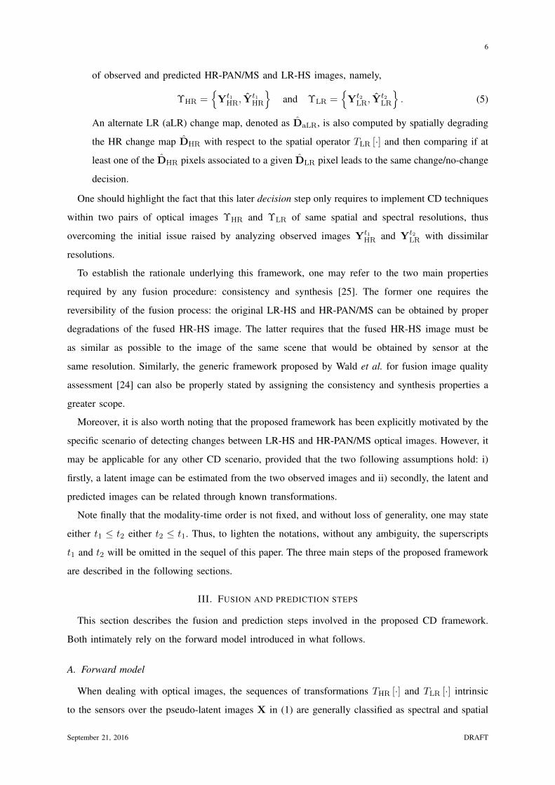
of observed and predicted HR-PAN/MS and LR-HS images, namely,

ΥHR =

Yt1HR, Y

t1HR

and ΥLR =

Yt2

LR, Yt2LR

. (5)

An alternate LR (aLR) change map, denoted as DaLR, is also computed by spatially degrading

the HR change map DHR with respect to the spatial operator TLR [·] and then comparing if at

least one of the DHR pixels associated to a given DLR pixel leads to the same change/no-change

decision.

One should highlight the fact that this later decision step only requires to implement CD techniques

within two pairs of optical images ΥHR and ΥLR of same spatial and spectral resolutions, thus

overcoming the initial issue raised by analyzing observed images Yt1HR and Yt2

LR with dissimilar

resolutions.

To establish the rationale underlying this framework, one may refer to the two main properties

required by any fusion procedure: consistency and synthesis [25]. The former one requires the

reversibility of the fusion process: the original LR-HS and HR-PAN/MS can be obtained by proper

degradations of the fused HR-HS image. The latter requires that the fused HR-HS image must be

as similar as possible to the image of the same scene that would be obtained by sensor at the

same resolution. Similarly, the generic framework proposed by Wald et al. for fusion image quality

assessment [24] can also be properly stated by assigning the consistency and synthesis properties a

greater scope.

Moreover, it is also worth noting that the proposed framework has been explicitly motivated by the

specific scenario of detecting changes between LR-HS and HR-PAN/MS optical images. However, it

may be applicable for any other CD scenario, provided that the two following assumptions hold: i)

firstly, a latent image can be estimated from the two observed images and ii) secondly, the latent and

predicted images can be related through known transformations.

Note finally that the modality-time order is not fixed, and without loss of generality, one may state

either t1 ≤ t2 either t2 ≤ t1. Thus, to lighten the notations, without any ambiguity, the superscripts

t1 and t2 will be omitted in the sequel of this paper. The three main steps of the proposed framework

are described in the following sections.

III. FUSION AND PREDICTION STEPS

This section describes the fusion and prediction steps involved in the proposed CD framework.

Both intimately rely on the forward model introduced in what follows.

A. Forward model

When dealing with optical images, the sequences of transformations THR [·] and TLR [·] intrinsic

to the sensors over the pseudo-latent images X in (1) are generally classified as spectral and spatial


7

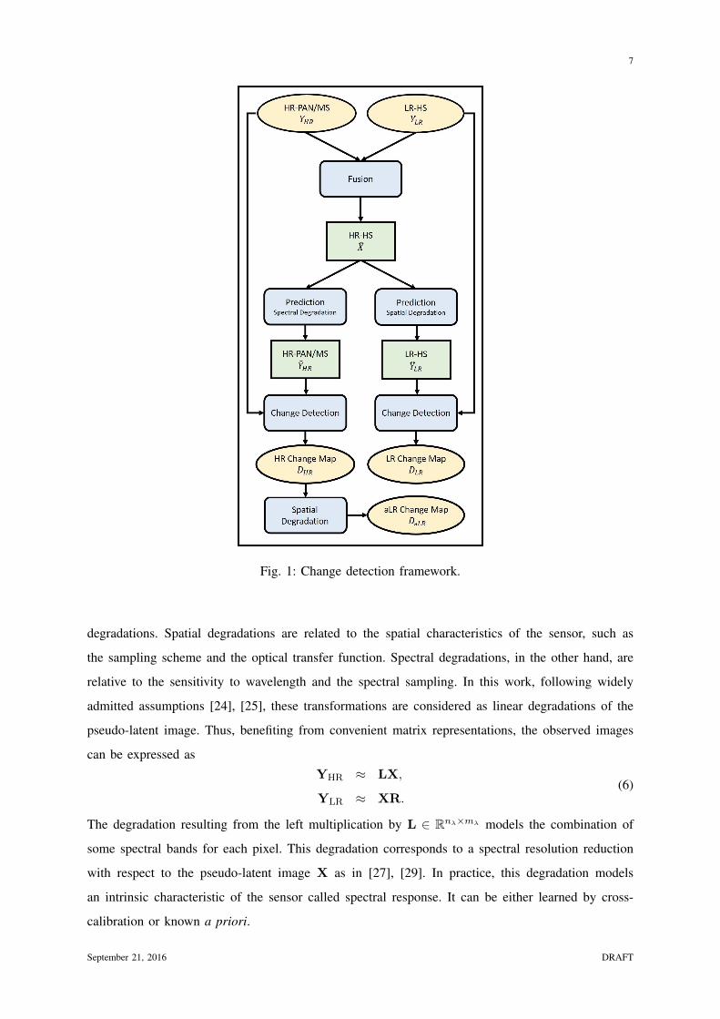
Fig. 1: Change detection framework.

degradations. Spatial degradations are related to the spatial characteristics of the sensor, such as

the sampling scheme and the optical transfer function. Spectral degradations, in the other hand, are

relative to the sensitivity to wavelength and the spectral sampling. In this work, following widely

admitted assumptions [24], [25], these transformations are considered as linear degradations of the

pseudo-latent image. Thus, benefiting from convenient matrix representations, the observed images

can be expressed asYHR ≈ LX,

YLR ≈ XR.(6)

The degradation resulting from the left multiplication by L ∈ Rnλ×mλ models the combination of

some spectral bands for each pixel. This degradation corresponds to a spectral resolution reduction

with respect to the pseudo-latent image X as in [27], [29]. In practice, this degradation models

an intrinsic characteristic of the sensor called spectral response. It can be either learned by cross-

calibration or known a priori.


8

Conversely, the right multiplication by R ∈ Rn×m degrades the pseudo-latent image by linear

combinations of pixels within a given spectral band, thus reducing the spatial resolution. The right

degradation matrix R may model the combination of various transformations which are specific

of sensor architectures and take into account external factors such as wrap, blurring, translation,

decimation, etc [27], [29], [30]. In this work, only space invariant blurring and decimation will

be considered. Geometrical transformations such as wrap and translations can be corrected using

image co-registration techniques in pre-processing steps. A space-invariant blur can be modeled by

a symmetric convolution kernel, yielding a sparse symmetric Toeplitz matrix B ∈ Rn×n [26]. It

operates a cyclic convolution on the image bands individually. The decimation operation S ∈ Rn×m

corresponds to a d = dr × dc uniform downsampling1 operator with m = n/d ones on the block

diagonal and zeros elsewhere, such that STS = Im [27]. Hence, the spatial degradation operation

corresponds to the composition R = BS ∈ Rn×m.

The approximating symbol ≈ in (6) stands for any mismodeling effects or acquisition noise, which

is generally considered as additive and Gaussian [4], [9], [25]–[28]. The full degradation model can

thus be written asYHR = LX + NHR,

YLR = XBS + NLR.(7)

The additive noise matrices are assumed to be distributed according to matrix normal distributions2

[31], as followsNHR ∼MNmλ,m(0mλ×m,ΛHR, Im),

NLR ∼MNnλ,n(0nλ×n,ΛLR, In).

Note that the row covariance matrices ΛHR and ΛLR carry the information of the spectral variance

in-between bands. Since the noise is spectrally colored, these matrices are not necessarily diagonal.

In the other hand, since the noise is assumed spatially independent, the column covariance matrices

correspond to identity matrices, e.g., Im and In. In real applications, since the row covariance matrices

are an intrinsic characteristic of the sensor, they are estimated by a prior calibration [29]. In this paper,

to reduce the number of unknown parameters we assume that ΛHR and ΛLR are both diagonal. This

1The inverse downsampling transformation ST represent an upsampling transformation by zero interpolation from m to

n.2The probability density function, p(X|M,Σr,Σr) of a matrix normal distribution MNr,c(M,Σr,Σc) is given by

p (X|M,Σr,Σr) =exp

(− 1

2tr[Σ−1c (X−M)T Σ−1

r (X−M)])

(2π)rc/2 |Σc|r/2 |Σr|c/2

where M ∈ Rr×c is the mean matrix, Σr ∈ Rr×r is the row covariance matrix and Σc ∈ Rc×c is the column covariance

matrix.


9

hypothesis implies that the noise is independent from one band to another and is characterized by a

specific variance in each band [27].

B. Fusion process

The forward observation model (7) has been exploited in many applications involving optical multi-

band images, specially those related to image restoration such as fusion and superresolution [27], [29].

Whether the objective is to fuse multi-band images from different spatial and spectral resolutions or

to increase the resolution of a single one, it consists in compensating the energy trade-off of optical

multi-band sensors to get a higher spatial and spectral resolution image compared to the observed

image set. One popular approach to conduct fusion consists in solving an inverse problem, formulated

through the observation model. In the specific context of HS pansharpening (i.e., fusing PAN and HS

images), such an approach has proven to provide the most reliable fused product, with a reasonable

computational complexity [25]. For these reasons, this is the strategy followed in this work and it is

briefly sketched in what follows.

Because of the additive nature and the statistical properties of the noise NHR and NLR, both

observed images YHR and YLR are assumed to be distributed according to matrix normal distributions

YHR|X ∼MNmλ,m(LX,ΛHR, Im)

YLR|X ∼MNnλ,n(XBS,ΛLR, In)(8)

Since the noise can be reasonably assumed sensor-dependent, the observed images can be assumed

statistically independent. Consequently the joint likelihood function of the statistical independent

observed data can be written

p(YHR,YLR|X) = p(YHR|X)p(YLR|X) (9)

and the negative log-likelihood, defined up to an additive constant, is

− log p(Ψ|X) =1

2

∥∥∥Λ− 1

2

HR (YHR − LX)∥∥∥2

F

+1

2

∥∥∥Λ− 1

2

LR (YLR −XBS)∥∥∥2

F

(10)

where Ψ = YHR,YLR denotes the set of observed images and ‖·‖2F stands for the Frobenius norm.

Computing the maximum likelihood estimator XML of X from the observed image set Ψ consists

in minimizing (10). The aforementioned derivation intents to solve a linear inverse problem which

can be ill-posed or ill-conditioned, according to the properties of the matrices B, S and L defining

the forward model (7). To overcome this issue, additional prior information can be included, setting

the estimation problem into the Bayesian formalism [32]. Following a maximum a posteriori (MAP)

estimation, recovering the estimated pseudo-latent image X from the linear model (7) consists in


10

minimizing the negative log-posterior

X ∈ argminX∈Rmλ×n

1

2

∥∥∥Λ− 1

2

HR (YHR − LX)∥∥∥2

F

+1

2

∥∥∥Λ− 1

2

LR (YLR −XBS)∥∥∥2

F+ λφ(X)

(11)

where φ(·) defines an appropriate regularizer derived from the prior distribution assigned to X and

λ is a parameter that tunes the relative importance of the regularization and data terms. Computing

the MAP estimator (11) is expected to provide the best approximation X with the minimum distance

to the latent images Xt1 and Xt2 simultaneously. This optimization problem is challenging because

of the high dimensionality of the data X. Nevertheless, Wei et al. [27] has proved that its solution

can be efficiently computed for various relevant regularization terms φ(X). In this work, a Gaussian

prior is considered, since it provides an interesting trade-off between accuracy and computational

complexity, as reported in [25].

C. Prediction

The prediction step relies on the forward model (7) proposed in Section III-A. As suggested by

(3), it merely consists in applying the respective spectral and spatial degradations to the estimated

pseudo-latent image X, leading toYHR = LX

YLR = XBS.(12)

IV. OPTICAL IMAGE HOMOGENEOUS CHANGE DETECTION

This section presents the third and last step of the proposed CD framework, which consists in

implementing decision rules to identify possible changes between the images composing the two

pairs ΥHR =

YHR, YHR

and ΥLR =

YLR, YLR

. As noticed in Section II, these CD techniques

operate on observed Y·R and predicted Y·R images of same spatial and spectral resolutions, with

· ∈ H,L, as in [2], [3], [33], [34]. Unless explicitly specified, they can be employed whatever the

number of bands. As a consequence, Y·R and Y·R could refer to either PAN, MS or HS images and

the two resulting CD maps are either of HR, either of LR, associated with the pairs ΥHR and ΥLR,

respectively. To lighten the notations, without loss of generality, in what follows, the pairs Y·R and

Y·R will be denoted Y1 ∈ R`×η and Y2 ∈ R`×η, which can be set as

• Y1,Y2 = ΥLR to derive the estimated CD binary map DLR at LR,

• Y1,Y2 = ΥHR to derive the estimated CD binary map DHR at HR and its spatially degraded

aLR counterpart DaLR.

In this seek of generality, the numbers of bands and pixels are denoted ` and η, respectively. The

spectral dimension ` depends on the considered image sets ΥHR or ΥLR, i.e., ` = nλ and ` = mλ for


11

HR and LR images, respectively3. Similarly, the spatial resolution of the CD binary map generically

denoted as D ∈ Rη depends on the considered set of images ΥHR or ΥLR, i.e., η = n and η = m

for HR and LR images, respectively.

Three efficient CD techniques operating on images of same spatial and spectral resolutions are

discussed below.

A. Change vector analysis (CVA)

When considering multi-band optical images after atmospheric and geometric pre-calibration, for

a pixel at spatial location p = (ip, jp), one may consider that

Y1(p) ∼ N (µ1,Σ1)

Y2(p) ∼ N (µ2,Σ2)(13)

where µ1 ∈ R` and µ2 ∈ R` correspond to the pixel spectral mean and Σ1 ∈ R`×` and Σ2 ∈ R`×` are

the spectral covariance matrices (here they were obtained using the maximum likelihood estimator).

The spectral change vector is defined by the squared Mahalanobis distance between the two pixels

which can be computed from the pixel-wise spectral difference operator ∆Y(p) = Y1(p) −Y2(p),

i.e.,

VCVA(p) = ‖∆Y(p)‖2Σ−1 = ∆Y(p)TΣ−1∆Y(p) (14)

where Σ = Σ1 + Σ2. For a given threshold τ , the pixel-wise statistical test can be formulated as

VCVA(p)H1

≷H0

τ (15)

and the final CD map, denoted DCVA ∈ 0, 1η can be derived as

DCVA(p) =

1 if VCVA(p) ≥ τ (H1)

0 otherwise (H0).(16)

For a pixel which has not been affected by a change (hypothesis H0), the spectral difference operator

is expected to be statistically described by ∆Y(p) ∼ N (0,Σ). As a consequence, the threshold τ

can be related to the probability of false alarm (PFA) of the test

PFA = P[VCVA(p) > τ

∣∣∣∣H0

](17)

or equivalently,

τ = F−1χ2`

(1− PFA) (18)

where F−1χ2`(·) is the inverse cumulative distribution function of the χ2

` distribution.

3Note, in particular, that ` = nλ = 1 when the set of HR images are PAN images.


12

B. Spatially regularized change vector analysis

Since CVA in its simplest form as presented in Section IV-A is a pixel-wise procedure, it sig-

nificantly suffers from low robustness with respect to noise. To overcome this limitation, spatial

information can be exploited by considering the neighborhood of a pixel to compute the final distance

criterion, which is expected to make the change map spatially smoother. Indeed, changed pixels are

generally gathered together into regions or clusters, which means that there is a high probability to

observe changes in the neighborhood of an identified changed pixel [3]. Let ΩLp denote the set of

indexes of neighboring spatial locations of a given pixel p defined by a surrounding regular window

of size L centered on p. The spatially smoothed energy map VsCVA of the spectral difference operator

can be derived from its pixel-wise counterpart VCVA defined by (14) as

VsCVA(p) =1

|ΩLp |∑k∈ΩLp

ω(k)VCVA(k) (19)

where the weights ω(k) ∈ R|ΩLp | implicitly define a spatial smoothing filter. In this work, they are

chosen as ω(k) = 1, ∀k ∈

1, . . . , |ΩLp |

. Then, a decision rule similar to (16) can be followed to

derive the final CD map DsCVA. Note, the choice of window size L is based on the strong hypothesis

of the window homogeneity. This choice thus may depend upon the kind of observed scenes.

C. Iteratively-reweighted multivariate alteration detection (IR-MAD)

The multivariate alteration detection (MAD) technique introduced in [13] has been shown to be

a robust CD method due to being well suited for analyzing multi-band image pair Y1,Y2 with

possible different intensity levels. Similarly to the CVA and sCVA methods, it exploits an image

differencing operator while better concentrating information related to changes into auxiliary variables.

More precisely, the MAD variate is defined as ∆Y(p) = Y1(p)− Y2(p) with

Y1(p) = UY1(p)

Y2(p) = VY2(p)

(20)

where U = [u`,u`−1, . . . ,u1]T is a ` × `-matrix composed of the ` × 1-vectors uj identified by

canonical correlation analysis and V = [v`,v`−1, . . . ,v1]T is defined similarly. As in Equation (14),

the MAD-based change energy map can then be derived as

VMAD(p) = ‖∆Y(p)‖2Λ−1

where Λ is the diagonal covariance matrix of the MAD variates. Finally, the MAD CD map DMAD

can be pixel-wisely computed using a decision rule similar to (16) with a threshold τ related to the

PFA by (18). In this work, the iteratively re-weighted version of MAD (IR-MAD) has been considered

to better separate the change pixels from the no-change pixels [14].


13

V. EXPERIMENTS

This section assesses the performance of the proposed fusion-based CD framework. First, the

simulation protocol is described in Section V-A. Then, Section V-B reports qualitative and quantitative

results when detecting changes between HS and MS or PAN images.

A. Simulation protocol

Evaluating performances of CD algorithms requires image pairs with particular characteristics,

which makes them rarely freely available. Indeed, CD algorithms require images acquired at two

different dates, presenting changes, geometrically and radiometrically pre-corrected and, for the

specific problem addressed in this paper, coming from different optical sensor modes. Moreover,

these image pairs need to be accompanied by ground-truth information in the form of validated CD

mask.

To overcome this issue, this paper proposes to follow a strategy inspired by the protocol introduced

in [24] to assess the performance of pansharpening algorithms. This protocol relies on a unique

reference HS image Xref , also considered as HR. It avoids the need of co-registered and geometrically

corrected images by generating a pair of synthetic but realistic HR-PAN/MS and LR-HS images from

this reference image and by including changes within a semantic description of this HR-HS image.

In this work, this description is derived by spectral unmixing [35] and the full proposed protocol can

be summarized as follows:

i) Given an HR-HS reference image Xref ∈ Rmλ×n, conduct linear unmixing to extract K

endmember signatures Mt1 ∈ Rmλ×K and the associated abundance matrix At1 ∈ RK×n.

ii) Define the HR-HS latent image Xt1 before change as

Xt1 = Mt1At1 . (21)

iii) Define a reference HR change mask DHR by selecting particular regions (i.e., pixels) in the

HR-HS latent image Xt1 where changes occur. The corresponding LR change mask DLR is

computed according to the spatial degradations relating the two modalities. Both change masks

will be considered as the ground truth and will be compared to the estimated CD HR map DHR

and LR maps DLR and DaLR, respectively, to evaluate the performance of the proposed CD

technique.

iv) According to this reference HR change mask, implement realistic change rules on the reference

abundances At1 associated with pixels affected by changes. Several change rules applied to the

reference abundance will be discussed in Section V-A2. Note that theses rules may also require

the use of additional endmembers that are not initially present in the latent image Xt1 . The

abundance and endmember matrices after changes are denoted as At2 and Mt2 , respectively.


14

v) Define the HR-HS latent image Xt2 after changes by linear mixing such that

Xt2 = Mt2At2 . (22)

vi) Generate a simulated observed HR-PAN/MS image YHR by applying the spectral degradation

THR [·] either to the before-change HR-HS latent image Xt1 , either to the after-change HR-HS

latent image Xt2 .

vii) Conversely, generate a simulated observed LR-HS image YLR by applying the spatial degrada-

tion TLR [·] either to the after-change HR-HS latent image Xt2 , or to the before-change HR-HS

latent image Xt1 .

This protocol is illustrated in Fig. 2 and complementary information regarding these steps is

provided in the following paragraphs.

Fig. 2: Simulation protocol: two HR-HS latent images Xt1 (before changes) and Xt2 (after changes)

are generated from the reference image. In temporal configuration 1 (black), the observed HR-PAN/MS

image YHR is a spectrally degraded version of Xt1 while the observed LR-HS image Yt2LR is a

spatially degraded version of Xt2 . In temporal configuration 2 (grey dashed lines), the degraded

images are generated from reciprocal HR-HS images.


15

1) Reference image: The HR-HS reference image used in the simulation protocol is a 610 ×

330×115 HS image of the Pavia University in Italy acquired by the reflective optics system imaging

spectrometer (ROSIS) sensor. A pre-correction has been conducted to smooth the atmospheric effects

due to vapor water absorption by removing corresponding spectral bands. Then the final HR-HS

reference image is of size 610× 330× 93.

2) Generating the HR-HS latent images: unmixing, change mask and change rules: To produce the

HR-HS latent image Xt1 before change, the reference image Xref has been linearly unmixed, which

provides the endmember matrix Mt1 ∈ Rmλ×K and the matrix of abundances At1 ∈ RK×n where

K is the number of endmembers. This number K can be obtained by investigating the dimension

of the signal subspace, for instance by conducting principal component analysis [35]. In this work,

the linear unmixing has been conducted by coupling the vertex component analysis (VCA) [36] as

an endmember extraction algorithm and the fully constrained least squares (FCLS) algorithm [37] to

obtain Mt1 and At1 , respectively.

Given the HR-HS latent image Xt1 = Mt1At1 , the HR change mask DHR has been produced

by selecting spatial regions in the HR-HS image affected by changes. This selection can be made

randomly or by using prior knowledge on the scene. In this work, manual selection is performed.

Then, the change rules applied to the abundance matrix At1 to obtain the changed abundance

matrix At2 are chosen such that they satisfy the standard positivity and sum-to-one constraints

Nonnegativity at2k (p) ≥ 0,∀p ∈ 1, . . . , n ,∀k ∈ 1, . . . ,K

Sum-to-oneK∑k=1

at2k (p) = 1,∀p ∈ 1, . . . , n(23)

More precisely, three distinct change rules has been considered

• Zero abundance: find the most present endmember in the selected region, set all corresponding

abundances to zero and rescale abundances associated with remaining endmembers in order

to fulfill (23). This change can be interpreted as a brutal disappearing of the most present

endmember.

• Same abundance: choose a pixel abundance vector at random spatial location, set all abundance

vectors inside the region affected by changes to the chosen one. This change consists in filling

the change region by the same spectral signature.

• Block Abundance: randomly select a region with the same spatial shape of the region affected

by changes and replace original region abundances by the abundances of the second one. This

produce a “copy-paste” pattern.

Note that other change rules on the abundance matrix At1 could have been investigated; in particular

some of them could require to include additional endmembers in the initial endmember matrix Mt1 .


16

The updated abundance At2 and endmember Mt2 matrices allow to define the after-change HR-HS

latent image Xt2 as

Xt2 = Mt2At2 .

Fig. 3 shows the four different change rules for one single selected region in image.

(a) (b) (c) (d)

Fig. 3: Change rules applied to the reference image (a): (b) zero-abundance, (c) same abundance and

(d) block abundance.

3) Generating the observed images: spectral and spatial degradations: To produce spectrally

degraded versions YHR of the HR-HS latent image Xtj (j = 1 or j = 2), two particular spectral

responses have been used to assess the performance of the proposed algorithm when analyzing a

HR-PAN or a 4-band HR-MS image. The former has been obtained by uniformly averaging the first

43 bands of the HR-HS pixel spectra. The later has been obtained by filtering the HR-HS latent image

Xtj by a 4-band LANDSAT-like spectral response.

To generate a spatially degraded image, the HR-HS latent image Xtj (j = 2 or j = 1) has been

blurred by a 5×5 Gaussian kernel filter and down-sampled equally in vertical and horizontal directions

with a factor d = 5. This spatial degradation operator implicitly relates the generated HR change

mask DHR to its LR counterpart DLR. Each LR pixel contains d×d HR pixels. As DHR is a binary

mask, after the spatial degradation, if at least one of HR pixels associated to a given LR pixel is

considered as a change pixel then the pixel in DLR is also considered as a change pixel.

To illustrate the impact of these spectral and spatial degradations, Fig. 4 shows the HR-HS reference

Pavia University image (a), corresponding HR-PAN (b) and HR-MS (c) images resulting from spectral

degradations and a LR-HS image resulting from spatial degradation (d).

Note that, as mentioned in Section II, the modality-time order can be arbitrary fixed, and without

loss of generality, one may state either t1 ≤ t2 either t2 ≤ t1. Thus, there are 2 distinct temporal


17

(a) (b) (c)

Fig. 4: Degraded version of the reference image in Fig. 3(a): (a) spectrally degraded HR-PAN image,

(b) spectrally degraded HR-MS image and (c) spatially degraded LR-HS image.

configurations to generate the pair of observed HR and LR images:

• Configuration 1: generating the spectrally (resp., spatially) degraded observed image YHR (resp.,

YLR) from the before-change (resp., after-change) HR-HS latent image Xt1 (resp., Xt2),

• Configuration 2: generating the spectrally (resp., spatially) degraded observed image YHR (resp.,

YLR) from the after-change (resp., before-change) HR-HS latent image Xt2 (resp., Xt1).

B. Results

The CD framework introduced in Section II has been evaluated following the simulation protocol

described in the previous paragraph. More precisely, 75 regions have been randomly selected in the

before-change HR-HS latent image Xt1 as those affected by changes. For each region, one of the

three proposed change rules (zero-abundance, same abundance or block abundance) has been applied

to build the after-change HR-HS latent image Xt2 . The observed HR and LR images are generated

according to one of the two temporal configurations discussed in Section V-A3. This leads to 150

simulated pairs of HR-PAN/MS and LR-HS images. From each pair, as detailed in Section II, one

HR CD map DHR and two LR CD maps DLR and DaLR are produced from the CD framework

described in Fig. 1. These HR and LR CD maps are respectively compared to the actual HR DHR

and LR DLR masks to derive the empirical probabilities of false alarm PFA and detection PD that are

represented as empirical receiver operating characteristics (ROC) curves, i.e., PD = f(PFA). These

ROC curves have been averaged over the 150 Monte Carlo simulations to mitigate the influence of

time order and the influence of considered change region and rule.

Moreover, as quantitative figures-of-merit, two metrics derived from these ROC curves have been

considered: i) the area under the curve (AUC), which is expected to be close to 1 for a good testing


18

rule and ii) a normalized distance between the no-detection point (defined by PFA = 1 and PD = 0)

and the intersect of the ROC curve with the diagonal line PFA = 1− PD, which should be close to

1 for a good testing rule.

While implementing the proposed CD framework, the fusion step in Section III-B has been

conducted following the method proposed in [27] with the Gaussian regularization because of its

accuracy and computational efficiency. The corresponding regularization parameter has been chosen

as λ = 0.0001 by cross-validation. Regarding the detection step, when considering multi-band images

(i.e., MS or HS), the 4 CD techniques detailed in Section III-B (i.e., CVA, sCVA, MAD and IR-

MAD) have been considered. Conversely, when considering PAN image, only CVA and sCVA have

been considered since MAD and IR-MAD requires multi-band images. The sCVA method has been

implemented with a window size of L = 7 and L = 3, 5, 7 for PAN image.

In absence of state-of-the-art CD techniques able to simultaneously handle images with distinct

spatial and spectral resolutions, the proposed method has been compared to the crude approach that

first consists in spatially (respectively spectrally) degrading the observed HR (respectively LR) image.

The classical CD techniques described in Section IV can then be applied to the resulting LR-MS/PAN

images since they have the same, unfortunately low, spatial and spectral resolutions. The final result

is a so-called worst-case LR CD mask denoted as DWC in the following.

1) Scenario 1: Change detection between HR-MS and LR-HS images: The first simulation scenario

considers a set of HR-MS and LR-HS images. The ROC curves are plotted in Fig. 5 with correspond-

ing performance metrics reported in Table I. These results show that, whatever the implemented CD

testing feature (CVA, sCVA, MAD or IR-MAD), the proposed framework offers high precision. In

particular, the aLR change map AaLR computed from the estimated HR change map DHR provides

significantly better results that those obtained in the worst-case and those obtained on the estimated

LR change map DLR directly. This can be explained by the intrinsic quality of the estimated HR

change map DHR, which roughly provides similar detection performance as the aLR change map

DaLR with the great advantage to be available at a finer spatial resolution.

To visually illustrate this finding, Fig. 6 shows the CD maps estimated from a pair of observed

HR-MS (a) and LR-HS (b) images containing multiple changes with size varying from 1 × 1-pixel

to 61 × 61-pixels using sCVA(3) classical CD. The actual HR and LR CD masks are reported in

Fig. 6(c) and (d), respectively. Figures 6(e) to (h) show the estimated CD maps DHR, DLR, DaLR

and DWC, respectively. Once again, these results clearly demonstrate that the HR CD map DHR

estimated by the proposed method achieves a better detection rate with a higher precision.

2) Scenario 2: Change detection between HR-PAN and LR-HS images: In the second scenario,

the same procedure as Scenario 1 has been considered while replacing the observed MS image by a

PAN image. The ROC curves are depicted in Fig. 7 with corresponding metrics in Table II. As for


19

PFA0 0.2 0.4 0.6 0.8 1

PD

0

0.2

0.4

0.6

0.8

1DHR

DLR

DaLR

DWC

(a)

PFA0 0.2 0.4 0.6 0.8 1

PD

0

0.2

0.4

0.6

0.8

1DHR

DLR

DaLR

DWC

(b)

PFA0 0.2 0.4 0.6 0.8 1

PD

0

0.2

0.4

0.6

0.8

1DHR

DLR

DaLR

DWC

(c)

PFA0 0.2 0.4 0.6 0.8 1

PD

0

0.2

0.4

0.6

0.8

1DHR

DLR

DaLR

DWC

(d)

Fig. 5: Scenario 1: ROC curves computed from (a) CVA, (b) sCVA(7), (c) MAD and (d) IRMAD.

TABLE I: Scenario 1: detection performance in terms of AUC and normalized distance.

DHR DLR DaLR DWC

CVAAUC 0.988800 0.928687 0.990373 0.961285

Dist. 0.953895 0.866487 0.956896 0.918192

sCVA(7)AUC 0.991916 0.986532 0.992090 0.980919

Dist. 0.958996 0.943194 0.959396 0.935594

MADAUC 0.988032 0.922616 0.990971 0.964098

Dist. 0.953095 0.857786 0.957696 0.926693

IR-MADAUC 0.989237 0.929343 0.991151 0.972520

Dist. 0.954995 0.867587 0.958096 0.938594

Scenario 1, whatever the decision technique (CVA or its spatially regularized counterpart sCVA), the

comparison of these curves show that the HR CD map also leads to a higher accuracy, since it is

sharper than the LR maps. In particular, it provides a significantly more powerful test than the crude


20

(a) YHR (b) YLR (c) DHR (d) DLR

(e) DHR (f) DLR (g) DaLR (h) DWC

Fig. 6: Scenario 1: (a) observed HR-MS image, (b) observed LR-HS image, (c) actual HR CD mask

DHR, (d) actual LR CD mask DLR, (e) estimated HR CD map DHR, (e) estimated LR CD map

DLR, (g) estimated aLR CD map DaLR and (h) worst-case CD map DWC.

approach that consists in degrading both observed HR-PAN and LR-HS images to reach the same

spatial and spectral resolutions.

VI. CONCLUSIONS AND FUTURE WORK

This paper introduced an unsupervised change detection framework for handling multi-band optical

images of different modalities, i.e., with different spatial and spectral resolutions. The method was

based on a 3-step procedure. The first step performed the fusion of the two different spatial/spectral

resolution multi-band optical images to recover a pseudo-latent image of high spatial and spectral

resolutions. From this fused image, the second step generated a pair of predicted images with the

same resolutions as the observed multi-band images. Finally, standard CD techniques were applied to

each pair of observed and predicted images with same spatial and spectral resolutions. The relevance


21

PFA0 0.2 0.4 0.6 0.8 1

PD

0

0.2

0.4

0.6

0.8

1DHR

DLR

DaLR

DWC

(a)

PFA0 0.2 0.4 0.6 0.8 1

PD

0

0.2

0.4

0.6

0.8

1DHR

DLR

DaLR

DWC

(b)

PFA0 0.2 0.4 0.6 0.8 1

PD

0

0.2

0.4

0.6

0.8

1DHR

DLR

DaLR

DWC

(c)

PFA0 0.2 0.4 0.6 0.8 1

PD

0

0.2

0.4

0.6

0.8

1DHR

DLR

DaLR

DWC

(d)

Fig. 7: Scenario 2: ROC curves computed from (a) CVA, (b) sCVA(3), (c) sCVA(5) and (d) sCVA(7).

TABLE II: Scenario 2: detection performance in terms of AUC and normalized distance.

DHR DLR DaLR DWC

CVAAUC 0.973951 0.802892 0.991192 0.937878

Dist. 0.953595 0.734773 0.959296 0.897090

sCVA(3)AUC 0.985251 0.906041 0.991008 0.977657

Dist. 0.957796 0.842784 0.959296 0.924892

sCVA(5)AUC 0.989493 0.801926 0.990435 0.975165

Dist. 0.958996 0.732073 0.959196 0.921792

sCVA(7)AUC 0.991175 0.794184 0.991545 0.971988

Dist. 0.959296 0.728073 0.959496 0.913691

of the proposed framework was assessed thanks to an experimental protocol. These experiments

demonstrated the accuracy of the recovered high-resolution change detection map.


22

Future works will include the generalization of the proposed framework to deal with images of other

modalities. Indeed, the newly proposed 3-step procedure (fusion, prediction, detection) is expected

to be applicable provided that a physically-based direct model can be derived to relate the observed

images with a pseudo-latent image.

REFERENCES

[1] A. Singh, “Review Article Digital change detection techniques using remotely-sensed data,” Int. J. Remote Sens.,

vol. 10, no. 6, pp. 989–1003, June 1989.

[2] M. K. Ridd and J. Liu, “A comparison of four algorithms for change detection in an urban environment,” Remote

Sens. Environment, vol. 63, no. 2, pp. 95–100, 1998.

[3] R. J. Radke, S. Andra, O. Al-Kofahi, and B. Roysam, “Image change detection algorithms: a systematic survey,” IEEE

Trans. Image Process., vol. 14, no. 3, pp. 294–307, 2005.

[4] F. Bovolo and L. Bruzzone, “The Time Variable in Data Fusion: A Change Detection Perspective,” IEEE Geosci.

Remote Sens. Mag., vol. 3, no. 3, pp. 8–26, Sept. 2015.

[5] M. Dalla Mura, S. Prasad, F. Pacifici, P. Gamba, J. Chanussot, and J. A. Benediktsson, “Challenges and Opportunities

of Multimodality and Data Fusion in Remote Sensing,” Proc. IEEE, vol. 103, no. 9, pp. 1585–1601, Sept. 2015.

[6] D. Landgrebe, “Hyperspectral image data analysis,” IEEE Signal Process. Mag., vol. 19, no. 1, pp. 17–28, 2002.

[7] J. B. Campbell and R. H. Wynne, Introduction to remote sensing, 5th ed. New York: Guilford Press, 2011.

[8] C. Collet, J. Chanussot, and K. Chedi, Multivariate image processing: methods and applications. wiley, address =

Hoboken, NJ, 2006.

[9] C. Elachi and J. Van Zyl, Introduction to the physics and techniques of remote sensing, 2nd ed., ser. Wiley series in

remote sensing. Hoboken, N.J.: Wiley-Interscience, 2006.

[10] J. C. Price, “Spectral band selection for visible-near infrared remote sensing: spectral-spatial resolution tradeoffs,”

IEEE Trans. Geosci. Remote Sens., vol. 35, no. 5, pp. 1277–1285, 1997.

[11] F. Bovolo and L. Bruzzone, “A Theoretical Framework for Unsupervised Change Detection Based on Change Vector

Analysis in the Polar Domain,” IEEE Trans. Geosci. Remote Sens., vol. 45, no. 1, pp. 218–236, Jan. 2007.

[12] F. Bovolo, S. Marchesi, and L. Bruzzone, “A Framework for Automatic and Unsupervised Detection of Multiple

Changes in Multitemporal Images,” IEEE Trans. Geosci. Remote Sens., vol. 50, no. 6, pp. 2196–2212, June 2012.

[13] A. A. Nielsen, K. Conradsen, and J. J. Simpson, “Multivariate alteration detection (MAD) and MAF postprocessing

in multispectral, bitemporal image data: New approaches to change detection studies,” Remote Sens. Environment,

vol. 64, no. 1, pp. 1–19, 1998.

[14] A. A. Nielsen, “The Regularized Iteratively Reweighted MAD Method for Change Detection in Multi- and

Hyperspectral Data,” IEEE Trans. Image Process., vol. 16, no. 2, pp. 463–478, Feb. 2007.

[15] M. J. Canty, A. A. Nielsen, and M. Schmidt, “Automatic radiometric normalization of multitemporal satellite imagery,”

Remote Sens. Environment, vol. 91, no. 3-4, pp. 441–451, June 2004.

[16] J. Inglada and A. Giros, “On the possibility of automatic multisensor image registration,” IEEE Trans. Geosci. Remote

Sens., vol. 42, no. 10, pp. 2104–2120, Oct. 2004.

[17] J. Inglada, “Similarity measures for multisensor remote sensing images,” in Proc. IEEE Int. Conf. Geosci. Remote

Sens. (IGARSS), vol. 1. IEEE, 2002, pp. 104–106.

[18] V. Alberga, M. Idrissa, V. Lacroix, and J. Inglada, “Performance Estimation of Similarity Measures of Multi-Sensor

Images for Change Detection Applications,” in Proc. IEEE Int. Workshop Analysis Multitemporal Remote Sensing

Images (MultiTemp). Leuven: IEEE, 2007, pp. 1 – 5.


23

[19] G. Mercier, G. Moser, and S. Serpico, “Conditional copula for change detection on heterogeneous sar data,” in Proc.

IEEE Int. Conf. Geosci. Remote Sens. (IGARSS). IEEE, 2007, pp. 2394–2397.

[20] J. Prendes, M. Chabert, F. Pascal, A. Giros, and J.-Y. Tourneret, “A new multivariate statistical model for change

detection in images acquired by homogeneous and heterogeneous sensors,” IEEE Trans. Image Process., vol. 24,

no. 3, pp. 799–812, 2015.

[21] ——, “Performance assessment of a recent change detection method for homogeneous and heterogeneous images,”

Revue Française de Photogrammétrie et de Télédétection, no. 209, pp. 23–29, 2015.

[22] J. Prendes, M. Chabert, F. Pascal, A. Giros, J.-Y. Tourneret, M. Ressl, and R. Saint Nom, “Change detection for optical

and radar images using a Bayesian nonparametric model coupled with a Markov random field,” IEEE Trans. Image

Process., 2015.

[23] V. Alberga, M. Idrissa, V. Lacroix, and J. Inglada, “Comparison of similarity measures of multi-sensor images

for change detection applications,” in Geoscience and Remote Sensing Symposium, 2007. IGARSS 2007. IEEE

International. IEEE, 2007, pp. 2358–2361.

[24] L. Wald, T. Ranchin, and M. Mangolini, “Fusion of satellite images of different spatial resolutions: assessing the

quality of resulting images,” Photogrammetric engineering and remote sensing, vol. 63, no. 6, pp. 691–699, 1997.

[25] L. Loncan, L. B. de Almeida, J. M. Bioucas-Dias, X. Briottet, J. Chanussot, N. Dobigeon, S. Fabre, W. Liao,

G. A. Licciardi, M. Simoes, J.-Y. Tourneret, M. A. Veganzones, G. Vivone, Q. Wei, and N. Yokoya, “Hyperspectral

Pansharpening: A Review,” IEEE Geosci. Remote Sens. Mag., vol. 3, no. 3, pp. 27–46, Sept. 2015.

[26] Q. Wei, J. Bioucas-Dias, N. Dobigeon, and J.-Y. Tourneret, “Hyperspectral and multispectral image fusion based on

a sparse representation,” IEEE Trans. Geosci. Remote Sens., vol. 53, no. 7, pp. 3658–3668, 2015.

[27] Q. Wei, N. Dobigeon, and J.-Y. Tourneret, “Fast Fusion of Multi-Band Images Based on Solving a Sylvester Equation,”

IEEE Trans. Image Process., vol. 24, no. 11, pp. 4109–4121, Nov. 2015.

[28] ——, “Bayesian Fusion of Multi-Band Images,” IEEE J. Sel. Topics Signal Process., vol. 9, no. 6, pp. 1117–1127,

Sept. 2015.

[29] N. Yokoya, N. Mayumi, and A. Iwasaki, “Cross-Calibration for Data Fusion of EO-1/Hyperion and Terra/ASTER,”

IEEE J. Sel. Topics Appl. Earth Observations Remote Sens., vol. 6, no. 2, pp. 419–426, April 2013.

[30] F. Heide, O. Gallo, M. Steinberger, J. Liu, Y.-T. Tsai, W. Heidrich, M. Rouf, K. Egiazarian, D. Pajak, J. Kautz,

D. Reddy, and K. Pulli, “FlexISP: A Flexible Camera Image Processing Framework,” ACM Transactions on Graphics

(TOG) - Proceedings of ACM SIGGRAPH Asia 2014, vol. 33, no. 6, 2014.

[31] A. K. Gupta and D. K. Nagar, Matrix Variate Distribution, ser. Monographs and Surveys in Pure and Applied

Mathematics. Chapman and Hall, 1999, no. 104.

[32] J. Idier, Bayesian approach to inverse problems, ser. Digital signal and image processing series, J. Idier, Ed. London

: Hoboken, NJ: ISTE ; Wiley, 2008.

[33] R. D. Johnson and E. S. Kasischke, “Change vector analysis: A technique for the multispectral monitoring of land

cover and condition,” Int. J. Remote Sens., vol. 19, no. 3, pp. 411–426, Jan. 1998.

[34] A. D’Addabbo, G. Satalino, G. Pasquariello, and P. Blonda, “Three different unsupervised methods for change

detection: an application,” in Proc. IEEE Int. Conf. Geosci. Remote Sens. (IGARSS), vol. 3. IEEE, 2004, pp.

1980–1983.

[35] J. M. Bioucas-Dias, A. Plaza, G. Camps-Valls, P. Scheunders, N. Nasrabadi, and J. Chanussot, “Hyperspectral Remote

Sensing Data Analysis and Future Challenges,” IEEE Geosci. Remote Sens. Mag., vol. 1, no. 2, pp. 6–36, June 2013.

[36] J. Nascimento and J. Dias, “Vertex component analysis: a fast algorithm to unmix hyperspectral data,” IEEE Trans.

Geosci. Remote Sens., vol. 43, no. 4, pp. 898–910, April 2005.

[37] D. C. Heinz and C. Chang, “Fully constrained least-squares linear spectral mixture analysis method for material

quantification in hyperspectral imagery,” IEEE Trans. Geosci. Remote Sens., vol. 29, no. 3, pp. 529–545, March 2001.


1 detecting changes between optical images of … · detecting changes between optical images of...

Documents