1 distributed average consensus with dithered quantization
TRANSCRIPT
1
Distributed Average Consensus with Dithered
Quantization
Tuncer C. Aysal, Mark J. Coates, and Michael G. Rabbat
Telecommunications and Signal Processing–Computer Networks Lab.
Department of Electrical and Computer Engineering
McGill University, Montreal, QC
{tuncer.aysal,mark.coates,michael.rabbat}@mcgill.ca
Abstract
In this paper, we develop algorithms for distributed computation of averages of the node data over networks with
bandwidth/power constraints or large volumes of data. Distributed averaging algorithms fail to achieve consensus
when deterministic uniform quantization is adopted. We propose a distributed algorithm in which the nodes utilize
probabilistically quantized information,i.e., dithered quantization, to communicate with each other. The algorithm
we develop is a dynamical system that generates sequences achieving a consensus at one of the quantization values
almost surely. In addition, we show that the expected value of the consensus is equal to the average of the original
sensor data. We derive an upper bound on the mean square errorperformance of the probabilistically quantized
distributed averaging (PQDA). Moreover, we show that the convergence of the PQDA is monotonic by studying the
evolution of the minimum-length interval containing the node values. We reveal that the length of this interval is a
monotonically non–increasing function with limit zero. Wealso demonstrate that all the node values, in the worst
case, converge to the final two quantization bins at the same rate as standard unquantized consensus. Finally, we
report the results of simulations conducted to evaluate thebehavior and the effectiveness of the proposed algorithm
in various scenarios.
Index Terms
Distributed algorithms, average consensus, sensor networks, probabilistic quantization, dithering.
Portions of this paper were presented at the IEEE Statistical Signal Processing Workshop, Madison, WI, Aug. 2007 [1] andthe AllertonConference on Communication, Control, and Computing, Monticello, IL, Sep. 2007 [2].
2
I. INTRODUCTION
Ad hoc networks of autonomous sensors and actuators are attractive solutions for a broad range of applications.
Such networks find use in civilian and military applications, including target tracking and surveillance for robot
navigation, source localization, weather forecasting, medical monitoring and imaging. In general, the networks
envisioned for many of these applications involve large numbers of possibly randomly distributed inexpensive
sensors, with limited sensing, processing and communication power on board. In many of the applications, limitations
in bandwidth, sensor battery power and computing resourcesplace tight constraints in the rate and form of
information that can be exchanged [3]–[5]. Other applications such as camera networks and distributed tracking
demand communication of large volumes of data. When the power and bandwidth constraints, or large volume data
sets are considered, communication with unquantized values is impractical.
Distributed average consensus – the task of ensuring that all nodes in a network are aware of the average of a set
of network-wide measurements – is a fundamental problem in ad hoc network applications, including distributed
agreement and synchronization problems [6], distributed coordination of mobile autonomous agents [7], [8], and
distributed data fusion in sensor networks [3], [9], [10]. It is also a central topic for load balancing (with divisible
tasks) in parallel computers [11], [12]. Our previous work has illustrated how distributed average consensus can be
used for two distributed signal processing tasks: source localization [13], and data compression [14]. Decentralized
data compression, in particular, requires the computationof many consensus values in parallel (one for each
compression coefficient). By appropriately quantizing each coefficient, multiple coefficients can be transmitted in
a single packet, leading to a significantly more efficient implementation.
Distributed averaging algorithms are extremely attractive for applications in wirelessly networked systems because
nodes only exchange information and maintain state for their immediate neighbors. Consequently, there is no need
to establish or maintain complicated routing structures. Also, there is no single bottleneck link (as in a tree) where
the result of in-network computation can be compromised or lost or jammed by an adversary. Finally, consensus
algorithms have the attractive property that, at termination, the computed value is available throughout the network,
so a network user can query any node and immediately receive aresponse, rather than waiting for the query and
response to propagate to and from a fusion center.
In both wireless sensor and peer–to–peer networks, there isinterest in simple protocols for computing aggregate
statistics [15]–[18]. In this paper we focus on a particularclass of iterative algorithms for average consensus. Each
node updates its state with a weighted sum of values from neighboring nodes,i.e.,
xi(t + 1) = Wiixi(t) +∑
j∈Ni
Wijxj(t) (1)
for i = 1, 2, . . . , N andt = 0, 1, . . .. HereWij is a weight associated with the edge{i, j} andN is the total number
3
of nodes. These weights are algorithm parameters [3], [9]. Furthermore,Ni denotes the set of nodes that have a
direct (bidirectional) communication link with nodei. The state at each node in the iteration consists of a single
real number, which overwrites the previous value. The algorithm parametersW are time–independent,i.e., do not
depend ont. Under easily-verified conditions onW it is easy to show that the valuexi(t) at each node converges
to 1/N∑N
i=1 xi(0) asymptotically ast → ∞.
Xiao, Boyd and Kim extended the distributed consensus algorithm to admit noisy communication links where
each node updates its local variable with a weighted averageof its neighbors values, and each new value is corrupted
by an additive noise with zero mean [19]:
xi(t + 1) = Wiixi(t) +∑
j∈Ni
Wijxj(t) + wi(t) (2)
wherewi(t) is the additive zero–mean noise with fixed variance. They pose and solve the problem of designing
weightsWi,j that lead to optimal steady-state behavior, based on the assumption that the noise termswi(t) are
independent.
A. Related Work
While there exists a substantial body of work on average consensus protocols with infinite precision and noise–
free peer–to–peer communications, little research has been done introducing distortions in the message exchange.
Recently, Yildiz and Scaglione, in [20], explored the impact of quantization noise through modification of the
consensus algorithm proposed by Xiao, Boyd and Kim [19]. They note that the noise component in (2) can be
considered as the quantization noise and they develop an algorithm for predicting neighbors’ unquantized values in
order to correct errors introduced by quantization [20]. Simulation studies for smallN indicate that if the increasing
correlation among the node states is taken into account, thevariance of the quantization noise diminishes and nodes
converge to a consensus.
Kashyapet al. examine the effects of quantization in consensus algorithms from a different point of view [21].
They require that the network average,x̄ = 1/N∑N
i=1 xi(t), be preserved at every iteration. To do this using
quantized transmissions, nodes must carefully account forround-off errors. Suppose we have a network ofN
nodes and let∆ denote the “quantization resolution” or distance between two quantization lattice points. If̄x is not
a multiple ofN∆, then it is not possible for the network to reach a strict consensus (i.e., limt→∞ maxi,j |xi(t) −
xj(t)| = 0) while also preserving the network average,x̄, since nodes only ever exchange units of∆. Instead,
Kashyapet. al define the notion of a “quantized consensus” to be such that all xi(t) take on one of two neighboring
quantization values while preserving the network average;i.e., xi(t) ∈ {k∆, (k + 1)∆} for all i and somek,
and∑
i xi(T ) = Nx̄. They show that, under reasonable conditions, their algorithm will converge to a quantized
4
consensus. However, the quantized consensus is clearly nota strict consensus,i.e., all nodes do not have the same
value. Even when the algorithm has converged, as many as halfthe nodes in the network may have different values.
If nodes are strategizing and/or performing actions based on these values (e.g., flight formation), then differing values
may lead to inconsistent behavior.
Of note is that both related works discussed above utilize standard deterministic uniform quantization schemes to
quantize the data. In contrast to [20], where quantization noise terms are modeled as independent zero-mean random
variables, we explicitly introduce randomization in our quantization procedure,i.e., “dithering”. Careful analysis of
this randomization allows us to provide concrete theoretical rates of convergence in addition to empirical results.
Moreover, the algorithm proposed in this paper converges toa strict consensus, as opposed to the approximate
“quantized consensus” achieved in [21]. In addition to proving that our algorithm converges, we show that the
network average is preserved in expectation, and we characterize the limiting mean squared error between the
consensus value and the network average.
B. Summary of Contributions
Constraints on sensor cost, bandwidth, and energy budget dictate that information transmitted between nodes has
to be quantized in practice [3], [4]. In this paper, we propose a simple distributed and iterative scheme to compute the
average at each sensor node utilizing only quantized information communication. Standard, deterministic uniform
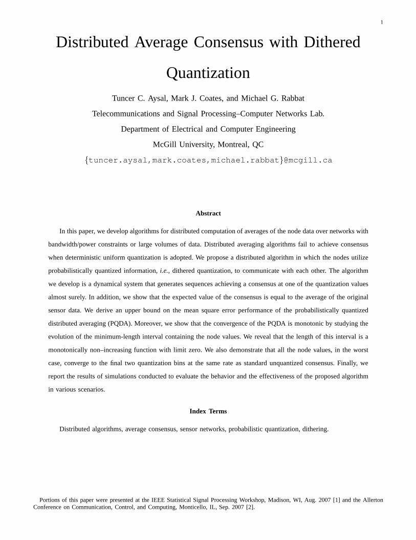
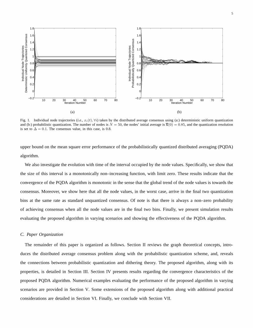
quantization does not lead to the desired result. Although the standard distributed averaging algorithm converges to
a fixed point when deterministic uniform quantization is used, it fails to converge to a consensus as illustrated in
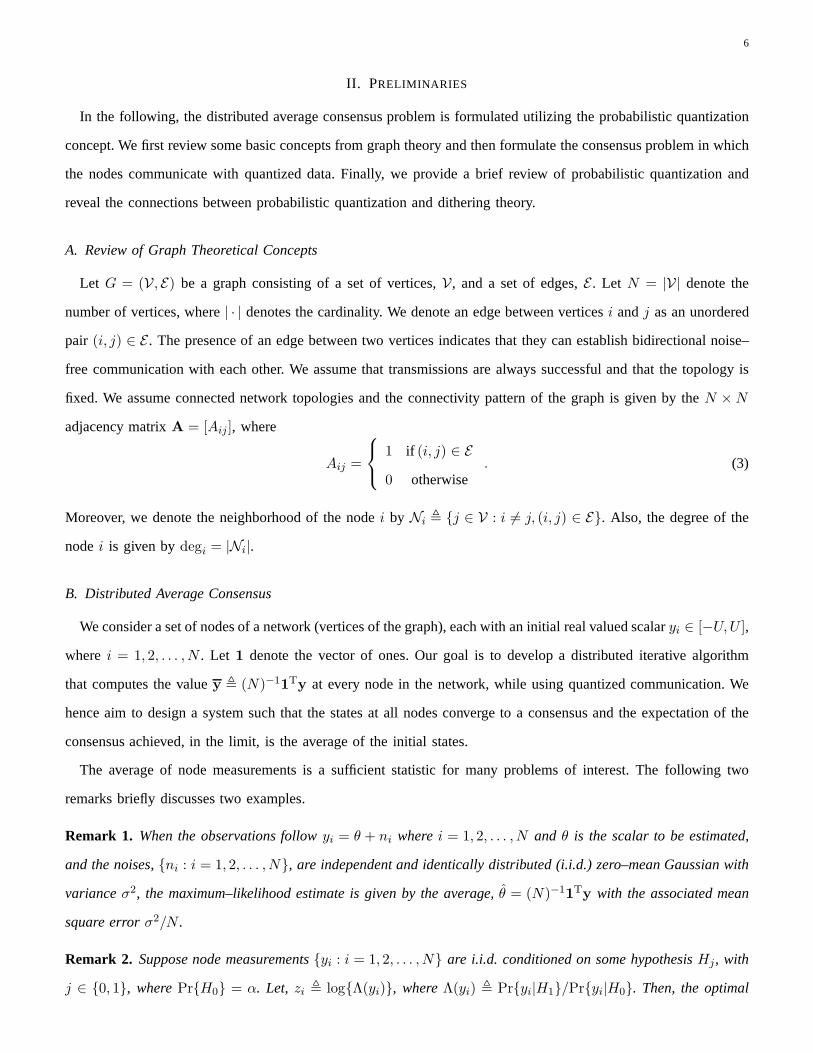
Fig. 1(a). Instead, we adopt the probabilistic quantization (PQ) scheme described in [4]. PQ has been shown to be
very effective for estimation with quantized data since thenoise introduced by PQ is zero-mean [4]. This makes
PQ suitable for average–based algorithms. As shown in Section II, the PQ algorithm is a form dithered quantization
method. Dithering has been widely recognized as a method to render the quantization noise independent of the
quantized data, reducing some artifacts created by deterministic quantization and there is a vast literature on the
topic, see [22] and reference therein.
In the scheme considered here, each node exchanges quantized state information with its neighbors in a simple
and bidirectional manner. This scheme does not involve routing messages in the network; instead, it diffuses
information across network by updating each node’s data with a weighted average of its neighbors’ quantized
ones. We do not burden the nodes with extensive computations, and we provide theoretical results,i.e., we show
here that the distributed average computation utilizing probabilistic consensus indeed achieves a consensus almost
surely (Fig. 1), and the consensus is one of the quantizationlevels. Furthermore, the expected value of the achieved
consensus is equal to the desired value,i.e., the average of the initial analog node measurements. We also give an
5
10 20 30 40 50 60 70 80−0.2
0
0.2
0.4
0.6
0.8
1
1.2
1.4
1.6
1.8
Iteration Number
Indi
vidu
al N
ode
Tra
ject
orie
s D
eter
min
istic
Uni
form
ly Q
uant
ized
Con
sens
us
(a)
10 20 30 40 50 60 70 80−0.2
0
0.2
0.4
0.6
0.8
1
1.2
1.4
1.6
1.8
Iteration Number
Indi
vidu
al N
ode
Tra
ject
orie
s P
roba
bilis
tical
ly Q
uant
ized
Con
sens
us
(b)
Fig. 1. Individual node trajectories (i.e., xi(t),∀i) taken by the distributed average consensus using (a:) deterministic uniform quantizationand (b:) probabilistic quantization. The number of nodes isN = 50, the nodes’ initial average isx(0) = 0.85, and the quantization resolutionis set to∆ = 0.1. The consensus value, in this case, is 0.8.
upper bound on the mean square error performance of the probabilistically quantized distributed averaging (PQDA)
algorithm.
We also investigate the evolution with time of the interval occupied by the node values. Specifically, we show that
the size of this interval is a monotonically non–increasingfunction, with limit zero. These results indicate that the
convergence of the PQDA algorithm is monotonic in the sense that the global trend of the node values is towards the
consensus. Moreover, we show here that all the node values, in the worst case, arrive in the final two quantization
bins at the same rate as standard unquantized consensus. Of note is that there is always a non–zero probability
of achieving consensus when all the node values are in the final two bins. Finally, we present simulation results
evaluating the proposed algorithm in varying scenarios andshowing the effectiveness of the PQDA algorithm.
C. Paper Organization
The remainder of this paper is organized as follows. SectionII reviews the graph theoretical concepts, intro-
duces the distributed average consensus problem along withthe probabilistic quantization scheme, and, reveals
the connections between probabilistic quantization and dithering theory. The proposed algorithm, along with its
properties, is detailed in Section III. Section IV presentsresults regarding the convergence characteristics of the
proposed PQDA algorithm. Numerical examples evaluating the performance of the proposed algorithm in varying
scenarios are provided in Section V. Some extensions of the proposed algorithm along with additional practical
considerations are detailed in Section VI. Finally, we conclude with Section VII.
6
II. PRELIMINARIES
In the following, the distributed average consensus problem is formulated utilizing the probabilistic quantization
concept. We first review some basic concepts from graph theory and then formulate the consensus problem in which
the nodes communicate with quantized data. Finally, we provide a brief review of probabilistic quantization and
reveal the connections between probabilistic quantization and dithering theory.
A. Review of Graph Theoretical Concepts
Let G = (V, E) be a graph consisting of a set of vertices,V, and a set of edges,E . Let N = |V| denote the
number of vertices, where| · | denotes the cardinality. We denote an edge between verticesi andj as an unordered
pair (i, j) ∈ E . The presence of an edge between two vertices indicates thatthey can establish bidirectional noise–
free communication with each other. We assume that transmissions are always successful and that the topology is
fixed. We assume connected network topologies and the connectivity pattern of the graph is given by theN × N
adjacency matrixA = [Aij ], where
Aij =
1 if (i, j) ∈ E
0 otherwise. (3)
Moreover, we denote the neighborhood of the nodei by Ni , {j ∈ V : i 6= j, (i, j) ∈ E}. Also, the degree of the
nodei is given bydegi = |Ni|.
B. Distributed Average Consensus
We consider a set of nodes of a network (vertices of the graph), each with an initial real valued scalaryi ∈ [−U,U ],
where i = 1, 2, . . . , N . Let 1 denote the vector of ones. Our goal is to develop a distributed iterative algorithm
that computes the valuey , (N)−11Ty at every node in the network, while using quantized communication. We
hence aim to design a system such that the states at all nodes converge to a consensus and the expectation of the
consensus achieved, in the limit, is the average of the initial states.
The average of node measurements is a sufficient statistic for many problems of interest. The following two
remarks briefly discusses two examples.
Remark 1. When the observations followyi = θ + ni wherei = 1, 2, . . . , N and θ is the scalar to be estimated,
and the noises,{ni : i = 1, 2, . . . , N}, are independent and identically distributed (i.i.d.) zero–mean Gaussian with
varianceσ2, the maximum–likelihood estimate is given by the average,θ̂ = (N)−11Ty with the associated mean
square errorσ2/N .
Remark 2. Suppose node measurements{yi : i = 1, 2, . . . , N} are i.i.d. conditioned on some hypothesisHj, with
j ∈ {0, 1}, wherePr{H0} = α. Let, zi , log{Λ(yi)}, whereΛ(yi) , Pr{yi|H1}/Pr{yi|H0}. Then, the optimal
7
decision is to perform the following detection rule:z ≷H1
H0
α/(1 − α) wherez , (N)−11Tz.
C. Probabilistic Quantization and Dithering
In the following, we present a brief review of the quantization scheme adopted in this paper. Suppose that
the scalar valuexi ∈ R is bounded to a finite interval[−U,U ]. Furthermore, suppose that we wish to obtain a
quantized messageqi with length l bits, wherel is application dependent. We therefore haveL = 2l quantization
points given by the setτ = {τ1, τ2, . . . , τL} whereτ1 = −U and τL = U . The points are uniformly spaced such
that ∆ = τj+1 − τj for j ∈ {1, 2, . . . , L − 1}. It follows that ∆ = 2U/(2l − 1). Now supposexi ∈ [τj , τj+1) and
let qi , Q(xi) whereQ(·) denotes the PQ operation. Thenxi is quantized in a probabilistic manner:
Pr{qi = τj+1} = r, and, Pr{qi = τj} = 1 − r (4)
wherer = (xi−τj)/∆. Of note is that when the variable to quantize is exactly equal to a quantization centroid, there
is zero probability of choosing another centroid. The following lemma, adopted from [4], discusses two important
properties of PQ.
Lemma 1. [4] Supposexi ∈ [τj, τj+1) and letqi be anl–bit quantization ofxi ∈ [−U,U ]. The messageqi is an
unbiased representation ofxi, i.e.,
E{qi} = xi, and, E{(qi − xi)2} ≤ U2
(2l − 1)2≡ ∆2
4. (5)
As noted in the following lemma, a careful observation showsthat probabilistic quantization is equivalent to a
“dithered quantization” method.
Lemma 2. Supposexi ∈ [τj , τj+1) and let qi , Q(xi). Probabilistic quantization is equivalent to the following
dithered quantization scheme:
qi = minj
|τj − (xi + u)| (6)
whereu is a uniform random variable with support on[−∆/2,∆/2].
Proof: Without loss of generality, suppose|τj − xi| < |τj+1 − xi|. Moreover, suppose we are utilizing a
deterministic uniform quantizer. Then,
Pr{qi = τj} = Pr
{
τj −∆
2≤ xi + u ≤ τj −
∆
2
}
(7)
= Pr
{
u ≤ τj +∆
2− xi
}
(8)
=τj+1 − xi
∆. (9)
8
Note that the last line is equivalent to1 − r, so the proof is complete.
Thus, before we perform any quantization, we add uniform random variableu with support defined on[−∆/2,∆/2]
and we form x′i = u + xi. Now, performing standard deterministic uniform quantization, i.e., letting qi =
minj |τj−x′i|, yields quantized values,qi’s that are statistically identical to the ones of the probabilistic quantization.
Thus, probabilistic quantization is a form of dithering where one, before performing standard deterministic uniform
quantization, adds a uniform random variable with support equal to the quantization bin size. This is a substractively
dithered system [22]. It has been shown by Schuchman that thesubstractive dithering process utilizing uniform
random variable with support on[−∆/2,∆/2] yields error signal values that are statistically independent from each
other and the input [23].
III. D ISTRIBUTED AVERAGE CONSENSUS WITHPROBABILISTICALLY QUANTIZED COMMUNICATION
In the following, we propose a quantized distributed average consensus algorithm and incorporate PQ into
the consensus framework for networks. Furthermore, we analyze the effect of PQ on the consensus algorithm.
Specifically, we present theorems revealing the limiting consensus, expectation and mean square error of the
proposed PQDA algorithm.
At t = 0 (after all sensors have taken the measurement), each node initializes its state asxi(0) = yi, i.e.,
x(0) = y wherex(0) denotes the initial states at the nodes. It then quantizes its state to generateqi(0) = Q(xi(0)).
At each following step, each node updates its state with a linear combination of its own quantized state and the
quantized states at its neighbors
xi(t + 1) = Wiiqi(t) +∑
j∈Ni
Wijqj(t) (10)
for i = 1, 2, . . . , N , whereqj(t) = Q(xj(t)), andt denotes the time step. Also,Wij is the weight onxj(t) at node
i. Moreover, settingWij = 0 wheneverΦij = 0, the distributed iterative process reduces to the following recursion
x(t + 1) = Wq(t) (11)
whereq(t) denotes the quantized state vector, followed by
q(t + 1) = Q(x(t + 1)). (12)
The PQDA algorithm hence refers to the iterative algorithm defined by (11) and (12). In the sequel, we assume
thatW, the weight matrix, is symmetric, non-negative and satisfies the conditions required for asymptotic average
consensus without quantization [19]:
W1 = 1, 1TW = 1T, and,ρ(W − J) < 1, (13)
9
whereρ(U) denotes the spectral radius of a matrixU (i.e., the largest eigenvalue ofU in absolute value), and
J , (N)−111T, whereJx projectsx onto theN–dimensional “diagonal” subspace (i.e., the set of vectors inRN
corresponding to a strict consensus). Weight matrices satisfying the required convergence conditions are easy to
find if the underlying graph is connected and non–bipartite,e.g., Maximum–degree and Metropolis weights [19].
The following theorem considers the convergence of the probabilistically quantized distributed average compu-
tation.
Theorem 1. The probabilistically quantized distributed iterative process achieves a consensus, almost surely,i.e.,
Pr{
limt→∞
x(t) = c1}
= 1 (14)
wherec ∈ τ .
Proof: Without loss of generality, we focus on integer quantization in the range[1,m]. DefineM as the
discrete Markov chain with initial stateq(0) and transition matrix defined by the combination of the deterministic
transformationx(t + 1) = Wq(t) and the probabilistic quantizerq(t + 1) ∼ Pr{q(t + 1)|x(t + 1)}.
Let S0 be the set of quantization points that can be represented in the formq1 for some integerq and denote by
Sk the set of quantization points with Manhattan distancek from S0. Moreover, letC(q) be the open hypercube
centered atq and defined as(q1 − 1, q1 + 1) × (q2 − 1, q2 + 1) × ...× (qN − 1, qN + 1). Hereqk denotes thek–th
coefficient ofq. Note that any point inC(q) has a non-zero probability of being quantized toq. Let
Ak =⋃
q∈Sk
C(q). (15)
The consensus operator has the important property that|Wq−µ(Wq)| < |q−µ(q)| for |q−µ(q)| > 0, where
µ(·) denotes the projection of its argument onto the1–vector. Moreover,cW1 = c1. The latter property implies
thatq ∈ S0 is an absorbing state, sinceQ(x(t + 1)) = Q(Wq(t)) = Q(q(t)) = q(t). The former property implies
that there are no other absorbing states, sincex(t + 1) cannot equalq(t) (it must be closer to the1–vector). This
implies, from the properties of the quantizerQ, that there is a non-zero probability thatq(t + 1) 6= q(t).
In order to prove thatM is an absorbing Markov chain, it remains to show that it is possible to reach an
absorbing state from any other state. We prove this by induction, demonstrating first that
Pr{q(t + 1) ∈ S0|q(t) ∈ S1} > 0 (16)
and subsequently that
Pr{q(t + 1) ∈k−1⋃
i=0
Si|q(t) ∈ Sk} > 0. (17)
10
Define the open setVk as
Vk ={
x : |x − µ(x)| < k√
N − 1/√
N}
. (18)
To commence, observe thatV1 ⊂ A0. The distance|q−µ(q)| =√
N − 1/√
N for q ∈ S1. Hence, ifq(t) ∈ S1,
x(t + 1) = Wq(t) ∈ V1 ∈ A0 andPr{q(t + 1) ∈ S0} > 0. Similarly, the set
Vk ⊂k−1⋃
i=0
Ai (19)
is contained in the union of the firstk hypercubes,Ai, i = 0, 1, . . . , k − 1. The maximum distance|q − µ(q)| for
any pointq ∈ Sk is k√
N − 1/√
N . This implies that
x(t + 1) = Wq(t) ∈ Vk ∈k−1⋃
i=0
Ai. (20)
There is thus somei < k and someq ∈ Si such thatPr{Q(x(t + 1)) = q} > 0. This argument implies that
for any starting stateq(0) such thatq(0) ∈ Sk for somek, there exists a sequence of transitions with non–zero
probability whose application results in absorption.
The theorem reveals that the probabilistically quantized distributed process indeed achieves a strict consensus at
one of the quantization values. It is of interest to note thatthe stationary points of the PQDA algorithm are in the
form of c1 wherec ∈ τ . We, hence, construct an absorbing Markov chain where the absorbing states are given
by the stationarity points and show that for any starting state, there exists a sequence of transitions with non–zero
probability whose application results in absorption. The following theorem discusses the expectation of the limiting
random vector,i.e., the expected value ofx(t) as t tends to infinity.
Theorem 2. The expectation of the limiting random vector is given by
E
{
limt→∞
x(t)}
= (N)−111Tx(0). (21)
Proof: Note that||x(t)|| ≤√
NU , for t ≥ 0, and,{xi(t) : i = 1, 2, . . . , N} is bounded for allt. Moreover,
from Theorem 1, we know that the random vector sequencex(t) converges in the limit,i.e., limt→∞ x(t) = c1 for
somec ∈ τ . Thus, by the Lebesgue dominated convergence theorem [24],we have
E
{
limt→∞
x(t)}
= limt→∞
E{x(t)}. (22)
In the following, we derivelimt→∞ E{x(t)} and utilize the above relationship to arrive at the desired result.
In terms of quantization noisev(t), we can writeq(t) = x(t) + v(t). The distributed iterative process reduces

11
to the following recursionx(t + 1) = Wx(t) + Wv(t). Repeatedly utilizing the state recursion gives
x(t) = Wtx(0) +
t−1∑
j=0
Wt−jv(j). (23)
Taking the statistical expectation ofx(t) as t → ∞ and noting that the only random variables arev(j) for
j = 0, 1, . . . , t − 1, yields
limt→∞
E{x(t)} = limt→∞
Wtx(0) +
t−1∑
j=0
Wt−jE{v(j)} (24)
= limt→∞
Wtx(0) (25)
since E{v(j)} = 0 for j = 0, 1, . . . , t − 1; a corollary of Lemma 1. Furthermore, noting thatlimt→∞ Wt =
(N)−111T gives
limt→∞
E{x(t)} = (N)−111Tx(0). (26)
Recalling (22) gives the desired result.
This result indicates that the expectation of the limiting random vector is indeed equal to the initial analog node
measurements’ average. Furthermore, this theorem, combined with the previous one, indicates that the consensus
value,c, is a discrete random variable with support defined byτ , and whose expectation is equal to the average of
the initial states.
After establishing that the consensus value is a random variable with the desired expectation in the limit, the
next natural quantity of interest is the limiting mean squared error,i.e., the limiting average squared distance of the
consensus random variable from the desired initial states’average value. The following theorem, thus, considers
the expectation of the error norm of probabilistically quantized consensus ast andN tend to infinity.
Theorem 3. Let us definex(0) , Jx(0). The expectation of the error norm of the probabilisticallyquantized
distributed average consensus is asymptotically bounded by
limt→∞
limN→∞
(√
N)−1E{||q(t) − x(0)||} ≤ ∆
2
1
1 − ρ(W − J)(27)
whereρ(·) denotes the spectral radius of its argument.
Proof: See Appendix A.
The proof exploits averaging characteristics ofW, properties of norm operators, and uses a Law of Large
Numbers argument to bound the error contributed by quantization noise.
Note that the upper bound decreases with decreasing spectral radius of(W−J), where a smaller (larger)ρ(W−J)
can be, in a loose manner, interpreted as better (worse) “averaging ability” of the weight matrix. Furthermore, as
12
expected, the upper bound on the error norm increases with decreasing quantization resolution (i.e., increasing∆).
IV. CONVERGENCECHARACTERISTICS OFPROBABILISTICALLY QUANTIZED DISTRIBUTED AVERAGE
CONSENSUS
The convergence characteristics of the PQDA are essential for further understanding of the algorithm. In the
following, we consider the evolution of the intervals occupied by the quantized and unquantized state values.
Interestingly, we reveal that the length of the smallest interval containing all of the quantized state values, (i.e.,
the range of the quantized state values) is non–increasing with a limit of zero as the time step tends to infinity.
Moreover, we show that size of the minimum length interval, with boundaries constrained to the quantization points,
that contains all of the unquantized node state values, is also non–increasing. This also has limit zero as the time
step tends to infinity.
Let us denote the smallest and largest order statistics of any vectoru ∈ RN as u(1) , mini{ui} and u(N) ,
maxi{ui}, respectively. Furthermore, letI[x(t)] denote the interval of the node state values at timet, i.e., the
interval in which{xi(t) : i = 1, 2, . . . , N} values lie,
I[x(t)] , [x(1)(t), x(N)(t)] (28)
and I[q(t)] denote the domain of the quantized node state values at timet, i.e.,
I[q(t)] , [q(1)(t), q(N)(t)]. (29)
Moreover, let
τL(t) , maxj
{τj : xi(t) ≥ τj,∀i} (30)
and
τU (t) , minj
{τj : xi(t) ≤ τj,∀i} (31)
along with I[τ(t)] , [τL(t), τU (t)].
The following theorem discusses the evolution of the interval of the quantized node state values, and the minimum
range quantization bin that encloses the node state values.The theorem reveals that both intervals are non–expanding.
Theorem 4. For somet ≥ 0, suppose thatqi(t) ∈ I[q(t)], and,xi(t) ∈ I[x(t)], for i = 1, 2, . . . , N . By construction
I[x(t)] ⊆ I[τ(t)]. (32)
Then, fork ≥ 1, the followings hold:

13
(i) The interval of the quantized state vector is non–expanding, i.e.,
I[q(t + k)] ⊆ I[q(t)]. (33)
(ii) The minimum length interval with boundaries defined by quantization points that encloses the state vector
values is non–expanding,i.e.,
I[x(t + k)] ⊆ I[τ(t + k)] ⊆ I[τ(t)]. (34)
Proof: Consider (i) first. Suppose thatqi(t) ∈ I[q(t)], for i = 1, 2, . . . , N , and recall that the state recursion
follows asx(t+1) = Wq(t). Let wi denote the row vector formed as thei–th row of the weight matrixW. Now,
we can write the node specific update equation as
xi(t + 1) = wiq(t). (35)
Note thatxi(t + 1) is a linear combination of quantized local node values andwij ≥ 0 for j = 1, 2, . . . , N , where
wij denotes thej–th entry ofwi. Moreover,wi1 = 1, sinceW1 = 1. Thus,xi(t + 1) is a convex combination of
the quantized node state values and its own quantized state.The node state valuexi(t + 1) is then in the convex
hull of quantized state values{qi(t) : i = 1, 2, . . . , N}. The convex hull of the quantized state values at timet is
given by I[q(t)], indicating that
xi(t + 1) ∈ I[q(t)] (36)
for i = 1, 2, . . . , N , and subsequently,
I[x(t + 1)] ⊆ I[q(t)]. (37)
Hence, we see that
q(N)(t + 1) = Q(xi(t + 1)) ≤ q(N)(t) (38)
for somei ∈ {1, 2, . . . , N} and
q(1)(t + 1) = Q(xj(t + 1)) ≥ q(1)(t) (39)
for somej ∈ {1, 2, . . . , N} andj 6= i. It follows that
I[q(t + 1)] ⊆ I[q(t)]. (40)
Repeatedly utilizing the above steps completes the proof.
Now consider (ii). Suppose thatxi(t) ∈ I[x(t)] for i = 1, 2, . . . , N . Then, by construction,I[x(t)] ⊆ I[τ(t)].

14
Furthermore, since
τL(t) ≤ q(1)(t) (41)
and
τU (t) ≥ q(N)(t) (42)
it follows that
qi(t) = Q(xi(t)) ∈ I[q(t)] ⊆ I[τ(t)] (43)
for i = 1, 2, . . . , N . The convex combination property, similar to the previous case, indicates that,xi(t+1) ∈ I[q(t)]
for i = 1, 2, . . . , N , and subsequently,I[x(t + 1)] ⊆ I[q(t)]. Moreover, since,I[q(t)] ⊆ I[τ(t)], it follows that
I[x(t + 1)] ⊆ I[τ(t)]. (44)
Finally combining all the results indicating that
I[x(t + 1)] ⊆ I[q(t + 1)] ⊆ I[τ(t + 1)] ⊆ I[τ(t)] (45)
and repeatedly utilizing the above steps completes the proof.
The proof of this theorem indicates that each iteration is indeed a convex combination of the previous set of
quantized node state values, and uses of the properties of convex functions to arrive at the stated results.
Let us definerq(t) as the Lebesgue measure of the domain of the quantized state vector at time stept, i.e., the
range ofq(t) ∈ RN ,
rq(t) , q(N)(t) − q(1)(t) (46)
whererq(t) ∈ {0,∆, . . . , (L − 1)∆}. Similar to the quantized state vector case, we definerτ (t) , τU(t) − τL(t)
as the length of the intervalI[τ(t)].
The following corollary (the proof of which is omitted sinceit follows directly from Theorem 1 and Theorem 4),
compiled from Theorem 1 and Theorem 4, discusses propertiesof interest ofrq(t) andrτ (t).
Corollary 1. The functionsrq(t) and rτ (t), with initial conditionsrq(0) ≥ 0 and rτ (0) ≥ 0, tend to zero ast
tends to infinity,i.e.,
limt→∞
rq(t) = 0 (47)
and
limt→∞
rτ (t) = 0. (48)
15
Moreover,rq(t) and rτ (t) are monotonically non–increasing functions.
The presented theorem and corollary indicate that the convergence of the PQDA is monotonic in the sense that
the global trend of both the quantized and unquantized node state values is towards the consensus and that the
minimum-length intervals containing all values do not expand, and in fact, converge to zero-length monotonically.
The following theorem investigates the rate of convergenceof the PQDA to a state where there is a first time
non–zero probability of converging to the consensus (all values are contained within two quantization bins).
Theorem 5. Let rq(t) , q(N)(t) − q(1)(t) and rx(t) , x(N)(t) − x(1)(t) denote the range of the quantized and
unquantized node state values at time stept, with the initial valuesrq(0) and rx(0), respectively. Then,
E{rq(t)} ≤√
N − 1
Nρt(W − J)rx(0) + 2∆ (49)
whereρ(·) denotes the spectral radius of its argument.
Proof: See Appendix B.
In the appendix, we compile an upper and lower bound on the largest and smallest order statistics of the quantized
node state vector using results from [25]. Then, the task reduces to deriving a bound on the convergence rate of the
normed difference of any rowi andj with time, and combining this bound with the bounds on the order statistics
gives the desired result.
Theorem 5 reveals that the PQDA converges to the final two binswith the same rate as standard consensus.
Theorem 5 also relates the convergence of the quantized nodestate values range to the range of initial node
measurements.
After all the node state values are in the final two bins, thereis always a non–zero probability to immediately
converge to consensus. Note that, in the absence of knowledge of the norm of the initial node states or the initial
state range, the bound given above reduces to
E{rq(t)} ≤ 2
√
N − 1
Nρt(W − J)U + 2∆ (50)
where we used the facts thatmaxi{xi(0)} ≤ U andmini{xi(0)} ≥ −U .
To understand the convergence of the PQDA algorithm after all the quantized states converged to the final two
bins, first, let us discuss the behavior of the PQDA algorithmin the final bin,i.e., maxi{qi(t)}−mini{qi(t)} = ∆.
Supposexi(t) ∈ [τj, τj+1], for somej. In this case, all the nodes state values need to be quantizedto τj or τj+1
to achieve a consensus at time stept. Hence, the effect of the weight matrix on the convergence rate significantly
decreases and the convergence rate is mainly dominated by the probabilistic quantization. Moreover, we hence
believe that the time interval, where all the node state values are inτj andτj + 2∆, is a transition period between
16
the dominating effect of the weight matrix,i.e., the spectral radius ofW − J, and the dominating effect of
probabilistic quantization. Obtaining analytical expressions of convergence rate for these transition and final bin
regions appears to be a challenging task. Although our current research efforts focus on this challenge, we assess
the convergence performance of the PQDA algorithm with extensive simulations in the following section.
V. NUMERICAL EXAMPLES
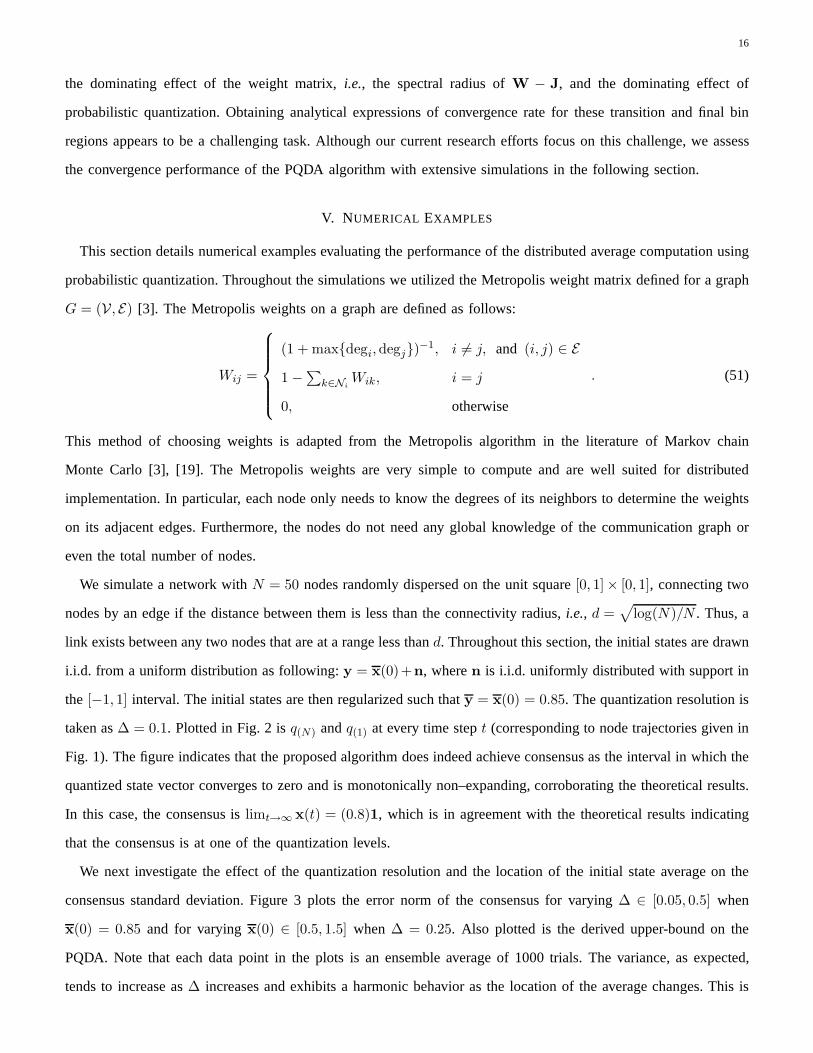
This section details numerical examples evaluating the performance of the distributed average computation using
probabilistic quantization. Throughout the simulations we utilized the Metropolis weight matrix defined for a graph
G = (V, E) [3]. The Metropolis weights on a graph are defined as follows:
Wij =
(1 + max{degi,degj})−1, i 6= j, and (i, j) ∈ E
1 −∑k∈NiWik, i = j
0, otherwise
. (51)
This method of choosing weights is adapted from the Metropolis algorithm in the literature of Markov chain
Monte Carlo [3], [19]. The Metropolis weights are very simple to compute and are well suited for distributed
implementation. In particular, each node only needs to knowthe degrees of its neighbors to determine the weights
on its adjacent edges. Furthermore, the nodes do not need anyglobal knowledge of the communication graph or
even the total number of nodes.
We simulate a network withN = 50 nodes randomly dispersed on the unit square[0, 1]× [0, 1], connecting two
nodes by an edge if the distance between them is less than the connectivity radius,i.e., d =√
log(N)/N . Thus, a
link exists between any two nodes that are at a range less thand. Throughout this section, the initial states are drawn
i.i.d. from a uniform distribution as following:y = x(0)+n, wheren is i.i.d. uniformly distributed with support in
the [−1, 1] interval. The initial states are then regularized such thaty = x(0) = 0.85. The quantization resolution is
taken as∆ = 0.1. Plotted in Fig. 2 isq(N) andq(1) at every time stept (corresponding to node trajectories given in
Fig. 1). The figure indicates that the proposed algorithm does indeed achieve consensus as the interval in which the
quantized state vector converges to zero and is monotonically non–expanding, corroborating the theoretical results.
In this case, the consensus islimt→∞ x(t) = (0.8)1, which is in agreement with the theoretical results indicating
that the consensus is at one of the quantization levels.
We next investigate the effect of the quantization resolution and the location of the initial state average on the
consensus standard deviation. Figure 3 plots the error normof the consensus for varying∆ ∈ [0.05, 0.5] when
x(0) = 0.85 and for varyingx(0) ∈ [0.5, 1.5] when ∆ = 0.25. Also plotted is the derived upper-bound on the
PQDA. Note that each data point in the plots is an ensemble average of 1000 trials. The variance, as expected,
tends to increase as∆ increases and exhibits a harmonic behavior as the location of the average changes. This is

17
10 20 30 40 50 60 70 80−0.2
0
0.2
0.4
0.6
0.8
1
1.2
1.4
1.6
1.8
Iteration Number
Qua
ntiz
ed S
tate
Vec
tor
Inte
rval
Fig. 2. The plotted are is the interval in which the quantizedstate vector is. The number of nodes isN = 50, the nodes’ initial average isx(0) = 0.85, and the quantization resolution is set to∆ = 0.1.
0.05 0.1 0.15 0.2 0.25 0.3 0.35 0.4 0.4510
−2
10−1
100
Quantization Resolution
Con
sens
us S
tand
ard
Dev
iatio
n
Simulated DeviationTheoretical Bound
(a)
0.5 0.75 1.0 1.25 1.5
0.09
0.1
0.11
0.12
0.13
0.14
Average of Initial States
Con
sens
us S
tand
ard
Dev
iatio
n
(b)
Fig. 3. The error norm of the consensus with respect to (a) thequantization resolution,i.e., ∆ ∈ [0.05, 0.5] with x(0) = 0.85 and (b) theinitial state average with∆ = 0.25. The network parameter are:N = 50 andd =
√
log(N)/N .
due to the effect induced by the distance of the average to thequantization levels.
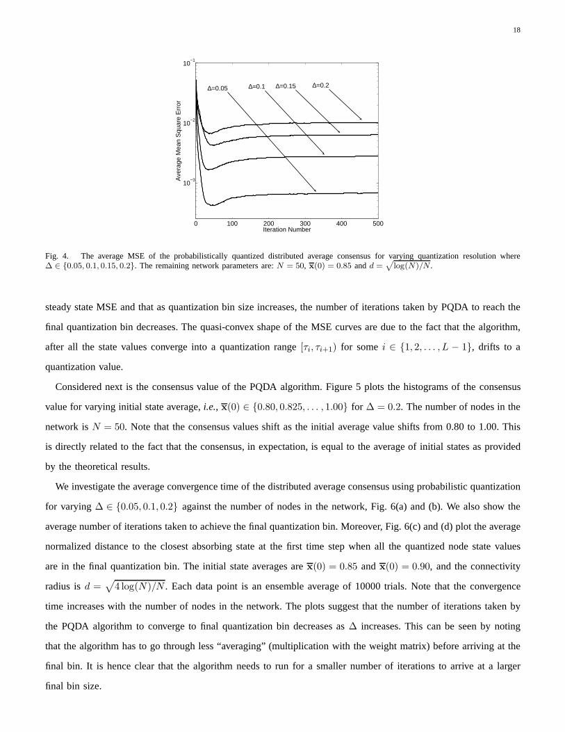
Figure 4 shows the behavior of the average mean square error (MSE) per iteration defined as:
MSE(t) =1
N
N∑
i=1
(xi(t) − x(0))2 (52)
for ∆ ∈ {0.05, 0.1, 0.15, 0.2}. In other words,MSE(t) is the average mean squared distance of the states at iteration
t from the initial mean. Each curve is an ensemble average of 1000 experiments and the network parameters are:
N = 50, x(0) = 0.85 and d =√
log(N)/N . The plots suggest that smaller quantization bins yield a smaller
18
0 100 200 300 400 500
10−3
10−2
10−1
Iteration Number
Ave
rage
Mea
n S
quar
e E
rror
∆=0.2∆=0.15∆=0.1∆=0.05
Fig. 4. The average MSE of the probabilistically quantized distributed average consensus for varying quantization resolution where∆ ∈ {0.05, 0.1, 0.15, 0.2}. The remaining network parameters are:N = 50, x(0) = 0.85 andd =
√
log(N)/N .
steady state MSE and that as quantization bin size increases, the number of iterations taken by PQDA to reach the
final quantization bin decreases. The quasi-convex shape ofthe MSE curves are due to the fact that the algorithm,
after all the state values converge into a quantization range [τi, τi+1) for somei ∈ {1, 2, . . . , L − 1}, drifts to a
quantization value.
Considered next is the consensus value of the PQDA algorithm. Figure 5 plots the histograms of the consensus
value for varying initial state average,i.e., x(0) ∈ {0.80, 0.825, . . . , 1.00} for ∆ = 0.2. The number of nodes in the
network isN = 50. Note that the consensus values shift as the initial averagevalue shifts from 0.80 to 1.00. This
is directly related to the fact that the consensus, in expectation, is equal to the average of initial states as provided
by the theoretical results.
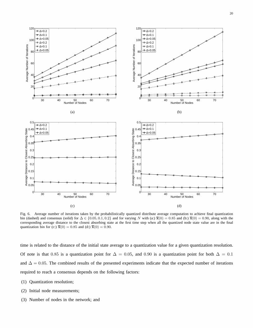
We investigate the average convergence time of the distributed average consensus using probabilistic quantization
for varying ∆ ∈ {0.05, 0.1, 0.2} against the number of nodes in the network, Fig. 6(a) and (b).We also show the
average number of iterations taken to achieve the final quantization bin. Moreover, Fig. 6(c) and (d) plot the average
normalized distance to the closest absorbing state at the first time step when all the quantized node state values
are in the final quantization bin. The initial state averagesarex(0) = 0.85 andx(0) = 0.90, and the connectivity
radius isd =√
4 log(N)/N . Each data point is an ensemble average of 10000 trials. Notethat the convergence
time increases with the number of nodes in the network. The plots suggest that the number of iterations taken by
the PQDA algorithm to converge to final quantization bin decreases as∆ increases. This can be seen by noting
that the algorithm has to go through less “averaging” (multiplication with the weight matrix) before arriving at the
final bin. It is hence clear that the algorithm needs to run fora smaller number of iterations to arrive at a larger
final bin size.

19
0.4 0.6 0.8 1 1.2 1.40
0.2
0.4
0.6
0.8
0.4 0.6 0.8 1 1.2 1.40
0.2
0.4
0.6
0.8
0.4 0.6 0.8 1 1.2 1.40
0.2
0.4
0.6
0.8
0.4 0.6 0.8 1 1.2 1.40
0.2
0.4
0.6
0.8
Nor
mal
ized
Num
ber
of O
ccur
ence
0.4 0.6 0.8 1 1.2 1.40
0.2
0.4
0.6
0.8
0.4 0.6 0.8 1 1.2 1.40
0.2
0.4
0.6
0.8
0.4 0.6 0.8 1 1.2 1.40
0.2
0.4
0.6
0.8
0.4 0.6 0.8 1 1.2 1.40
0.2
0.4
0.6
0.8
Value0.4 0.6 0.8 1 1.2 1.4
0
0.2
0.4
0.6
0.8
x(0)=0.8 x(0)=0.825 x(0)=0.85
x(0)=0.875 x(0)=0.9 x(0)=0.925
x(0)=0.95 x(0)=0.975 x(0)=1.0
Fig. 5. Histograms of the consensus value achieved by the probabilistically quantized consensus for varying initial state average wherex(0) ∈ {0.80, 0.825, . . . , 1.00} and∆ = 0.2. The number of nodes in the network isN = 50.
On the other hand, as discussed in more detail below, the expected number of iterations taken to achieve consensus
is dominated by the number of iterations taken to converge toan absorbing state after all the node values are in
the final bin. The probabilistic quantization is the dominant effect in the final bin. The time taken to converge to
an absorbing state is heavily dependent on the distance to that absorbing state at the first time step when all values
enter the final bin. This distance is affected by two factors.First, if more averaging operations occur prior to the
entry step, then there is more uniformity in the values, decreasing the distance. Second, if the initial data average
is close to a quantization value, then, on average, the entrypoint will be closer to an absorbing state (note that
E{1Tq(t)} = 1Tx(0)). These observations explain the results of Fig. 6. Note that the convergence time order for
x(0) = 0.85 andx(0) = 0.90 cases flip for∆ = 0.2 and∆ = 0.1. That is due to the fact that the average distance
to an absorbing when, at the first time step, all the node values enter the final bin is smaller forx(0) = 0.85 when
∆ = 0.2 compared to∆ = 0.1, and is smaller forx(0) = 0.90 when∆ = 0.1 compared to∆ = 0.2. Moreover,
note that∆ = 0.05 yields the smallest distance to an absorbing state for both initial conditions. Although, it takes
more iterations to converge to final bin, in both cases, PQDA algorithm with ∆ = 0.05 yields the smallest average
distance to an absorbing state when all the node values enterto the final bin for the first time step, hence, the
smallest average number of iterations to achieve the consensus.
We consider next the effect of the connectivity radius on theaverage number of iterations taken to achieve
the consensus. Figure 7 depicts the average number of iterations to achieve the consensus for the cases where the
initial state average isx(0) = 0.85 andx(0) = 0.90. As expected, the average number of iterations taken to achieve
consensus decreases with increasing connectivity radius.This is related to the fact that higher connectivity radius,
implies a lower second largest eigenvalue for the weight matrix. Moreover, as in the previous case, the convergence
20
30 40 50 60 700
20
40
60
80
100
120
Number of Nodes
Ave
rage
Num
ber
of It
erat
ions
∆=0.2∆=0.1∆=0.05∆=0.2∆=0.1∆=0.05
(a)
30 40 50 60 700
20
40
60
80
100
120
Number of Nodes
Ave
rage
Num
ber
of It
erat
ions
∆=0.2∆=0.1∆=0.05∆=0.2∆=0.1∆=0.05
(b)
30 40 50 60 700
0.05
0.1
0.15
0.2
0.25
0.3
0.35
0.4
0.45
0.5
Number of Nodes
Ave
rage
Dis
tanc
e to
Clo
sest
Abs
orbi
ng S
tate
∆=0.2∆=0.1∆=0.05
(c)
30 40 50 60 700
0.05
0.1
0.15
0.2
0.25
0.3
0.35
0.4
0.45
0.5
Number of Nodes
Ave
rage
Dis
tanc
e to
Clo
sest
Abs
orbi
ng S
tate
∆=0.2∆=0.1∆=0.05
(d)
Fig. 6. Average number of iterations taken by the probabilistically quantized distribute average computation to achieve final quantizationbin (dashed) and consensus (solid) for∆ ∈ {0.05, 0.1, 0.2} and for varyingN with (a:) x(0) = 0.85 and (b:)x(0) = 0.90, along with thecorresponding average distance to the closest absorbing state at the first time step when all the quantized node state value are in the finalquantization bin for (c:)x(0) = 0.85 and (d:)x(0) = 0.90.
time is related to the distance of the initial state average to a quantization value for a given quantization resolution.
Of note is that0.85 is a quantization point for∆ = 0.05, and 0.90 is a quantization point for both∆ = 0.1
and∆ = 0.05. The combined results of the presented experiments indicate that the expected number of iterations
required to reach a consensus depends on the following factors:
(1) Quantization resolution;
(2) Initial node measurements;
(3) Number of nodes in the network; and

21
1 1.5 2 2.5 3 3.5 4 4.5 50
20
40
60
80
100
120
Connectivity Radius Factor
Ave
rage
Num
ber
of It
erat
ions
for
Con
verg
ence
∆=0.2∆=0.1∆=0.05
(a)
1 1.5 2 2.5 3 3.5 4 4.5 50
20
40
60
80
100
120
Connectivity Radius Factor
Ave
rage
Num
ber
of It
erat
ions
for
Con
verg
ence
∆=0.2∆=0.1∆=0.05
(b)
Fig. 7. Average number of iterations taken by the probabilistically quantized distribute average computation for∆ ∈ {0.05, 0.1, 0.2} with(a:) x(0) = 0.85 and (b:)x(0) = 0.90. The number of nodes in the network isN = 50. Connectivity radius factor is defined as themodulating constantk, in the expression for the connectivity radiusd = k
√
log(N)/N .
(4) Connectivity radius.
Note that (1), (3) and (4) are system design choices, affected by energy budgets and bandwidth constraints, but (2)
is data-dependent. This implies that the quantization resolution, given the bandwidth and power constraints of the
application, should be chosen to minimize the expected (or worst-case) convergence time over the range of possible
initial averages.
VI. FURTHER CONSIDERATIONS
The analysis presented in this paper makes two main simplifying assumptions: 1) the network topology does
not change over time, and 2) communication between neighboring nodes is always successful. The simplifying
assumptions essentially allow us to focus on the case where the weight matrix,W, does not change with time.
However, time-varying topologies and unreliable communications are important practical issues which have been
addressed for un-quantized consensus algorithms (see,e.g., [3], [26], [27]). SinceW has the same support as
the adjacency matrix of the underlying communication graph, when the topology changes with time, the averaging
weights must also vary. Likewise, an unsuccessful transmission between two nodes is equivalent to the link between
those nodes vanishing for one iteration. In either case, we can now think ofW(t) as random process. Typical results
for this scenario roughly state that average consensus is still accomplished when the weight matrix varies with time,
so long as the expected weight matrix,E[W(t)], is connected. This condition ensures that there is always non-zero
probability that information will diffuse throughout the network. We expect that the same techniques employed
in [3], [26], [27] can be used to show convergence of our average consensus with probabilistic quantization with
22
time-varyingW.
In this paper we also restricted ourselves to the scenario where the quantization step size∆ remains fixed over all
time. Recall that when the algorithm has converged to a consensus, allqi(t) are at the same quantization point, so
‖q(t)−Jq(t)‖ = 0. Letting D(t) , ‖q(t)−Jq(t)‖ denote Euclidean distance to convergence, we know that when
the algorithm is far from converging (i.e., D(t) large), quantization errors have less of an effect on convergence of
the algorithm. This is because the averaging effects ofW are multiplicative and thus have a stronger influence when
D(t) is large, whereas the quantization error is bounded by a constant which only depends on∆ and not onD(t).
WhenD(t) is of the same order as the quantization noise variance, quantization essentially wipes away the effects
of averaging and hampers the time to convergence. A natural extension of the algorithm proposed in this paper
involves shrinking the quantization step size,∆, over time,e.g., setting∆new = ∆old/2 onceD(t) is established
to be below the threshold where quantization effects outweigh averaging. We expect that this modification should
improve the rate at whichD(t) tends to zero without affecting statistical properties of the limiting consensus values
(i.e., unbiased w.r.t. tox(0), and no increase in the limiting variance). Solidifying this procedure is a topic of
current investigation.
VII. C ONCLUDING REMARKS
We have described probabilistically quantized distributed averaging (PQDA), a framework for distributed com-
putation of averages of the node data over networks with bandwidth/power constraints or large volumes of data.
The proposed method unites the distributed average consensus algorithm and probabilistic quantization, which is
a form of “dithered quantization”. The proposed PQDA algorithm achieves a consensus, and the consensus is a
discrete random variable whose support is the quantizationvalues and expectation is equal to the average of the
initial states. We have derived an upper bound on the mean square error performance of the PQDA algorithm.
Our analysis demonstrates that the minimum-length intervals (with boundaries constrained to quantization points)
containing the quantized and unquantized state values are non-expanding. Moreover, the lengths of these intervals
are non-increasing functions with limit zero, indicating that convergence is monotonic. In addition, we have shown
that, all the node state values, in the worst case, arrive in the final two quantization bins at the same rate as standard,
unquantized consensus algorithms. Finally, we have provided numerical examples illustrating the effectiveness of
the proposed algorithm and highlighting the factors that impact the convergence rate.
23
APPENDIX A
PROOF OFTHEOREM 3–ERROR NORM OF PROBABILISTICALLY QUANTIZED DISTRIBUTED AVERAGE
CONSENSUS
Consider the following set of equalities
||q(t) − Jx(0)|| = ||x(t) + v(t) − Jx(0)|| (53)
= ||Wtx(0) +
t−1∑
j=0
Wt−jv(j) − Jx(0) + v(t)|| (54)
= ||(W − J)tx(0) +t−1∑
j=0
Wt−jv(j) + v(t)|| (55)
where we use the facts that(Wt −J) = (W− J)t, for t ≥ 1, andJt = J, for t ≥ 1. Now the eigendecomposition
of W yields
W =
N∑
k=1
λkukuTk (56)
whereuk denotes the eigenvector associated with the eigenvaluesλk. Eigendecomposition further indicates that
Wt−j =N∑
k=1
λt−jk
ukuTk . (57)
SinceW1 = 1 and1TW = 1T, the eigenvector associated with the eigenvalueλ1 = 1 is given byu1 = (√
N)−11.
Substituting this information into the error norm equationgives
||q(t) − Jx(0)|| = ||(W − J)tx(0) +t−1∑
j=0
N∑
k=1
λt−jk
ukuTk v(j) + v(t)|| (58)
= ||(W − J)tx(0) +t−1∑
j=0
(
1
N11T +
N∑
k=2
λt−jk
ukuTk
)
v(j) + v(t)|| (59)
= ||(W − J)tx(0) +
t−1∑
j=0
v(j)1 +
t−1∑
j=0
N∑
k=2
λt−jk uku
Tk v(j) + v(t)||. (60)
Moreover, applying the Triangle inequality and using the facts that||v(j)1|| = |v(j)|||1|| = |v(j)|√
N and that
N∑
k=2
λt−jk uku
Tk = (W − J)t−j (61)
after multiplying both sides with(√
N)−1 gives
(√
N)−1||q(t) − Jx(0)||
≤ (√
N)−1||(W − J)tx(0)|| +t−1∑
j=0
|v(j)| +t−1∑
j=0
(√
N)−1||(W − J)t−jv(j)|| + (√
N)−1||v(t)||. (62)
24
We need to following lemma to continue with the proof.
Lemma 3. The sum of quantization noise terms, at all time steps, converges in probability,i.e.,
limN→∞
Pr{|v(j)| ≥ ǫ} = 0 (63)
for ǫ > 0 and all j. Thus,limN→∞ E{|v(j)|} = 0.
Proof: Recall thatE{v(j)} = 0 and
Var{v(j)} = Var
{
1
N
N∑
i=1
vi(j)
}
(64)
=1
N2
N∑
i=1
Var{vi(j)} (65)
≤ 1
N2
N∑
i=1
∆2
4(66)
=1
N
∆2
4. (67)
Now using Chebyshev’s Inequality, we obtain
Pr{|v(j)| ≥ ǫ} ≤ Var{|v(j)|}ǫ2
(68)
≤ 1
Nǫ2
∆2
4. (69)
Now, take the limit ofN → ∞, we see that the RHS of the above goes to zero for allǫ > 0. Thus, the probability
|v(j)| being greater than zero is equal to zero forN → ∞ and the implication oflimN→∞ E{|v(j)|} = 0.
The error norm equation, after taking the expectation and limit as N → ∞, since the limit of eachE{|v(j)|}
exists and equals zero (from Lemma 3), reduces to
limN→∞
(√
N)−1E{||q(t) − Jx(0)||}
≤ limN→∞
(√
N)−1E{||(W − J)tx(0)||} +
t−1∑
j=0
(√
N)−1E{||(W − J)t−jv(j)||} + (
√N)−1
E{||v(t)||}.
(70)
Furthermore, utilizing the Norm inequality gives
limN→∞
(√
N)−1E{||q(t) − Jx(0)||} ≤ lim
N→∞ρt(W − J)(
√N)−1||x(0)|| +
t∑
j=0
ρt−j(W − J)(√
N)−1E{||v(j)||}.
(71)
In the following, we derive an upper-bound ofE{||v(j)||} for j = 0, 1, . . . , t to boundE{||q(t) − Jx(0)||}.
25
Consider the expectation of the quantization noise,
E{||v(j)||} = E
√
√
√
√
N∑
i=1
v2i (j)
. (72)
Note thatf(u) =√
u is a concave function. The concavity indicates that utilizing Jensen’s inequality gives
E
√
√
√
√
N∑
i=1
v2i (j)
≤
√
√
√
√
N∑
i=1
E{v2i (j)}. (73)
Now using the upper-bound for the expectation of the quantization noise variance term,i.e., Lemma 1, indicates
that the expectation of the quantization noise norm is bounded by
E{||v(j)||} ≤
√
√
√
√
N∑
i=1
∆2
4=
√N
∆
2. (74)
Now, substituting this result into the error norm equation,after some manipulations, gives
limN→∞
(√
N)−1E{||q(t) − Jx(0)||} ≤ lim
N→∞ρt(W − J)(
√N)−1||x(0))|| + ∆
2
t∑
j=0
ρt−j(W − J). (75)
Recall thatρ(W − J) < 1, hence, applying the Geometric Series equality,i.e.,
t∑
j=0
ρj(W − J) =1 − ρt+1(W − J)
1 − ρ(W − J)(76)
further yields
limN→∞
(√
N)−1E{||q(t) − Jx(0)||} ≤ lim
N→∞ρt(W − J)(
√N)−1||x(0))|| + ∆
2
1 − ρt+1(W − J)
1 − ρ(W − J). (77)
Now, taking the limit ast tends to infinity yields
limt→∞
limN→∞
(√
N)−1E{||q(t) − Jx(0)||} ≤ lim
t→∞lim
N→∞ρt(W − J)(
√N)−1||x(0)|| + ∆
2
1 − ρt+1(W − J)
1 − ρ(W − J). (78)
Note that the limit of each term exists. Also consider the following:
limt→∞
ρt(W − J) = 0 (79)
sinceρ(W − J) < 1, and, subsequently,
limt→∞
1 − ρt+1(W − J)
1 − ρ(W − J)=
1
1 − ρ(W − J). (80)
Combining these findings and substituting them into (78) yields the desired result.
26
APPENDIX B
PROOF OFTHEOREM 5–CONVERGENCERATE TO THE FINAL TWO BINS
Note thatrq(t) = maxi{qi(t)} − mini{qi(t)}. In order to bound the expected range, we will upper and lower
bound the largest and smallest order statistics of the quantized node state values at time stept. To prove the
proposed theorem, we make use of the following bounds for themaximum and minimum order statistics of (possibly
dependent){qi}Ni=1 samples [25]:
E{maxi
{qi}} ≤ maxi
{E{qi}} + E{maxi
{qi − E{qi}}} (81)
and
E{mini{qi}} ≥ min
i{E{qi}} + E{min
i{qi − E{qi}}} (82)
respectively. Using these bounds, in our setup, for the largest order statistics gives:
E{maxi
{qi(t)}} ≤ maxi
wtix(0) + E{max
i{vi(t)}} (83)
≤ wti∗x(0) + ∆ (84)
where we definewti to be i–th row of the weight matrix taken to the powert and i∗ = i : wt
i∗x(0) ≥ wtix(0) for
i = 1, 2, . . . , N and used the properties of probabilistic quantization and the fact that|vi(t)| ≤ ∆ almost surely.
Similarly, we have shown that
E{mini{qi(t)}} ≥ wt
i∗x(0) − ∆ (85)
wherei∗ = i : wti∗x(0) ≤ wt
ix(0) for i = 1, 2, . . . , N , yielding
E{rq(t)} ≤ (wti∗ − wt
i∗)x(0) + 2∆. (86)
Utilizing the Cauchy–Schwartz inequality reduces the above expression to:
E{rq(t)} ≤ ||wti∗ −wt
i∗||||x(0) − Jx(0)|| + 2∆. (87)

27
Clearly, to upper boundE{rq(t)}, we need to upper bound||wti∗ − wt
i∗||. Hence, we derive an upper bound for
||wti1− wt
i2|| for any (i1, i2) pair such thati1 6= i2, in the following:
||wti1− wt
i2|| = ||wt
i1− 1
N1T − (wt
i2− 1
N1T)|| (88)
≤(a) ||wti1− 1
N1T|| + ||wt
i2− 1
N1T|| (89)
≤(b) ||Wt − J|| + ||Wt − J|| (90)
=(c) ||(W − J)t|| + ||(W − J)t|| (91)
≤(d) ||(W − J)||t + ||(W − J)||t (92)
=(e) 2ρt(W − J) (93)
where (a) follows from the Triangle inequality, (b) from thefact that the norm of any row of a matrix is smaller
that the norm of the matrix, (c) using the properties of the weight matrix, (d) by the Norm inequality, and (e) due
to the symmetric assumption on the weight matrix. Finally, substituting (93) into (87) yields:
E{rq(t)} ≤ 2ρt(W − J)||x(0) − Jx(0)|| + 2∆. (94)
Moreover, using Thomson’s sharp bound relating order statistics and sample standard deviation (forN even, but a
very similar result exists for oddN ) [28]:
2||x(0) − Jx(0)|| ≤√
N − 1
N
(
maxi
{xi(0)} − mini{xi(0)}
)
,
√
N − 1
Nrx(0) (95)
one can relate the bound given on the quantized node state values range to the initial states’ range,i.e., the result
stated in the theorem.
REFERENCES
[1] T. C. Aysal, M. J. Coates, and M. G. Rabbat, “Distributed average consensus using probabilistic qantization,” inProceedings of the
IEEE Statistical Signal Processing Workshop, Madison, WI, Aug. 2007.
[2] ——, “Rates of convergence of distributed average consensus with probabilistic qantization,” inProceedings of the Allerton Conference
on Communication, Control, and Computing, Monticello, IL, Sep. 2007.
[3] L. Xiao, S. Boyd, and S. Lall, “A scheme for robust distributed sensor fusion based on average consensus,” inProceedings of the
IEEE/ACM International Symposium on Information Processing in Sensor Networks, Los Angeles, CA, Apr. 2005.
[4] J.-J. Xiao and Z.-Q. Luo, “Decentralized estimation in an inhomogeneous sensing environment,”IEEE Transactions on Information
Theory, vol. 51, no. 10, pp. 3564–3575, Oct. 2005.
[5] H. Papadopoulos, G. Wornell, and A. Oppenheim, “Sequential signal encoding from noisy measurements using quantizers with dynamic
bias control,”IEEE Transactions on Information Theory, vol. 47, no. 3, pp. 978–1002, Mar. 2001.
[6] N. Lynch, Distributed Algorithms. Morgan Kaufmann Publishers, Inc., San Francisco, CA, 1996.
28
[7] W. Ren and R. Beard, “Consensus seeking in multiagent systems under dynamically changing interaction topologies,”IEEE Transactions
on Automatic Control, vol. 50, no. 5, pp. 655–661, 2005.
[8] D. S. Scherber and H. C. Papadopoulos, “Locally constructed algorithms for distributed computations in ad-hoc networks,” in
Proceedings of the 3rd International Symposium on Information Processing in Sensor Networks, Berkeley, CA, Apr. 2004.
[9] C. C. Moallemi and B. V. Roy, “Consensus propagation,”IEEE Transactions on Information Theory, vol. 52, no. 11, pp. 4753–4766,
Nov. 2006.
[10] D. P. Spanos, R. Olfati-Saber, and R. M. Murray, “Distributed sensor fusion using dynamic consensus,” inProceedings of the 16th
IFAC World Congress, Prague, Czech Republic, Jul. 2005.
[11] C.-Z. Xu and F. Lau,Load balancing in parallel computers: theory and practice. Kluwer, Dordrecht, 1997.
[12] Y. Rabani, A. Sinclair, and R. Wanka, “Local divergenceof markov chains and the analysis of iterative load-balancing schemes,” in
Proceedings of the IEEE Symposium on Foundations of Computer Science, Palo Alto, CA, Nov. 1998.
[13] M. Rabbat, R. Nowak, and J. Bucklew, “Robust decentralized source localization via averaging,” inProceedings of the IEEE ICASSP,
Philadelphia, PA, Mar. 2005.
[14] M. Rabbat, J. Haupt, A. Singh, and R. Nowak, “Decentralized compression and predistribution via randomized gossiping,” in Proceedings
of the Information Processing in Sensor Networks, Nashville, TN, Apr. 2006.
[15] C. Intanagonwiwat, R. Govindan, and D. Estrin, “Directed diffusion: A scalable and robust communication paradigmfor sensor
networks,” inProceedings of the ACM/IEEE Internation Conference on Mobile Computing and Networking, Boston, MA, Aug. 2000.
[16] J. Zhao, R. Govindan, and D. Estrin, “Computing aggregates for monitoring wireless sensor networks,” inProceedings of the
International Workshop on Sensor Network Protocols and Applications, Anchorage, AL, May 2003.
[17] S. R. Madden, R. Szewczyk, M. J. Franklin, and D. Culler,“Supporting aggregate queries over ad-hoc wireless sensornetworks,” in
Proceedings of the Workshop on Mobile Computing Systems andApplications, Callicoon, NY, Jun. 2002.
[18] A. Montresor, M. Jelasity, and O. Babaoglu, “Robust aggregation protocols for large-scale overlay networks,” inProceedings of the
International Conference on Dependable Systems and Networks, Florence, Italy, Jun. 2004.
[19] L. Xiao, S. Boyd, and S.-J. Kim, “Distributed average consensus with least–mean–square deviation,”Journal of Parallel and Distributed
Computing, vol. 67, no. 1, pp. 33–46, Jan. 2007.
[20] M. E. Yildiz and A. Scaglione, “Differential nested lattice encoding for consensus problems,” inProceedings of the Information
Processing in Sensor Networks, Cambridge, MA, Apr. 2007.
[21] A. Kashyap, T. Basar, and R.Srikant, “Quantized consensus,” Automatica, vol. 43, pp. 1192–1203, Jul. 2007.
[22] R. A. Wannamaker, S. P. Lipshitz, J. Vanderkooy, and J. N. Wright, “A theory of nonsubtractive dither,”IEEE Transactions on Signal
Processing, vol. 8, no. 2, pp. 499–516, Feb. 2000.
[23] L. Schuchman, “A theory of nonsubtractive dither,”IEEE Transactions on Communication Technology, vol. COMM–12, pp. 162–165,
Dec. 1964.
[24] O. Kallenberg,Foundations of Modern Probability. Springer–Verlag, Second Ed., 2002.
[25] L. P. Devroye, “Inequalities for the completion times of PERT networks,”Mathematics of Operations Research, vol. 4, no. 4, pp.
441–447, Nov. 1979.
[26] R. Olfati-Saber and R. M. Murray, “Consensus problems in networks of agents with switching topology and time-delays,” IEEE
Transactions on Automatic Control, vol. 49, no. 9, pp. 1520–1533, Sept. 2004.
[27] M. G. Rabbat, R. D. Nowak, and J. A. Bucklew, “Generalized consensus algorithms in networked systems with erasure links,” in
Proceedings IEEE Workshop on Signal Processing Advances inWireless Communications, New York, NY, June 2005.
[28] G. W. Thomson, “Bounds for the ratio of range to standarddeviation,” Biometrika, vol. 42, no. 1/2, pp. 268–269, Jun. 1955.