1

Dummy Variables

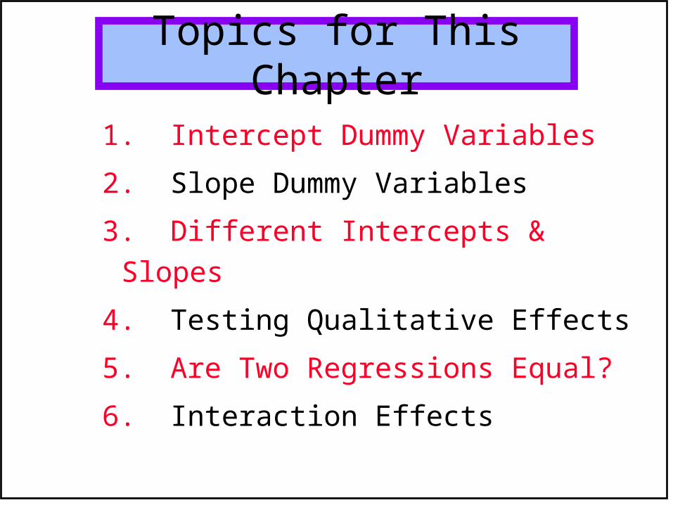
2Topics for This Chapter

1. Intercept Dummy Variables

2. Slope Dummy Variables

3. Different Intercepts & Slopes

4. Testing Qualitative Effects

5. Are Two Regressions Equal?

6. Interaction Effects

3Dummy variablesDummy variables, often called binary or

dichotomous variables, are explanatory variables that only take two values, usually 0 and 1.

These simple variables are a very powerful tool for capturing qualitative characteristics of individuals, such as gender, race, geographic region of residence.

In general, we use dummy variables to describe any event that has only two possible outcomes.

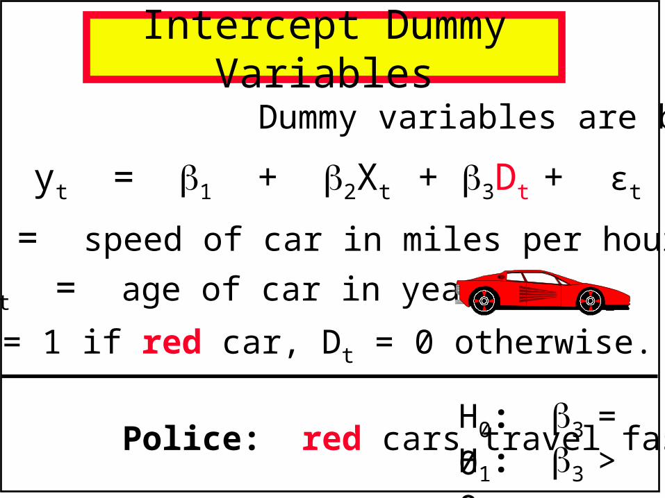
4Intercept Dummy Variables

Dummy variables are binary (0,1)

Dt = 1 if red car, Dt = 0 otherwise.

yt = 1 + 2Xt + 3Dt + εt

yt = speed of car in miles per hour

Xt = age of car in years

Police: red cars travel faster.H0: 3 = 0H1: 3 > 0

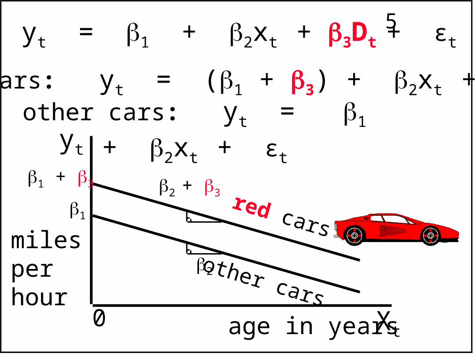
5yt = 1 + 2xt + 3Dt + εt

red cars: yt = (1 + 3) + 2xt + εt other cars: yt = 1 + 2xt + εt

yt

Xt

milesper hour

age in years0

1 + 3

1

2 + 3

2

red cars

other cars

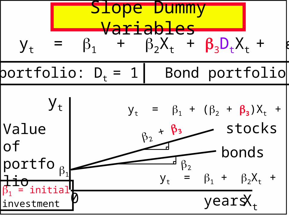
6Slope Dummy Variables

yt = 1 + 2Xt + 3DtXt + εt

yt = 1 + (2 + 3)Xt + εt

yt = 1 + 2Xt + εt

yt

Xt

Value ofportfolio

years0

2 + 3

12

stocks

bonds

Stock portfolio: Dt = 1 Bond portfolio: Dt = 0

1 = initial

investment

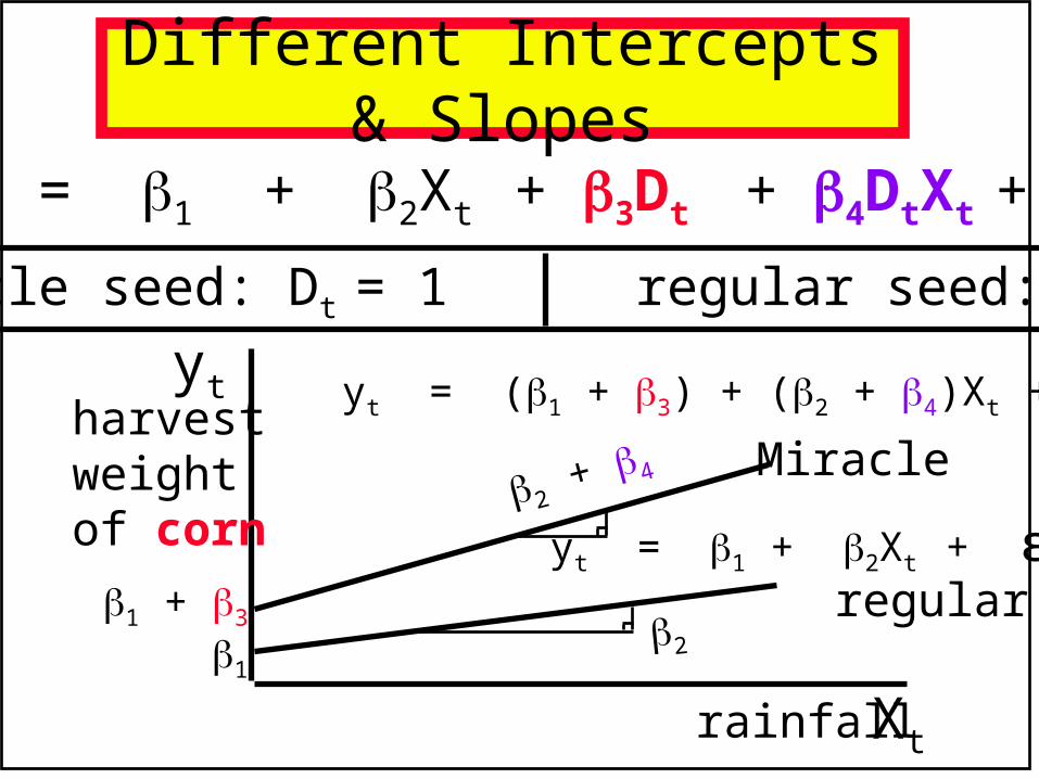
7Different Intercepts & Slopes

yt = 1 + 2Xt + 3Dt + 4DtXt + εt

yt = (1 + 3) + (2 + 4)Xt + εt

yt = 1 + 2Xt + εt

yt

Xt

harvestweightof corn

rainfall

2 + 4

12

Miracle

regular

Miracle seed: Dt = 1 regular seed: Dt = 0

1 + 3

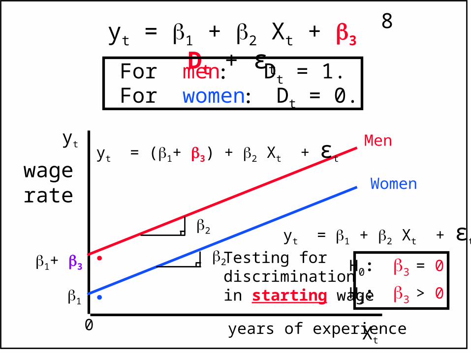
8yt = 1 + 2 Xt + 3 Dt + εt

21+ 3

2

1

yt

Xt

Men

Women

0

yt = 1 + 2 Xt + εt

For men Dt = 1. For women Dt = 0.

years of experience

yt = (1+ 3) + 2 Xt + εt

wagerate

H0: 3 = 0

H1: 3 > 0 .

. Testing fordiscriminationin starting wage

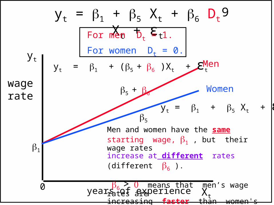
9yt = 1 + 5 Xt + 6 Dt Xt + εt

5

5 +6

1

yt

Xt

Men

Women

0

yt = 1 + (5 +6 )Xt + εt

yt = 1 + 5 Xt + εt

For men Dt = 1.

For women Dt = 0.

Men and women have the same starting wage, 1 , but their wage ratesincrease at different rates (different 6 ).

6 > means that men’s wage rates areincreasing faster than women's wage rates.

years of experience

wagerate

10

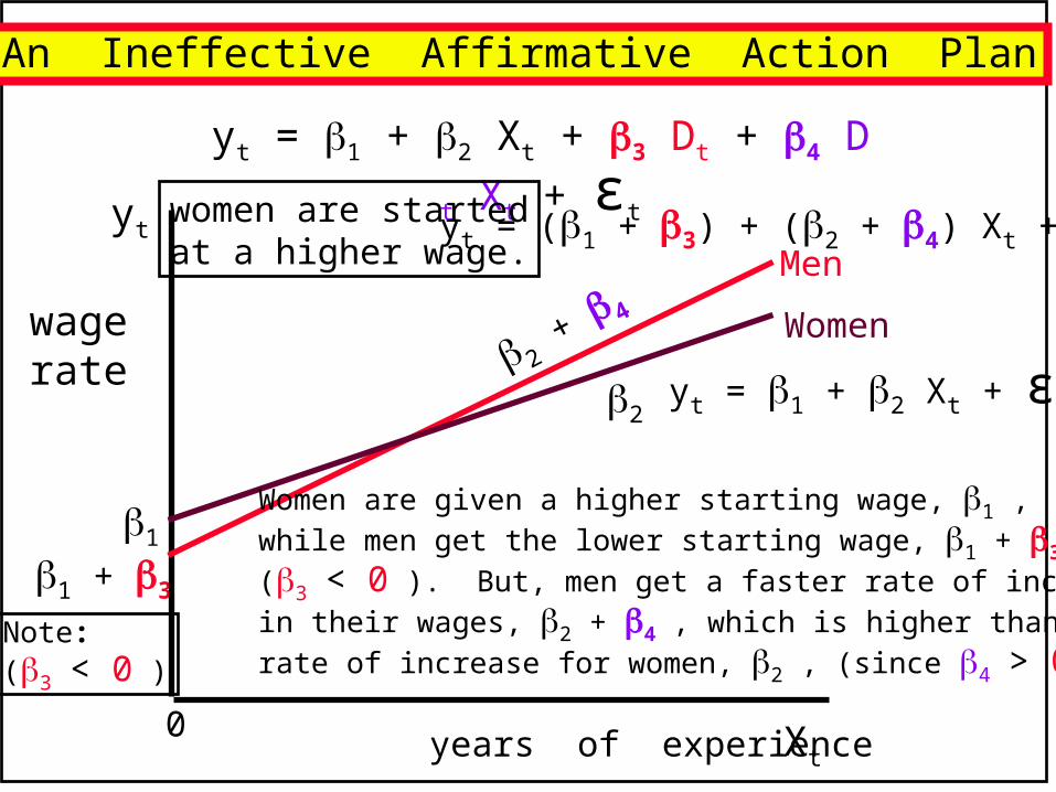
yt = 1 + 2 Xt + 3 Dt + 4 Dt Xt + εt

1 + 3

1

2

2 + 4

yt

Xt

Men

Women

0

yt = (1 + 3) + (2 + 4) Xt + εt

yt = 1 + 2 Xt + εt

Women are given a higher starting wage, 1 , while men get the lower starting wage, 1 + 3 ,(3 < 0 ). But, men get a faster rate of increasein their wages, 2 + 4 , which is higher than therate of increase for women, 2 , (since 4 > 0 ).

years of experience

An Ineffective Affirmative Action Plan

women are startedat a higher wage.

Note:(3 < 0 )

wagerate

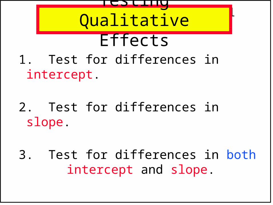
11Testing Qualitative Effects

1. Test for differences in intercept.

2. Test for differences in slope.

3. Test for differences in both intercept and slope.

12

H0: vs1:

H0: vs1:

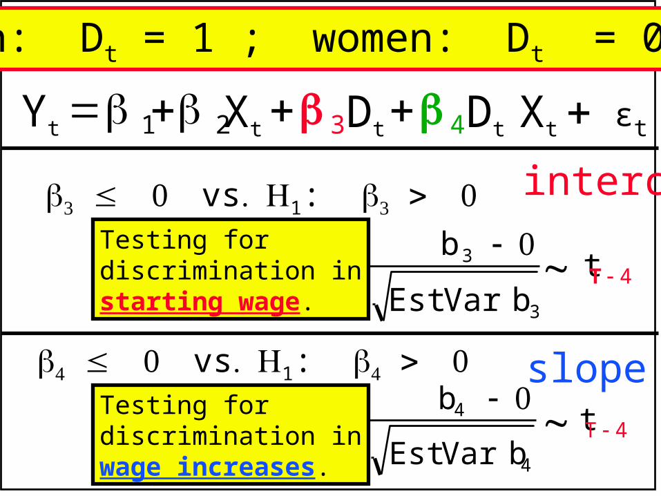
Yt 12Xt3Dt

4Dt Xt

b3

Est .Var b3tT 4

b4

Est .Var b4tT 4

men: Dt = 1 ; women: Dt = 0

Testing fordiscrimination instarting wage.

Testing fordiscrimination inwage increases.

intercept

slope

εt

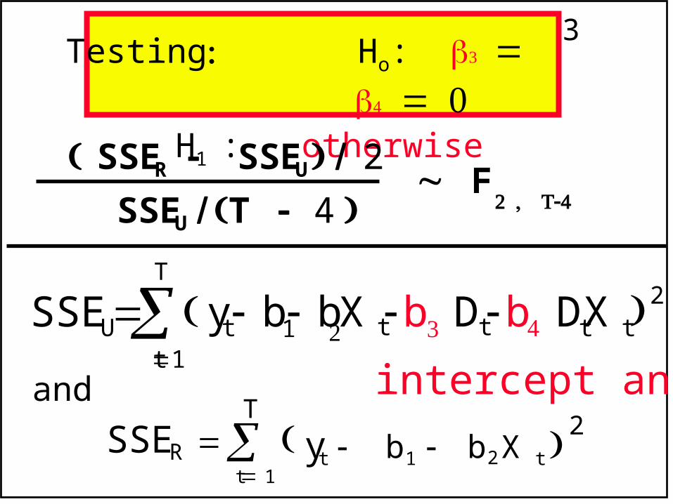
13Testing Ho:

H1 : otherwise

and

SSER yt b1 b2X t 2

t 1

T

SSEU yt b1 bX tb Dtb DtX t2

t1

T

SSER SSEU 2

SSEU T 4 F

intercept and slope

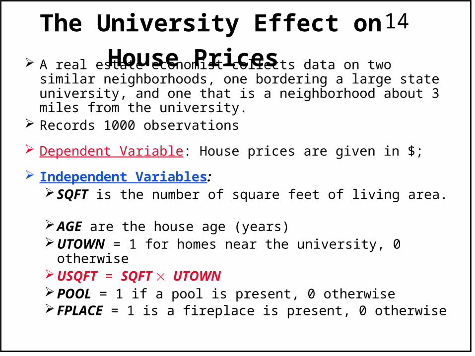
14 The University Effect on House Prices A real estate economist collects data on two similar

neighborhoods, one bordering a large state university, and one that is a neighborhood about 3 miles from the university.

Records 1000 observations

Dependent Variable: House prices are given in $;

Independent Variables:SQFT is the number of square feet of living area. AGE are the house age (years)UTOWN = 1 for homes near the university, 0 otherwiseUSQFT = SQFT UTOWNPOOL = 1 if a pool is present, 0 otherwiseFPLACE = 1 is a fireplace is present, 0 otherwise  

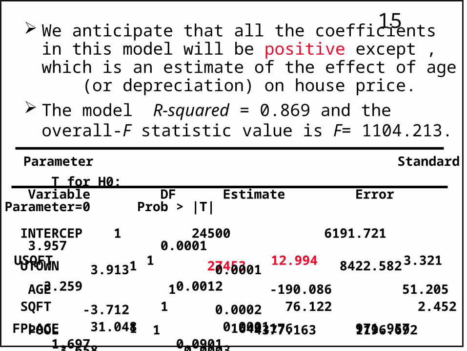
15 We anticipate that all the coefficients in this model will be positive except , which is an estimate of the effect of age (or depreciation) on house price.

The model R-squared = 0.869 and the overall-F statistic value is F= 1104.213.

 

Parameter Standard T for H0: Variable DF Estimate Error Parameter=0 Prob > |T|  INTERCEP 1 24500 6191.721 3.957 0.0001

UTOWN 1 27453 8422.582 3.259 0.0012

SQFT 1 76.122 2.452 31.048 0.0001

USQFT 1 12.994 3.321 3.913 0.0001

AGE 1 -190.086 51.205 -3.712 0.0002

POOL 1 4377.163 1196.692 3.658 0.0003

FPLACE 1 1649.176 971.957 1.697 0.0901

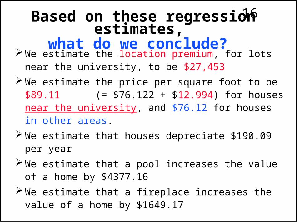
16Based on these regression estimates, what do we conclude?

We estimate the location premium, for lots near the university, to be $27,453

We estimate the price per square foot to be $89.11 (= $76.122 + $12.994) for houses near the university, and $76.12 for houses in other areas.

We estimate that houses depreciate $190.09 per year

We estimate that a pool increases the value of a home by $4377.16

We estimate that a fireplace increases the value of a home by $1649.17

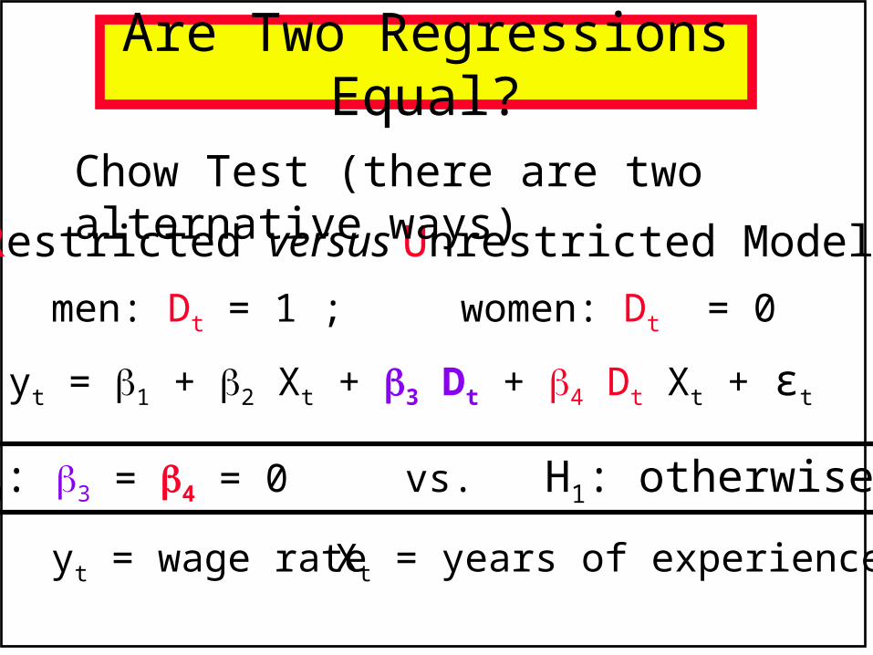
17Are Two Regressions Equal?

yt = 1 + 2 Xt + 3 Dt + 4 Dt Xt + εt

I. Restricted versus Unrestricted Models

men: Dt = 1 ; women: Dt = 0

H0: 3 = 4 = 0 vs. H1: otherwise

yt = wage rate Xt = years of experience

Chow Test (there are two alternative ways)

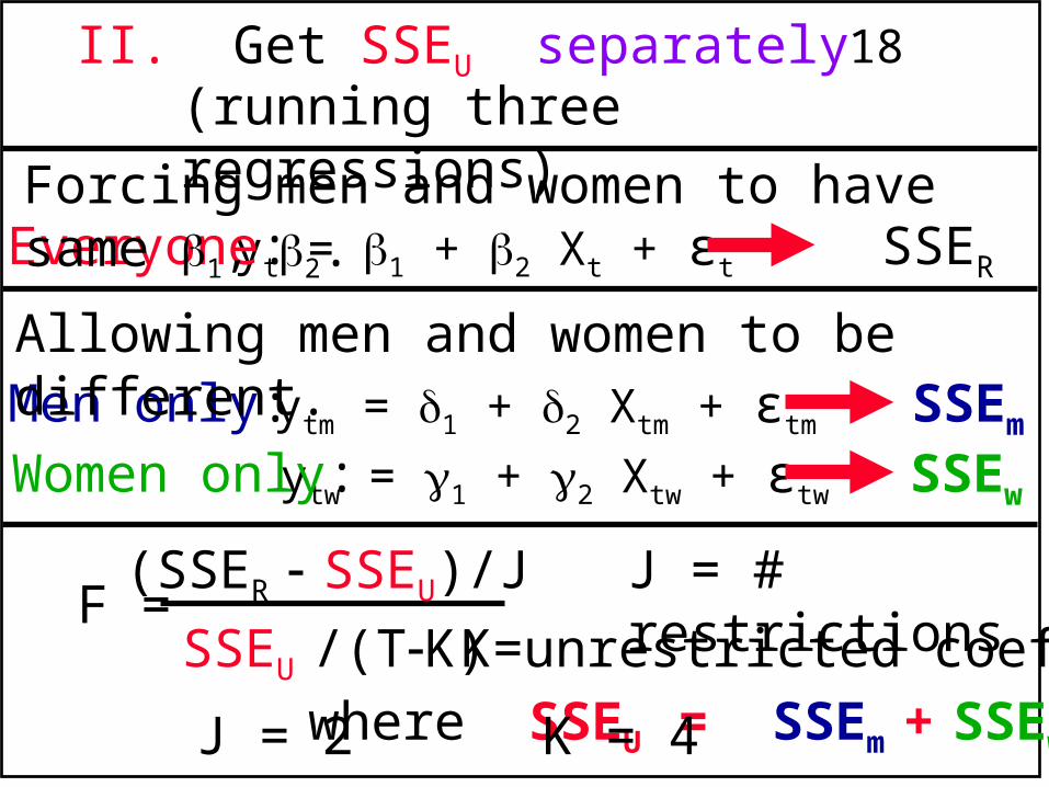
18

yt = 1 + 2 Xt + εt

II. Get SSEU separately

ytm = 1 + 2 Xtm + εtm

ytw = 1 + 2 Xtw + εtw

Everyone:

Men only:Women only:

SSER

Forcing men and women to have same 1, 2.

Allowing men and women to be different.SSEm

SSEw

where SSEU = SSEm + SSEw

F =(SSER SSEU)/J

SSEU /(TK)

J = # restrictions

K=unrestricted coefs.

(running three regressions)

J = 2 K = 4

19

Interaction Variables

1. Interaction Dummies

2. Polynomial Terms

(special case of continuous interaction)

3. Interaction Among Continuous Variables

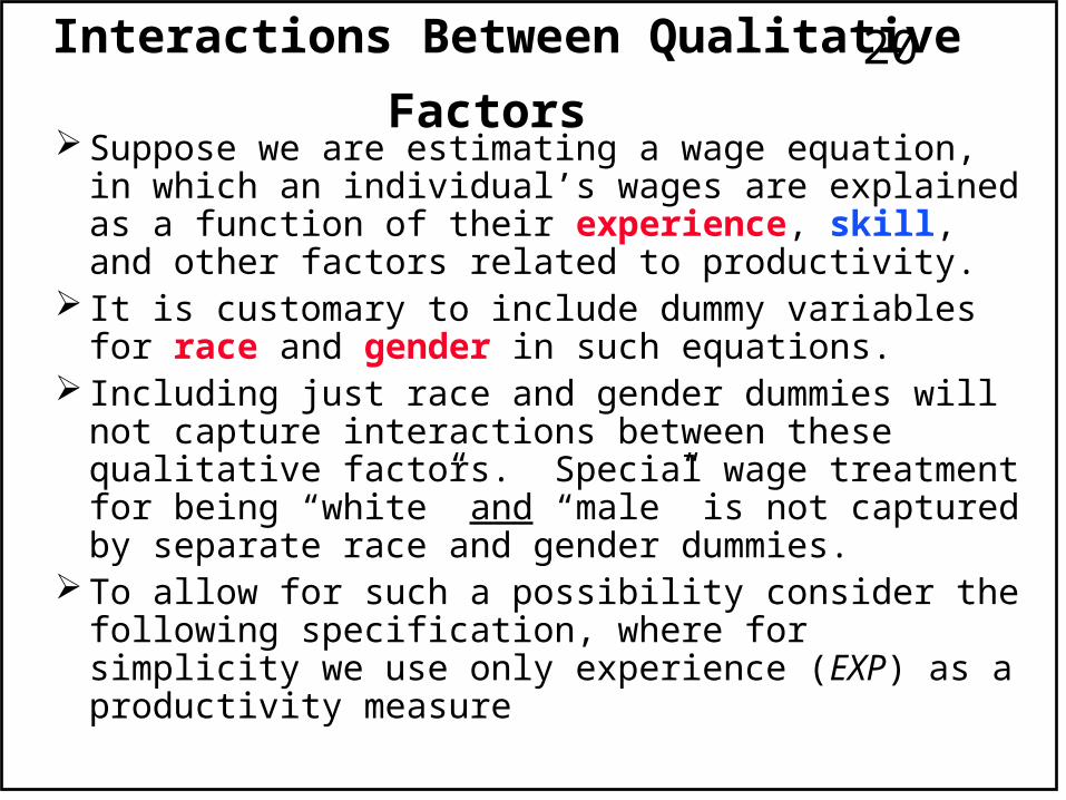
20Interactions Between Qualitative Factors Suppose we are estimating a wage equation, in which

an individual’s wages are explained as a function of their experience, skill, and other factors related to productivity.

It is customary to include dummy variables for race and gender in such equations.

Including just race and gender dummies will not capture interactions between these qualitative factors. Special wage treatment for being “white” and “male” is not captured by separate race and gender dummies.

To allow for such a possibility consider the following specification, where for simplicity we use only experience (EXP) as a productivity measure

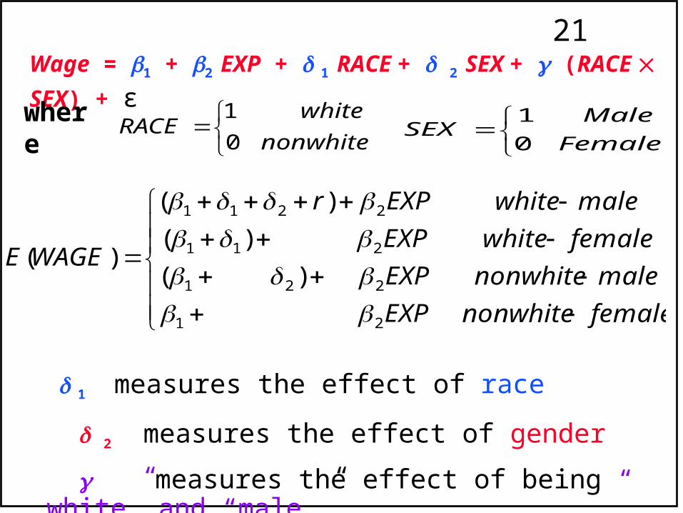
21Wage = 1 + 2 EXP + 1 RACE + 2 SEX + (RACE SEX) + ε

where

nonwhite

whiteRACE

0

1

Female

MaleSEX

0

1

femalenonwhite

malenonwhite

femalewhite

malewhite

EXP

EXP

EXP

EXPr

WAGEE

21

221

211

2211

)(

)(

)(

)(

1 measures the effect of race

2 measures the effect of gender

measures the effect of being “white” and “male.”

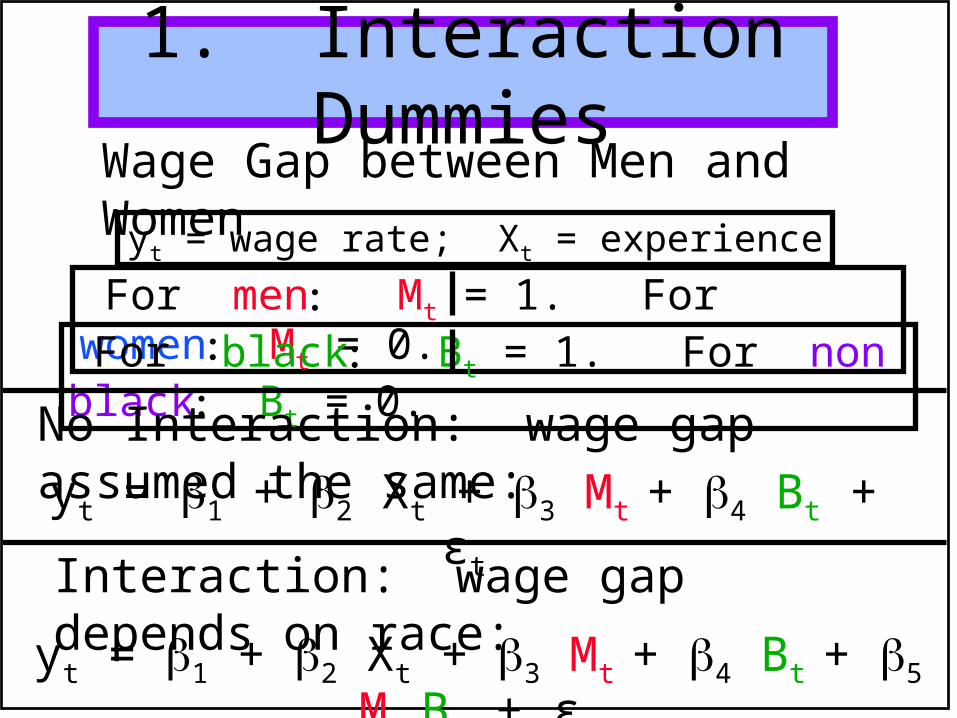
221. Interaction Dummies

yt = 1 + 2 Xt + 3 Mt + 4 Bt + εt

For men Mt = 1. For women Mt = 0. For black Bt = 1. For nonblack Bt = 0.

No Interaction: wage gap assumed the same:

yt = 1 + 2 Xt + 3 Mt + 4 Bt + 5 Mt Bt + εt

Interaction: wage gap depends on race:

Wage Gap between Men and Women

yt = wage rate; Xt = experience

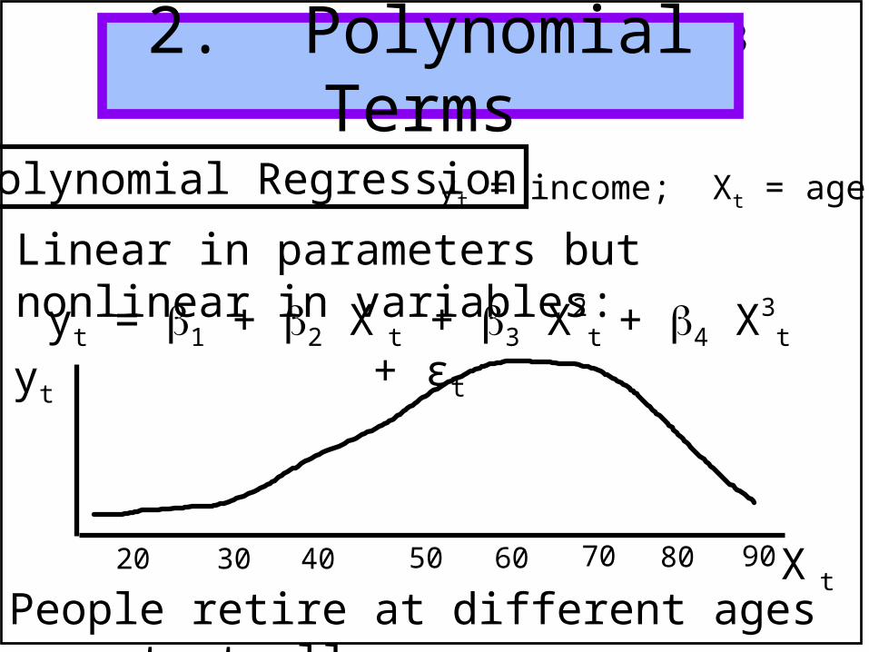
232. Polynomial Terms

yt = 1 + 2 X t + 3 X2

t + 4 X3

t + εt

Linear in parameters but nonlinear in variables:

yt = income; Xt = agePolynomial Regression

yt

X tPeople retire at different ages or not at all.

9020 30 40 50 60 8070

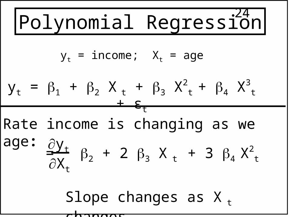
24

yt = 1 + 2 X t + 3 X2

t + 4 X3

t + εt

yt = income; Xt = age

Polynomial Regression

Rate income is changing as we age:yt

Xt

= 2 + 2 3 X t + 3 4 X

2t

Slope changes as X t changes.

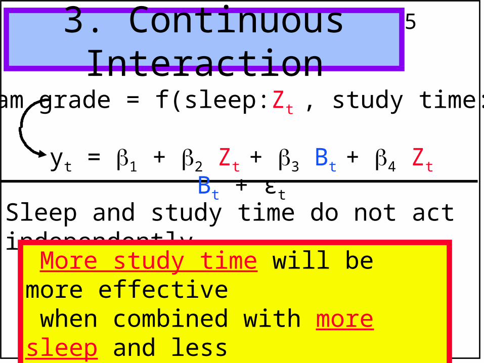
253. Continuous Interaction

yt = 1 + 2 Zt + 3 Bt + 4 Zt Bt + εt

Exam grade = f(sleep:Zt , study time:Bt)

Sleep and study time do not act independently.

More study time will be more effective when combined with more sleep and less effective when combined with less sleep.

26

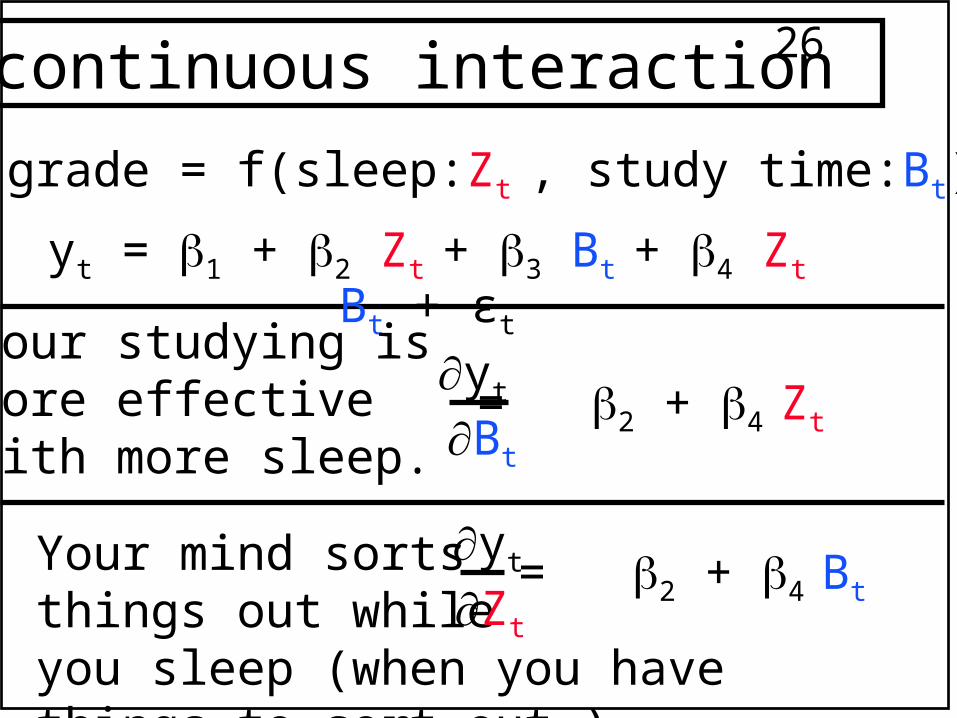
Your mind sortsthings out whileyou sleep (when you have things to sort out.)

yt = 1 + 2 Zt + 3 Bt + 4 Zt Bt + εt

Exam grade = f(sleep:Zt , study time:Bt)

yt

Bt

= 2 + 4 Zt

Your studying is more effectivewith more sleep.

yt

Zt

= 2 + 4 Bt

continuous interaction

27

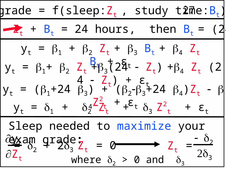
yt = 1 + 2 Zt + 3 Bt + 4 Zt Bt + εt

Exam grade = f(sleep:Zt , study time:Bt)

If Zt + Bt = 24 hours, then Bt = (24 Zt)

yt = 1+ 2 Zt +3(24 Zt) +4 Zt (24 Zt) + εt

yt = (1+24 3) + (23+24 4)Zt 4Z2

t + εt

yt = 1 + 2 Zt + 3 Z2

t + εt

Sleep needed to maximize your exam grade:yt

Zt

= 2 + 23 Zt = 0where 2 > 0 and 3 < 0

2

3

Zt =

28Qualitative Variables with Several Categories

Many qualitative factors have more than two categories.

Examples are region of the country (North, South, East, West) and level of educational attainment (less than high school, high school, college, postgraduate).

For each category we create a separate binary dummy variable.

To illustrate, let us again use a wage equation as an example, and focus only on experience and level of educational attainment (as a proxy for skill) as explanatory variables.

29

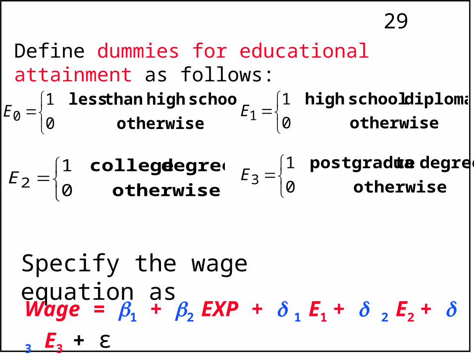
Define dummies for educational attainment as follows:

otherwise

diploma school high

0

11E

otherwise

school high than less

0

10E

otherwise

degree college

0

12E

otherwise

degree tepostgradua

0

13E

Specify the wage equation as

Wage = 1 + 2 EXP + 1 E1 + 2 E2 + 3 E3 + ε

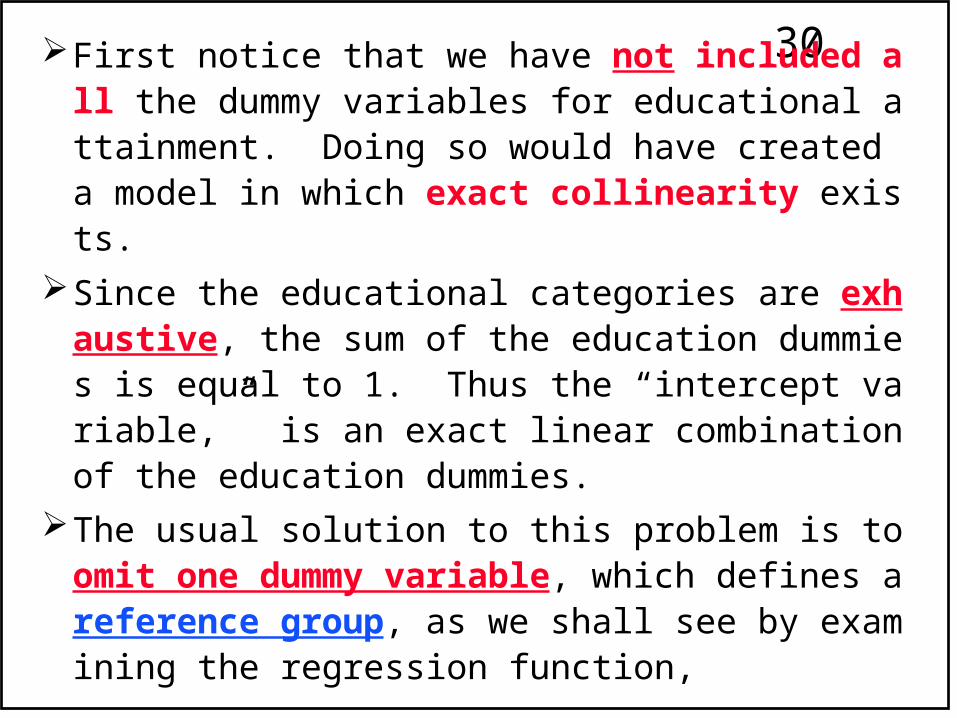
30First notice that we have not included all the dummy variables for educational attainment. Doing so would have created a model in which exact collinearity exists.

Since the educational categories are exhaustive, the sum of the education dummies is equal to 1. Thus the “intercept variable,” is an exact linear combination of the education dummies.

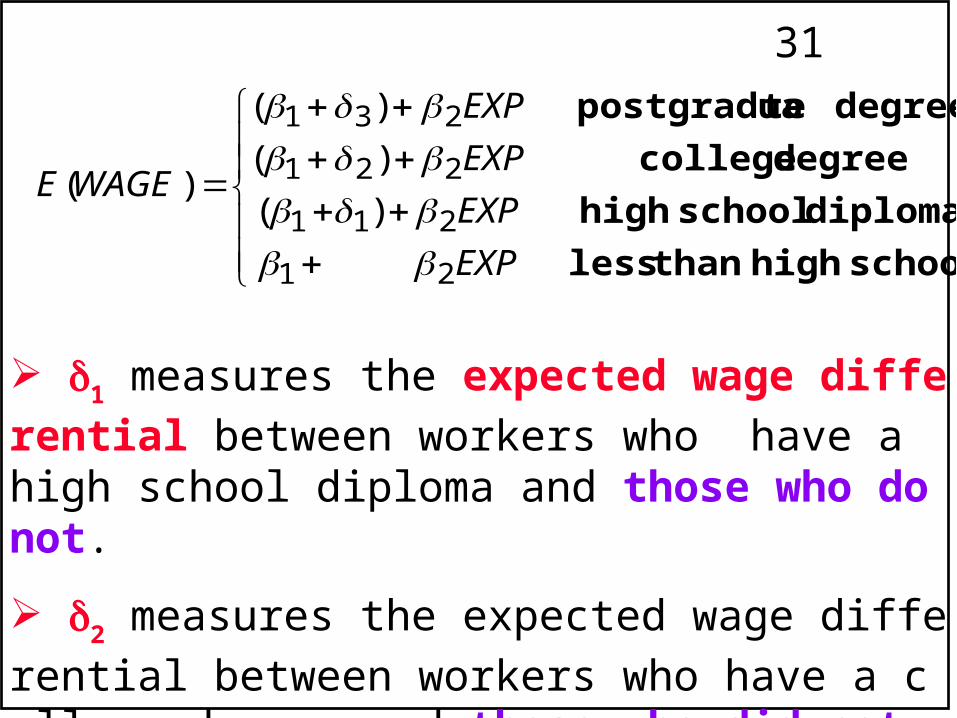
The usual solution to this problem is to omit one dummy variable, which defines a reference group, as we shall see by examining the regression function,

31

school high than less

diploma school high

degree college

degree tepostgradua

EXP

EXP

EXP

EXP

WAGEE

21

211

221

231

)(

)(

)(

)(

1 measures the expected wage differential betwee

n workers who have a high school diploma and those who do not.

2 measures the expected wage differential between

workers who have a college degree and those who did not graduate from high school, and so on.

32 The omitted dummy variable, E0, identifies those who

did not graduate from high school. The coefficients of the dummy variables represent expected wage differentials relative to this group.

The intercept parameter 1 represents the base wage for a worker with no experience and no high school diploma.

Mathematically it does NOT matter which dummy variable is omitted, although the choice of E0 is convenient in the example above.

If we are estimating an equation using geographic dummy variables, N, S, E and W, identifying regions of the country, the choice of which dummy variable to omit is arbitrary.