1

Dynamic Scene Deblurring usinga Locally Adaptive Linear Blur Model

Tae Hyun Kim, Seungjun Nah, and Kyoung Mu Lee

Abstract—State-of-the-art video deblurring methods cannot handle blurry videos recorded in dynamic scenes, since they are builtunder a strong assumption that the captured scenes are static. Contrary to the existing methods, we propose a video deblurringalgorithm that can deal with general blurs inherent in dynamic scenes. To handle general and locally varying blurs caused by varioussources, such as moving objects, camera shake, depth variation, and defocus, we estimate pixel-wise non-uniform blur kernels. Weinfer bidirectional optical flows to handle motion blurs, and also estimate Gaussian blur maps to remove optical blur from defocus in ournew blur model. Therefore, we propose a single energy model that jointly estimates optical flows, defocus blur maps and latent frames.We also provide a framework and efficient solvers to minimize the proposed energy model. By optimizing the energy model, weachieve significant improvements in removing general blurs, estimating optical flows, and extending depth-of-field in blurry frames.Moreover, in this work, to evaluate the performance of non-uniform deblurring methods objectively, we have constructed a new realisticdataset with ground truths. In addition, extensive experimental on publicly available challenging video data demonstrate that theproposed method produces qualitatively superior performance than the state-of-the-art methods which often fail in either deblurring oroptical flow estimation.

Index Terms—video deblurring, non-uniform blur, motion blur, defocus blur, optical flow

F

1 INTRODUCTION

M OTION blurs are the most common artifacts in videosrecorded from hand-held cameras. In low-light conditions,

these blurs are caused by camera shake and object motions duringexposure time. In addition, fast moving objects in the scene causeblurring artifacts in a video even when the light conditions areacceptable. For decades, this problem has motivated considerableworks on deblurring and different approaches have been soughtdepending on whether the captured scenes are static or dynamic.

Early works on a single image deblurring problem are basedon assumptions that the captured scene is static and has constantdepth [1], [2], [3], [4], [5], [6] and they estimated uniform ornon-uniform blur kernel by camera shake. These approaches werenaturally extended to video deblurring methods. Cai et al. [7]proposed a deconvolution method with multiple frames usingsparsity of both blur kernels and clear images to reduce errorsfrom inaccurate registration and render high-quality latent image.However, this approach removes only uniform blur caused bytwo-dimensional translational camera motion, and the proposedapproach cannot handle non-uniform blur from rotational cameramotion around z-axis, which is the main cause of motion blurs [6].To solve this problem, Li et al. [8] adopted a method parameter-izing spatially varying motions with 3x3 homographies based onthe previous work of Tai et al. [9], and could handle non-uniformblurs by rotational camera shake. In the work of Cho et al. [10],camera motion in three-dimensional space was estimated withoutany assistance of specialized hardware, and spatially varying blurscaused by projective camera motion were obtained. Moreover, inthe works of Paramanand et al. [11] and Lee and Lee [12], spatially

• The authors are with the Department of Electrical Engineering and Com-puter Science, Automation and Systems Research Institute, Seoul NationalUniversity, 1 Ganak-ro, Gwanak-gu, Seoul 151-744, South Korea (E-mail:lliger9@snu.ac.kr, seungjun.nah@gmail.com, kyoungmu@snu.ac.kr).

varying blurs by depth variation in a static scene were estimatedand removed.

However, these previous methods, which assume static scene,suffer from spatially varying blurs from not only camera shakebut also moving objects in a dynamic scene. Because it is difficultto parameterize the pixel-wise varying blur kernel in the dynamicscene with simple homography, kernel estimation becomes morechallenging task. Therefore, several researchers have studied onremoving blurs in dynamic scenes, which are grouped into two ap-proaches: segmentation-based deblurring approach, and exemplar-based deblurring approach.

Segmentation-based approaches usually estimate multiple mo-tions, kernels, and associated segments. In the work of Choet al. [13], a method that segments homogeneous motions andestimates segment-wise different 1D Gaussian blur kernels, wasproposed. However, it cannot handle complex motions by rota-tional camera shakes due to the limitation of Gaussian kernels.In the work of Bar et al. [14], a layered model was proposedthat segments images into foreground and background layers, andestimates a linear blur kernel within the foreground layer. By usingthe layered model, explicit occlusion handling is possible, butthe kernel is restricted to linear. To overcome these limitations,Wulff and Black [15] improved the previous layered model ofBar et al. by estimating the different motions of both foregroundand background layers. However, these motions are restricted toaffine models and it is difficult to extend to multi-layered scenesbecause such task requires depth ordering of the layers. To sumup, segmentation-based deblurring approaches have the advantageof removing blurs caused by moving objects in dynamic scenes.However, segmentation itself is very difficult problem and remainsstill an challenging issue as reported in [16]. Moreover, they fail tosegment complex motions like motions of people, because simpleparametric motion models used in [14], [15] cannot fit the complexmotions accurately.

arX

iv:1

603.

0426

5v1

[cs

.CV

] 1

4 M

ar 2

016

2

(a) (b) (c)

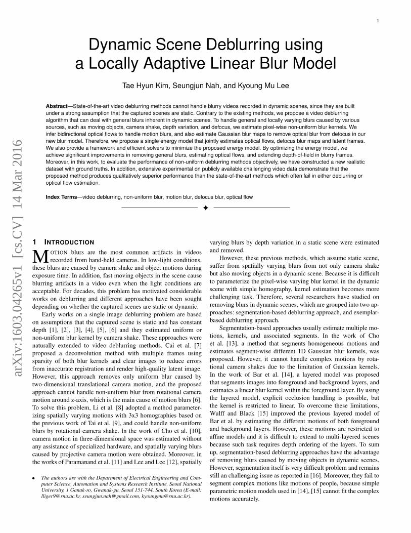
Fig. 1: (a) A Blurry frame in a dynamic scene. (b) Our deblurring result. (c) Our color coded optical flow estimation result.

Exemplar-based approaches were proposed in the works ofMatsushita et al. [17] and Cho et al. [18]. These methods usuallydo not rely on accurate segmentation and deconvolution. Instead,the latent frames are rendered by interpolating lucky sharp framesthat frequently exist in videos, thus avoiding severe ringing arti-facts. However, the work of Matsushita et al. [17] cannot removeblurs caused by moving objects. In addition the work of Choet al. [18] allows only slow-moving objects in dynamic scenesbecause it searches sharp patches corresponding to blurry patchafter registration with homography. Therefore, it cannot handlefast moving objects which have distinct motions from those ofbackgrounds. Moreover, since it does not use deconvolution withspatial priors but simple interpolation, it degrades mid-frequencytextures such as grasses and trees, and renders smooth results.

On the other hand, defocus from limited depth-of-field (DOF)of conventional digital cameras also results in blurry effects invideos. Although shallow DOF is often used to render aestheticimages and highlight the focused objects, frequent misfocus ofmoving objects in video yields image degradation when themotion is large and fast. Moreover, depth variation in the scenegenerates spatially varying defocus blurs, making the estimation ofdefocus blur map is also a difficult problem. Thus many researcheshave studied to estimate defocus blur kernel. Most of them haveapproximated the kernel as simple Gaussian or disc model, makingthe kernel estimation problem becomes a parameter (e.g. standarddeviation of Gaussian blur, disc radius) estimation problem [19],[20], [21], [22].

To magnify focus differences, Bae and Durand [19] estimateddefocus blur map at the edges first, and then propagated theresults to other regions. However, the estimated blur map isinaccurate where the blurs are strong, since it is image-basedapproach and depends on the detected edges that can be localized.Similarly, Zhuo and Sim [22] propagated the amount of blurat the edges to elsewhere, that obtained by measuring the ratiobetween the gradients of the defocused input and re-blurred inputwith a Gaussian kernel. To reduce reliance on strong edges inthe defocused image, Zhu et al. [21] utilized statistics of blurspectrum within the defocused image, since statistical modelscould be applicable where there are no strong edges. Specifically,local image statistics is used to measure the probability of defocusscale and determine the locally varying scale of defocus blur ina single image. However, local image statistics-based methods donot work when there are motion blurs as well as defocus blurs

within a single image; Motion blurs change local statistics andyield much complex blurs combined with defocus blurs.

In the recent work of Kim and Lee [23], a new and generalizedvideo deblurring (GVD) method that estimates latent frameswithout using global motion parametrization and segmentationwas proposed to remove motion blurs in dynamic scenes. In GVD,bidirectional optical flows are estimated and used to infer pixel-wise varying kernels. Therefore, the proposed method naturallyhandle coexisting blurs by camera shake, and moving objects withcomplex motions. Because estimating flow fields and restoringsharp frames are a joint problem, both variables are simultaneouslyestimated in GVD. To do so, a new single energy model to solvethe joint problem was proposed and efficient solvers to optimizethe model is provided.

However, since GVD method is based on piece-wise linearkernel approximation, it cannot handle non-linear blurs combinedwith motion and defocus blurs which are common in videos cap-tured from hand-held cameras. Therefore, in this work, we proposean extended and more generalized method of GVD that can handlenot only motion blur but also defocus blur which further improvesthe deblurring quality significantly. Under an assumption that, thecomplex non-linear blur kernel can be decomposed into motionand defocus blur kernels, we estimate bidirectional optical flowsto approximate motion blur kernel, scales of Gaussian blurs toapproximate defocus blur kernel, and the latent frames jointly. Theresult of our system is shown in Fig.1, in which the motion blurs ofdifferently moving people and Gaussian blurs in the backgroundare successfully removed and accurate optical flows are jointlyestimated.

Finally, we provide a new realistic blur dataset with groundtruth sharp frames captured by a high-speed camera to overcomethe lack of realistic ground truth dataset in this field. Thoughthere have been some evaluation datasets for deblurring problem,they are not appropriate to carry out meaningful evaluation for thedeblurring of spatially varying blurs. First, synthetically generateduniform blur kernels and blurry images from sharp images wereprovided in the work of Levin et al. [24]. Next, 6D camera motionin 3D space was recorded with a hardware-assisted camera torepresent blur from camera shake during exposure time in thework of Kohler et al. [25]. Moreover, there have been some recentapproaches to generate synthetic dataset for the sake of machinelearning algorithms. To benefit from large training data, lots ofblur kernels and blurry images were synthetically generated. In the

KIM et al.: DYNAMIC SCENE DEBLURRING USING A LOCALLY ADAPTIVE LINEAR BLUR MODEL 3

(a) (b) (c)

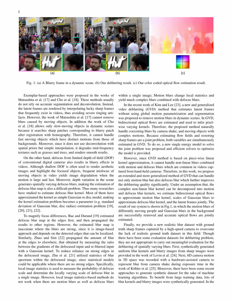
Fig. 2: (a) Blurry frame from a dynamic scene. (b) Deblurring result by Cho et al. [18]. (c) Our result.

work of Xu et al. [26], more than 2500 blurry images are generatedusing decomposable symmetric kernels. Schuler et al. [27] sam-pled naturally looking blur kernels with Gaussian Process, and Sunet al. [28] used a set of linear kernels to synthesize blurry images.However, these datasets are generated under an assumption thatthe scene is static and cannot synthesize infinitely many blurs inreal world. Real blurs in dynamic scenes are complex and spatiallyvarying, so synthesizing realistic dataset is a difficult problem. Tosolve this problem, we construct a new blur dataset that providespairs of realistically blurred videos and sharp videos with the useof a high-speed camera.

Using the proposed dataset and real challenging videos asshown in Fig.2, we demonstrate the significant improvementsof the proposed deblurring method in both quantitatively andqualitatively. Moreover, we show empirically that more accurateoptical flows are estimated by our method compared with the state-of-the-art optical flow method that can handle blurry images.

2 MORE GENERALIZED VIDEO DEBLURRING

Most conventional video deblurring methods suffer from the coex-istence of various motion blurs from dynamic scenes because themotions cannot be fully parameterized using global or segment-wise blur models. To make things worse, frequent misfocus ofmoving objects in dynamic scenes yields more complex non-linearblurs combined with motion blurs.

To handle these joint motion and defocus blurs, we propose anew blur model that estimates locally (pixel-wise) different blurkernels rather than global or segment-wise kernel estimation. Asblind deblurring problem is highly ill-posed, we propose a singleenergy model consists of not only data and spatial regularizationterms but also a temporal term. The model is expressed as follows:

E = Edata + Etemporal + Espatial, (1)

and the detailed models of each term in (1) are given in thefollowing sections.

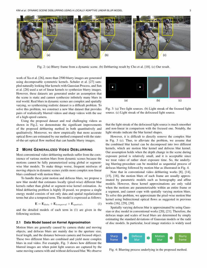
2.1 Data Model based on Kernel ApproximationMotion blurs are generally caused by camera shake and movingobjects, and defocus blurs are mainly due to the aperture size,focal length, and the distance between camera and focused object.These two different blurs are combined and yield more complexblurs in real video. For example, Fig. 3 shows how different theblurred images are when point light sources are captured by thesame moving camera with and without defocused blur. We observe

(a) (b) (c)

Fig. 3: (a) Two light sources. (b) Light streak of the focused lightsource. (c) Light streak of the defocused light source.

that the light streak of the defocused light source is much smootherand non-linear in comparison with the focused one. Notably, thelight streaks indicate the blur kernel shapes.

However, it is difficult to directly remove the complex blurin Fig. 3 (c). Thus, to alleviate the problem, we assume thatthe combined blur kernel can be decomposed into two differentkernels, which are motion blur kernel and defocus blur kernel.Our assumption holds when the depth change in the scene duringexposure period is relatively small, and it is acceptable sincewe treat video of rather short exposure time. So, the underly-ing blurring-procedure can be modeled as sequential process ofdefocus blurring followed by motion blur as illustrated in Fig. 4.

Note that in conventional video deblurring works [8], [14],[15], [18], the motion blurs of each frame are usually approx-imated by parametric models such as homography and affinemodels. However, these kernel approximations are only validwhen the motions are parameterizable within an entire frame ora segment, and cannot cope with spatially varying motion blurs.To solve this problem, we approximate the pixel-wise motion blurkernel using bidirectional optical flows as suggested in previousworks [16], [29], [30].

Spatially varying defocus blur is approximated by using Gaus-sian or disc model in conventional works [20], [21]. Therefore, thedefocus maps and scales of local blurs are determined by simplyestimating the standard deviations of Gaussian models or the radiiof disc models. In particular, local image statistics is widely used

Sharp frame

Defocus blur

Motion blur

Blurry frame

Fig. 4: Blurring process underlying in the proposed method.

4

-30

-25

-20

-15

-10

-5

0

1 2 3 4 5 6 7 8 9 10

Log

likel

iho

od

Scales of defocus blur

Defocus blur only

Defocus + Motion Blur

(a) (b) (c)

(d)

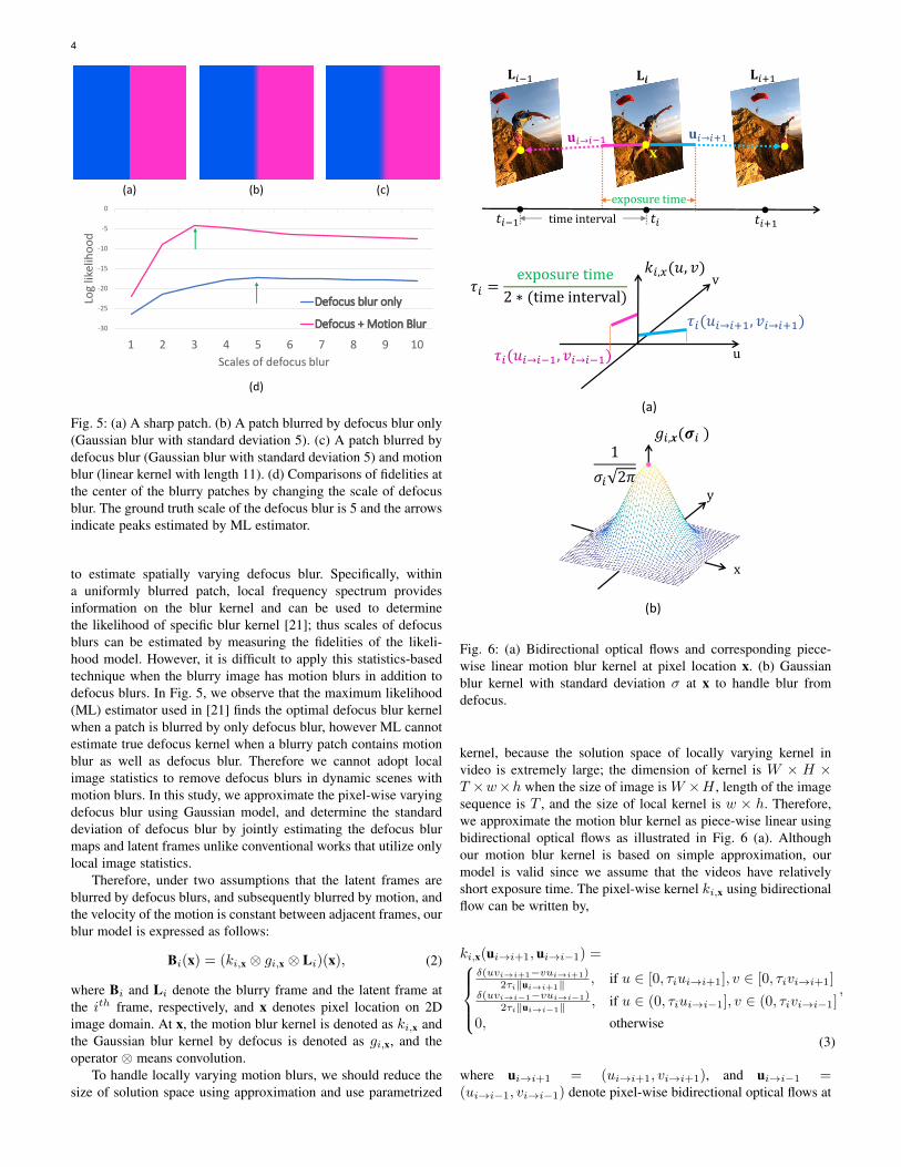
Fig. 5: (a) A sharp patch. (b) A patch blurred by defocus blur only(Gaussian blur with standard deviation 5). (c) A patch blurred bydefocus blur (Gaussian blur with standard deviation 5) and motionblur (linear kernel with length 11). (d) Comparisons of fidelities atthe center of the blurry patches by changing the scale of defocusblur. The ground truth scale of the defocus blur is 5 and the arrowsindicate peaks estimated by ML estimator.

to estimate spatially varying defocus blur. Specifically, withina uniformly blurred patch, local frequency spectrum providesinformation on the blur kernel and can be used to determinethe likelihood of specific blur kernel [21]; thus scales of defocusblurs can be estimated by measuring the fidelities of the likeli-hood model. However, it is difficult to apply this statistics-basedtechnique when the blurry image has motion blurs in addition todefocus blurs. In Fig. 5, we observe that the maximum likelihood(ML) estimator used in [21] finds the optimal defocus blur kernelwhen a patch is blurred by only defocus blur, however ML cannotestimate true defocus kernel when a blurry patch contains motionblur as well as defocus blur. Therefore we cannot adopt localimage statistics to remove defocus blurs in dynamic scenes withmotion blurs. In this study, we approximate the pixel-wise varyingdefocus blur using Gaussian model, and determine the standarddeviation of defocus blur by jointly estimating the defocus blurmaps and latent frames unlike conventional works that utilize onlylocal image statistics.

Therefore, under two assumptions that the latent frames areblurred by defocus blurs, and subsequently blurred by motion, andthe velocity of the motion is constant between adjacent frames, ourblur model is expressed as follows:

Bi(x) = (ki,x ⊗ gi,x ⊗ Li)(x), (2)

where Bi and Li denote the blurry frame and the latent frame atthe ith frame, respectively, and x denotes pixel location on 2Dimage domain. At x, the motion blur kernel is denoted as ki,x andthe Gaussian blur kernel by defocus is denoted as gi,x, and theoperator ⊗ means convolution.

To handle locally varying motion blurs, we should reduce thesize of solution space using approximation and use parametrized

𝐋𝑖−1 𝐋𝒊 𝐋𝑖+1

𝐮𝑖→𝑖+1

𝜏𝑖 =exposure time

2 ∗ (time interval)

𝐱

u

𝑘𝑖,𝑥(𝑢, 𝑣)v

𝜏𝑖(𝑢𝑖→𝑖+1, 𝑣𝑖→𝑖+1)

𝜏𝑖(𝑢𝑖→𝑖−1, 𝑣𝑖→𝑖−1)

𝑡𝑖−1 𝑡𝑖 𝑡𝑖+1time interval

exposure time

(a)

(b)

𝑔𝑖,𝒙(𝝈𝑖 )

x

y

1

𝜎𝑖 2𝜋

Fig. 6: (a) Bidirectional optical flows and corresponding piece-wise linear motion blur kernel at pixel location x. (b) Gaussianblur kernel with standard deviation σ at x to handle blur fromdefocus.

kernel, because the solution space of locally varying kernel invideo is extremely large; the dimension of kernel is W × H ×T ×w×h when the size of image is W ×H , length of the imagesequence is T , and the size of local kernel is w × h. Therefore,we approximate the motion blur kernel as piece-wise linear usingbidirectional optical flows as illustrated in Fig. 6 (a). Althoughour motion blur kernel is based on simple approximation, ourmodel is valid since we assume that the videos have relativelyshort exposure time. The pixel-wise kernel ki,x using bidirectionalflow can be written by,

ki,x(ui→i+1, ui→i−1) =δ(uvi→i+1−vui→i+1)

2τi‖ui→i+1‖ , if u ∈ [0, τiui→i+1], v ∈ [0, τivi→i+1]δ(uvi→i−1−vui→i−1)

2τi‖ui→i−1‖ , if u ∈ (0, τiui→i−1], v ∈ (0, τivi→i−1]

0, otherwise

,

(3)

where ui→i+1 = (ui→i+1, vi→i+1), and ui→i−1 =(ui→i−1, vi→i−1) denote pixel-wise bidirectional optical flows at

KIM et al.: DYNAMIC SCENE DEBLURRING USING A LOCALLY ADAPTIVE LINEAR BLUR MODEL 5

(c)

(a)

(b)

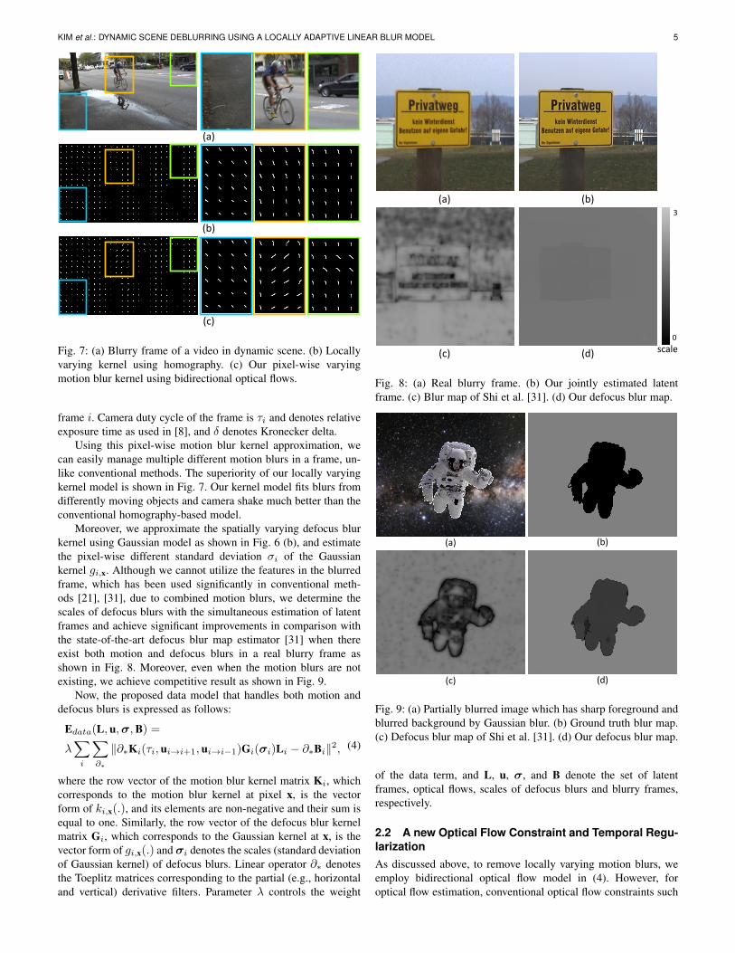
Fig. 7: (a) Blurry frame of a video in dynamic scene. (b) Locallyvarying kernel using homography. (c) Our pixel-wise varyingmotion blur kernel using bidirectional optical flows.

frame i. Camera duty cycle of the frame is τi and denotes relativeexposure time as used in [8], and δ denotes Kronecker delta.

Using this pixel-wise motion blur kernel approximation, wecan easily manage multiple different motion blurs in a frame, un-like conventional methods. The superiority of our locally varyingkernel model is shown in Fig. 7. Our kernel model fits blurs fromdifferently moving objects and camera shake much better than theconventional homography-based model.

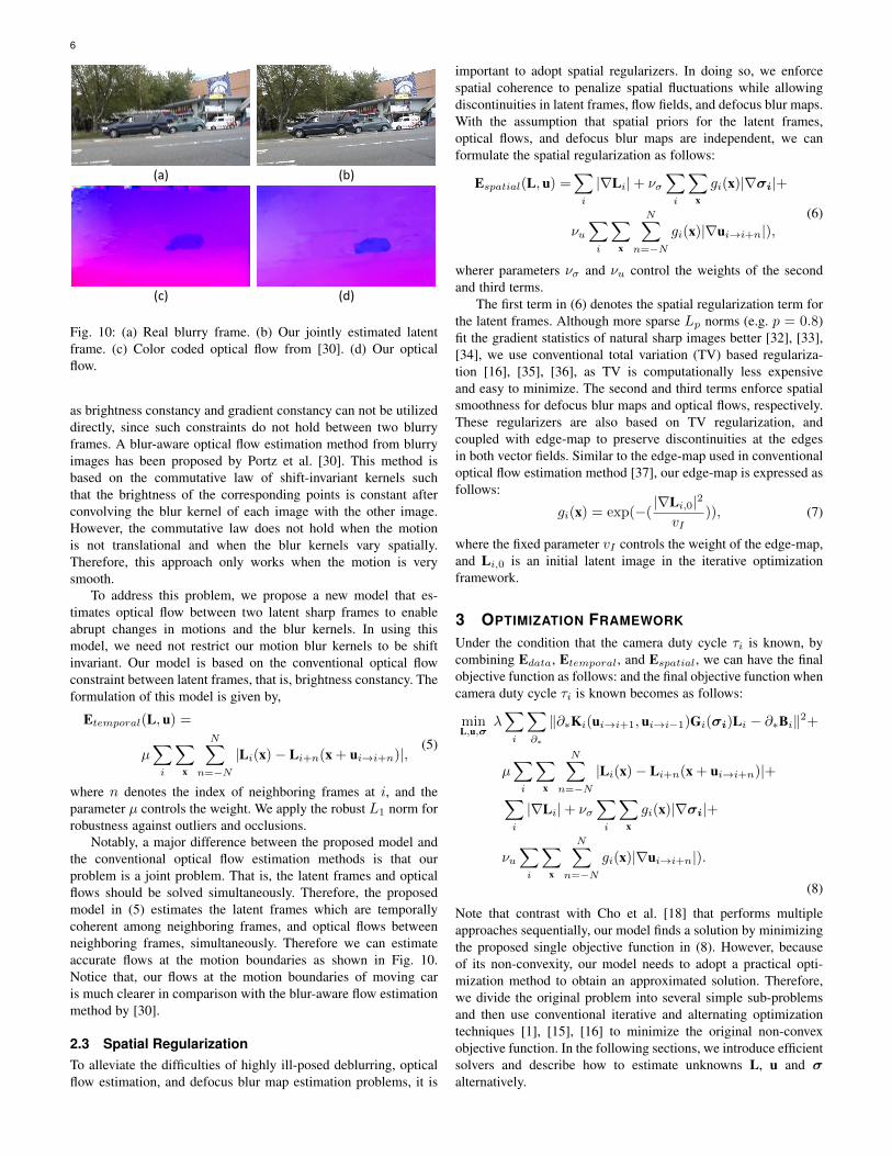
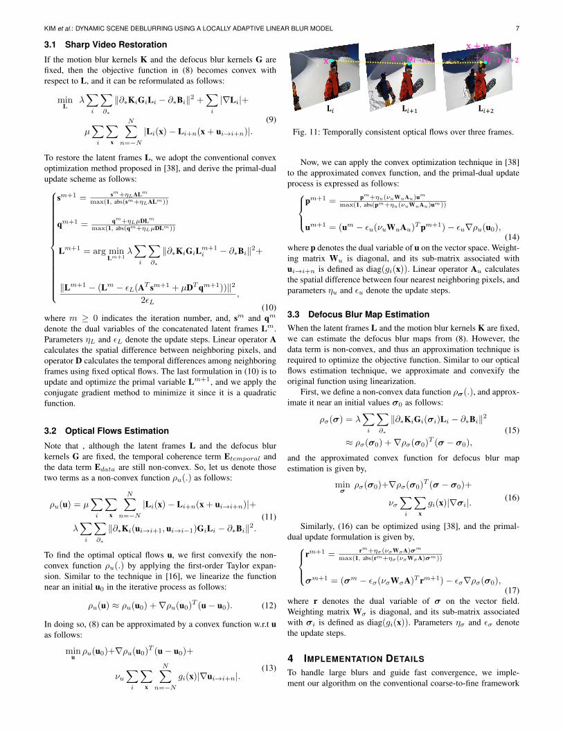
Moreover, we approximate the spatially varying defocus blurkernel using Gaussian model as shown in Fig. 6 (b), and estimatethe pixel-wise different standard deviation σi of the Gaussiankernel gi,x. Although we cannot utilize the features in the blurredframe, which has been used significantly in conventional meth-ods [21], [31], due to combined motion blurs, we determine thescales of defocus blurs with the simultaneous estimation of latentframes and achieve significant improvements in comparison withthe state-of-the-art defocus blur map estimator [31] when thereexist both motion and defocus blurs in a real blurry frame asshown in Fig. 8. Moreover, even when the motion blurs are notexisting, we achieve competitive result as shown in Fig. 9.

Now, the proposed data model that handles both motion anddefocus blurs is expressed as follows:

Edata(L, u,σ,B) =

λ∑i

∑∂∗

‖∂∗Ki(τi, ui→i+1, ui→i−1)Gi(σi)Li − ∂∗Bi‖2, (4)

where the row vector of the motion blur kernel matrix Ki, whichcorresponds to the motion blur kernel at pixel x, is the vectorform of ki,x(.), and its elements are non-negative and their sum isequal to one. Similarly, the row vector of the defocus blur kernelmatrix Gi, which corresponds to the Gaussian kernel at x, is thevector form of gi,x(.) and σi denotes the scales (standard deviationof Gaussian kernel) of defocus blurs. Linear operator ∂∗ denotesthe Toeplitz matrices corresponding to the partial (e.g., horizontaland vertical) derivative filters. Parameter λ controls the weight

(a) (b)

(c) (d)

0

3

scale

Fig. 8: (a) Real blurry frame. (b) Our jointly estimated latentframe. (c) Blur map of Shi et al. [31]. (d) Our defocus blur map.

(a) (b)

(c) (d)

Fig. 9: (a) Partially blurred image which has sharp foreground andblurred background by Gaussian blur. (b) Ground truth blur map.(c) Defocus blur map of Shi et al. [31]. (d) Our defocus blur map.

of the data term, and L, u, σ, and B denote the set of latentframes, optical flows, scales of defocus blurs and blurry frames,respectively.

2.2 A new Optical Flow Constraint and Temporal Regu-larizationAs discussed above, to remove locally varying motion blurs, weemploy bidirectional optical flow model in (4). However, foroptical flow estimation, conventional optical flow constraints such

6

(a) (b)

(c) (d)

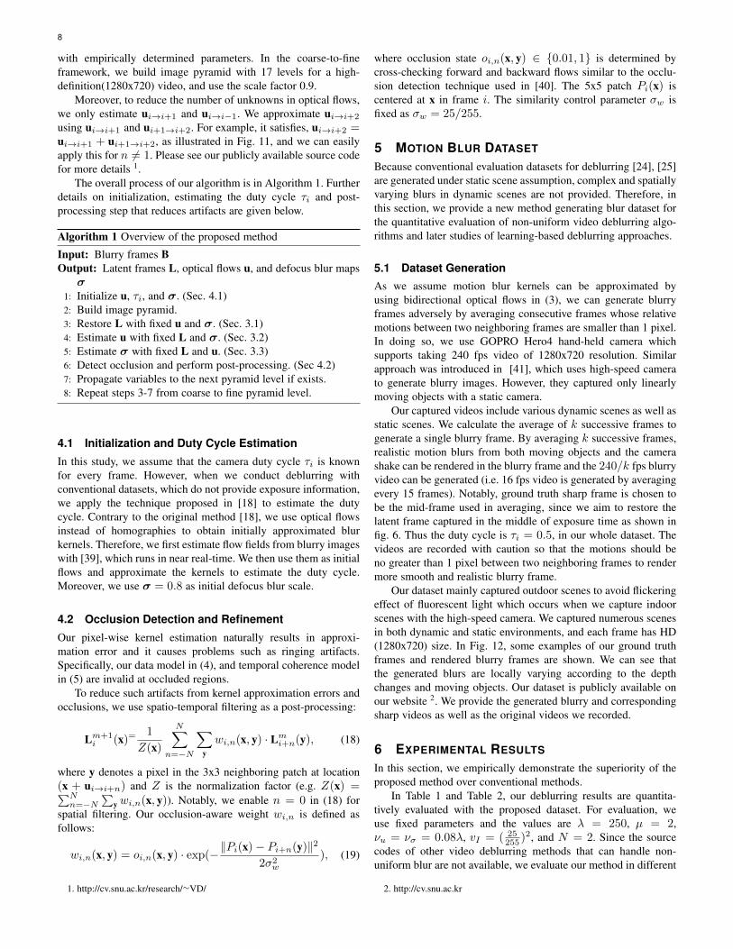
Fig. 10: (a) Real blurry frame. (b) Our jointly estimated latentframe. (c) Color coded optical flow from [30]. (d) Our opticalflow.

as brightness constancy and gradient constancy can not be utilizeddirectly, since such constraints do not hold between two blurryframes. A blur-aware optical flow estimation method from blurryimages has been proposed by Portz et al. [30]. This method isbased on the commutative law of shift-invariant kernels suchthat the brightness of the corresponding points is constant afterconvolving the blur kernel of each image with the other image.However, the commutative law does not hold when the motionis not translational and when the blur kernels vary spatially.Therefore, this approach only works when the motion is verysmooth.

To address this problem, we propose a new model that es-timates optical flow between two latent sharp frames to enableabrupt changes in motions and the blur kernels. In using thismodel, we need not restrict our motion blur kernels to be shiftinvariant. Our model is based on the conventional optical flowconstraint between latent frames, that is, brightness constancy. Theformulation of this model is given by,

Etemporal(L, u) =

µ∑i

∑x

N∑n=−N

|Li(x)− Li+n(x + ui→i+n)|,(5)

where n denotes the index of neighboring frames at i, and theparameter µ controls the weight. We apply the robust L1 norm forrobustness against outliers and occlusions.

Notably, a major difference between the proposed model andthe conventional optical flow estimation methods is that ourproblem is a joint problem. That is, the latent frames and opticalflows should be solved simultaneously. Therefore, the proposedmodel in (5) estimates the latent frames which are temporallycoherent among neighboring frames, and optical flows betweenneighboring frames, simultaneously. Therefore we can estimateaccurate flows at the motion boundaries as shown in Fig. 10.Notice that, our flows at the motion boundaries of moving caris much clearer in comparison with the blur-aware flow estimationmethod by [30].

2.3 Spatial RegularizationTo alleviate the difficulties of highly ill-posed deblurring, opticalflow estimation, and defocus blur map estimation problems, it is

important to adopt spatial regularizers. In doing so, we enforcespatial coherence to penalize spatial fluctuations while allowingdiscontinuities in latent frames, flow fields, and defocus blur maps.With the assumption that spatial priors for the latent frames,optical flows, and defocus blur maps are independent, we canformulate the spatial regularization as follows:

Espatial(L, u) =∑i

|∇Li|+ νσ∑i

∑xgi(x)|∇σi|+

νu∑i

∑x

N∑n=−N

gi(x)|∇ui→i+n|),(6)

wherer parameters νσ and νu control the weights of the secondand third terms.

The first term in (6) denotes the spatial regularization term forthe latent frames. Although more sparse Lp norms (e.g. p = 0.8)fit the gradient statistics of natural sharp images better [32], [33],[34], we use conventional total variation (TV) based regulariza-tion [16], [35], [36], as TV is computationally less expensiveand easy to minimize. The second and third terms enforce spatialsmoothness for defocus blur maps and optical flows, respectively.These regularizers are also based on TV regularization, andcoupled with edge-map to preserve discontinuities at the edgesin both vector fields. Similar to the edge-map used in conventionaloptical flow estimation method [37], our edge-map is expressed asfollows:

gi(x) = exp(−( |∇Li,0|2

vI)), (7)

where the fixed parameter vI controls the weight of the edge-map,and Li,0 is an initial latent image in the iterative optimizationframework.

3 OPTIMIZATION FRAMEWORK

Under the condition that the camera duty cycle τi is known, bycombining Edata, Etemporal, and Espatial, we can have the finalobjective function as follows: and the final objective function whencamera duty cycle τi is known becomes as follows:

minL,u,σ

λ∑i

∑∂∗

‖∂∗Ki(ui→i+1, ui→i−1)Gi(σi)Li − ∂∗Bi‖2+

µ∑i

∑x

N∑n=−N

|Li(x)− Li+n(x + ui→i+n)|+∑i

|∇Li|+ νσ∑i

∑xgi(x)|∇σi|+

νu∑i

∑x

N∑n=−N

gi(x)|∇ui→i+n|).

(8)

Note that contrast with Cho et al. [18] that performs multipleapproaches sequentially, our model finds a solution by minimizingthe proposed single objective function in (8). However, becauseof its non-convexity, our model needs to adopt a practical opti-mization method to obtain an approximated solution. Therefore,we divide the original problem into several simple sub-problemsand then use conventional iterative and alternating optimizationtechniques [1], [15], [16] to minimize the original non-convexobjective function. In the following sections, we introduce efficientsolvers and describe how to estimate unknowns L, u and σalternatively.

KIM et al.: DYNAMIC SCENE DEBLURRING USING A LOCALLY ADAPTIVE LINEAR BLUR MODEL 7

3.1 Sharp Video Restoration

If the motion blur kernels K and the defocus blur kernels G arefixed, then the objective function in (8) becomes convex withrespect to L, and it can be reformulated as follows:

minL

λ∑i

∑∂∗

‖∂∗KiGiLi − ∂∗Bi‖2 +∑i

|∇Li|+

µ∑i

∑x

N∑n=−N

|Li(x)− Li+n(x + ui→i+n)|.(9)

To restore the latent frames L, we adopt the conventional convexoptimization method proposed in [38], and derive the primal-dualupdate scheme as follows:

sm+1 = sm+ηLALm

max(1, abs(sm+ηLALm))

qm+1 = qm+ηLµDLm

max(1, abs(qm+ηLµDLm))

Lm+1 = arg minLm+1

λ∑i

∑∂∗

‖∂∗KiGiLm+1i − ∂∗Bi‖2+

‖Lm+1 − (Lm − εL(AT sm+1 + µDTqm+1))‖2

2εL,

(10)where m ≥ 0 indicates the iteration number, and, sm and qmdenote the dual variables of the concatenated latent frames Lm.Parameters ηL and εL denote the update steps. Linear operator Acalculates the spatial difference between neighboring pixels, andoperator D calculates the temporal differences among neighboringframes using fixed optical flows. The last formulation in (10) is toupdate and optimize the primal variable Lm+1, and we apply theconjugate gradient method to minimize it since it is a quadraticfunction.

3.2 Optical Flows Estimation

Note that , although the latent frames L and the defocus blurkernels G are fixed, the temporal coherence term Etemporal andthe data term Edata are still non-convex. So, let us denote thosetwo terms as a non-convex function ρu(.) as follows:

ρu(u) = µ∑i

∑x

N∑n=−N

|Li(x)− Li+n(x + ui→i+n)|+

λ∑i

∑∂∗

‖∂∗Ki(ui→i+1, ui→i−1)GiLi − ∂∗Bi‖2.(11)

To find the optimal optical flows u, we first convexify the non-convex function ρu(.) by applying the first-order Taylor expan-sion. Similar to the technique in [16], we linearize the functionnear an initial u0 in the iterative process as follows:

ρu(u) ≈ ρu(u0) +∇ρu(u0)T (u− u0). (12)

In doing so, (8) can be approximated by a convex function w.r.t uas follows:

minuρu(u0)+∇ρu(u0)

T (u− u0)+

νu∑i

∑x

N∑n=−N

gi(x)|∇ui→i+n|.(13)

𝐋𝑖 𝐋𝑖+1 𝐋𝑖+2

𝐱 𝐱 + 𝐮𝒊→𝒊+𝟏

𝐱 + 𝐮𝒊→𝒊+𝟏+ 𝐮𝒊+𝟏→𝒊+𝟐

Fig. 11: Temporally consistent optical flows over three frames.

Now, we can apply the convex optimization technique in [38]to the approximated convex function, and the primal-dual updateprocess is expressed as follows:

pm+1 = pm+ηu(νuWuAu)um

max(1, abs(pm+ηu(νuWuAu)um))

um+1 = (um − εu(νuWuAu)Tpm+1)− εu∇ρu(u0),(14)

where p denotes the dual variable of u on the vector space. Weight-ing matrix Wu is diagonal, and its sub-matrix associated withui→i+n is defined as diag(gi(x)). Linear operator Au calculatesthe spatial difference between four nearest neighboring pixels, andparameters ηu and εu denote the update steps.

3.3 Defocus Blur Map EstimationWhen the latent frames L and the motion blur kernels K are fixed,we can estimate the defocus blur maps from (8). However, thedata term is non-convex, and thus an approximation technique isrequired to optimize the objective function. Similar to our opticalflows estimation technique, we approximate and convexify theoriginal function using linearization.

First, we define a non-convex data function ρσ(.), and approx-imate it near an initial values σ0 as follows:

ρσ(σ) = λ∑i

∑∂∗

‖∂∗KiGi(σi)Li − ∂∗Bi‖2

≈ ρσ(σ0) +∇ρσ(σ0)T (σ − σ0),

(15)

and the approximated convex function for defocus blur mapestimation is given by,

minσ

ρσ(σ0)+∇ρσ(σ0)T (σ − σ0)+

νσ∑i

∑xgi(x)|∇σi|.

(16)

Similarly, (16) can be optimized using [38], and the primal-dual update formulation is given by,

rm+1 = rm+ησ(νσWσA)σm

max(1, abs(rm+ησ(νσWσA)σm))

σm+1 = (σm − εσ(νσWσA)T rm+1)− εσ∇ρσ(σ0),(17)

where r denotes the dual variable of σ on the vector field.Weighting matrix Wσ is diagonal, and its sub-matrix associatedwith σi is defined as diag(gi(x)). Parameters ησ and εσ denotethe update steps.

4 IMPLEMENTATION DETAILS

To handle large blurs and guide fast convergence, we imple-ment our algorithm on the conventional coarse-to-fine framework

8

with empirically determined parameters. In the coarse-to-fineframework, we build image pyramid with 17 levels for a high-definition(1280x720) video, and use the scale factor 0.9.

Moreover, to reduce the number of unknowns in optical flows,we only estimate ui→i+1 and ui→i−1. We approximate ui→i+2

using ui→i+1 and ui+1→i+2. For example, it satisfies, ui→i+2 =ui→i+1 + ui+1→i+2, as illustrated in Fig. 11, and we can easilyapply this for n 6= 1. Please see our publicly available source codefor more details 1.

The overall process of our algorithm is in Algorithm 1. Furtherdetails on initialization, estimating the duty cycle τi and post-processing step that reduces artifacts are given below.

Algorithm 1 Overview of the proposed method

Input: Blurry frames BOutput: Latent frames L, optical flows u, and defocus blur maps

σ1: Initialize u, τi, and σ. (Sec. 4.1)2: Build image pyramid.3: Restore L with fixed u and σ. (Sec. 3.1)4: Estimate u with fixed L and σ. (Sec. 3.2)5: Estimate σ with fixed L and u. (Sec. 3.3)6: Detect occlusion and perform post-processing. (Sec 4.2)7: Propagate variables to the next pyramid level if exists.8: Repeat steps 3-7 from coarse to fine pyramid level.

4.1 Initialization and Duty Cycle Estimation

In this study, we assume that the camera duty cycle τi is knownfor every frame. However, when we conduct deblurring withconventional datasets, which do not provide exposure information,we apply the technique proposed in [18] to estimate the dutycycle. Contrary to the original method [18], we use optical flowsinstead of homographies to obtain initially approximated blurkernels. Therefore, we first estimate flow fields from blurry imageswith [39], which runs in near real-time. We then use them as initialflows and approximate the kernels to estimate the duty cycle.Moreover, we use σ = 0.8 as initial defocus blur scale.

4.2 Occlusion Detection and Refinement

Our pixel-wise kernel estimation naturally results in approxi-mation error and it causes problems such as ringing artifacts.Specifically, our data model in (4), and temporal coherence modelin (5) are invalid at occluded regions.

To reduce such artifacts from kernel approximation errors andocclusions, we use spatio-temporal filtering as a post-processing:

Lm+1i (x)=

1

Z(x)

N∑n=−N

∑ywi,n(x, y) · Lmi+n(y), (18)

where y denotes a pixel in the 3x3 neighboring patch at location(x + ui→i+n) and Z is the normalization factor (e.g. Z(x) =∑Nn=−N

∑y wi,n(x, y)). Notably, we enable n = 0 in (18) for

spatial filtering. Our occlusion-aware weight wi,n is defined asfollows:

wi,n(x, y) = oi,n(x, y) · exp(−‖Pi(x)− Pi+n(y)‖2

2σ2w

), (19)

1. http://cv.snu.ac.kr/research/∼VD/

where occlusion state oi,n(x, y) ∈ {0.01, 1} is determined bycross-checking forward and backward flows similar to the occlu-sion detection technique used in [40]. The 5x5 patch Pi(x) iscentered at x in frame i. The similarity control parameter σw isfixed as σw = 25/255.

5 MOTION BLUR DATASET

Because conventional evaluation datasets for deblurring [24], [25]are generated under static scene assumption, complex and spatiallyvarying blurs in dynamic scenes are not provided. Therefore, inthis section, we provide a new method generating blur dataset forthe quantitative evaluation of non-uniform video deblurring algo-rithms and later studies of learning-based deblurring approaches.

5.1 Dataset GenerationAs we assume motion blur kernels can be approximated byusing bidirectional optical flows in (3), we can generate blurryframes adversely by averaging consecutive frames whose relativemotions between two neighboring frames are smaller than 1 pixel.In doing so, we use GOPRO Hero4 hand-held camera whichsupports taking 240 fps video of 1280x720 resolution. Similarapproach was introduced in [41], which uses high-speed camerato generate blurry images. However, they captured only linearlymoving objects with a static camera.

Our captured videos include various dynamic scenes as well asstatic scenes. We calculate the average of k successive frames togenerate a single blurry frame. By averaging k successive frames,realistic motion blurs from both moving objects and the camerashake can be rendered in the blurry frame and the 240/k fps blurryvideo can be generated (i.e. 16 fps video is generated by averagingevery 15 frames). Notably, ground truth sharp frame is chosen tobe the mid-frame used in averaging, since we aim to restore thelatent frame captured in the middle of exposure time as shown infig. 6. Thus the duty cycle is τi = 0.5, in our whole dataset. Thevideos are recorded with caution so that the motions should beno greater than 1 pixel between two neighboring frames to rendermore smooth and realistic blurry frame.

Our dataset mainly captured outdoor scenes to avoid flickeringeffect of fluorescent light which occurs when we capture indoorscenes with the high-speed camera. We captured numerous scenesin both dynamic and static environments, and each frame has HD(1280x720) size. In Fig. 12, some examples of our ground truthframes and rendered blurry frames are shown. We can see thatthe generated blurs are locally varying according to the depthchanges and moving objects. Our dataset is publicly available onour website 2. We provide the generated blurry and correspondingsharp videos as well as the original videos we recorded.

6 EXPERIMENTAL RESULTS

In this section, we empirically demonstrate the superiority of theproposed method over conventional methods.

In Table 1 and Table 2, our deblurring results are quantita-tively evaluated with the proposed dataset. For evaluation, weuse fixed parameters and the values are λ = 250, µ = 2,νu = νσ = 0.08λ, vI = ( 25

255 )2, and N = 2. Since the source

codes of other video deblurring methods that can handle non-uniform blur are not available, we evaluate our method in different

2. http://cv.snu.ac.kr

KIM et al.: DYNAMIC SCENE DEBLURRING USING A LOCALLY ADAPTIVE LINEAR BLUR MODEL 9

(a) (b)

Fig. 12: (a) Ground truth sharp frames. (b) Generated blurry frames. Spatially varying blurs by object motions and camera shakes aresynthesized realistically.

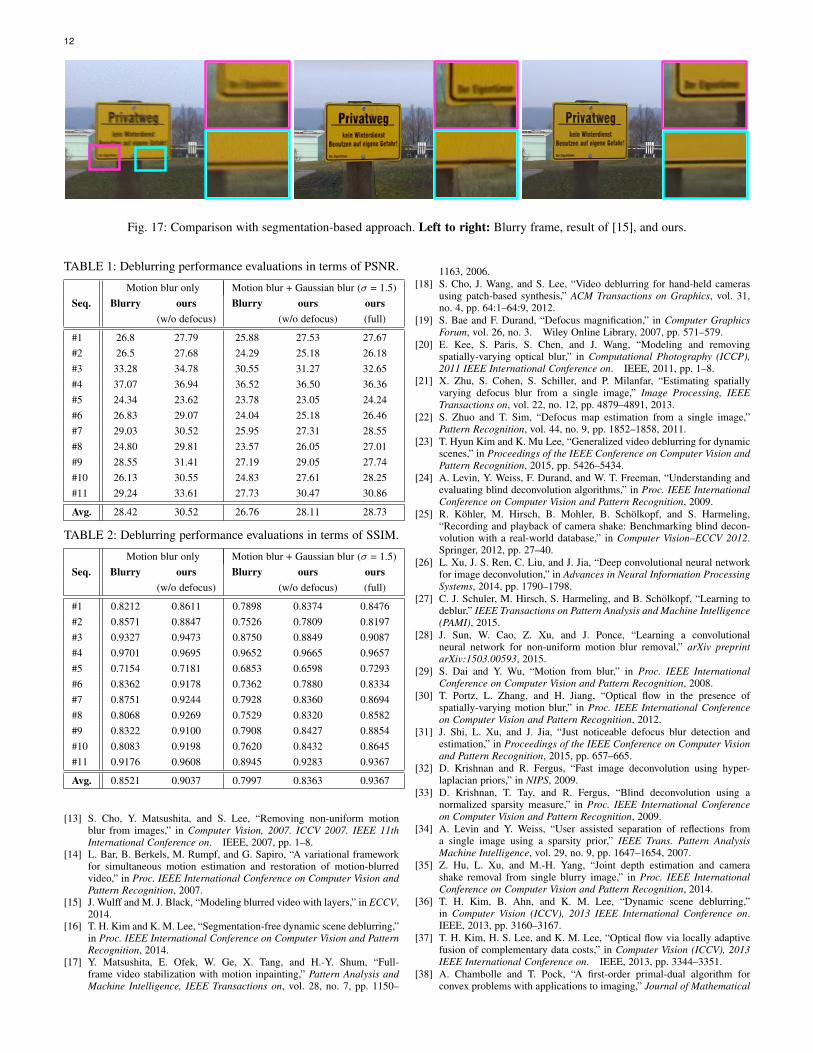
settings. First, we calculate and compare both the PSNR and SSIMvalues of each original blurry sequence and the correspondingdeblurred one. As our dataset contains only motion blurs in it,we restore the latent frames without considering the defocusblur (defocus blur kernel is set to be identity matrix). Next, todemonstrate the good performance of the proposed method inremoving defocus blurs, we re-generate blurry dataset by addingGaussian blur (σ = 1.5) to the original sharp video beforeaveraging. Using this dataset which contains both motion blurand defocus blur, we compare the our result against each originalblurry sequence and our deblurring result that does not considerdefocus blur. We verify that, our approach improves the deblurringresults significantly in terms of PSNR and SSIM by removingblurs from defocus. In Fig. 13, qualitative comparisons using ourdataset are shown. Ours restores the edges of buildings, letters,and moving persons, clearly. However, we observe some failurecases in our results. In Fig. 14, we fail to estimate motions of fastmoving hand, and thus fail in deblurring, since it is difficult toestimate accurate flows of small structure with distinct motions inthe coarse-to-fine framework as reported in [42].

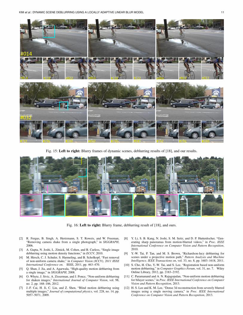
Next, we compare our deblurring results with those of thestate-of-the art exemplar based method [18] with the videosused in [18]. As shown in Fig. 15, the captured scenes aredynamic and contain multiple moving objects. The method [18]fails in restoring the moving objects, because the object motionsare large and distinct from the backgrounds. By contrast, ourresults show better performances in deblurring moving objects andbackgrounds. Notably, the exemplar-based approach also fails inhandling large blurs, as shown in Fig. 16, as the initially esti-

(a) (b)

Fig. 14: A failure case. (a) A blurry frame in the proposed dataset.(b) Our deblurring result.

mated homographies in the largely blurred images are inaccurate.Moreover, this approach renders excessively smooth results formid-frequency textures such as trees, as the method is based oninterpolation without spatial prior for latent frames.

We also compare our method with the state-of-the-artsegmentation-based approach [15]. The test video is shown inFig. 17, which is a bilayer scene used in [15]. Although thebi-layer scene is a good example to verify the performance ofthe layered model, inaccurate segmentation near the boundariescauses serious artifacts in the restored frame. By contrast, sinceour method does not need segmentation and it restores the bound-aries much better than the layered model.

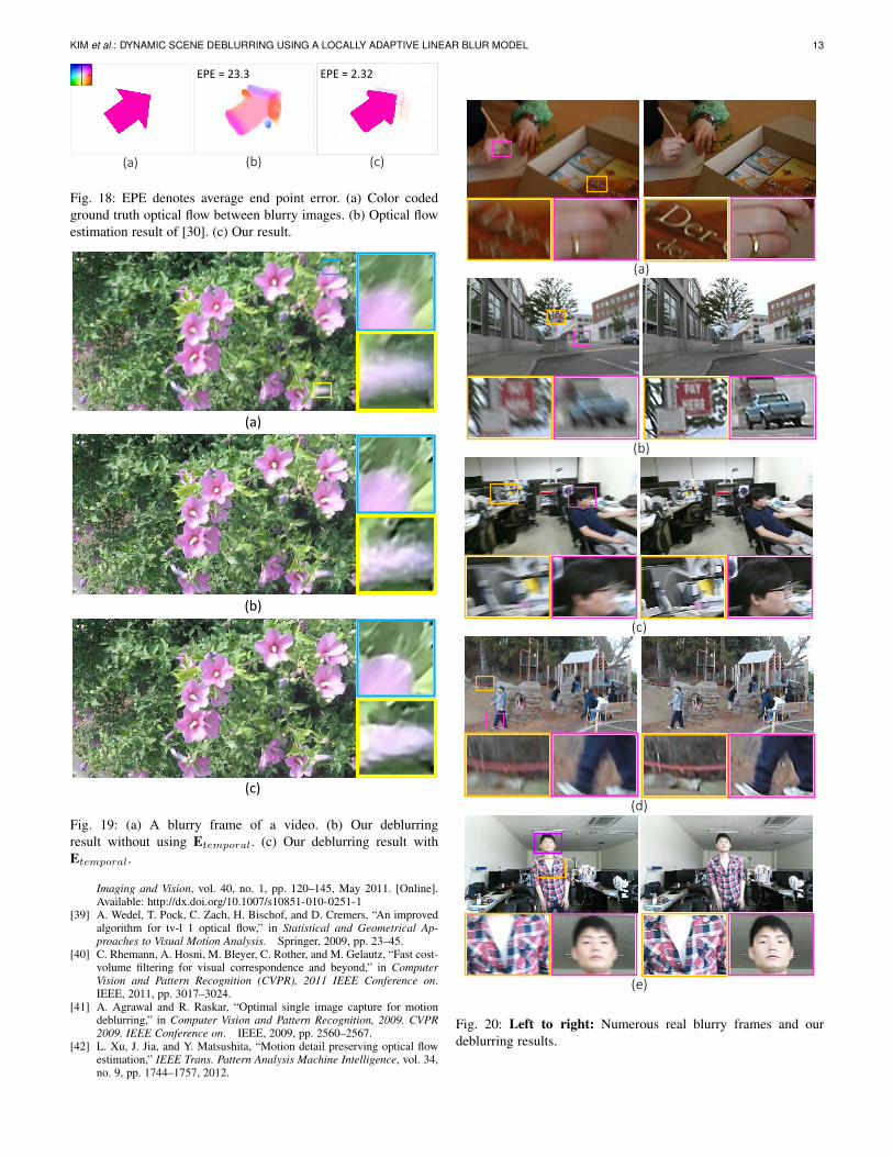
In Fig. 18, we quantitatively compare the optical flow accu-racies with [30] on synthetic blurry images. As publicly availablecode of [30] cannot handle Gaussian blur, we synthesize blurryframes which have motion blurs only. Although [30] was proposedto handle blurry images in optical flow estimation, its assumptiondoes not hold in motion boundaries, which is very important for

10

(a) (b) (c) (d)

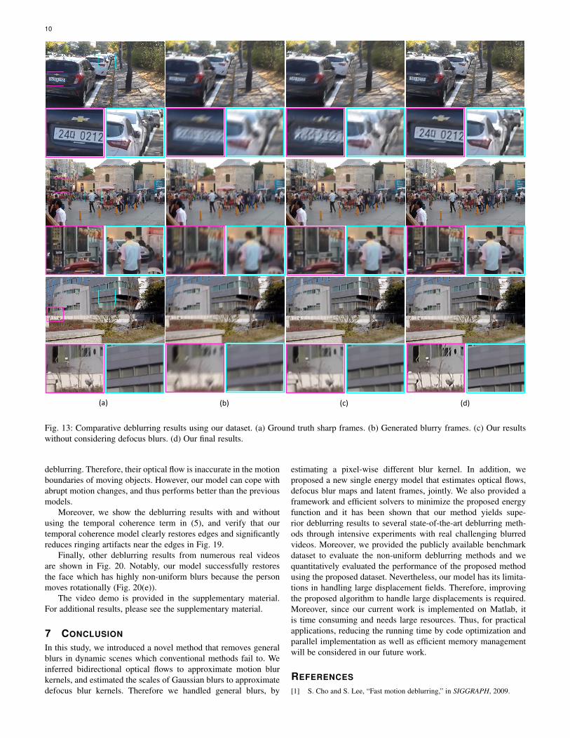
Fig. 13: Comparative deblurring results using our dataset. (a) Ground truth sharp frames. (b) Generated blurry frames. (c) Our resultswithout considering defocus blurs. (d) Our final results.

deblurring. Therefore, their optical flow is inaccurate in the motionboundaries of moving objects. However, our model can cope withabrupt motion changes, and thus performs better than the previousmodels.

Moreover, we show the deblurring results with and withoutusing the temporal coherence term in (5), and verify that ourtemporal coherence model clearly restores edges and significantlyreduces ringing artifacts near the edges in Fig. 19.

Finally, other deblurring results from numerous real videosare shown in Fig. 20. Notably, our model successfully restoresthe face which has highly non-uniform blurs because the personmoves rotationally (Fig. 20(e)).

The video demo is provided in the supplementary material.For additional results, please see the supplementary material.

7 CONCLUSION

In this study, we introduced a novel method that removes generalblurs in dynamic scenes which conventional methods fail to. Weinferred bidirectional optical flows to approximate motion blurkernels, and estimated the scales of Gaussian blurs to approximatedefocus blur kernels. Therefore we handled general blurs, by

estimating a pixel-wise different blur kernel. In addition, weproposed a new single energy model that estimates optical flows,defocus blur maps and latent frames, jointly. We also provided aframework and efficient solvers to minimize the proposed energyfunction and it has been shown that our method yields supe-rior deblurring results to several state-of-the-art deblurring meth-ods through intensive experiments with real challenging blurredvideos. Moreover, we provided the publicly available benchmarkdataset to evaluate the non-uniform deblurring methods and wequantitatively evaluated the performance of the proposed methodusing the proposed dataset. Nevertheless, our model has its limita-tions in handling large displacement fields. Therefore, improvingthe proposed algorithm to handle large displacements is required.Moreover, since our current work is implemented on Matlab, itis time consuming and needs large resources. Thus, for practicalapplications, reducing the running time by code optimization andparallel implementation as well as efficient memory managementwill be considered in our future work.

REFERENCES

[1] S. Cho and S. Lee, “Fast motion deblurring,” in SIGGRAPH, 2009.

KIM et al.: DYNAMIC SCENE DEBLURRING USING A LOCALLY ADAPTIVE LINEAR BLUR MODEL 11

#032

#032

#036 #040 #032 #036 #040 #032 #036 #040

#014 #018 #022 #014 #018 #022 #014 #018 #022

#014

Fig. 15: Left to right: Blurry frames of dynamic scenes, deblurring results of [18], and our results.

Fig. 16: Left to right: Blurry frame, deblurring result of [18], and ours.

[2] R. Fergus, B. Singh, A. Hertzmann, S. T. Roweis, and W. Freeman,“Removing camera shake from a single photograph,” in SIGGRAPH,2006.

[3] A. Gupta, N. Joshi, L. Zitnick, M. Cohen, and B. Curless, “Single imagedeblurring using motion density functions,” in ECCV, 2010.

[4] M. Hirsch, C. J. Schuler, S. Harmeling, and B. Scholkopf, “Fast removalof non-uniform camera shake,” in Computer Vision (ICCV), 2011 IEEEInternational Conference on. IEEE, 2011, pp. 463–470.

[5] Q. Shan, J. Jia, and A. Agarwala, “High-quality motion deblurring froma single image,” in SIGGRAPH, 2008.

[6] O. Whyte, J. Sivic, A. Zisserman, and J. Ponce, “Non-uniform deblurringfor shaken images,” International Journal of Computer Vision, vol. 98,no. 2, pp. 168–186, 2012.

[7] J.-F. Cai, H. Ji, C. Liu, and Z. Shen, “Blind motion deblurring usingmultiple images,” Journal of computational physics, vol. 228, no. 14, pp.5057–5071, 2009.

[8] Y. Li, S. B. Kang, N. Joshi, S. M. Seitz, and D. P. Huttenlocher, “Gen-erating sharp panoramas from motion-blurred videos,” in Proc. IEEEInternational Conference on Computer Vision and Pattern Recognition,2010.

[9] Y.-W. Tai, P. Tan, and M. S. Brown, “Richardson-lucy deblurring forscenes under a projective motion path,” Pattern Analysis and MachineIntelligence, IEEE Transactions on, vol. 33, no. 8, pp. 1603–1618, 2011.

[10] S. Cho, H. Cho, Y.-W. Tai, and S. Lee, “Registration based non-uniformmotion deblurring,” in Computer Graphics Forum, vol. 31, no. 7. WileyOnline Library, 2012, pp. 2183–2192.

[11] C. Paramanand and A. N. Rajagopalan, “Non-uniform motion deblurringfor bilayer scenes,” in Proc. IEEE International Conference on ComputerVision and Pattern Recognition, 2013.

[12] H. S. Lee and K. M. Lee, “Dense 3d reconstruction from severely blurredimages using a single moving camera,” in Proc. IEEE InternationalConference on Computer Vision and Pattern Recognition, 2013.

12

Fig. 17: Comparison with segmentation-based approach. Left to right: Blurry frame, result of [15], and ours.

TABLE 1: Deblurring performance evaluations in terms of PSNR.

Motion blur only Motion blur + Gaussian blur (σ = 1.5)Seq. Blurry ours Blurry ours ours

(w/o defocus) (w/o defocus) (full)

#1 26.8 27.79 25.88 27.53 27.67#2 26.5 27.68 24.29 25.18 26.18#3 33.28 34.78 30.55 31.27 32.65#4 37.07 36.94 36.52 36.50 36.36#5 24.34 23.62 23.78 23.05 24.24#6 26.83 29.07 24.04 25.18 26.46#7 29.03 30.52 25.95 27.31 28.55#8 24.80 29.81 23.57 26.05 27.01#9 28.55 31.41 27.19 29.05 27.74#10 26.13 30.55 24.83 27.61 28.25#11 29.24 33.61 27.73 30.47 30.86

Avg. 28.42 30.52 26.76 28.11 28.73

TABLE 2: Deblurring performance evaluations in terms of SSIM.

Motion blur only Motion blur + Gaussian blur (σ = 1.5)Seq. Blurry ours Blurry ours ours

(w/o defocus) (w/o defocus) (full)

#1 0.8212 0.8611 0.7898 0.8374 0.8476#2 0.8571 0.8847 0.7526 0.7809 0.8197#3 0.9327 0.9473 0.8750 0.8849 0.9087#4 0.9701 0.9695 0.9652 0.9665 0.9657#5 0.7154 0.7181 0.6853 0.6598 0.7293#6 0.8362 0.9178 0.7362 0.7880 0.8334#7 0.8751 0.9244 0.7928 0.8360 0.8694#8 0.8068 0.9269 0.7529 0.8320 0.8582#9 0.8322 0.9100 0.7908 0.8427 0.8854#10 0.8083 0.9198 0.7620 0.8432 0.8645#11 0.9176 0.9608 0.8945 0.9283 0.9367

Avg. 0.8521 0.9037 0.7997 0.8363 0.9367

[13] S. Cho, Y. Matsushita, and S. Lee, “Removing non-uniform motionblur from images,” in Computer Vision, 2007. ICCV 2007. IEEE 11thInternational Conference on. IEEE, 2007, pp. 1–8.

[14] L. Bar, B. Berkels, M. Rumpf, and G. Sapiro, “A variational frameworkfor simultaneous motion estimation and restoration of motion-blurredvideo,” in Proc. IEEE International Conference on Computer Vision andPattern Recognition, 2007.

[15] J. Wulff and M. J. Black, “Modeling blurred video with layers,” in ECCV,2014.

[16] T. H. Kim and K. M. Lee, “Segmentation-free dynamic scene deblurring,”in Proc. IEEE International Conference on Computer Vision and PatternRecognition, 2014.

[17] Y. Matsushita, E. Ofek, W. Ge, X. Tang, and H.-Y. Shum, “Full-frame video stabilization with motion inpainting,” Pattern Analysis andMachine Intelligence, IEEE Transactions on, vol. 28, no. 7, pp. 1150–

1163, 2006.[18] S. Cho, J. Wang, and S. Lee, “Video deblurring for hand-held cameras

using patch-based synthesis,” ACM Transactions on Graphics, vol. 31,no. 4, pp. 64:1–64:9, 2012.

[19] S. Bae and F. Durand, “Defocus magnification,” in Computer GraphicsForum, vol. 26, no. 3. Wiley Online Library, 2007, pp. 571–579.

[20] E. Kee, S. Paris, S. Chen, and J. Wang, “Modeling and removingspatially-varying optical blur,” in Computational Photography (ICCP),2011 IEEE International Conference on. IEEE, 2011, pp. 1–8.

[21] X. Zhu, S. Cohen, S. Schiller, and P. Milanfar, “Estimating spatiallyvarying defocus blur from a single image,” Image Processing, IEEETransactions on, vol. 22, no. 12, pp. 4879–4891, 2013.

[22] S. Zhuo and T. Sim, “Defocus map estimation from a single image,”Pattern Recognition, vol. 44, no. 9, pp. 1852–1858, 2011.

[23] T. Hyun Kim and K. Mu Lee, “Generalized video deblurring for dynamicscenes,” in Proceedings of the IEEE Conference on Computer Vision andPattern Recognition, 2015, pp. 5426–5434.

[24] A. Levin, Y. Weiss, F. Durand, and W. T. Freeman, “Understanding andevaluating blind deconvolution algorithms,” in Proc. IEEE InternationalConference on Computer Vision and Pattern Recognition, 2009.

[25] R. Kohler, M. Hirsch, B. Mohler, B. Scholkopf, and S. Harmeling,“Recording and playback of camera shake: Benchmarking blind decon-volution with a real-world database,” in Computer Vision–ECCV 2012.Springer, 2012, pp. 27–40.

[26] L. Xu, J. S. Ren, C. Liu, and J. Jia, “Deep convolutional neural networkfor image deconvolution,” in Advances in Neural Information ProcessingSystems, 2014, pp. 1790–1798.

[27] C. J. Schuler, M. Hirsch, S. Harmeling, and B. Scholkopf, “Learning todeblur,” IEEE Transactions on Pattern Analysis and Machine Intelligence(PAMI), 2015.

[28] J. Sun, W. Cao, Z. Xu, and J. Ponce, “Learning a convolutionalneural network for non-uniform motion blur removal,” arXiv preprintarXiv:1503.00593, 2015.

[29] S. Dai and Y. Wu, “Motion from blur,” in Proc. IEEE InternationalConference on Computer Vision and Pattern Recognition, 2008.

[30] T. Portz, L. Zhang, and H. Jiang, “Optical flow in the presence ofspatially-varying motion blur,” in Proc. IEEE International Conferenceon Computer Vision and Pattern Recognition, 2012.

[31] J. Shi, L. Xu, and J. Jia, “Just noticeable defocus blur detection andestimation,” in Proceedings of the IEEE Conference on Computer Visionand Pattern Recognition, 2015, pp. 657–665.

[32] D. Krishnan and R. Fergus, “Fast image deconvolution using hyper-laplacian priors,” in NIPS, 2009.

[33] D. Krishnan, T. Tay, and R. Fergus, “Blind deconvolution using anormalized sparsity measure,” in Proc. IEEE International Conferenceon Computer Vision and Pattern Recognition, 2009.

[34] A. Levin and Y. Weiss, “User assisted separation of reflections froma single image using a sparsity prior,” IEEE Trans. Pattern AnalysisMachine Intelligence, vol. 29, no. 9, pp. 1647–1654, 2007.

[35] Z. Hu, L. Xu, and M.-H. Yang, “Joint depth estimation and camerashake removal from single blurry image,” in Proc. IEEE InternationalConference on Computer Vision and Pattern Recognition, 2014.

[36] T. H. Kim, B. Ahn, and K. M. Lee, “Dynamic scene deblurring,”in Computer Vision (ICCV), 2013 IEEE International Conference on.IEEE, 2013, pp. 3160–3167.

[37] T. H. Kim, H. S. Lee, and K. M. Lee, “Optical flow via locally adaptivefusion of complementary data costs,” in Computer Vision (ICCV), 2013IEEE International Conference on. IEEE, 2013, pp. 3344–3351.

[38] A. Chambolle and T. Pock, “A first-order primal-dual algorithm forconvex problems with applications to imaging,” Journal of Mathematical

KIM et al.: DYNAMIC SCENE DEBLURRING USING A LOCALLY ADAPTIVE LINEAR BLUR MODEL 13

(b) (c)

EPE = 23.3 EPE = 2.32

(a)

Fig. 18: EPE denotes average end point error. (a) Color codedground truth optical flow between blurry images. (b) Optical flowestimation result of [30]. (c) Our result.

(a)

(b)

(c)

(a)

(b)

(c)

Fig. 19: (a) A blurry frame of a video. (b) Our deblurringresult without using Etemporal. (c) Our deblurring result withEtemporal.

Imaging and Vision, vol. 40, no. 1, pp. 120–145, May 2011. [Online].Available: http://dx.doi.org/10.1007/s10851-010-0251-1

[39] A. Wedel, T. Pock, C. Zach, H. Bischof, and D. Cremers, “An improvedalgorithm for tv-l 1 optical flow,” in Statistical and Geometrical Ap-proaches to Visual Motion Analysis. Springer, 2009, pp. 23–45.

[40] C. Rhemann, A. Hosni, M. Bleyer, C. Rother, and M. Gelautz, “Fast cost-volume filtering for visual correspondence and beyond,” in ComputerVision and Pattern Recognition (CVPR), 2011 IEEE Conference on.IEEE, 2011, pp. 3017–3024.

[41] A. Agrawal and R. Raskar, “Optimal single image capture for motiondeblurring,” in Computer Vision and Pattern Recognition, 2009. CVPR2009. IEEE Conference on. IEEE, 2009, pp. 2560–2567.

[42] L. Xu, J. Jia, and Y. Matsushita, “Motion detail preserving optical flowestimation,” IEEE Trans. Pattern Analysis Machine Intelligence, vol. 34,no. 9, pp. 1744–1757, 2012.

(c)

(d)

(e)

(a)

(b)

Fig. 20: Left to right: Numerous real blurry frames and ourdeblurring results.

14

Tae Hyun Kim received the BS degree and theMS degree in the department of electrical en-gineering from KAIST, Daejeon, Korea, in 2008and 2010, respectively. He is currently workingtoward the PhD degree in Electrical and Com-puter Engineering at Seoul National University.His research interests include motion estimation,and deblurring. He is a student member of theIEEE.

Seungjun Nah received the BS degree in Elec-trical and Computer Engineering from Seoul Na-tional University (SNU), Seoul, Korea in 2014.He is currently working towards PhD degree inElectrical and Computer Engineering at SeoulNational University. He is interested in computervision problems including deblurring and visualsaliency. He is a student member of the IEEE.

Kyoung Mu Lee received the BS and MS de-grees in control and instrumentation engineeringfrom Seoul National University (SNU), Seoul,Korea in 1984 and 1986, respectively, and thePhD degree in electrical engineering from theUniversity of Southern California (USC), Los An-geles, California in 1993. He received the Ko-rean Government Overseas Scholarship duringthe PhD courses. From 1993 to 1994, he wasa research associate in the Signal and ImageProcessing Institute (SIPI) at USC. He was with

the Samsung Electronics Co. Ltd. in Korea as a senior researcherfrom 1994 to 1995. In August 1995, he joined the Department of Elec-tronics and Electrical Engineering of the Hong-Ik University, and wasan assistant and associate professor. Since September 2003, he hasbeen with the Department of Electrical and Computer Engineering atSeoul National University as a professor, and leads the Computer VisionLaboratory. His primary research is focused on statistical methods incomputer vision that can be applied to various applications includingobject recognition, segmentation, tracking and 3D reconstruction. Hehas received several awards, in particular, the Most Influential Paperover the Decade Award by the IAPR Machine Vision Application in 2009,the ACCV Honorable Mention Award in 2007, the Okawa FoundationResearch Grant Award in 2006, and the Outstanding Research Award bythe College of Engineering of SNU in 2010. He served as an AssociateEditor in Chief, Editorial Board member of the EURASIP Journal ofApplied Signal Processing, and is an associate editor of the MachineVision Application Journal, the IPSJ Transactions on Computer Visionand Applications, and the Journal of Information Hiding and MultimediaSignal Processing. He has (co)authored more than 100 publications inrefereed journals and conferences including PAMI, IJCV, CVPR, ICCV,and ECCV.