1

Finding Similar Pairs

Divide-Compute-MergeLocality-Sensitive Hashing

Applications

2

Finding Similar Pairs

Suppose we have in main memory data representing a large number of objects. May be the objects themselves (e.g.,

summaries of faces). May be signatures as in minhashing.

We want to compare each to each, finding those pairs that are sufficiently similar.

3

Candidate Generation From Minhash Signatures

Pick a similarity threshold s, a fraction < 1.

A pair of columns c and d is a candidate pair if their signatures agree in at least fraction s of the rows. I.e., M (i, c ) = M (i, d ) for at least

fraction s values of i.

4

Other Notions of “Sufficiently Similar”

For images, a pair of vectors is a candidate if they differ by at most a small amount t in at least s % of the components.

For entity records, a pair is a candidate if the sum of similarity scores of corresponding components exceeds a threshold.

5

Checking All Pairs is Hard

While the signatures of all columns may fit in main memory, comparing the signatures of all pairs of columns is quadratic in the number of columns.

Example: 106 columns implies 5*1011 comparisons.

At 1 microsecond/comparison: 6 days.

6

Solutions

1. Divide-Compute-Merge (DCM) uses external sorting, merging.

2. Locality-Sensitive Hashing (LSH) can be carried out in main memory, but admits some false negatives.

7

Divide-Compute-Merge

Designed for “shingles” and docs. Or other problems where data is

presented by column. At each stage, divide data into

batches that fit in main memory. Operate on individual batches and

write out partial results to disk. Merge partial results from disk.

8

doc1: s11,s12,…,s1kdoc2: s21,s22,…,s2k…

DCM Steps

s11,doc1s12,doc1…s1k,doc1s21,doc2…

Invertt1,doc11t1,doc12…t2,doc21t2,doc22…

sort onshingleId

doc11,doc12,1doc11,doc13,1…doc21,doc22,1…

Invert and pair

doc11,doc12,1doc11,doc12,1…doc11,doc13,1…

sort on<docId1,docId2>

doc11,doc12,2doc11,doc13,10…

Merge

9

DCM Summary

1. Start with the pairs <shingleId, docId>.2. Sort by shingleId.3. In a sequential scan, generate triplets <docId1,

docId2, 1> for pairs of docs that share a shingle.4. Sort on <docId1, docId2>.5. Merge triplets with common docIds to generate

triplets of the form <docId1,docId2,count>.6. Output document pairs with count > threshold.

10

Some Optimizations

“Invert and Pair” is the most expensive step.

Speed it up by eliminating very common shingles. “the”, “404 not found”, “<A HREF”,

etc. Also, eliminate exact-duplicate

docs first.

11

Locality-Sensitive Hashing

Big idea: hash columns of signature matrix M several times.

Arrange that (only) similar columns are likely to hash to the same bucket.

Candidate pairs are those that hash at least once to the same bucket.

12

Partition Into Bands

Matrix M

r rowsper band

b bands

13

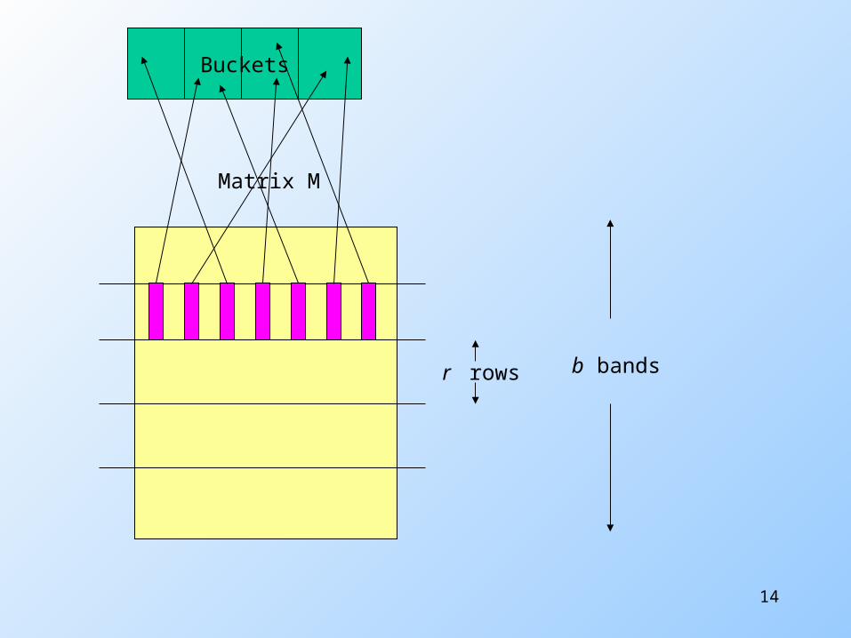
Partition into Bands – (2)

Divide matrix M into b bands of r rows. For each band, hash its portion of each

column to a hash table with k buckets. Candidate column pairs are those that

hash to the same bucket for ≥ 1 band. Tune b and r to catch most similar pairs,

but few nonsimilar pairs.

14

Matrix M

r rows b bands

Buckets

15

Simplifying Assumption

There are enough buckets that columns are unlikely to hash to the same bucket unless they are identical in a particular band.

Hereafter, we assume that “same bucket” means “identical.”

16

Example

Suppose 100,000 columns. Signatures of 100 integers. Therefore, signatures take 40Mb. But 5,000,000,000 pairs of

signatures can take a while to compare.

Choose 20 bands of 5 integers/band.

17

Suppose C1, C2 are 80% Similar

Probability C1, C2 identical in one particular band: (0.8)5 = 0.328.

Probability C1, C2 are not similar in any of the 20 bands: (1-0.328)20 = .00035 . i.e., we miss about 1/3000th of the

80%-similar column pairs.

18

Suppose C1, C2 Only 40% Similar

Probability C1, C2 identical in any one particular band: (0.4)5 = 0.01 .

Probability C1, C2 identical in ≥ 1 of 20 bands: ≤ 20 * 0.01 = 0.2 .

But false positives much lower for similarities << 40%.

19

LSH Involves a Tradeoff

Pick the number of minhashes, the number of bands, and the number of rows per band to balance false positives/negatives.

Example: if we had fewer than 20 bands, the number of false positives would go down, but the number of false negatives would go up.

20

Analysis of LSH – What We Want

Similarity s of two columns

Probabilityof sharinga bucket

t

No chanceif s < t

Probability= 1 if s > t

21

What One Row Gives You

Similarity s of two columns

Probabilityof sharinga bucket

t

Remember:probability ofequal hash-values= similarity

22

What b Bands of r Rows Gives You

Similarity s of two columns

Probabilityof sharinga bucket

t

s r

All rowsof a bandare equal

1 -

Some rowof a bandunequal

( )b

No bandsidentical

1 -

At leastone bandidentical

t ~ (1/b)1/r

23

LSH Summary

Tune to get almost all pairs with similar signatures, but eliminate most pairs that do not have similar signatures.

Check in main memory that candidate pairs really do have similar signatures.

Optional: In another pass through data, check that the remaining candidate pairs really are similar columns .

24

LSH for Other Applications

1. Face recognition from 1000 measurements/face.

2. Entity resolution from name-address-phone records.

General principle: find many hash functions for elements; candidate pairs share a bucket for > 1 hash.

25

Face-Recognition Hash Functions

1. Pick a set of r of the 1000 measurements.

2. Each bucket corresponds to a range of values for each of the r measurements.

3. Hash a vector to the bucket such that each of its r components is in-range.

4. Optional: if near the edge of a range, also hash to an adjacent bucket.

26

Example: r = 2

0-4

5-9

10-14

15-19

38-4431-3724-3017-2310-16

One bucket, for(x,y) if 10<x<16

and 0<y<4

(27,9)goeshere.

Maybeput acopy

here, too.

27

Many-One Face Lookup

As for boolean matrices, use many different hash functions. Each based on a different set of the

1000 measurements. Each bucket of each hash function

points to the images that hash to that bucket.

28

Face Lookup – (2)

Given a new image (the probe ), hash it according to all the hash functions.

Any member of any one of its buckets is a candidate.

For each candidate, count the number of components in which the candidate and probe are close.

Match if #components > threshold.

29

Hashing the Probe

h1 h2 h3 h4 h5

probe

Look in allthese buckets

30

Many-Many Problem

Make each pair of images that are in the same bucket according to any hash function be a candidate pair.

Score each candidate pair as for the many-one problem.

31

Entity Resolution

You don’t have the convenient multidimensional view of data that you do for “face-recognition” or “similar-columns.”

We actually used an LSH-inspired simplification.

32

Matching Customer Records

I once took a consulting job solving the following problem: Company A agreed to solicit customers

for Company B, for a fee. They then had a parting of the ways,

and argued over how many customers. Neither recorded exactly which

customers were involved.

33

Customer Records – (2)

Company B had about 1 million records of all its customers.

Company A had about 1 million records describing customers, some of which it had signed up for B.

Records had name, address, and phone, but for various reasons, they could be different for the same person.

34

Customer Records – (3)

Step 1: design a measure of how similar records are: E.g., deduct points for small

misspellings (“Jeffrey” vs. “Geoffery”), same phone, different area code.

Step 2: score all pairs of records; report very similar records as matches.

35

Customer Records – (4)

Problem: (1 million)2 is too many pairs of records to score.

Solution: A simple LSH. Three hash functions: exact values of

name, address, phone.• Compare iff records are identical in at least

one.

Misses similar records with a small difference in all three fields.

36

Customer Records – Aside

We were able to tell what values of the scoring function were reliable in an interesting way. Identical records had a creation date

difference of 10 days. We only looked for records created

within 90 days, so bogus matches had a 45-day average.

37

Aside – (2)

By looking at the pool of matches with a fixed score, we could compute the average time-difference, say x, and deduce that fraction (45-x)/35 of them were valid matches.

Alas, the lawyers didn’t think the jury would understand.