1 geolocating activities to business establishment ... · tang, ravulaparthy and goulias 1 1...

Tang, Ravulaparthy and Goulias 1

Geolocating Activities to Business Establishment Locations Using 1 Time-Dependent Activity Assignment for Travel Demand Modeling 2

3 4 Daimin Tang* 5 Research Specialist, Department of Geography and GeoTrans Lab 6 University of California, Santa Barbara 7 Santa Barbara, CA 93106 8 Phone: 805-893-3663 9 Email: [email protected] 10 11 Srinath Ravulaparthy 12 Graduate Student, Department of Geography and GeoTrans Lab 13 University of California, Santa Barbara 14 Santa Barbara, CA 93106 15 Phone: 805-893-3663 16 E-mail: [email protected] 17 18 Konstadinos G. Goulias 19 Professor, Department of Geography and GeoTrans Lab 20 University of California, Santa Barbara 21 Santa Barbara, CA 93106 22 Phone: 805-893-3663 23 E-mail: [email protected] 24 25 *Corresponding Author 26 27 Submitted in response to call for papers: 28 ADB40 – Methods and Practices to Effectively Answer Planners’ and Decision Makers’ 29 Questions about Travel Behavior 30 31 Word Count Abstract: 153 32 Word Count Manuscript: 4,755 + 1 Tables (250) + 10 Figures (2,500) = 7,505 33 34 Paper submitted for 92nd Annual Transportation Research Board Meeting, Washington, D.C., 35 January 13 – 17, 2013. 36 37 Prepared on July 30, 2012 38


ABSTRACT 1 Activity geolocation is the identification of the real-world geographic location of an activity. It is 2 closely related to destination choice and stop location choice in activity-based approaches in 3 travel demand forecasting models. In this paper, a new activity assignment approach is proposed 4 that considers as input the activities predicted for each person in an activity based 5 microsimulation model system called SimAGENT and an inventory of business establishments 6 provided by a commercially available database. This approach produces geolocated activities 7 (e.g., eating out at a restaurant, going shopping) at locations of a subset of real-world business 8 establishments enabling small area studies and the micro-assignment of greenhouse gas 9 assignment at fine resolution to perform impact analysis. This method is implemented in 10 TRansportation ANalysis SIMulation System (TRANSIMS) and compared to a naive approach 11 of assigning activities to random locations within traffic analysis zones of SimAGENT. 12 13 Keywords: Activity Assignment, accessibility, Activity Based model, Travel Demand Model, 14 TRANSIMS 15

16


INTRODUCTION 1 Over the last decades, traffic demand studies relied mostly on traditional aggregated models, 2 including the four step model, which uses a central point (called centroid) of each traffic analysis 3 zone (TAZs) as the spatial resolution of activity destinations. In recent years, however, 4 activity-based travel demand models have gradually gained acceptance over the conventional 5 four step travel demand models in the U.S. for large metropolitan areas(1). In the past few years, 6 many activity-based models have been implemented (1,2,3,4,5,6). Many applications of 7 activity-based models continue to rely on zones as the spatial level of detail, and to rely on four 8 or five broad time periods of the day as the temporal level of detail(1). The activity-based model 9 system in Portland by Bradley et al. (1998) (3), San Francisco by Bradley et al. (2001) (4), New 10 York by Vosha et al. (2002) (5), and Sacramento by Bowman et al. (2006) (6) are four examples. 11 Some case studies use disaggregated activity-based models like TRansportation ANalysis 12 SIMulation System (TRANSIMS) or Multi-Agent Transport Simulation (MATSim) for travel 13 demand modeling and microsimulation. In TRANSIMS, activities at zonal level are 14 disaggregated to self-generated roadside activity locations that represent locations of households 15 and businesses (7,8), while roadway nodes and links in MATSim are used for generating activity 16 chains for both activities and origin-destination matrices (1,9,10). However, the actual 17 household/business establishment locations are not fully expressed from the models above. 18

Finer resolutions are now implemented to capture accessibility by different modes and it 19 is also desirable to develop methods that can geolocate activities to actual geographical locations. 20 By reallocating activity destinations to business establishment locations, the activities and travel 21 patterns can be positioned more accurately and local road traffic modeled accordingly. In this 22 way, we can move to the next stage of using activity-based models for small area studies, 23 interfacing them with regional land use plans at the parcel level and also studying the 24 environmental impacts including Greenhouse Gas (GHG) emissions at the individual business 25 location. A robust method of geolocating activities to individual businesses is also helpful for 26 small area traffic impact studies. 27

Geolocation of activities can be divided into two major groups. The first one is the home 28 geolocation, a process that identifies the parcel of a land and a housing unit in which a simulated 29 household lives. Ideally, one can match household characteristics to housing unit characteristics. 30 Since most activity-based model systems synthetically generate households within traffic 31 analysis zones (derived from US Census blocks and block groups), a conditional probabilistic 32 assignment approach is currently being tested in this context for home geolocation. Second, out 33 of home activity geolocation is a process that uses as source information such as activity type 34 generated for each individual, the information about joint activities with other members, and the 35 destination at which an activity is situated based on a synthetic schedule simulator. And then, 36 each activity is matched to a real world location (business establishment) for which we have data 37 about the type and size of each business as well as the longitude and latitude (and the address) of 38 the business establishment. 39

In this paper, geolocating activities are processed and implemented with TRANSIMS. 40 Based on the generated destination TAZ and travel purpose of an activity, we identify the actual 41 business locations within the TAZ and select one location whose type matches the travel purpose 42 as the destination. With the selected business location, we assign the activity to the TRANSIMS 43 activity location which is the nearest to the selected business location. The information about the 44 “desirability” of each location for different periods is also included in this paper by making use 45 of previously derived time of day profiles mimicking the capacity of each activity location. In 46


this paper, we define desirability as the attractiveness of a place based on availability of 1 employees by time of day. In this way we take advantage of two types of temporal information 2 that are: a) the time of day when the activity is predicted to take place; and b) the time of day that 3 an activity location is available for activities. This method partially fills the gap in the literature 4 of disaggregate approaches to travel demand forecasting by creating an activity assignment 5 location method at a finer resolution. This method also has benefits associated with traffic and 6 environmental impact studies in small areas. 7

The remainder of the paper is organized as follows. In the next section we provide an 8 overview of the data used for activity geolocation. This is followed by the method and the results 9 and a comparison with random assignment of locations. The paper ends with a brief summary 10 and conclusions for next steps. 11 12 DATA USED 13 This study makes use of multiple data sources to achieve the proposed new activity assignment 14 method. The four major data sources include Southern California Association of Governments 15 (SCAG) roadway and transit network, business employment and accessibility information by 16 time of day and daily activity schedule from SimAGENT. These data sources are briefly 17 described in detail as follows. 18 19 SCAG Roadway and Transit Network 20 The SCAG network is extracted from the SCAG four-step model including geo-referenced 21 freeways and major roadways in year 2000. Along with the roadway network, a transit network 22 is also extracted from the four-step-model. The transit data include all the transit stops, routes, 23 and headways. The entire network is then processed and converted into TRANSIMS input data. 24 The TRANSIMS network building program uses basic link and node information to synthesize 25 its own network and the data fields. The network files contain a series of components like node, 26 link, zone, the number and location of turn pockets, the parking locations and activity locations 27 and process links that connect the two, the lane connections at intersections, etc. The activity 28 locations (ALs) in TRANSIMS are self-generated roadside points where individual activities 29 start and end. In this paper, TRANSIMS ALs and business establishment locations are connected 30 for activity assignment described later in the methodology section. The program also removes 31 unnecessary nodes, updates the shape points, and converts external station zone connectors to 32 roadways. Validations and calibrations for all the generated network components have been 33 addressed after the network building process and used in activity assignment procedure (11). The 34 TRANSIMS network is shown in Figure 1 and includes 49,239 links, 31,039 nodes and 4,192 35 TAZs. TRANSIMS also generates 287,464 activity locations in the program (12). 36 37 Time of Day Business Accessibility 38 Business accessibility data are the percentages of available employees that can be reached by 39 each individual at different time periods in a day. The accessibility indicators as defined by Chen 40 et al. (2011) are computed for the 15 industry types based on North American Industry 41 Classification System (NAICS) as retail, arts, health, education, and so forth (13). Figure 2 42 shows the percentage of available employees in fifteen different industry types in six counties 43 within SCAG region, the X-axis represents the 24 hours of a day while Y-axis is the percentage 44 of employees available. 45 46


Business Employment and Establishment Location 1 Business employment data are used to obtain locations with business information in SCAG. The 2 data are derived from National establishment time series (NETS) database. The NETS data is a 3 compilation of Dun and Bradstreet (D&B) archival establishment data into a time-series database 4 (14). The D&B data contains more than 1 million business records for SCAG area. This database 5 consists of information on individual business establishments that includes geo-referenced 6 business location, employment size, and industry type as defined by NAICS. Using the longitude 7 and latitude of each employment record, Business Location (BL) points with various business 8 related characteristics are generated. For this study we use the 2003 employment data because 9 the simulation of activities was done for the year 2003 in this application. A total of 1,015,842 10 locations are included in SCAG area. Table 1 is a small sample from business location data. 11 12 Daily Travel Activity 13 The daily travel activities for each household and person in SCAG are synthetically simulated 14 and provided by the newly developed Comprehensive Econometric Microsimulator of Daily 15 Activity-travel Patterns (CEMDAP) version used in SimAGENT (15,16). The CEMDAP 16 generated activities are converted to TRANSIMS activity format before the geolocation 17 assignment and they are points adjacent to the available network. Before the activity assignment, 18 the characteristics of household activities need to be studied first. A person’s daily activities are 19 highly correlated. For example, a person walking to a restaurant at noon from his/her working 20 place will return to the location where he/she works. In the simulation people go back home after 21 finishing all their activities. Joint activities also exist among the household members. Therefore, 22 activity assignments discussed later are processed for each household. Known from the activity 23 data, all the activities start from home, one TRANSIMS AL in the origin zone is selected as the 24 home activity of every agent in a household as home location. For the rest of the activities, 25 whether to assign to new location or to a previous one in a sequence can be decided based on the 26 scheduled destination zone, the travel mode and the usage of vehicle. For the last activity of each 27 person, if the destination zone of the last activity is the same to the home location zone, the last 28 activity is treated as a back home activity and the location is set to the home location. 29

SimAGENT provides a list of each person’s activity for a 24-hour period along a 30 continuous time axis (in implementation for every minute of a day). The activity data is 31 generated based on the household travel survey data in 2003, which include 69 travel related 32 characteristics such as travel time, duration, origin, destination, purpose, travel modes, etc. A 33 total number of 51,212,733 out-of-home activities for nearly 18 million people for the entire 34 SCAG region are generated and restructured to become the input activities to TRANSIMS. For 35 each person, it requires adding a home-based activity from the start of the day to the time when 36 the first actual activity begins. 37

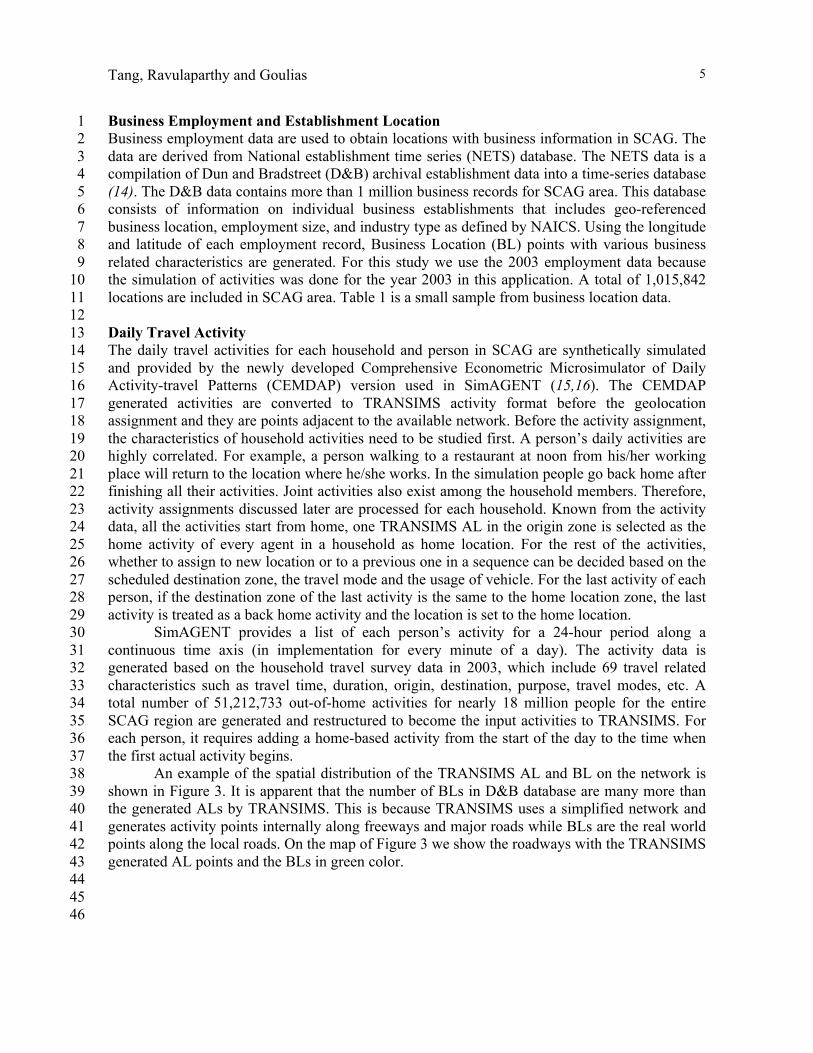
An example of the spatial distribution of the TRANSIMS AL and BL on the network is 38 shown in Figure 3. It is apparent that the number of BLs in D&B database are many more than 39 the generated ALs by TRANSIMS. This is because TRANSIMS uses a simplified network and 40 generates activity points internally along freeways and major roads while BLs are the real world 41 points along the local roads. On the map of Figure 3 we show the roadways with the TRANSIMS 42 generated AL points and the BLs in green color. 43 44 45 46


1 TABLE 1 Sample of Business Locations 2

3 4

5 FIGURE 1: Network of SCAG in TRANSIMS 6

ID ADDRESS X_COORD Y_COORD CITY STATE ZIPCODE ZIP4 LEVELCODE EMP03 EMPHERE SIC2 SIC3 SIC03 INDUSTRY

101546719 PALMERA -117.598 33.6343RANCHO SANTA MARGRTA CA 92688 1336 Z 1 1 72 721 72170000Carpet and upholstery cleaning

10154686363 WILSHIRE BLVD -118.367 34.0637LOS ANGELES CA 90048 5701 D 3 3 47 472 47240000 Travel agencies

10154695020 CAMPUS DR -117.857 33.668NEWPORT BEACH CA 92660 2120 D 2 2 50 506 50650000Electronic parts and equipment, nec

1015470119 SANDPIPER LN -117.744 33.5985ALISO VIEJO CA 92656 1805 D 2 2 7 78 7810200Landscape services

10154711194 E BRIER DR -117.261 34.0712SAN BERNARDINO CA 92408 2838 D 40 40 87 874 87420300Marketing consulting services

101547211755 WILSHIRE BLVD -118.462 34.0486LOS ANGELES CA 90025 1506 D 15 15 63 633 63310000Fire, marine, and casualty insurance

101547321219 FIGUEROA ST -118.286 33.8363 CARSON CA 90745 1941 D 45 6 48 484 48419901Cable television services

101547416500 VALLEY VIEW AVE -118.029 33.8817 LA MIRADA CA 90638 5822 D 15 10 50 502 50210200Household furniture

10154751230 MADERA RD 5-103 -118.796 34.2613SIMI VALLEY CA 93065 4045 D 4 4 87 874 87420300Marketing consulting services

10154769440 SANTA MONICA BLVD PH -118.403 34.0713BEVERLY HILLS CA 90210 4622 D 2 2 62 621 62110000Security brokers and dealers

10154778120 MELBA AVE -118.634 34.2172CANOGA PARK CA 91304 3532 D 2 2 87 874 87420300Marketing consulting services

10154781631 W 135TH ST -118.305 33.9093 GARDENA CA 90249 2505 D 5 23 51 514 51410000Groceries, general line

10154799600 IRONDALE AVE -118.586 34.2445CHATSWORTH CA 91311 5008 D 13 13 17 171 17110400Heating and air conditioning contractors

101548062028 MOUNTAIN VIEW CIR -116.31 34.1305JOSHUA TREE CA 92252 2523 D 14 14 52 521 52110303Solar heating equipment


1 FIGURE 2 Examples of time of day availability for different business types 2


1 FIGURE 3 An example of SimAGENT-TRANSIMS activity locations (red dots) and real 2 world business locations (green dots) 3 4 METHODOLOGY 5 To match the daily SimAGENT activities with businesses in both space and time we follow the 6 flowchart of Figure 4. With the destination TAZ and the purpose of every activity from 7 SimAGENT, a collection of ALs within the TAZ and the BLs by business type matching to the 8 activity purpose are both selected. Then, employee availability is used to match workers to 9 locations by industry type as explained below. 10

Consider a zone i within the SCAG region (the region contains 4192 zones, 11 i=1,2,...,4192). The total number of available locations in zone i at time period T is !! ! . The 12 universe of all available locations at time T for the entire SCAG region is: 13

14 !(!) = ! !! ! !!"#$

!!! (1) 15 16 To reflect the time of day change in availability of activity opportunities we compute the 17

number of available locations in zone i in period T. In equations, the number of available BLs in 18 zone i at period T is: 19 20

!!(!) = ! ! !!"# ,!!"#(!)!!!!! ! !!"# ,!!"#(!) = 1, !!"#×!!"#(!) ≥ 1

0, !!"#×!!"#(!) < 1 ! ! ! ! (2)!21

22 Where, !! – number of business locations in zone ! 23 !!"# – employment size of the business location j in zone i with the activity type of k 24 !!"# ! – percentage of available workers of business location j in zone i with business type of k 25 by the function of time T 26 ! !!"# ,!!"#(!) – indicator function of !!"# and !!"#(!) 27


In this study, a county wide percentage of available workers by time of day T is applied 1 to each individual business location j which belong to zone i for business type k. Let’s take zone 2 “584” as an example. The total number of available business locations is 405. These 405 3 business locations are connected to its nearest AL and categorized in 15 different industry types. 4 The business type of BL “135293” in Zone “584” is “Construction” in Los Angeles County. And 5 its employment size is “17” which is !!"# in equation (2). We can then search the business 6 accessibility matrices of LA county to find the correspondent percentages of “Construction” for a 7 whole day. For example, at 10:00 AM, the percentage is 52.03% while at 5:00 PM it is 11.53%. 8 And the available workers can be calculated in location “135279”. The available workers are 8 9 (17*52.03%) at 10:00 and 1 (17*11.53%) at 17:00 which are used to compute !!"#×!!"#(!) in 10 equation (2). With this calculation, the available workers for the entire time of day can be 11 obtained. When it comes to the activity assignment, from the ActivityType_IndustrialType cross 12 matrices, the activity can be assigned to the AL which connected to the BL “135293” with an 13 activity type of “work”. However, more than one business locations belong to work activity. 14 Therefore, only one location can be selected and assigned to the activity record from all the 15 available BLs that correspond to the same activity ALs. 16

Closeness between ALs and BLs is decided according to the geographic coordinates of 17 both locations, Euclidean distances are calculated for each BL to every ALs. Based on the 18 distances, the AL with the shortest distance is selected as the correspondent location to BL. The 19 BL and the selected AL are defined as a location pair. After that, a new location file that has both 20 attributes from BL and AL is created from the pair. When activity is assigned to one business 21 location, the specified AL in TRANSIMS can be located through the new location data. From 22 Figure 5, the allocation of BLs to ALs is shown by the arrows. 23

The BL-AL connection approach mathematically is presented below. Let us define A is 24 the set of TRANSIMS activity locations. B is the set of business locations; The !!! in set !′ is 25 the objective location where Euclidean distance !(!!,!!) is the shortest !!"# in the distance 26 set !!. !!!,!!!!,!!!,!!!are the latitude and longitude coordinates of !! and !!. The formulas 27 are as follows: 28 29 !! = !!! ,!!! ,⋯!!! (3) 30 !!! = !!!!!!"# !!"# ∈ !! (4) 31 !! = ! !!,!! ,! !!,!! ⋯! !!,!! |! ∈ !,! ∈ ! (5) 32

!(!!,!!) = (!!! − !!!)! + (!!! − !!!)! (6) 33

34 The BL-based geolocation assignment for activities is implemented in 35

SimAGENT-TRANSIMS activity conversion. The first location of each person is treated as the 36 home location, which is randomly chosen from the origin zone. The other locations where the 37 actual activity happens are selected based on the proposed assignment approach. Figure 6 shows 38 a distribution of the activity locations used in geolocation assignment in downtown Los Angeles 39 area. Different colors of the points in the figure indicate different range of the times that have 40 been geolocated. The red locations are assigned to more activities compared with the blue ones. 41 The difference in the number of location distribution in each zone illustrates that the activity 42 assignment is directional. 43

After location assignment for each person, activities are input to TRANSIMS for travel 44 demand modeling. The daily activities are input into TRANSIMS router to generate the travel 45


plans. For the entire SCAG area, the travel plans that are generated for all the residents have 1 65,848,153 activity records and 1,360,348 goods movement trips in total. A parallelization 2 scheme is carried out for travel demand modeling. The computation is done on a workstation 3 with 12 CPU cores at 3.2GHZ and takes about 23 hours for the routing process. The plan and 4 link summarize programs in TRANSIMS are used to compute the traffic volumes and speed on 5 each network link. The typical TRANSIMS model follows in Figure 7. 6

The travel demand modeling for activity with BL-based assignment is conducted in 7 TRANSIMS. It is an integrated system of travel forecasting models designed to give 8 transportation planners more accurate and complete information on traffic impacts, congestion, 9 and pollution. The travel demand model in TRANSIMS is an iterative process. The model flow 10 is shown in Figure 7. The router reads individual activities and creates a series of travel paths 11 called travel plans and they composed of travel mode, time period of travel, origin destination 12 locations and a minimum impedance travel path between the origin and destination locations. 13 Using Bureau of Public Roads (BPR) based traffic assignment function the software estimates 14 link delays. In the initial step, based on the number of trips through each link, the PlanSum 15 program summarizes all the travel plans. The LinkDelay program weights the new link delay 16 data with the previous one and generates a new weighted link delay file for the current iteration. 17 By comparing the travel plans and link delay, PlanSelect program creates a subset of households 18 to re-route on the network and determines the optimized route for each selected person while 19 creating new plans. The new plans will merge with the previous travel plans and start the next 20 iteration. The iterations will stop and traffic results are computed when the result comes to some 21 kind of User Equilibrium (UE). 22

The LinkSum program generates a variety of traffic related results�including link data 23 files of volumes, speeds, travel times, volume/capacity ratios, travel time ratios, delay, average 24 density, maximum density, average queue, maximum queue, and cycle failures summarized by 25 time of day, report the links with the top 100 link volumes, lane volumes, period volumes, speed 26 reductions, V/C ratios, travel time ratios, volume changes, or travel time changes and the link 27 groups with total volumes greater than user specified values, report the distribution of travel time, 28 V/C ratio, travel time change, and volume change by lane kilometer and time period. It can also 29 calculate congestion duration-based measures by aggregating time periods with time ratios 30 greater than a specified value and report various network performance statistics. In this paper, a 31 link-by-link volume and average speed files are generated and compared between two methods 32 of assigning activities to activity locations. 33


1 FIGURE 4 Assignment of activities with new business locations 2 3 4

5 FIGURE 5: Allocation of activity locations and business locations 6 7

Activity'RecordHousehold)IDPerson)IDActivity)TypeStart)TimeEnd)TimeDurationOriginDestination�

New'Business'LocationsIDX)CoordY)CoordSIC)CodeNAICS)CodeEmployee)by)TimeLocation)ID)in)TRANSIMSZone)ID�

Activity)Type

NAICS)Code

NAICSFActivity)TypeCross)Matrices

Origin)/)Destination)Zone

Employee)by)Time

Start)/)End)Time

Location)list)by)Zone

Available)Locations Assign)Activity)to)one)location


1 FIGURE 6: Distribution of activity assigned of locations in downtown Los Angeles 2 3

4 FIGURE 7: Travel demand model in TRANSIMS 5 6 7

Router

PlanSum

LinkDelay

PlanSelect

Re3Route

User6Equilibrium

NO

LinkSum

YES

Input6Data


IMPLEMENTATION 1 The assignment and traffic demand modeling are carried out in SCAG region. Travel activity 2 data generated from SimAGENT are used as input for travel demand modeling instead of 3 TRANSIMS self-generated activities. Apart from travel activity data for passengers, goods 4 movement trips from four-step-model are added for travel demand modeling as well. C# 5 programs were developed to achieve all the data conversions and the BL based activity 6 assignment. Due to the network limitation in TRANSIMS, when building the connections 7 between AL and BL, AL may be connected to more than one business location. Although some 8 ALs are connected with many BLs, it will not bring about major impacts on the current road 9 network in traffic demand modeling because the differences only impacts roadways between AL 10 to BL, which are excluded from TRANSIMS network. To better understand the geolocation 11 assignment influence on travel demand modeling, a comparative study between business location 12 based assignment and random activity location assignment is conducted for the 13 SimAGENT-TRANSIMS application as well. For random location assignment, all activity 14 locations are the same and treated equally. Locations are selected randomly from TRANSIMS 15 activity locations without considering the business characteristics and time availability, thus 16 leading to a relatively balanced assignment in each zone. 17

The link volumes and average speed per 15 minutes have been chosen for comparison 18 and are analyzed and computed using TRANSIMS link summarize program. Figure 8 shows the 19 comparison of volumes on one major local road, one freeway and the total network roadways 20 while the comparison of average speed is shown in Figure 9. From Figure 8, the total traffic 21 volume estimated for the entire study region for both the assignment models are not significantly 22 different and the two volumes are almost identical. Comparing the volume and speed on local 23 roadways and freeways, the differences of the two volumes on local road exist from morning 24 until midnight. While on freeway, the volumes remain almost the same before 15:00. After 15:00, 25 however, small differences emerge. As expected, the traffic volumes on local roads are affected 26 by the BL-based geolocation assignment. 27

A similar conclusion can be reached from the average speed comparison on three 28 different road types for two assignment methods. With the higher volume, the average speed is 29 lower. Differences in speeds on local roads are observed while computed speeds on freeways 30 remain almost the same. 31

In addition to the volume comparison in the charts, Figure 10 shows the numerical 32 differences of the two volumes on the map in four time periods. Combined with this map, the 33 BL-based assignment mainly makes impact on the local road rather than the freeways in traffic 34 demand modeling. In summary, first, the location assignment method allocates activities to 35 different locations only within the destination zone. The connection paths between origin and 36 destination zones, which are mostly on freeways, still remain the same. Second, from the chart in 37 Figure 9, the volume computed with BL-based geolocated activities is higher than the one with 38 randomly distributed activities from 17:00 to 23:00. This may be caused by the locations for BL 39 activity assignment is restricted by time, and most business locations are closed in the evening 40 according to business schedules. The activities are assigned to the limited locations which can 41 cause the difference due to spatial aggregation of trips and the average distance per trip is longer 42 at night than the trips during the day time. Therefore, local roads and trips in the evening are 43 influenced more by the BL assignment method. 44 45


FIGURE 8: Time of day volume comparison 1 2

0

5,000,000

10,000,000

15,000,000

20,000,000

0:15

1:

00

1:45

2:

30

3:15

4:

00

4:45

5:

30

6:15

7:

00

7:45

8:

30

9:15

10

:00

10:4

5 11

:30

12:1

5 13

:00

13:4

5 14

:30

15:1

5 16

:00

16:4

5 17

:30

18:1

5 19

:00

19:4

5 20

:30

21:1

5 22

:00

22:4

5 23

:30

Volu

me

Total Volume

Random Assignment BL-based Assignment

0

200

400

600

800

0:15

1:

00

1:45

2:

30

3:15

4:

00

4:45

5:

30

6:15

7:

00

7:45

8:

30

9:15

10

:00

10:4

5 11

:30

12:1

5 13

:00

13:4

5 14

:30

15:1

5 16

:00

16:4

5 17

:30

18:1

5 19

:00

19:4

5 20

:30

21:1

5 22

:00

22:4

5 23

:30

Volu

me

Volume on Local Road


0

1,000

2,000

3,000

4,000

0:15

1:

00

1:45

2:

30

3:15

4:

00

4:45

5:

30

6:15

7:

00

7:45

8:

30

9:15

10

:00

10:4

5 11

:30

12:1

5 13

:00

13:4

5 14

:30

15:1

5 16

:00

16:4

5 17

:30

18:1

5 19

:00

19:4

5 20

:30

21:1

5 22

:00

22:4

5 23

:30

Volu

me

Volume on Freeway



1

FIGURE 9: Time of day average speed comparison 2

20

25

30

35

40

45 0:

15

1:00

1:45

2:30

3:15

4:00

4:45

5:30

6:15

7:00

7:45

8:30

9:15

10:0

0

10:4

5

11:3

0

12:1

5

13:0

0

13:4

5

14:3

0

15:1

5

16:0

0

16:4

5

17:3

0

18:1

5

19:0

0

19:4

5

20:3

0

21:1

5

22:0

0

22:4

5

23:3

0

Mile

/Hou

r Total Average Speed

BL-based Assignment Random Assignment

20

25

30

35

40

45

0:15

1:

00

1:45

2:

30

3:15

4:

00

4:45

5:

30

6:15

7:

00

7:45

8:

30

9:15

10

:00

10:4

5 11

:30

12:1

5 13

:00

13:4

5 14

:30

15:1

5 16

:00

16:4

5 17

:30

18:1

5 19

:00

19:4

5 20

:30

21:1

5 22

:00

22:4

5 23

:30

Mile

/Hou

r

Average Speed on Local Road


0

20

40

60

80

0:15

1:00

1:45

2:30

3:15

4:00

4:45

5:30

6:15

7:00

7:45

8:30

9:15

10:0

0

10:4

5

11:3

0

12:1

5

13:0

0

13:4

5

14:3

0

15:1

5

16:0

0

16:4

5

17:3

0

18:1

5

19:0

0

19:4

5

20:3

0

21:1

5

22:0

0

22:4

5

23:3

0

Mile

/Hou

r

Average Speed on Freeway


Tang, Ravulaparthy and G

oulias

16

1

(a) Volum

e difference at 3:00 (b): Volum

e difference at 9:00 2

3

(c) Volum

e difference at 15:00 (d): Volum

e difference at 21:00 4

FIGU

RE

10 Volum

e differences between B

L-based and random

assignment

5


SUMMARY AND CONCLUSION 1 In this paper, a new approach is proposed for assigning daily travel activities onto a network 2 using real world business locations and time dependent activity assignment. Before the 3 assignment, real business locations are merged with time of day availability of the employees in 4 these businesses data that are connected to the corresponding activity location in TRANSIMS. 5 With the location pairs, the activities from SimAGENT (the activity based approach of SCAG) 6 are successfully assigned in a directional way. After that, activities serve as input for 7 activity-based travel demand modeling in TRANSIMS. Based on the link-by-link result of traffic 8 volumes and average speed, comparisons are carried out between BL-based geolocation 9 assignment and random assignment. The results from BL-method indicate significant differences 10 in traffic volume estimation on local roads when compared with random assignment procedure. 11 This variation in traffic demand estimation between the two methods needs to be further 12 validated with existing traffic counts on a link-by-link basis to reach definitive conclusions about 13 the performance of the BL-based geolocation assignment procedure. In parallel, a home 14 geolocation assignment is currently developed to complete the method presented in this paper. 15 Moreover, the possibility of business establishments serving different types of activities duirng a 16 day is also currently examined and may lead us to modify the method presented in this paper 17 (17). Thus, a time-based point-to-point geolocation method for activity assignment can be 18 addressed. Such assignment could bring about many benefits. First, geolocating activities to real 19 business location provides more detailed individual travel route with personal travel purpose 20 considered, thus aiding in developing a finer resolution travel demand model. Second, the 21 detailed route could, in turn, contribute to better analysis of emissions, GHGs and its influence 22 on the environment. Third, the traffic demand modeling and impacts analysis of small areas are 23 both strengthened and enhanced. Fourth, the different times business location is used as 24 destination in different time period could give out another way for the regional traffic impact 25 analysis. From another perspective, since it is local roads that are most impacted by the spatial 26 assignment, in future studies we will need to examine more carefully local roads and develop 27 methods that assign activities along local roads. 28 29 ACKNOWLEDGMENTS 30 Funding for this research is provided by the Southern California Association of Governments, 31 The University of California Transportation Center, and the University of California Office of 32 the President for the Multi-campus Research Program Initiative on Sustainable Transportation 33 and the UC Lab Fees program on Next Generation Agent-based Simulation. This paper does not 34 constitute a policy or regulation of any Local, State, or Federal agency. 35


REFERENCES 1 2 1. Bradley, M., J. L. Bowman and B. Griesenbeck. (2010). SACSIM: An applied activity-based 3

model system with fine-level spatial and temporal resolution, Journal of Choice Modeling, 4 Vol, 3(1), 2010. 5

2. Hao, J.Y., (2010). TASHA-MATSim Integration and its Application in Emission Modelling. 6 Master Thesis, University of Toronto, Canada. 7

3. Bradley, M., Bowman, J. L., Shiftan, Y., Lawton, T. K. and Ben-Akiva, M. E., (1998). A 8 System of Activity-Based Models for Portland, Oregon. Report prepared for the Federal 9 Highway Administration Travel Model Improvement Program. Washington, D.C. 10

4. Bradley, M., Outwater, M., Jonnalagadda, N., and Ruiter, E. (2001). Estimation of an 11 Activity-Based Micro-Simulation Model for San Francisco, Paper presented at the 80th 12 Annual meeting of the Transportation Research Board, Washington D.C., 2001. 13

5. Vovsha P., Petersen, E. and Donnelly, R. (2002). Micro-Simulation in Travel Demand 14 Modeling: Lessons Learned from the New York Best Practice Model. Transportation 15 Research Record 1805, 68-77, 2002. 16

6. Bowman, J. L., Bradley, M. and Gibb, J. (2006). The Sacramento Activity-based Travel 17 Demand Model: Estimation and Validation Results. Paper presented at the European 18 Transport Conference, Strasbourg, France, September 18-20. 19

7. Beckman, R. J. (1997). TRANSIMS Dallas/Fort Worth case study report. Los Alamos 20 Unclassified Report (LA-UR), Los Alamos National Laboratory, TSA-Division, Los Alamos, 21 NM, 87545. 22

8. Rilett, L. R. (2001). Transportation planning and TRANSIMS microsimulation model: 23 Preparing for the transition. Transportation Research Record: Journal of the Transportation 24 Research Board, No.1777, 84-92, 2001. 25

9. Gao, W., Balmer, M., Miller, E. J. (2010). Comparison of MATSim and EMME/2 on greater 26 Toronto and Hamilton area network, Canada.Transportation Research Record: Journal of the 27 Transportation Research Board, No.2197, 118-128, 2010. 28

10. Balmer, M., Rieser, M. (2004). Generating daily activity chains from origin-destination 29 matrices. Transportation Research Board 84th Annual Meeting, 2004. 30

11. Goulias, K.G., C. R. Bhat, R. M. Pendyala, Y. Chen, R. Paleti, K. Konduri, S. Y. Yoon, and 31 D. Tang. (2012). SimAGENT Overview. Phase 2 Final Report 1 Submitted to SCAG, March 32 31, 2012, Santa Barbara, CA. 33

12. Goulias, K.G., C.R. Bhat, R.M. Pendyala, Y. Chen, R. Paleti, K.C. Konduri, T. Lei, D. Tang, 34 S.Y. Yoon, G. Huang, H.H. Hu. (2011). Simulator of activities, greenhouse emissions, 35 networks, and travel (SimAGENT) in Southern California, Paper submitted for presentation 36 at the 91st Annual Meeting of the Transportation Research Board, Washington, D.C. 37

13. Chen, Y., S. Ravulaparthy, K. Deutsch, P. Dalal, S.Y. Yoon, T. Lei, K.G. Goulias, R.M. 38 Pendyala, C.R. Bhat, and H-H. Hu. (2011). Development of Opportunity-based Accessibility 39 Indicators, Paper presented at the 90th 20 Annual Transportation Research Board Meeting, 40 Washington D.C., January 23-21 27, 2011 and Transportation Research Record. 41

14. Walls, D. (2007). National Establishment Time Series Database: Data Overview, 2007 42 Kauffman Symposium on Entrepreneurship and Innovation Data. 43

15. Bhat, C.R., Guo, J.Y., Srinivasan, S. and Sivakumar, A. (2004). A Comprehensive 44 Econometric Microsimulator for Daily Activity-Travel Patterns, Transportation Research 45 Record, Vol. 1894, pp. 57-66, 2004. 46


16. Bhat C. R., K.G. Goulias, R.M. Pendyala, R. Paleti, R. Sidhartan, L. Schmitt, and H. Hu 1 (2012). A Household-Level Activity Pattern Generation Model: Simulator of Activities, 2 Greenhouse Emissions, Networks, and Travel (SimAGENT) System in Southern California, 3 Paper 12-4226 presented at the 91st Annual Meeting of the Transportation Research Board, 4 Washington, D.C. 5

17. Yoon, S.Y., Ravulaparthy, S. and Goulias, K.G. (2012). Dynamic diurnal social taxonomy of 6 urban environments. 13th International Conference on Travel Behavior Research, Toronto, 7 July 15-20, 2012. 8

1 geolocating activities to business establishment ... · tang, ravulaparthy and goulias 1 1...

Documents