1

Geometric TransformationGeometric TransformationGeometric TransformationGeometric Transformation

Operations depend on pixel’s Coordinates.

Context free.

Independent of pixel values.

',

',

yyxfy

xyxfx

y

x

yxfyxfIyxI yx ,,,'),(

(x’,y’)(x,y)

I(x,y) I’(x’,y’)

• Example: Translation

1,

3,

yyxfy

xyxfx

y

x

),(1,3' yxIyxI

(x,y)

I(x,y) I’(x’,y’)

(x’,y’)

Forward MappingForward MappingForward MappingForward Mapping

Forward mapping:

Forward Mapping

Source Target

yyxfy

xyxfx

y

x

,

,

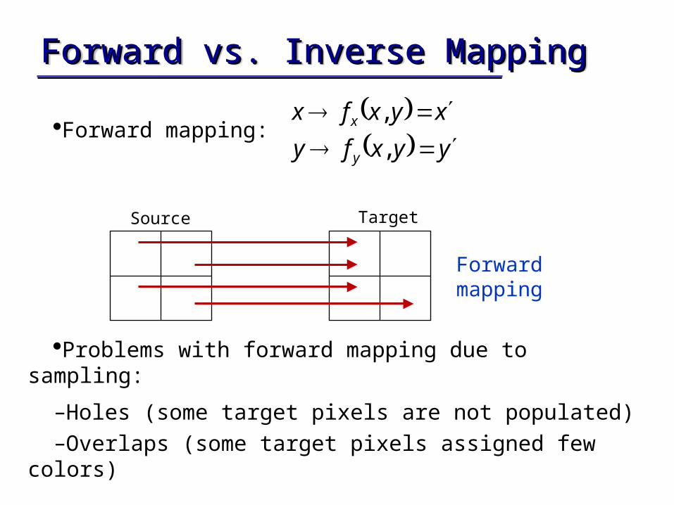
Forward vs. Inverse MappingForward vs. Inverse MappingForward vs. Inverse MappingForward vs. Inverse Mapping

Forward mapping:

Problems with forward mapping due to sampling:

–Holes (some target pixels are not populated)–Overlaps (some target pixels assigned few colors)

Forward mapping

Source Target

yyxfy

xyxfx

y

x

,

,

Inverse mapping:

Each target pixel assigned a single color.

Color Interpolation is required.

InverseMapping

yyxfy

xyxfx

y

x

,

,1

1

TargetSource

• Example: Scaling along X

– Forward mapping:

– Inverse mapping:

(0,0)(0,0)

Source Target

Source Target

yyxx ;2

yyxx ;2/

InterpolationInterpolationInterpolationInterpolation

• What happens when a mapping function calculates a fractional pixel address?

• Interpolation: generates a new pixel by analyzing the surrounding pixels.

• Good interpolation techniques attempt to find an optimal balance between three undesirable artifacts: edge halos, blurring and aliasing.

9

InterpolationInterpolationInterpolationInterpolation

x4 scaling

N.N Bilinear Bicubic

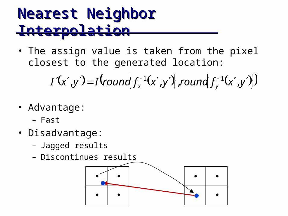
Nearest Neighbor InterpolationNearest Neighbor InterpolationNearest Neighbor InterpolationNearest Neighbor Interpolation

• The assign value is taken from the pixel closest to the generated location:

• Advantage: – Fast

• Disadvantage: – Jagged results– Discontinues results

yxfroundyxfroundIyxI yx ,,,, 11

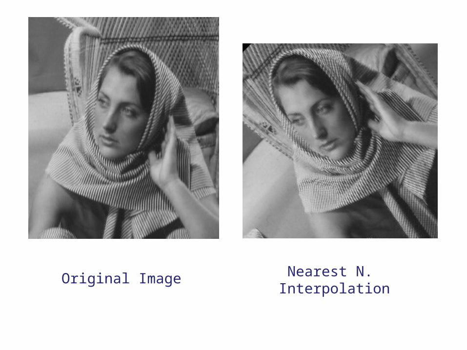
Original Image Nearest N. Interpolation

Original Image

Nearest N. Interpolation

Bilinear InterpolationBilinear InterpolationBilinear InterpolationBilinear Interpolation

• The assigned value is an intermediate value between the four nearest pixels:

Linear InterpolationLinear InterpolationLinear InterpolationLinear Interpolation

• Isolating v in the above equation:

xw xe

vw

ve

x

v

we

w

we

w

vv

vv

xx

xx

we vvv 1we

w

xx

xxwhere

Bilinear InterpolationBilinear InterpolationBilinear InterpolationBilinear Interpolation

• The assign value is a weighted sum of the four nearest pixels.

• Each weight is proportional to the distance from each existing pixel.

NWNE

SESW

s

tS

NV

• The bilinear interpolation is the best fit low-degree polynomial of the form:

• The pixel’s boundaries are C0 continuous (continuous values across boundaries).

ji

jiij tsatsv

1

0,

),(

sNEsNWNsSEsSWS 1;1

tNtSV 1

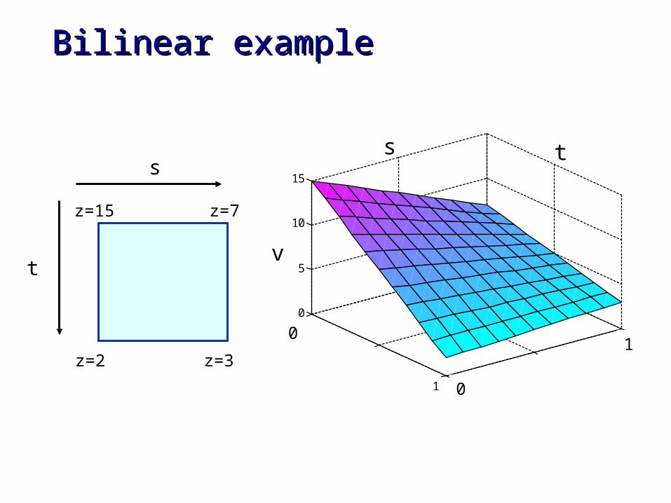
Bilinear exampleBilinear example

z=15 z=7

z=2 z=3

s

t

1

1.5

2

1

1.5

20

5

10

15

v

s t

0

10

Nearest N.Interpolation

Bilinear Interpolation

Nearest N.Interpolation

Bilinear Interpolation

Bicubic InterpolationBicubic InterpolationBicubic InterpolationBicubic Interpolation

• The assign value is a weighted sum of the 4x4 nearest pixels:

ji

jiij tsatsv

3

0,

),(

How can we find the right coefficients?

• Denote the pixel values Vpq {p,q=0..3}

• The unknown coefficients are aij {i,j=0..3}

21

]2,1[,},3..0{,3

0,

tsqpfortsav ji

jiijpq

s

t

• We have a linear system of 16 equations with 16 coefficients.

• The pixel’s boundaries are C1 continuous (continuous derivatives across boundaries).

N.N Bilinear Bicubic

N.N

Bilinear

Bicubic

Applying the TransformationApplying the TransformationApplying the TransformationApplying the Transformation

T = …… % 2x2 transformation matrix[r,c] = size(img)

% create array of destination x,y coordinates[X,Y]=meshgrid(1:c,1:r);

% calculate source coordinatessourceCoor = inv(T) * [X(:) Y(:) ] ‘ ;

% calculate nearest neighbor interpolation Xs = round(sourceCoor(1,:));Ys = round(sourceCoor(2,:));

indx=find(Xs<1 | Xs>r); %out of range pixelsXs(indx)=1; Ys(indx)=1;

indy=find(Ys<1 | Ys>c); %out of range pixelsXs(indy)=1; Ys(indy)=1;

% calculate new imagenewImage = img((Xs-1).*r+Ys);newImage(indx)=0; newImage(indx)=0; newImage = reshape(newImage,r,c);

Types of linear 2D transformationsTypes of linear 2D transformationsTypes of linear 2D transformationsTypes of linear 2D transformations

• Rigid (Euclidean) transformation:– Translation + Rotation (distance preserving).

• Similarity transformation:– Translation + Rotation + Uniform Scale (angle preserving).

• Affine transformation:– Translation + Rotation + Scale + Shear (parallelism preserving).

• Projective transformation – Cross-ratio preserving

• All above transformations are groups where Rigid

Similarity Affine Projective

Homogeneous CoordinatesHomogeneous CoordinatesHomogeneous CoordinatesHomogeneous Coordinates

• Homogeneous Coordinates is a mapping from Rn to Rn+1:

• Note: (tx,ty,t) all correspond to the same non-homogeneous point (x,y). E.g. (2,3,1)(6,9,3) (4,6,2).

• Inverse mapping:

yx,,,,

W

Y

W

XWYX

),,(),,(),( ttytxWYXyx

Some 2D TransformationsSome 2D TransformationsSome 2D TransformationsSome 2D Transformations

• Translation :

• Affine transformation:

• Projective transformation:

11100

10

01

y

x

y

x

ty

tx

y

x

t

t

W

Y

X

1100

y

x

tdc

tba

W

Y

X

y

x

11

y

x

fe

tdc

tba

W

Y

X

y

x

Hierarchy of Linear 2D TransformationsHierarchy of Linear 2D TransformationsHierarchy of Linear 2D TransformationsHierarchy of Linear 2D Transformations

Non Linear 2D TransformationsNon Linear 2D TransformationsNon Linear 2D TransformationsNon Linear 2D Transformations

• Non linear transformations do not necessarily preserve straight lines.

• Methods:– Piecewise linear transformations– Non linear parametric mapping

• Non linear mapping:

• Example: non linear (radial) lens distortions:

ji

jiij tsatsx

,

,

ji

jiij tsbtsy

,

,

Transformation EstimationTransformation EstimationTransformation EstimationTransformation Estimation

• Let: x’=fx(x,y,px) ; y’=fy(x,y,py), where px and py are vector of parameters.

• If the mappings are linear in px and py the parameters can be estimated using linear regression.

• Example: Affine transformation

• Alternative representation:

1100

y

x

tdc

tba

W

Y

X

y

x

y

x

t

t

d

c

b

a

yx

yx

y

x

1000

0100

• Given k points (P1,P2,..Pk) in 2D that have been transformed to (P'1,P'2,..,P'k) by affine transformation:

– How many points uniquely define the affine (projective) transformation?

– How can we find the affine transformation?

– What if we have more points?

– What can be done if points coordinates are inaccurate?

bMMMp

bMpp

bMp

TT

a

1ˆ

minˆ

Image Warping and MorphingImage Warping and MorphingImage Warping and MorphingImage Warping and Morphing

• Image rectification.

• Key frame animation.

• Image Synthesis

– Facial expression

– Viewing positions

Image Metamorphosis.

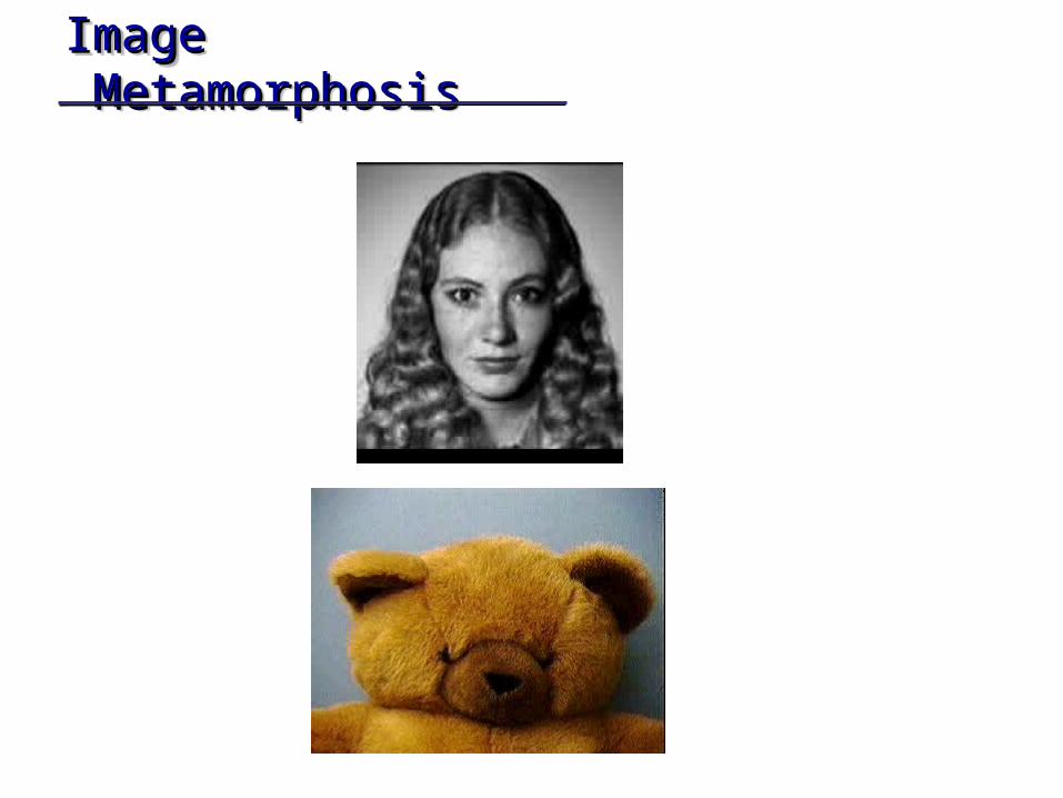
Image MetamorphosisImage Metamorphosis Image MetamorphosisImage Metamorphosis

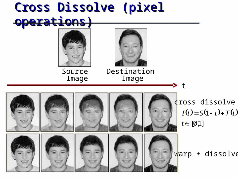
Cross Dissolve (pixel operations)Cross Dissolve (pixel operations)Cross Dissolve (pixel operations)Cross Dissolve (pixel operations)

Destination Image

Source Image

]1,0[

1

t

tTtStI

t

cross dissolve

warp + dissolve

Warping + Cross DissolveWarping + Cross Dissolve Warping + Cross DissolveWarping + Cross Dissolve • Warp source image towards intermediate image.

• Warp destination image towards intermediate image.

• Cross-dissolve the two images by taking the weighted average at each pixel.

time

Cro

ss-d

isso

lve

warping images

source

destination

warp

warp

Cross-dissolve

Cross-dissolve

Image MetamorphosisImage MetamorphosisImage MetamorphosisImage Metamorphosis

• Let S,T be the source and the target images

• Let G(p) be the transformation from S towards T, where

G(0)=I the identity transformation

• Let t[0,1] the time step to be synthesized

Algorithm:

1. Warp S towards T:

2. Warp T toward S:

3. Cross dissolve:

StpGtS

TptGtT 11

tTttSttI 1

t

sourse

target

S(t)=G(tp){S}

T(t)=G((1-t)p)-1{T}

I(t)=(1-t)S(t)+t(T(t))

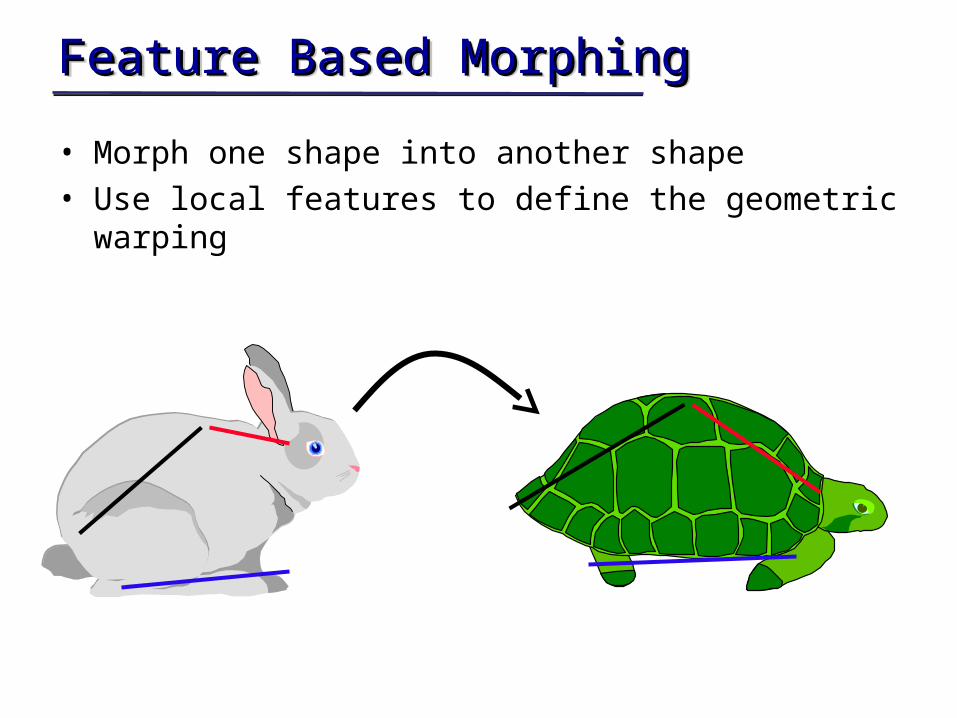
Feature Based MorphingFeature Based MorphingFeature Based MorphingFeature Based Morphing

• Morph one shape into another shape• Use local features to define the geometric warping

P

Q

P’

Q’

P

Q

P’

Q’

P

Q

P’

Q’

P

Q

P’

Q’

P

Q

P’

Q’

P

Q

P’

Q’

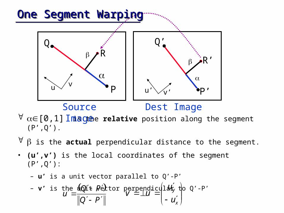
[0,1] is the relative position along the segment (P’,Q’).

is the actual perpendicular distance to the segment.

• (u’,v’) is the local coordinates of the segment (P’,Q’):

– u’ is a unit vector parallel to Q’-P’

– v’ is the unit vector perpendicular to Q’-P’

P

QR

P’

Q’

R’

Source Image Dest Image

u vu’ v’

PQ

PQu

x

y

u

uuv

One Segment WarpingOne Segment WarpingOne Segment WarpingOne Segment Warping

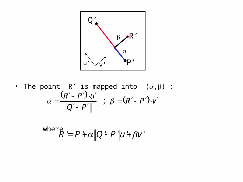
P’

Q’

R’

u’ v’

vPRPQ

uPR

;

• The point R’ is mapped into (,) :

where

'''''' vuPQPR

P

QR

P’

Q’

R’

Source Image Dest Image

u vu’ v’

Inverse Mapping:

where (u,v) is the local coordinates of the segment (P,Q):

vuPQPR ),(

PQ

PQu

x

y

u

uuv

Multiple Segment WarpingMultiple Segment WarpingMultiple Segment WarpingMultiple Segment Warping

• In multiple segment warping the point R’ is influenced by multiple segments.

• The influence strength of each segments is proportional to:– Segment length– The distance from the point R’

P1

Q1R1

1

P2

Q2 2

P1’

Q1’

R’’1

’2

P2’

Q2’

R2

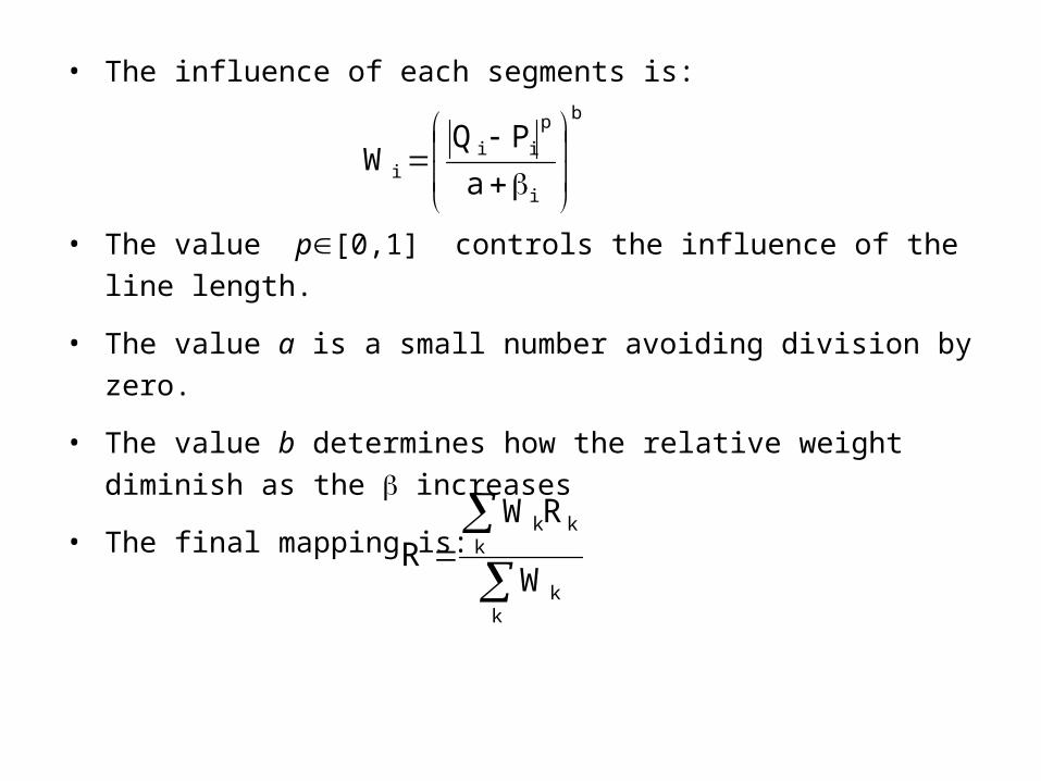
• The influence of each segments is:

• The value p[0,1] controls the influence of the line length.

• The value a is a small number avoiding division by zero.

• The value b determines how the relative weight diminish as the

increases

• The final mapping is:

b

i

p

iii a

PQW

kk

kkk

W

RWR

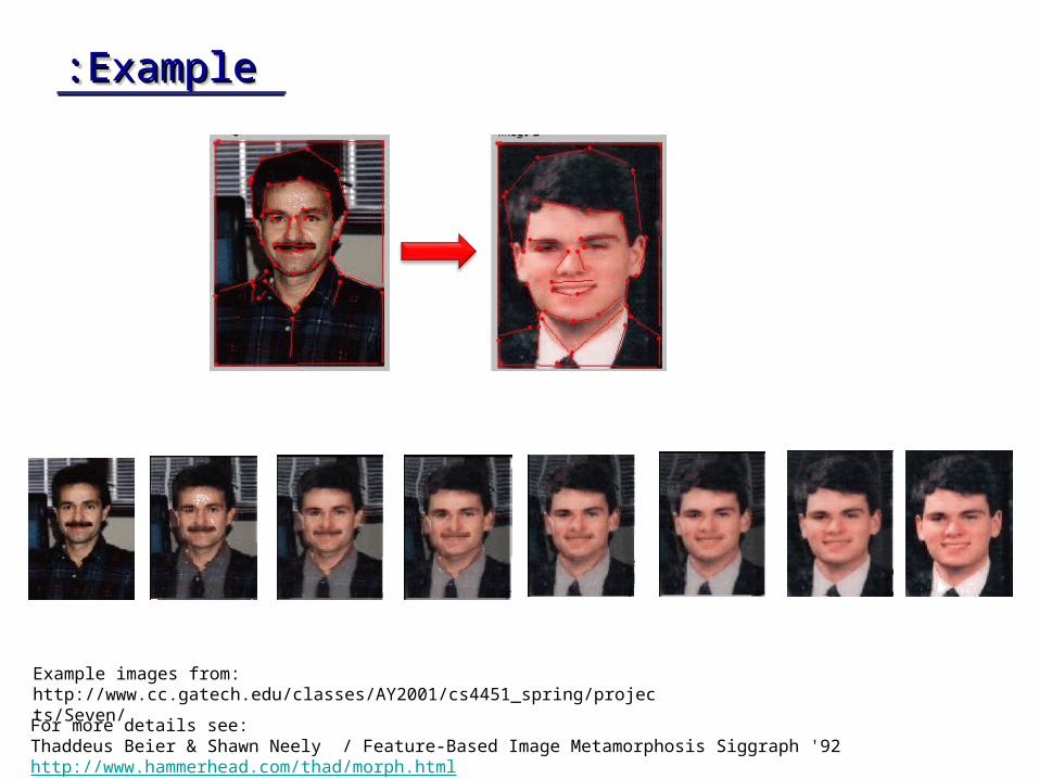
ExampleExample::ExampleExample::

For more details see:Thaddeus Beier & Shawn Neely  / Feature-Based Image Metamorphosis Siggraph '92 http://www.hammerhead.com/thad/morph.html

Example images from: http://www.cc.gatech.edu/classes/AY2001/cs4451_spring/projects/Seven/

56

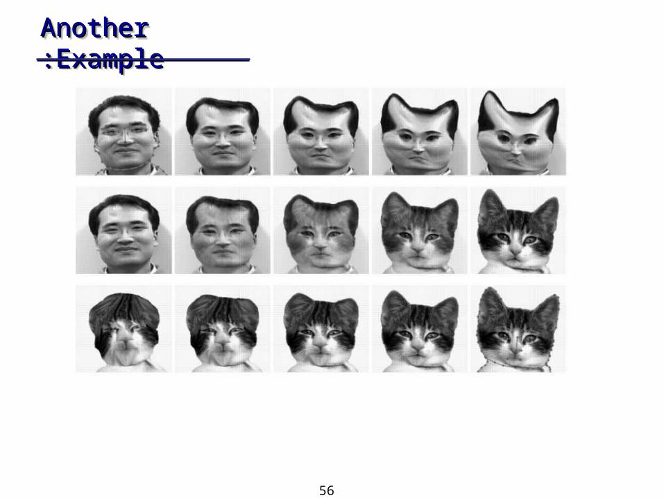
Another ExampleAnother Example::Another ExampleAnother Example::

T H E E N DT H E E N DT H E E N DT H E E N D